The Green’s function of the parabolic Anderson model and the continuum directed polymer

Abstract.

We build a regular version of the field $Z_{\beta}(t,x\hskip 0.7pt|\hskip 0.7pts,y)$ which describes the Green’s function, or fundamental solution, of the parabolic Anderson model (PAM) with white noise forcing on $\operatorname{\mathbb{R}}^{1+1}$: $\partial_{t}Z_{\beta}(t,x\hskip 0.7pt|\hskip 0.7pts,y)=$ $\frac{1}{2}\partial_{xx}Z_{\beta}(t,x\hskip 0.7pt|\hskip 0.7pts,y)+\beta Z_{\beta}(t,x\hskip 0.7pt|\hskip 0.7pts,y)W(t,x)$, $Z_{\beta}(s,x\hskip 0.7pt|\hskip 0.7pts,y)=\delta(x-y)$ for all $-\infty<s\leq t<\infty$, all $x,y\in\operatorname{\mathbb{R}}$, and all $\beta\in\operatorname{\mathbb{R}}$ simultaneously. Through the superposition principle, this gives a jointly continuous coupling of all solutions to the PAM with initial or terminal conditions satisfying sharp growth assumptions, for all initial and terminal times. We show that the PAM with a (sub-)exponentially growing initial condition has conserved quantities given by the limits $\displaystyle\lim_{x\to\pm\infty}x^{-1}\log Z_{\beta}(t,x)$, in addition to other new properties of solutions with general initial conditions. These are then connected to Hopf-Cole solutions to the KPZ equation and the existence, regularity, and continuity of the quenched continuum polymer measures. Through the polymer connection, we also show that the kernel $(x,y)\mapsto Z_{\beta}(t,x\hskip 0.7pt|\hskip 0.7pts,y)$ is strictly totally positive for all $t>s$ and $\beta\in\operatorname{\mathbb{R}}$.

1. Introduction

We study a regular realization of the five parameter field $Z_{\beta}(t,x\hskip 0.7pt|\hskip 0.7pts,y)$ which, for all $(s,y,t,x)\in\overline{\operatorname{\mathbb{R}}}_{{\scaleobj{0.8}{\uparrow}}}^{4}=\{(s,y,t,x)\in\operatorname{\mathbb{R}}^{4}:s\leq t\}$ and $\beta\in\mathbb{R}$, solves the family of stochastic partial differential equations

(1.1) $$\partial_{t}Z_{\beta}(t,x\hskip 0.7pt|\hskip 0.7pts,y) =\frac{1}{2}\partial_{xx}Z_{\beta}(t,x\hskip 0.7pt|\hskip 0.7pts,y)+\beta Z_{\beta}(t,x\hskip 0.7pt|\hskip 0.7pts,y)W(t,x)$$

$$Z_{\beta}(s,x\hskip 0.7pt|\hskip 0.7pts,y) =\delta(x-y),$$

where $W$ is space-time white noise and $\delta$ is the Dirac delta measure at $0$. This model is known variously as the parabolic Anderson model (PAM), as introduced in [10], or as the (linear) stochastic heat equation with multiplicative space-time white noise forcing. For linear equations like this one, such a process is commonly known as the Green’s function, or fundamental solution, of the equation. Our construction extends a previous construction of the Green’s function for this model in [1, 2] in a sense we elaborate on momentarily.

By the superposition principle, the construction of a field of solutions to (1.1) gives us a coupling of solutions to the PAM,

(1.2) $$\partial_{t}Z_{\beta}(t,x\hskip 0.7pt|\hskip 0.7pts;\mu) =\frac{1}{2}\partial_{xx}Z_{\beta}(t,x\hskip 0.7pt|\hskip 0.7pts;\mu)+\beta Z_{\beta}(t,x\hskip 0.7pt|\hskip 0.7pts;\mu)W(t,x)$$

$$Z_{\beta}(s,\cdot|s;\mu) =\mu(\cdot),$$

where $\mu$ is a positive Borel measure, for all initial times $s<t$ and inverse temperatures $\beta$ simultaneously through the identity

(1.3) $$Z_{\beta}(t,x\hskip 0.7pt|\hskip 0.7pts;\mu) =\int_{-\infty}^{\infty}Z_{\beta}(t,x\hskip 0.7pt|\hskip 0.7pts,y)\mu(dy).$$

When $\mu(dx)=f(x)dx$ for a sufficiently regular Borel measurable function $f$, which corresponds to function-valued initial conditions, we will instead write $Z_{\beta}(t,x\hskip 0.7pt|\hskip 0.7pts;f)$ as shorthand.

We take (1.3) as the definition of a physical solution to (1.2). This terminology is justified by analogy with the ordinary heat equation and by our results, which show that this definition is the unique jointly continuous process (as a function of all arguments including the measure or function valued initial condition) which agrees up to indistinguishability with the physically relevant mild formulation of (1.2) for fixed initial conditions. Note that even for the unforced heat equation with zero initial condition, there are non-physical classical solutions which are not given by the superposition principle [37, p. 184]. It is natural to expect similar non-physical weak solutions to exist here as well.

Using this construction, the main contributions of this work can be summarized as follows:

1. We produce a coupling of all solutions to (1.2) with general positive measure valued initial conditions, prove that these processes satisfy their initial conditions in senses stronger than those appearing previously in the literature, and verify that our coupling agrees with the usual mild formulation up to indistinguishability under the minimal measurability and moment conditions which have previously appeared in the literature.

2. We show that the coupling defined through (1.3), viewed as a process taking values in an appropriate Polish space of continuous functions (of $x$), is jointly continuous in the inverse temperature, the initial and terminal times, and the initial condition $\mu$, within the class of non-explosive initial conditions. This extends to a jointly continuous coupling of Hopf-Cole solutions to the KPZ equation ((1.9) below) started from the (sharp) class of non-explosive continuous initial conditions. By separability of the space of non-explosive initial conditions, such a coupling is necessarily unique up to indistinguishability. In particular, a corollary implies that the Hopf-Cole solution to the KPZ equation defines a Feller process on the space of non-explosive initial conditions.

3. We prove new uniform growth and path regularity estimates for solutions to (1.1), which imply new uniform growth and regularity estimates for solutions to (1.2). These estimates play a key role in essentially all of the proofs in this paper and are likely of independent interest.

4. Using our coupling and growth estimates, we prove a conservation law simultaneously for all times $s<t$ and all inverse temperatures $\beta$. Specifically, we show that if there exist $\lambda_{+},\lambda_{-}\in\operatorname{\mathbb{R}}$ such that

   $$\lim_{x\to\infty}\frac{\log f(x)}{x}=\lambda_{\pm},\qquad\text{ then }\qquad\lim_{x\to\pm\infty}\frac{\log Z_{\beta}(t,x\hskip 0.7pt|\hskip 0.7pts;f)}{x}=\lambda_{\pm}$$

   for all $s<t$ and $\beta\in\operatorname{\mathbb{R}}$. This generalizes the classical conservation law satisfied by the $\beta=0$ case of the ordinary heat equation.

5. We construct a simultaneous coupling of the continuum directed polymer measures for all initial and terminal conditions and all inverse temperatures, as well as proving many basic properties including weak and total variation regularity in the initial and terminal conditions, variants of the Feller and strong Feller properties, simultaneous Hölder $1/2-$ path regularity, and stochastic monotonicity as the initial condition varies. Essentially all of these properties are new.

6. Through analysis of the polymer measures and an argument based on the Karlin-McGregor theorem, we prove that the map $(x,y)\mapsto Z_{\beta}(t,x\hskip 0.7pt|\hskip 0.7pts,y)$ is strictly totally positive for all $t>s$ and $\beta\in\operatorname{\mathbb{R}}$. Essentially the same strict total positivity appears in [41] using a different argument.

We finally note that the results mentioned above provide the setting for a companion paper by the last three authors, [35], where synchronization, a quenched one force – one solution principle, and a characterization of ergodic stationary (modulo constants) distributions for the KPZ equation are proven.

Variants of the superposition principle for (1.2) have been observed previously in [1] and [16, Lemma 1.18] in particular, though without including the details which would determine precisely how generally solutions to (1.2) can be given by (1.3) and how generally these solutions can be coupled together. We show that the class of non-zero positive initial conditions for which (1.3) defines a solution to (1.2) for all $s<t$ and all $\beta\in\operatorname{\mathbb{R}}$ simultaneously is given by

(1.4) $$\operatorname{\mathcal{M}}_{{\scriptscriptstyle\textrm{HE}}} =\bigg{\{}\text{non-zero positive Borel measures }\mu\text{ on }\operatorname{\mathbb{R}}:\forall a>0,\int_{\operatorname{\mathbb{R}}}e^{-ax^{2}}\mu(dx)<\infty\bigg{\}}$$

and that all such solutions can be coupled simultaneously through the field in (1.1).

This condition matches the condition needed to define global solutions via the superposition principle for the case of $\beta=0$, i.e., the unforced heat equation. It also matches the conditions for existence of solutions to (1.2) for fixed $s\in\operatorname{\mathbb{R}}$, fixed $\mu\in\operatorname{\mathcal{M}}_{{\scriptscriptstyle\textrm{HE}}}$, and all $t>s$ in [11, 12] by Chen and Dalang, on an event of full probability depending on $s$ and $\mu$. We note also that there is now a rich literature of pathwise approaches to solving stochastic partial differential equations using regularity structures [31, 30] and paracontrolled distributions [28, 45], though it is unclear to us whether these approaches have been shown to couple together all initial conditions from all initial times and for all values of the inverse temperature at this level of generality. See also the recent surveys [17, 27].

Our estimates imply that for positive measures not in $\operatorname{\mathcal{M}}_{{\scriptscriptstyle\textrm{HE}}}$, (1.3) explodes in finite time, with the critical time after which the solution is infinite being the same as for the $\beta=0$ case. The behavior at that critical time is more subtle and our estimates are not refined enough to resolve exactly when the solution will be finite and when it will be infinite. This is sufficient, however, to show that if one is interested in global solutions, the restriction to $\operatorname{\mathcal{M}}_{{\scriptscriptstyle\textrm{HE}}}$ is sharp in the class of positive Borel measures. [11] and [12] allow for signed measures in their analogue of (1.4), with our condition on $\mu$ replaced by one for $|\mu|$. Again appealing to superposition and decomposing into positive and negative parts, considering only the positive case results in no loss of generality, but does simplify our statements and proofs. Similarly, we omit the zero measure from this class only to avoid dealing with trivialities in the statements of our results. For non-zero positive initial data, the solution is strictly positive for all times.

Because we work $\omega$-by-$\omega$ on a fixed event of full probability (the event on which the Green’s function is well-behaved), which does not depend on the initial condition, and define our solutions through (1.3), our initial conditions may in principle be $\omega$-dependent and need not be measurable in this variable. They may also be functions of the future of the driving white noise. In particular, we do not impose conditions implying (partial) compatibility with the noise in the sense of [40]. Such conditions are required in the usual mild formulations of uniqueness of solutions to (1.2). This is the case in, for example, [5, 11, 12] where the initial conditions are $\omega$-independent or [5, 6] for certain classes of random measure valued initial data. When such conditions hold and are sufficient to imply uniqueness of the mild solution to (1.2), the formula in (1.3) is, up to indistinguishability, the unique mild solution to the equation. This issue is discussed in more detail in Appendix A, with the statement that (1.2) is the unique mild solution appearing as Lemma A.5 below.

Formally, one expects that the solution to (1.1) has a Feynman-Kac interpretation as

(1.5) $$Z_{\beta}(t,x\hskip 0.7pt|\hskip 0.7pts,y) =\rho(t-s,x-y)\operatorname{\mathcal{Z}}_{\beta}(t,x\hskip 0.7pt|\hskip 0.7pts,y),\ \text{ where }$$

$$\operatorname{\mathcal{Z}}_{\beta}(t,x\hskip 0.7pt|\hskip 0.7pts,y) =\operatorname{E}_{(s,y),(t,x)}^{BB}\bigg{[}:\!\exp\!:\bigg{\{}\beta\int_{s}^{t}W(u,X_{u})du\bigg{\}}\bigg{]},$$

and $\rho(t,x)$ is the heat kernel,

$$\rho(t,x) =\frac{1}{\sqrt{2\pi t}}e^{-\frac{x^{2}}{2t}}\mbox{\mymathbb{1}}_{(0,\infty)}(t).$$

In the expression in (1.5), $:\!\exp\!:$ denotes the Wick-ordered exponential, and the expectation is over Brownian bridge paths $X$ from $(s,y)$ to $(t,x)$. In this interpretation, $\operatorname{\mathcal{Z}}_{\beta}(t,x\hskip 0.7pt|\hskip 0.7pts,y)$ can naturally be viewed as the partition function of a point-to-point directed polymer measure which is intuitively, but not actually [1, Theorem 4.5], a Gibbsian perturbation of the Brownian bridge measure. The interpretation of the solution to (1.1) as (1.5) was made rigorous in [2, 1] when the initial and terminal conditions are fixed.

The key observation that enables our construction of a regular version of this solution (regular for all times $t\geq s$ and all $x,y\in\operatorname{\mathbb{R}}$) is that while $Z_{\beta}(t,x\hskip 0.7pt|\hskip 0.7pts,y)$ becomes singular as $t\searrow s$, this singularity is entirely contained in the heat kernel. The partition function $\operatorname{\mathcal{Z}}_{\beta}(t,x\hskip 0.7pt|\hskip 0.7pts,y)$, by contrast, admits a well-behaved continuous modification on $\{(s,y,t,x,\beta)\in\operatorname{\mathbb{R}}^{5}:s\leq t\}$. This can be seen heuristically from the expression in (1.5), as one should expect that if $s$ is very close to $t$, then the path integral over the white noise should be close to zero, suggesting that we should expect a continuous extension to $t=s$ with a value of one for all $x,y$. We prove that this is indeed the case. Our estimates show that this modification grows sub-polynomially as a function of the space variables $x,y$ locally uniformly over times $s\leq t$ and inverse-temperatures $\beta$. This is shown in Corollary 3.10 below. These uniform estimates are new and allow us to show many new simultaneous continuity and regularity properties of solutions to (1.2).

For example, we show that on a single event of full probability, for all $s\in\operatorname{\mathbb{R}}$, all $\mu\in\operatorname{\mathcal{M}}_{{\scriptscriptstyle\textrm{HE}}}$, all $\varphi\in\operatorname{\mathcal{C}}(\operatorname{\mathbb{R}},[0,\infty))$ for which there exist $a,A>0$ so that $0\leq\varphi(x)\leq Ae^{-ax^{2}},$ and all $\beta\in\operatorname{\mathbb{R}}$,

$$\lim_{t\searrow s}\int_{\operatorname{\mathbb{R}}}\varphi(x)Z_{\beta}(t,x\hskip 0.7pt|\hskip 0.7pts;\mu)dx=\int_{\operatorname{\mathbb{R}}}\varphi(x)\mu(dx)$$

and for all $f\in\operatorname{\mathcal{C}}(\operatorname{\mathbb{R}},[0,\infty))$ for which for all $a>0$, $\int e^{-ax^{2}}f(x)dx<\infty$,

$$\lim_{t\searrow s}\int_{\operatorname{\mathbb{R}}}Z_{\beta}(t,x\hskip 0.7pt|\hskip 0.7pts,z)f(z)dz=f(x)$$

locally uniformly in $s,\beta,$ and $x$. These considerably improve on previous results we are aware of in the literature showing that mild solutions to (1.2) satisfy the initial condition, where limits of this type were shown to hold under slightly more restrictive hypotheses for each $s$, each $\varphi$, each $\mu$, and each $f$ on full probability events depending on $s,\varphi,\mu,f,$ and $\beta$. Our estimates also allow us to prove the optimal $(1/4-,1/2-)$ time-space Hölder regularity of $(t,x)\mapsto Z_{\beta}(t,x\hskip 0.7pt|\hskip 0.7pts;\mu)$ on $\{(t,x)\in\operatorname{\mathbb{R}}^{2}:t>s\}$ simultaneously for all $s\in\operatorname{\mathbb{R}}$, all $\mu\in\operatorname{\mathcal{M}}_{{\scriptscriptstyle\textrm{HE}}}$, and all $\beta\in\operatorname{\mathbb{R}}$, again generalizing previous results which were proven on events depending on the initial condition and $\beta$. Our estimates become somewhat suboptimal near the boundary of $\{(t,x)\in\operatorname{\mathbb{R}}^{2}:t\geq s\}$, so we do not treat the precise Hölder regularity on that set.

We prove regularity of the solution map viewed as measure- and function-valued processes in natural Polish topologies on $\operatorname{\mathcal{M}}_{{\scriptscriptstyle\textrm{HE}}}$ and on

(1.6) $$\operatorname{\mathcal{C}}_{{\scriptscriptstyle\textrm{HE}}} =\biggl{\{}f\in\operatorname{\mathcal{C}}(\mathbb{R},(0,\infty)):\forall a>0,\int_{\operatorname{\mathbb{R}}}e^{-ax^{2}}f(x)dx<\infty\biggr{\}}.$$

In this latter case, the topology is the one induced by locally uniform convergence of $f$ combined with convergence of all integrals of the form $\int_{\mathbb{R}}f(x)e^{-ax^{2}}dx$. These continuity statements are discussed in Theorem 2.9 and the relevant metrics are defined in Appendix D. In particular, we show that on an event of full probability, the map

(1.7) $$(\beta,\mu,s,t)\mapsto Z_{\beta}(t,{\raisebox{1.3pt}{\hskip 0.6pt\scaleobj{0.55}{\bullet}\hskip 0.75pt}}\hskip 0.7pt|\hskip 0.7pts;\mu)$$

is continuous from $\operatorname{\mathbb{R}}\times\operatorname{\mathcal{M}}_{{\scriptscriptstyle\textrm{HE}}}\times\{(s,t):s<t\}$ to $\operatorname{\mathcal{C}}_{{\scriptscriptstyle\textrm{HE}}}$. We also show continuity of the analogous map from $\operatorname{\mathbb{R}}\times\operatorname{\mathcal{C}}_{{\scriptscriptstyle\textrm{HE}}}\times\{(s,t):s\leq t\}$ to $\operatorname{\mathcal{C}}_{{\scriptscriptstyle\textrm{HE}}}$. Because $\operatorname{\mathbb{R}}\times\operatorname{\mathcal{M}}_{{\scriptscriptstyle\textrm{HE}}}\times\{(s,t):s<t\}$ is separable, the field $Z_{\beta}(t,x\hskip 0.7pt|\hskip 0.7pts;\mu)$ is, up to indistinguishability, the unique jointly continuous modification of the field of mild solutions constructed in [11, 12].

The PAM is connected to the Kardar-Parisi-Zhang (KPZ) [38] and viscous stochastic Burgers equations (vSBE) through the following formal computations, which define the physically relevant “Hopf-Cole” solutions to these equations. Ignoring the distributional structure of $W$, a formal computation suggests that if $Z_{\beta}(t,x|s;e^{f})$ solves (1.2) for a Borel measurable $f$, then

(1.8) $$h_{\beta}(t,x\hskip 0.7pt|\hskip 0.7pts;f)=\log Z_{\beta}(t,x\hskip 0.7pt|\hskip 0.7pts;e^{f})$$

solves the KPZ equation

(1.9) $$\partial_{t}h_{\beta}(t,x\hskip 0.7pt|\hskip 0.7pts;f) =\frac{1}{2}\partial_{xx}h_{\beta}(t,x\hskip 0.7pt|\hskip 0.7pts;f)+\frac{1}{2}(\partial_{x}h_{\beta}(t,x\hskip 0.7pt|\hskip 0.7pts;f))^{2}+\beta\hskip 0.9ptW(t,x)$$

$$h_{\beta}(s,x\hskip 0.7pt|\hskip 0.7pts;f) =f(x).$$

The Hopf-Cole solution takes this argument in reverse: $h_{\beta}$ is defined through (1.8).

The vSBE is given by the distributional derivative $u_{\beta}(t,y)=\partial_{y}h_{\beta}(t,y)$, where $h_{\beta}$ is the solution to the KPZ equation (1.9). Formally, this describes the solution to the equation

(1.10) $$\partial_{t}u_{\beta}(t,y\hskip 0.7pt|\hskip 0.7pts;\partial f) =\frac{1}{2}\partial_{yy}u_{\beta}(t,y\hskip 0.7pt|\hskip 0.7pts;\partial f)+\frac{1}{2}\partial_{y}[u_{\beta}(t,y\hskip 0.7pt|\hskip 0.7pts;\partial f)^{2}]+\beta\hskip 0.9pt\partial_{y}W(t,y)$$

$$u_{\beta}(s,y\hskip 0.7pt|\hskip 0.7pts;\partial f) =\partial_{y}f(y).$$

The Hopf-Cole solutions arises as a limit of lattice and continuum models which lie in the KPZ class, see e.g., [6, 2, 32], and is the standard notion of solution to (1.9) used in both the physics and mathematics literature. See the surveys [14, 13, 33, 47, 46], the references therein, and indeed [38, (2)].

Direct definitions of what it means to solve these equations and proofs that these definitions agree with the Hopf-Cole solution under suitable hypotheses (up to a non-random pre-factor in the case of energy solutions) have been completed by several groups for the KPZ equation [31, 30, 28, 45] both on the torus and on the line. The problem of directly solving the vSBE has also seen significant recent progress. See for example, [25, 26, 29].

The estimates for $Z_{\beta}$ described above imply that in the Polish topology on

(1.11) $$\operatorname{\mathcal{C}}_{{\scriptscriptstyle\textrm{KPZ}}} =\biggl{\{}f\in\operatorname{\mathcal{C}}(\mathbb{R},\mathbb{R}):\forall a>0,\int_{\operatorname{\mathbb{R}}}e^{f(x)-ax^{2}}dx<\infty\biggr{\}}.$$

inherited by taking logs of functions in $\operatorname{\mathcal{C}}_{{\scriptscriptstyle\textrm{HE}}}$, the map

$$(\beta,f,s,t)\mapsto h_{\beta}(t,{\raisebox{1.3pt}{\hskip 0.6pt\scaleobj{0.55}{\bullet}\hskip 0.75pt}}\hskip 0.7pt|\hskip 0.7pts;f)$$

is jointly continuous. In particular, our coupling gives the unique (up to indistinguishability) almost surely jointly continuous coupling of Hopf-Cole solutions to the KPZ equation started from non-explosive continuous initial conditions.

Heuristic computations similar to the usual computation showing that the Burgers equation describes a conservation law make it plausible that if $f$ is a non-negative Borel function and $f$ grows approximately linearly at infinity, i.e.,

(1.12) $$\lim_{y\to\infty}\frac{f(y)}{y}=\lambda_{+}\qquad\text{ and }\qquad\lim_{y\to-\infty}\frac{f(y)}{y}=\lambda_{-},$$

then the evolution of (1.10) admits conserved quantities

(1.13) $$\lim_{x\to\infty}\frac{h_{\beta}(t,x\hskip 0.7pt|\hskip 0.7pts;f)}{x}=\lambda_{+}\qquad\text{ and }\qquad\lim_{x\to-\infty}\frac{h_{\beta}(t,x\hskip 0.7pt|\hskip 0.7pts;f)}{x}=\lambda_{-}.$$

With this in mind, we introduce the following function spaces for $\lambda_{+},\lambda_{-}\in\operatorname{\mathbb{R}}$,

(1.14) $$H(\lambda_{-},\lambda_{+}) =\bigg{\{}f:\operatorname{\mathbb{R}}\to\mathbb{R}\text{ Borel measurable, locally bounded, }\lim_{x\to\pm\infty}\frac{f(x)}{x}=\lambda_{\pm}\bigg{\}}.$$

We prove in Proposition 2.13 that for $h_{\beta}(t,x\hskip 0.7pt|\hskip 0.7pts;f)$ as in (1.8), if $f\in H(\lambda_{-},\lambda_{+})$, then $h_{\beta}(t,{\raisebox{1.3pt}{\hskip 0.6pt\scaleobj{0.55}{\bullet}\hskip 0.75pt}}\hskip 0.7pt|\hskip 0.7pts;f)\in H(\lambda_{-},\lambda_{+})$ for all $t>s$ and all $\beta\in\mathbb{R}$. Note that the solution semi-group defined by (1.3) takes measures in $\operatorname{\mathcal{M}}_{{\scriptscriptstyle\textrm{HE}}}$ to functions in $\operatorname{\mathcal{C}}_{{\scriptscriptstyle\textrm{HE}}}$ (see Theorem 2.6), and so by restarting the process after $\epsilon$ time has elapsed, there is no loss of generality in considering initial conditions represented by locally bounded functions here.

The directed polymer with partition function given by (1.5) is known as the (quenched) continuum directed polymer. For $-\infty<s<t<\infty$ and $x,y\in\operatorname{\mathbb{R}}$, the (quenched) point-to-point polymer distribution $Q^{\beta}_{(s,y),(t,x)}$ is the probability measure on the space $\operatorname{\mathcal{C}}([s,t],\operatorname{\mathbb{R}})$ of continuous functions determined by the following finite-dimensional distributions, for $s=t_{0}<t_{1}<\dots<t_{k}<t_{k+1}=t$ and with $x_{0}=x$, $x_{k+1}=y$:

(1.15) $$Q^{\beta}_{(s,y),(t,x)}(X_{t_{1}}\in dx_{1},\dots X_{t_{k}}\in dx_{k})=\frac{\prod_{i=0}^{k}Z_{\beta}(t_{i+1},x_{i+1}|t_{i},x_{i})}{Z_{\beta}(t,x\hskip 0.7pt|\hskip 0.7pts,y)}dx_{1:k}$$

$$\qquad=\frac{\prod_{i=0}^{k}\operatorname{\mathcal{Z}}_{\beta}(t_{i+1},x_{i+1}|t_{i},x_{i})}{\operatorname{\mathcal{Z}}_{\beta}(t,x\hskip 0.7pt|\hskip 0.7pts,y)}\cdot\frac{\prod_{i=0}^{k}\rho(t_{i+1}-t_{i},x_{i+1}-x_{i})}{\rho(t-s,x-y)}\hskip 0.9ptdx_{1:k}.$$

This polymer model was originally introduced in [1] with fixed initial and terminal conditions, defined on an event of full probability that depends on the initial and terminal conditions.

We construct all of the measures $Q^{\beta}_{(s,y),(t,x)}$ simultaneously on a single event of full probability, together with extensions called (quenched) measure-to-measure polymers. Further, we prove many basic regularity properties of these measures, including easy-to-check conditions for weak and total variation convergence, Hölder $1/2-$ path regularity, and versions of the Feller and strong Feller properties. Most of these results are new and all are significant extensions of the construction in [1].

Our polymer measures satisfy a stochastic monotonicity property which is inherited from their continuous paths and planar structure. This property is a continuous space version of a familiar path-crossing identity frequently used in lattice directed last-passage percolation and directed polymer models. Our proof of this result comes as a consequence of an argument based on the Karlin-McGregor theorem. This argument proves the following far stronger strict total positivity: for all $(x_{1},\dots,x_{n}),(y_{1},\dots,y_{n})\in\operatorname{\mathbb{W}}_{n}=\{(x_{1},\dots,x_{n})\in\mathbb{R}^{n}:x_{1}<\dots<x_{n}\}$ and all $\beta\in\operatorname{\mathbb{R}}$,

(1.16) $$\det\big{[}Z_{\beta}(t,x_{i}\hskip 0.7pt|\hskip 0.7pts,y_{j})\big{]}_{i,j=1}^{n}>0.$$

This was previously shown in [41] with a different method. The previous inequality with $>$ replaced by $\geq$ is a direct consequence of the Karlin-McGregor theorem. To obtain the strict inequality for all choices of $(x_{1},\dots,x_{n})$ and $(y_{1},\dots,y_{n})$ requires non-trivial additional work, but our proof readily generalizes to other planar directed polymer models.

1.1. Organization of the paper

Nonstandard notation is defined when first encountered, and all notational conventions and some topological and measure-theoretic preliminaries are collected in Appendix D. In Section 2, we discuss our setting and state our main results. Section 3 then constructs the field of solutions to (1.1), proves growth estimates, and then uses these to prove basic properties about solutions to (1.2). In Section 4, we use these results to build and prove regularity properties of the continuum directed polymer measures, which lead in particular to the strict total positivity in (1.16). We study more refined regularity properties of solutions to (1.2) and of polymers in Section 5. Appendix A is devoted to the equivalence up to indistinguishability between the superposition solution to (1.2) and the mild solutions which have previously been studied. Appendix B includes a statement of the version of the Kolmogorov-Chentsov theorem that we use in our construction. Finally, Appendix C collects most of the purely computational aspects of the present work.

1.2. Acknowledgements

The authors are grateful to Le Chen, Davar Khoshnevisan, and Samy Tindel for helpful conversations and to Davar Khoshnevisan and Samy Tindel for their feedback on a previous draft of this manuscript.

2. Setting and results

We assume that $(\Omega,\operatorname{\mathcal{F}},\operatorname{\mathbb{P}})$ is a complete probability space that supports a space-time white noise $W$ on $L^{2}(\operatorname{\mathbb{R}}^{2})$ and a group of measure-preserving automorphisms of $\Omega$ which we describe momentarily. A white noise $W$ is a mean zero Gaussian process indexed by $f\in L^{2}(\operatorname{\mathbb{R}}^{2})$ which satisfies $\operatorname{\mathbb{P}}(W(af+bg)=aW(f)+bW(g))=1$ and $\mathbb{E}[W(f)W(g)]=\int_{\operatorname{\mathbb{R}}^{2}}f(x_{1:2})g(x_{1:2})dx_{1:2}$ for $a,b\in\operatorname{\mathbb{R}}$ and $f,g\in L^{2}(\operatorname{\mathbb{R}}^{2})$.

The shift maps $\operatorname{T}_{s,y}$, time and space reflection maps $\operatorname{R}_{1}$ and $\operatorname{R}_{2}$, the shear $\operatorname{S}_{s,\nu}$ by $\nu$ relative to temporal level $s$, rescaled dilation maps $\operatorname{D}_{\alpha,\lambda}$, and the negation map $\operatorname{N}$ act on $f\in L^{2}(\operatorname{\mathbb{R}}^{2})$ as follows:

(2.1) $$\operatorname{T}_{s,y}f(t,x) =f(t+s,x+y)\quad\text{for}\quad s,y\in\operatorname{\mathbb{R}};$$

$$\operatorname{R}_{1}f(t,x) =f(-t,x)\quad\text{and}\quad\operatorname{R}_{2}f(t,x)=f(t,-x);$$

$$\operatorname{S}_{s,\nu}f(t,x) =f(t,x+\nu(t-s))\quad\text{for}\quad s,\nu\in\operatorname{\mathbb{R}};$$

$$\operatorname{D}_{\alpha,\lambda}f(t,x) =\sqrt{\alpha\lambda\hskip 0.7pt}\hskip 0.9ptf(\alpha t,\lambda x)\quad\text{for}\quad\alpha,\lambda>0;$$

$$\operatorname{N}f(t,x) =-f(t,x).$$

Their inverses are $\operatorname{T}_{t,x}^{-1}=\operatorname{T}_{-t,-x},\operatorname{R}_{1}^{-1}=\operatorname{R}_{1},\operatorname{R}_{2}^{-1}=\operatorname{R}_{2},$ $\operatorname{S}_{s,\nu}^{-1}=\operatorname{S}_{s,-\nu}$, $\operatorname{D}_{\alpha,\lambda}^{-1}=\operatorname{D}_{\alpha^{-1},\lambda^{-1}}$, and $\operatorname{N}^{-1}=\operatorname{N}$.

We assume that $(\Omega,\operatorname{\mathcal{F}},\operatorname{\mathbb{P}})$ comes equipped with a group (under composition) of measure-preserving automorphisms generated by $\operatorname{\mathcal{R}}_{1}$, $\operatorname{\mathcal{R}}_{2}$ (reflection), $\{\operatorname{\mathcal{T}}_{\!\!s,y}:s,y\in\operatorname{\mathbb{R}}\}$ (translation), $\{\operatorname{\mathcal{S}}_{s,\nu}:s,\nu\in\operatorname{\mathbb{R}}\}$ (shear), $\{\operatorname{\mathcal{D}}_{\alpha,\lambda}:\alpha,\lambda>0\}$ (dilation), and $\operatorname{\mathcal{N}}$ (negation), which act on $W$ by $W\circ\operatorname{\mathcal{T}}_{\!\!s,y}(f)=W(\operatorname{T}_{-s,-y}f)$, $W\circ\operatorname{\mathcal{S}}_{s,\nu}(f)=W(\operatorname{S}_{s,-\nu}f)$, $W\circ\operatorname{\mathcal{R}}_{1}(f)=W(\operatorname{R}_{1}f)$, $W\circ\operatorname{\mathcal{R}}_{2}(f)=W(\operatorname{R}_{2}f)$, $W\circ\operatorname{\mathcal{D}}_{\alpha,\lambda}(f)=W(\operatorname{D}_{\alpha^{-1},\lambda^{-1}}f)$, and $W\circ\operatorname{\mathcal{N}}=W(\operatorname{N}f)$. The identity is given by $\operatorname{Id}=\operatorname{\mathcal{T}}_{\!\!0,0}=\operatorname{\mathcal{R}}_{1}\circ\operatorname{\mathcal{R}}_{1}=\operatorname{\mathcal{R}}_{2}\circ\operatorname{\mathcal{R}}_{2}=\operatorname{\mathcal{S}}_{0,0}=\operatorname{\mathcal{D}}_{1,1}$. For completeness, we include a standard example of a space that satisfies these hypotheses.

Example 2.1.

Take $\Omega=\operatorname{\mathcal{S}}^{\prime}(\operatorname{\mathbb{R}}^{2})$, the space of tempered distributions. This is the dual of the Schwartz space $\operatorname{\mathcal{S}}(\operatorname{\mathbb{R}}^{2})$ of infinitely differentiable functions on $\mathbb{R}^{2}$ with derivatives which all decay to zero at infinity faster than any power, equipped with its standard Fréchet topology. $\operatorname{\mathcal{S}}^{\prime}(\operatorname{\mathbb{R}}^{2})$ is endowed with its weak^∗ topology. See [22, 48] for details. By the Bochner-Minlos theorem [24, Theorem A.6.1], there exists a probability measure $\mu$ on $(\operatorname{\mathcal{S}}^{\prime}(\operatorname{\mathbb{R}}^{2}),\operatorname{\mathcal{B}}(\operatorname{\mathcal{S}}^{\prime}(\operatorname{\mathbb{R}}^{2})))$ satisfying $\int_{\operatorname{\mathcal{S}}^{\prime}(\operatorname{\mathbb{R}}^{2})}e^{i(\varphi,f)}\mu(d\varphi)=e^{-\frac{1}{2}\|f\|_{2}^{2}}$ for $f\in\operatorname{\mathcal{S}}(\operatorname{\mathbb{R}}^{2})$. By the density of $\operatorname{\mathcal{S}}(\operatorname{\mathbb{R}}^{2})$ in $L^{2}(\operatorname{\mathbb{R}}^{2})$, the coordinate random variable $W$ under $\mu$ extends by taking limits to a white noise in the sense described above. For $\varphi\in\operatorname{\mathcal{S}}^{\prime}(\operatorname{\mathbb{R}}^{2})$ and $f\in\operatorname{\mathcal{S}}(\operatorname{\mathbb{R}}^{2})$, set $\varphi\circ\operatorname{\mathcal{T}}_{\!\!s,y}(f)=\varphi(\operatorname{T}_{-s,-y}f)$, $(\varphi\circ\operatorname{\mathcal{R}}_{1})(f)=\varphi(\operatorname{R}_{1}f)$, $(\varphi\circ\operatorname{\mathcal{R}}_{2})(f)=\varphi(\operatorname{R}_{2}f)$, $(\varphi\circ\operatorname{\mathcal{S}}_{s,\nu})(f)=\varphi(\operatorname{S}_{s,-\nu}f)$, $(\varphi\circ\operatorname{\mathcal{D}}_{\alpha,\lambda})f=\varphi(\operatorname{D}_{\alpha^{-1},\lambda^{-1}}f)$, and $\varphi\circ\operatorname{\mathcal{N}}(f)=\varphi(\operatorname{N}f)$. Direct computation checks that each of these transformations preserves the covariance structure of $\mu$ and therefore each such map is measure preserving. These maps extend to $L^{2}(\operatorname{\mathbb{R}}^{2})$ by density. Completion of $\operatorname{\mathcal{B}}(\operatorname{\mathcal{S}}^{\prime}(\operatorname{\mathbb{R}}^{2}))$ with respect to $\mu$ then furnishes the desired space. A Polish example is described in greater detail in [35, Appendix A].

Denote by $\mathfrak{N}$ the $\sigma$-algebra generated by the $\operatorname{\mathbb{P}}$-null sets in $\operatorname{\mathcal{F}}$. For $-\infty\leq a<b\leq\infty$, let $\operatorname{\mathcal{L}}_{a,b}$ denote the $\operatorname{\mathcal{B}}([a,b]\times\mathbb{R})$ measurable functions in $L^{2}(\mathbb{R}^{2})$. Let $\operatorname{\mathcal{F}}^{W,0}_{s,t}=\sigma(W(f):f\in\operatorname{\mathcal{L}}_{s,t})\vee\mathfrak{N}$ be the $\sigma$-algebra generated by the white noise evaluated at such functions and $\mathfrak{N}$. For each $s\leq t$, we define $\operatorname{\mathcal{F}}^{W}_{s,t}=\operatorname{\mathcal{F}}^{W,0}_{s-,t+}=\bigcap_{a<s\leq t<b}\operatorname{\mathcal{F}}^{W,0}_{a,b}$ to be the associated natural augmented filtration of the white noise.

We take as given the existing results in the literature on existence of solutions to (1.1) for fixed initial space-time points. We recap the results that we use in Appendix A. We will understand (1.1) for fixed $s,y\in\operatorname{\mathbb{R}}$ and $\beta\in\operatorname{\mathbb{R}}$ through the mild equation

(2.2) $$Z_{\beta}(t,x\hskip 0.7pt|\hskip 0.7pts,y) =\rho(t-s,x-y)+\beta\int_{s}^{t}\int_{-\infty}^{\infty}\rho(t-u,x-z)Z_{\beta}(u,z\hskip 0.7pt|\hskip 0.7pts,y)W(dudz),$$

where $t>s$, $x\in\operatorname{\mathbb{R}}$, and the stochastic integral is understood in the sense of Walsh [51]. In the case of $\beta=0$, $Z_{0}(t,x\hskip 0.7pt|\hskip 0.7pts,y)=\rho(t-s,x-y)$ is the usual heat kernel. For $\beta\in\mathbb{R}$, existence of an event $\Omega_{s,y,\beta}$ on which there exists a process $Z_{\beta}({\raisebox{1.3pt}{\hskip 0.6pt\scaleobj{0.55}{\bullet}\hskip 0.75pt}},{\raisebox{1.3pt}{\hskip 0.6pt\scaleobj{0.55}{\bullet}\hskip 0.75pt}}\hskip 0.7pt|\hskip 0.7pts,y)\in\operatorname{\mathcal{C}}((s,\infty)\times\operatorname{\mathbb{R}},\operatorname{\mathbb{R}})$ which is adapted to $(\operatorname{\mathcal{F}}^{W}_{s,t}:s\leq t)$ and solves (2.2) is originally due to [5] and is included as part of Lemma A.3 in Appendix A below.

Solving (2.2) by Picard iteration leads to a chaos expansion of the solution. For $k\in\operatorname{\mathbb{N}}$, we define $\rho_{k}:(\operatorname{\mathbb{R}}\times\operatorname{\mathbb{R}})^{k}\to\operatorname{\mathbb{R}}$ by

$$\rho_{k}(t_{1:k},x_{1:k}\hskip 0.7pt|\hskip 0.7pts,y;t,x)=\prod_{i=0}^{k}\rho(t_{i+1}-t_{i},x_{i+1}-x_{i}),$$

with the conventions that $t_{0}=s,x_{0}=y,t_{k+1}=t,x_{k+1}=x$. It is shown in [2] (see also [15, Theorem 2.2]) that for fixed $s,y\in\operatorname{\mathbb{R}}$ and $\beta\in\mathbb{R}$ the unique continuous and adapted solution to (2.2), $Z_{\beta}(t,x\hskip 0.7pt|\hskip 0.7pts,y)$, admits a chaos series representation as

(2.3) $$Z_{\beta}(t,x\hskip 0.7pt|\hskip 0.7pts,y) =\rho(t-s,y-x)$$

$$+\sum_{k=1}^{\infty}\beta^{k}\int_{\operatorname{\mathbb{R}}^{k}}\int_{\operatorname{\mathbb{R}}^{k}}\rho_{k}(t_{1:k},x_{1:k}|s,y;t,x)W(dt_{1}dx_{1})\dotsm W(dt_{k}dx_{k}).$$

The equality above is understood to hold almost surely and in $L^{2}(\Omega,\operatorname{\mathcal{F}},\operatorname{\mathbb{P}})$ for each fixed quadruple $(s,y,t,x)\in\operatorname{\mathbb{R}}_{{\scaleobj{0.8}{\uparrow}}}^{4}=\{(s,y,t,x)\in\operatorname{\mathbb{R}}^{4}:s<t\}$ and $\beta\in\mathbb{R}$. We include these properties of $Z_{\beta}(t,x\hskip 0.7pt|\hskip 0.7pts,y)$ in Lemma A.3 below as well and refer the reader to [36, 44] for technical details concerning chaos expansions.

It will be convenient for us to normalize (2.3) by dividing through by the heat kernel. Define for $s<t$

(2.4) $$\operatorname{\mathcal{Z}}_{\beta}(t,x\hskip 0.7pt|\hskip 0.7pts,y) =\frac{Z_{\beta}(t,x\hskip 0.7pt|\hskip 0.7pts,y)}{\rho(t-s,x-y)}$$

$$=1+\sum_{k=1}^{\infty}\beta^{k}\int_{\operatorname{\mathbb{R}}^{k}}\int_{\operatorname{\mathbb{R}}^{k}}\frac{\rho_{k}(t_{1:k},x_{1:k}|s,y;t,x)}{\rho(t-s,x-y)}W(dt_{1}dx_{1})\dotsm W(dt_{k}dx_{k}),$$

again in $L^{2}(\Omega,\operatorname{\mathcal{F}},\operatorname{\mathbb{P}})$. We take the conventions that for all $\beta\in\mathbb{R}$, $\operatorname{\mathcal{Z}}_{\beta}(t,x|t,y)=1$ for all $t,x,y\in\operatorname{\mathbb{R}}$ and $\operatorname{\mathcal{Z}}_{0}(t,x\hskip 0.7pt|\hskip 0.7pts,y)=1$ for all $(s,y,t,x)\in\overline{\operatorname{\mathbb{R}}}_{{\scaleobj{0.8}{\uparrow}}}^{4}=\{(s,y,t,x)\in\operatorname{\mathbb{R}}^{4}:s\leq t\}$. The expression in (2.4) is a rigorous version of the Feynman-Kac interpretation (1.5).

2.1. Solutions to the PAM and KPZ

Our first main result shows that the process $\operatorname{\mathcal{Z}}$ admits a modification $\hskip 0.9pt\hskip 0.9pt\widetilde{\!\operatorname{\mathcal{Z}}}$ that is $(\operatorname{\mathcal{F}}^{W}_{s,t}:s\leq t)$-adapted, with paths as functions of $(s,y,t,x,\beta)$ taking values in $\operatorname{\mathcal{C}}(\overline{\operatorname{\mathbb{R}}}_{{\scaleobj{0.8}{\uparrow}}}^{4}\times\operatorname{\mathbb{R}},\operatorname{\mathbb{R}})$. Then we define our solution of (1.1) through $\widetilde{Z}_{\beta}(t,x\hskip 0.7pt|\hskip 0.7pts,y)=\hskip 0.9pt\widetilde{\!\operatorname{\mathcal{Z}}}_{\beta}(t,x\hskip 0.7pt|\hskip 0.7pts,y)\rho(t-s,x-y)$. In the theorem below, $\operatorname{\mathbb{D}}^{d}=\{(\frac{k_{1}}{2^{n_{1}}},\dots,\frac{k_{d}}{2^{n_{d}}}):k_{1},\dots,k_{d}\in\operatorname{\mathbb{Z}},n_{1},\dots,n_{d}\in\operatorname{\mathbb{N}}\}$ is the set of dyadic rational numbers.

Theorem 2.2.

There exists an event $\Omega_{0}$ with $\operatorname{\mathbb{P}}(\Omega_{0})=1$ and a $\sigma(W(f):f\in L^{2}(\mathbb{R}^{2}))$-measurable random variable $\hskip 0.9pt\hskip 0.9pt\widetilde{\!\operatorname{\mathcal{Z}}}_{{\raisebox{1.3pt}{\hskip 0.6pt\scaleobj{0.55}{\bullet}\hskip 0.75pt}}}({\raisebox{1.3pt}{\hskip 0.6pt\scaleobj{0.55}{\bullet}\hskip 0.75pt}},{\raisebox{1.3pt}{\hskip 0.6pt\scaleobj{0.55}{\bullet}\hskip 0.75pt}}|{\raisebox{1.3pt}{\hskip 0.6pt\scaleobj{0.55}{\bullet}\hskip 0.75pt}},{\raisebox{1.3pt}{\hskip 0.6pt\scaleobj{0.55}{\bullet}\hskip 0.75pt}})$ taking values in $\operatorname{\mathcal{C}}(\overline{\operatorname{\mathbb{R}}}_{{\scaleobj{0.8}{\uparrow}}}^{4}\times\operatorname{\mathbb{R}},\operatorname{\mathbb{R}})$ such that

1. For all $\omega\in\Omega_{0}$, all $(s,y,t,x,\beta)\in\operatorname{\mathbb{D}}^{5}$ with $s<t$,

   $$\operatorname{\mathcal{Z}}_{\beta}(t,x\hskip 0.7pt|\hskip 0.7pts,y)=\hskip 0.9pt\widetilde{\!\operatorname{\mathcal{Z}}}_{\beta}(t,x\hskip 0.7pt|\hskip 0.7pts,y)\qquad\text{ and }\qquad Z_{\beta}(t,x\hskip 0.7pt|\hskip 0.7pts,y)=\rho(t,x\hskip 0.7pt|\hskip 0.7pts,y)\,\widetilde{\!\operatorname{\mathcal{Z}}}_{\beta}(t,x\hskip 0.7pt|\hskip 0.7pts,y),$$

   where $\operatorname{\mathcal{Z}}_{\beta}(t,x\hskip 0.7pt|\hskip 0.7pts,y)$ is given by (2.4) and $Z_{\beta}(t,x\hskip 0.7pt|\hskip 0.7pts,y)$ is given by (2.3).

2. For all $\omega\in\Omega_{0}$, $\hskip 0.9pt\widetilde{\!\operatorname{\mathcal{Z}}}_{\beta}(t,x|t,y)=1$ for all $t,x,y\in\operatorname{\mathbb{R}}$ and $\beta\in\operatorname{\mathbb{R}}$.

3. For all $\omega\in\Omega_{0}$, $\hskip 0.9pt\widetilde{\!\operatorname{\mathcal{Z}}}_{0}(t,x\hskip 0.7pt|\hskip 0.7pts,y)=1$ for all $(s,y,t,x)\in\overline{\operatorname{\mathbb{R}}}_{{\scaleobj{0.8}{\uparrow}}}^{4}$.

4. For all $\omega\in\Omega_{0}$ and all $(s,y,t,x)\in\overline{\operatorname{\mathbb{R}}}_{{\scaleobj{0.8}{\uparrow}}}^{4}$ and all $\beta\in\operatorname{\mathbb{R}}$, $0<\hskip 0.9pt\widetilde{\!\operatorname{\mathcal{Z}}}_{\beta}(t,x\hskip 0.7pt|\hskip 0.7pts,y)<\infty$.

5. For all $s<t$, $\hskip 0.9pt\widetilde{\!\operatorname{\mathcal{Z}}}_{{\raisebox{1.3pt}{\hskip 0.6pt\scaleobj{0.55}{\bullet}\hskip 0.75pt}}}(t,{\raisebox{1.3pt}{\hskip 0.6pt\scaleobj{0.55}{\bullet}\hskip 0.75pt}}|s,{\raisebox{1.3pt}{\hskip 0.6pt\scaleobj{0.55}{\bullet}\hskip 0.75pt}})$ is $\operatorname{\mathcal{F}}^{W}_{s,t}$-measurable.

6. Fix the initial time-space point $(s,y)\in\operatorname{\mathbb{R}}^{2}$ and the inverse temperature $\beta\neq 0$. Define the process $\widetilde{Z}_{\beta}(t,x\hskip 0.7pt|\hskip 0.7pts,y)$ on $\{(t,x)\in\operatorname{\mathbb{R}}^{2}:t>s\}$ by $\widetilde{Z}_{\beta}(t,x\hskip 0.7pt|\hskip 0.7pts,y)=\hskip 0.9pt\widetilde{\!\operatorname{\mathcal{Z}}}_{\beta}(t,x\hskip 0.7pt|\hskip 0.7pts,y)\rho(t-s,x-y)$. Then

   $$\operatorname{\mathbb{P}}\bigg{(}\forall t\in(s,\infty)\ \text{\rm and }x\in\operatorname{\mathbb{R}},\,\widetilde{Z}_{\beta}(t,x\hskip 0.7pt|\hskip 0.7pts,y)=Z_{\beta}(t,x\hskip 0.7pt|\hskip 0.7pts,y)\bigg{)}=1,$$

   where $Z_{\beta}(t,x\hskip 0.7pt|\hskip 0.7pts,y)$ is the unique (up to indistinguishability) continuous and adapted mild solution to (2.2) satisfying the moment hypotheses of Lemma A.3.

Except in the proofs leading up to the proof of Theorem 2.2 in Section 3, henceforth we work exclusively with these modifications and drop the tildes. That is, the process $\hskip 0.9pt\widetilde{\!\operatorname{\mathcal{Z}}}_{\beta}$ given by the theorem is denoted simply by $\operatorname{\mathcal{Z}}_{\beta}$, and the process $\widetilde{Z}_{\beta}$ defined in part (vi) of the theorem is denoted simply by $Z_{\beta}$.

The processes $Z_{\beta}$ and $\operatorname{\mathcal{Z}}_{\beta}$ inherit certain distributional invariance properties from the action of the group of measure preserving automorphisms in our setting. These properties come from the joint symmetries of the Brownian transition probabilities appearing in the multiple stochastic integrals in (2.3) and (2.4) and the symmetries of the white noise. The following properties are all reasonably well-known, but as far as we are aware, neither the proofs nor the statements have previously appeared at this level of generality. We include the details for completeness.

Proposition 2.3.

The processes $\operatorname{\mathcal{Z}}_{\beta}(t,x\hskip 0.7pt|\hskip 0.7pts,y)$ and $Z_{\beta}(t,x\hskip 0.7pt|\hskip 0.7pts,y)$ satisfy the following properties:

1. (Shift) For each $u,z\in\operatorname{\mathbb{R}}$, there is an event $\Omega_{\text{shift}(u,z)}$ with $\operatorname{\mathbb{P}}(\Omega_{\text{shift}(u,z)})=1$ so that on $\Omega_{\text{shift}(u,z)}$ for all $(s,y,t,x,\beta)\in\overline{\operatorname{\mathbb{R}}}_{{\scaleobj{0.8}{\uparrow}}}^{4}\times\operatorname{\mathbb{R}}$,

   $$\operatorname{\mathcal{Z}}_{\beta}(t+u,x+z|s+u,y+z)\circ\operatorname{\mathcal{T}}_{\!\!-u,-z} =\operatorname{\mathcal{Z}}_{\beta}(t,x\hskip 0.7pt|\hskip 0.7pts,y)$$

   and, for all $(s,y,t,x,\beta)\in\operatorname{\mathbb{R}}_{{\scaleobj{0.8}{\uparrow}}}^{4}\times\operatorname{\mathbb{R}}$,

   $$Z_{\beta}(t+u,x+z|s+u,y+z)\circ\operatorname{\mathcal{T}}_{\!\!-u,-z} =Z_{\beta}(t,x\hskip 0.7pt|\hskip 0.7pts,y).$$

2. (Reflection) There is an event $\Omega_{\operatorname{\mathcal{R}}}$ with $\operatorname{\mathbb{P}}(\Omega_{\operatorname{\mathcal{R}}})=1$ so that on $\Omega_{\operatorname{\mathcal{R}}}$, for all $(s,y,t,x,\beta)\in\overline{\operatorname{\mathbb{R}}}_{{\scaleobj{0.8}{\uparrow}}}^{4}\times\operatorname{\mathbb{R}}$,

   $$\operatorname{\mathcal{Z}}_{\beta}(-s,y|-t,x)\circ\operatorname{\mathcal{R}}_{1}=\operatorname{\mathcal{Z}}_{\beta}(t,x\hskip 0.7pt|\hskip 0.7pts,y)\text{ and }\operatorname{\mathcal{Z}}_{\beta}(t,-x\hskip 0.7pt|\hskip 0.7pts,-y)\circ\operatorname{\mathcal{R}}_{2}=\operatorname{\mathcal{Z}}_{\beta}(t,x\hskip 0.7pt|\hskip 0.7pts,y)$$

   and, for all $(s,y,t,x,\beta)\in\operatorname{\mathbb{R}}_{{\scaleobj{0.8}{\uparrow}}}^{4}\times\operatorname{\mathbb{R}}$,

   $$Z_{\beta}(-s,y|-t,x)\circ\operatorname{\mathcal{R}}_{1}=Z_{\beta}(t,x\hskip 0.7pt|\hskip 0.7pts,y)\text{ and }Z_{\beta}(t,-x\hskip 0.7pt|\hskip 0.7pts,-y)\circ\operatorname{\mathcal{R}}_{2}=Z_{\beta}(t,x\hskip 0.7pt|\hskip 0.7pts,y).$$

3. (Shear) For each $(r,\nu)\in\operatorname{\mathbb{R}}^{2}$, there exists an event $\Omega_{\text{\rm shear}(r,\nu)}$ with $\operatorname{\mathbb{P}}(\Omega_{\text{\rm shear}(r,\nu)})=1$ so that on $\Omega_{\text{\rm shear}(r,\nu)}$, for all $(s,y,t,x,\beta)\in\overline{\operatorname{\mathbb{R}}}_{{\scaleobj{0.8}{\uparrow}}}^{4}\times\operatorname{\mathbb{R}}$,

   $$\operatorname{\mathcal{Z}}_{\beta}(t,x+\nu(t-r)|s,y+\nu(s-r))\circ\operatorname{\mathcal{S}}_{r,-\nu} =\operatorname{\mathcal{Z}}_{\beta}(t,x\hskip 0.7pt|\hskip 0.7pts,y),$$

   and, for all $(s,y,t,x,\beta)\in\operatorname{\mathbb{R}}_{{\scaleobj{0.8}{\uparrow}}}^{4}\times\operatorname{\mathbb{R}}$,

   $$e^{\nu(x-y)+\frac{\nu^{2}}{2}(t-s)}Z_{\beta}(t,x+\nu(t-r)|s,y+\nu(s-r))\circ\operatorname{\mathcal{S}}_{r,-\nu} =Z_{\beta}(t,x\hskip 0.7pt|\hskip 0.7pts,y).$$

4. (Scaling) For each $\lambda>0$, there is an event $\Omega_{\text{\rm scale}(\lambda)}$ with $\operatorname{\mathbb{P}}(\Omega_{\text{\rm scale}(\lambda)})=1$ so that on $\Omega_{\text{\rm scale}(\lambda)}$, for all $(s,y,t,x,\beta)\in\overline{\operatorname{\mathbb{R}}}_{{\scaleobj{0.8}{\uparrow}}}^{4}\times\operatorname{\mathbb{R}}$,

   $$\operatorname{\mathcal{Z}}_{\beta/\sqrt{\lambda}}(\lambda^{2}t,\lambda x|\lambda^{2}s,\lambda y)\circ\operatorname{\mathcal{D}}_{\lambda^{-2},\lambda^{-1}} =\operatorname{\mathcal{Z}}_{\beta}(t,x\hskip 0.7pt|\hskip 0.7pts,y),$$

   and for all $(s,y,t,x,\beta)\in\operatorname{\mathbb{R}}_{{\scaleobj{0.8}{\uparrow}}}^{4}\times\operatorname{\mathbb{R}}$,

   $$\lambda Z_{\beta/\sqrt{\lambda}}(\lambda^{2}t,\lambda x|\lambda^{2}s,\lambda y)\circ\operatorname{\mathcal{D}}_{\lambda^{-2},\lambda^{-1}} =Z_{\beta}(t,x\hskip 0.7pt|\hskip 0.7pts,y).$$

5. (Negation) There is an event $\Omega_{\operatorname{\mathcal{N}}}$ with $\operatorname{\mathbb{P}}(\Omega_{\operatorname{\mathcal{N}}})=1$ so that on $\Omega_{\operatorname{\mathcal{N}}}$, for all $(s,y,t,x,\beta)\in\overline{\operatorname{\mathbb{R}}}_{{\scaleobj{0.8}{\uparrow}}}^{4}\times\operatorname{\mathbb{R}}$,

   $$\operatorname{\mathcal{Z}}_{\beta}(t,x\hskip 0.7pt|\hskip 0.7pts,y)\circ\operatorname{\mathcal{N}} =\operatorname{\mathcal{Z}}_{-\beta}(t,x\hskip 0.7pt|\hskip 0.7pts,y)$$

   and, for all $(s,y,t,x,\beta)\in\operatorname{\mathbb{R}}_{{\scaleobj{0.8}{\uparrow}}}^{4}\times\operatorname{\mathbb{R}}$,

   $$Z_{\beta}(t,x\hskip 0.7pt|\hskip 0.7pts,y)\circ\operatorname{\mathcal{N}} =Z_{-\beta}(t,x\hskip 0.7pt|\hskip 0.7pts,y).$$

We note the following corollary, the distributional part of which has appeared previously as [3, Proposition 1.4], with the same argument.

Corollary 2.4.

For each $s<t$ and $z\in\operatorname{\mathbb{R}}$, let $r=s$ and set $\nu=z/(t-s)$. Then, on $\Omega_{\text{\rm shear}(s,\nu)}$, for all $x,y,\beta\in\operatorname{\mathbb{R}}$,

$$\operatorname{\mathcal{Z}}_{\beta}(t,x+z\hskip 0.7pt|\hskip 0.7pts,y)\circ\operatorname{\mathcal{S}}_{s,-\nu} =\operatorname{\mathcal{Z}}_{\beta}(t,x\hskip 0.7pt|\hskip 0.7pts,y).$$

Consequently, for each $s,y,t,\beta\in\operatorname{\mathbb{R}}$ with $s<t$, the process $x\mapsto\operatorname{\mathcal{Z}}_{\beta}(t,x\hskip 0.7pt|\hskip 0.7pts,y)$ is stationary.

We next turn to analysis of solutions to (1.2). It will be convenient to extend the notation (1.3) to allow for positive Borel measures $\zeta,\mu\in\operatorname{\mathcal{M}}_{+}(\operatorname{\mathbb{R}})$ as initial or terminal conditions by setting, for $s<t$ and $\beta\in\mathbb{R}$,

(2.5) $$Z_{\beta}(t;\zeta|s;\mu) =\int_{\operatorname{\mathbb{R}}}\int_{\operatorname{\mathbb{R}}}Z_{\beta}(t,x|s,y)\mu(dy)\zeta(dx)\in[0,\infty].$$

The special cases $Z_{\beta}(t,x\hskip 0.7pt|\hskip 0.7pts;\mu)=Z_{\beta}(t;\delta_{x}|s;\mu)$ and $Z_{\beta}(t;\zeta|s,y)$ $=Z_{\beta}(t;\zeta|s;\delta_{y})$ return (1.3). Some of our results will rely on finiteness of certain joint moments of these measures. For $p\in[0,\infty)$, recalling (1.4) we define

(2.6) $$\operatorname{\mathcal{M}}^{2}_{{\scriptscriptstyle\textrm{HE}}}(p) =\bigg{\{}(\mu,\zeta)\in\operatorname{\mathcal{M}}_{{\scriptscriptstyle\textrm{HE}}}^{2}:\forall a>0,\int_{\operatorname{\mathbb{R}}}\int_{\operatorname{\mathbb{R}}}e^{-a(w-z)^{2}}(1+|w|^{p}+|z|^{p})\mu(dw)\zeta(dz)<\infty\bigg{\}}$$

and note that $\operatorname{\mathcal{M}}^{2}_{{\scriptscriptstyle\textrm{HE}}}(q)\subset\operatorname{\mathcal{M}}^{2}_{{\scriptscriptstyle\textrm{HE}}}(p)$ for $0\leq p<q<\infty$. These spaces mostly serve as bookkeeping tools to simplify the statements of our results. We usually work with the case where at least one of the two measures is Dirac, which always results in a pair of measures in $\operatorname{\mathcal{M}}^{2}_{{\scriptscriptstyle\textrm{HE}}}(p)$ for all $p$, as recorded in the following remark:

Remark 2.5.

For all $x,y\in\operatorname{\mathbb{R}}$ and all $\mu,\zeta\in\operatorname{\mathcal{M}}_{{\scriptscriptstyle\textrm{HE}}}$, and all $p\in[0,\infty)$, $(\zeta,\delta_{y}),(\delta_{x},\mu)\in\operatorname{\mathcal{M}}^{2}_{{\scriptscriptstyle\textrm{HE}}}(p)$.

Our next result discusses some basic properties of $Z_{{\raisebox{1.3pt}{\hskip 0.6pt\scaleobj{0.55}{\bullet}\hskip 0.75pt}}}({\raisebox{1.3pt}{\hskip 0.6pt\scaleobj{0.55}{\bullet}\hskip 0.75pt}},{\raisebox{1.3pt}{\hskip 0.6pt\scaleobj{0.55}{\bullet}\hskip 0.75pt}}|{\raisebox{1.3pt}{\hskip 0.6pt\scaleobj{0.55}{\bullet}\hskip 0.75pt}},{\raisebox{1.3pt}{\hskip 0.6pt\scaleobj{0.55}{\bullet}\hskip 0.75pt}})$ viewed as the solution semi-group of (1.2), including finiteness, sharpness of the restriction to $\operatorname{\mathcal{M}}_{{\scriptscriptstyle\textrm{HE}}}$, and regularity of the processes in (2.5). Before stating the result, we collect some notation which is also recorded in Appendix D. In the statement of part (iv), the local Hölder semi-norm

(2.7) $$|f|_{\operatorname{\mathcal{C}}^{\alpha,\gamma,\eta}(\Gamma)}\,=\!\!\!\!\sup_{\begin{subarray}{c}(t_{1},x_{1},s_{1},\beta_{1})\\[1.0pt] \neq(t_{2},x_{2},s_{2},\beta_{2})\,\in\,\Gamma\end{subarray}}\frac{|f(t_{1},x_{1},s_{1},\beta_{1})\,-\,f(t_{2},x_{2},s_{2},\beta_{2})|}{|t_{2}-t_{1}|^{\alpha}+|s_{2}-s_{1}|^{\alpha}+|x_{2}-x_{1}|^{\gamma}+|\beta_{2}-\beta_{1}|^{\eta}}$$

is defined on the space

$$\Gamma =\operatorname{\mathbb{R}}_{{\scaleobj{0.8}{\uparrow}}}^{3}(T,K,\delta)\times[-B,B]$$

$$=\{(s,t,x,\beta)\in\mathbb{R}^{4}:-T\leq s,t\leq T,\,-K\leq x\leq K,\,t-s\geq\delta,\,-B\leq\beta\leq B\}.$$

Recall also the spaces $\operatorname{\mathcal{M}}_{{\scriptscriptstyle\textrm{HE}}}$, $\operatorname{\mathcal{C}}_{{\scriptscriptstyle\textrm{HE}}}$ from (1.4) and (1.6). In Appendix D, we define Polish topologies on $\operatorname{\mathcal{M}}_{{\scriptscriptstyle\textrm{HE}}}$ and $\operatorname{\mathcal{C}}_{{\scriptscriptstyle\textrm{HE}}}$, with explicit complete metrics $d_{\operatorname{\mathcal{M}}_{{\scriptscriptstyle\textrm{HE}}}}$ and $d_{\operatorname{\mathcal{C}}_{{\scriptscriptstyle\textrm{HE}}}}$ in equations (D.2) and (D.6). Convergence in $\operatorname{\mathcal{M}}_{{\scriptscriptstyle\textrm{HE}}}$ is characterized by vague convergence combined with convergence of integrals of the form $\int e^{-ax^{2}}\mu(dx)$ for each $a>0$. In $\operatorname{\mathcal{C}}_{{\scriptscriptstyle\textrm{HE}}}$, the convergence is uniform convergence of $f$ and $1/f$ on compact sets combined with convergence of the integrals $\int_{\mathbb{R}}e^{-ax^{2}}f(x)dx$ for $a>0$.

Theorem 2.6.

There is an event $\Omega_{0}$ with $\operatorname{\mathbb{P}}(\Omega_{0})=1$ so that for all $\omega\in\Omega_{0}$, the following hold:

1. (Finiteness and positivity) For all $(\mu,\zeta)\in\operatorname{\mathcal{M}}^{2}_{{\scriptscriptstyle\textrm{HE}}}(4)$ and all $s,t,\beta\in\operatorname{\mathbb{R}}$ with $s<t$,

   $$0<Z_{\beta}(t;\zeta|s;\mu)<\infty.$$

2. (Preservation of $\operatorname{\mathcal{M}}_{{\scriptscriptstyle\textrm{HE}}}$) If $\mu,\zeta\in\operatorname{\mathcal{M}}_{{\scriptscriptstyle\textrm{HE}}}$ then for all $s<t$ and all $\beta\in\operatorname{\mathbb{R}}$,

   $$Z_{\beta}(t,x\hskip 0.7pt|\hskip 0.7pts;\mu)dx,\quad Z_{\beta}(t;\zeta|s;y)dy\in\operatorname{\mathcal{M}}_{{\scriptscriptstyle\textrm{HE}}}.$$

3. (Explosion off $\operatorname{\mathcal{M}}_{{\scriptscriptstyle\textrm{HE}}}$) If $\mu,\zeta\in\operatorname{\mathcal{M}}_{+}(\operatorname{\mathbb{R}})$ are both not the zero measure, then

   $$\frac{1}{2(t-s)}<\sup\bigg{\{}a>0:\int e^{-ay^{2}}\mu(dy)=\infty\text{ or }\int e^{-ax^{2}}\zeta(dx)=\infty\bigg{\}}$$

   implies that $Z_{\beta}(t;\zeta|s;\mu)=\infty$ for all $\beta\in\operatorname{\mathbb{R}}$.

4. (Local ($1/4-$, $1/2-$, $1-$) Hölder continuity) For all $\mu,\zeta\in\operatorname{\mathcal{M}}_{{\scriptscriptstyle\textrm{HE}}}$, all $\delta>0$, all $B,K,T>0$, and all $\alpha\in(0,1/4)$, $\gamma\in(0,1/2)$, and $\eta\in(0,1)$, $|Z_{{\raisebox{1.3pt}{\hskip 0.6pt\scaleobj{0.55}{\bullet}\hskip 0.75pt}}}({\raisebox{1.3pt}{\hskip 0.6pt\scaleobj{0.55}{\bullet}\hskip 0.75pt}},{\raisebox{1.3pt}{\hskip 0.6pt\scaleobj{0.55}{\bullet}\hskip 0.75pt}}|{\raisebox{1.3pt}{\hskip 0.6pt\scaleobj{0.55}{\bullet}\hskip 0.75pt}};\mu)|_{\operatorname{\mathcal{C}}^{\alpha,\gamma,\eta}(\Gamma)}<\infty$ and $|Z_{{\raisebox{1.3pt}{\hskip 0.6pt\scaleobj{0.55}{\bullet}\hskip 0.75pt}}}({\raisebox{1.3pt}{\hskip 0.6pt\scaleobj{0.55}{\bullet}\hskip 0.75pt}};\zeta|{\raisebox{1.3pt}{\hskip 0.6pt\scaleobj{0.55}{\bullet}\hskip 0.75pt}},{\raisebox{1.3pt}{\hskip 0.6pt\scaleobj{0.55}{\bullet}\hskip 0.75pt}})|_{\operatorname{\mathcal{C}}^{\alpha,\gamma,\eta}(\Gamma)}<\infty$.

5. (Semi-group property) For all $\mu\in\operatorname{\mathcal{M}}_{+}(\mathbb{R})$, all $(s,y,t,x,\beta)\in\operatorname{\mathbb{R}}_{{\scaleobj{0.8}{\uparrow}}}^{4}\times\mathbb{R}$, and all $r\in(s,t)$,

   $$Z_{\beta}(t,x\hskip 0.7pt|\hskip 0.7pts;\mu) =\int_{\operatorname{\mathbb{R}}}Z_{\beta}(t,x|r,z)Z_{\beta}(r,z\hskip 0.7pt|\hskip 0.7pts;\mu)dz\text{ and }$$

   $$Z_{\beta}(t;\mu\hskip 0.7pt|\hskip 0.7pts,y) =\int_{\operatorname{\mathbb{R}}}Z_{\beta}(t;\mu|r,z)Z_{\beta}(r,z\hskip 0.7pt|\hskip 0.7pts,y)dz.$$

6. (Function-valued initial conditions) For all $B,K,T>0$ and all $f\in\operatorname{\mathcal{C}}_{{\scriptscriptstyle\textrm{HE}}}$,

   $$\lim_{\delta\searrow 0}\,\sup_{\begin{subarray}{c}y\in[-K,K],\beta\in[-B,B]\\ s,t\in[-T,T],t-s\in(0,\delta)\\ d_{\operatorname{\mathcal{C}}_{{\scriptscriptstyle\textrm{HE}}}}(f,g)<\delta\end{subarray}}\,\bigg{|}\int_{\operatorname{\mathbb{R}}}Z_{\beta}(t,x\hskip 0.7pt|\hskip 0.7pts,y)g(x)dx-f(y)\bigg{|}=0\,\text{ and }\,$$

   $$\lim_{\delta\searrow 0}\,\sup_{\begin{subarray}{c}x\in[-K,K],\beta\in[-B,B]\\ s,t\in[-T,T],t-s\in(0,\delta)\\ d_{\operatorname{\mathcal{C}}_{{\scriptscriptstyle\textrm{HE}}}}(f,g)<\delta\end{subarray}}\,\bigg{|}\int_{\mathbb{R}}Z_{\beta}(t,x|s,y)g(y)dy-f(x)\bigg{|}=0.$$

7. (Measure-valued initial conditions) For all $T,B>0$, all $\mu\in\operatorname{\mathcal{M}}_{{\scriptscriptstyle\textrm{HE}}}$, and all $f\in\operatorname{\mathcal{C}}(\operatorname{\mathbb{R}},\mathbb{R}_{+})$ for which there exist $A,a>0$ such that $0\leq f(x)\leq Ae^{-ax^{2}}$,

   $$\lim_{\delta\searrow 0}\sup_{\begin{subarray}{c}\beta\in[-B,B],s,t\in[-T,T]\\ d_{\operatorname{\mathcal{M}}_{{\scriptscriptstyle\textrm{HE}}}}(\mu,\zeta)<\delta,t-s\in(0,\delta)\end{subarray}}\,\bigg{|}\int_{\operatorname{\mathbb{R}}}\int_{\operatorname{\mathbb{R}}}f(x)Z_{\beta}(t,x\hskip 0.7pt|\hskip 0.7pts,y)\hskip 0.7ptdx\hskip 0.7pt\zeta(dy)-\int_{\operatorname{\mathbb{R}}}f(y)\hskip 0.7pt\mu(dy)\biggr{|} =0\text{ and }$$

   $$\lim_{\delta\searrow 0}\sup_{\begin{subarray}{c}\beta\in[-B,B],s,t\in[-T,T]\\ d_{\operatorname{\mathcal{M}}_{{\scriptscriptstyle\textrm{HE}}}}(\mu,\zeta)<\delta,t-s\in(0,\delta)\end{subarray}}\,\bigg{|}\int_{\operatorname{\mathbb{R}}}\int_{\operatorname{\mathbb{R}}}f(y)Z_{\beta}(t,x\hskip 0.7pt|\hskip 0.7pts,y)\hskip 0.7ptdy\hskip 0.7pt\zeta(dx)-\int_{\operatorname{\mathbb{R}}}f(x)\hskip 0.7pt\mu(dx)\biggr{|} =0.$$

Remark 2.7.

The case of $\zeta(dz)=\delta_{x}(dz)$ in part (i) and the claim in part (iv) were shown for fixed $\mu\in\operatorname{\mathcal{M}}_{{\scriptscriptstyle\textrm{HE}}}$ and fixed $s,\beta\in\operatorname{\mathbb{R}}$ on a full probability event depending on $\mu,s,$ and $\beta$ in Theorem 3.1 of [11]. Strict positivity for certain fixed function-valued initial conditions and fixed initial times $s$ is originally due to Mueller [43], though the proof generalizes to other initial conditions. We rely on the later estimates of Moreno-Flores in [42]. Part (vii) improves on Proposition 3.4 in [11], where the limit holds pointwise in $L^{2}(\Omega,\operatorname{\mathcal{F}},\operatorname{\mathbb{P}})$ for fixed $\varphi,\mu=\zeta,\beta$, and $s$ and $\varphi$ is taken to be compactly supported.

Remark 2.8.

A boundary continuity result similar to (vi) appears in Theorem 3.1 of [11], which includes a Hölder regularity estimate at the boundary for Hölder continuous initial data, again for fixed $\mu,s$. Our methods can prove similar boundary regularity, but with suboptimal Hölder exponents. We leave this improvement to future work. The only result which needs to be improved to obtain optimal regularity at the boundary is Lemma C.8, where the bound needs to not depend on $\delta$ in order to obtain optimal regularity.

Theorem 2.6(v) says that (1.3) defines a solution semi-group to (1.2). We next turn to the regularity of this semi-group on natural spaces of measures and functions given by $\operatorname{\mathcal{M}}_{{\scriptscriptstyle\textrm{HE}}}$ and $\operatorname{\mathcal{C}}_{{\scriptscriptstyle\textrm{HE}}}$. We take the following notational conventions. If $\mu\in\operatorname{\mathcal{M}}_{{\scriptscriptstyle\textrm{HE}}}$ and $f\in\operatorname{\mathcal{C}}_{{\scriptscriptstyle\textrm{HE}}}$, then for all $\beta\in\mathbb{R}$ and $s\leq t$, we set

(2.8) $$Z_{\beta}(t,dx\hskip 0.7pt|\hskip 0.7pts;\mu) =\begin{cases}Z_{\beta}(t,x\hskip 0.7pt|\hskip 0.7pts;\mu)dx&s<t\\ \mu(dx)&s=t\end{cases}\qquad\text{ and }$$

$$Z_{\beta}(t;\mu\hskip 0.7pt|\hskip 0.7pts,dy) =\begin{cases}Z_{\beta}(t;\mu\hskip 0.7pt|\hskip 0.7pts,y)dy&s<t\\ \mu(dy)&s=t\end{cases}.$$

Similarly, if $f\in\operatorname{\mathcal{C}}_{{\scriptscriptstyle\textrm{HE}}}$, then for all $\beta,t\in\mathbb{R}$, we set

$$Z_{\beta}(t,{\raisebox{1.3pt}{\hskip 0.6pt\scaleobj{0.55}{\bullet}\hskip 0.75pt}}\hskip 0.7pt|\hskip 0.7ptt;f) =f({\raisebox{1.3pt}{\hskip 0.6pt\scaleobj{0.55}{\bullet}\hskip 0.75pt}})\qquad\text{ and }\qquad Z_{\beta}(t;f\hskip 0.7pt|\hskip 0.7ptt;{\raisebox{1.3pt}{\hskip 0.6pt\scaleobj{0.55}{\bullet}\hskip 0.75pt}})=f({\raisebox{1.3pt}{\hskip 0.6pt\scaleobj{0.55}{\bullet}\hskip 0.75pt}})$$

With these conventions, we have the following result showing regularity of the solution semi-group.

Theorem 2.9.

There exists an event $\Omega_{0}$ with $\operatorname{\mathbb{P}}(\Omega_{0})=1$ on which the following hold.

1. The maps from $\mathbb{R}\times\operatorname{\mathcal{M}}_{{\scriptscriptstyle\textrm{HE}}}\times\{(s,t)\in\mathbb{R}^{2}:s\leq t\}$ to $\operatorname{\mathcal{M}}_{{\scriptscriptstyle\textrm{HE}}}$ given by

   $$(\beta,\mu,s,t)\mapsto Z_{\beta}(t,dx\hskip 0.7pt|\hskip 0.7pts;\mu)\qquad\text{ and }\qquad(\beta,\mu,s,t)\mapsto Z_{\beta}(t;\mu\hskip 0.7pt|\hskip 0.7pts,dy)$$

   are jointly continuous.

2. The maps from $\mathbb{R}\times\operatorname{\mathcal{M}}_{{\scriptscriptstyle\textrm{HE}}}\times\{(s,t)\in\mathbb{R}^{2}:s<t\}$ to $\operatorname{\mathcal{C}}_{{\scriptscriptstyle\textrm{HE}}}$ given by

   $$(\beta,\mu,s,t)\mapsto Z_{\beta}(t,{\raisebox{1.3pt}{\hskip 0.6pt\scaleobj{0.55}{\bullet}\hskip 0.75pt}}\hskip 0.7pt|\hskip 0.7pts;\mu)\qquad\text{ and }\qquad(\beta,\mu,s,t)\mapsto Z_{\beta}(t;\mu\hskip 0.7pt|\hskip 0.7pts,{\raisebox{1.3pt}{\hskip 0.6pt\scaleobj{0.55}{\bullet}\hskip 0.75pt}})$$

   are jointly continuous.

3. The maps from $\mathbb{R}\times\operatorname{\mathcal{C}}_{{\scriptscriptstyle\textrm{HE}}}\times\{(s,t)\in\mathbb{R}^{2}:s\leq t\}$ to $\operatorname{\mathcal{C}}_{{\scriptscriptstyle\textrm{HE}}}$ given by

   $$(\beta,f,s,t)\mapsto Z_{\beta}(t,{\raisebox{1.3pt}{\hskip 0.6pt\scaleobj{0.55}{\bullet}\hskip 0.75pt}}\hskip 0.7pt|\hskip 0.7pts;f)\qquad\text{ and }\qquad(\beta,f,s,t)\mapsto Z_{\beta}(t;f\hskip 0.7pt|\hskip 0.7pts,{\raisebox{1.3pt}{\hskip 0.6pt\scaleobj{0.55}{\bullet}\hskip 0.75pt}})$$

   are jointly continuous.

Recall the space $\operatorname{\mathcal{C}}_{{\scriptscriptstyle\textrm{KPZ}}}$ from (1.11). Note that the bijection $g(x)=e^{f(x)}$ between $g\in\operatorname{\mathcal{C}}_{{\scriptscriptstyle\textrm{HE}}}$ and $f\in\operatorname{\mathcal{C}}_{{\scriptscriptstyle\textrm{KPZ}}}$ defines a Polish topology on $\operatorname{\mathcal{C}}_{{\scriptscriptstyle\textrm{KPZ}}}$ (i.e., the topology on $\operatorname{\mathcal{C}}_{{\scriptscriptstyle\textrm{KPZ}}}$ is the finest topology in which this identification is continuous). Convergence in this topology is local uniform convergence of $f$ combined with convergence of integrals of the form $\int_{\mathbb{R}}e^{f(x)-ax^{2}}dx$ for $a>0$. We record the following immediate corollary of Theorem 2.9(iii) for the KPZ equation

Corollary 2.10.

There exists an event $\Omega_{0}$ with $\operatorname{\mathbb{P}}(\Omega_{0})=1$ on which the map from $\mathbb{R}\times\operatorname{\mathcal{C}}_{{\scriptscriptstyle\textrm{KPZ}}}\times\{(s,t)\in\mathbb{R}^{2}:s\leq t\}$ to $\operatorname{\mathcal{C}}_{{\scriptscriptstyle\textrm{KPZ}}}$ given by

$$(\beta,f,s,t)\mapsto h_{\beta}(t,{\raisebox{1.3pt}{\hskip 0.6pt\scaleobj{0.55}{\bullet}\hskip 0.75pt}}\hskip 0.7pt|\hskip 0.7pts;f),$$

where $h_{\beta}$ is defined through (1.8) if $s<t$ and $h_{\beta}(t,{\raisebox{1.3pt}{\hskip 0.6pt\scaleobj{0.55}{\bullet}\hskip 0.75pt}}\hskip 0.7pt|\hskip 0.7pts;f)=f({\raisebox{1.3pt}{\hskip 0.6pt\scaleobj{0.55}{\bullet}\hskip 0.75pt}})$ if $s=t$, is jointly continuous.

Remark 2.11.

(Uniqueness) Because $\mathbb{R}\times\operatorname{\mathcal{C}}_{{\scriptscriptstyle\textrm{KPZ}}}\times\{(s,t)\in\mathbb{R}^{2}:s\leq t\}$ is separable and Lemma A.5 shows that for fixed $s,\beta\in\mathbb{R}$ and $f\in\operatorname{\mathcal{C}}_{{\scriptscriptstyle\textrm{KPZ}}}$, (1.8) agrees with the Hopf-Cole mild formulation, Corollary 2.10 shows that (1.8) describes the unique jointly continuous modification of the field of Hopf-Cole solutions of the KPZ equation, up to indistinguishability.

Remark 2.12.

(Feller continuity of KPZ on $\operatorname{\mathcal{C}}_{{\scriptscriptstyle\textrm{KPZ}}}$) An immediate consequence of Corollary 2.10 is that if $F:\operatorname{\mathcal{C}}_{{\scriptscriptstyle\textrm{KPZ}}}\to\mathbb{R}$ is bounded and continuous and if $f\to g$ in the topology on $\operatorname{\mathcal{C}}_{{\scriptscriptstyle\textrm{KPZ}}}$ and $s<t$, then $\operatorname{\mathbb{E}}[F(h_{\beta}(t,{\raisebox{1.3pt}{\hskip 0.6pt\scaleobj{0.55}{\bullet}\hskip 0.75pt}}\hskip 0.7pt|\hskip 0.7pts;f))]\to\operatorname{\mathbb{E}}[F(h_{\beta}(t,{\raisebox{1.3pt}{\hskip 0.6pt\scaleobj{0.55}{\bullet}\hskip 0.75pt}}\hskip 0.7pt|\hskip 0.7pts;g))]$. This is Feller continuity of the solution semi-group to the KPZ equation, viewed as a $\operatorname{\mathcal{C}}_{{\scriptscriptstyle\textrm{KPZ}}}$-valued Markov process.

Recall the definition of $H(\lambda_{-},\lambda_{+})$ in (1.14). We show that the solution $h=\log Z_{\beta}$ to the KPZ equation (1.9) preserves these spaces or, in other words, satisfies the same conservation law (of asymptotic slope) as is preserved by the unforced viscous Burgers equation. Indeed, as can be seen from the proof, the conservation law for the KPZ equation essentially follows from that classical result.

Proposition 2.13.

There is an event $\Omega_{0}$ with $\operatorname{\mathbb{P}}(\Omega_{0})=1$ so that on $\Omega_{0}$, the following holds: for all $\lambda_{+},\lambda_{-},\beta\in\operatorname{\mathbb{R}}$, all $f\in H(\lambda_{-},\lambda_{+})$, and all $s<t$, $h_{\beta}(t,{\raisebox{1.3pt}{\hskip 0.6pt\scaleobj{0.55}{\bullet}\hskip 0.75pt}}\hskip 0.7pt|\hskip 0.7pts;f),h_{\beta}(t;f\hskip 0.7pt|\hskip 0.7pts,{\raisebox{1.3pt}{\hskip 0.6pt\scaleobj{0.55}{\bullet}\hskip 0.75pt}})\in H(\lambda_{-},\lambda_{+})$, where $h_{\beta}$ is defined through (1.8).

2.2. Quenched continuum directed polymers

Next, we turn to the structure of polymer measures. We first show that there is an event of full probability on which the quenched point-to-point measures defined in (1.15) all exist, are supported on Hölder $(1/2)-$ functions, are Feller, and satisfy basic continuity and measurability properties.

In the statement of the following result, $\operatorname{E}_{(s,y),(t,x)}^{Q^{\beta}}$ is the expectation under $Q^{\beta}_{(s,y),(t,x)}$. The path space $\operatorname{\mathcal{C}}_{[s,t]}=\operatorname{\mathcal{C}}([s,t],\mathbb{R})$ is endowed with its uniform topology and Borel $\sigma$-algebra $\operatorname{\mathcal{B}}(\operatorname{\mathcal{C}}_{[s,t]})$, and $|f|_{\operatorname{\mathcal{C}}^{\eta}_{[s,t]}}$ is the standard $\eta$-Hölder seminorm, which is defined in (D.1) in Appendix D. $X=(X_{u})_{u\in[s,t]}$ is the path variable on $\operatorname{\mathcal{C}}_{[s,t]}$ and $\operatorname{\mathcal{G}}_{u,v}=\sigma(X_{r}:r\in[u,v])$ is the natural filtration. $\operatorname{\mathcal{B}}_{b}(\operatorname{\mathcal{C}}_{[s,t]})$ is the space of bounded Borel functions and $\operatorname{\mathcal{M}}_{1}(\operatorname{\mathcal{C}}_{[s,t]})$ the space of probability measures on $\operatorname{\mathcal{C}}_{[s,t]}$, equipped with its standard topology of weak convergence generated by $\operatorname{\mathcal{C}}_{b}(\operatorname{\mathcal{C}}_{[s,t]},\mathbb{R})$ test functions.

Theorem 2.14.

There exists an event $\Omega_{0}$ with $\operatorname{\mathbb{P}}(\Omega_{0})=1$ so that for all $\omega\in\Omega_{0}$, the following holds:

1. (Existence and uniqueness) For each $(s,y,t,x,\beta)\in\operatorname{\mathbb{R}}_{{\scaleobj{0.8}{\uparrow}}}^{4}\times\operatorname{\mathbb{R}}$, there exists a unique probability measure $Q^{\beta}_{(s,y),(t,x)}$ on $(\operatorname{\mathcal{C}}_{[s,t]},\operatorname{\mathcal{B}}(\operatorname{\mathcal{C}}_{[s,t]}))$ with finite-dimensional marginals (1.15).

2. (Hölder $1/2-$ path regularity) For each $(s,y,t,x,\beta)\in\operatorname{\mathbb{R}}_{{\scaleobj{0.8}{\uparrow}}}^{4}\times\operatorname{\mathbb{R}}$ and $\eta\in(0,1/2)$,

   (2.9) $$Q^{\beta}_{(s,y),(t,x)}(|X|_{\operatorname{\mathcal{C}}^{\eta}_{[s,t]}}<\infty)=1$$

   and

   (2.10) $$Q^{\beta}_{(s,y),(t,x)}(X_{s}=y)=Q^{\beta}_{(s,y),(t,x)}(X_{t}=x)=1.$$

3. (Markov property) For each $(s,y,t,x,\beta)\in\operatorname{\mathbb{R}}_{{\scaleobj{0.8}{\uparrow}}}^{4}\times\operatorname{\mathbb{R}}$, each $u,v$ satisfying $s<u<v<t$, and each $F\in\operatorname{\mathcal{B}}_{b}(\operatorname{\mathcal{C}}_{[u,v]})$

   $$\operatorname{E}^{Q^{\beta}}_{(s,y),(t,x)}[F(X|_{[u,v]})|\operatorname{\mathcal{G}}_{s,u},\operatorname{\mathcal{G}}_{v,t}] =\operatorname{E}^{Q^{\beta}}_{(u,X_{u}),(v,X_{v})}[F(X)]\qquad Q^{\beta}_{(s,y),(t,x)}\text{-a.s.}$$

4. (Continuity) For all $s<t$, the map $(x,y,\beta)\mapsto Q^{\beta}_{(s,y),(t,x)}$ from $\mathbb{R}^{3}$ into $\operatorname{\mathcal{M}}_{1}(\operatorname{\mathcal{C}}_{[s,t]})$ is continuous.

We next use the point-to-point polymers to construct measure-to-measure polymers for $(\mu,\zeta)\in\operatorname{\mathcal{M}}^{2}_{{\scriptscriptstyle\textrm{HE}}}(4)$. By Theorem 2.6(i), $0<Z_{\beta}(t;\zeta|s;\mu)<\infty$ for all such $(\mu,\zeta)$, $s<t$ and $\beta\in\operatorname{\mathbb{R}}$. Measure-to-measure polymer distributions on the path space $\operatorname{\mathcal{C}}_{[s,t]}$ are defined for $A\in\operatorname{\mathcal{B}}(\operatorname{\mathcal{C}}_{[s,t]})$ by

(2.11) $$Q^{\beta}_{(s;\mu),(t;\zeta)}(A) =\frac{1}{Z_{\beta}(t;\zeta|s;\mu)}{\int_{\operatorname{\mathbb{R}}}\int_{\operatorname{\mathbb{R}}}Z_{\beta}(t,x\hskip 0.7pt|\hskip 0.7pts,y)\hskip 1.1ptQ^{\beta}_{(s,y),(t,x)}(A)\hskip 1.1pt\zeta(dx)\mu(dy)}.$$

Note that $Q^{\beta}_{(s,y),(t,x)}=Q^{\beta}_{(s;\delta_{y}),(t;\delta_{x})}$ with this definition. We have the following basic properties of the measure-to-measure polymers, encompassing their existence, Hölder support, Markovian structure, and regularity properties. In part (v) below, if $\mu-\zeta$ is not a well-defined signed measure on $\mathbb{R}$, the total variation measure $|\mu-\zeta|$ is defined as a limit of the (well-defined) total variation measures restricted to compact sets. See Appendix D.

Theorem 2.15.

There is an event $\Omega_{0}$ with $\operatorname{\mathbb{P}}(\Omega_{0})=1$ so that on $\Omega_{0}$, the following hold:

1. (Existence and density) For all $(s,y,t,x,\beta)\in\operatorname{\mathbb{R}}_{{\scaleobj{0.8}{\uparrow}}}^{4}\times\operatorname{\mathbb{R}}$ and all $(\mu,\zeta)\in\operatorname{\mathcal{M}}^{2}_{{\scriptscriptstyle\textrm{HE}}}(4)$, (2.11) defines a probability measure on $(\operatorname{\mathcal{C}}_{[s,t]},\operatorname{\mathcal{B}}(\operatorname{\mathcal{C}}_{[s,t]}))$. For all $t_{1:k}$ satisfying $s=t_{0}<t_{1}<\dots<t_{k}<t_{k+1}=t$, the finite dimensional distributions of this measure are given by

   (2.12) $$Q^{\beta}_{(s;\mu),(t;\zeta)}(X_{s}\in dx_{0},X_{t_{1}}\in dx_{1},\dots X_{t_{k}}\in dx_{k},X_{t}\in dx_{k+1})$$

   $$\qquad\qquad\qquad=\;\mu(dx_{0})\zeta(dx_{k+1})\frac{\prod_{i=0}^{k}Z_{\beta}(t_{i+1},x_{i+1}|t_{i},x_{i})}{Z_{\beta}(t;\zeta|s;\mu)}dx_{1:k}.$$

2. (Hölder $1/2-$ path regularity) For each $s<t$, each $\beta\in\operatorname{\mathbb{R}}$, each $(\mu,\zeta)\in\operatorname{\mathcal{M}}^{2}_{{\scriptscriptstyle\textrm{HE}}}(4)$ and each $\eta\in(0,1/2)$,

   (2.13) $$Q^{\beta}_{(s;\mu),(t;\zeta)}(|X|_{\operatorname{\mathcal{C}}^{\eta}_{[s,t]}}<\infty)=1.$$

3. (Initial condition) For all $\beta\in\operatorname{\mathbb{R}}$, all $s<t$, all $\mu,\zeta\in\operatorname{\mathcal{M}}_{{\scriptscriptstyle\textrm{HE}}}$ and all $x,y\in\operatorname{\mathbb{R}}$,

   $$Q^{\beta}_{(s,y),(t;\zeta)}(X_{s}=y)=Q^{\beta}_{(s;\mu),(t;x)}(X_{t}=x)=1.$$

4. (Markov property) For all $s<t$, all $\beta\in\operatorname{\mathbb{R}}$, all $u,v\in(s,t)$ satisfying $s<u<v<t$, all $(\mu,\zeta)\in\operatorname{\mathcal{M}}^{2}_{{\scriptscriptstyle\textrm{HE}}}(4)$, the following holds: for each $F\in\operatorname{\mathcal{B}}_{b}(\operatorname{\mathcal{C}}([u,v],\mathbb{R}))$,

   $$\operatorname{E}^{Q^{\beta}}_{(s;\mu),(t;\zeta)}[F(X|_{[u,v]})|\operatorname{\mathcal{G}}_{s,u},\operatorname{\mathcal{G}}_{u,t}] =\operatorname{E}^{Q^{\beta}}_{(u,X_{u}),(v,X_{v})}[F(X)]\qquad Q^{\beta}_{(s;\mu),(t;\zeta)}\text{-a.s.}$$

5. (Total variation norm comparison) For all $(\mu_{1},\zeta_{1}),(\mu_{2},\zeta_{2})\in\operatorname{\mathcal{M}}^{2}_{{\scriptscriptstyle\textrm{HE}}}(4)$, all $s<t$, and all $\beta\in\mathbb{R}$, we have

   $$\frac{1}{2}\|Q^{\beta}_{(s;\mu_{1}),(t;\zeta_{1})}-Q^{\beta}_{(s;\mu_{2}),(t;\zeta_{2})}\|_{TV}$$

   $$\leq\frac{Z_{\beta}(t;|\zeta_{2}-\zeta_{1}||s;\mu_{1})}{Z_{\beta}(t;\zeta_{1}|s;\mu_{1})}+Z_{\beta}(t;\zeta_{2}|s;\mu_{1})\hskip 0.9pt\bigl{|}Z_{\beta}(t;\zeta_{1}|s;\mu_{1})^{-1}-Z_{\beta}(t;\zeta_{2}|s;\mu_{1})^{-1}\bigr{|}$$

   $$\qquad+\frac{Z_{\beta}(t;\zeta_{2}|s;|\mu_{2}-\mu_{1}|)}{Z_{\beta}(t;\zeta_{2}|s;\mu_{1})}+Z_{\beta}(t;\zeta_{2}|s;\mu_{2})\hskip 0.9pt\bigl{|}Z_{\beta}(t;\zeta_{2}|s;\mu_{1})^{-1}-Z_{\beta}(t;\zeta_{2}|s;\mu_{2})^{-1}\bigr{|}.$$

Our next result discusses continuity properties of polymer measures, including a version of the strong Feller property, with the caveat that in order to connect back to the usual formulation of a time inhomogeneous Markov process, one needs to view this as a chain which is killed before time $s$ if run backward in time starting from $t$ and after time $t$ if run forward in time starting from $s$.

Theorem 2.16.

There is an event $\Omega_{0}$ with $\operatorname{\mathbb{P}}(\Omega_{0})=1$ on which the following hold.

1. (Weak continuity) For all $s<t$ in $\mathbb{R}^{2}$, the maps from $\mathbb{R}^{2}\times\operatorname{\mathcal{M}}_{{\scriptscriptstyle\textrm{HE}}}$ to $\operatorname{\mathcal{M}}_{1}(\operatorname{\mathcal{C}}_{[s,t]})$

   $$(\beta,x,\mu)\mapsto Q^{\beta}_{(s;\mu),(t,x)}\qquad\text{ and }\qquad(\beta,y,\zeta)\mapsto Q^{\beta}_{(s;y),(t;\zeta)}$$

   are continuous with the weak topology on $\operatorname{\mathcal{M}}_{1}(\operatorname{\mathcal{C}}_{[s,t]})$.

2. (Total variation continuity) If $\lim_{n\to\infty}d_{\operatorname{\mathcal{M}}_{{\scriptscriptstyle\textrm{HE}}}}(\mu_{n},\mu)=0$ and the total variation measure $|\mu_{n}-\mu|$ converges to the zero measure vaguely, then for all $(s,y,t,x,\beta)\in\operatorname{\mathbb{R}}_{{\scaleobj{0.8}{\uparrow}}}^{4}\times\mathbb{R}$,

   $$\lim_{n\to\infty}\|Q^{\beta}_{(s;\mu_{n}),(t,x)}-Q^{\beta}_{(s;\mu),(t,x)}\|_{TV}=0=\lim_{n\to\infty}\|Q^{\beta}_{(s,y),(t;\mu_{n})}-Q^{\beta}_{(s,y),(t;\mu)}\|_{TV}$$

3. (Strong Feller property) For all $\mu,\zeta\in\operatorname{\mathcal{M}}_{{\scriptscriptstyle\textrm{HE}}}$, all $f\in\operatorname{\mathcal{B}}_{b}(\operatorname{\mathbb{R}})$, and all $r\in\mathbb{R}$, the maps

   $$(\beta,s,t,y)\mapsto\operatorname{E}_{(s,y),(t;\zeta)}^{Q^{\beta}}[f(X_{r})]\qquad\text{ and }\qquad(\beta,s,t,x)\mapsto\operatorname{E}_{(s;\mu),(t,x)}^{Q^{\beta}}[f(X_{r})]$$

   are continuous on $\{(\beta,s,t,x)\in\operatorname{\mathbb{R}}^{4}:s<r<t\}$.

4. (Vague boundary regularity) For all $\mu,\zeta\in\operatorname{\mathcal{M}}_{{\scriptscriptstyle\textrm{HE}}}$, $f\in\operatorname{\mathcal{C}}_{c}(\mathbb{R},\mathbb{R})$, and $r\in\mathbb{R}$, the maps

   $$(\beta,s,y)\mapsto\operatorname{E}^{Q^{\beta}}_{(s,y),(t;\zeta)}[f(X_{r})]\qquad\text{ and }\qquad(\beta,t,x)\mapsto\operatorname{E}^{Q^{\beta}}_{(s;\mu),(t,x)}[f(X_{r})]$$

   are continuous on $\{(\beta,s,y)\in\operatorname{\mathbb{R}}^{3}:s\leq r\}$ and $\{(\beta,t,x)\in\operatorname{\mathbb{R}}^{3}:t\geq r\}$, respectively.

The path spaces come with a natural partial order: $f\leq g$ means that $f(u)\leq g(u)$ for all $u$ in the domain of these functions. Because the paths of the polymer measures are continuous and we are in a planar setting, it is natural to expect that the polymer measures are stochastically ordered. One way to rigorize this intuition is through the Karlin-McGregor identity [39], which we show implies a much stronger strict total positivity condition, recorded as Theorem 2.17 below. The Weyl chamber $\operatorname{\mathbb{W}}_{n}$ was defined above (1.16).

Theorem 2.17.

There is an event $\Omega_{0}$ with $\operatorname{\mathbb{P}}(\Omega_{0})=1$ so that on $\Omega_{0}$, the following holds. For all $n\in\mathbb{N}$, $s<t$, all $\beta\in\operatorname{\mathbb{R}}$, and all $(x_{1},\dots,x_{n})$, $(y_{1},\dots,y_{n})\in\operatorname{\mathbb{W}}_{n}$,

$$\det\big{[}Z_{\beta}(t,x_{j}\hskip 0.7pt|\hskip 0.7pts,y_{i})\big{]}_{i,j=1}^{n}>0.$$

The statement of the Karlin-McGregor identity for the polymer measures is Proposition 5.2 below. The resulting stochastic monotonicity is the content of our next result.

Proposition 2.18.

There is an event $\Omega_{0}$ with $\operatorname{\mathbb{P}}(\Omega_{0})=1$ so that on $\Omega_{0}$ the following holds: For all $s<t$, all $\beta\in\operatorname{\mathbb{R}}$, all $x_{1}<x_{2}$, all $y_{1}<y_{2}$, and all $\mu,\zeta\in\operatorname{\mathcal{M}}_{{\scriptscriptstyle\textrm{HE}}}$,

(2.14) $$Q^{\beta}_{(s,y_{1}),(t;\zeta)}\leq_{st}Q^{\beta}_{(s,y_{2}),(t;\zeta)}\qquad\text{ and }\qquad Q^{\beta}_{(s;\mu),(t,x_{1})}\leq_{st}Q^{\beta}_{(s;\mu),(t,x_{2})}.$$

In the statement of the previous result, $\leq_{st}$ denotes stochastic dominance. See Appendix D for a precise definition.

With our main results stated, we turn to the proofs.

3. Continuity, invariance, growth, and the conservation law

In this section, we prove most of our results about the structure of our solutions to (1.1) and (1.2), beginning with the proofs of Theorem 2.2 and Proposition 2.3. We begin this section with a brief outline of our strategy in approaching those two foundational results. We take as given the previous results on the existence of mild solutions to (1.1) and their chaos series representations. We quickly recap these results and the relevant references in Appendix A. The important points for now are that for a fixed $(s,y)$ and $\beta\in\mathbb{R}$, a unique continuous and adapted solution to (2.2) exists and for fixed $s,y,t,x,\beta$, this process admits a representation as the chaos series (2.3). We use Kolmogorov-Chentsov to glue these together and then verify that this process satisfies our assumptions. We include a version of Kolmogorov-Chentsov satisfying our needs as Theorem B.1 in Appendix B below. The purely computational parts of the argument are deferred to Appendix C.

We then turn to constructing the modification $\hskip 0.9pt\widetilde{\!\operatorname{\mathcal{Z}}}_{\beta}(t,x\hskip 0.7pt|\hskip 0.7pts,y)$ in Theorem 2.2, which we obtain by gluing together the processes $\operatorname{\mathcal{Z}}_{\beta}(t,x\hskip 0.7pt|\hskip 0.7pts,y)$ defined through the chaos series (2.4) at dyadic rational space-time points. Next, we verify that this process is consistent, i.e. it defines a version of the processes we started with off the dyadic rationals. This is essentially immediate from our previous two point estimates. Our Kolmogorov-Chentsov estimates imply growth bounds, which then allow us to prove most of the remaining results in the paper.

The first lemma is the restricted version of Proposition 2.3 for the chaos series in (2.4). Recall the definitions of these transformations at and below (2.1).

Lemma 3.1.

The processes $\operatorname{\mathcal{Z}}_{\beta}(t,x\hskip 0.7pt|\hskip 0.7pts,y)$ and $Z_{\beta}(t,x\hskip 0.7pt|\hskip 0.7pts,y)$ satisfy the following:

1. (Shift) For each $u,z\in\operatorname{\mathbb{R}}$ and $(s,y,t,x,\beta)\in\operatorname{\mathbb{R}}_{{\scaleobj{0.8}{\uparrow}}}^{4}\times\operatorname{\mathbb{R}}$, there exists an event $\Omega_{1}$$=\Omega_{1}(u,z,s,y,t,x,\beta)$ with $\operatorname{\mathbb{P}}(\Omega_{1})=1$ so that on $\Omega_{1}$,

   $$\operatorname{\mathcal{Z}}_{\beta}(t+u,x+z|s+u,y+z)\circ\operatorname{\mathcal{T}}_{\!\!-u,-z} =\operatorname{\mathcal{Z}}_{\beta}(t,x\hskip 0.7pt|\hskip 0.7pts,y)\qquad\text{ and}$$

   $$Z_{\beta}(t+u,x+z|s+u,y+z)\circ\operatorname{\mathcal{T}}_{\!\!-u,-z} =Z_{\beta}(t,x\hskip 0.7pt|\hskip 0.7pts,y).$$

2. (Reflection) For each $(s,y,t,x,\beta)\in\operatorname{\mathbb{R}}_{{\scaleobj{0.8}{\uparrow}}}^{4}\times\operatorname{\mathbb{R}}$ there is an event $\Omega_{1}=\Omega_{1}(s,y,t,x,\beta)$ with $\operatorname{\mathbb{P}}(\Omega_{1})=1$ so that on $\Omega_{1}$,

   $$\operatorname{\mathcal{Z}}_{\beta}(-s,y|-t,x)\circ\operatorname{\mathcal{R}}_{1} =\operatorname{\mathcal{Z}}_{\beta}(t,x\hskip 0.7pt|\hskip 0.7pts,y),\qquad Z_{\beta}(-s,y|-t,x)\circ\operatorname{\mathcal{R}}_{1}=Z_{\beta}(t,x\hskip 0.7pt|\hskip 0.7pts,y),$$

   $$\operatorname{\mathcal{Z}}_{\beta}(t,-x\hskip 0.7pt|\hskip 0.7pts,-y)\circ\operatorname{\mathcal{R}}_{2} =\operatorname{\mathcal{Z}}_{\beta}(t,x\hskip 0.7pt|\hskip 0.7pts,y),\text{ and }Z_{\beta}(t,-x\hskip 0.7pt|\hskip 0.7pts,-y)\circ\operatorname{\mathcal{R}}_{2}=Z_{\beta}(t,x\hskip 0.7pt|\hskip 0.7pts,y).$$

3. (Shear) For each $(s,y,t,x,\beta)\in\operatorname{\mathbb{R}}_{{\scaleobj{0.8}{\uparrow}}}^{4}\times\operatorname{\mathbb{R}}$ and each $r,\nu\in\operatorname{\mathbb{R}}$, there exists an event $\Omega_{1}=$ $\Omega_{1}$$(s,y,t,x,\beta,r,\nu)$ with $\operatorname{\mathbb{P}}(\Omega_{1})=1$ so that on $\Omega_{1}$,

   $$\operatorname{\mathcal{Z}}_{\beta}(t,x+\nu(t-r)|s,y+\nu(s-r))\circ\operatorname{\mathcal{S}}_{r,-\nu} =\operatorname{\mathcal{Z}}_{\beta}(t,x\hskip 0.7pt|\hskip 0.7pts,y)$$

   and

   $$e^{\nu(x-y)+\frac{\nu^{2}}{2}(t-s)}Z_{\beta}(t,x+\nu(t-r)|s,y+\nu(s-r))\circ\operatorname{\mathcal{S}}_{r,-\nu} =Z_{\beta}(t,x\hskip 0.7pt|\hskip 0.7pts,y).$$

4. (Scaling) For each $(s,y,t,x,\beta)\in\operatorname{\mathbb{R}}_{{\scaleobj{0.8}{\uparrow}}}^{4}\times\operatorname{\mathbb{R}}$ and each $\lambda>0$, there is an event $\Omega_{1}=\Omega_{1}(s,y,t,x,\beta,\lambda)$ with $\operatorname{\mathbb{P}}(\Omega_{1})=1$ so that on $\Omega_{1}$,

   $$\operatorname{\mathcal{Z}}_{\beta/\sqrt{\lambda}}(\lambda^{2}t,\lambda x|\lambda^{2}s,\lambda y)\circ\operatorname{\mathcal{D}}_{\lambda^{-2},\lambda^{-1}} =\operatorname{\mathcal{Z}}_{\beta}(t,x\hskip 0.7pt|\hskip 0.7pts,y)\qquad\text{ and }$$

   $$\lambda Z_{\beta/\sqrt{\lambda}}(\lambda^{2}t,\lambda x|\lambda^{2}s,\lambda y)\circ\operatorname{\mathcal{D}}_{\lambda^{-2},\lambda^{-1}} =Z_{\beta}(t,x\hskip 0.7pt|\hskip 0.7pts,y).$$

5. (Negation) For each $(s,y,t,x,\beta)\in\operatorname{\mathbb{R}}_{{\scaleobj{0.8}{\uparrow}}}^{4}\times\operatorname{\mathbb{R}}$, there is an event $\Omega_{1}$$=\Omega_{1}(s,y,t,x,\beta)$ with $\operatorname{\mathbb{P}}(\Omega_{1})=1$ so that on $\Omega_{1}$,

   $$\operatorname{\mathcal{Z}}_{-\beta}(t,x\hskip 0.7pt|\hskip 0.7pts,y)\circ\operatorname{\mathcal{N}} =\operatorname{\mathcal{Z}}_{\beta}(t,x\hskip 0.7pt|\hskip 0.7pts,y)\qquad\text{ and }Z_{-\beta}(t,x\hskip 0.7pt|\hskip 0.7pts,y)\circ\operatorname{\mathcal{N}}=Z_{\beta}(t,x\hskip 0.7pt|\hskip 0.7pts,y).$$

Proof.

We write the details of parts (ii), (iii), and (iv). Parts (i) and (v) are similar, but easier. For $m\in\operatorname{\mathbb{N}}$ and $f\in L^{2}((\operatorname{\mathbb{R}}^{2})^{m})$, denote the multiple Wiener-Itô stochastic integral by

$$I_{m}(f) =\int_{(\operatorname{\mathbb{R}}^{2})^{m}}f\,dW^{m}.$$

Let $\operatorname{\mathcal{G}}\in\{\operatorname{\mathcal{T}}_{\!\!-u,-z},\operatorname{\mathcal{R}}_{1},\operatorname{\mathcal{R}}_{2},\operatorname{\mathcal{S}}_{r,-\nu},\operatorname{\mathcal{D}}_{\lambda^{-2},\lambda^{-1}},\operatorname{\mathcal{N}}\}$ be one of the transformations as in the statement and let $\operatorname{G}\in\{\operatorname{T}_{u,z},\operatorname{R},\operatorname{S}_{r,\nu},\operatorname{D}_{\lambda^{2},\lambda},\operatorname{N}\}$ be the associated dual transformation on functions in $L^{2}(\operatorname{\mathbb{R}}^{2})$. Then by [36, Theorem 4.5], which we may apply by [36, Theorems 7.25 and 7.26],

$$I_{m}(f)\circ\operatorname{\mathcal{G}} =I_{m}(\operatorname{G}_{m}f),\qquad\operatorname{\mathbb{P}}-\text{a.s}.$$

where $\operatorname{G}_{m}$ is the bounded linear operator mapping $L^{2}((\operatorname{\mathbb{R}}^{2})^{m})$ to itself which acts on product form functions $f(\operatorname{\mathbf{x}}_{1},\dots,\operatorname{\mathbf{x}}_{m})=\prod_{i=1}^{m}f_{i}(\operatorname{\mathbf{x}}_{i})$ by $\operatorname{G}_{m}f(\operatorname{\mathbf{x}}_{1},\dots,\operatorname{\mathbf{x}}_{m})=\prod_{i=1}^{m}(\operatorname{G}f_{i})(\operatorname{\mathbf{x}}_{i})$, where $\operatorname{\mathbf{x}}_{1:m}\in(\operatorname{\mathbb{R}}^{2})^{m}$.

Take $\operatorname{\mathcal{G}}=\operatorname{\mathcal{R}}_{1}$. Call $t_{1:m}=(t_{1},\dots,t_{m})$ and $-t_{m:1}=(-t_{m},\dots,-t_{1})$. Note that

(3.1) $$s<t_{1}<\dotsm<t_{m}<t\iff\ -t<-t_{m}<\dotsm<-t_{1}<-s.$$

Moreover, for $t_{1:m}$ as in (3.1), and with the convention that $t_{m+1}=t$ and $t_{0}=s$, we have

$$\operatorname{G}_{m}\rho_{m}({\raisebox{1.3pt}{\hskip 0.6pt\scaleobj{0.55}{\bullet}\hskip 0.75pt}}\hskip 0.7pt|\hskip 0.7pt-t,x;-s,y) (t_{m:1},x_{m:1})=\rho_{m}(-t_{m:1},x_{m:1}\hskip 0.7pt|\hskip 0.7pt-t,x;-s,y)$$

$$=\prod_{i=0}^{m}\rho\bigl{(}-t_{i}-(-t_{i+1}),x_{i}-x_{i+1})\bigr{)}$$

$$=\prod_{i=0}^{m}\rho\bigl{(}t_{i+1}-t_{i},x_{i+1}-x_{i}\bigr{)}=\rho_{m}(t_{1:m},x_{1:m}\hskip 0.7pt|\hskip 0.7pts,y;t,x).$$

Note that if any non-identity permutation of $[m]$ is applied to the indices $i$ of the coordinates $(t_{i},x_{i})$, then all of the above expressions would be equal to zero. For $s<t$, the chaos series representation (2.3) gives

$$Z_{\beta}(-s,y\hskip 0.7pt|\hskip 0.7pt-t,x)\circ\operatorname{\mathcal{G}}=\rho(-s+t,y-x)+\sum_{m=1}^{\infty}\beta^{m}I_{m}[\hskip 0.7pt\rho_{m}({\raisebox{1.3pt}{\hskip 0.6pt\scaleobj{0.55}{\bullet}\hskip 0.75pt}}\hskip 0.7pt|\hskip 0.7pt-t,x\hskip 0.9pt;\hskip 0.9pt-s,y)\hskip 0.7pt]\circ\operatorname{\mathcal{G}}$$

$$\qquad=\rho(-s+t,y-x)+\sum_{m=1}^{\infty}\beta^{m}I_{m}[\hskip 0.7pt\operatorname{G}_{m}\rho_{m}({\raisebox{1.3pt}{\hskip 0.6pt\scaleobj{0.55}{\bullet}\hskip 0.75pt}}\hskip 0.7pt|\hskip 0.7pt-t,x\hskip 0.9pt;\hskip 0.9pt-s,y)\hskip 0.7pt]$$

$$\qquad=\rho(t-s,x-y)+\sum_{m=1}^{\infty}\beta^{m}I_{m}[\hskip 0.7pt\rho_{m}({\raisebox{1.3pt}{\hskip 0.6pt\scaleobj{0.55}{\bullet}\hskip 0.75pt}}\hskip 0.7pt|\hskip 0.7pts,y\hskip 0.9pt;\hskip 0.9ptt,x)\hskip 0.7pt]=Z_{\beta}(t,x\hskip 0.7pt|\hskip 0.7pts,y).$$

In the above, we have used the symmetrization in the definition of the multiple stochastic integral for general $L^{2}((\operatorname{\mathbb{R}}^{2})^{m})$ functions (for example, item (ii) on p. 9 of [44]) to re-order the coordinates into the unique order for which the integrand is non-zero. Dividing through by $\rho(t-s,x-y)=\rho(-s-(-t),y-x)$ gives the analogous identity for $\operatorname{\mathcal{Z}}_{\beta}$. The proof for $\operatorname{\mathcal{G}}=\operatorname{\mathcal{R}}_{2}$ is similar. This completes the proof of part (ii).

Next, we consider $\operatorname{\mathcal{G}}=\operatorname{\mathcal{S}}_{r,-\nu}$. Once again, take $t_{1:m}$ satisfying the order in (3.1) and let $x_{1:m}\in\operatorname{\mathbb{R}}^{m}$ be arbitrary. We maintain the convention that $t_{m+1}=t$, $t_{0}=s$ and $x_{0}=y,x_{m+1}=x$. Introduce the shorthands $\Delta x_{i}=x_{i+1}-x_{i}$ and $\Delta t_{i}=t_{i+1}-t_{i}$. Write $x^{\prime}_{i}=x_{i}+\nu(t_{i}-r)$ and set $\Delta x^{\prime}_{i}=x^{\prime}_{i+1}-x^{\prime}_{i}.$ Then $(\Delta x^{\prime}_{i})^{2}=(\Delta x_{i})^{2}+2\nu\Delta t_{i}\Delta x_{i}+\nu^{2}(\Delta t_{i})^{2}$. We have for $m\in\operatorname{\mathbb{N}}$,

$$\operatorname{G}_{m}\rho_{m}({\raisebox{1.3pt}{\hskip 0.6pt\scaleobj{0.55}{\bullet}\hskip 0.75pt}}\hskip 0.7pt|\hskip 0.7pts,y+\nu(s-r)\hskip 0.9pt;\hskip 0.9ptt,x+\nu(t-r))(t_{1:m},x_{1:m})$$

$$\qquad=\prod_{i=0}^{m}(2\pi\Delta t_{i})^{-1/2}\exp\bigg{\{}-\sum_{i=0}^{m}\frac{(\Delta x_{i})^{2}}{2\Delta t_{i}}-\nu\sum_{i=0}^{m}\Delta x_{i}-\frac{\nu^{2}}{2}\sum_{i=0}^{m}\Delta t_{i}\bigg{\}},$$

$$\qquad=e^{-\nu(x-y)-\frac{\nu^{2}}{2}(t-s)}\rho_{m}({\raisebox{1.3pt}{\hskip 0.6pt\scaleobj{0.55}{\bullet}\hskip 0.75pt}}\hskip 0.7pt|\hskip 0.7pts,y\hskip 0.9pt;\hskip 0.9ptt,x)(t_{1:m},x_{1:m})$$

Similarly,

(3.2) $$\rho(t-s,x-y+\nu(t-s)) =e^{-\nu(x-y)-\frac{\nu^{2}}{2}(t-s)}\rho(t-s,x-y).$$

Consequently,

$$Z_{\beta}(t,x+\nu(t-r)\hskip 0.7pt|\hskip 0.7pts,y+\nu(s-r))\circ\operatorname{\mathcal{G}}$$

$$=\rho(t-s,x-y+\nu(t-s))+\sum_{m=1}^{\infty}\beta^{m}I_{m}\big{[}\rho_{m}({\raisebox{1.3pt}{\hskip 0.6pt\scaleobj{0.55}{\bullet}\hskip 0.75pt}}\hskip 0.7pt|\hskip 0.7pts,y+\nu(s-r)\hskip 0.9pt;\hskip 0.9ptt,x+\nu(t-r))\big{]}\circ\operatorname{\mathcal{G}}$$

$$=\rho(t-s,x-y+\nu(t-s))+\sum_{m=1}^{\infty}\beta^{m}I_{m}\big{[}\operatorname{G}_{m}\rho_{m}({\raisebox{1.3pt}{\hskip 0.6pt\scaleobj{0.55}{\bullet}\hskip 0.75pt}}\hskip 0.7pt|\hskip 0.7pts,y+\nu(s-r)\hskip 0.9pt;\hskip 0.9ptt,x+\nu(t-r))\big{]}$$

$$=e^{-\nu(x-y)-\frac{\nu^{2}}{2}(t-s)}\Big{(}\rho(t-s,x-y)+\sum_{m=1}^{\infty}\beta^{m}I_{m}\big{[}\rho_{m}({\raisebox{1.3pt}{\hskip 0.6pt\scaleobj{0.55}{\bullet}\hskip 0.75pt}}\hskip 0.7pt|\hskip 0.7pts,y\hskip 0.9pt;\hskip 0.9ptt,x)\big{]}\Big{)}$$

$$=e^{-\nu(x-y)-\frac{\nu^{2}}{2}(t-s)}Z_{\beta}(t,x\hskip 0.7pt|\hskip 0.7pts,y).$$

Dividing by $\rho(t-s,x-y+\nu(t-s))$ and appealing to (3.2) gives the corresponding result in part (iii) for $\operatorname{\mathcal{Z}}_{\beta}$.

Finally, turning to $\operatorname{\mathcal{G}}=\operatorname{\mathcal{D}}_{\lambda^{-2},\lambda^{-1}}$, we have for $s<t$, $x,y\in\operatorname{\mathbb{R}}$, and $\lambda>0$,

$$\lambda\rho(\lambda^{2}(t-s),\lambda(x-y)) =\frac{\lambda}{\sqrt{2\pi\lambda^{2}(t-s)}}e^{-\frac{(\lambda(x-y))^{2}}{2\lambda^{2}(t-s)}}=\rho(t-s,x-y).$$

Similarly, for $t_{1:m}$ as in (3.1) and $x_{1:m}\in\operatorname{\mathbb{R}}^{m}$,

$$\lambda\operatorname{G}_{m}\rho_{m}({\raisebox{1.3pt}{\hskip 0.6pt\scaleobj{0.55}{\bullet}\hskip 0.75pt}}\hskip 0.7pt|\hskip 0.7pt\lambda^{2}s,\lambda y\hskip 0.9pt;\hskip 0.9pt\lambda^{2}t,\lambda x)(t_{1:m},x_{1:m})=\lambda^{\frac{3}{2}m+1}\prod_{i=0}^{m}\rho(\lambda^{2}(t_{i+1}-t_{i}),\lambda(x_{i+1}-x_{i}))$$

$$\qquad=\lambda^{m/2}\prod_{i=0}^{m}\rho(t_{i+1}-t_{i},x_{i+1}-x_{i})=\lambda^{m/2}\rho_{m}({\raisebox{1.3pt}{\hskip 0.6pt\scaleobj{0.55}{\bullet}\hskip 0.75pt}}\hskip 0.7pt|\hskip 0.7pts,y\hskip 0.9pt;\hskip 0.9ptt,x)(t_{1:m},x_{1:m}).$$

Then

$$\lambda Z_{\beta/\sqrt{\lambda}}(\lambda^{2}t,\lambda x|\lambda^{2}s,\lambda y)\circ\operatorname{\mathcal{G}}$$

$$\qquad=\lambda\rho(\lambda^{2}(t-s),\lambda(x-y))+\sum_{m=1}^{\infty}\bigg{(}\frac{\beta}{\sqrt{\lambda}}\bigg{)}^{\!m}I_{m}\big{[}\rho_{m}({\raisebox{1.3pt}{\hskip 0.6pt\scaleobj{0.55}{\bullet}\hskip 0.75pt}}\hskip 0.7pt|\hskip 0.7pt\lambda^{2}s,\lambda y;\lambda^{2}t,\lambda x)\big{]}\circ\operatorname{\mathcal{G}}$$

$$\qquad=\lambda\rho(\lambda^{2}(t-s),\lambda(x-y))+\sum_{m=1}^{\infty}\bigg{(}\frac{\beta}{\sqrt{\lambda}}\bigg{)}^{\!m}I_{m}\big{[}\operatorname{G}_{m}\rho_{m}({\raisebox{1.3pt}{\hskip 0.6pt\scaleobj{0.55}{\bullet}\hskip 0.75pt}}\hskip 0.7pt|\hskip 0.7pt\lambda^{2}s,\lambda y;\lambda^{2}t,\lambda x)\big{]}$$

$$\qquad=\rho(t-s,x-y)+\sum_{m=1}^{\infty}\beta^{m}I_{m}\big{[}\rho_{m}({\raisebox{1.3pt}{\hskip 0.6pt\scaleobj{0.55}{\bullet}\hskip 0.75pt}}\hskip 0.7pt|\hskip 0.7pts,y;t,x)\big{]}=Z_{\beta}(t,x\hskip 0.7pt|\hskip 0.7pts,y).$$

The second part of (iv) follows by dividing by $\lambda\rho(\lambda^{2}(t-s),\lambda(x-y))=\rho(t-s,x-y).$ ∎

We next turn toward the moment estimates which we use in our application of Kolmogorov-Chentsov.

Lemma 3.2.

For all $p\in\operatorname{\mathbb{R}}$, all $\beta\in\operatorname{\mathbb{R}}$, and all $t\geq 0$,

$$D_{p,t,\beta} :=\sup_{\begin{subarray}{c}0\leq s\leq t\end{subarray}}\operatorname{\mathbb{E}}[\operatorname{\mathcal{Z}}_{\beta}(s,0\hskip 0.7pt|\hskip 0.7pt0,0)^{p}]<\infty.$$

Moreover, calling

(3.3) $$D_{p,t}:=\sup_{\begin{subarray}{c}0\leq s\leq t\end{subarray}}\operatorname{\mathbb{E}}[\operatorname{\mathcal{Z}}_{1}(s,0\hskip 0.7pt|\hskip 0.7pt0,0)^{p}],\qquad\text{we have}\qquad D_{p,t,\beta}=D_{p,t\beta^{4}}.$$

Proof.

For $\beta=0$, $t=0$, or $p=0$, there is nothing to prove in either claim because $\operatorname{\mathcal{Z}}_{\beta}(t,0\hskip 0.7pt|\hskip 0.7pt0,0)^{p}=1$ in any of these cases. If $\beta,p\neq 0$ and $t>0$, (3.3) follows from Lemma 3.1(iv) and (v).

Using stochastic analytic methods, it can be shown that for each $p>0$, there exists $C=C(p)>0$ so that

(3.4) $$D_{p,t,\beta}\leq e^{t\beta^{4}C}$$

for all $t>0$. See, for example, [12, Example 2.10].

For $\beta\neq 0$, $t>0$, and $p<0$, finiteness follows from [42, Theorem 1]. See also [19, Theorem 1.7] for a more refined version of the same idea. ∎

Remark 3.3.

Using inputs from integrable probability, Das and Tsai showed in [20, Theorem 1.2] the sharp result that for all $p>0$, $\lim_{t\to\infty}t^{-1}\log D_{p,t}=\frac{p^{3}-p}{12}$.

With the previous notation in mind, the first main goals in this section are the moment estimates on the increments of $\operatorname{\mathcal{Z}}_{\beta}(t,x\hskip 0.7pt|\hskip 0.7pts,y)$ and $Z_{\beta}(t,x\hskip 0.7pt|\hskip 0.7pts,y)$. We start with the spatial increments.

Lemma 3.4.

For $p>2$, there exists $C=C(p)$ so that for all $t\geq 0$, $x,y\in\operatorname{\mathbb{R}}$, and $\beta\in\operatorname{\mathbb{R}}$,

$$\operatorname{\mathbb{E}}[\,|\operatorname{\mathcal{Z}}_{\beta}(t,y\hskip 0.7pt|\hskip 0.7pt0,0)-\operatorname{\mathcal{Z}}_{\beta}(t,x\hskip 0.7pt|\hskip 0.7pt0,0)|^{p}] \leq CD_{p,t,\beta}\hskip 0.7pt|\beta|^{p}\hskip 0.7pt|x-y|^{p/2}$$

Proof.

The result is trivial when either $t=0$ or $\beta=0$, since both terms in the absolute value are then equal to $1$, so we assume that $t>0$. By Lemma A.3, $\operatorname{\mathcal{Z}}_{\beta}({\raisebox{1.3pt}{\hskip 0.6pt\scaleobj{0.55}{\bullet}\hskip 0.75pt}},{\raisebox{1.3pt}{\hskip 0.6pt\scaleobj{0.55}{\bullet}\hskip 0.75pt}}\hskip 0.7pt|\hskip 0.7pt0,0)$ admits a modification solving the mild equation obtained from (2.2) by dividing by the heat kernel:

$$\operatorname{\mathcal{Z}}_{\beta}(t,x\hskip 0.7pt|\hskip 0.7pt0,0) =1+\beta\int_{0}^{t}\int_{\operatorname{\mathbb{R}}}\frac{\rho(t-r,x-z)\rho(r,z)}{\rho(t,x)}\operatorname{\mathcal{Z}}_{\beta}(r,z\hskip 0.7pt|\hskip 0.7pt0,0)W(dz\,dr).$$

Using the Burkholder-Davis-Gundy inequality [7, Theorem 4.2.12] and then Hölder’s inequality with conjugate exponents $p/2$ and $p/(p-2)$, there exists $C=C(p)$ so that

$$\operatorname{\mathbb{E}}[|\operatorname{\mathcal{Z}}_{\beta}(t,y\hskip 0.7pt|\hskip 0.7pt0,0)-\operatorname{\mathcal{Z}}_{\beta}(t,x\hskip 0.7pt|\hskip 0.7pt0,0)|^{p}]$$

$$\leq C|\beta|^{p}\mathbb{E}\bigg{[}\bigg{(}\int_{0}^{t}\int_{\operatorname{\mathbb{R}}}\bigg{(}\frac{\rho(t-r,y-z)\rho(r,z)}{\rho(t,y)}-\frac{\rho(t-r,x-z)\rho(r,z)}{\rho(t,x)}\bigg{)}^{2}\operatorname{\mathcal{Z}}_{\beta}(r,z\hskip 0.7pt|\hskip 0.7pt0,0)^{2}dzdr\bigg{)}^{p/2}\bigg{]}$$

$$=C|\beta|^{p}\mathbb{E}\bigg{[}\bigg{(}\int_{0}^{t}\int_{\operatorname{\mathbb{R}}}\bigg{(}\frac{\rho(t-r,y-z)\rho(r,z)}{\rho(t,y)}-\frac{\rho(t-r,x-z)\rho(r,z)}{\rho(t,x)}\bigg{)}^{2-4/p}$$

$$\qquad\qquad\times\bigg{(}\frac{\rho(t-r,y-z)\rho(r,z)}{\rho(t,y)}-\frac{\rho(t-r,x-z)\rho(r,z)}{\rho(t,x)}\bigg{)}^{4/p}\operatorname{\mathcal{Z}}_{\beta}(r,z\hskip 0.7pt|\hskip 0.7pt0,0)^{2}dzdr\bigg{)}^{p/2}\bigg{]}$$

$$\leq C|\beta|^{p}\bigg{[}\int_{0}^{t}\int_{\operatorname{\mathbb{R}}}\bigg{(}\frac{\rho(t-r,y-z)\rho(r,z)}{\rho(t,y)}-\frac{\rho(t-r,x-z)\rho(r,z)}{\rho(t,x)}\bigg{)}^{2}dzdr\bigg{]}^{\frac{p-2}{2}}$$

$$\qquad\qquad\times\bigg{[}\int_{0}^{t}\int_{\operatorname{\mathbb{R}}}\bigg{(}\frac{\rho(t-r,y-z)\rho(r,z)}{\rho(t,y)}-\frac{\rho(t-r,x-z)\rho(r,z)}{\rho(t,x)}\bigg{)}^{2}\operatorname{\mathbb{E}}[\operatorname{\mathcal{Z}}_{\beta}(r,u\hskip 0.7pt|\hskip 0.7pt0,0)^{p}]dzdr\bigg{]}$$

$$\leq C|\beta|^{p}D_{p,t,\beta}\bigg{[}\int_{0}^{t}\int_{\operatorname{\mathbb{R}}}\bigg{(}\frac{\rho(t-r,y-z)\rho(r,z)}{\rho(t,y)}-\frac{\rho(t-r,x-z)\rho(r,z)}{\rho(t,x)}\bigg{)}^{2}dzdr\bigg{]}^{p/2}.$$

To finish,

$$\int_{0}^{t}\int_{\operatorname{\mathbb{R}}}\left(\frac{\rho(t-r,y-z)\rho(r,z)}{\rho(t,y)}-\frac{\rho(t-r,x-z)\rho(r,z)}{\rho(t,x)}\right)^{2}dzdr$$

$$=\int_{0}^{t}\int_{\operatorname{\mathbb{R}}}\bigg{[}\frac{\rho(t-r,y-z)^{2}\rho(r,z)^{2}}{\rho(t,y)^{2}}+\frac{\rho(t-r,x-z)^{2}\rho(r,z)^{2}}{\rho(t,x)^{2}}$$

$$\qquad\qquad\qquad\qquad-2\frac{\rho(t-r,y-z)\rho(r,z)}{\rho(t,y)}\frac{\rho(t-r,x-z)\rho(r,z)}{\rho(t,x)}\bigg{]}dzdr\leq|x-y|,$$

where the last bound follows from Lemmas C.2 and C.5. ∎

We now estimate the increments of the process in the inverse temperature $\beta$:

Lemma 3.5.

For $t\geq 0$, $x\in\operatorname{\mathbb{R}}$, $\beta_{1},\beta_{2}\in\operatorname{\mathbb{R}}$, and $p>2$,

$$\operatorname{\mathbb{E}}[|\operatorname{\mathcal{Z}}_{\beta_{1}}(t,x\hskip 0.7pt|\hskip 0.7pt0,0)-\operatorname{\mathcal{Z}}_{\beta_{2}}(t,x\hskip 0.7pt|\hskip 0.7pt0,0)|^{p}]\leq Ct^{p/4}|\beta_{1}-\beta_{2}|^{p}D_{p,t,\beta_{2}}e^{C|\beta_{1}|^{p}t^{p/4}}$$

Proof.

Notice that the shear invariance in Lemma 3.1(iii) implies that for all $z\in\operatorname{\mathbb{R}}$ and $r>0$,

$$\operatorname{\mathbb{E}}\big{[}\big{|}\operatorname{\mathcal{Z}}_{\beta_{1}}(r,z\hskip 0.7pt|\hskip 0.7pt0,0)-\operatorname{\mathcal{Z}}_{\beta_{2}}(r,z\hskip 0.7pt|\hskip 0.7pt0,0)\big{|}^{p}\big{]}=\operatorname{\mathbb{E}}\big{[}\big{|}\operatorname{\mathcal{Z}}_{\beta_{1}}(r,0\hskip 0.7pt|\hskip 0.7pt0,0)-\operatorname{\mathcal{Z}}_{\beta_{2}}(r,0\hskip 0.7pt|\hskip 0.7pt0,0)\big{|}^{p}\big{]}$$

and similarly, that

$$\operatorname{\mathbb{E}}[\operatorname{\mathcal{Z}}_{\beta}(t,x\hskip 0.7pt|\hskip 0.7pt0,0)^{p}]=\operatorname{\mathbb{E}}[\operatorname{\mathcal{Z}}_{\beta}(t,0\hskip 0.7pt|\hskip 0.7pt0,0)^{p}].$$

Abbreviate $\operatorname{\mathcal{Z}}_{\beta}(r,z)=\operatorname{\mathcal{Z}}_{\beta}(r,z\hskip 0.7pt|\hskip 0.7pt0,0)$. Appealing to the Burkholder-Davis-Gundy and Hölder inequalities (again with conjugate exponents $p/2$ and $p/(p-2)$) in the same way as in the proof of Lemma 3.4, there exist $C,C^{\prime}$ depending only on $p$ so that

$$\operatorname{\mathbb{E}}[\hskip 0.9pt|\!\operatorname{\mathcal{Z}}_{\beta_{1}}(t,x)-\operatorname{\mathcal{Z}}_{\beta_{2}}(t,x)|^{p}]$$

$$\leq|\beta_{1}-\beta_{2}|^{p}\operatorname{\mathbb{E}}\bigg{[}\bigg{|}\int_{0}^{t}\int_{\operatorname{\mathbb{R}}}\frac{\rho(t-r,x-z)\rho(r,z)}{\rho(t,x)}\operatorname{\mathcal{Z}}_{\beta_{2}}(r,z)W(dz\,dr)\bigg{|}^{p}\bigg{]}$$

$$\qquad+|\beta_{1}|^{p}\operatorname{\mathbb{E}}\bigg{[}\bigg{|}\int_{0}^{t}\int_{\operatorname{\mathbb{R}}}\frac{\rho(t-r,x-z)\rho(r,z)}{\rho(t,x)}(\operatorname{\mathcal{Z}}_{\beta_{2}}(r,z)-\operatorname{\mathcal{Z}}_{\beta_{1}}(r,z))W(dz\,dr)\bigg{|}^{p}\bigg{]}$$

$$\leq C|\beta_{1}-\beta_{2}|^{p}\bigg{(}\int_{0}^{t}\int_{\operatorname{\mathbb{R}}}\frac{\rho(t-r,x-z)^{2}\rho(r,z)^{2}}{\rho(t,x)^{2}}dzdr\bigg{)}^{\frac{p}{2}-1}$$

$$\qquad\qquad\times\int_{0}^{t}\int_{\operatorname{\mathbb{R}}}\frac{\rho(t-r,x-z)^{2}\rho(r,z)^{2}}{\rho(t,x)^{2}}dz\operatorname{\mathbb{E}}[\operatorname{\mathcal{Z}}_{\beta_{2}}(r,0)^{p}]dr$$

$$\qquad+C|\beta_{1}|^{p}\bigg{(}\int_{0}^{t}\int_{\operatorname{\mathbb{R}}}\frac{\rho(t-r,x-z)^{2}\rho(r,z)^{2}}{\rho(t,x)^{2}}dzdr\bigg{)}^{\frac{p}{2}-1}$$

$$\qquad\qquad\qquad\times\int_{0}^{t}\int_{\operatorname{\mathbb{R}}}\frac{\rho(t-r,x-z)^{2}\rho(r,z)^{2}}{\rho(t,x)^{2}}dz\operatorname{\mathbb{E}}[|\operatorname{\mathcal{Z}}_{\beta_{2}}(r,0)-\operatorname{\mathcal{Z}}_{\beta_{1}}(r,0)|^{p}]dr$$

$$\leq C^{\prime}|\beta_{1}-\beta_{2}|^{p}t^{\frac{p}{4}}D_{p,t,\beta_{2}}+C^{\prime}|\beta_{1}|^{p}t^{\frac{p}{4}-\frac{1}{2}}\int_{0}^{t}\sqrt{\frac{t}{(t-r)r}}\operatorname{\mathbb{E}}[|\operatorname{\mathcal{Z}}_{\beta_{2}}(r,x)-\operatorname{\mathcal{Z}}_{\beta_{1}}(r,x)|^{p}]dr.$$

In the third inequality, we appealed to the computations in Lemmas C.1 and C.2. In the last step, we used shear invariance again to switch $0$ to $x$ in the expectation. It follows from Gronwall’s inequality [7, Lemma A.2.35] and the computation in Lemma C.2 that there is $C^{\prime\prime}=C^{\prime\prime}(p)>0$ so that

$$\operatorname{\mathbb{E}}[|\operatorname{\mathcal{Z}}_{\beta_{1}}(t,x\hskip 0.7pt|\hskip 0.7pt0,0)-\operatorname{\mathcal{Z}}_{\beta_{2}}(t,x\hskip 0.7pt|\hskip 0.7pt0,0)|^{p}] \leq C^{\prime\prime}t^{p/4}|\beta_{1}-\beta_{2}|^{p}D_{p,t,\beta_{2}}e^{C^{\prime\prime}|\beta_{1}|^{p}t^{p/4}}.\qed$$

We include two estimates for time differences. The first one will result in a non-sharp Hölder exponent for all nonnegative times, while the second one results in a sharp Hölder exponent at times bounded away from zero. The reason our bounds are not sharp at the boundary $t=0$ is that we use a crude bound in Lemma C.8 to simplify the computation.

Lemma 3.6.

For $p>2$, there exists $C=C(p)>0$ so that for all $\beta\in\operatorname{\mathbb{R}}$, all $T,K\geq 1$ and all $h\in(0,1)$, if $t,t+h\in[0,T]$ and $x\in[-K,K]$, then

$$\operatorname{\mathbb{E}}[\hskip 0.9pt|\!\operatorname{\mathcal{Z}}_{\beta}(t+h,x\hskip 0.7pt|\hskip 0.7pt0,0)-\operatorname{\mathcal{Z}}_{\beta}(t,x\hskip 0.7pt|\hskip 0.7pt0,0)|^{p}] \leq CD_{p,T}|\beta|^{p}T^{3p/4}K^{p}h^{p/14}.$$

Moreover, for each $\delta>0$, if in addition we have $t,t+h\in[\delta,T]$, then

$$\operatorname{\mathbb{E}}[\hskip 0.9pt|\!\operatorname{\mathcal{Z}}_{\beta}(t+h,x\hskip 0.7pt|\hskip 0.7pt0,0)-\operatorname{\mathcal{Z}}_{\beta}(t,x\hskip 0.7pt|\hskip 0.7pt0,0)|^{p}]\leq CD_{p,T}|\beta|^{p}\delta^{-3p/2}T^{3p/4}K^{p}h^{p/4}.$$

Proof.

Again for $r>0$ and $z\in\operatorname{\mathbb{R}}$, abbreviate $\operatorname{\mathcal{Z}}_{\beta}(r,z)=\operatorname{\mathcal{Z}}_{\beta}(r,z\hskip 0.7pt|\hskip 0.7pt0,0)$. Appealing again to the Burkholder-Davis-Gundy and Hölder inequalities (again, with conjugate exponents $p/2$ and $p/(p-2)$), there exist $C,C^{\prime},C^{\prime\prime}>0$ depending only on $p$ so that the following hold, with the convention that integrals below on $[0,t]$ are defined to be zero if $t=0$:

$$\operatorname{\mathbb{E}}[|\operatorname{\mathcal{Z}}_{\beta}(t+h,x)-\operatorname{\mathcal{Z}}_{\beta}(t,x)|^{p}]\leq$$

$$C|\beta|^{p}\mathbb{E}\bigg{[}\bigg{|}\int_{0}^{t}\int_{\operatorname{\mathbb{R}}}\bigg{(}\frac{\rho(t-r,x-z)\rho(r,z)}{\rho(t,x)}-\frac{\rho(t+h-r,x-z)\rho(r,z)}{\rho(t+h,x)}\bigg{)}\operatorname{\mathcal{Z}}_{\beta}(r,z)W(dz\,dr)\bigg{|}^{p}\bigg{]}$$

$$\qquad+C^{\prime}|\beta|^{p}\mathbb{E}\left[\bigg{|}\int_{t}^{t+h}\int_{\operatorname{\mathbb{R}}}\frac{\rho(t+h-r,x-z)\rho(r,z)}{\rho(t+h,x)}\operatorname{\mathcal{Z}}_{\beta}(r,z)W(dz\,dr)\bigg{|}^{p}\right]$$

$$\leq C^{\prime}|\beta|^{p}\mathbb{E}\bigg{[}\bigg{|}\int_{0}^{t}\int_{\operatorname{\mathbb{R}}}\bigg{(}\frac{\rho(t-r,x-z)\rho(r,z)}{\rho(t,x)}-\frac{\rho(t+h-r,x-z)\rho(r,z)}{\rho(t+h,x)}\bigg{)}^{2}\operatorname{\mathcal{Z}}_{\beta}(r,z)^{2}dz\,dr\bigg{|}^{p/2}\bigg{]}$$

$$\qquad+C^{\prime}|\beta|^{p}\mathbb{E}\left[\bigg{|}\int_{t}^{t+h}\int_{\operatorname{\mathbb{R}}}\frac{\rho(t+h-r,x-z)^{2}\rho(r,z)^{2}}{\rho(t+h,x)^{2}}\operatorname{\mathcal{Z}}_{\beta}(r,z)^{2}dz\,dr\bigg{|}^{p/2}\right]$$

$$\leq C^{\prime}|\beta|^{p}D_{p,T,\beta}\bigg{[}\int_{0}^{t}\int_{\operatorname{\mathbb{R}}}\left(\frac{\rho(t+h-r,x-z)\rho(r,z)}{\rho(t+h,x)}-\frac{\rho(t-r,x-z)\rho(r,z)}{\rho(t,x)}\right)^{2}dzdr\bigg{]}^{p/2}$$

$$\qquad+C^{\prime}|\beta|^{p}D_{p,T,\beta}\bigg{[}\int_{t}^{t+h}\int_{\operatorname{\mathbb{R}}}\frac{\rho(t+h-r,x-z)^{2}\rho(r,z)^{2}}{\rho(t+h,x)^{2}}dzdr\bigg{]}^{p/2}$$

$$\leq C^{\prime\prime}|\beta|^{p}D_{p,T,\beta}T^{\frac{3p}{4}}K^{p}h^{\frac{p}{14}}.$$

The last bound comes from Proposition C.10 and Lemma C.4 in general. If instead we also require that $t,t+h\in[\delta,T]$, then the last bound becomes

$$C^{\prime\prime}|\beta|^{p}D_{p,T,\beta}\delta^{-\frac{3p}{2}}T^{\frac{3p}{4}}K^{p}h^{\frac{p}{4}},$$

again by Proposition C.10 and Lemma C.4. ∎

The previous estimates combine into the following bounds. Because of the different growth rates of our bounds and the different Hölder exponents that they imply, we estimate several Hölder semi-norms below. We restrict attention in the following results to the estimates which are required for the results of this paper and the companion [35].

Proposition 3.7.

For $p>14$, there exists $C=C(p)$ so that for $(s_{i},y_{i},t_{i},x_{i})\in\overline{\operatorname{\mathbb{R}}}_{{\scaleobj{0.8}{\uparrow}}}^{4}$, $i\in\{1,2\}$, if we call $T=\max\{|t_{1}-t_{2}|,|t_{1}-s_{1}|,|t_{2}-s_{2}|\}\vee 1$ and $K=\max\{|x_{i}-x_{j}|,|y_{i}-y_{j}|,|x_{i}-y_{j}|:i,j\in\{1,2\}\}\vee 1$ and take $B>0$, then

1. For $\beta\in[-B,B]$,

   $$\operatorname{\mathbb{E}}\left[\big{|}\operatorname{\mathcal{Z}}_{\beta}(t_{1},y_{1}|s_{1},x_{1})-\operatorname{\mathcal{Z}}_{\beta}(t_{2},y_{2}|s_{2},x_{2})\big{|}^{p}\right]$$

   $$\leq CD_{p,T,B}B^{p}T^{2p}K^{p}\left(|y_{1}-y_{2}|^{p/2}+|x_{1}-x_{2}|^{p/2}+|t_{1}-t_{2}|^{p/14}+|s_{1}-s_{2}|^{p/14}\right)$$

   and for $\beta_{1},\beta_{2}\in[-B,B]$,

   $$\operatorname{\mathbb{E}}\left[\big{|}\operatorname{\mathcal{Z}}_{\beta_{1}}(t_{1},y_{1}|s_{1},x_{1})-\operatorname{\mathcal{Z}}_{\beta_{2}}(t_{2},y_{2}|s_{2},x_{2})\big{|}^{p}\right]$$

   $$\leq Ce^{CB^{p}T^{p/4}}D_{p,T,B}K^{p}\Big{(}|y_{1}-y_{2}|^{p/2}+|x_{1}-x_{2}|^{p/2}+|t_{1}-t_{2}|^{p/14}+|s_{1}-s_{2}|^{p/14}+|\beta_{1}-\beta_{2}|^{p}\Big{)}.$$

2. With the same notation as in part (i), for any $\theta_{1},\theta_{2}\in(0,1)$ which satisfy $\theta_{1}+2\theta_{2}=1$, there is $C^{\prime}=C^{\prime}(p,\theta_{1},\theta_{2})>0$ so that for all $\beta_{1},\beta_{2}\in[-B,B]$,

   $$\operatorname{\mathbb{E}}\left[\big{|}\operatorname{\mathcal{Z}}_{\beta_{1}}(t_{1},y_{1}|s_{1},x_{1})^{-1}-\operatorname{\mathcal{Z}}_{\beta_{2}}(t_{2},y_{2}|s_{2},x_{2})^{-1}\big{|}^{p}\right]$$

   $$\leq C^{\prime}\exp\!\big{\{}C^{\prime}B^{\frac{p}{\theta_{1}}}T^{\frac{p}{4\theta_{1}}}\big{\}}D_{-2p/\theta_{2},T,B}^{2\theta_{2}}D_{p/\theta_{1},T,B}^{\theta_{1}}K^{p}$$

   $$\qquad\times\bigg{(}|y_{1}-y_{2}|^{p/2}+|x_{1}-x_{2}|^{p/2}+|t_{1}-t_{2}|^{p/14}+|s_{1}-s_{2}|^{p/14}+|\beta_{2}-\beta_{1}|^{p}\bigg{)}.$$

3. If, in addition, for some $\delta\in(0,1)$, we have $t_{i}-s_{i}>\delta$ for $i\in\{1,2\}$, we also have

   $$\operatorname{\mathbb{E}}\left[\big{|}\operatorname{\mathcal{Z}}_{\beta_{1}}(t_{1},y_{1}|s_{1},x_{1})-\operatorname{\mathcal{Z}}_{\beta_{2}}(t_{2},y_{2}|s_{2},x_{2})\big{|}^{p}\right]\leq Ce^{CB^{p}T^{p/4}}D_{p,T,B}\delta^{-3p/2}K^{p}$$

   $$\qquad\times\bigg{(}|y_{1}-y_{2}|^{p/2}+|x_{1}-x_{2}|^{p/2}+|t_{1}-t_{2}|^{p/4}+|s_{1}-s_{2}|^{p/4}+|\beta_{1}-\beta_{2}|^{p}\bigg{)}$$

   and

   $$\operatorname{\mathbb{E}}\left[\big{|}\operatorname{\mathcal{Z}}_{\beta_{1}}(t_{1},y_{1}|s_{1},x_{1})^{-1}-\operatorname{\mathcal{Z}}_{\beta_{2}}(t_{2},y_{2}|s_{2},x_{2})^{-1}\big{|}^{p}\right]$$

   $$\quad\leq C^{\prime}\exp\!\big{\{}C^{\prime}B^{\frac{p}{\theta_{1}}}T^{\frac{p}{4\theta_{1}}}\big{\}}D_{-2p/\theta_{2},T,B}^{2\theta_{2}}D_{p/\theta_{1},T,B}^{\theta_{1}}\delta^{-3p/2}K^{p}$$

   $$\quad\qquad\times\Big{(}|y_{1}-y_{2}|^{p/2}+|x_{1}-x_{2}|^{p/2}+|t_{1}-t_{2}|^{p/4}+|s_{1}-s_{2}|^{p/4}+|\beta_{2}-\beta_{1}|^{p}\Big{)}.$$

Proof.

Without loss of generality, we assume $s_{1}\leq s_{2}$. Abbreviate again $\operatorname{\mathcal{Z}}(r,z)=\operatorname{\mathcal{Z}}(r,z\hskip 0.7pt|\hskip 0.7pt0,0)$ and also $\beta=\beta_{2}$.

(3.5) $$2^{-5p}\operatorname{\mathbb{E}}\left[\big{|}\operatorname{\mathcal{Z}}_{\beta_{1}}(t_{1},y_{1}|s_{1},x_{1})-\operatorname{\mathcal{Z}}_{\beta_{2}}(t_{2},y_{2}|s_{2},x_{2})\big{|}^{p}\right]$$

$$\qquad\leq\operatorname{\mathbb{E}}\left[\big{|}\operatorname{\mathcal{Z}}_{\beta_{1}}(t_{1},y_{1}|s_{1},x_{1})-\operatorname{\mathcal{Z}}_{\beta_{2}}(t_{1},y_{1}|s_{1},x_{1})\big{|}^{p}\right]$$

$$\qquad+\operatorname{\mathbb{E}}\left[\big{|}\operatorname{\mathcal{Z}}_{\beta_{2}}(t_{1},y_{1}|s_{1},x_{1})-\operatorname{\mathcal{Z}}_{\beta_{2}}(t_{2},y_{1}|s_{1},x_{1})\big{|}^{p}\right]$$

$$\qquad+\operatorname{\mathbb{E}}\left[\big{|}\operatorname{\mathcal{Z}}_{\beta_{2}}(t_{2},y_{1}|s_{1},x_{1})-\operatorname{\mathcal{Z}}_{\beta_{2}}(t_{2},y_{2}|s_{1},x_{1})\big{|}^{p}\right]$$

$$\qquad+\operatorname{\mathbb{E}}\left[\big{|}\operatorname{\mathcal{Z}}_{\beta_{2}}(t_{2},y_{2}|s_{1},x_{1})-\operatorname{\mathcal{Z}}_{\beta_{2}}(t_{2},y_{2}|s_{1},x_{2})\big{|}^{p}\right]$$

$$\qquad+\operatorname{\mathbb{E}}\left[\big{|}\operatorname{\mathcal{Z}}_{\beta_{2}}(t_{2},y_{2}|s_{1},x_{2})-\operatorname{\mathcal{Z}}_{\beta_{2}}(t_{2},y_{2}|s_{2},x_{2})\big{|}^{p}\right]$$

$$\qquad\qquad=\operatorname{\mathbb{E}}\left[\big{|}\operatorname{\mathcal{Z}}_{\beta_{1}}(t_{1}-s_{1},x_{1}-y_{1})-\operatorname{\mathcal{Z}}_{\beta_{2}}(t_{1}-s_{1},x_{1}-y_{1})\big{|}^{p}\right]$$

$$\qquad\qquad+\operatorname{\mathbb{E}}\left[\big{|}\operatorname{\mathcal{Z}}_{\beta}(t_{1}-s_{1},y_{1}-x_{1})-\operatorname{\mathcal{Z}}_{\beta}(t_{2}-s_{1},y_{1}-x_{1})\big{|}^{p}\right]$$

$$\qquad\qquad+\operatorname{\mathbb{E}}\left[\big{|}\operatorname{\mathcal{Z}}_{\beta}(t_{2}-s_{1},y_{1}-x_{1})-\operatorname{\mathcal{Z}}_{\beta}(t_{2}-s_{1},y_{2}-x_{1})\big{|}^{p}\right]$$

$$\qquad\qquad+\operatorname{\mathbb{E}}\left[\big{|}\operatorname{\mathcal{Z}}_{\beta}(t_{2}-s_{1},y_{2}-x_{1})-\operatorname{\mathcal{Z}}_{\beta}(t_{2}-s_{1},y_{2}-x_{2})\big{|}^{p}\right]$$

$$\qquad\qquad+\operatorname{\mathbb{E}}\left[\big{|}\operatorname{\mathcal{Z}}_{\beta}(t_{2}-s_{1},y_{2}-x_{2})-\operatorname{\mathcal{Z}}_{\beta}(t_{2}-s_{2},y_{2}-x_{2})\big{|}^{p}\right].$$

The equalities follow from Lemma 3.1, either by shifting $(s_{1},x_{1})$ to the origin, or by shifting $(t_{2},y_{2})$ to the origin followed by a reflection:

$$\operatorname{\mathcal{Z}}_{\beta}(t_{2},y_{2}|s_{1},x_{1})-\operatorname{\mathcal{Z}}_{\beta}(t_{2},y_{2}|s_{1},x_{2}) \stackrel{{\scriptstyle\tiny{d}}}{{=}}\operatorname{\mathcal{Z}}_{\beta}(0,0|s_{1}-t_{2},x_{1}-y_{2})-\operatorname{\mathcal{Z}}_{\beta}(0,0|s_{1}-t_{2},x_{2}-y_{2})$$

$$\stackrel{{\scriptstyle\tiny{d}}}{{=}}\operatorname{\mathcal{Z}}_{\beta}(t_{2}-s_{1},y_{2}-x_{1})-\operatorname{\mathcal{Z}}_{\beta}(t_{2}-s_{1},y_{2}-x_{2}).$$

By Lemmas 3.4, 3.5, and 3.6, in general, there exists $C=C(p)>0$ so that for any fixed $\beta>0$,

$$\operatorname{\mathbb{E}}\left[\big{|}\operatorname{\mathcal{Z}}_{\beta}(t_{1},y_{1}|s_{1},x_{1})-\operatorname{\mathcal{Z}}_{\beta}(t_{2},y_{2}|s_{2},x_{2})\big{|}^{p}\right]$$

$$\leq C|\beta|^{p}D_{p,T,B}T^{p}K^{p}\left(|y_{1}-y_{2}|^{p/2}+|x_{1}-x_{2}|^{p/2}+|t_{1}-t_{2}|^{p/14}+|s_{1}-s_{2}|^{p/14}\right),$$

and for $\beta_{1},\beta_{2}\in[-B,B]$,

$$\operatorname{\mathbb{E}}\left[\big{|}\operatorname{\mathcal{Z}}_{\beta_{1}}(t_{1},y_{1}|s_{1},x_{1})-\operatorname{\mathcal{Z}}_{\beta_{2}}(t_{2},y_{2}|s_{2},x_{2})\big{|}^{p}\right]$$

$$\leq Ce^{CB^{p}T^{p/4}}D_{p,T,B}B^{p}T^{2p}K^{p}$$

$$\qquad\times\bigg{(}|y_{1}-y_{2}|^{p/2}+|x_{1}-x_{2}|^{p/2}+|t_{1}-t_{2}|^{p/14}+|s_{1}-s_{2}|^{p/14}+|\beta_{1}-\beta_{2}|^{p}\bigg{)}.$$

Note that to obtain these bounds using Lemma 3.6, we need to consider times separated by at most $1$ in Lemma 3.6. To achieve this, consider for example the last expectation in (3.5). Take $u_{1:\ell}$ such that $s_{1}=u_{0}<...<u_{\ell}=s_{2}$ so that $u_{i}-u_{i-1}=1$ for each $i\in[\ell-1]$ and $u_{\ell}-u_{\ell-1}\leq 1$. In particular, $\ell\leq 2T+1$. Write

(3.6) $$\big{|}\operatorname{\mathcal{Z}}_{\beta}(t_{2}-s_{1},y_{2}-x_{2})-\operatorname{\mathcal{Z}}_{\beta}(t_{2}-s_{2},y_{2}-x_{2})\big{|}^{p}$$

$$\qquad=\big{|}\sum_{i=1}^{\ell}\bigl{(}\operatorname{\mathcal{Z}}_{\beta}(t_{2}-u_{i-1},y_{2}-x_{2})-\operatorname{\mathcal{Z}}_{\beta}(t_{2}-u_{i},y_{2}-x_{2})\bigr{)}\big{|}^{p}$$

$$\qquad\leq\ell^{p-1}\sum_{i=1}^{\ell}\big{|}\operatorname{\mathcal{Z}}_{\beta}(t_{2}-u_{i-1},y_{2}-x_{2})-\operatorname{\mathcal{Z}}_{\beta}(t_{2}-u_{i},y_{2}-x_{2})\big{|}^{p}$$

Now apply Lemma 3.6 to each term above. The other time increment can be handled similarly.

Similarly, with the gap of $\delta>0$, the bound becomes

$$\operatorname{\mathbb{E}}\left[\big{|}\operatorname{\mathcal{Z}}_{\beta}(t_{1},y_{1}|s_{1},x_{1})-\operatorname{\mathcal{Z}}_{\beta}(t_{2},y_{2}|s_{2},x_{2})\big{|}^{p}\right]$$

$$\qquad\leq CD_{p,T,B}B^{p}\delta^{-3p/2}T^{2p}K^{p}\left(|y_{1}-y_{2}|^{p/2}+|x_{1}-x_{2}|^{p/2}+|t_{1}-t_{2}|^{p/4}+|s_{1}-s_{2}|^{p/4}\right).$$

By Lemma 3.2, $\operatorname{\mathcal{Z}}_{\beta}(t,y|s,x)$ is almost surely non-zero for each $(s,x,t,y,\beta)\in\overline{\operatorname{\mathbb{R}}}_{{\scaleobj{0.8}{\uparrow}}}^{4}\times\operatorname{\mathbb{R}}$, so we may divide by it for fixed space-time-inverse temperature quintuples. We have

$$\big{|}\operatorname{\mathcal{Z}}_{\beta_{1}}(t_{1},y_{1}|s_{1},x_{1})^{-1}-\operatorname{\mathcal{Z}}_{\beta_{2}}(t_{2},y_{2}|s_{2},x_{2})^{-1}\big{|}=\frac{\big{|}\operatorname{\mathcal{Z}}_{\beta_{1}}(t_{1},y_{1}|s_{1},x_{1})-\operatorname{\mathcal{Z}}_{\beta_{2}}(t_{2},y_{2}|s_{2},x_{2})\big{|}}{|\operatorname{\mathcal{Z}}_{\beta_{1}}(t_{1},y_{1}|s_{1},x_{1})\operatorname{\mathcal{Z}}_{\beta_{2}}(t_{2},y_{2}|s_{2},x_{2})|}.$$

It then follows from Hölder’s inequality that for any $\theta_{1},\theta_{2}\in(0,1)$ which satisfy $\theta_{1}+2\theta_{2}=1$, letting $q=p/\theta_{1}$ and $r=p/\theta_{2}$,

$$\operatorname{\mathbb{E}}\left[\big{|}\operatorname{\mathcal{Z}}_{\beta_{1}}(t_{1},y_{1}|s_{1},x_{1})^{-1}-\operatorname{\mathcal{Z}}_{\beta_{2}}(t_{2},y_{2}|s_{2},x_{2})^{-1}\big{|}^{p}\right]^{1/p}$$

$$\leq\operatorname{\mathbb{E}}[|\operatorname{\mathcal{Z}}_{\beta_{1}}(t_{1},y_{1}|s_{1},x_{1})|^{-r}]^{1/r}\operatorname{\mathbb{E}}[|\operatorname{\mathcal{Z}}_{\beta_{2}}(t_{2},y_{2}|s_{2},x_{2})|^{-r}]^{1/r}$$

$$\qquad\times\operatorname{\mathbb{E}}\left[\big{|}\operatorname{\mathcal{Z}}_{\beta_{1}}(t_{1},y_{1}|s_{1},x_{1})-\operatorname{\mathcal{Z}}_{\beta_{2}}(t_{2},y_{2}|s_{2},x_{2})\big{|}^{q}\right]^{1/q}$$

$$\leq CD_{-2r,T,B}^{2/r}D_{q,T,B}^{1/q}Be^{\frac{C}{q}B^{q}T^{q/4}}T^{2+\frac{1}{4\theta_{1}}}K$$

$$\qquad\times\bigg{(}(|y_{1}-y_{2}|^{q/2}+|x_{1}-x_{2}|^{q/2}+|t_{1}-t_{2}|^{q/14}+|s_{1}-s_{2}|^{q/14}+|\beta_{2}-\beta_{1}|^{q}\bigg{)}^{1/q}.$$

Recalling that $p/q=\theta_{1}$, $p/r=\theta_{2}$, and that $x^{\theta_{1}}$ is a subadditive function for $x>0$, we see that there is $C^{\prime}=C^{\prime}(\theta_{1},\theta_{2},p)$ so that

$$\operatorname{\mathbb{E}}\left[\big{|}\operatorname{\mathcal{Z}}_{\beta_{1}}(t_{1},y_{1}|s_{1},x_{1})^{-1}-\operatorname{\mathcal{Z}}_{\beta_{2}}(t_{2},y_{2}|s_{2},x_{2})^{-1}\big{|}^{p}\right]$$

$$\leq C^{\prime}\exp\bigg{\{}C^{\prime}B^{\frac{p}{\theta_{1}}}T^{\frac{p}{4\theta_{1}}}\bigg{\}}D_{-2p/\theta_{2},T,B}^{2\theta_{2}}D_{p/\theta_{1},T,B}^{\theta_{1}}K^{p}$$

$$\qquad\times\bigg{(}|y_{1}-y_{2}|^{p/2}+|x_{1}-x_{2}|^{p/2}+|t_{1}-t_{2}|^{p/14}+|s_{1}-s_{2}|^{p/14}+|\beta_{2}-\beta_{1}|^{p}\bigg{)}.$$

If, in addition, we have $t_{i}-s_{i}>\delta$ for $i\in\{1,2\}$, then by the same argument,

$$\operatorname{\mathbb{E}}\left[\big{|}\operatorname{\mathcal{Z}}_{\beta_{1}}(t_{1},y_{1}|s_{1},x_{1})^{-1}-\operatorname{\mathcal{Z}}_{\beta_{2}}(t_{2},y_{2}|s_{2},x_{2})^{-1}\big{|}^{p}\right]$$

$$\leq C^{\prime}\exp\bigg{\{}C^{\prime}B^{\frac{p}{\theta_{1}}}T^{\frac{p}{4\theta_{1}}}\bigg{\}}D_{-2p/\theta_{2},T,B}^{2\theta_{2}}D_{p/\theta_{1},T,B}^{\theta_{1}}\delta^{-3p/2}K^{p}$$

$$\qquad\times\bigg{(}|y_{1}-y_{2}|^{p/2}+|x_{1}-x_{2}|^{p/2}+|t_{1}-t_{2}|^{p/4}+|s_{1}-s_{2}|^{p/4}+|\beta_{2}-\beta_{1}|^{p}\bigg{)}.\qed$$

Proposition 3.7 implies the existence of a Hölder continuous modification of $\operatorname{\mathcal{Z}}_{\beta}(t,x\hskip 0.7pt|\hskip 0.7pts,y)$ and, away from the line $t=s$, of $Z_{\beta}(t,x\hskip 0.7pt|\hskip 0.7pts,y)$.

Proposition 3.8.

The process $(s,y,t,x,\beta)\mapsto\operatorname{\mathcal{Z}}_{\beta}(t,x\hskip 0.7pt|\hskip 0.7pts,y)$ defined on $(\overline{\operatorname{\mathbb{R}}}_{{\scaleobj{0.8}{\uparrow}}}^{4}\times\operatorname{\mathbb{R}})\cap\operatorname{\mathbb{D}}^{5}$ by (2.4) admits a unique (up to indistinguishability) modification $\hskip 0.9pt\widetilde{\!\operatorname{\mathcal{Z}}}_{{\raisebox{1.3pt}{\hskip 0.6pt\scaleobj{0.55}{\bullet}\hskip 0.75pt}}}({\raisebox{1.3pt}{\hskip 0.6pt\scaleobj{0.55}{\bullet}\hskip 0.75pt}},{\raisebox{1.3pt}{\hskip 0.6pt\scaleobj{0.55}{\bullet}\hskip 0.75pt}}|{\raisebox{1.3pt}{\hskip 0.6pt\scaleobj{0.55}{\bullet}\hskip 0.75pt}},{\raisebox{1.3pt}{\hskip 0.6pt\scaleobj{0.55}{\bullet}\hskip 0.75pt}})\in\operatorname{\mathcal{C}}(\overline{\operatorname{\mathbb{R}}}_{{\scaleobj{0.8}{\uparrow}}}^{4}\times\operatorname{\mathbb{R}},\operatorname{\mathbb{R}})$. This modification satisfies the following conditions:

1. For each $T,K,B\geq 1$, $p>70$, $\alpha\in(0,1/14-5/p)$, $\gamma\in(0,1/2-5/p)$, and $\eta\in(0,1-5/p)$, we have

   (3.7) $$\operatorname{\mathbb{E}}\Big{[}\bigl{\lvert}\hskip 0.9pt\widetilde{\!\operatorname{\mathcal{Z}}}_{{\raisebox{1.3pt}{\hskip 0.6pt\scaleobj{0.55}{\bullet}\hskip 0.75pt}}}({\raisebox{1.3pt}{\hskip 0.6pt\scaleobj{0.55}{\bullet}\hskip 0.75pt}},{\raisebox{1.3pt}{\hskip 0.6pt\scaleobj{0.55}{\bullet}\hskip 0.75pt}}|{\raisebox{1.3pt}{\hskip 0.6pt\scaleobj{0.55}{\bullet}\hskip 0.75pt}},{\raisebox{1.3pt}{\hskip 0.6pt\scaleobj{0.55}{\bullet}\hskip 0.75pt}})\bigr{\rvert}_{\operatorname{\mathcal{C}}^{\alpha,\gamma,\eta}(\overline{\operatorname{\mathbb{R}}}_{{\scaleobj{0.8}{\uparrow}}}^{4}(T,K)\times[-B,B])}^{p}\Big{]}\leq Ce^{CB^{p}T^{p/4}}K^{p},$$

   for some $C=C(p,\alpha,\gamma,\eta)>0$. Moreover, if $\delta\in(0,1)$, then for $\alpha\in(0,1/4-5/p)$, $\gamma\in(0,1/2-5/p)$, and $\eta\in(0,1-5/p)$,

   (3.8) $$\operatorname{\mathbb{E}}\Big{[}\bigl{\lvert}\hskip 0.9pt\widetilde{\!\operatorname{\mathcal{Z}}}_{{\raisebox{1.3pt}{\hskip 0.6pt\scaleobj{0.55}{\bullet}\hskip 0.75pt}}}({\raisebox{1.3pt}{\hskip 0.6pt\scaleobj{0.55}{\bullet}\hskip 0.75pt}},{\raisebox{1.3pt}{\hskip 0.6pt\scaleobj{0.55}{\bullet}\hskip 0.75pt}}|{\raisebox{1.3pt}{\hskip 0.6pt\scaleobj{0.55}{\bullet}\hskip 0.75pt}},{\raisebox{1.3pt}{\hskip 0.6pt\scaleobj{0.55}{\bullet}\hskip 0.75pt}})\bigr{\rvert}_{\operatorname{\mathcal{C}}^{\alpha,\gamma,\eta}(\operatorname{\mathbb{R}}_{{\scaleobj{0.8}{\uparrow}}}^{4}(T,K,\delta)\times[-B,B])}^{p}\Big{]}\leq Ce^{CB^{p}T^{p/4}}K^{p}\delta^{-3p/2}.$$

2. For each $\beta\in\operatorname{\mathbb{R}}$, $T,K\geq 1$, $p>56$, $\alpha\in(0,1/14-4/p)$, $\gamma\in(0,1/2-4/p)$, we have

   (3.9) $$\operatorname{\mathbb{E}}\Big{[}\bigl{\lvert}\hskip 0.9pt\widetilde{\!\operatorname{\mathcal{Z}}}_{\beta}({\raisebox{1.3pt}{\hskip 0.6pt\scaleobj{0.55}{\bullet}\hskip 0.75pt}},{\raisebox{1.3pt}{\hskip 0.6pt\scaleobj{0.55}{\bullet}\hskip 0.75pt}}|{\raisebox{1.3pt}{\hskip 0.6pt\scaleobj{0.55}{\bullet}\hskip 0.75pt}},{\raisebox{1.3pt}{\hskip 0.6pt\scaleobj{0.55}{\bullet}\hskip 0.75pt}})\bigr{\rvert}_{\operatorname{\mathcal{C}}^{\alpha,\gamma}(\overline{\operatorname{\mathbb{R}}}_{{\scaleobj{0.8}{\uparrow}}}^{4}(T,K))}^{p}\Big{]}\leq C|\beta|^{p}D_{p,T,\beta}T^{2p}K^{p},$$

   for some $C=C(p,\alpha,\gamma)>0$. If $\delta\in(0,1)$, then moreover for $\alpha\in(0,1/4-4/p)$, $\gamma\in(0,1/2-4/p)$,

   (3.10) $$\operatorname{\mathbb{E}}\Big{[}\bigl{\lvert}\hskip 0.9pt\widetilde{\!\operatorname{\mathcal{Z}}}_{\beta}({\raisebox{1.3pt}{\hskip 0.6pt\scaleobj{0.55}{\bullet}\hskip 0.75pt}},{\raisebox{1.3pt}{\hskip 0.6pt\scaleobj{0.55}{\bullet}\hskip 0.75pt}}|{\raisebox{1.3pt}{\hskip 0.6pt\scaleobj{0.55}{\bullet}\hskip 0.75pt}},{\raisebox{1.3pt}{\hskip 0.6pt\scaleobj{0.55}{\bullet}\hskip 0.75pt}})\bigr{\rvert}_{\operatorname{\mathcal{C}}^{\alpha,\gamma}(\operatorname{\mathbb{R}}_{{\scaleobj{0.8}{\uparrow}}}^{4}(T,K,\delta))}^{p}\Big{]}\leq CD_{p,T,\beta}\delta^{-3p/2}|\beta|^{p}T^{2p}K^{p},$$

3. For each $T,K,B\geq 1$ and $\theta_{1},\theta_{2}\in(0,1)$ with $\theta_{1}+2\theta_{2}=1$, for all $p>70$, and all $\alpha\in(0,1/14-5/p)$, $\gamma\in(0,1/2-5/p)$, and $\eta\in(1-5/p)$,

   $$\operatorname{\mathbb{E}}\bigg{[}\bigl{\lvert}\hskip 0.9pt\widetilde{\!\operatorname{\mathcal{Z}}}_{{\raisebox{1.3pt}{\hskip 0.6pt\scaleobj{0.55}{\bullet}\hskip 0.75pt}}}({\raisebox{1.3pt}{\hskip 0.6pt\scaleobj{0.55}{\bullet}\hskip 0.75pt}},{\raisebox{1.3pt}{\hskip 0.6pt\scaleobj{0.55}{\bullet}\hskip 0.75pt}}|{\raisebox{1.3pt}{\hskip 0.6pt\scaleobj{0.55}{\bullet}\hskip 0.75pt}},{\raisebox{1.3pt}{\hskip 0.6pt\scaleobj{0.55}{\bullet}\hskip 0.75pt}})^{-1}\bigr{\rvert}_{\operatorname{\mathcal{C}}^{\alpha,\gamma,\eta}(\overline{\operatorname{\mathbb{R}}}_{{\scaleobj{0.8}{\uparrow}}}^{4}(T,K)\times[-B,B])}^{p}\bigg{]}\leq Ce^{CB^{\frac{p}{\theta_{1}}}T^{\frac{p}{4\theta_{1}}}}D_{-2p/\theta_{2},T,B}^{2\theta_{2}}K^{p}$$

   for some $C=C(p,\alpha,\gamma,\eta,\theta_{1},\theta_{2})>0$. In particular, $\operatorname{\mathcal{Z}}_{\beta}(t,x\hskip 0.7pt|\hskip 0.7pts,y)>0$ for all $(s,y,t,x,\beta)$ $\in\overline{\operatorname{\mathbb{R}}}_{{\scaleobj{0.8}{\uparrow}}}^{4}\times\operatorname{\mathbb{R}}$.

Proof.

To apply Theorem B.1 as stated in Appendix B, we fix $T,K,B>1$ and map $\overline{\operatorname{\mathbb{R}}}_{{\scaleobj{0.8}{\uparrow}}}^{4}(T,K)\times[-B,B]$ to $\operatorname{\mathcal{K}}=\{(s,y,t,x,\beta):0\leq x,y,\beta\leq 1,0\leq s\leq t\leq 1\}$ by defining

(3.11) $$f_{T,K,B}(s,y,t,x,\beta) =\operatorname{\mathcal{Z}}_{-B+2B\beta}(-T+2Tt,-K+2Kx|-T+2Ts,-K+2Ky)$$

for $(s,y,t,x,\beta)\in\operatorname{\mathcal{K}}$, where $\operatorname{\mathcal{Z}}_{\beta}(t,x\hskip 0.7pt|\hskip 0.7pts,y)$ is defined to be equal to one if $\beta=0$ or $s=t$ and is given by (2.4) otherwise. By Proposition 3.7(i),

(3.12) $$\operatorname{\mathbb{E}}[\,|f_{T,K,B}(t_{1},x_{1},s_{1},y_{1},\beta_{1})-f_{T,K,B}(t_{2},x_{2},s_{2},y_{2},\beta_{2})|^{p}\,]\leq Ce^{CB^{p}T^{p/4}}D_{p,T,B}K^{p}\times$$

$$\Big{(}|t_{1}-t_{2}|^{p/14}+|s_{1}-s_{2}|^{p/14}+|x_{1}-x_{2}|^{p/2}+|y_{1}-y_{2}|^{p/2}+|\beta_{2}-\beta_{1}|^{p}\Big{)},$$

for $(t_{1},x_{1},s_{1},y_{1},\beta_{1}),(t_{2},x_{2},s_{2},y_{2},\beta_{2})\in\operatorname{\mathcal{K}}$.

With $p>70$, (3.12) gives assumption (B.1) with $\nu=p$, $d=5$, $\alpha_{i}=\frac{p}{14}-5$ for the time increments, $\alpha_{i}=\frac{p}{2}-5$ for the space increments, and $\alpha_{i}=p-5$ for the inverse temperature increments. By Theorem B.1, there is an event $\Omega_{T,K}$ with $\operatorname{\mathbb{P}}(\Omega_{T,K,B})=1$ such that $f_{T,K,B}$ admits an almost surely unique continuous modification of $f_{T,K,B}$ to $\operatorname{\mathcal{K}}$ which agrees with (3.11), defined through (2.4), on the dyadic rationals. Then, the bound (B.2) and the estimate in (3.4) implies that

(3.13) $$\operatorname{\mathbb{E}}[|f_{T,K}|_{\operatorname{\mathcal{C}}^{\alpha,\gamma,\eta}(\operatorname{\mathcal{K}})}^{p}]\leq Ce^{CB^{p}T^{p/4}}K^{p}$$

for some $C=C(p,\alpha,\gamma,\eta)>0$. To conclude the proof of (ii), the extension of $f_{T,K}$ to $\operatorname{\mathcal{K}}$ is, by definition, an almost surely unique continuous modification of $\operatorname{\mathcal{Z}}_{\beta}(t,x\hskip 0.7pt|\hskip 0.7pts,y)$ to $\overline{\operatorname{\mathbb{R}}}_{{\scaleobj{0.8}{\uparrow}}}^{4}(T,K)\times[-B,B]$ which agrees with $\operatorname{\mathcal{Z}}_{-B+2T\hat{\beta}}(-T+2T\hat{t},-K+2K\hat{x}|-T+2T\hat{s},-K+2K\hat{y})$ defined via (2.4) for dyadic rational $(\hat{t},\hat{x},\hat{s},\hat{y},\hat{\beta})\in\operatorname{\mathcal{K}}$. On the intersection $\bigcap_{n\in\operatorname{\mathbb{N}}}\Omega_{2^{n},2^{n},2^{n}}$, consistency then gives a unique extension of $\operatorname{\mathcal{Z}}_{\beta}(t,x\hskip 0.7pt|\hskip 0.7pts,y)$ to $\overline{\operatorname{\mathbb{R}}}_{{\scaleobj{0.8}{\uparrow}}}^{4}\times\mathbb{R}$ which agrees with (2.4) on $(\overline{\operatorname{\mathbb{R}}}_{{\scaleobj{0.8}{\uparrow}}}^{4}\times\mathbb{R})\cap\operatorname{\mathbb{D}}^{5}$. By transferring the variables again as in (3.11),

$$|f_{T,K}|_{C^{\alpha,\gamma,\eta}(\operatorname{\mathcal{K}})}$$

$$=\sup_{\begin{subarray}{c}(t_{1}^{\prime},x_{1}^{\prime},s_{1}^{\prime},y_{1}^{\prime},\beta_{1}^{\prime})\neq\\ (t_{2}^{\prime},x_{2}^{\prime},s_{2}^{\prime},y_{2}^{\prime},\beta_{2}^{\prime})\\ (t_{i}^{\prime},x_{i}^{\prime},s_{i}^{\prime},y_{i}^{\prime},\beta_{i}^{\prime})\in\operatorname{\mathcal{K}},\\ i\in\{1,2\}\end{subarray}}\frac{|f_{T,K,B}(t_{1}^{\prime},x_{1}^{\prime},s_{1}^{\prime},y_{1}^{\prime},\beta_{1}^{\prime})-f_{T,K,B}(t_{2}^{\prime},x_{2}^{\prime},s_{2}^{\prime},y_{2}^{\prime},\beta_{2}^{\prime})|}{|t_{1}^{\prime}-t_{2}^{\prime}|^{\alpha}+|s_{1}^{\prime}-s_{2}^{\prime}|^{\alpha}+|x_{1}^{\prime}-x_{2}^{\prime}|^{\gamma}+|y_{1}^{\prime}-y_{2}^{\prime}|^{\gamma}+|\beta_{1}^{\prime}-\beta_{2}^{\prime}|^{\eta}}$$

$$=\sup_{\begin{subarray}{c}(t_{1},x_{1},s_{1},y_{1},\beta_{1})\neq\\ (t_{2},x_{2},s_{2},y_{2},\beta_{2}),\\ (t_{i},x_{i},s_{i},y_{i},\beta_{i})\in\\ \overline{\operatorname{\mathbb{R}}}_{{\scaleobj{0.8}{\uparrow}}}^{4}(T,K)\times[-B,B],\\ i\in\{1,2\}\end{subarray}}\bigg{\{}\frac{|\operatorname{\mathcal{Z}}_{\beta_{1}}(t_{1},x_{1}|s_{1},y_{1})-\operatorname{\mathcal{Z}}_{\beta_{2}}(t_{2},x_{2}|s_{2},y_{2})|}{\frac{|t_{1}-t_{2}|^{\alpha}+|s_{1}-s_{2}|^{\alpha}}{(2T)^{\alpha}}+\frac{|x_{1}-x_{2}|^{\gamma}+|y_{1}-y_{2}|^{\gamma}}{(2K)^{\gamma}}+\frac{|\beta_{1}-\beta_{2}|^{\eta}}{(2B)^{\eta}}}\bigg{\}}$$

$$\geq|\operatorname{\mathcal{Z}}_{\beta}({\raisebox{1.3pt}{\hskip 0.6pt\scaleobj{0.55}{\bullet}\hskip 0.75pt}},{\raisebox{1.3pt}{\hskip 0.6pt\scaleobj{0.55}{\bullet}\hskip 0.75pt}}|{\raisebox{1.3pt}{\hskip 0.6pt\scaleobj{0.55}{\bullet}\hskip 0.75pt}},{\raisebox{1.3pt}{\hskip 0.6pt\scaleobj{0.55}{\bullet}\hskip 0.75pt}})|_{C^{\alpha,\gamma,\eta}(\overline{\operatorname{\mathbb{R}}}_{{\scaleobj{0.8}{\uparrow}}}^{4}(T,K)\times[-B,B])}$$

and (3.7) follows from (3.13). The proofs of (3.9) and (3.10) are similar.

To prove (iii), we repeat the argument verbatim with (3.11) replaced by

$$f_{T,K,B}(s,y,t,x,\beta) =\operatorname{\mathcal{Z}}_{-B+2B\beta}(-T+2Tt,-K+2Kx|-T+2Ts,-K+2Ky)^{-1}.$$

That we are permitted to divide by $\operatorname{\mathcal{Z}}_{\beta}$ for dyadic rational $(s,y,t,x,\beta)\in\operatorname{\mathcal{K}}$ follows from Lemma 3.2. With this definition, take $\theta_{1},\theta_{2}$ as in Proposition 3.7(ii). That result and the estimate in (3.4) gives

$$\operatorname{\mathbb{E}}[\,|f_{T,K,B}(t_{1},x_{1},s_{1},y_{1},\beta_{1})-f_{T,K,B}(t_{2},x_{2},s_{2},y_{2},\beta_{2})|^{p}\,]$$

$$\leq C\exp^{CB^{\frac{p}{\theta_{1}}}T^{\frac{p}{4\theta_{1}}}}K^{p}D_{-2p/\theta_{2},T,B}^{2\theta_{2}}$$

$$\qquad\times\big{(}|y_{1}-y_{2}|^{p/2}+|x_{1}-x_{2}|^{p/2}+|t_{1}-t_{2}|^{p/14}+|s_{1}-s_{2}|^{p/14}+|\beta_{1}-\beta_{2}|^{p}\big{)}$$

for some $C=C(p,\theta_{1},\theta_{2})>0$. The remainder of the proof is now identical to the previous case. ∎

Next, we show that this construction is consistent with the processes that we started with, i.e., for each fixed $s,y,\beta\in\operatorname{\mathbb{R}}$, it defines a version of the unique continuous and adapted solution to (2.2).

Lemma 3.9.

Let $\hskip 0.9pt\widetilde{\!\operatorname{\mathcal{Z}}}_{{\raisebox{1.3pt}{\hskip 0.6pt\scaleobj{0.55}{\bullet}\hskip 0.75pt}}}({\raisebox{1.3pt}{\hskip 0.6pt\scaleobj{0.55}{\bullet}\hskip 0.75pt}},{\raisebox{1.3pt}{\hskip 0.6pt\scaleobj{0.55}{\bullet}\hskip 0.75pt}}\hskip 0.7pt|\hskip 0.7pt{\raisebox{1.3pt}{\hskip 0.6pt\scaleobj{0.55}{\bullet}\hskip 0.75pt}},{\raisebox{1.3pt}{\hskip 0.6pt\scaleobj{0.55}{\bullet}\hskip 0.75pt}})$ be the process constructed in in Proposition 3.8. Then

1. For all $(s,y,t,x,\beta)\in\overline{\operatorname{\mathbb{R}}}_{{\scaleobj{0.8}{\uparrow}}}^{4}\times\operatorname{\mathbb{R}}$ $\hskip 0.9pt\widetilde{\!\operatorname{\mathcal{Z}}}_{\beta}(s,y,t,x)$ is $\operatorname{\mathcal{F}}^{W}_{s,t}$ measurable.

2. For any fixed $s,y,\beta\in\operatorname{\mathbb{R}}$, the process $\widetilde{Z}_{\beta}(t,x\hskip 0.7pt|\hskip 0.7pts,y)$ defined on $\{(t,x)\in\operatorname{\mathbb{R}}^{2}:t>s\}$ by $\widetilde{Z}_{\beta}(t,x\hskip 0.7pt|\hskip 0.7pts,y)=\hskip 0.9pt\widetilde{\!\operatorname{\mathcal{Z}}}_{\beta}(t,x\hskip 0.7pt|\hskip 0.7pts,y)\rho(t-s,x-y)$, satisfies

   $$\operatorname{\mathbb{P}}\bigg{(}\forall t>s,x\in\operatorname{\mathbb{R}},\,\widetilde{Z}_{\beta}(t,x\hskip 0.7pt|\hskip 0.7pts,y)=Z_{\beta}(t,x\hskip 0.7pt|\hskip 0.7pts,y)\bigg{)}=1,$$

   where $Z_{\beta}(t,x\hskip 0.7pt|\hskip 0.7pts,y)$ is the mild solution to (2.2) coming from Lemma A.3.

Proof.

Take dyadic rational sequences $s_{n},t_{n},x_{n},y_{n},\beta_{n}$ with $s_{n}<s\leq t<t_{n}$ and $t_{n}\to t$, $x_{n}\to x$, $s_{n}\to s$, $y_{n}\to y$, and $\beta_{n}\to\beta$. Then by construction, $\hskip 0.9pt\widetilde{\!\operatorname{\mathcal{Z}}}_{\beta_{n}}(t_{n},x_{n},s_{n},y_{n})$ is $\operatorname{\mathcal{F}}^{W}_{s_{n},t_{n}}$ measurable. Taking limits and appealing to continuity and the left- and right- continuity of $\operatorname{\mathcal{F}}^{W}_{s,t}$ as defined in Section 2 gives the first claim.

Fix $s,y,\beta\in\operatorname{\mathbb{R}}$ as in the second part of the statement. By Lemma A.3, there exists a unique (up to indistinguishability) continuous and adapted solution (2.2) satisfying the moment assumptions of that result and for each fixed $t>s$ and $x,\beta\in\operatorname{\mathbb{R}}$, this process agrees with the chaos expansion (2.3) with probability one. Because both $Z_{\beta}({\raisebox{1.3pt}{\hskip 0.6pt\scaleobj{0.55}{\bullet}\hskip 0.75pt}},{\raisebox{1.3pt}{\hskip 0.6pt\scaleobj{0.55}{\bullet}\hskip 0.75pt}}\hskip 0.7pt|\hskip 0.7pts,y)$ and $\widetilde{Z}_{\beta}({\raisebox{1.3pt}{\hskip 0.6pt\scaleobj{0.55}{\bullet}\hskip 0.75pt}},{\raisebox{1.3pt}{\hskip 0.6pt\scaleobj{0.55}{\bullet}\hskip 0.75pt}}\hskip 0.7pt|\hskip 0.7pts,y)$ are continuous, it suffices to show that for fixed dyadic rationals $t$ and $x$ with $t>s$, we have $\operatorname{\mathbb{P}}(\widetilde{Z}_{\beta}(t,x\hskip 0.7pt|\hskip 0.7pts,y)=Z_{\beta}(t,x\hskip 0.7pt|\hskip 0.7pts,y))=1$. Now, for a sequence $s_{n},y_{n}$ of dyadic rational points with $s_{n}\in(s,t)$, $s_{n}\to s$, $y_{n}\to y$, we have $\operatorname{\mathbb{P}}\left(\widetilde{Z}_{\beta}(t,x\hskip 0.7pt|\hskip 0.7pts_{n},y_{n})=Z_{\beta}(t,x\hskip 0.7pt|\hskip 0.7pts_{n},y_{n})\right)=1$ by the construction of $\widetilde{Z}_{\beta}$ in Proposition 3.8 and the fact that $Z_{\beta}(t,x\hskip 0.7pt|\hskip 0.7pts_{n},y_{n})$ agrees with (2.3) with probability one. Similarly, $Z_{\beta}(t,x\hskip 0.7pt|\hskip 0.7pts,y)$ agrees with (2.3) with probability one for each fixed $t,s,x,y$ with $t>s$. By Proposition 3.7, we have $\operatorname{\mathbb{E}}[|Z_{\beta}(t,x\hskip 0.7pt|\hskip 0.7pts_{n},y_{n})-Z_{\beta}(t,x\hskip 0.7pt|\hskip 0.7pts,y)|^{p}]\to 0$ for all $p>2$, which implies that $\widetilde{Z}_{\beta}(t,x\hskip 0.7pt|\hskip 0.7pts_{n},y_{n})=Z_{\beta}(t,x\hskip 0.7pt|\hskip 0.7pts_{n},y_{n})$ converges to $Z_{\beta}(t,x\hskip 0.7pt|\hskip 0.7pts,y)$ in probability. The result now follows from almost sure continuity. ∎

With Lemma 3.9 in hand, we now complete the proof of Theorem 2.2 and Proposition 2.3.

Proof of Theorem 2.2.

We verify that the process constructed in Proposition 3.8 satisfies all of the desired conditions. Proposition 3.8 and Lemma 3.9 show the first, fourth, fifth, and sixth parts of the claim. To see that the second and third hold, note that by definition, we have $\hskip 0.9pt\widetilde{\!\operatorname{\mathcal{Z}}}_{\beta}(t,x|t,y)=1$ and $\hskip 0.9pt\widetilde{\!\operatorname{\mathcal{Z}}}_{0}(t,x\hskip 0.7pt|\hskip 0.7pts,y)=1$ for $(s,y,t,x,\beta)\in(\overline{\operatorname{\mathbb{R}}}_{{\scaleobj{0.8}{\uparrow}}}^{4}\times\operatorname{\mathbb{R}})\cap\operatorname{\mathbb{D}}^{5}$. Continuity extends to all $(s,y,t,x,\beta)\in\overline{\operatorname{\mathbb{R}}}_{{\scaleobj{0.8}{\uparrow}}}^{4}\times\operatorname{\mathbb{R}}$. ∎

Proof of Proposition 2.3.

Proposition 2.3 follows from Lemma 3.1, Proposition 3.8, and Lemma 3.9, except when either $\beta=0$ or $t=s$. In either of these cases, $\operatorname{\mathcal{Z}}_{\beta}(t,x\hskip 0.7pt|\hskip 0.7pts,y)=1$ and so the result is trivially true. ∎

Throughout the remainder of the paper, we write $\operatorname{\mathcal{Z}}_{\beta}(t,x\hskip 0.7pt|\hskip 0.7pts,y)$ to mean the unique continuous extension provided by Proposition 3.8 and set $Z_{\beta}(t,x\hskip 0.7pt|\hskip 0.7pts,y)=\rho(t-s,x-y)\operatorname{\mathcal{Z}}_{\beta}(t,x\hskip 0.7pt|\hskip 0.7pts,y)$. Lemma 3.9 justifies this, because the mild solutions to (2.2) are defined only up to indistinguishability in any case. An immediate corollary of Proposition 3.8 is almost sure sub-polynomial growth and decay of $\operatorname{\mathcal{Z}}_{\beta}(t,x\hskip 0.7pt|\hskip 0.7pts,y)$ as a function of the spatial coordinates $x,y$ for all times and inverse temperatures simultaneously.

Corollary 3.10.

For each $p>70$, there exists $C=C(p)$ so that for all $T,K,B>1$,

1. We have

   $$\operatorname{\mathbb{E}}\bigg{[}\sup_{(s,y,t,x,\beta)\in\overline{\operatorname{\mathbb{R}}}_{{\scaleobj{0.8}{\uparrow}}}^{4}(T,K)\times[-B,B]}\operatorname{\mathcal{Z}}_{\beta}(t,x\hskip 0.7pt|\hskip 0.7pts,y)^{p}\bigg{]} \leq Ce^{CB^{p}T^{p/4}}K^{3p},$$

   $$\operatorname{\mathbb{E}}\bigg{[}\sup_{(s,y,t,x,\beta)\in\overline{\operatorname{\mathbb{R}}}_{{\scaleobj{0.8}{\uparrow}}}^{4}(T,K)\times[-B,B]}\operatorname{\mathcal{Z}}_{\beta}(t,x\hskip 0.7pt|\hskip 0.7pts,y)^{-p}\bigg{]} \leq Ce^{CB^{2p}T^{\frac{p}{2}}}D_{-8p,2T,2B}^{1/4}K^{3p}.$$

2. For each $\beta\in\operatorname{\mathbb{R}}$, we have

   $$\operatorname{\mathbb{E}}\bigg{[}\sup_{(s,y,t,x)\in\overline{\operatorname{\mathbb{R}}}_{{\scaleobj{0.8}{\uparrow}}}^{4}(T,K)}\operatorname{\mathcal{Z}}_{\beta}(t,x\hskip 0.7pt|\hskip 0.7pts,y)^{p}\bigg{]} \leq CD_{p,2T,\beta}|\beta|^{p}(TK)^{3p},$$

   $$\operatorname{\mathbb{E}}\bigg{[}\sup_{(s,y,t,x)\in\overline{\operatorname{\mathbb{R}}}_{{\scaleobj{0.8}{\uparrow}}}^{4}(T,K)}\operatorname{\mathcal{Z}}_{\beta}(t,x\hskip 0.7pt|\hskip 0.7pts,y)^{-p}\bigg{]} \leq CD_{-8p,2T,\beta}^{1/4}D_{2p,2T,\beta}^{3/2}|\beta|^{p}(TK)^{3p}.$$

3. We have the almost sure growth bounds

   (3.14) $$\operatorname{\mathbb{P}}\bigg{(}\exists T>0:\varlimsup_{K\to\infty}K^{-4}\sup_{(s,y,t,x,\beta)\in\overline{\operatorname{\mathbb{R}}}_{{\scaleobj{0.8}{\uparrow}}}^{4}(T,K)\times[-B,B]}\operatorname{\mathcal{Z}}_{\beta}(t,x\hskip 0.7pt|\hskip 0.7pts,y)>0\bigg{)}=0,$$

   (3.15) $$\operatorname{\mathbb{P}}\bigg{(}\exists T>0:\varlimsup_{K\to\infty}K^{-4}\sup_{(s,y,t,x)\in\overline{\operatorname{\mathbb{R}}}_{{\scaleobj{0.8}{\uparrow}}}^{4}(T,K)\times[-B,B]}\operatorname{\mathcal{Z}}_{\beta}(t,x\hskip 0.7pt|\hskip 0.7pts,y)^{-1}>0\bigg{)}=0.$$

4. We have the almost sure Hölder semi-norm growth bounds

   (3.16) $$\operatorname{\mathbb{P}}\bigg{(}\exists T,B>0,\alpha\in(0,1/2),\gamma\in(0,1/4),\eta\in(0,1):$$

   $$\qquad\qquad\varlimsup_{K\to\infty}K^{-7}|\operatorname{\mathcal{Z}}_{{\raisebox{1.3pt}{\hskip 0.6pt\scaleobj{0.55}{\bullet}\hskip 0.75pt}}}({\raisebox{1.3pt}{\hskip 0.6pt\scaleobj{0.55}{\bullet}\hskip 0.75pt}},{\raisebox{1.3pt}{\hskip 0.6pt\scaleobj{0.55}{\bullet}\hskip 0.75pt}}|{\raisebox{1.3pt}{\hskip 0.6pt\scaleobj{0.55}{\bullet}\hskip 0.75pt}},{\raisebox{1.3pt}{\hskip 0.6pt\scaleobj{0.55}{\bullet}\hskip 0.75pt}})|_{\operatorname{\mathcal{C}}^{\alpha,\gamma,\eta}(\operatorname{\mathbb{R}}_{{\scaleobj{0.8}{\uparrow}}}^{4}(T,K,1/K)\times[-B,B])}>0\bigg{)}=0.$$

Proof.

Recalling that $\operatorname{\mathcal{Z}}_{\beta}(0,0\hskip 0.7pt|\hskip 0.7pt0,0)=1$, we have for $p>70$ and $\gamma\in(0,1/14-5/p)$,

$$\sup_{(s,y,t,x,\beta)\in\overline{\operatorname{\mathbb{R}}}_{{\scaleobj{0.8}{\uparrow}}}^{4}(T,K)\times[-B,B]}\operatorname{\mathcal{Z}}_{\beta}(t,x\hskip 0.7pt|\hskip 0.7pts,y)^{p}$$

$$\leq 2^{p}+2^{p}\sup_{(s,y,t,x,\beta)\in\overline{\operatorname{\mathbb{R}}}_{{\scaleobj{0.8}{\uparrow}}}^{4}(T,K)\times[-B,B]}\bigg{(}\frac{|\operatorname{\mathcal{Z}}_{\beta}(t,x\hskip 0.7pt|\hskip 0.7pts,y)-1|}{|t|^{\gamma}+|x|^{\gamma}+|s|^{\gamma}+|y|^{\gamma}+|\beta|^{\gamma}}\bigg{)}^{p}5^{p}(TKB)^{\gamma p}$$

$$\leq 2^{p}+10^{p}(TKB)^{p}|\operatorname{\mathcal{Z}}_{\beta}({\raisebox{1.3pt}{\hskip 0.6pt\scaleobj{0.55}{\bullet}\hskip 0.75pt}},{\raisebox{1.3pt}{\hskip 0.6pt\scaleobj{0.55}{\bullet}\hskip 0.75pt}}|{\raisebox{1.3pt}{\hskip 0.6pt\scaleobj{0.55}{\bullet}\hskip 0.75pt}},{\raisebox{1.3pt}{\hskip 0.6pt\scaleobj{0.55}{\bullet}\hskip 0.75pt}})|^{p}_{C^{\gamma,\gamma,\gamma}(\overline{\operatorname{\mathbb{R}}}_{{\scaleobj{0.8}{\uparrow}}}^{4}(T,K)\times[-B,B])}.$$

Proposition 3.8(i) then gives the first claim. The second comes from the same argument and Proposition 3.8 (iii) with $\theta_{1}=1/2$ and $\theta_{2}=1/4$.

We now prove (3.14). Take $p>70$, $T,B>1$ and $\epsilon>0$. We have for $N\in\operatorname{\mathbb{N}}$,

$$\operatorname{\mathbb{P}}\big{(}\sup_{(s,y,t,x,\beta)\in\overline{\operatorname{\mathbb{R}}}_{{\scaleobj{0.8}{\uparrow}}}^{4}(T,N)\times[-B,B]}\operatorname{\mathcal{Z}}_{\beta}(t,x\hskip 0.7pt|\hskip 0.7pts,y)\geq\epsilon N^{4}\big{)}\leq CN^{-p}\epsilon^{-p}$$

for some $C=C(p,T,B)$. The Borel-Cantelli lemma then gives, along the sequence $N\to\infty$,

$$\operatorname{\mathbb{P}}\bigg{(}\varlimsup_{N\to\infty}N^{-4}\sup_{(s,y,t,x,\beta)\in\overline{\operatorname{\mathbb{R}}}_{{\scaleobj{0.8}{\uparrow}}}^{4}(T,N)\times[-B,B]}\operatorname{\mathcal{Z}}_{\beta}(t,x\hskip 0.7pt|\hskip 0.7pts,y)>0\bigg{)}=0.$$

Note that $\sup_{(s,y,t,x,\beta)\in\overline{\operatorname{\mathbb{R}}}_{{\scaleobj{0.8}{\uparrow}}}^{4}(T,K)\times[-B,B]}\operatorname{\mathcal{Z}}_{\beta}(t,x\hskip 0.7pt|\hskip 0.7pts,y)$ is nondecreasing in $T$, $K$, and $B$. By considering $T,B\in\operatorname{\mathbb{N}}$, (3.14) follows. The proof of (3.15) is similar.

To see (3.16), we again appeal to monotonicity of $|\operatorname{\mathcal{Z}}_{\beta}({\raisebox{1.3pt}{\hskip 0.6pt\scaleobj{0.55}{\bullet}\hskip 0.75pt}},{\raisebox{1.3pt}{\hskip 0.6pt\scaleobj{0.55}{\bullet}\hskip 0.75pt}}|{\raisebox{1.3pt}{\hskip 0.6pt\scaleobj{0.55}{\bullet}\hskip 0.75pt}},{\raisebox{1.3pt}{\hskip 0.6pt\scaleobj{0.55}{\bullet}\hskip 0.75pt}})|_{\operatorname{\mathcal{C}}^{\gamma,\eta}(\operatorname{\mathbb{R}}_{{\scaleobj{0.8}{\uparrow}}}^{4}(T,K,1/K)\times[-B,B])}$ in $T,K,$ and $B$. Take $\alpha,\alpha^{\prime}\in(0,1/2)$ satisfying $\alpha<\alpha^{\prime}$, $\gamma,\gamma^{\prime}\in(0,1/4)$ satisfying $\gamma<\gamma^{\prime}$, and $\eta,\eta^{\prime}\in(0,1)$ satisfying $\eta<\eta^{\prime}$, and let $T,B>1$ and $K>\max\{T,B\}$. Then for $(t_{1},x_{1},s_{1},y_{1},\beta_{1})$ and $(t_{2},x_{2},s_{2},y_{2},\beta_{2})\in\operatorname{\mathbb{R}}_{{\scaleobj{0.8}{\uparrow}}}^{4}(T,K,1/K)\times[-B,B]$ with $(t_{1},x_{1},s_{1},y_{1},\beta_{1})$ $\neq(t_{2},x_{2},s_{2},y_{2},\beta_{2})$, observing for example that $|x_{2}-x_{1}|^{\alpha^{\prime}}=|x_{2}-x_{1}|^{\alpha}|x_{2}-x_{1}|^{\alpha^{\prime}-\alpha}\leq|x_{2}-x_{1}|^{\alpha}\sqrt{2K},$ we have

$$\frac{|x_{1}-x_{2}|^{\alpha^{\prime}}+|y_{2}-y_{1}|^{\alpha^{\prime}}+|t_{1}-t_{2}|^{\gamma^{\prime}}+|s_{2}-s_{1}|^{\gamma^{\prime}}+|\beta_{2}-\beta_{1}|^{\eta^{\prime}}}{|x_{1}-x_{2}|^{\alpha}+|y_{2}-y_{1}|^{\alpha}+|t_{1}-t_{2}|^{\gamma}+|s_{2}-s_{1}|^{\gamma}+|\beta_{2}-\beta_{1}|^{\eta}}\leq 5\sqrt{2K}.$$

This implies the bound

$$|\operatorname{\mathcal{Z}}_{\beta}({\raisebox{1.3pt}{\hskip 0.6pt\scaleobj{0.55}{\bullet}\hskip 0.75pt}},{\raisebox{1.3pt}{\hskip 0.6pt\scaleobj{0.55}{\bullet}\hskip 0.75pt}}|{\raisebox{1.3pt}{\hskip 0.6pt\scaleobj{0.55}{\bullet}\hskip 0.75pt}},{\raisebox{1.3pt}{\hskip 0.6pt\scaleobj{0.55}{\bullet}\hskip 0.75pt}})|_{\operatorname{\mathcal{C}}^{\alpha,\gamma,\eta}(\operatorname{\mathbb{R}}_{{\scaleobj{0.8}{\uparrow}}}^{4}(T,K,1/K)\times[-B,B])}\leq 5\sqrt{2K}|\operatorname{\mathcal{Z}}_{\beta}({\raisebox{1.3pt}{\hskip 0.6pt\scaleobj{0.55}{\bullet}\hskip 0.75pt}},{\raisebox{1.3pt}{\hskip 0.6pt\scaleobj{0.55}{\bullet}\hskip 0.75pt}}|{\raisebox{1.3pt}{\hskip 0.6pt\scaleobj{0.55}{\bullet}\hskip 0.75pt}},{\raisebox{1.3pt}{\hskip 0.6pt\scaleobj{0.55}{\bullet}\hskip 0.75pt}})|_{\operatorname{\mathcal{C}}^{\alpha^{\prime},\gamma^{\prime},\eta^{\prime}}(\operatorname{\mathbb{R}}_{{\scaleobj{0.8}{\uparrow}}}^{4}(T,K,1/K)\times[-B,B])}.$$

Therefore, it is sufficient to show that for each $n\in\mathbb{N}$, with $\alpha_{n}=1/2-1/4^{n}$, $\gamma_{n}=1/4-1/8^{n}$, and $\eta_{n}=1-1/2^{n}$, we have

$$\operatorname{\mathbb{P}}\bigg{(}\exists T,B>0,:\varlimsup_{K\to\infty}K^{-7}|\operatorname{\mathcal{Z}}_{\beta}({\raisebox{1.3pt}{\hskip 0.6pt\scaleobj{0.55}{\bullet}\hskip 0.75pt}},{\raisebox{1.3pt}{\hskip 0.6pt\scaleobj{0.55}{\bullet}\hskip 0.75pt}}|{\raisebox{1.3pt}{\hskip 0.6pt\scaleobj{0.55}{\bullet}\hskip 0.75pt}},{\raisebox{1.3pt}{\hskip 0.6pt\scaleobj{0.55}{\bullet}\hskip 0.75pt}})|_{\operatorname{\mathcal{C}}^{\alpha_{n},\gamma_{n},\eta_{n}}(\operatorname{\mathbb{R}}_{{\scaleobj{0.8}{\uparrow}}}^{4}(T,K,1/K)\times[-B,B])}>0\bigg{)}=0.$$

This follows from the estimates in Proposition 3.8 exactly as in the proof of (3.14). ∎

Remark 3.11.

One quick consequence of Corollary 3.10, which we use frequently, is that for any $T>1$, there exists $C=C(T,B,\omega)$ so that for all $x,y\in\operatorname{\mathbb{R}}$, all $t,s\in[-T,T]$, and all $\beta\in[-B,B]$,

$$C^{-1}(1+|x|^{4}+|y|^{4})^{-1}\leq\operatorname{\mathcal{Z}}_{\beta}(t,x\hskip 0.7pt|\hskip 0.7pts,y)\leq C(1+|x|^{4}+|y|^{4}).$$

The power $4$ above is purely an artifact of our proof. The form of this estimate may look odd in view of the stationarity in Corollary 2.4. Notice, however, that while the distribution of $\operatorname{\mathcal{Z}}_{\beta}(t,x\hskip 0.7pt|\hskip 0.7pts,y)$ depends only on $t-s$ and $x-y$, the process $z\mapsto\operatorname{\mathcal{Z}}_{\beta}(t,x+z|s,z)$ is ergodic in any probability space on which the non-zero shear maps $\{\operatorname{\mathcal{S}}_{s,\nu}:s,\nu\in\operatorname{\mathbb{R}}\backslash\{0\}\}$ are all ergodic. The distribution of $\operatorname{\mathcal{Z}}_{\beta}(t,x+z|s,z)$ is unbounded and so one should not expect that a bound for $\operatorname{\mathcal{Z}}_{\beta}(t,x\hskip 0.7pt|\hskip 0.7pts,y)$ depending only on $(x-y)$ can hold almost surely for all $x,y\in\operatorname{\mathbb{R}}$.

We next turn to the proof of Theorem 2.6, which shows basic properties of our solution to (1.2). We start with the semi-group property of the fundamental solutions, which is essentially the Chapman-Kolmogorov identity for the continuum polymer. This result is already contained in [1, Theorem 3.1(vii)], though the proof there is light on details. For completeness, we include a more detailed proof here.

Lemma 3.12.

There exists an event $\Omega_{0}$ with $\operatorname{\mathbb{P}}(\Omega_{0})=1$ so that for all $(s,y,t,x,\beta)\in\operatorname{\mathbb{R}}_{{\scaleobj{0.8}{\uparrow}}}^{4}\times\mathbb{R}$ and all $r\in(s,t)$,

(3.17) $$Z_{\beta}(t,x\hskip 0.7pt|\hskip 0.7pts,y) =\int_{\operatorname{\mathbb{R}}}Z_{\beta}(t,x|r,z)Z_{\beta}(r,z\hskip 0.7pt|\hskip 0.7pts,y)dz.$$

Proof.

First, fix $s,y\in\operatorname{\mathbb{R}}$, $\beta\in\mathbb{R}$, and $r>s$. Recall that the $\operatorname{\mathcal{C}}((s,\infty),\operatorname{\mathbb{R}})$-valued random variable $Z_{\beta}({\raisebox{1.3pt}{\hskip 0.6pt\scaleobj{0.55}{\bullet}\hskip 0.75pt}},{\raisebox{1.3pt}{\hskip 0.6pt\scaleobj{0.55}{\bullet}\hskip 0.75pt}}\hskip 0.7pt|\hskip 0.7pts,y)$ is the unique mild solution to (2.2) coming from Lemma A.3. Call $f(z)=Z_{\beta}(r,z|s,y)$ and notice that Lemma 3.2 implies that (A.3) holds for $f$. It then follows from Lemma A.5 that for $t>r$ and $x\in\operatorname{\mathbb{R}}$,

$$Z_{\beta}(t,x\hskip 0.7pt|\hskip 0.7ptr;f) =\int_{\operatorname{\mathbb{R}}}Z_{\beta}(t,x|r,z)Z_{\beta}(r,z\hskip 0.7pt|\hskip 0.7pts,y)dz$$

is the unique $\operatorname{\mathcal{C}}((r,\infty),\mathbb{R})$-valued and adapted solution to the mild equation

$$U(t,x) =\int_{\operatorname{\mathbb{R}}}\rho(t-r,x-z)f(z)dz+\int_{\operatorname{\mathbb{R}}}\int_{r}^{t}\rho(t-v,x-w)U(v,w)W(dv\,dw)$$

satisfying the moment hypothesis in (A.3). Recalling the mild formulation (2.2), we also have for all $z\in\mathbb{R}$,

$$f(z) =Z_{\beta}(r,z\hskip 0.7pt|\hskip 0.7pts,y)=\rho(r-s,z-y)+\int_{\mathbb{R}}\int_{s}^{r}\rho(r-v,z-w)Z_{\beta}(v,w\hskip 0.7pt|\hskip 0.7pts,y)W(dv\,dw)$$

The moment estimates in Lemma 3.2 imply that we may use the stochastic Fubini theorem, see [18, Theorem 4.33] or [51, Theorem 2.6], to write

$$Z_{\beta}(t,x\hskip 0.7pt|\hskip 0.7ptr;f) =\int_{\operatorname{\mathbb{R}}}\rho(t-r,x-z)f(z)dz+\int_{\operatorname{\mathbb{R}}}\int_{r}^{t}\rho(t-v,x-w)Z_{\beta}(v,w|r;f)W(dv\,dw)$$

$$=\int_{\operatorname{\mathbb{R}}}\rho(t-r,x-z)\rho(r-s,z-y)dz$$

$$+\int_{\mathbb{R}}\rho(t-r,x-z)\int_{\mathbb{R}}\int_{s}^{r}\rho(r-v,z-w)Z_{\beta}(v,w\hskip 0.7pt|\hskip 0.7pts,y)W(dv\,dw)dz$$

$$+\int_{\operatorname{\mathbb{R}}}\int_{r}^{t}\rho(t-v,x-w)Z_{\beta}(v,w|r;f)W(dv\,dw)$$

$$=\rho(t-s,x-y)+\int_{\mathbb{R}}\int_{s}^{r}\rho(t-v,x-w)Z_{\beta}(v,w\hskip 0.7pt|\hskip 0.7pts,y)W(dv\,dw)$$

$$+\int_{\operatorname{\mathbb{R}}}\int_{r}^{t}\rho(t-v,x-w)Z_{\beta}(v,w|r;f)W(dv\,dw).$$

We then have for all $t>r$ and $x\in\operatorname{\mathbb{R}}$,

$$Z_{\beta}(t,x\hskip 0.7pt|\hskip 0.7ptr;f)-Z_{\beta}(t,x\hskip 0.7pt|\hskip 0.7pts,y)$$

$$\qquad=\int_{\mathbb{R}}\int_{r}^{t}\rho(t-v,x-w)(Z_{\beta}(v,w\hskip 0.7pt|\hskip 0.7ptr;f)-Z_{\beta}(v,w\hskip 0.7pt|\hskip 0.7pts,y))W(dv\,dw).$$

The Burkholder-Davis-Gundy and Gronwall inequalities now imply that

$$Z_{\beta}({\raisebox{1.3pt}{\hskip 0.6pt\scaleobj{0.55}{\bullet}\hskip 0.75pt}},{\raisebox{1.3pt}{\hskip 0.6pt\scaleobj{0.55}{\bullet}\hskip 0.75pt}}\hskip 0.7pt|\hskip 0.7ptr;f)-Z_{\beta}({\raisebox{1.3pt}{\hskip 0.6pt\scaleobj{0.55}{\bullet}\hskip 0.75pt}},{\raisebox{1.3pt}{\hskip 0.6pt\scaleobj{0.55}{\bullet}\hskip 0.75pt}}\hskip 0.7pt|\hskip 0.7pts,y)=0.$$

(3.17) then holds for all $(s,x,t,y,\beta)\in\operatorname{\mathbb{R}}_{{\scaleobj{0.8}{\uparrow}}}^{4}\times\operatorname{\mathbb{R}}\cap\operatorname{\mathbb{D}}^{5}$ and $r\in\operatorname{\mathbb{D}}$ with $r\in(s,t)$ on a single set of full probability. Continuity of the left hand side of the expression in (3.17) and the integrand of the right hand side, combined with the growth estimates in Corollary 3.10 and the dominated convergence theorem, imply that the result holds simultaneously for all $(s,x,t,y,\beta)\in\operatorname{\mathbb{R}}_{{\scaleobj{0.8}{\uparrow}}}^{4}\times\operatorname{\mathbb{R}}$ and $r\in(s,t)$. ∎

Proof of Theorem 2.6.

On the complement of the event in equation (3.14) of Corollary 3.10, for each $T,B>0$, there exists a constant $C=C(T,B,\omega)$ so that for all $s<t$ in $[-T,T]$, all $\beta\in[-B,B]$, and all $x,y\in\operatorname{\mathbb{R}}$, $C^{-1}(1+|x|^{4}+|y|^{4})^{-1}\leq\operatorname{\mathcal{Z}}_{\beta}(t,x\hskip 0.7pt|\hskip 0.7pts,y)\leq C(1+|x|^{4}+|y|^{4})$. Then, for $\mu,\zeta\in\operatorname{\mathcal{M}}^{2}_{{\scriptscriptstyle\textrm{HE}}}$, we have

$$0<C^{-1}\int_{\operatorname{\mathbb{R}}}\int_{\operatorname{\mathbb{R}}}(1+|z|^{4}+|w|^{4})^{-1}\rho(t-s,z-w)\zeta(dz)\mu(dw)$$

$$\leq\int_{\operatorname{\mathbb{R}}}\int_{\operatorname{\mathbb{R}}}Z_{\beta}(t,z|s,w)\zeta(dz)\mu(dw)\leq C\int_{\operatorname{\mathbb{R}}}\int_{\operatorname{\mathbb{R}}}(1+|z|^{4}+|w|^{4})\rho(t-s,z-w)\zeta(dz)\mu(dw)<\infty,$$

by the conditions defining $\operatorname{\mathcal{M}}^{2}_{{\scriptscriptstyle\textrm{HE}}}(4)$. This implies (i).

We now turn to the first case of (ii). Fix $a>0$ and $s,t\in\operatorname{\mathbb{R}}$ with $s<t$. Call $b=\frac{1}{2(t-s)}$. Again, by Corollary 3.10, there exist $C,C^{\prime}>0$ depending on $s,t,B,\omega$ so that whenever $\beta\in[-B,B]$,

$$\int_{\operatorname{\mathbb{R}}}e^{-ax^{2}}Z_{\beta}(t,x\hskip 0.7pt|\hskip 0.7pts;\mu)dx=\int_{\operatorname{\mathbb{R}}}\int_{\operatorname{\mathbb{R}}}e^{-ax^{2}}\rho(t-s,x-y)\operatorname{\mathcal{Z}}_{\beta}(t,x\hskip 0.7pt|\hskip 0.7pts;y)\mu(dy)dx$$

$$\leq C\int_{\operatorname{\mathbb{R}}}\int_{\operatorname{\mathbb{R}}}e^{-ax^{2}}e^{-b(x-y)^{2}}(1+|x|^{4}+|y|^{4})dx\mu(dy)$$

$$\leq C^{\prime}\int_{\operatorname{\mathbb{R}}}\int_{\operatorname{\mathbb{R}}}e^{-\frac{a}{2}x^{2}}e^{-b(x-y)^{2}}dx\mu(dy)+C^{\prime}\int_{\operatorname{\mathbb{R}}}\int_{\operatorname{\mathbb{R}}}e^{-ax^{2}}e^{-b(x-y)^{2}}(1+|y|^{4})dx\mu(dy).$$

The inner $dx$ integrals can now be computed and result in Gaussian density functions in $y$, up to normalization. Therefore, both terms are finite by the condition that $\mu\in\operatorname{\mathcal{M}}_{{\scriptscriptstyle\textrm{HE}}}$. The remaining case of (ii) is similar.

To prove (iii), suppose that for some $K>0$, $\zeta[-K,K]>0$ and $\mu\in\operatorname{\mathcal{M}}_{+}(\operatorname{\mathbb{R}})$. Call $A>0$ the supremum in the statement of (iii) and, without loss of generality assume that $A$ is finite and consider the case that for all $a<A$, $\int e^{-ay^{2}}\mu(dy)=\infty$. We have

$$\int_{\operatorname{\mathbb{R}}}\int_{\operatorname{\mathbb{R}}}Z_{\beta}(t,z|s,w)\zeta(dz)\mu(dw)\geq C\zeta([-K,K])\int_{\operatorname{\mathbb{R}}}\frac{\min_{z\in[-K,K]}\rho(t-s,z-w)}{1+|K|^{4}+|w|^{4}}\mu(dw).$$

Limit comparison now shows that if $\frac{1}{2(t-s)}<A$, then the above integral will be infinite, implying (iii).

Next, we turn to part (iv). Fix $K,B,T>0$ and $\epsilon\in(0,T/2)$ and restrict attention to $s<t-\epsilon$, $x\in[-K,K]$, and $\beta\in[-B,B]$. Then we have

$$\rho(t-s,x-y)\operatorname{\mathcal{Z}}_{\beta}(t,x\hskip 0.7pt|\hskip 0.7pts,y) \leq C\frac{1}{\sqrt{2\pi(t-s)}}e^{-\frac{(x-y)^{2}}{2(t-s)}}(1+|x|^{4}+|y|^{4})\leq C^{\prime}e^{-\frac{y^{2}}{8T}}$$

for some $C^{\prime}=C^{\prime}(K,T,B,\epsilon,\omega)$. Pointwise continuity on $\operatorname{\mathbb{R}}_{{\scaleobj{0.8}{\uparrow}}}^{3}\times\operatorname{\mathbb{R}}=\{(s,t,x,\beta)\in\operatorname{\mathbb{R}}^{4}:s<t\}$ follows from the previous estimate and the dominated convergence theorem. Now, we turn to controlling the Hölder semi-norms. It follows from (3.16) that for each $T,B>1$, $\alpha\in(0,1/4)$, $\gamma\in(0,1/2)$, and $\eta\in(0,1)$, there exists $C=C(T,B,\alpha,\gamma,\eta,\omega)>0$ so that for all $K>1$,

$$|\operatorname{\mathcal{Z}}_{{\raisebox{1.3pt}{\hskip 0.6pt\scaleobj{0.55}{\bullet}\hskip 0.75pt}}}({\raisebox{1.3pt}{\hskip 0.6pt\scaleobj{0.55}{\bullet}\hskip 0.75pt}},{\raisebox{1.3pt}{\hskip 0.6pt\scaleobj{0.55}{\bullet}\hskip 0.75pt}}|{\raisebox{1.3pt}{\hskip 0.6pt\scaleobj{0.55}{\bullet}\hskip 0.75pt}},{\raisebox{1.3pt}{\hskip 0.6pt\scaleobj{0.55}{\bullet}\hskip 0.75pt}})|_{\operatorname{\mathcal{C}}^{\alpha,\gamma,\eta}(\operatorname{\mathbb{R}}_{{\scaleobj{0.8}{\uparrow}}}^{4}(T,K,1/K)\times[-B,B])}\leq C(1+K^{7}).$$

To see Hölder regularity, take any $\delta\in(0,1)$ and let $M>1$ be sufficiently large that $1/M<\delta$. Take $(t_{1},x_{1},s_{1},\beta_{1}),(t_{2},x_{2},s_{2},\beta_{2})\in\operatorname{\mathbb{R}}_{{\scaleobj{0.8}{\uparrow}}}^{3}(T,M,\delta)\times[-B,B]$ with $(t_{1},x_{1},s_{1},\beta_{1})\neq(t_{2},x_{2},s_{2},\beta_{2})$. We have

$$\frac{|Z_{\beta_{1}}(t_{1},x_{1}|s_{1};\mu)-Z_{\beta_{2}}(t_{2},x_{2}|s_{2};\mu)|}{|t_{2}-t_{2}|^{\alpha}+|s_{2}-s_{1}|^{\alpha}+|x_{2}-x_{2}|^{\gamma}+|\beta_{2}-\beta_{1}|^{\eta}}$$

$$\leq\frac{\int_{\operatorname{\mathbb{R}}}|Z_{\beta_{1}}(t_{1},x_{1}|s_{1},y)-Z_{\beta_{2}}(t_{2},x_{2}|s_{2},y)|\mu(dy)}{|t_{2}-t_{1}|^{\alpha}+|s_{2}-s_{1}|^{\alpha}+|x_{2}-x_{1}|^{\gamma}+|\beta_{2}-\beta_{1}|^{\eta}}$$

$$\leq\frac{\int_{\operatorname{\mathbb{R}}}|\operatorname{\mathcal{Z}}_{\beta_{1}}(t_{1},x_{1}|s_{1},y)-\operatorname{\mathcal{Z}}_{\beta_{2}}(t_{2},x_{2}|s_{2},y)|\rho(t_{2}-s_{2},x_{2}-y)\mu(dy)}{|t_{2}-t_{1}|^{\alpha}+|s_{2}-s_{1}|^{\alpha}+|x_{2}-x_{1}|^{\gamma}+|\beta_{2}-\beta_{1}|^{\eta}}$$

$$\qquad+\frac{\int_{\operatorname{\mathbb{R}}}|\rho(t_{1}-s_{1},x_{1}-y)-\rho(t_{2}-s_{2},x_{2}-y)|\operatorname{\mathcal{Z}}_{\beta_{1}}(t_{1},x_{1}|s_{1},y)\mu(dy)}{|t_{2}-t_{1}|^{\alpha}+|s_{2}-s_{1}|^{\alpha}+|x_{2}-x_{1}|^{\gamma}}.$$

Then, by Corollary 3.10, there exists $C=C(T,B,M,\alpha,\gamma,\eta,\omega)$ so that

$$\int_{\operatorname{\mathbb{R}}}\frac{|\operatorname{\mathcal{Z}}_{\beta_{1}}(t_{1}-s_{1},x_{1}-y)-\operatorname{\mathcal{Z}}_{\beta_{2}}(t_{2}-s_{2},x_{2}-y)|}{|t_{2}-t_{1}|^{\alpha}+|s_{2}-s_{1}|^{\alpha}+|x_{2}-x_{1}|^{\gamma}+|\beta_{2}-\beta_{1}|^{\eta}}\rho(t_{2}-s_{2},x_{2}-y)\mu(dy)$$

$$\leq|\operatorname{\mathcal{Z}}_{{\raisebox{1.3pt}{\hskip 0.6pt\scaleobj{0.55}{\bullet}\hskip 0.75pt}}}({\raisebox{1.3pt}{\hskip 0.6pt\scaleobj{0.55}{\bullet}\hskip 0.75pt}},{\raisebox{1.3pt}{\hskip 0.6pt\scaleobj{0.55}{\bullet}\hskip 0.75pt}}|{\raisebox{1.3pt}{\hskip 0.6pt\scaleobj{0.55}{\bullet}\hskip 0.75pt}},{\raisebox{1.3pt}{\hskip 0.6pt\scaleobj{0.55}{\bullet}\hskip 0.75pt}})|_{\operatorname{\mathcal{C}}^{\alpha,\gamma,\eta}(\operatorname{\mathbb{R}}_{{\scaleobj{0.8}{\uparrow}}}^{4}(T,M,\delta)\times[-B,B])}\int_{-M}^{M}\max_{(s,t,x)\in\operatorname{\mathbb{R}}_{{\scaleobj{0.8}{\uparrow}}}^{3}(T,M,\delta)}\rho(t-s,x-y)\mu(dy)$$

$$\qquad+\int_{\operatorname{\mathbb{R}}\backslash[-M,M]}|\operatorname{\mathcal{Z}}_{{\raisebox{1.3pt}{\hskip 0.6pt\scaleobj{0.55}{\bullet}\hskip 0.75pt}}}({\raisebox{1.3pt}{\hskip 0.6pt\scaleobj{0.55}{\bullet}\hskip 0.75pt}},{\raisebox{1.3pt}{\hskip 0.6pt\scaleobj{0.55}{\bullet}\hskip 0.75pt}}|{\raisebox{1.3pt}{\hskip 0.6pt\scaleobj{0.55}{\bullet}\hskip 0.75pt}},{\raisebox{1.3pt}{\hskip 0.6pt\scaleobj{0.55}{\bullet}\hskip 0.75pt}})|_{\operatorname{\mathcal{C}}^{\alpha,\gamma,\eta}(\operatorname{\mathbb{R}}_{{\scaleobj{0.8}{\uparrow}}}^{4}(T,y,1/y)\times[-B,B])}\max_{(s,t,x)\in\operatorname{\mathbb{R}}_{{\scaleobj{0.8}{\uparrow}}}^{3}(T,M,\delta)}\rho(t-s,x-y)\mu(dy)$$

$$\leq C\bigg{(}\int_{-M}^{M}\max_{(s,t,x)\in\operatorname{\mathbb{R}}_{{\scaleobj{0.8}{\uparrow}}}^{3}(T,M,\delta)}\rho(t-s,x-y)\mu(dy)$$

$$\qquad+\int_{\operatorname{\mathbb{R}}\backslash[-M,M]}(1+|y|^{7})\max_{(s,t,x)\in\operatorname{\mathbb{R}}_{{\scaleobj{0.8}{\uparrow}}}^{3}(T,M,\delta)}\rho(t-s,x-y)\mu(dy)\bigg{)}<\infty.$$

Recall that

(3.18) $$\partial_{t}\rho(t,x) =\bigg{(}\frac{x^{2}}{2t^{2}}-\frac{1}{2t}\bigg{)}\rho(t,x)$$

and $1/M<\delta$. By Corollary 3.10 and the previous observation, there is a constant $C=C(T,B,M,\omega)$ so that we also have

$$\int_{\operatorname{\mathbb{R}}}\frac{|\rho(t_{1}-s_{1},x_{1}-y)-\rho(t_{2}-s_{2},x_{2}-y)|\operatorname{\mathcal{Z}}_{\beta_{1}}(t_{1},x_{1}|s_{1},y)}{|t_{2}-t_{2}|^{\alpha}+|s_{2}-s_{1}|^{\alpha}+|x_{2}-x_{2}|^{\gamma}}\mu(dy)$$

$$\leq C\int_{\operatorname{\mathbb{R}}}\max_{(s,t,x)\in\operatorname{\mathbb{R}}_{{\scaleobj{0.8}{\uparrow}}}^{4}(T,M,\delta)}\rho(t-s,x-y)(1+|y|^{4})\mu(dy)<\infty.$$

Part (v) follows from Lemma 3.12, the definition of of a physical solution via superposition in (1.3), and Tonelli’s theorem.

Turning to (vi), let $B,K,T>0$ be as in the statement. Let $\epsilon>0$ and $r\geq 4K$ be arbitrary and let $\varphi\in\operatorname{\mathcal{C}}_{c}(\mathbb{R},[0,1])$ satisfy $\varphi(x)=1$ on $[-r,r]$ and $\varphi(x)=0$ on $\operatorname{\mathbb{R}}\backslash[-2r,2r]$. Take any $\delta\in(0,1/2)$, any $g\in\operatorname{\mathcal{C}}_{{\scriptscriptstyle\textrm{HE}}}$ with $d_{\operatorname{\mathcal{C}}_{{\scriptscriptstyle\textrm{HE}}}}(f,g)<\delta$, any $x\in[-K,K]$, any $\beta\in[-B,B]$, and any $s<t$ in $[-T,T]$ with $t-s<\delta$. Use the triangle inequality to write

$$\bigg{|}\int_{\mathbb{R}}Z_{\beta}(t,x\hskip 0.7pt|\hskip 0.7pts,y)g(y)dy-f(x)\bigg{|}$$

(3.19) $$\leq\int_{\mathbb{R}}\rho(t-s,x-y)g(y)|\operatorname{\mathcal{Z}}_{\beta}(t,x\hskip 0.7pt|\hskip 0.7pts,y)-1|\varphi(y)dy$$

(3.20) $$\qquad+\int_{\mathbb{R}}\rho(t-s,x-y)g(y)|\operatorname{\mathcal{Z}}_{\beta}(t,x\hskip 0.7pt|\hskip 0.7pts,y)-1|(1-\varphi(y))dy$$

(3.21) $$\qquad+\int_{\mathbb{R}}\rho(t-s,x-y)|g(y)-f(y)|\varphi(y)dy$$

(3.22) $$\qquad+\int_{\mathbb{R}}\rho(t-s,x-y)|g(y)-f(y)|(1-\varphi(y))dy$$

(3.23) $$\qquad+\bigg{|}\int_{\mathbb{R}}\rho(t-s,x-y)f(y)\varphi(y)dy-f(x)\bigg{|}$$

(3.24) $$\qquad+\int_{\mathbb{R}}\rho(t-s,x-y)f(y)(1-\varphi(y))dy.$$

From the definition of $d_{\operatorname{\mathcal{C}}_{{\scriptscriptstyle\textrm{HE}}}}$, (D.6), there exists $C=C(r,f)>0$ so that for all $\delta\in(0,1/2)$ and all $g\in\operatorname{\mathcal{C}}_{{\scriptscriptstyle\textrm{HE}}}$ with $d_{\operatorname{\mathcal{C}}_{{\scriptscriptstyle\textrm{HE}}}}(f,g)<\delta$,

(3.25) $$\sup_{-2r\leq x\leq 2r}|f(x)-g(x)|\leq C\delta,\quad\text{ and }\max_{-2r\leq x\leq 2r}g(x)\leq C.$$

We begin with the expression in (3.19). For each $r$ as above, there is a $\delta_{0}=\delta_{0}(r,K,\epsilon)\in(0,1/2)$ so that whenever $\delta<\delta_{0}$, $|\operatorname{\mathcal{Z}}_{\beta}(t,x\hskip 0.7pt|\hskip 0.7pts,y)-1|<\epsilon$ for all $x\in[-K,K]$, $y\in[-2r,2r]$, and $s\leq t$ in $[-T,T]$ with $t-s\in[0,\delta)$. Bounding $g$ by the constant $C$ from (3.25) on the support of $\varphi$, then bounding $\varphi$ by $1$ and using the fact that the heat kernel integrates to $1$, it follows that applying

(3.26) $$\varlimsup_{r\to\infty}\varlimsup_{\epsilon\searrow 0}\varlimsup_{\delta\searrow 0}\,\sup_{\begin{subarray}{c}y\in[-K,K],\beta\in[-B,B]\\ s,t\in[-T,T],t-s\in(0,\delta)\\ d_{\operatorname{\mathcal{C}}_{{\scriptscriptstyle\textrm{HE}}}}(f,g)<\delta\end{subarray}}\,$$

to the expression in (3.19) results in a value of $0$. A similar argument controls the expression in (3.21): on the support of $\varphi$, use (3.25) to bound $|g(y)-f(y)|$ by $C\delta$, then bound $\varphi$ by $1$ and use the fact that the heat kernel integrates to $1$ to see that applying (3.26) to (3.21) results in a value of $0$. Turning to (3.23), notice that $f(x)=\varphi(x)f(x)$ for $x\in[-K,K]$. Since $\varphi(x)f(x)$ is compactly supported and continuous, convergence of (3.23) to $0$ after applying (3.26) is a standard fact about the heat kernel.

By Corollary 3.10, there is a constant $C^{\prime}=C^{\prime}(\omega,B,T,K)>0$ so that for all $x\in[-K,K],y\in\mathbb{R}$, and $s\leq t$ in $[-T,T]$, $|\operatorname{\mathcal{Z}}_{\beta}(t,x\hskip 0.7pt|\hskip 0.7pts,y)-1|\leq C^{\prime}(1+|y|^{4})$. Then we may bound the sum of the terms in (3.20), (3.22), and (3.24) by

$$\int_{\mathbb{R}}\rho(t-s,x-y)\mbox{\mymathbb{1}}_{[-r,r]^{c}}(y)[C^{\prime}g(y)(1+|y|^{4})+g(y)+2f(y)]dy$$

For $|y|\geq 4K$ and $x\in[-K,K]$, we have

$$-2(x-y)^{2}\leq-2y^{2}+4|y||x|-2x^{2}\leq-2y^{2}+4K|y|\leq-y^{2}.$$

For $t-s<\delta<1/8$, notice that $\frac{1}{2(t-s)}-2\geq\frac{1}{4(t-s)}$. Since $r\geq 4K$, we have $|x-y|>K$ if $y\in[-r,r]^{c}$. For such values of $s,t,x,y$, this leads to

$$\rho(t-s,x-y)=\frac{1}{\sqrt{2\pi(t-s)}}e^{-(x-y)^{2}[\frac{1}{2(t-s)}-2]}e^{-2(x-y)^{2}}\leq\frac{1}{\sqrt{2\pi(t-s)}}e^{-\frac{K^{2}}{4(t-s)}}e^{-y^{2}}.$$

It follows from the definition of $d_{\operatorname{\mathcal{C}}_{{\scriptscriptstyle\textrm{HE}}}}$ that there is a constant $C^{\prime\prime}=C^{\prime\prime}(f)$ so that if $d_{\operatorname{\mathcal{C}}_{{\scriptscriptstyle\textrm{HE}}}}(f,g)<1/8$, then

$$\int_{\mathbb{R}}e^{-y^{2}}(1+|y|^{4})g(y)dy<C^{\prime\prime}.$$

Then there is $C^{\prime\prime\prime}=C^{\prime\prime\prime}(\omega,f,B,T,K)>0$ so that for all $g\in\operatorname{\mathcal{C}}_{{\scriptscriptstyle\textrm{HE}}}$ with $d_{\operatorname{\mathcal{C}}_{{\scriptscriptstyle\textrm{HE}}}}(f,g)<1/8$, all $x\in[-K,K]$, all $s<t$ in $[-T,T]$ with $t-s<1/8$, and all $r\geq 4K$,

$$\int_{\mathbb{R}}\rho(t-s,x-y)\mbox{\mymathbb{1}}_{[-r,r]^{c}}(y)[C^{\prime}g(y)(1+|y|^{4})+g(y)+2f(y)]dy\leq\frac{C^{\prime\prime\prime}}{\sqrt{2\pi(t-s)}}e^{-\frac{K^{2}}{4(t-s)}}.$$

It follows that applying (3.26) to the sum of the terms in (3.20), (3.22), and (3.24) also results in a value of zero. The remaining case of (vi) is similar.

Next, we turn to part (vii), with the proof being similar to that of part (vi). Let $B,T>0$ be as in the statement. Let $\epsilon>0$ and $r\geq 1$ be arbitrary and let $\varphi\in\operatorname{\mathcal{C}}_{c}(\mathbb{R},[0,1])$ satisfy $\varphi(x)=1$ on $[-r,r]$ and $\varphi(x)=0$ on $\operatorname{\mathbb{R}}\backslash[-2r,2r]$. Take any $\delta\in(0,1/2)$, any $\zeta\in\operatorname{\mathcal{M}}_{{\scriptscriptstyle\textrm{HE}}}$ with $d_{\operatorname{\mathcal{M}}_{{\scriptscriptstyle\textrm{HE}}}}(\zeta,\mu)<\delta$, any $\beta\in[-B,B]$, and any $s<t$ in $[-T,T]$ with $t-s<\delta$. Use the triangle inequality to write

$$\bigg{|}\int_{\mathbb{R}}\int_{\mathbb{R}}f(x)Z_{\beta}(t,x\hskip 0.7pt|\hskip 0.7pts,y)dx\zeta(dy)-\int_{\mathbb{R}}f(y)\mu(dy)\bigg{|}$$

(3.27) $$\qquad\leq\int_{\mathbb{R}}\bigg{|}\int_{\mathbb{R}}f(x)Z_{\beta}(t,x\hskip 0.7pt|\hskip 0.7pts,y)dx-f(y)\bigg{|}\varphi(y)\zeta(dy)$$

(3.28) $$\qquad\qquad+\int_{\mathbb{R}}\int_{\mathbb{R}}f(x)Z_{\beta}(t,x\hskip 0.7pt|\hskip 0.7pts,y)dx(1-\varphi(y))\zeta(dy)+\int_{\mathbb{R}}f(y)(1-\varphi(y))\zeta(dy)$$

(3.29) $$\qquad\qquad+\bigg{|}\int_{\mathbb{R}}f(y)\zeta(dy)-\int_{\mathbb{R}}f(y)\mu(dy)\bigg{|}.$$

The hypothesis implies that $f\in\operatorname{\mathcal{C}}_{{\scriptscriptstyle\textrm{HE}}}$ so by part (vi), there exists $\delta_{0}=\delta_{0}(\omega,r,B,T)$ so that for all $\beta\in[-B,B]$, all $s<t$ in $[-T,T]$ with $t-s<\delta_{0}$, and all $y\in[-2r,2r]$,

$$\bigg{|}\int_{\mathbb{R}}f(x)Z_{\beta}(t,x\hskip 0.7pt|\hskip 0.7pts,y)dx-f(y)\bigg{|}<\epsilon.$$

There exists $C=C(\mu,r)>0$ so that whenever $d_{\operatorname{\mathcal{M}}_{{\scriptscriptstyle\textrm{HE}}}}(\zeta,\mu)<1/2$, $\int_{\mathbb{R}}\varphi(y)\zeta(dy)\leq C$. It follows that applying

(3.30) $$\varlimsup_{r\to\infty}\varlimsup_{\epsilon\searrow 0}\varlimsup_{\delta\searrow 0}\sup_{\begin{subarray}{c}\beta\in[-B,B],s,t\in[-T,T]\\ d_{\operatorname{\mathcal{M}}_{{\scriptscriptstyle\textrm{HE}}}}(\mu,\zeta)<\delta,t-s\in(0,\delta)\end{subarray}}$$

to the expression in (3.27) results in a value of $0$.

Recall that we may bound $\rho(2/a,x)(1+|x|^{4})$ by a constant depending only on $a$ times $\rho(1/a,x)$ for all $x\in\mathbb{R}$. By Corollary 3.10 and the hypothesis on $f$ there exist $C^{\prime},C^{\prime\prime},C^{\prime\prime\prime}>0$, all depending on $\omega,a,A,B,K$ and $T$, so that whenever $t-s<1/2$, the expression in (3.28) is bounded by

$$C^{\prime}\int_{\mathbb{R}\backslash[-r,r]^{c}}\bigg{(}\int_{\mathbb{R}}\rho(2/a,x)\rho(t-s,y-x)(1+|x|^{4}+|y|^{4})dx+e^{-ay^{2}}\bigg{)}\zeta(dy)$$

$$\qquad\leq C^{\prime\prime}\int_{\mathbb{R}\backslash[-r,r]^{c}}\rho(1/a+t-s,y)+\rho(1/a,y)+e^{-ay^{2}}\bigg{)}\zeta(dy)\leq C^{\prime\prime\prime}\int_{\mathbb{R}\backslash[-r,r]^{c}}e^{-\frac{a}{4}y^{2}}\zeta(dy)$$

$$\qquad\leq C^{\prime\prime\prime}e^{-\frac{a}{8}r^{2}}\int_{\mathbb{R}}e^{-\frac{a}{8}y^{2}}\zeta(dy).$$

From the definition of $d_{\operatorname{\mathcal{M}}_{{\scriptscriptstyle\textrm{HE}}}}$, there exists $C^{\prime\prime\prime\prime}=C^{\prime\prime\prime\prime}(\mu,a)$ so that whenever $d_{\operatorname{\mathcal{M}}_{{\scriptscriptstyle\textrm{HE}}}}(\zeta,\mu)<1/2$, $\int_{\mathbb{R}}e^{-\frac{a}{8}y^{2}}\zeta(dy)\leq C^{\prime\prime\prime\prime}$. It follows that applying (3.30) to the expression in (3.28) results in a value of zero. Sending $d_{\operatorname{\mathcal{M}}_{{\scriptscriptstyle\textrm{HE}}}}(\zeta,\mu)\searrow 0$ sends the expression in (3.29) to zero, directly from the definition of $d_{\operatorname{\mathcal{M}}_{{\scriptscriptstyle\textrm{HE}}}}$ (the topology is generated by test functions satisfying the hypotheses satisfied by $f$). The remaining case of (vii) is similar and so the result follows.

∎

Next, we turn to the proof of the conservation of asymptotic slope, Proposition 2.13.

Proposition 2.13.

The condition defining $H(\lambda_{-},\lambda_{+})$ implies that $f(z)dz\in\operatorname{\mathcal{M}}_{{\scriptscriptstyle\textrm{HE}}}$. Local boundedness of $Z_{\beta}(t,{\raisebox{1.3pt}{\hskip 0.6pt\scaleobj{0.55}{\bullet}\hskip 0.75pt}}|s,f)$ follows from the continuity in Theorem 2.6. Fix $T,B>0$ and restrict attention to $-T\leq s\leq t\leq T$ and $-B\leq\beta\leq B$. By Corollary 3.10, there exists $C=C(T,B,\omega)>0$ so that $C^{-1}(1+|x|^{4}+|z|^{4})^{-1}\leq\operatorname{\mathcal{Z}}_{\beta}(t,x\hskip 0.7pt|\hskip 0.7pts,z)\leq C(1+|x|^{4}+|z|^{4})$ for all $z,x\in\operatorname{\mathbb{R}}$. Fix $\epsilon>0$ and $f\in H(\lambda_{-},\lambda_{+})$. By hypothesis, there exist $c^{\prime},C^{\prime}>0$ so that the following hold:

$$c^{\prime}\bigg{[}\mbox{\mymathbb{1}}_{(-\infty,0]}(x)e^{(\lambda_{-}+\epsilon)x}+\mbox{\mymathbb{1}}_{(0,\infty)}(x)e^{(\lambda_{+}-\epsilon)x}\bigg{]} \leq f(x)\leq C^{\prime}\bigg{[}\mbox{\mymathbb{1}}_{(-\infty,0]}(x)e^{(\lambda_{-}-\epsilon)x}+\mbox{\mymathbb{1}}_{(0,\infty)}(x)e^{(\lambda_{+}+\epsilon)x}\bigg{]}$$

$$c^{\prime}e^{-\epsilon(|x|+|z|)} \leq(1+|x|^{4}+|z|^{4})^{-1}\leq 1,\qquad\text{ and }$$

$$1 \leq(1+|x|^{4}+|z|^{4})\leq C^{\prime}e^{\epsilon(|x|+|z|)}.$$

We prove one inequality, with the others being similar. We have

$$\varliminf_{x\to\infty}\frac{1}{x}\log\int_{\operatorname{\mathbb{R}}}\rho(t-s,x-z)\operatorname{\mathcal{Z}}_{\beta}(t,x\hskip 0.7pt|\hskip 0.7pts,z)f(z)dz$$

$$\qquad\geq\varliminf_{x\to\infty}\frac{1}{x}\log\int_{\operatorname{\mathbb{R}}}\rho(t-s,x-z)(1+|x|^{4}+|z|^{4})^{-1}f(z)dz$$

$$\qquad\geq\varliminf_{\epsilon\searrow 0}\varliminf_{x\to\infty}\frac{1}{x}\log\int_{0}^{\infty}\rho(t-s,x-z)e^{-\epsilon z}e^{(\lambda_{+}-\epsilon)z}dz$$

$$\qquad=\varliminf_{\epsilon\searrow 0}\varliminf_{x\to\infty}\frac{1}{x}\log\int_{\operatorname{\mathbb{R}}}\rho(t-s,x-z)e^{(\lambda_{+}-2\epsilon)z}dz=\lambda_{+}.$$

To explain the last two steps, let $X$ be a Normal$(0,t-s)$ random variable on $(\Omega,\operatorname{\mathcal{F}},\operatorname{\mathbb{P}})$. Then

$$\int_{-\infty}^{0}\rho(t-s,x-z)e^{(\lambda_{+}-2\epsilon)z}dz =\int_{x}^{\infty}\rho(t-s,y)e^{(\lambda_{+}-2\epsilon)(x-y)}dy=\operatorname{\mathbb{E}}\bigg{[}e^{(\lambda_{+}-2\epsilon)(x-X)}\mbox{\mymathbb{1}}_{\{X>x\}}\bigg{]},$$

which has Gaussian decay as $x\to\infty$ and so is negligible compared to the full-space integral of the same function. The form of the Gaussian moment generating function then completes the proof. ∎

We defer the proof of Theorem 2.9 to Section 5, where we prove it along with Theorem 2.16.

4. Continuum directed polymers

We next turn to the study of polymer measures. We initially view the measures $Q^{\beta}_{(s,y),(t,x)}$ defined in (1.15) as measures on the product space $(\operatorname{\mathbb{R}}^{[s,t]},\operatorname{\mathcal{B}}(\operatorname{\mathbb{R}})^{[s,t]})$ and then show that each induces a unique measure on $(\operatorname{\mathcal{C}}_{[s,t]},\operatorname{\mathcal{B}}(\operatorname{\mathcal{C}}_{[s,t]}))$. That this is true for all $(s,y,t,x,\beta)\in\operatorname{\mathbb{R}}_{{\scaleobj{0.8}{\uparrow}}}^{4}\times\operatorname{\mathbb{R}}=\{(s,y,t,x,\beta)\in\operatorname{\mathbb{R}}^{5}:s<t\}$ is the content of our first main result in this section, Theorem 2.14. This was previously shown for fixed $s,y,t,x,\beta\in\operatorname{\mathbb{R}}$ on a event of full probability depending on all of these parameters using a different argument in [1]. Before turning to our proof of Theorem 2.14, we begin with some preliminary observations.

For $s<t$ we define a random variable $\widetilde{X}$ on $\operatorname{\mathcal{C}}([s,t],\operatorname{\mathbb{R}})$, by

$$\widetilde{X}_{u} =X_{u}-\bigg{(}\frac{t-u}{t-s}X_{s}+\frac{u-s}{t-s}X_{t}\bigg{)},$$

where $X$ is the coordinate random variable. Note that the definition of $\widetilde{X}$ depends implicitly on $s$ and $t$, but we suppress this dependence. Denote by $\mathbf{P}_{(s,y),(t,x)}^{BB}$ and $\operatorname{E}_{(s,y),(t,x)}^{BB}$ the law and expectation associated to a Brownian bridge from $(s,y)$ to $(t,x)$. We start this section with an easy lemma recording some well-known and basic properties of Brownian bridge.

Lemma 4.1.

For $-\infty<s<a<b<t<\infty$, $x,y\in\operatorname{\mathbb{R}}$, and $p>1$, there exists $C=C(p)$ so that

$$\operatorname{E}_{(s,y),(t,x)}^{BB}[|X_{a}-X_{b}|^{p}] \leq C\bigg{(}|b-a|^{p/2}+\frac{|b-a|^{p}}{|t-s|^{p}}(|t-s|^{p/2}+|x-y|^{p})\bigg{)},$$

$$\operatorname{E}_{(s,y),(t,x)}^{BB}[\max_{s\leq a\leq t}|X|^{p}]^{1/p} \leq C\bigg{(}|t-s|^{1/2}+|y|+|x-y|\bigg{)}.$$

Moreover, the distribution of $\tilde{X}$ under $\mathbf{P}_{(s,y),(t,x)}^{BB}({\raisebox{1.3pt}{\hskip 0.6pt\scaleobj{0.55}{\bullet}\hskip 0.75pt}})$ is the same as the distribution of $X$ under $\mathbf{P}_{(s,0),(t,0)}^{BB}({\raisebox{1.3pt}{\hskip 0.6pt\scaleobj{0.55}{\bullet}\hskip 0.75pt}})$.

Proof.

Let $\mathbf{P}^{BM}$ denote the two-sided Wiener measure $(\operatorname{\mathcal{C}},\operatorname{\mathcal{B}}(\operatorname{\mathcal{C}}))$, i.e., the law of two-sided standard Brownian Motion, and let $\operatorname{E}^{BM}$ denote the corresponding expectation. Computation of covariances shows that on the interval $u\in[s,t]$, under $\mathbf{P}^{BM}$,

$$u\mapsto X_{u-s}-\frac{u-s}{t-s}X_{t-s}+y+\frac{u-s}{t-s}(x-y)$$

is a Brownian bridge between $(s,y)$ and $(t,x)$ and s. In particular, this representation also shows that $\operatorname{E}_{(s,y)(t,x)}^{BB}[F(\widetilde{X})]=\operatorname{E}_{(s,0)(t,0)}^{BB}[F(X)]$ for all $F\in\operatorname{\mathcal{B}}_{b}(\operatorname{\mathcal{C}}_{[s,t]})$.

$$\operatorname{E}_{(s,y),(t,x)}^{BB}[|X_{b}-X_{a}|^{p}]^{1/p} \leq\operatorname{E}^{BM}[|X_{b}-X_{a}|^{p}]^{1/p}+\frac{|b-a|}{|t-s|}(\operatorname{E}^{BM}[|X_{t-s}|^{p}]^{1/p}+|x-y|)$$

$$\leq C_{p}(|b-a|^{1/2}+\frac{|b-a|}{|t-s|}(|t-s|^{1/2}+|x-y|)),$$

for some $C_{p}>0$ by standard estimates for Normal random variables. A similar argument and the reflection principle gives for $s<a<t,$

$$\operatorname{E}_{(s,y),(t,x)}^{BB}[\max_{s\leq a\leq t}|X_{a}|^{p}]^{1/p} \leq C_{p}\bigg{(}|a-s|^{1/2}+\frac{|a-s|}{|t-s|}|t-s|^{1/2}+|y|+\frac{|a-s|}{|t-s|}|x-y|\bigg{)}.$$

Recalling that $|a-s|\leq|t-s|$, the result follows. ∎

For $s<t_{1}<\dots<t_{k}<t$, we denote by $Q^{\beta}_{(s,y),(t,x)}\big{|}_{t_{1},\dots,t_{k}}$ the distribution of $(X_{t_{1}},\dots,X_{t_{k}})$ under $Q^{\beta}_{(s,y),(t,x)}$ defined in (1.15) and by $\mathbf{P}_{(s,y),(t,x)}\big{|}_{t_{1},\dots,t_{k}}$ the law of $(X_{t_{1}},\dots,X_{t_{k}})$ under $\mathbf{P}_{(s,y),(t,x)}$. We have the following bound on Radon-Nikodym derivatives which will play a key role in most of what follows.

Lemma 4.2.

There exists an event $\Omega_{0}$ with $\operatorname{\mathbb{P}}(\Omega_{0})=1$ so that on $\Omega_{0}$, the following holds. For each $T,B>1$ and each $k\in\operatorname{\mathbb{N}}$, there exists $C=C(T,B,k,\omega)$ so whenever $-T\leq t_{0}=s<t_{1}<\dots<t_{k}<t=t_{k+1}\leq T$ and $-B\leq\beta\leq B$,

$$C^{-1}\prod_{i=0}^{k}(1+|X_{t_{i+1}}|^{4}+|X_{t_{i}}|^{4})^{-1} \leq\frac{dQ^{\beta}_{(s,y),(t,x)}\big{|}_{t_{1},\dots,t_{k}}}{d\mathbf{P}_{(s,y),(t,x)}^{BB}\big{|}_{t_{1},\dots,t_{k}}}(X_{t_{1}},\dots,X_{t_{k}})$$

$$\leq C\prod_{i=0}^{k}(1+|X_{t_{i+1}}|^{4}+|X_{t_{i}}|^{4}),\qquad\mathbf{P}_{(s,y),(t,x)}^{BB}\text{-a.s.}$$

Proof.

Observe that by (1.15), we have $\mathbf{P}_{(s,y),(t,x)}^{BB}$ almost surely,

$$\frac{dQ^{\beta}_{(s,y),(t,x)}\big{|}_{t_{1},\dots,t_{k}}}{d\mathbf{P}_{(s,y),(t,x)}^{BB}\big{|}_{t_{1},\dots,t_{k}}}(X_{t_{1}},\dots,X_{t_{k}}) =\frac{\prod_{i=0}^{k}\operatorname{\mathcal{Z}}_{\beta}(t_{i+1},X_{t_{i+1}}|t_{i},X_{t_{i}})}{\operatorname{\mathcal{Z}}_{\beta}(t_{k+1},X_{t_{k+1}}|t_{0},X_{t_{0}})}.$$

The result follows from the growth bounds, (3.14) and (3.15), in Corollary 3.10. ∎

Next, we turn to the proof of Theorem 2.14, which we prove along with the following estimate, which will play a role in the proof of Proposition 5.2 below.

Lemma 4.3.

There exists an event $\Omega_{0}$ with $\operatorname{\mathbb{P}}(\Omega_{0})=1$ so that on $\Omega_{0}$, the following holds.

1. For each $T,B>1$, $\eta\in(0,1/2)$ and $\epsilon\in(0,1)$, there exists $C=C(T,B,\eta,\epsilon,\omega)>0$ so that for all $s<t$ in $[-T,T]$ and all $\beta\in[-B,B]$,

   (4.1) $$\operatorname{E}_{(s,y),(t,x)}^{Q^{\beta}}[|X|_{\operatorname{\mathcal{C}}^{\eta}_{[s,t]}}]\leq C(1+|x|^{\frac{4+2\epsilon}{1-2\eta}+16}+|y|^{\frac{4+2\epsilon}{1-2\eta}+16}).$$

2. For each $T,B>1$ and each $\eta\in(0,1/2)$, there exists $C=C(T,B,\eta,\omega)>0$, so that for all $s<t$ in $[-T,T]$ and all $\beta\in[-B,B]$,

   $$\operatorname{E}_{(s,y),(t,x)}^{Q^{\beta}}[|\widetilde{X}|_{\operatorname{\mathcal{C}}^{\eta}([s,t]}]\leq C(1+|x|^{16}+|y|^{16})$$

Remark 4.4.

The bound in (4.1) may look odd in view of the shift invariance implied by Proposition 2.3, from which one might expect a bound depending only on $|x-y|$. Because we work on a single full probability event for all initial and terminal points simultaneously, likely no such bound is possible: the process $x\mapsto\operatorname{E}_{(s,x),(t,x)}^{Q^{\beta}}[|X|_{\operatorname{\mathcal{C}}^{\eta}_{[s,t]}}]$ should be expected to mix as $x\to\infty$ and its distribution can be shown to have unbounded support.

Proof of Theorem 2.14 and Lemma 4.3.

First, notice that Lemma 3.12 implies that the measures defined in (1.15) define probabilities. Now, take $T,B>1$ as in the statement and $-T\leq s<t\leq T$ and $\beta\in[-B,B]$. For $s\leq a<b\leq t$ and $\gamma>0$, appealing to the identity in (1.15) and Lemma 4.2, there exists $C=C(T,B,\omega)$ so that we have

$$\operatorname{E}_{(s,y),(t,x)}^{Q^{\beta}}[|X_{b}-X_{a}|^{\gamma}]=\operatorname{E}_{(s,y),(t,x)}^{BB}\bigg{[}|X_{b}-X_{a}|^{\gamma}\frac{\operatorname{\mathcal{Z}}_{\beta}(t,x|b,X_{b})\operatorname{\mathcal{Z}}_{\beta}(b,X_{b}|a,X_{a})\operatorname{\mathcal{Z}}_{\beta}(a,X_{a}\hskip 0.7pt|\hskip 0.7pts,y)}{\operatorname{\mathcal{Z}}_{\beta}(t,x\hskip 0.7pt|\hskip 0.7pts,y)}\bigg{]}$$

$$\qquad\leq C\operatorname{E}_{(s,y),(t,x)}^{BB}[|X_{b}-X_{a}|^{\gamma}(1+|x|^{4}+|y|^{4}+|X_{b}|^{4}+|X_{a}|^{4})^{4}].$$

By the Cauchy-Schwarz inequality and Lemma 4.1,

$$\operatorname{E}_{(s,y),(t,x)}^{Q^{\beta}}[|X_{b}-X_{a}|^{\gamma}]\leq C^{\prime}\operatorname{E}_{(s,y),(t,x)}^{BB}[|X_{b}-X_{a}|^{2\gamma}]^{1/2}(1+|x|^{16}+|y|^{16})$$

$$\qquad\leq C^{\prime\prime}\bigg{(}|b-a|^{\gamma/2}+\frac{|b-a|^{\gamma}}{|t-s|^{\gamma}}(|t-s|^{\gamma/2}+|x|^{\gamma}+|y|^{\gamma})\bigg{)}(1+|x|^{16}+|y|^{16}),$$

(4.2) $$\qquad\leq C^{\prime\prime\prime}|b-a|^{\gamma/2}(1+|x|^{16+\gamma}+|y|^{16+\gamma})$$

for some $C^{\prime},C^{\prime\prime},C^{\prime\prime\prime}$ which depend on $T,B,\gamma,$ and $\omega$. To obtain the last line, it helps to observe that $|b-a|/|t-s|\leq 1$ and $|t-s|\leq 2T$. Similarly, we have

$$\operatorname{E}_{(s,y),(t,x)}^{Q^{\beta}}[|\widetilde{X}_{b}-\widetilde{X}_{a}|^{\gamma}]=\operatorname{E}_{(s,y),(t,x)}^{BB}\bigg{[}|\widetilde{X}_{b}-\widetilde{X}_{a}|^{\gamma}\frac{\operatorname{\mathcal{Z}}_{\beta}(t,x|b,X_{b})\operatorname{\mathcal{Z}}_{\beta}(b,X_{b}|a,X_{a})\operatorname{\mathcal{Z}}_{\beta}(a,X_{a}\hskip 0.7pt|\hskip 0.7pts,y)}{\operatorname{\mathcal{Z}}_{\beta}(t,x\hskip 0.7pt|\hskip 0.7pts,y)}\bigg{]}$$

$$\leq C\operatorname{E}_{(s,y),(t,x)}^{BB}\bigg{[}|\widetilde{X}_{b}-\widetilde{X}_{a}|^{\gamma}(1+|x|^{4}+|y|^{4}+|X_{b}|^{4}+|X_{a}|^{4})^{4}\bigg{]}$$

$$\leq C^{\prime}\operatorname{E}_{(s,y),(t,x)}^{BB}[|\widetilde{X}_{b}-\widetilde{X}_{a}|^{2\gamma}]^{1/2}(1+|x|^{16}+|y|^{16})\leq C^{\prime\prime}|b-a|^{\gamma/2}(1+|x|^{16}+|y|^{16})$$

for some $C,C^{\prime},C^{\prime\prime}$ depending on $T,B,\gamma$ and $\omega$, where in the last step we appeal to the distributional identity in Lemma 4.1.

The existence of a unique measure on $(\operatorname{\mathcal{C}}_{[s,t]},\operatorname{\mathcal{B}}(\operatorname{\mathcal{C}}_{[s,t]}))$ with finite dimensional marginal distributions given by (1.15) follows from the Kolmogorov-Chentsov theorem, recorded as Theorem B.1, (4.2), and a standard measure theoretic argument as in [50, Theorem 2.1.6]. Now viewing $Q^{\beta}_{(s,y),(t,x)}$ as this measure on $(\operatorname{\mathcal{C}}_{[s,t]},\operatorname{\mathcal{B}}(\operatorname{\mathcal{C}}_{[s,t]}))$, the estimate in (4.2), with say $q=2$, combined with Kolmogorov-Chentsov where we choose $\gamma=(4+2\epsilon)/(1-2\eta)$, which satisfies $\eta=1/2-(2+\epsilon)/\gamma\in(0,1/2-2/\gamma)$, implies that (4.1) holds. Lemma 4.3 follows similarly.

To show (2.10), by path continuity, it suffices to show that

$$\lim_{r\searrow s}\operatorname{E}^{Q}_{(s,y),(t,x)}[|X_{r}-y|]=0\qquad\text{ and }\qquad\lim_{r\nearrow t}\operatorname{E}^{Q}_{(s,y),(t,x)}[|X_{r}-x|]=0.$$

As above, we have

$$\operatorname{E}^{Q}_{(s,y),(t,x)}[|X_{r}-y|] =\operatorname{E}_{(s,y),(t,x)}^{BB}\bigg{[}\big{|}X_{r}-x\big{|}\frac{\operatorname{\mathcal{Z}}_{\beta}(t,x|r,X_{r})\operatorname{\mathcal{Z}}_{\beta}(r,X_{r}\hskip 0.7pt|\hskip 0.7pts,y)}{\operatorname{\mathcal{Z}}_{\beta}(t,x\hskip 0.7pt|\hskip 0.7pts,y)}\bigg{]}$$

$$\leq\frac{C}{\operatorname{\mathcal{Z}}_{\beta}(t,x\hskip 0.7pt|\hskip 0.7pts,y)}(1+|x|^{2}+|y|^{2})\operatorname{E}_{(s,y),(t,x)}^{BB}\big{[}\big{|}X_{r}-x\big{|}\big{]}\to 0,$$

as $r\searrow s$, by dominated convergence (dominating by $\|X_{{\raisebox{1.3pt}{\hskip 0.6pt\scaleobj{0.55}{\bullet}\hskip 0.75pt}}}\|_{\infty}+|x|$) and path continuity of Brownian bridge.

We now turn to (iii). For $f_{0:n+1}\in\operatorname{\mathcal{C}}_{c}(\mathbb{R},\mathbb{R})^{n+2}$ and $s=t_{0}<t_{1}<\dots t_{n}<t_{n+1}=t$, and calling $z_{0}=y$ and $z_{n+1}=x$, whenever $1\leq i<j\leq n$, multiplying and dividing by $Z_{\beta}(t_{j},z_{j}|t_{i},z_{i})$ inside the integral, we have

$$\operatorname{E}_{(s,y),(t,x)}^{Q^{\beta}}\bigg{[}\prod_{k=0}^{n+1}f_{k}(X_{t_{k}})\bigg{]}$$

$$=\frac{\int\prod_{k=0}^{n+1}f_{k}(z_{k})\prod_{i=0}^{n}Z_{\beta}(t_{k+1},z_{k+1}|t_{k},z_{k})dz_{1:n}}{Z_{\beta}(t,x\hskip 0.7pt|\hskip 0.7pts,y)}$$

$$=\frac{f_{0}(x)f_{k+1}(y)}{Z_{\beta}(t,x\hskip 0.7pt|\hskip 0.7pts,y)}\int\prod_{k=0}^{i-1}f(z_{k})Z_{\beta}(t_{k+1},z_{k+1}|t_{k},z_{k})\operatorname{E}_{(t_{i},z_{i}),(t_{j},z_{j})}\bigg{[}\prod_{k=i}^{j}f(X_{t_{k}})\bigg{]}\times$$

$$\qquad\qquad\qquad Z_{\beta}(t_{j},z_{j}|t_{i},z_{i})\prod_{k=j+1}^{n}f(z_{k})Z_{\beta}(t_{k+1},z_{k+1}|t_{k},z_{k})dz_{1:i}dz_{j:n}$$

$$=\operatorname{E}_{(s,y),(t,x)}^{Q^{\beta}}\bigg{[}\prod_{k=0}^{i-1}f_{k}(X_{t_{k}})\operatorname{E}_{(t_{i},X_{t_{i}}),(t_{j},X_{t_{j}})}\bigg{[}\prod_{k=i}^{j}f_{k}(X_{t_{k}})\bigg{]}\prod_{k=j+1}^{n+1}f_{k}(X_{t_{k}})\bigg{]}$$

By Urysohn’s lemma and the monotone convergence theorem, this extends to functions $f_{i}=\mbox{\mymathbb{1}}_{O_{i}}$ where $O_{1},\dots,O_{n}$ are open sets in $\mathbb{R}$. The Borel $\sigma$-algebras of $\operatorname{\mathcal{C}}([u,v],\mathbb{R})$ and $\operatorname{\mathcal{C}}([s,t],\mathbb{R})$ are both generated by the coordinate projection random variables and finite products of open sets sets forms a $\pi$ system which generates these $\sigma$-algebras. The monotone class theorem [21, Appendix Theorem 4.3] then implies the result.

To show part (iv), note that by [8, Theorem 8.2], (2.10) and (4.1) imply that the family $\{Q^{\beta}_{(s,y),(t,x)({\raisebox{1.3pt}{\hskip 0.6pt\scaleobj{0.55}{\bullet}\hskip 0.75pt}}):-K\leq x\leq y\leq K,-B\leq\beta\leq B}\}$ is tight. It therefore suffices to show continuity of the finite dimensional distributions. This follows from (1.15), continuity of $Z_{{\raisebox{1.3pt}{\hskip 0.6pt\scaleobj{0.55}{\bullet}\hskip 0.75pt}}}(t,{\raisebox{1.3pt}{\hskip 0.6pt\scaleobj{0.55}{\bullet}\hskip 0.75pt}}|s,{\raisebox{1.3pt}{\hskip 0.6pt\scaleobj{0.55}{\bullet}\hskip 0.75pt}})$ and Scheffe’s lemma. ∎

Now, we turn to the study of measure-to-measure polymers and Theorem 2.15.

Proof of Theorem 2.15.

We begin by proving part (i). Our first claim is that for any $A\in\operatorname{\mathcal{B}}(\operatorname{\mathcal{C}}_{[s,t]})$, the map $(x,y)\mapsto Q^{\beta}_{(s,y),(t,x)}(A)$ is Borel measurable. Let $\operatorname{\mathcal{E}}=\{A\in\operatorname{\mathcal{B}}(\operatorname{\mathcal{C}}_{[s,t]})$ such that $(x,y)\mapsto Q^{\beta}_{(t,x),(s,y)}(A)$ is Borel measurable$\}$. We claim that $\operatorname{\mathcal{E}}$ is a $\lambda$ system. Since $Q^{\beta}_{(t,x),(s,y)}(\operatorname{\mathcal{C}}_{[s,t]})=1$ for all $x,y\in\operatorname{\mathbb{R}}$, $\operatorname{\mathcal{C}}_{[s,t]}\in\operatorname{\mathcal{E}}$. If $A,B\in\operatorname{\mathcal{E}}$ and $A\subset B$, then $Q^{\beta}_{(t,x),(s,y)}(B\backslash A)=Q^{\beta}_{(t,x),(s,y)}(B)-Q^{\beta}_{(t,x),(s,y)}(A)$ and so $B\backslash A\in\operatorname{\mathcal{E}}$. If $A_{1},\dots,A_{n},\dots\in\operatorname{\mathcal{E}}$ and $A_{i}\cap A_{j}=\emptyset$ for $i\neq j$, then $Q^{\beta}_{(t,x),(s,y)}(\bigcup_{i=1}^{\infty}A_{i})=\sum_{i=1}^{\infty}Q^{\beta}_{(t,x),(s,y)}(A_{i})$. Countable sums of measurable functions are measurable and so $\bigcup_{i=1}^{\infty}A_{i}\in\operatorname{\mathcal{E}}$. Finally by the Portmanteau theorem [21, Theorem 3.3.1] and Theorem 2.14, for open sets $O\in\operatorname{\mathcal{B}}(\operatorname{\mathcal{C}}_{[s,t]})$ the map $(x,y)\mapsto Q^{\beta}_{(t,x),(s,y)}(O)$ is lower semicontinuous and therefore $O\in\operatorname{\mathcal{E}}$. Open sets form a $\pi$-system which generates $\operatorname{\mathcal{B}}(\operatorname{\mathcal{C}}_{[s,t]})$, so by the $\pi-\lambda$ theorem [21, Appendix Theorem 4.2], $\operatorname{\mathcal{E}}=\operatorname{\mathcal{B}}(\operatorname{\mathcal{C}}_{[s,t]}).$

Verifying the axioms of a probability measure follows immediately from the fact that each $Q^{\beta}_{(t,x),(s,y)}$ is a probability measure and Tonelli’s theorem. The formula for the density follows immediately from the definition of $Q^{\beta}_{(s;\mu),(t;\zeta)}$ in (2.11) and considering expectations of Borel functions of the form $f(X_{s},X_{t_{1}},\dots,X_{t_{n}},X_{t})$.

Part (ii) is an immediate consequence of (2.9) in Theorem 2.14 and the definition of $Q^{\beta}_{(s;\mu),(t;\zeta)}$ in (2.11)

Part (iv) follows from Theorem 2.14 (iii) and (2.11).

To verify part (iii), first recall that $(\delta_{y},\zeta),(\mu,\delta_{x})\in\operatorname{\mathcal{M}}^{2}_{{\scriptscriptstyle\textrm{HE}}}(0)\subset\operatorname{\mathcal{M}}^{2}_{{\scriptscriptstyle\textrm{HE}}}(4)$. The result follows immediately from (2.10) in Theorem 2.14 and (2.11).

To see Part (v), note that, for example, for any $A\in\operatorname{\mathcal{B}}(\operatorname{\mathcal{C}}_{[s,t]})$

$$|Q^{\beta}_{(s;\mu_{1}),(t;\zeta_{1})}-Q^{\beta}_{(s;\mu_{1}),(t;\zeta_{2})}(A)|=$$

$$\bigg{|}\frac{\int_{\operatorname{\mathbb{R}}^{2}}Z_{\beta}(t,x\hskip 0.7pt|\hskip 0.7pts,y)Q^{\beta}_{(s,y),(t,x)}(A)\zeta_{1}(dx)\mu_{1}(dy)}{Z_{\beta}(t;\zeta_{1}|s;\mu_{1})}-\frac{\int_{\operatorname{\mathbb{R}}^{2}}Z_{\beta}(t,x\hskip 0.7pt|\hskip 0.7pts,y)Q^{\beta}_{(s,y),(t,x)}(A)\zeta_{2}(dx)\mu_{1}(dy)}{Z_{\beta}(t;\zeta_{2}|s;\mu_{1})}\bigg{|}$$

$$\leq\bigg{|}\frac{\int_{\operatorname{\mathbb{R}}^{2}}Z_{\beta}(t,x\hskip 0.7pt|\hskip 0.7pts,y)Q^{\beta}_{(s,y),(t,x)}(A)\zeta_{1}(dx)\mu_{1}(dy)-\int_{\operatorname{\mathbb{R}}^{2}}Z_{\beta}(t,x\hskip 0.7pt|\hskip 0.7pts,y)Q^{\beta}_{(s,y),(t,x)}(A)\zeta_{2}(dx)\mu_{1}(dy)}{Z_{\beta}(t;\zeta_{1}|s;\mu_{1})}\bigg{|}$$

$$+\bigg{|}\int_{\operatorname{\mathbb{R}}^{2}}Z_{\beta}(t,x\hskip 0.7pt|\hskip 0.7pts,y)Q^{\beta}_{(s,y),(t,x)}(A)\zeta_{2}(dx)\mu_{1}(dy)(Z_{\beta}(t;\zeta_{1}|s;\mu_{1})^{-1}-Z_{\beta}(t;\zeta_{2}|s;\mu_{1})^{-1})\bigg{|}$$

$$\leq\frac{Z_{\beta}(t;|\zeta_{2}-\zeta_{1}||s;\mu_{1})}{Z_{\beta}(t;\zeta_{1}|s;\mu_{1})}+Z_{\beta}(t;\zeta_{2}|s;\mu_{1})|Z_{\beta}(t;\zeta_{1}|s;\mu_{1})^{-1}-Z_{\beta}(t;\zeta_{2}|s;\mu_{1})^{-1}|$$

where in the last step, we bounded the absolute value of an integral (of an arbitrary measurable set) against $\zeta_{1}-\zeta_{2}$ by the integral against $|\zeta_{1}-\zeta_{2}|$ and used $Q^{\beta}_{(s,y),(t,x)}(A)\leq 1$. A similar computation gives

$$|Q^{\beta}_{(s;\mu_{1}),(t;\zeta_{2})}-Q^{\beta}_{(s;\mu_{2}),(t;\zeta_{2})}(A)|\leq$$

$$\leq\frac{Z_{\beta}(t;\zeta_{2}|s;|\mu_{2}-\mu_{1}|)}{Z_{\beta}(t;\zeta_{2}|s;\mu_{1})}+Z_{\beta}(t;\zeta_{2}|s;\mu_{2})|Z_{\beta}(t;\zeta_{2}|s;\mu_{1})^{-1}-Z_{\beta}(t;\zeta_{2}|s;\mu_{2})^{-1}|.$$

The result follows from the triangle inequality and the fact that for any measure $m$, $\|m\|_{TV}\leq 2\sup_{A}|m(A)|$. ∎

5. Regularity of solutions and polymers

Having constructed the measure-to-measure polymers, we now prove the following technical result, which describes convergence properties of partition functions and quenched polymer measures.

Proposition 5.1.

There is an event $\Omega_{0}$ with $\operatorname{\mathbb{P}}(\Omega_{0})=1$ so that the following holds for all $\omega\in\Omega_{0}$, all $s<t$, and all $\beta\in\operatorname{\mathbb{R}}$.

1. Let $\beta_{n}\to\beta$, $s_{n}<t_{n}$ for all $n$, $s_{n}\to s$, and $t_{n}\to t$. Suppose that $(\mu_{n},\zeta_{n})\in\operatorname{\mathcal{M}}^{2}_{{\scriptscriptstyle\textrm{HE}}}(4)$ is a sequence of measures satisfying for some $a<\frac{1}{2(t-s)}$

   $$\sup_{n}\int_{\operatorname{\mathbb{R}}^{2}}(1+|x|^{4}+|y|^{4})e^{-a(x-y)^{2}}\zeta_{n}(dx)\mu_{n}(dy)<\infty$$

   and that there exist positive Borel measures $\zeta,\mu$ so that $\zeta_{n}\to\zeta$ vaguely and $\mu_{n}\to\mu$ vaguely. Then $Z_{\beta_{n}}(t_{n};\zeta_{n}|s_{n};\mu_{n})\to Z_{\beta}(t;\zeta|s;\mu)$.

2. Suppose that for $p>24$ and for $n\in\operatorname{\mathbb{N}}$, a sequence of measures $(\mu_{n},\zeta_{n})\in\operatorname{\mathcal{M}}^{2}_{{\scriptscriptstyle\textrm{HE}}}(p)$ satisfy for some $a\leq\frac{1}{2(t-s)}$

   $$\sup_{n}\int_{\operatorname{\mathbb{R}}}\int_{\operatorname{\mathbb{R}}}(1+|x|^{p}+|y|^{p})e^{-a(x-y)^{2}}\zeta_{n}(dx)\mu_{n}(dy)<\infty$$

   and there exists $(\mu,\zeta)\in\operatorname{\mathcal{M}}^{2}_{{\scriptscriptstyle\textrm{HE}}}(p)$ so that $\zeta_{n}\to\zeta$ and $\mu_{n}\to\mu$ vaguely. Let $\beta_{n}\to\beta$. Then $Q^{\beta_{n}}_{(s;\mu_{n}),(t;\zeta_{n})}$ converges weakly to $Q^{\beta}_{(s;\mu),(t;\zeta)}$ in $\operatorname{\mathcal{M}}_{1}(\operatorname{\mathcal{C}}_{[s,t]})$.

3. If $\mu_{n},\zeta_{n}\in\operatorname{\mathcal{M}}_{{\scriptscriptstyle\textrm{HE}}}$ are sequences of measures satisfying for some $a\leq\frac{1}{2(t-s)}$

   $$\sup_{n}\int_{\operatorname{\mathbb{R}}}(1+|x|^{4})e^{-ax^{2}}\zeta_{n}(dx)<\infty\quad\text{and}\quad\sup_{n}\int_{\operatorname{\mathbb{R}}}(1+|y|^{4})e^{-ay^{2}}\mu_{n}(dy)<\infty$$

   and there exist $\zeta,\mu\in\operatorname{\mathcal{M}}_{{\scriptscriptstyle\textrm{HE}}}$ so that the total variation measures $|\mu_{n}-\mu|$ and $|\zeta_{n}-\zeta|$ converge vaguely to zero, then for all $x,y\in\operatorname{\mathbb{R}}$,

   $$\|Q^{\beta}_{(s;\mu_{n}),(t,x)}-Q^{\beta}_{(s;\mu),(t,x)}\|_{TV}\to 0\qquad\text{ and }\qquad\|Q^{\beta}_{(s,y),(t;\zeta_{n})}-Q^{\beta}_{(s,y),(t;\zeta)}\|_{TV}\to 0.$$

Proof.

To see (i), notice that vague convergence of the factors implies vague convergence of the product measure: $\mu_{n}\otimes\zeta_{n}\to\mu\otimes\zeta$. In particular, there exists $K>0$ so that $\mu_{n}\otimes\zeta_{n}([-K,K]^{2})\to\mu\otimes\zeta([-K,K]^{2})>0$. Without loss of generality, we assume that the pre-limit terms are all non-zero as well. Let $T>1$ and $B>1$ be such that for all $n$, $-T\leq s_{n}<t_{n}\leq T$ and $-B\leq\beta_{n}\leq B$. By considering $n$ sufficiently large, assume that $\frac{1}{2(t_{n}-s_{n})}>a$ for all $n$. By hypothesis and Corollary 3.10, there exists $C=C(T,B,a,\omega)$ so that we have for all $n$,

(5.1) $$\sup_{n}\int_{\operatorname{\mathbb{R}}^{2}}Z_{\beta_{n}}(t_{n},x\hskip 0.7pt|\hskip 0.7pts_{n},y)\mu_{n}(dy)\zeta_{n}(dx)$$

$$\qquad\qquad\leq C\sup_{n}\int_{\operatorname{\mathbb{R}}^{2}}(1+|x|^{4}+|y|^{4})e^{-a(x-y)^{2}}\mu_{n}(dy)\zeta_{n}(dx)<\infty,$$

$$\sup_{n}\int_{(\operatorname{\mathbb{R}}\backslash[-M,M])^{2}}Z_{\beta_{n}}(t_{n},x\hskip 0.7pt|\hskip 0.7pts_{n},y)\mu_{n}(dy)\zeta_{n}(dx)$$

$$\qquad\qquad\leq\frac{C}{1+|M|^{4}}\sup_{n}\int_{\operatorname{\mathbb{R}}^{2}}(1+|x|^{4}+|y|^{4})e^{-a(x-y)^{2}}\mu_{n}(dy)\zeta_{n}(dx).$$

The estimates above show that $Z_{\beta_{n}}(t_{n},x\hskip 0.7pt|\hskip 0.7pts_{n},y)\zeta_{n}(dx)\mu_{n}(dy)$ is tight and bounded in total variation norm and so every subsequence has a weakly convergent subsequence by Prohorov’s theorem [9, Theorem 8.6.2]. Consider test functions $\varphi,\psi\in\operatorname{\mathcal{C}}_{c}(\operatorname{\mathbb{R}})$. Then because the convergence $Z_{\beta_{n}}(t_{n},x\hskip 0.7pt|\hskip 0.7pts_{n},y)\to Z_{\beta}(t,x\hskip 0.7pt|\hskip 0.7pts,y)$ is uniform on the support of $\varphi(x)\psi(y)$ and everything is continuous in $(x,y)$, along any weakly convergent subsequence, we have

$$\int_{\operatorname{\mathbb{R}}^{2}}\varphi(x)\psi(y)Z_{\beta_{n}}(t_{n},x\hskip 0.7pt|\hskip 0.7pts_{n},y)\mu_{n}(dy)\zeta_{n}(dx)\to\int_{\operatorname{\mathbb{R}}^{2}}\varphi(x)\psi(y)Z_{\beta}(t,x\hskip 0.7pt|\hskip 0.7pts,y)\mu(dy)\zeta(dx).$$

Thus $Z_{\beta_{n}}(t_{n},x\hskip 0.7pt|\hskip 0.7pts_{n},y)\zeta_{n}(dx)\mu_{n}(dy)\to Z_{\beta}(t,x\hskip 0.7pt|\hskip 0.7pts,y)\zeta(dx)\mu(dy)$ weakly. Weak convergence implies $\int_{\operatorname{\mathbb{R}}^{2}}Z_{\beta}(t,x\hskip 0.7pt|\hskip 0.7pts,y)\zeta_{n}(dx)\mu_{n}(dy)$ $\to\int_{\operatorname{\mathbb{R}}^{2}}Z_{\beta}(t,x\hskip 0.7pt|\hskip 0.7pts,y)\zeta(dx)\mu(dy)$ and so part (i) follows.

Turning to part (ii), notice that by Proposition 3.8, for any $B,K>1$

$$\min_{(x,y,\beta)\in[-K,K]^{2}\times[-B,B]}\{Z_{\beta}(t,x\hskip 0.7pt|\hskip 0.7pts,y)\}>0.$$

Take $B$ sufficiently large that $\beta_{n}\in[-B,B]$ for all $n$. We have

$$Q^{\beta_{n}}_{(s;\zeta_{n}),(t;\mu_{n})}(X_{s}\in[-M,M]^{c})=\frac{\int_{\mathbb{R}}\int_{\operatorname{\mathbb{R}}\backslash[-M,M]}Z_{\beta}(t,x\hskip 0.7pt|\hskip 0.7pts,y)\zeta_{n}(dx)\mu_{n}(dy)}{\int_{\operatorname{\mathbb{R}}^{2}}Z_{\beta}(t,x\hskip 0.7pt|\hskip 0.7pts,y)\zeta_{n}(dx)\mu_{n}(dy)}$$

$$\qquad\leq\frac{C\sup_{n}\int_{\operatorname{\mathbb{R}}^{2}}(1+|x|^{p}+|y|^{p})\rho(t-s,x-y)\zeta_{n}(dx)\mu_{n}(dy)}{(1+|M|^{p})\zeta_{n}\otimes\mu_{n}([-K,K]^{2})\min\limits_{(x,y,\beta)\in[-K,K]^{2}\times[-B,B]}\{Z_{\beta}(t,x\hskip 0.7pt|\hskip 0.7pts,y)\}}.$$

Therefore, the one-point distribution of $X_{s}$ under $Q^{\beta_{n}}_{(s;\zeta_{n}),(t;\mu_{n})}$ is tight.

Now, pick $\eta\in(0,1/2)$ and $\epsilon\in(0,1)$ sufficiently small that $\frac{4+2\epsilon}{1-2\eta}\in(0,p-4).$ For such $\eta$, (2.11), (4.1), and Corollary 3.10, imply that there exists $C=C(s,t,B,\eta,\epsilon,\omega)>0$ so that for $\beta\in[-B,B]$ and $-T\leq s<t\leq T$,

$$\operatorname{E}^{Q^{\beta}}_{(s;\mu),(t;\zeta)}[|X|_{\operatorname{\mathcal{C}}^{\eta}_{[s,t]}}]\leq\int_{\operatorname{\mathbb{R}}}\int_{\operatorname{\mathbb{R}}}\frac{C(1+|x|^{\frac{4+2\epsilon}{1-2\eta}+20}+|y|^{\frac{4+2\epsilon}{1-2\eta}+20})\rho(t-s,x-y)}{Z_{\beta}(t;\zeta|s;\mu)}\zeta(dx)\mu(dy).$$

Therefore

$$\operatorname{E}_{(s;\mu_{n}),(t;\zeta_{n})}^{Q^{\beta_{n}}}[|X_{{\raisebox{1.3pt}{\hskip 0.6pt\scaleobj{0.55}{\bullet}\hskip 0.75pt}}}|_{\operatorname{\mathcal{C}}_{[s,t]}^{\eta}}]\leq$$

$$C\frac{\sup_{n}\int_{\operatorname{\mathbb{R}}^{2}}(1+|x|^{p}+|y|^{p})\rho(t-s,x-y)\mu_{n}(dy)\zeta_{n}(dx)}{\min_{(x,y)\in[-K,K]}\{(1+|x|^{4}+|y|^{4})^{-1}\rho(t-s,x-y)\}\zeta_{n}\otimes\mu_{n}([-K,K]^{2})}.$$

By [8, Theorem 8.2], it follows that $\{Q^{\beta_{n}}_{(s;\zeta_{n}),(t;\mu_{n})}:n\in\operatorname{\mathbb{N}}\}$ is tight in $\operatorname{\mathcal{M}}_{1}(\operatorname{\mathcal{C}}_{[s,t]})$ and so it suffices to show vague convergence of the finite dimensional marginals. Take $\varphi_{0},\dots,\varphi_{k+1}\in\operatorname{\mathcal{C}}_{c}(\operatorname{\mathbb{R}},\operatorname{\mathbb{R}})$. Then for $s=t_{0}<t_{1}<\dots<t_{k}<t=t_{k+1}$, we have

$$\operatorname{E}_{(s;\mu_{n}),(t;\zeta_{n})}^{Q^{\beta_{n}}}\bigg{[}\varphi_{0}(X_{s})\prod_{i=1}^{k}\varphi_{i}(X_{t_{i}})\varphi_{k+1}(X_{t})\bigg{]}$$

$$=\frac{\int_{\operatorname{\mathbb{R}}}\int_{\operatorname{\mathbb{R}}}\varphi_{0}(y)\operatorname{E}^{Q^{\beta_{n}}}_{(s,y),(t,x)}[\prod_{i=1}^{k}\varphi_{i}(X_{t_{i}})]\varphi_{k+1}(x)Z_{\beta_{n}}(t,x\hskip 0.7pt|\hskip 0.7pts,y)\mu_{n}(dy)\zeta_{n}(dx)}{Z_{\beta_{n}}(t;\zeta_{n}|s;\mu_{n})}.$$

The denominator was shown to converge to $Z_{\beta}(t;\zeta|s;\mu)$ in part (i).The convergence of continuous functions (in $(x,y)$)

$$\operatorname{E}^{Q^{\beta_{n}}}_{(s,y),(t,x)}\bigg{[}\prod_{i=1}^{k}\varphi_{i}(X_{t_{i}})\bigg{]}\to\operatorname{E}^{Q^{\beta}}_{(s,y),(t,x)}\bigg{[}\prod_{i=1}^{k}\varphi_{i}(X_{t_{i}})\bigg{]}$$

is uniform on the (compact) support of $\varphi_{0}(x)\varphi_{k+1}(y)$ by Theorem 2.14 (iv). Similarly, the convergence of the continuous functions (in $(x,y)$) $Z_{\beta_{n}}(t,x\hskip 0.7pt|\hskip 0.7pts,y)\to Z_{\beta}(t,x\hskip 0.7pt|\hskip 0.7pts,y)$ is uniform on the support of $\varphi_{0}(x)\varphi_{k+1}(y)$. We may then conclude from vague convergence of $\mu_{n}\otimes\zeta_{n}\to\mu\otimes\zeta$ that

$$\operatorname{E}_{(s;\mu_{n}),(t;\zeta_{n})}^{Q^{\beta_{n}}}\bigg{[}\varphi(X_{s})\prod_{i=1}^{k}\varphi_{i}(X_{t_{i}})\varphi(X_{t})\bigg{]}\to\operatorname{E}_{(s;\mu),(t;\zeta)}^{Q^{\beta}}\bigg{[}\varphi(X_{s})\prod_{i=1}^{k}\varphi_{i}(X_{t_{i}})\varphi(X_{t})\bigg{]}.$$

The result follows.

To see that (iii) holds, we appeal to Theorem 2.15 (v) and part (i) of this result. ∎

With the previous result in hand, we turn to the proof of Theorem 2.9.

Proof of Theorem 2.9.

We begin with part (i). Take $\mu_{n}\to\mu$ in the metric on $\operatorname{\mathcal{M}}_{{\scriptscriptstyle\textrm{HE}}}$ defined in equation (D.2) and $\beta_{n}\to\beta,s_{n}\to s,$ $t_{n}\to t$, and $s_{n}\leq t_{n}$ for all $n$. Let $f\in\operatorname{\mathcal{C}}(\mathbb{R},\mathbb{R}_{+})$ be any function for which there exist $a,A>0$ such that $0\leq f(z)\leq Ae^{-az^{2}}$ for all $z\in\operatorname{\mathbb{R}}$. The claim is that with the convention in (2.8),

$$\int_{\mathbb{R}}f(x)Z_{\beta_{n}}(t_{n},dx\hskip 0.7pt|\hskip 0.7pts_{n};\mu_{n})\to\int_{\mathbb{R}}f(x)Z_{\beta}(t,dx\hskip 0.7pt|\hskip 0.7pts;\mu).$$

We first consider the case where $s<t$. Then, by hypothesis, we have for any $b>0$

$$\int_{\operatorname{\mathbb{R}}^{2}}e^{-b(x-y)^{2}}f(y)dy\mu_{n}(dx) \leq A\int_{\operatorname{\mathbb{R}}^{2}}e^{-b(x-y)^{2}}e^{-ay^{2}}dy\mu_{n}(dx)$$

$$=A^{\prime}\int_{\mathbb{R}}e^{-cx^{2}}\mu_{n}(dx)\to A^{\prime}\int_{\mathbb{R}}e^{-cx^{2}}\mu(dx).$$

where $A^{\prime}=A^{\prime}(A,a,b)$ and $c=c(a,b)$ are explicit and come from standard computations involving Gaussian kernels. It follows that the integral on the left is bounded as a function of $n$. The hypotheses of Proposition 5.1(i) are satisfied and so

$$Z_{\beta_{n}}(t_{n};f|s_{n};\mu_{n})\to Z_{\beta}(t;f|s;\mu).$$

Next, suppose that $s=t$. If for all sufficiently large $n$, $s_{n}=t=t_{n}$, then there is nothing to be shown, so we may assume without loss of generality that for all sufficiently large $n$, $t_{n}-s_{n}>0$ and $t_{n}-s_{n}\searrow 0$. This case follows from Theorem 2.6(vii).

Next, we turn to part (ii). Again take $\mu_{n}\to\mu$ in $\operatorname{\mathcal{M}}_{{\scriptscriptstyle\textrm{HE}}}$ and $\beta_{n}\to\beta,s_{n}\to s,t_{n}\to t$, and $y_{n}\to y$, where $s_{n}<t_{n}$ for all $n$ and $s<t$. We just showed that the integrals against $f\in\operatorname{\mathcal{C}}(\mathbb{R},\mathbb{R}_{+})$ for which there exist $a,A>0$ such that $0\leq f(z)\leq Ae^{-az^{2}}$ for all $z\in\operatorname{\mathbb{R}}$ converge. To show convergence in $\operatorname{\mathcal{C}}_{{\scriptscriptstyle\textrm{HE}}}$, because the limit is strictly positive, it then suffices to show that for any $m\in\operatorname{\mathbb{N}}$,

$$\lim_{n\to\infty}\sup_{y\in[-m,m]}\bigg{|}Z_{\beta_{n}}(t_{n},y|s_{n};\mu_{n})-Z_{\beta}(t,y|s;\mu)\bigg{|}=0.$$

If not, then for any $\epsilon>0$, there would exist $y_{n}\in[-m,m]$ such that $|Z_{\beta_{n}}(t_{n},y_{n}|s_{n};\mu_{n})-Z_{\beta}(t,y_{n}|s;\mu)|>\epsilon$ for all $n$. Passing to a subsequence, we may assume that $y_{n}\to y\in[-m,m]$. By continuity of $y\mapsto Z_{\beta}(t,y|s;\mu)$, this would imply that for all sufficiently large $n$, $|Z_{\beta_{n}}(t_{n},y_{n}|s_{n};\mu_{n})-Z_{\beta}(t,y|s;\mu)|>\epsilon/2$, which contradicts Proposition 5.1(i).

Finally, we turn to part (iii). Take $f_{n}\to f$ in the metric on $\operatorname{\mathcal{C}}_{{\scriptscriptstyle\textrm{HE}}}$ defined in equation (D.6) and $\beta_{n}\to\beta,s_{n}\to s,$ $t_{n}\to t$, and $s_{n}\leq t_{n}$ for all $n$. Then because uniform convergence implies vague convergence of the represented measures, we have $f_{n}(x)dx\to f(x)dx$ in the topology of $\operatorname{\mathcal{M}}_{{\scriptscriptstyle\textrm{HE}}}$. Part (ii) then implies the result if $s<t$. Consider now the case $s=t$. We may assume that $t_{n}-s_{n}>0$ for all sufficiently large $n$, else there is otherwise nothing to prove. In this case, convergence of the integrals appearing in the metric $d_{\operatorname{\mathcal{C}}_{{\scriptscriptstyle\textrm{HE}}}}$ in (D.6) follows from part (i). As $f\in\operatorname{\mathcal{C}}_{{\scriptscriptstyle\textrm{HE}}}$ is strictly positive, it remains to show that for $m\in\mathbb{N}$,

$$\lim_{n\to\infty}\max_{-m\leq x\leq m}\bigg{|}Z_{\beta_{n}}(t_{n},x\hskip 0.7pt|\hskip 0.7pts_{n};f_{n})-f(x)\bigg{|}=0.$$

This follows from Theorem 2.6(vi). ∎

Next, we show the corresponding continuity results for the quenched polymer measures, recorded as Theorem 2.16.

Proof of Theorem 2.16.

Part (i) is an immediate consequence of Proposition 5.1(ii). Similarly, part (ii) follows from Proposition 5.1(iii).

Turning to (iii), take $s<r<t$ and $f\in\operatorname{\mathcal{B}}_{b}(\operatorname{\mathbb{R}})$ as in the statement and let $x,y\in\operatorname{\mathbb{R}}$ be given. We have

$$\operatorname{E}_{(s,y),(t,x)}^{Q^{\beta}}[f(X_{r})] =\frac{\int_{\operatorname{\mathbb{R}}}f(z)\operatorname{\mathcal{Z}}_{\beta}(t,x|r,z)\operatorname{\mathcal{Z}}_{\beta}(r,z\hskip 0.7pt|\hskip 0.7pts,y)\rho(t-r,x-z)\rho(r-s,z-y)dz}{Z_{\beta}(t,x\hskip 0.7pt|\hskip 0.7pts,y)}.$$

Continuity in $(s,y,t,x,\beta)$ now follows from continuity of the denominator and the integrand, Corollary 3.10, and the dominated convergence theorem, whenever $s<r<t$.

Next, we consider part (iv) $f\in\operatorname{\mathcal{C}}_{c}(\mathbb{R},\mathbb{R})$. Take sequences $s_{n}\to r$ with $s_{n}\leq r$, $y_{n}\to y$, and $\beta_{n}\to\beta$. Passing to subsequences, we handle the cases of $s_{n}=r$ for all $n$ and $s_{n}<r$ for all $n$ separately. If $s_{n}=r$ for all $n$, then by Theorem 2.14, $\mathbb{E}^{Q^{\beta_{n}}}_{(r,y_{n}),(t,x)}[f(X_{r})]=f(y_{n})$ which converges to $f(y)$ by continuity. Now, consider the case of $s_{n}<r$ with $s_{n}\to r$.

$$\operatorname{E}_{(s_{n},y_{n}),(t,x)}^{Q^{\beta_{n}}}[f(X_{r})] =\frac{\int_{\operatorname{\mathbb{R}}}f(z)\operatorname{\mathcal{Z}}_{\beta_{n}}(t,x|r,z)\operatorname{\mathcal{Z}}_{\beta_{n}}(r,z|s_{n},y_{n})\rho(t-r,x-z)\rho(r-s_{n},z-y_{n})dz}{Z_{\beta_{n}}(t,x\hskip 0.7pt|\hskip 0.7pts_{n},y_{n})}.$$

The denominator converges to $Z_{\beta}(t,x\hskip 0.7pt|\hskip 0.7pts,y)$ by continuity. Convergence of the integral follows from observing that $\operatorname{\mathcal{Z}}_{\beta_{n}}(r,z|s_{n},y_{n})\to 1$ uniformly over $z\in\operatorname{supp}f$ and $\rho(r-s_{n},z-y_{n})dz\to\delta(y)$ vaguely. Continuity of $(t,x,\beta)\mapsto\operatorname{E}^{Q^{\beta}}_{(s,y),(t,x)}[f(X_{r})]$ is similar.

Now, take $\zeta\in\operatorname{\mathcal{M}}_{{\scriptscriptstyle\textrm{HE}}}$. We have

$$\operatorname{E}_{(s,y),(t;\zeta)}^{Q^{\beta}}[f(X_{r})] =\frac{\int_{\operatorname{\mathbb{R}}}\operatorname{\mathcal{Z}}_{\beta}(t,x\hskip 0.7pt|\hskip 0.7pts,y)\rho(t-s,x-y)\operatorname{E}_{(s,y),(t,x)}^{Q^{\beta}}[f(X_{r})]\zeta(dx)}{Z_{\beta}(t;\zeta\hskip 0.7pt|\hskip 0.7pts,y)}.$$

Continuity of the partition function $Z_{\beta}(t;\zeta\hskip 0.7pt|\hskip 0.7pts,y)$ in $(t,y,s,\beta)$ follows from Theorem 2.6. Continuity of $(t,y,s,\beta)\mapsto\operatorname{E}_{(s,y),(t,x)}^{Q^{\beta}}[f(X_{r})]\operatorname{\mathcal{Z}}_{\beta}(t,x\hskip 0.7pt|\hskip 0.7pts,y)\rho(t-s,x-y)$, Corollary 3.10, and the dominated convergence theorem give continuity of the integral, which holds by the result shown above for the point-to-point measures. Continuity of $(s,t,x,\beta)\mapsto\operatorname{E}_{(s;\mu),(t,x)}^{Q^{\beta}}[f(X_{r})]$ is similar. If $f\in\operatorname{\mathcal{C}}_{c}(\mathbb{R},\mathbb{R})$, continuity of $(s,y,\beta)\mapsto\operatorname{E}_{(s,y),(t;\zeta)}^{Q^{\beta}}[f(X_{r})]$ and $(t,x,\beta)\mapsto$ $\operatorname{E}_{(s;\mu),(t,x)}^{Q^{\beta}}[f(X_{r})]$ on $\{(s,y,\beta)\in\operatorname{\mathbb{R}}^{3}:s\leq r\}$ and $\{(t,x,\beta)\in\operatorname{\mathbb{R}}^{3}:t\geq r\}$ follow from the same argument. ∎

We now turn to our version of the Karlin-McGregor formula, recorded as Proposition 5.2 below. Before stating the result, we introduce and recall some notation. We denote the Weyl chamber in $\mathbb{R}^{n}$ by $\operatorname{\mathbb{W}}_{n}=\{(x_{1},\dots,x_{n}):x_{1}<\dots<x_{n}\}$. For $(x_{1},\dots,x_{n}),(y_{1},\dots,y_{n})\in\operatorname{\mathbb{W}}_{n}$, $s,t,x,y\in\operatorname{\mathbb{R}}$ with $s<t$, $\mu,\zeta\in\operatorname{\mathcal{M}}_{{\scriptscriptstyle\textrm{HE}}}$, and $B_{1},\dots,B_{n}\in\operatorname{\mathcal{B}}(\operatorname{\mathcal{C}}_{[s,t]})$, and denoting the coordinate random variables by $(X^{1},\dots,X^{n})$, we set

$$Q^{\beta}_{(s,y_{1},\dots,y_{n}),(t;\zeta)}(X^{i}\in B_{i},1\leq i\leq n) =\prod_{i=1}^{n}Q^{\beta}_{(s,y_{i}),(t;\zeta)}(X\in B_{i}),\qquad\text{ and }$$

$$Q^{\beta}_{(s;\mu),(t,x_{1},\dots,x_{n})}(X^{i}\in B_{i},1\leq i\leq n) =\prod_{i=1}^{n}Q^{\beta}_{(s;\mu),(t,x_{i})}(X\in B_{i}).$$

That is, $Q^{\beta}_{(s,y_{1},\dots,y_{n}),(t;\zeta)}$ is the law of $n$ independent point-to-measure polymers. The polymer paths start from the points $y_{1},\dots,y_{n}$ at time $s$ and run until time $t$, where they share a boundary condition given by the measure $\zeta$. We view this as a measure on on the product space $\operatorname{\mathcal{C}}([s,t],\operatorname{\mathbb{R}})^{n}$. There is a similar interpretation for $Q^{\beta}_{(s;\mu),(t,x_{1},\dots,x_{n})}$. As before, we replace $(s;\mu)$ with $(s,y)$ if $\mu=\delta_{y}$, with similar notation for $(t,x)$. Call $\operatorname{\mathcal{G}}_{s:t}^{(n)}=\sigma(X^{1}_{u},\dots X^{n}_{u}:s\leq u\leq t)$ the associated natural filtration. For each $s<t$ and each $n\in\operatorname{\mathbb{N}}$, introduce the $\operatorname{\mathcal{G}}_{s:t}^{(n)}$-stopping time

$$\tau_{s:t}^{(n)} =\inf\{u\in[s,t]\text{ such that there exist }i,j\in[n]\text{ with }i\neq j\text{ and }X^{i}_{u}=X^{j}_{u}\}.$$

We say that $(B_{1},\dots,B_{n})\in\operatorname{\mathcal{B}}(\operatorname{\mathbb{R}})^{n}$ are coordinate-wise ordered if $x\in B_{i}$ and $y\in B_{j}$ with $i<j$ implies $x<y$.

Proposition 5.2.

There exists an event $\Omega_{0}$ with $\operatorname{\mathbb{P}}(\Omega_{0})=1$ so that on $\Omega_{0}$, the following hold:

1. For all $s<t$, all $r\in(s,t)$, all $\beta\in\operatorname{\mathbb{R}}$, all $(B_{1},\dots,B_{n})\in\operatorname{\mathcal{B}}(\operatorname{\mathbb{R}})^{n}$ which are coordinate-wise ordered, all $\mu,\zeta\in\operatorname{\mathcal{M}}_{{\scriptscriptstyle\textrm{HE}}}$, and all $(x_{1},\dots,x_{n}),(y_{1},\dots,y_{n})\in\operatorname{\mathbb{W}}_{n}$,

   $$Q^{\beta}_{(s,y_{1},\dots,y_{n}),(t;\zeta)}(X^{1}_{r}\in B_{1},\dots,X^{n}_{r}\in B_{n},\tau_{s:t}^{(n)}>r)$$

   $$=\int\limits_{B_{1}\times\dots\times B_{n}}\det_{1\leq i,j\leq n}\bigg{[}\frac{Z_{\beta}(t;\zeta|r,z_{j})Z_{\beta}(r,z_{j}\hskip 0.7pt|\hskip 0.7pts,y_{i})}{Z_{\beta}(t;\zeta\hskip 0.7pt|\hskip 0.7pts,y_{i})}\bigg{]}dz_{1:n}$$

   and

   $$Q^{\beta}_{(s;\mu),(t,x_{1},\dots,x_{n})}(X^{1}_{r}\in B_{1},\dots,X^{n}_{r}\in B_{n},\tau_{s:t}^{(n)}>r)$$

   $$=\int\limits_{B_{1}\times\dots\times B_{n}}\det_{1\leq i,j\leq n}\bigg{[}\frac{Z_{\beta}(t,x_{i}|r,z_{j})Z_{\beta}(r,z_{j}|s;\mu)}{Z_{\beta}(t,x_{i}|s;\mu)}\bigg{]}dz_{1:n}$$

2. For all $s<t$, all $r\in(s,t)$, all $\beta\in\operatorname{\mathbb{R}}$, all $(x_{1},\dots x_{n}),(y_{1},\dots,y_{n}),(z_{1},\dots,z_{n})\in\operatorname{\mathbb{W}}_{n}$ and all $\mu,\zeta\in\operatorname{\mathcal{M}}_{{\scriptscriptstyle\textrm{HE}}}$,

   $$\det_{1\leq i,j\leq n}\bigg{[}\frac{Z_{\beta}(t;\zeta|r,z_{j})Z_{\beta}(r,z_{j}\hskip 0.7pt|\hskip 0.7pts,y_{i})}{Z_{\beta}(t;\zeta\hskip 0.7pt|\hskip 0.7pts,y_{i})}\bigg{]}>0\ \text{ and }\ \det_{1\leq i,j\leq n}\bigg{[}\frac{Z_{\beta}(t,x_{i}|r,z_{j})Z_{\beta}(r,z_{j}|s;\mu)}{Z_{\beta}(t,x_{i}|s;\mu)}\bigg{]}>0.$$

3. For all $s<t$, all $\beta\in\operatorname{\mathbb{R}}$, and all $(y_{1},\dots,y_{n}),(x_{1},\dots,x_{n})\in\operatorname{\mathbb{W}}_{n}$,

   $$\det_{1\leq i,j\leq n}\big{[}Z_{\beta}(t,x_{j}\hskip 0.7pt|\hskip 0.7pts,y_{i})\big{]}>0.$$

Note that Theorem 2.17 is Proposition 5.2(iii). The form of the first part of the proof is adapted from an argument due to Varadhan, which is sketched in the discrete case in Exercise 4.3.5 of [34].

Proof of Proposition 5.2.

Consider $\beta\in\operatorname{\mathbb{R}}$ $(y_{1},y_{2}.\dots,y_{n})\in\operatorname{\mathbb{W}}_{n}$, $\zeta\in\operatorname{\mathcal{M}}_{{\scriptscriptstyle\textrm{HE}}}$, and $\varphi_{1},\dots\varphi_{n}\in\operatorname{\mathcal{C}}_{c}(\mathbb{R},\mathbb{R})$ where the sets $B_{i}=\operatorname{supp}\varphi_{i}$ are coordinate-wise ordered as in the statement. In particular, note that this condition enforces that $\operatorname{supp}\varphi_{i}\cap\operatorname{supp}\varphi_{j}=\emptyset$ if $i\neq j$. Call $\operatorname{E}^{Q^{\beta}}_{(s,y_{1},\dots,y_{n}),(t;\zeta)}$ the expectation under $Q^{\beta}_{(s,y_{1},\dots,y_{n}),(t;\zeta)}$. Denote by $S_{n}$ the group of permutations on $[n]=\{1,\dots,n\}$ and fix $\sigma\in S_{n}$. We consider the $\operatorname{\mathcal{G}}_{s:u}^{(n)}$ martingale defined by

$$M^{\sigma}(u)=\operatorname{E}^{Q^{\beta}}_{(s,y_{1},\dots,y_{n}),(t;\zeta)}\bigg{[}\prod_{i=1}^{n}\varphi_{i}(X_{r}^{\sigma(i)})\bigg{|}\operatorname{\mathcal{G}}_{s:u}^{(n)}\bigg{]}.$$

Independence of the coordinate random variables and the Markov property of $Q^{\beta}_{(s,y_{i}),(t;\zeta)}({\raisebox{1.3pt}{\hskip 0.6pt\scaleobj{0.55}{\bullet}\hskip 0.75pt}})$ imply that for $u\leq r$, $Q^{\beta}_{(s,y_{1},\dots,y_{n}),(t;\zeta)}$ almost surely,

(5.2) $$M^{\sigma}(u) =\prod_{i=1}^{n}\operatorname{E}^{Q^{\beta}}_{(u,X^{\sigma(i)}_{u}),(t;\zeta)}\big{[}\varphi_{i}(X_{r})\big{]}$$

$$=\int_{\operatorname{\mathbb{R}}^{n}}\prod_{i=1}^{n}\varphi_{i}(z_{i})\prod_{i=1}^{n}\frac{Z_{\beta}(t;\zeta|r,z_{i})Z_{\beta}(r,z_{i}|u,X^{\sigma(i)}_{u})}{Z_{\beta}(t;\zeta|u,X^{\sigma(i)}_{u})}dz_{1:n}.$$

Note that the path continuity of $X_{u}$ under $Q^{\beta}_{(s,y_{i}),(t;\zeta)}$ combined with Theorem 2.16(iv) implies that $u\mapsto M_{u}^{\sigma}$ is then a bounded and continuous $\operatorname{\mathcal{G}}_{s:u}^{(n)}$ martingale on $[s,r]$ under $Q^{\beta}_{(s,y_{1},\dots,y_{n}),(t;\zeta)}$. Therefore, all of these properties also hold for

(5.3) $$M(u) =\sum_{\sigma\in S_{n}}(-1)^{\operatorname*{sgn}(\sigma)}M^{\sigma}(u)=\det_{1\leq i,j\leq n}\big{[}\operatorname{E}^{Q^{\beta}}_{(u,X_{u}^{i}),(t;\zeta)}[\varphi_{j}(X_{r})]\big{]}$$

(5.4) $$=\int_{\operatorname{\mathbb{R}}^{n}}\prod_{i=1}^{n}\varphi_{i}(z_{i})\det\bigg{[}\frac{Z_{\beta}(t;\zeta|r,z_{i})Z_{\beta}(r,z_{i}|u,X^{j}_{u})}{Z_{\beta}(t;\zeta|u,X^{j}_{u})}\bigg{]}_{i.j=1}^{n}dz_{1:n}.$$

By the optional stopping theorem,

$$M(s) =\operatorname{E}^{Q^{\beta}}_{(s,y_{1},\dots,y_{n}),(t;\zeta)}[M(\tau_{s:t}^{(n)}\wedge r)]=\operatorname{E}^{Q^{\beta}}_{(s,y_{1},\dots,y_{n}),(t;\zeta)}[M(\tau_{s:t}^{(n)})\mbox{\mymathbb{1}}_{\{\tau_{s:t}^{(n)}\leq r\}}+M(r)\mbox{\mymathbb{1}}_{\{\tau_{s:t}^{(n)}>r\}}]$$

Note that on the event $\{\tau_{s:t}^{(n)}\leq r\},M(\tau_{s:t}^{(n)})=0$ because two rows in the matrix in the determinant in (5.3) are equal. On the other hand, because the $y_{i}$ are ordered and the supports of the test functions $\varphi_{i}$ are also ordered, if $\sigma$ is not the identity, then path continuity forces

$$M^{\sigma}(r)=\prod_{i=1}^{n}\operatorname{E}^{Q^{\beta}}_{(r,X^{\sigma(i)}_{r}),(t;\zeta)}\big{[}\varphi_{i}(X_{r})\big{]}\mbox{\mymathbb{1}}_{\{\tau_{s:t}^{(n)}>r\}}=0,\qquad Q^{\beta}_{(s,y_{1},\dots,y_{n}),(t;\zeta)}\text{-almost surely}.$$

When $\sigma$ is the identity, by Theorem 2.14, $M^{\sigma}(r)=\prod_{i=1}^{n}\varphi_{i}(X_{r})$ almost surely under $Q^{\beta}_{(s,y_{1},\dots,y_{n}),(t;\zeta)}$. Consequently, we have

$$\int_{\operatorname{\mathbb{R}}^{n}}\prod_{i=1}^{n}\varphi_{i}(z_{i})\det_{1\leq i,j\leq n}\bigg{[}\frac{Z_{\beta}(t;\zeta|r,z_{i})Z_{\beta}(r,z_{i}\hskip 0.7pt|\hskip 0.7pts,y_{j})}{Z_{\beta}(t;\zeta\hskip 0.7pt|\hskip 0.7pts,y_{j})}\bigg{]}dz_{1:n}$$

$$\qquad\qquad=\operatorname{E}^{Q^{\beta}}_{(s,y_{1},\dots,y_{n}),(t;\zeta)}\bigg{[}\prod_{i=1}^{n}\varphi_{i}(X_{r}^{i})\mbox{\mymathbb{1}}_{\{\tau_{s:t}^{(n)}>r\}}\bigg{]}.$$

By Urysohn’s lemma and the monotone convergence theorem, this extends to functions $\varphi_{i}=\mbox{\mymathbb{1}}_{O_{i}}$ where $(O_{1},\dots,O_{n})$ are coordinate-wise ordered open sets. Such sets forms a $\pi$ system which generates the Borel $\sigma$-algebra of the Weyl chamber $\operatorname{\mathbb{W}}_{n}=\{(x_{1},\dots,x_{n}):x_{1}<\dots<x_{n}\}$. A standard monotone class theorem [21, Appendix Theorem 4.3] argument then implies that the previous identity holds with $\prod_{i=1}^{n}\varphi_{i}$ replaced by $f\in\operatorname{\mathcal{B}}_{b}(\operatorname{\mathbb{W}}_{n})$. In particular, if $(B_{1},\dots,B_{n})$ are coordinate-wise ordered, then

$$\int\limits_{B_{1}\times\dots\times B_{n}}\det_{1\leq i,j\leq n}\bigg{[}\frac{Z_{\beta}(t;\zeta|r,z_{i})Z_{\beta}(r,z_{i}\hskip 0.7pt|\hskip 0.7pts,y_{j})}{Z_{\beta}(t;\zeta\hskip 0.7pt|\hskip 0.7pts,y_{j})}\bigg{]}dz_{1:n}=Q^{\beta}_{(s,y_{1},\dots,y_{n}),(t;\zeta)}(X^{i}_{r}\in B_{i},i\in[n],\tau_{s:t}^{(n)}>r).$$

The result for $Q^{\beta}_{(s;\mu),(t,x_{1},\dots,x_{n})}$ is similar. This completes the proof of part (i).

Turning to the proof of parts (ii) and (iii), note that non-negativity of the determinant in part (ii) follows immediately from part (i). The claim is that this inequality is everywhere strict. Note that by multilinearity of the determinant, we have

(5.5) $$\det_{1\leq i,j\leq n}\bigg{[}\frac{Z_{\beta}(t;\zeta|r,z_{j})Z_{\beta}(r,z_{j}\hskip 0.7pt|\hskip 0.7pts,y_{i})}{Z_{\beta}(t;\zeta\hskip 0.7pt|\hskip 0.7pts,y_{i})}\bigg{]} =\frac{\prod_{j=1}^{n}Z_{\beta}(t;\zeta|r,z_{j})}{\prod_{i=1}^{n}Z_{\beta}(t;\zeta\hskip 0.7pt|\hskip 0.7pts,y_{i})}\det_{1\leq i,j\leq n}\bigg{[}Z_{\beta}(r,z_{j}\hskip 0.7pt|\hskip 0.7pts,y_{i})\bigg{]}$$

with a similar identity for the other term in part (ii). By strict positivity of the first term on the right-hand side of this equality, we see that parts (ii) and (iii) are equivalent.

Fix $s<t$, $r\in(s,t)$, $(y_{1},\dots,y_{n})\in\operatorname{\mathbb{W}}_{n}$, $\zeta\in\operatorname{\mathcal{M}}_{{\scriptscriptstyle\textrm{HE}}}$, and $\delta\in(0,1)$. Let $B_{1},\dots,B_{n}\in\operatorname{\mathcal{B}}(\mathbb{R})$ be bounded Borel sets of positive Lebesgue measure with the property that if $x\in B_{i}$ and $y\in B_{j}$ with $i<j$, then $y-x>\delta$. Our first claim is that for any sets satisfying these conditions,

$$Q^{\beta}_{(s,y_{1},\dots,y_{n}),(t;\zeta)}(X^{i}_{r}\in B_{i}\text{ for }i\in[n],\tau_{s:t}^{(n)}>r)>0.$$

For each $i$, let $[a_{i},b_{i}]=\bigcap_{B_{i}\subset[a,b]}[a,b]$ be the smallest closed interval containing $B_{i}$. By hypothesis, we have for $i\in[n-1]$, $b_{i}+\delta\leq a_{i+1}$. Call $c_{i}=(a_{i}+b_{i})/2$. In order to show that this event has positive probability, we first show that with positive probability, for some $v$ slightly smaller than $r$, each of the $n$ paths remains in a narrow symmetric cylinder of radius $\epsilon$ around the straight line segment connecting $(s,y_{i})$ and $(v,c_{i})$ for the entire time interval $[s,v]$. These cylinders will be chosen to be narrow enough that the paths cannot intersect before time $v$ as long as they remain in the cylinders. Then the path is required to end in $B_{i}$ at time $r$, without exiting the interval $(a_{i}-\delta/4,b_{i}+\delta/4)$ on $[v,r]$. See Figure 5.1 for an illustration.

Figure 5.1. The path $X^{i}$ starts at $y_{i}$ at time $s$ and reaches $B_{i}$ (dashed, at level $r$) at time $r$, while remaining inside the tube connecting $y_{i}$ and $B_{i}$ (drawn in solid lines) between times $s$ and $r$. Before time $v$, the tube is a symmetric cylinder with diameter $4\epsilon$ around the straight line segment connecting $y_{i}$ and $c_{i}$. The tube expands at a time $v$ (which is slightly smaller than $r$) in order to allow the path enough space to reach any point in $B_{i}$, while still not allowing for intersections with any other path.

Recall that for $a<b$, we defined the process $\tilde{X}$ on $\operatorname{\mathcal{C}}([a,b],\operatorname{\mathbb{R}})$ by

$$\widetilde{X}_{u} =X_{u}-\bigg{(}\frac{b-u}{b-a}X_{a}+\frac{u-a}{b-a}X_{b}\bigg{)},$$

Note that the definition of $\tilde{X}$ depends on the space on which it is defined through $a$ and $b$, which we suppress. For $v\in(s,r)$ denote by $\ell_{i,v}(u)$ the straight line segment connecting $(s,y_{i})$ with $(v,c_{i})$, where $c_{i}=(a_{i}+b_{i})/2$, i.e., for $u\in[s,v]$,

$$\ell_{i,v}(u)=\frac{v-u}{v-s}\cdot y_{i}+\frac{u-s}{v-s}\cdot\frac{a_{i}+b_{i}}{2}.$$

Because $\zeta\in\operatorname{\mathcal{M}}_{{\scriptscriptstyle\textrm{HE}}}$, there exists $K>0$ so that $\zeta[-K,K]>0$. Without loss of generality, we may assume that $K$ is sufficiently large that $a_{1}-1,b_{n}+1,y_{1}-1,y_{n}+1\in[-K,K]$. By Lemma 4.3 , there exists $C=C(t,s,K,\omega)>0$ so that for all $x,y\in[-K,K]$ and all $u,v\in[s,t]$ with $u<v$,

$$\operatorname{E}_{(u,y)(v,x)}^{Q^{\beta}}[|\widetilde{X}|_{\operatorname{\mathcal{C}}^{1/4}_{[u,v]}}]<C.$$

Let $\epsilon\in(0,\delta/4)$ be sufficiently small that for $i\in[n-1]$, $y_{i+1}-y_{i}>8\epsilon$ and for $i\in[n]$, $b_{i}-a_{i}>8\epsilon$. In particular, $(c_{i}-\epsilon,c_{i}+\epsilon)\subset[a_{i},b_{i}]$ for all $i\in[n]$. Take $m\in\operatorname{\mathbb{N}}$ sufficiently large that $C(r-s)^{1/4}/m^{1/4}<\epsilon^{2}$. Let $u_{j}=s+(r-s)\frac{j}{m},$ $j\in\{0,\dots,m\}$, be a uniform partition of $[s,r]$ with mesh size $m^{-1}(r-s)$. In particular, we have for all $x,y\in[-K,K]$ and all $j\in[m]$,

$$Q^{\beta}_{(u_{j-1},x),(u_{j},y)}\bigg{(}\sup_{u,v\in[u_{j-1},u_{j}]}|\widetilde{X}_{u}-\widetilde{X}_{v}|\geq\epsilon\bigg{)}\leq Q^{\beta}_{(u_{j-1},x),(u_{j},y)}\bigg{(}|\widetilde{X}|_{\operatorname{\mathcal{C}}_{[u_{j-1},u_{j}]}^{1/4}}\geq\frac{m^{1/4}\epsilon}{(r-s)^{1/4}}\bigg{)}\leq\epsilon,$$

by Markov’s inequality and the choice of $m$. The next part of the argument is illustrated in Figures 5.2 and 5.3. Call

$$E_{i} =\bigg{\{}\sup_{u\in[s,u_{m-1}]}|X_{u}^{i}-\ell_{i,u_{m-1}}(u)|<2\epsilon,\,X_{r}^{i}\in B_{i},\,\forall u\in[u_{m-1},r]:X_{u}^{i}\in\bigg{(}a_{i}-\frac{\delta}{4},b_{i}+\frac{\delta}{4}\bigg{)}\bigg{\}}.$$

Momentarily viewing $E_{i}$ as an event on $\operatorname{\mathcal{C}}_{[s,t]}$ instead of the product space, for any $x\in[-K,K]$ and $i\in[n]$, we have

$$Q^{\beta}_{(s,y_{i}),(t,x)}(E_{i})\geq Q^{\beta}_{(s,y_{i}),(t,x)}\bigg{(}X_{r}\in B_{i};\,\forall j\in[m-1]:|X_{u_{j}}-\ell_{i,u_{m-1}}(u_{j})|<\epsilon;$$

$$\qquad\qquad\qquad\qquad\qquad\qquad\qquad\qquad\qquad\forall j\in[m]:\sup_{u,v\in[u_{j-1},u_{j}]}|\widetilde{X}_{u}-\widetilde{X}_{v}|<\epsilon\bigg{)}$$

$$=\operatorname{E}_{(s,y_{i}),(t,x)}^{Q^{\beta}}\bigg{[}\prod_{j=1}^{m-1}Q^{\beta}_{(u_{j-1},X_{u_{j-1}}),(u_{j},X_{u_{j}})}\bigg{(}\sup_{u,v\in[u_{j-1},u_{j}]}|\widetilde{X}_{u}-\widetilde{X}_{v}|<\epsilon\bigg{)}\mbox{\mymathbb{1}}_{\{|X_{u_{j}}-\ell_{i}(u_{j})|<\epsilon\}}\mbox{\mymathbb{1}}_{\{X_{r}^{i}\in B_{i}\}}\bigg{]}$$

$$\geq(1-\epsilon)^{m}\hskip 0.9ptQ^{\beta}_{(s,y_{i}),(t,x)}\bigg{(}X_{r}^{i}\in B_{i};\,\forall j\in[m-1]:|X_{u_{j}}-\ell_{i}(u_{j})|<\epsilon\bigg{)},$$

where in the second-to-last step, we have repeatedly applied the Markov property and in the last step that $\epsilon<\delta/4$. Finally, by Lemma 4.2, there is a constant $C^{\prime}=C^{\prime}(T,m,\omega)$ so that

$$Q^{\beta}_{(s,y_{i}),(t,x)}\bigg{(}X_{r}^{i}\in B_{i};\,\forall j\in[m-1]:|X_{u_{j}}-\ell_{i}(u_{j})|<\epsilon\bigg{)}$$

$$\qquad\geq\frac{C^{\prime}}{(1+2K)^{m}}\inf_{-K\leq x\leq K}\mathbf{P}^{BB}_{(s,y_{i}),(t,x)}\bigg{[}X_{r}^{i}\in B_{i};\,\forall j\in[m]:|X_{u_{j}}-\ell_{i}(u_{j})|<\epsilon\bigg{]}>0.$$

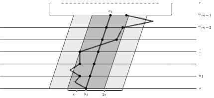
Figure 5.2. On $E_{i}$, the $i^{th}$ path is required to lie within $\epsilon$ of $\ell_{i,u_{m-1}}(u_{j})$ at the times $\{u_{j}:j\in[m-1]\}$. Between these times, the path is required to remain inside the larger cylinder of radius $2\epsilon$ (the union of the light and dark grey regions) around $\ell_{i,v}(\cdot)$ (thick). The points $\ell_{i,u_{m-1}}(u_{j})$ and some admissible values of $X_{u_{j}}^{i}$ are marked as bullets. An inadmissible path between these values (due to exiting the cylinder between $u_{m-2}$ and $u_{m-1}$) is drawn as a zigzag. In order to exit in this way, the path between $X_{u_{j-1}}^{i}$ and $X_{u_{j}}^{i}$ deviates from the straight line between those points by more than $\epsilon$.

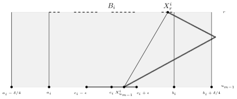
Figure 5.3. By Lemma 4.2, $X_{u_{m-1}}^{i}\in(c_{i}-\epsilon,c_{i}+\epsilon)$ (solid at level $u_{m-1}$) and $X_{r}^{i}\in B_{i}$ (dashed, at level $r$) with positive probability. If $\epsilon$ is such that $(c_{i}-\epsilon,c_{i}+\epsilon)\subset[a_{i},b_{i}]$, then in order to exit the interval $[a_{i}-\delta/4,b_{i}+\delta/4]$, the path must deviate by more than $\delta/4$ from the straight line connecting $X_{u_{m-1}}^{i}$ and $X_{r}^{i}$ on the time interval $[u_{m-1},r]$.

The strict positivity of the infimum follows because the probability being minimized is positive for each $x$ and continuous in $x$. Continuity can be seen either by applying dominated convergence to the integral form of the probability or abstractly as a consequence of the strong Feller property of Brownian bridge. We have

$$Q^{\beta}_{(s,y_{i}),(t;\zeta)}(E_{i})=\frac{1}{Z_{\beta}(t;\zeta\hskip 0.7pt|\hskip 0.7pts,y_{i})}{\int_{\operatorname{\mathbb{R}}}Z_{\beta}(t,x\hskip 0.7pt|\hskip 0.7pts,y_{i})Q^{\beta}_{(s,y),(t,x)}(E_{i})\zeta(dx)}$$

$$\qquad\geq\frac{C^{\prime}\zeta[-K,K]}{(1+2K)^{m}Z_{\beta}(t;\zeta\hskip 0.7pt|\hskip 0.7pts,y_{i})}$$

$$\qquad\qquad\quad\times\;\inf_{x\in[-K,K]}\Big{\{}Z_{\beta}(t,x\hskip 0.7pt|\hskip 0.7pts,y_{i})\mathbf{P}^{BB}_{(s,y_{i}),(t,x)}\big{[}X_{r}^{i}\in B_{i}\,;\forall j\in[m]:|X_{u_{j}}-\ell_{i}(u_{j})|<\epsilon\big{]}\Big{\}}.$$

Now, notice that by construction, we have $|y_{i}-y_{j}|>8\epsilon$ and $|c_{i}-c_{j}|>\delta+4\epsilon>8\epsilon$. Therefore $|\ell_{i,u_{m-1}}(u)-\ell_{j,u_{m-1}}(u)|>8\epsilon$ for all $u\in[s,u_{m-1}]$ and so the tubes in Figure 5.1, which the event $E_{i}$ forces the path to remain in, do not intersect up to time $u_{m-1}$. By hypothesis, we also have $a_{i}-b_{i-1}\geq\delta$ and so the tubes also do not intersect on $[u_{m-1},r]$. Consequently, by independence,

$$Q^{\beta}_{(s,y_{1},\dots,y_{n}),(t;\zeta)}(X^{i}_{r}\in B_{i},i\in[n],\tau_{s:t}^{(n)}>r)$$

$$\qquad\geq Q^{\beta}_{(s,y_{1},\dots,y_{n}),(t;\zeta)}(E_{1},\dots,E_{n})=\prod_{i=1}^{n}Q^{\beta}_{(s,y_{i}),(t;\zeta)}\big{(}E_{i}\big{)}>0.$$

Now, consider $(a_{1},\dots,a_{n}),(b_{1},\dots,b_{n})\in\operatorname{\mathbb{W}}_{n}$ with $a_{i-1}<b_{i-1}<a_{i}$ for $i\in\{2,\dots,n\}$ and call $B_{i}=(a_{i},b_{i})$. The previous result implies that

$$\bigg{\{}(z_{1},\dots,z_{n})\in\operatorname{\mathbb{W}}_{n}:\det_{1\leq i,j\leq n}\bigg{[}\frac{Z_{\beta}(t;\zeta|r,z_{i})Z_{\beta}(r,z_{i}\hskip 0.7pt|\hskip 0.7pts,y_{j})}{Z_{\beta}(t;\zeta\hskip 0.7pt|\hskip 0.7pts,y_{j})}\bigg{]}=0\bigg{\}}\bigcap\,(B_{1}\times\dots,\times B_{n})$$

has Lebesgue measure zero, with a similar result for the other determinant in (ii). By (5.5), it follows that for all $(x_{1},\dots,x_{n})$, $(y_{1},\dots,y_{n})\in\operatorname{\mathbb{W}}_{n}$, the Lebesgue measure of the sets

$$\bigg{\{}(z_{1},\dots,z_{n})\in\operatorname{\mathbb{W}}_{n}:\det_{1\leq i,j\leq n}\big{[}Z_{\beta}(r,z_{j}\hskip 0.7pt|\hskip 0.7pts,y_{i})\big{]}=0\bigg{\}}\text{ and }$$

$$\bigg{\{}(z_{1},\dots,z_{n})\in\operatorname{\mathbb{W}}_{n}:\det_{1\leq i,j\leq n}\big{[}Z_{\beta}(t,x_{j}|r,z_{i})\big{]}=0\bigg{\}}$$

are both zero.

For a permutation $\sigma\in S_{n}$, set $\operatorname{\mathbb{W}}_{n}^{\sigma}=\{z_{1:n}\in\mathbb{R}^{n}:z_{\sigma(1)}<\dotsm<z_{\sigma(n)}\}$. By the Chapman-Kolmogorov identity in Lemma 3.12 and the Cauchy-Binet-Andréief identity, [4, Lemma 3.2.3]), for any $(y_{1},\dots,y_{n})$, $(x_{1},\dots,x_{n})\in\operatorname{\mathbb{W}}_{n}$ and any $s<r<t$,

$$\det_{1\leq i,j\leq n}\bigl{[}Z_{\beta}(t,y_{j}\hskip 0.7pt|\hskip 0.7pts,x_{i})\bigr{]}=\det_{1\leq i,j\leq n}\biggl{[}\int_{\mathbb{R}}Z_{\beta}(t,y_{j}\hskip 0.7pt|\hskip 0.7ptr,z)\hskip 0.9ptZ_{\beta}(r,z\hskip 0.7pt|\hskip 0.7pts,x_{i})\hskip 0.9ptdz\biggr{]}$$

$$=\frac{1}{n!}\int_{\mathbb{R}^{n}}\det_{1\leq i,j\leq n}\bigl{[}Z_{\beta}(t,y_{j}\hskip 0.7pt|\hskip 0.7ptr,z_{i})\bigr{]}\hskip 0.9pt\det_{1\leq i,j\leq n}\bigl{[}Z_{\beta}(r,z_{i}\hskip 0.7pt|\hskip 0.7pts,x_{j})\bigr{]}\hskip 0.9ptdz_{1:n}$$

$$=\frac{1}{n!}\sum_{\sigma\in S_{n}}\int_{\operatorname{\mathbb{W}}_{n}^{\sigma}}\det_{1\leq i,j\leq n}\bigl{[}Z_{\beta}(t,y_{j}\hskip 0.7pt|\hskip 0.7ptr,z_{i})\bigr{]}\hskip 0.9pt\det_{1\leq i,j\leq n}\bigl{[}Z_{\beta}(r,z_{i}\hskip 0.7pt|\hskip 0.7pts,x_{j})\bigr{]}\hskip 0.9ptdz_{1:n}$$

$$=\frac{1}{n!}\sum_{\sigma\in S_{n}}\int_{\operatorname{\mathbb{W}}_{n}^{\sigma}}\det_{1\leq i,j\leq n}\bigl{[}Z_{\beta}(t,y_{j}\hskip 0.7pt|\hskip 0.7ptr,z_{\sigma(i)})\bigr{]}\hskip 0.9pt\det\bigl{[}Z_{\beta}(r,z_{\sigma(i)}\hskip 0.7pt|\hskip 0.7pts,x_{j})\bigr{]}\hskip 0.9ptdz_{1:n}$$

$$=\frac{1}{n!}\sum_{\sigma\in S_{n}}\int_{\operatorname{\mathbb{W}}_{n}}\det_{1\leq i,j\leq n}\bigl{[}Z_{\beta}(t,y_{j}\hskip 0.7pt|\hskip 0.7ptr,z_{i})\bigr{]}\hskip 0.9pt\det_{1\leq i,j\leq n}\bigl{[}Z_{\beta}(r,z_{i}\hskip 0.7pt|\hskip 0.7pts,x_{j})\bigr{]}\hskip 0.9ptdz_{1:n}$$

$$=\int_{\operatorname{\mathbb{W}}_{n}}\det_{1\leq i,j\leq n}\bigl{[}Z_{\beta}(t,y_{j}\hskip 0.7pt|\hskip 0.7ptr,z_{i})\bigr{]}\hskip 0.9pt\det_{1\leq i,j\leq n}\bigl{[}Z_{\beta}(r,z_{i}\hskip 0.7pt|\hskip 0.7pts,x_{j})\bigr{]}\hskip 0.9ptdz_{1:n}>0,$$

by the previous observation. ∎

Proof of Proposition 2.18.

It suffices to check stochastic monotonicity for the finite dimensional distributions. By Proposition 5.2 (ii), for all $s<r<t$, all $\beta\in\operatorname{\mathbb{R}}$, all $\zeta\in\operatorname{\mathcal{M}}_{{\scriptscriptstyle\textrm{HE}}}$, all $y_{1}<y_{2}$ and all $z_{1}<z_{2}$, we have

$$\frac{Z_{\beta}(t;\zeta|r,z_{1})Z_{\beta}(r,z_{1}\hskip 0.7pt|\hskip 0.7pts,y_{1})}{Z_{\beta}(t;\zeta\hskip 0.7pt|\hskip 0.7pts,y_{1})}\frac{Z_{\beta}(t;\zeta|r,z_{2})Z_{\beta}(r,z_{2}\hskip 0.7pt|\hskip 0.7pts,y_{2})}{Z_{\beta}(t;\zeta\hskip 0.7pt|\hskip 0.7pts,y_{2})}$$

$$\qquad\qquad>\frac{Z_{\beta}(t;\zeta|r,z_{1})Z_{\beta}(r,z_{1}\hskip 0.7pt|\hskip 0.7pts,y_{2})}{Z_{\beta}(t;\zeta\hskip 0.7pt|\hskip 0.7pts,y_{2})}\frac{Z_{\beta}(t;\zeta|r,z_{2})Z_{\beta}(r,z_{2}\hskip 0.7pt|\hskip 0.7pts,y_{1})}{Z_{\beta}(t;\zeta\hskip 0.7pt|\hskip 0.7pts,y_{1})}$$

For any $a\in\operatorname{\mathbb{R}}$, integrating both sides of this expression on $(-\infty,a)$ with respect to $z_{1}$ and on $(a,\infty)$ with respect to $z_{2}$, we have

$$Q^{\beta}_{(s,y_{1}),(t;\zeta)}\big{(}X_{r}<a\big{)}Q^{\beta}_{(s,y_{2}),(t;\zeta)}\big{(}X_{r}\geq a\big{)}>Q^{\beta}_{(s,y_{2}),(t;\zeta)}(X_{r}<a)Q^{\beta}_{(s,y_{1}),(t;\zeta)}(X_{r}\geq a)$$

All of the probabilities above here are strictly positive, so we may re-write this as

$$\frac{Q^{\beta}_{(s,y_{2}),(t;\zeta)}(X_{r}\geq a)}{1-Q^{\beta}_{(s,y_{2}),(t;\zeta)}(X_{r}\geq a)}>\frac{Q^{\beta}_{(s,y_{1}),(t;\zeta)}(X_{r}\geq a)}{1-Q^{\beta}_{(s,y_{1}),(t;\zeta)}(X_{r}\geq a)},$$

which holds if and only if

$$Q^{\beta}_{(s,y_{2}),(t;\zeta)}(X_{r}\geq a)>Q^{\beta}_{(s,y_{1}),(t;\zeta)}(X_{r}\geq a).$$

We prove stochastic monotonicity of the $n$-point distributions by induction. Assume that for all $s<t$, all $\zeta\in\operatorname{\mathcal{M}}_{{\scriptscriptstyle\textrm{HE}}}$, all $y_{1}<y_{2}$, all $a_{1:n}\in\mathbb{R}^{n}$, and all $r_{1:n}\in\operatorname{\mathbb{R}}^{n}$ satisfying $s<r_{1}<\dots<r_{n}<t$, we have

$$Q^{\beta}_{(s,y_{2}),(t;\zeta)}(X_{r_{1}}\geq a_{1},\dots,X_{r_{n}}>a_{n})>Q^{\beta}_{(s,y_{1}),(t;\zeta)}(X_{r_{1}}\geq a_{1},\dots,X_{r_{n}}\geq a_{n})$$

Now, fix $a_{1:n+1}\in\operatorname{\mathbb{R}}^{n+1}$ and $r_{1:n+1}$ with $r_{1}<\dots<r_{n}<r_{n+1}$. The induction hypothesis implies that for each $y\in\operatorname{\mathbb{R}}$,

$$z\mapsto Q^{\beta}_{(s,y),(r_{n+1},z)}(X_{r_{1}}\geq a_{1},\dots,X_{r_{n}}\geq a_{n})\mbox{\mymathbb{1}}_{\{z\geq a_{n+1}\}}$$

is non-decreasing. We have

$$Q^{\beta}_{(s,y_{2}),(t;\zeta)}(X_{r_{1}}\geq a_{1},\dots,X_{r_{n}}\geq a_{n},X_{r_{n+1}}\geq a_{n+1})$$

$$=\operatorname{E}_{(s,y_{2}),(t;\zeta)}^{Q^{\beta}}[Q^{\beta}_{(s,y_{2}),(r_{n+1},X_{r_{n+1}})}(X_{r_{1}}\geq a_{1},\dots,X_{r_{n}}\geq a_{n})\mbox{\mymathbb{1}}_{\{X_{r_{n+1}}\geq a_{n+1}\}}]$$

$$\geq\operatorname{E}_{(s,y_{2}),(t;\zeta)}^{Q^{\beta}}[Q^{\beta}_{(s,y_{1}),(r_{n+1},X_{r_{n+1}})}(X_{r_{1}}\geq a_{1},\dots,X_{r_{n}}\geq a_{n})\mbox{\mymathbb{1}}_{\{X_{r_{n+1}}\geq a_{n+1}\}}]$$

$$\geq\operatorname{E}_{(s,y_{1}),(t;\zeta)}^{Q^{\beta}}[Q^{\beta}_{(s,y_{1}),(r_{n+1},X_{r_{n+1}})}(X_{r_{1}}\geq a_{1},\dots,X_{r_{n}}\geq a_{n})\mbox{\mymathbb{1}}_{\{X_{r_{n+1}}\geq a_{n+1}\}}]$$

$$=Q^{\beta}_{(s,y_{1}),(t;\zeta)}(X_{r_{1}}\geq a_{1},\dots,X_{r_{n}}\geq a_{n},X_{r_{n+1}}\geq a_{n+1}),$$

where in the first inequality, we apply the induction hypothesis and in the second, we applied the base case of the induction with $r=r_{n+1}$. This implies the first inequality in (2.14). The second is similar. ∎

Appendix A Mild solutions and uniqueness

In this section we discuss some details and partially survey the literature concerning existence and uniqueness of mild solutions to (1.2) with possibly random initial conditions. We then show that under the most general hypotheses for uniqueness that we identified in the literature, the superposition formulation of $Z_{\beta}(t,x\hskip 0.7pt|\hskip 0.7pts;\mu)$ is, up to indistinguishability, the usual mild solution to (1.2).

Let $X$ be a random variable taking values in the space of positive Borel measures satisfying $\operatorname{\mathbb{P}}(X\in\operatorname{\mathcal{M}}_{{\scriptscriptstyle\textrm{HE}}})=1$ and which is independent of the white noise after some initial time $s$, which we will typically take to be zero. For such $s$, define $\operatorname{\mathcal{F}}^{W,X}_{s,t}=\wedge_{a<s\leq t<b}\hskip 1.1pt\sigma(\operatorname{\mathcal{F}}^{W,0}_{a,b},X)$ to be the augmentation of the natural filtration of the white noise enlarged by $\sigma(X)$. Setting $W_{0}(g)=0$ for all $g\in L^{2}(\operatorname{\mathbb{R}})$ and $W_{t}(g)-W_{s}(g)=W(f_{s,t,g})$, where $f_{s,t,g}(r,x)=\mbox{\mymathbb{1}}_{[s,t]}(r)g(x)$ and $-\infty<s\leq t<\infty$, it is straightforward to check that $W_{t}({\raisebox{1.3pt}{\hskip 0.6pt\scaleobj{0.55}{\bullet}\hskip 0.75pt}})$ defines an orthogonal martingale measure for $t\geq 0$ in the sense of [51] with respect to either $\operatorname{\mathcal{F}}^{W}_{0,t}$ or $\operatorname{\mathcal{F}}^{W,X}_{0,t}$. See the discussion in Chapter 2 of [51].

For each $s\in\operatorname{\mathbb{R}}$, the mild formulation of (1.2) seeks fixed points $U$ to the Duhamel equation

(A.1) $$U(t,x) =\int_{\operatorname{\mathbb{R}}}\rho(t,x-z)X(dz)+\beta\int_{s}^{t}\int_{\operatorname{\mathbb{R}}}\rho(t-r,x-z)U(r,z)W(dz\,dr)$$

which take values in an appropriate class of functions on $\{(t,x)\in\operatorname{\mathbb{R}}^{2}:t>s\}$, where the stochastic integral is understood in the sense of Walsh [51]. Naturally, one needs to impose measurability and integrability conditions on the functions being considered in order to make sense of that stochastic integral. We are only considering processes which have already been shown to exist and to have unique continuous and adapted modifications. We wish to show that this process is our $Z_{\beta}(t,x\hskip 0.7pt|\hskip 0.7pts;X)$, up to indistinguishability. Because our candidate solutions are continuous and adapted by Theorem 2.6, we restrict to this class. This condition is much stricter than necessary, but suffices for our purposes and simplifies the discussion.

Various hypotheses for existence and conditions for uniqueness of solutions have appeared in the literature. For non-random initial data, the minimal assumption that has been studied is that of [11, 12], who assume that

(A.2) $$X\text{ is a non-random measure in }\operatorname{\mathcal{M}}_{{\scriptscriptstyle\textrm{HE}}}.$$

The first paper to allow for random initial data was [6], who assume that there exists a random variable $X_{0}\in\operatorname{\mathcal{C}}(\operatorname{\mathbb{R}},\operatorname{\mathbb{R}})$ so that for each $p>0$, there exists $a_{p}>0$ for which

(A.3) $$X(dx)=X_{0}(x)dx\text{ and }\sup_{r\in\operatorname{\mathbb{R}}}e^{-a_{p}|r|}\operatorname{\mathbb{E}}[|X_{0}(r)|^{p}]<\infty.$$

The first paper we are aware of to systematically study mild solutions of (A.1) was [5]. The results in [5] are stated and proven only under the assumption that for all $t>0$,

(A.4) $$X\text{ is non-random and }\sup_{r\in(0,t]}\sup_{x\in\operatorname{\mathbb{R}}}\sqrt{r}\bigg{(}\int_{\operatorname{\mathbb{R}}}\rho(r,x-z)X(dz)\bigg{)}^{2}<\infty.$$

We begin by recalling this original result. Note that in all of the following statements, we are appealing to translation invariance of the model to extend these results from the case of $s=0$ to $s\in\operatorname{\mathbb{R}}$.

Theorem A.1.

([5, Theorem 3.1]) Under Condition (A.4), for each $s\in\mathbb{R}$ there exists an $(\operatorname{\mathcal{F}}^{W}_{s,t}:s\leq t)$ adapted solution $U\in\operatorname{\mathcal{C}}((s,\infty)\times\operatorname{\mathbb{R}},\operatorname{\mathbb{R}})$ to (A.1) satisfying for all $T>s$,

(A.5) $$\sup_{t\in(s,T]}\sup_{x\in\operatorname{\mathbb{R}}}\int_{s}^{t}\int_{s}^{r}\int_{\operatorname{\mathbb{R}}}\int_{\operatorname{\mathbb{R}}}\rho(t-r,x-y)^{2}\rho(r-v,y-z)^{2}\operatorname{\mathbb{E}}[U(v,z)^{2}]dzdydvdr<\infty.$$

Moreover, under (A.4), if $U$ and $V$ are any two solutions satisfying (A.1) and (A.5), then $U$ and $V$ are indistinguishable.

As mentioned in Remark 1 of [5], the methods employed there can be used to prove a result similar to Theorem A.1 for certain random initial conditions. It is recorded, for example, in Proposition 2.5 in the survey [13], that one can use similar methods to obtain existence and uniqueness of continuous and adapted solutions under the following moment hypothesis on a random initial condition $X$ satisfying the hypotheses above: for all $t>0$,

(A.6) $$\sup_{r\in(0,t]}\sup_{x\in\operatorname{\mathbb{R}}}\operatorname{\mathbb{E}}\bigg{[}\sqrt{r}\bigg{(}\int_{\operatorname{\mathbb{R}}}\rho(r,x-z)X(dz)\bigg{)}^{2}\bigg{]}<\infty.$$

The resulting uniqueness of solutions to (A.1) then also holds among the class of processes satisfying (A.5). We could not find a full proof of this result in the literature, however. We also note that there is a vast literature studying generalizations of (A.1) which imply existence and uniqueness of mild solutions to (A.1) under varying conditions.

The most general existence and uniqueness result we identified in the literature for non-random initial data is the following result, which comes from combining results in [11] and [12].

Theorem A.2.

([12, Theorem 2.4] with [11, Theorem 3.1]) Under Condition (A.2), for each $s\in\mathbb{R}$, there exists an $(\operatorname{\mathcal{F}}^{W}_{s,t}:s\leq t)$ adapted solution $U\in\operatorname{\mathcal{C}}((s,\infty)\times\operatorname{\mathbb{R}},\operatorname{\mathbb{R}})$ to (A.1) satisfying

1. For all $t>s$ and $x\in\operatorname{\mathbb{R}}$,

   $$\int_{s}^{t}\int_{\operatorname{\mathbb{R}}}\rho(t-r,x-z)\operatorname{\mathbb{E}}[U(r,z)^{2}]dzdr<\infty$$

2. For all $t>s$,

   $$\lim_{\begin{subarray}{c}(u,v)\to(t,x)\\ u>s\end{subarray}}\operatorname{\mathbb{E}}\bigg{[}\bigg{(}\int_{s}^{u}\int_{\operatorname{\mathbb{R}}}\rho(u-r,v-z)U(r,z)W(dz\,dr)$$

   $$\qquad\qquad\qquad-\int_{s}^{t}\int_{\operatorname{\mathbb{R}}}\rho(t-r,x-z)U(r,z)W(dz\,dr)\bigg{)}^{2}\bigg{]}=0$$

Moreover, if $U$ and $V$ are any two solutions satisfying these properties, then $U$ and $V$ are indistinguishable.

Both the results in [11, 12] and [5] apply to show the existence and uniqueness of a solution to (2.2) for fixed initial conditions $s,y$, which we record in the following lemma below. The claim about the solution being represented by (2.3) is sketched in Section 3.2 of [1]. This essentially follows from Picard iteration; a pedagogical proof appears in the lecture notes [15, Theorem 2.2].

Lemma A.3.

For each $s,y\in\operatorname{\mathbb{R}}$, there exists a unique (up to indistinguishability) $(\operatorname{\mathcal{F}}^{W,X}_{s,t}:s\leq t)$-adapted process $Z_{\beta}({\raisebox{1.3pt}{\hskip 0.6pt\scaleobj{0.55}{\bullet}\hskip 0.75pt}},{\raisebox{1.3pt}{\hskip 0.6pt\scaleobj{0.55}{\bullet}\hskip 0.75pt}}\hskip 0.7pt|\hskip 0.7pts,y)$ taking values in $\operatorname{\mathcal{C}}((s,\infty),\operatorname{\mathbb{R}})$ which satisfies the mild equation (2.2) and the conditions in either Theorem A.1 or A.2. Moreover, this process is a modification of the process defined for fixed $(s,y,t,x,\beta)\in\operatorname{\mathbb{R}}_{{\scaleobj{0.8}{\uparrow}}}^{4}\times\operatorname{\mathbb{R}}$ by (2.3).

We next turn to the assumption in (A.3), which allows for a class of random initial data which is rich enough to include the exponential of Brownian Motion with drift. These correspond to the (increment-) stationary distributions of the KPZ equation. See [23].

Theorem A.4.

[6, Theorem 3.1] Under Condition (A.3), for each $s\in\mathbb{R}$, there exists an $(\operatorname{\mathcal{F}}^{W,X}_{s,t}:s\leq t)$ adapted process $U(t,x)$ taking values in $\operatorname{\mathcal{C}}([s,\infty),\operatorname{\mathbb{R}})$ which satisfies the mild equation (A.1). For each $T>s$, there exists a constant $a>0$ so that resulting process satisfies

(A.7) $$\sup_{t\in[s,T]}\sup_{x\in\operatorname{\mathbb{R}}}e^{-a|x|}\operatorname{\mathbb{E}}[|U(t,x)|^{2}]<\infty.$$

Moreover, if $U$ and $V$ are two such continuous and adapted solutions satisfying (A.1) and (A.7), then $\operatorname{\mathbb{P}}(U(t,x)=V(t,x)\text{ for all }t>s,x\in\operatorname{\mathbb{R}})=1.$

With the previous results in mind, we now show that $Z_{\beta}(t,x\hskip 0.7pt|\hskip 0.7pts;X)$ defined through (1.3) agrees with the mild solution in (A.1) in the previous results.

Lemma A.5.

Assume that $X$ satisfies either (A.2) or (A.3). For each $s\in\mathbb{R}$, up to indistinguishability, $Z_{\beta}({\raisebox{1.3pt}{\hskip 0.6pt\scaleobj{0.55}{\bullet}\hskip 0.75pt}},{\raisebox{1.3pt}{\hskip 0.6pt\scaleobj{0.55}{\bullet}\hskip 0.75pt}}|s;X)$ (as defined by (1.3)) is the unique continuous and adapted solution to (A.1) in Theorems A.2 and A.4 respectively.

Proof.

Because mild solutions are formulated for fixed initial conditions and fixed $\beta$, scaling and translation invariance implies that it is without loss of generality to consider the case of $\beta=1$ and $s=0$. By construction, $Z_{1}(t,x|0;X)$ is adapted and continuous, so we just need to check that it solves the mild equation and the moment conditions of the two theorems. To check that $Z_{1}(t,x|0;X)$ satisfies (A.1), we will apply the stochastic Fubini theorem; see [18, Theorem 4.33] or [51, Theorem 2.6]. This result shows that whenever

$$\int_{0}^{t}\int_{\operatorname{\mathbb{R}}}\int_{\operatorname{\mathbb{R}}}\rho(t-r,x-z)^{2}\operatorname{\mathbb{E}}[Z_{1}(r,z|0,y)^{2}]X(dy)dzdr<\infty,\text{ if }\eqref{eq:CDcond}\text{ holds or}$$

$$\int_{0}^{t}\int_{\operatorname{\mathbb{R}}}\int_{\operatorname{\mathbb{R}}}\rho(t-r,x-z)^{2}\operatorname{\mathbb{E}}[Z_{1}(r,z|0,y)^{2}]\operatorname{\mathbb{E}}[X_{0}(y)^{2}]dydzdr<\infty\text{ if }\eqref{eq:BGcond}\text{ holds,}$$

we have

$$Z_{1}(t,x|0;X) =\int_{\operatorname{\mathbb{R}}}Z_{1}(t,x|0,y)X(dy)$$

$$=\int_{\operatorname{\mathbb{R}}}\rho(t,x-y)X(dy)+\int_{0}^{t}\int_{\operatorname{\mathbb{R}}}\rho(t-r,x-z)\int_{\operatorname{\mathbb{R}}}Z_{1}(r,z|0,y)X(dy)W(dzdr)$$

$$=\int_{\operatorname{\mathbb{R}}}\rho(t,x-y)X(dy)+\int_{0}^{t}\int_{\operatorname{\mathbb{R}}}\rho(t-r,x-z)Z_{1}(r,z|0;X)W(dzdr).$$

Recall that we have $\operatorname{\mathbb{E}}[Z_{1}(r,z|0,y)^{2}]\leq D_{2,t}\rho(t,z-y)^{2}$. Considering that $\operatorname{\mathbb{E}}[X_{0}(y)^{2}]dy\in\operatorname{\mathcal{M}}_{{\scriptscriptstyle\textrm{HE}}}$, it suffices to consider the first integral under (A.2). By Lemma C.2,

$$\int_{\operatorname{\mathbb{R}}}\int_{0}^{t}\int_{\operatorname{\mathbb{R}}}\rho(t-r,x-z)^{2}\rho(r,z-y)^{2}dzdrX(dy) =\frac{\sqrt{\pi t}}{2}\int_{\operatorname{\mathbb{R}}}\rho(t,x-y)X(dy),$$

which is finite by hypothesis. It remains to check the moment hypotheses. Call $V(t,x)=Z_{1}(t,x|0,X)$, so that $V(t,x)$ solves (A.1). Under (A.3), by Cauchy-Schwarz applied twice

$$\operatorname{\mathbb{E}}[V(t,x)^{2}]=\int_{\operatorname{\mathbb{R}}}\int_{\operatorname{\mathbb{R}}}\operatorname{\mathbb{E}}\bigg{[}Z_{1}(t,x|0,z)Z_{1}(t,x|0,w)\bigg{]}\operatorname{\mathbb{E}}[X_{0}(w)X_{0}(z)]dzdw$$

$$\leq CD_{2,t}\int_{\operatorname{\mathbb{R}}}\int_{\operatorname{\mathbb{R}}}\rho(t,x-z)\rho(t,x-w)e^{\frac{a_{2}}{2}(|w|+|z|)}dwdz$$

$$\leq CD_{2,t}\bigg{(}\int_{\operatorname{\mathbb{R}}}\rho(t,x-z)(e^{\frac{a_{2}}{2}z}+e^{-\frac{a_{2}}{2}z})dz\bigg{)}^{2}=CD_{2,t}\bigg{(}e^{\frac{a_{2}}{2}x+\frac{a_{2}^{2}}{8}t}+e^{-\frac{a_{2}}{2}x+\frac{a_{2}^{2}}{8}t}\bigg{)}^{2},$$

where $C$ is the value of the supremum appearing in (A.3). This verifies (A.7).

Next, we turn to showing conditions (i) and (ii) in Theorem A.2 under (A.4). We have

$$\int_{0}^{t}\int_{\operatorname{\mathbb{R}}}\rho(t-r,x-z)\operatorname{\mathbb{E}}[V(r,z)^{2}]dzdr$$

$$\leq D_{2,t}\int_{0}^{t}\int_{\operatorname{\mathbb{R}}}\rho(t-r,x-z)\bigg{(}\int_{\operatorname{\mathbb{R}}}\rho(r,z-y)X(dy)\bigg{)}^{2}dzdr$$

$$=\int_{\operatorname{\mathbb{R}}}\int_{\operatorname{\mathbb{R}}}\int_{0}^{t}\frac{D_{2,t}}{(2\pi)^{3/2}r\sqrt{t-r}}\int_{\operatorname{\mathbb{R}}}e^{-\bigg{[}\frac{(x-z)^{2}}{2(t-r)}+\frac{(z-v)^{2}+(z-w)^{2}}{2r}\bigg{]}}dzdrX(dv)X(dw)$$

$$=\int_{\operatorname{\mathbb{R}}}\int_{\operatorname{\mathbb{R}}}\int_{0}^{t}\frac{D_{2,t}}{(2\pi)^{3/2}r\sqrt{t-r}}\int_{\operatorname{\mathbb{R}}}e^{-\frac{z^{2}}{2}\big{(}\frac{1}{t-r}+\frac{2}{r}\big{)}}e^{z\big{(}\frac{x}{t-r}+\frac{v+w}{r}\big{)}}dze^{-\big{(}\frac{x^{2}}{2(t-r)}+\frac{v^{2}+w^{2}}{2r}\big{)}}drX(dv)X(dw)$$

$$=\int_{\operatorname{\mathbb{R}}}\int_{\operatorname{\mathbb{R}}}\int_{0}^{t}\frac{D_{2,t}}{(2\pi)r\sqrt{t-r}\sqrt{\frac{1}{t-r}+\frac{2}{r}}}e^{\frac{\big{(}\frac{x}{t-r}+\frac{v+w}{r}\big{)}^{2}}{2\big{(}\frac{1}{t-r}+\frac{2}{r}\big{)}}-\big{(}\frac{x^{2}}{2(t-r)}+\frac{v^{2}+w^{2}}{2r}\big{)}}drX(dv)X(dw)$$

$$=\int_{\operatorname{\mathbb{R}}}\int_{\operatorname{\mathbb{R}}}\int_{0}^{t}\frac{D_{2,t}}{2\pi\sqrt{r(r+2(t-r))}}e^{-\frac{x^{2}}{2t-r}+\frac{x(v+w)}{2t-r}-\frac{(t-r)(v-w)^{2}+r(v^{2}+w^{2})}{2r(2t-r)}}drX(dv)X(dw)$$

$$\leq e^{-\frac{x^{2}}{t}}\int_{0}^{t}\frac{D_{2,t}}{2\pi\sqrt{r(r+2(t-r))}}dr\bigg{(}\int_{\operatorname{\mathbb{R}}}e^{\frac{2|x||v|-v^{2}}{2t}}X(dv)\bigg{)}^{2}<\infty.$$

In the last step, we bounded $|x(v+w)|\leq|x|(|v|+|w|)$, $-(t-r)(v-w)^{2}\leq 0$, and then $t\leq 2t-r$. (i) follows.

Still considering the case of (A.2), we now verify condition (ii). For simplicity, we take the case of $u=t+h$, $h>0$, $h\to 0$. The case of $u=t-h$ follows similarly.

$$\operatorname{\mathbb{E}}\bigg{[}\bigg{(}\int_{0}^{u}\int_{\operatorname{\mathbb{R}}}\rho(u-r,v-z)V(r,z)W(dz\,dr)-\int_{0}^{t}\int_{\operatorname{\mathbb{R}}}\rho(t-r,x-z)V(r,z)W(dz\,dr)\bigg{)}^{2}\bigg{]}$$

$$=\operatorname{\mathbb{E}}\bigg{[}\bigg{(}\int_{0}^{t}\int_{\operatorname{\mathbb{R}}}\big{(}\rho(t+h-r,v-z)-\rho(t-r,x-z)\big{)}V(r,z)W(dz\,dr)\bigg{)}^{2}\bigg{]}$$

$$\qquad+\operatorname{\mathbb{E}}\bigg{[}\bigg{(}\int_{t}^{t+h}\int_{\operatorname{\mathbb{R}}}\rho(t+h-r,v-z)V(r,z)W(dz\,dr)\bigg{)}^{2}\bigg{]}$$

$$\leq D_{2,2t}\int_{\operatorname{\mathbb{R}}}\int_{\operatorname{\mathbb{R}}}\big{(}\rho(t+h-r,v-z)-\rho(t-r,x-z)\big{)}^{2}\bigg{(}\int_{\operatorname{\mathbb{R}}}\rho(r,z-w)X(dw)\bigg{)}^{2}\mbox{\mymathbb{1}}_{(0,t)}(r)dz\,dr$$

$$\qquad\qquad+D_{2,2t}\int_{\operatorname{\mathbb{R}}}\int_{\operatorname{\mathbb{R}}}\rho(t+h-r,v-z)^{2}\bigg{(}\int_{\operatorname{\mathbb{R}}}\rho(r,z-w)X(dw)\bigg{)}^{2}\mbox{\mymathbb{1}}_{(t,t+h)}(r)dz\,dr$$

Note that the integrands in both integrals above converge to zero pointwise.We bound

$$\big{(}\rho(t+h-r,v-z)-\rho(t-r,x-z)\big{)}^{2}\bigg{(}\int_{\operatorname{\mathbb{R}}}\rho(r,z-w)X(dw)\bigg{)}^{2}\mbox{\mymathbb{1}}_{(0,t)}(r)$$

(A.8) $$\leq 2\rho(t+h-r,v-z)^{2}\bigg{(}\int_{\operatorname{\mathbb{R}}}\rho(r,z-w)X(dw)\bigg{)}^{2}\mbox{\mymathbb{1}}_{(0,t)}(r)$$

(A.9) $$+2\rho(t-r,x-z)^{2}\bigg{(}\int_{\operatorname{\mathbb{R}}}\rho(r,z-w)X(dw)\bigg{)}^{2}\mbox{\mymathbb{1}}_{(0,t)}(r)$$

By the generalized dominated convergence theorem [49, Theorem 4.17], to show that the first integral converges to zero, it suffices to show that

$$\lim_{\begin{subarray}{c}h\searrow 0\\ v\to x\end{subarray}}\int_{\operatorname{\mathbb{R}}}\int_{\operatorname{\mathbb{R}}}\rho(t+h-r,v-z)^{2}\bigg{(}\int_{\operatorname{\mathbb{R}}}\rho(r,z-w)X(dw)\bigg{)}^{2}\mbox{\mymathbb{1}}_{(0,t)}(r)dz\,dr$$

$$=\int_{\operatorname{\mathbb{R}}}\int_{\operatorname{\mathbb{R}}}\rho(t-r,x-z)^{2}\bigg{(}\int_{\operatorname{\mathbb{R}}}\rho(r,z-w)X(dw)\bigg{)}^{2}\mbox{\mymathbb{1}}_{(0,t)}(r)dz\,dr<\infty$$

Note that there are two claims here: the integral in (A.9) does not depend on $h$ or $v$ and is the limit of the integral in (A.8) as $h\searrow 0$ and $v\to x$. We must show that the integral in (A.9) is finite and that the integral in (A.8) converges to it. Arguing as above, we compute for $h\geq 0$ (now, including the case of (A.9)),

$$\int_{\operatorname{\mathbb{R}}}\int_{\operatorname{\mathbb{R}}}\rho(t+h-r,v-z)^{2}\bigg{(}\int_{\operatorname{\mathbb{R}}}\rho(r,z-w)X(dw)\bigg{)}^{2}\mbox{\mymathbb{1}}_{(0,t)}(r)dz\,dr$$

$$=\int_{\operatorname{\mathbb{R}}}\int_{\operatorname{\mathbb{R}}}\int_{0}^{t}\frac{(2\pi)^{-2}}{(t+h-r)r}\int_{\operatorname{\mathbb{R}}}e^{-\frac{z^{2}}{2}\big{(}\frac{2}{t+h-r}+\frac{2}{r}\big{)}}e^{z\big{(}\frac{2v}{t+h-r}+\frac{y+w}{r}\big{)}}dze^{-\big{(}\frac{2v^{2}}{t+h-r}+\frac{y^{2}+w^{2}}{2r}\big{)}}dr\,X(dy)\,X(dw)$$

$$=\int_{\operatorname{\mathbb{R}}}\int_{\operatorname{\mathbb{R}}}\int_{0}^{t}\frac{(2\pi)^{-{3/2}}}{(t+h-r)r\sqrt{\frac{2}{t+h-r}+\frac{2}{r}}}e^{\frac{\big{(}\frac{2v}{t+h-r}+\frac{y+w}{r}\big{)}^{2}}{2\big{(}\frac{2}{t+h-r}+\frac{2}{r}\big{)}}}e^{-\big{(}\frac{2v^{2}}{t+h-r}+\frac{y^{2}+w^{2}}{2r}\big{)}}dr\,X(dy)\,X(dw)$$

$$=\int_{\operatorname{\mathbb{R}}}\int_{\operatorname{\mathbb{R}}}\int_{0}^{t}\frac{(2\pi)^{-{3/2}}}{\sqrt{2(t+h)r(t+h-r)}}e^{-v^{2}\big{(}\frac{2}{t+h}+\frac{r}{(t+h)(t+h-r)}\big{)}+\frac{v(y+w)}{t+h}-\frac{(w-y)^{2}}{4r}-\frac{(w+y)^{2}}{4(t+h)}}dr\,X(dy)\,X(dw)$$

The integrand is continuous in $h$ and $v$, so to show that this integral converges, we may use the ordinary dominated convergence theorem. For any $h\in[0,t]$ and $v\in[-K,K]$, $r\in(0,t)$ and $y,w\in\operatorname{\mathbb{R}}$, we have

$$\frac{(2\pi)^{-{3/2}}}{\sqrt{2(t+h)r(t+h-r)}}e^{-v^{2}\big{(}\frac{2}{t+h}+\frac{r}{(t+h)(t+h-r)}\big{)}+\frac{v(y+w)}{t+h}-\frac{(y-w)^{2}(t+h-r)}{4r(t+h)}-\frac{y^{2}+w^{2}}{4(t+h)}}$$

$$\leq\frac{1}{\sqrt{t\cdot r\cdot(t-r)}}e^{\frac{|K|(|y|+|w|)}{t}-\frac{y^{2}+w^{2}}{8t}},$$

and

$$\int_{\operatorname{\mathbb{R}}}\int_{\operatorname{\mathbb{R}}}\int_{0}^{t}\frac{1}{\sqrt{t\cdot r\cdot(t-r)}}e^{\frac{|K|(|y|+|w|)}{t}-\frac{y^{2}+w^{2}}{8t}}dr\,X(dy)\,X(dw)<\infty.$$

The result follows. It remains to show that

$$\lim_{\begin{subarray}{c}h\searrow 0\\ v\to x\end{subarray}}\int_{\operatorname{\mathbb{R}}}\int_{\operatorname{\mathbb{R}}}\rho(t+h-r,v-z)^{2}\bigg{(}\int_{\operatorname{\mathbb{R}}}\rho(r,z-w)X(dw)\bigg{)}^{2}\mbox{\mymathbb{1}}_{(t,t+h)}(r)dz\,dr=0,$$

which follows from essentially the same estimates as in the previous case. (ii) now follows. ∎

Appendix B Continuity of stochastic processes

This appendix presents a version of the Kolmogorov-Chentsov theorem sufficient for our purposes. For $d\geq 2$, we consider a process $X$ with values in a complete separable metric space $(S,\varrho)$ and indexed by $d-2$ copies of the unit interval $[0,1]$ and one copy of the time-ordered unit triangle $\operatorname{\mathbf{T}}_{\delta}=\{(s^{1},s^{2}):0\leq s^{1}\leq s^{1}+\delta\leq s^{2}\leq 1\}$ with a gap $\delta\in[0,1)$. The case $\delta=0$ corresponds to enforcing only the ordering $s^{1}\leq s^{2}$. Generic points of $[0,1]^{d-2}\times\operatorname{\mathbf{T}}_{\delta}$ are denoted by $r=(r^{1},\dots,r^{d-2},r^{d-1},r^{d})$, with superscripts for coordinates. The last two coordinates satisfy $r^{d-1}\leq r^{d}-\delta$. Subscripts are reserved for indexing sequences in $[0,1]^{d-2}\times\operatorname{\mathbf{T}}_{\delta}$.

For $n\in\mathbb{Z}_{+}$ let

$$D_{\delta,n}=\bigl{\{}(k^{1},\dotsc,k^{d})2^{-n}\in[0,1]^{d-2}\times\operatorname{\mathbf{T}}_{\delta}:k^{1},\dotsc,k^{d}\in\llbracket 0,2^{n}\rrbracket\bigr{\}}$$

and then $D_{\delta}=\bigcup_{n\in\mathbb{Z}_{+}}D_{\delta,n}$, the set of dyadic rational points in $[0,1]^{d-2}\times\operatorname{\mathbf{T}}_{\delta}$.

Theorem B.1.

Fix $d\geq 2$ and $\delta\in[0,1)$ as above and let $(S,\varrho)$ be a complete separable metric space.

(a) Suppose $\{X_{r}:r\in D_{\delta}\}$ is an $S$-valued stochastic process defined on a complete probability space $(\Omega,\mathcal{F},\operatorname{\mathbb{P}})$ with the following property: there exist constants $A<\infty$ and $\alpha_{1},\dotsc,\alpha_{d},\nu>0$ such that

(B.1) $$\operatorname{\mathbb{E}}\bigl{[}\varrho(X_{s},X_{r})^{\nu}\,\bigr{]}\leq A\sum_{i=1}^{d}|s^{i}-r^{i}|^{d+\alpha_{i}}\quad\text{for all $r,s\in D_{\delta}$.}$$

Then there exists an $S$-valued process $\{Y_{s}:s\in[0,1]^{d-2}\times\operatorname{\mathbf{T}}_{\delta}\}$ on $(\Omega,\operatorname{\mathcal{F}},\operatorname{\mathbb{P}})$ such that the path $s\mapsto Y_{s}(\omega)$ is continuous for each $\omega\in\Omega$ and $P\{Y_{s}=X_{s}\}=1$ for each $s\in D_{\delta}$. Furthermore, for all choices of $\sigma_{i}\in(0,\alpha_{i}/\nu)$ for $i\in[d]$,

(B.2) $$E\biggl{[}\hskip 0.9pt\sup_{r\neq s\;\text{\rm in }[0,1]^{d-2}\times\operatorname{\mathbf{T}}_{\delta}}\,\biggl{\lvert}\frac{\varrho(Y_{s}(\omega),Y_{r}(\omega))}{\sum_{i=1}^{d}|s^{i}-r^{i}|^{\sigma_{i}}}\biggr{\rvert}^{\nu}\,\biggr{]}\leq A\left(\sum_{i=1}^{d}\frac{2^{\sigma_{i}+1}}{(1-2^{\sigma_{i}-\alpha_{i}/\nu})(1-2^{-\alpha_{i}/\nu})}\right)^{\nu}<\infty.$$

(b) Suppose $\{X_{s}:s\in[0,1]^{d-2}\times\operatorname{\mathbf{T}}_{\delta}\}$ is an $S$-valued stochastic process that satisfies the moment bound (B.1) for all $r,s\in[0,1]^{d-2}\times\operatorname{\mathbf{T}}_{\delta}$. Then the process $Y$ of part (a) is a version of $X$. If $X$ is almost surely continuous to begin with, then $P\{\hskip 0.7ptY_{s}=X_{s}\,\forall s\in[0,1]^{d-2}\times\operatorname{\mathbf{T}}_{\delta}\hskip 0.7pt\}=1$.

The proof is a standard chaining argument, which we omit.

Appendix C Computations

The following sequence of lemmas present elementary computations that go into our Hölder regularity estimates.

Lemma C.1.

For $t>0$ and $x\in\operatorname{\mathbb{R}}$,

$$\int_{\operatorname{\mathbb{R}}}\frac{\rho(t-r,x-z)^{2}\rho(r,z)^{2}}{\rho^{2}(t,x)}dz=\frac{\sqrt{t}}{2\sqrt{\pi(t-r)r}}\mbox{\mymathbb{1}}_{(0,t)}(r)$$

Proof.

For $0<r<t$,

$$\int_{\operatorname{\mathbb{R}}}\rho(t-r,x-z)^{2}\rho(r,z)^{2}dz =\int_{\operatorname{\mathbb{R}}}\frac{1}{(2\pi)^{2}(t-r)r}e^{-\left[\frac{(x-z)^{2}}{t-r}+\frac{z^{2}}{r}\right]}dz$$

$$=\frac{1}{(2\pi)^{2}(t-r)r}\int_{\operatorname{\mathbb{R}}}e^{-\left[\frac{t}{(t-r)r}\left(z-\frac{\frac{x}{t-r}}{\frac{1}{t-r}+\frac{1}{r}}\right)^{2}+\frac{x^{2}}{t}\right]}dz$$

$$=\frac{1}{(2\pi)^{2}(t-r)r}\sqrt{\frac{\pi(t-r)r}{t}}e^{-\frac{x^{2}}{t}}=\frac{\sqrt{t}}{2\sqrt{\pi(t-r)r}}\rho(t,x)^{2}.\qed$$

Lemma C.2.

For $0<t$ and $x\in\operatorname{\mathbb{R}}$,

$$\int_{0}^{t}\int_{\operatorname{\mathbb{R}}}\frac{\rho(t-r,x-z)^{2}\rho(r,z)^{2}}{\rho(t,x)^{2}}dz\,dr =\frac{\sqrt{t\pi}}{2}$$

Proof.

$$\int_{0}^{t}\int_{\operatorname{\mathbb{R}}}\frac{\rho(t-r,x-z)^{2}\rho(r,z)^{2}}{\rho^{2}(t,x)}dz\,dr =\frac{1}{2\sqrt{\pi}}\int_{0}^{t}\sqrt{\frac{t}{r(t-r)}}dr=\frac{\sqrt{t\pi}}{2}.\qed$$

Lemma C.3.

For $t,h>0$ and $x\in\operatorname{\mathbb{R}}$,

$$\int_{0}^{t}\int_{\operatorname{\mathbb{R}}}\bigg{[}\frac{\rho(t+h-r,x-z)^{2}\rho(r,z)^{2}}{\rho^{2}(t+h,x)}\bigg{]}dz\,dr=\frac{\sqrt{t+h}}{2\sqrt{\pi}}\bigg{[}\arcsin\left(1-\frac{2h}{t+h}\right)+\frac{\pi}{2}\bigg{]}$$

Proof.

By Lemma C.2,

$$\int_{0}^{t}\int_{\operatorname{\mathbb{R}}}\bigg{[}\frac{\rho(t+h-r,x-z)^{2}\rho(r,z)^{2}}{\rho^{2}(t+h,x)}\bigg{]}dz\,dr =\int_{0}^{t}\frac{\sqrt{t+h}}{2\sqrt{\pi(t+h-r)r}}dr$$

$$=\frac{\sqrt{t+h}}{2\sqrt{\pi}}\bigg{[}\arcsin\left(\frac{t-h}{t+h}\right)+\frac{\pi}{2}\bigg{]}.\qed$$

Lemma C.4.

For $t,h>0$ and $x\in\operatorname{\mathbb{R}}$,

$$\int_{t}^{t+h}\int_{\operatorname{\mathbb{R}}}\bigg{[}\frac{\rho(t+h-r,x-z)^{2}\rho(r,z)^{2}}{\rho^{2}(t+h,x)}\bigg{]}dz\,dr =\frac{\sqrt{t+h}}{2\sqrt{\pi}}\bigg{[}\frac{\pi}{2}-\arcsin\left(1-\frac{2h}{t+h}\right)\bigg{]}\leq 4\sqrt{h}.$$

Proof.

By Lemma C.3,

$$\int_{t}^{t+h}\int_{\operatorname{\mathbb{R}}}\frac{\rho(t+h-r,x-z)^{2}\rho(r,z)^{2}}{\rho^{2}(t+h,x)}dz\,dr=\int_{t}^{t+h}\frac{\sqrt{t+h}}{2\sqrt{\pi}\sqrt{(t+h-r)r}}dr$$

$$=\frac{1}{2\sqrt{\pi}}\int_{t}^{t+h}dr\frac{\sqrt{t+h}}{\sqrt{(t+h-r)r}}=\frac{\sqrt{t+h}}{2\sqrt{\pi}}\int_{\frac{t}{t+h}}^{1}du\frac{1}{\sqrt{u(1-u)}}$$

$$=\frac{\sqrt{t+h}}{\sqrt{\pi}}\int_{\frac{t}{t+h}}^{1}du\frac{1}{\sqrt{1-(2u-1)^{2}}}=\frac{\sqrt{t+h}}{2\sqrt{\pi}}\int_{\frac{t-h}{t+h}}^{1}dv\frac{1}{\sqrt{1-v^{2}}}$$

$$=\frac{\sqrt{t+h}}{2\sqrt{\pi}}\bigg{[}\frac{\pi}{2}-\arcsin\left(\frac{t-h}{t+h}\right)\bigg{]}$$

For the inequality, we observe that for $x\in(0,2)$, $\frac{\pi}{2}-\arcsin\left(1-x\right)<8\sqrt{x}$. This can be verified by observing that the two functions are equal at $0$ and the derivatives remain ordered on $(0,2)$. Writing $(t-h)/(t+h)=1-2h/(t+h)$, we have

$$\frac{\sqrt{t+h}}{2\sqrt{\pi}}\bigg{[}\frac{\pi}{2}-\arcsin\left(1-\frac{2h}{t+h}\right)\bigg{]}\leq\frac{4\sqrt{2h}}{\sqrt{\pi}}\leq 4\sqrt{h}$$

∎

Lemma C.5.

For $0<t$ and $x,y\in\operatorname{\mathbb{R}}$,

$$\frac{\sqrt{\pi t}}{2}-\frac{|x-y|}{2}\leq\int_{0}^{t}\int_{\operatorname{\mathbb{R}}}\bigg{[}\frac{\rho(t-r,y-z)\rho(r,z)}{\rho(t,y)}\frac{\rho(t-r,x-z)\rho(r,z)}{\rho(t,x)}\bigg{]}drdz\leq\frac{\sqrt{\pi t}}{2}$$

Proof.

Notice that for $r\in(0,t)$,

$$\frac{(y-z)^{2}+(z-x)^{2}}{2(t-r)}+\frac{z^{2}}{r} =\left(\frac{t}{r(t-r)}\right)\left(z-\frac{r(x+y)}{2t}\right)^{2}+\frac{x^{2}}{2t}+\frac{y^{2}}{2t}+\frac{r(x-y)^{2}}{4t(t-r)}.$$

Therefore, after changing variables, in the second equality,

$$\int_{\operatorname{\mathbb{R}}}\bigg{[}\frac{\rho(t-r,y-z)\rho(r,z)}{\rho(t,y)}\frac{\rho(t-r,x-z)\rho(r,z)}{\rho(t,x)}\bigg{]}dz$$

$$=\frac{1}{(2\pi)}\frac{t}{r(t-r)}\int_{\operatorname{\mathbb{R}}}e^{\frac{x^{2}+y^{2}}{2t}-\bigg{[}\frac{(y-z)^{2}+(z-x)^{2}}{2(t-r)}+\frac{z^{2}}{r}\bigg{]}}dz$$

$$=\frac{1}{(2\pi)}\frac{t}{r(t-r)}e^{-\frac{(x-y)^{2}r}{4t(t-r)}}\int_{\operatorname{\mathbb{R}}}e^{-\frac{t}{r(t-r)}z^{2}}dz=\frac{1}{2\sqrt{\pi}}\sqrt{\frac{t}{r(t-r)}}e^{-\frac{(x-y)^{2}r}{4t(t-r)}}.$$

To compute the $dr$ integral, we now substitute $s=\frac{r}{t(t-r)}$, which satisfies $r=\frac{st^{2}}{1+st}$.

$$dr=\frac{t^{2}}{(1+st)^{2}}ds,\qquad\frac{t}{t(t-r)}=\frac{(1+st)^{2}}{st^{2}},\qquad dr\sqrt{\frac{t}{r(t-r)}}=ds\frac{t}{\sqrt{s}(1+st)}$$

$$\int_{0}^{t}\frac{1}{2\sqrt{\pi}}\sqrt{\frac{t}{r(t-r)}}e^{-\frac{(x-y)^{2}r}{4t(t-r)}}dr =\frac{t}{2\sqrt{\pi}}\int_{0}^{\infty}\frac{1}{\sqrt{s}(1+st)}e^{-\frac{(x-y)^{2}}{4}s}ds$$

For $\alpha\geq 0$, call

$$I(\alpha) =\frac{t}{2\sqrt{\pi}}\int_{0}^{\infty}ds\frac{1}{\sqrt{s}(1+st)}e^{-\alpha s}.$$

We have $I(0)=\frac{\sqrt{\pi t}}{2}$ and

$$I^{\prime}(\alpha) =\frac{-t}{2\sqrt{\pi}}\int_{0}^{\infty}ds\frac{\sqrt{s}}{1+st}e^{-\alpha s}$$

Substitute $u=\alpha s$ so that

$$\frac{du}{\alpha}=ds,\qquad\frac{\sqrt{s}}{1+st}=\frac{\sqrt{\alpha}\sqrt{u}}{\alpha+ut},\qquad ds\frac{\sqrt{s}}{1+st}=du\frac{1}{\sqrt{\alpha}}\frac{\sqrt{u}}{\alpha+ut}.$$

Then

$$I^{\prime}(\alpha) =\frac{-t}{2\sqrt{\pi}}\int_{0}^{\infty}du\frac{1}{\sqrt{\alpha}}\frac{\sqrt{u}}{\alpha+ut}e^{-u}\geq\frac{-1}{2\sqrt{\pi}}\frac{1}{\sqrt{\alpha}}\int_{0}^{\infty}du\frac{1}{\sqrt{u}}e^{-u}=-\frac{1}{2\sqrt{\alpha}}$$

It follows that

$$\frac{t}{2\sqrt{\pi}}\int_{0}^{\infty}ds\frac{1}{\sqrt{s}(1+st)}e^{-\frac{(x-y)^{2}}{4}s}=I\left(\frac{(x-y)^{2}}{4}\right) \geq\frac{\sqrt{\pi t}}{2}-\frac{|x-y|}{2}.\qed$$

The next result follows from the previous result by expanding out the square.

Corollary C.6.

For $0<t$ and $x,y\in\operatorname{\mathbb{R}}$,

$$\int_{0}^{t}\int_{\operatorname{\mathbb{R}}}\bigg{[}\frac{\rho(t-r,y-z)\rho(r,z)}{\rho(t,y)}-\frac{\rho(t-r,x-z)\rho(r,z)}{\rho(t,x)}\bigg{]}^{2}dzdr\leq|x-y|.$$

Next, we turn to the more difficult case where the heat kernels have different time coordinates, but the same space coordinate. We begin by computing the space integral of the cross-term that will appear when we expand out the square:

Lemma C.7.

For $0<t$, $h>0$, and $x\in\operatorname{\mathbb{R}}$,

$$\int_{\operatorname{\mathbb{R}}}\bigg{[}\frac{\rho(t+h-r,x-z)\rho(r,z)}{\rho(t+h,x)}\frac{\rho(t-r,x-z)\rho(r,z)}{\rho(t,x)}\bigg{]}dz=$$

$$\frac{\sqrt{t(t+h)}}{\sqrt{2\pi r((t+h)(t-r)+t(t+h-r))}}\bigg{[}e^{-\frac{x^{2}}{2t}\frac{h^{2}r}{(t+h)((t+h)(t-r)+t(t+h-r)))}}\bigg{]}\mbox{\mymathbb{1}}_{(0,t)}(r)$$

Proof.

Write

$$\int_{\operatorname{\mathbb{R}}}\bigg{[}\frac{\rho(t+h-r,x-z)\rho(r,z)}{\rho(t+h,x)}\frac{\rho(t-r,x-z)\rho(r,z)}{\rho(t,x)}\bigg{]}dz$$

$$=\frac{1}{(2\pi)}\sqrt{\frac{t+h}{(t+h-r)r}}\sqrt{\frac{t}{(t-r)r}}\int_{\operatorname{\mathbb{R}}}\bigg{[}e^{\frac{x^{2}}{2(t+h)}+\frac{x^{2}}{2t}-\big{(}\frac{(x-z)^{2}}{2(t+h-r)}+\frac{(x-z)^{2}}{2(t-r)}+\frac{z^{2}}{r}\big{)}}\bigg{]}dz\,\mbox{\mymathbb{1}}_{(0,t)}(r)$$

We note that

$$\bigg{[}\frac{1}{2(t+h-r)}+\frac{1}{2(t-r)}\bigg{]}(x-z)^{2}+\frac{1}{r}z^{2}$$

$$=\left(\frac{1}{2(t-r)}+\frac{1}{2(t+h-r)}+\frac{1}{r}\right)\left(z-\frac{\left(\frac{1}{2(t-r)}+\frac{1}{2(t+h-r)}\right)x}{\frac{1}{2(t-r)}+\frac{1}{2(t+h-r)}+\frac{1}{r}}\right)^{2}+\frac{\left(\frac{1}{2(t-r)}+\frac{1}{2(t+h-r)}\right)\frac{1}{r}}{\frac{1}{2(t-r)}+\frac{1}{2(t+h-r)}+\frac{1}{r}}x^{2}.$$

We have

$$\frac{1}{2(t+h-r)}+\frac{1}{2(t-r)}+\frac{1}{r}=\frac{(t+h)(t-r)+t(t+h-r)}{2(t+h-r)(t-r)r},$$

It follows that

$$\int_{\operatorname{\mathbb{R}}}\bigg{[}\frac{\rho(t+h-r,x-z)\rho(r,z)}{\rho(t+h,x)}\frac{\rho(t-r,x-z)\rho(r,z)}{\rho(t,x)}\bigg{]}dz$$

$$=\frac{1}{2\pi}\sqrt{\frac{t+h}{(t+h-r)r}}\sqrt{\frac{t}{(t-r)r}}\sqrt{\frac{2\pi(t+h-r)(t-r)r}{(t+h)(t-r)+t(t+h-r)}}\times$$

$$\qquad\qquad\qquad\bigg{[}e^{\frac{x^{2}}{2(t+h)}+\frac{x^{2}}{2t}-\frac{\left(\frac{1}{2(t-r)}+\frac{1}{2(t+h-r)}\right)\frac{1}{r}}{\frac{1}{2(t-r)}+\frac{1}{2(t+h-r)}+\frac{1}{r}}x^{2}}\bigg{]}\mbox{\mymathbb{1}}_{(0,t)}(r).$$

The remainder of the claim is tedious but easy algebra. ∎

The next result is the point where our results become suboptimal. A more refined analysis is likely possible to improve this estimate if one is interested in optimal Hölder regularity at the boundary, but it suffices for our purposes.

Lemma C.8.

For $\delta<1$, $0<\delta\leq t\leq t+h\leq T$ with $T>1$, and $x\in\operatorname{\mathbb{R}}$,

$$\frac{\sqrt{\pi t}}{2}-\frac{T}{\delta\sqrt{\pi}}\sqrt{h}-h\frac{\sqrt{\pi}T^{3/2}}{8\delta^{3}}x^{2}$$

$$\qquad\qquad\leq\int_{0}^{t}\int_{\operatorname{\mathbb{R}}}\frac{\rho(t+h-r,x-z)\rho(r,z)}{\rho(t+h,x)}\frac{\rho(t-r,x-z)\rho(r,z)}{\rho(t,x)}dzdr\leq\frac{\sqrt{\pi t}}{2}.$$

Proof.

Applying Lemma C.7, we define for $t,x$ as in the statement and $h\in[0,T-t]$,

$$I(h) =\int_{0}^{t}\int_{\operatorname{\mathbb{R}}}\bigg{[}\frac{\rho(t+h-r,x-z)\rho(r,z)}{\rho(t+h,x)}\frac{\rho(t-r,x-z)\rho(r,z)}{\rho(t,x)}\bigg{]}dzdr$$

$$=\frac{\sqrt{t}}{\sqrt{2\pi}}\int_{0}^{t}\frac{\sqrt{t+h}}{\sqrt{r((t+h)(t-r)+t(t+h-r))}}\bigg{[}e^{-\frac{x^{2}}{2t}\frac{h^{2}r}{(t+h)((t+h)(t-r)+t(t+h-r)))}}\bigg{]}dr$$

Without loss of generality, take $T>t$. Notice that for all $h>0$,

$$I(h)\leq I(0)=\frac{\sqrt{t}}{2\sqrt{\pi}}\int_{0}^{t}\frac{1}{\sqrt{r(t-r)}}dr=\frac{\sqrt{\pi t}}{2}.$$

To see this, notice that the term in the exponential is negative if $h>0$ and that

$$\frac{\frac{d}{dh}\sqrt{\frac{t+h}{r((t+h)(t-r)+t(t+h-r))}}}{\sqrt{\frac{t+h}{r((t+h)(t-r)+t(t+h-r))}}}=-\frac{rt}{2(t+h)((t+h)(t-r)+t(t+h-r))}<0$$

Notice that $0<r<t$ implies that $(t+h)((t+h)(t-r)+t(t+h-r)))\geq t(t+h)h\geq\delta^{2}h$ Therefore,

$$I(h)\geq\frac{1}{2\sqrt{\pi}}\int_{0}^{t}\frac{\sqrt{t+h}}{\sqrt{r(t+h-r)}}e^{-\frac{x^{2}h}{2\delta^{3}}r}dr=J(h).$$

By dominated convergence, $J(0)=I(0)=\frac{\sqrt{\pi t}}{2}$. Differentiating under the integral, for $h>0$,

$$J^{\prime}(h) =-\frac{1}{2\sqrt{\pi}}\int_{0}^{t}\bigg{[}\frac{r}{2(t+h)(t+h-r)}+\frac{x^{2}r}{2\delta^{3}}\bigg{]}\sqrt{\frac{t+h}{r(t+h-r)}}e^{-\frac{x^{2}h}{2\delta^{3}}r}dr$$

$$\geq-\frac{1}{2\sqrt{\pi}}\int_{0}^{t}\bigg{[}\frac{r}{2\delta(t+h-r)}+\frac{x^{2}r}{2\delta^{3}}\bigg{]}\sqrt{\frac{T}{r(t+h-r)}}dr.$$

We have

$$\int_{0}^{t}dr\frac{\sqrt{r}}{(t+h-r)^{3/2}} =2\sqrt{\frac{t}{h}}-2\arcsin\left(\sqrt{\frac{t}{t+h}}\right),$$

$$\int_{0}^{t}dr\sqrt{\frac{r}{t+h-r}} =-\sqrt{ht}+(t+h)\arcsin\left(\sqrt{\frac{t}{t+h}}\right)$$

Recognizing that $\sqrt{ht}>0$, $\arcsin(\sqrt{\frac{t}{t+h}})>0$, and $0<(t+h)\arcsin(\sqrt{\frac{t}{t+h}})\leq\frac{\pi}{2}T$, we see that

$$J^{\prime}(h)\geq-\frac{1}{2\sqrt{\pi}}\bigg{[}\frac{T}{\delta}\frac{1}{\sqrt{h}}+\frac{x^{2}}{4\delta^{3}}T^{3/2}\pi\bigg{]}$$

and therefore

$$J(h) \geq\frac{\sqrt{\pi t}}{2}-\frac{T}{\delta\sqrt{\pi}}\sqrt{h}-h\frac{\sqrt{\pi}T^{3/2}}{8\delta^{3}}x^{2}.\qed$$

Lemma C.9.

For $h\in[0,1]$, $\alpha\in(0,1]$, $t\in[0,h^{\alpha}]$, and $x\in\operatorname{\mathbb{R}}$,

$$\int_{0}^{t}\int_{\operatorname{\mathbb{R}}}\left(\frac{\rho(t+h-r,x-z)\rho(r,z)}{\rho(t+h,x)}-\frac{\rho(t-r,x-z)\rho(r,z)}{\rho(t,x)}\right)^{2}dzdr\leq 10h^{\alpha/2}$$

Proof.

By Lemmas C.2 and C.3,

$$\int_{0}^{t}\int_{\operatorname{\mathbb{R}}}\left(\frac{\rho(t+h-r,x-z)\rho(r,z)}{\rho(t+h,x)}-\frac{\rho(t-r,x-z)\rho(r,z)}{\rho(t,x)}\right)^{2}dzdr$$

$$=\int_{0}^{t}\int_{\operatorname{\mathbb{R}}}\frac{\rho(t+h-r,x-z)^{2}\rho(r,z)^{2}}{\rho(t+h,x)^{2}}+\int_{0}^{t}dr\int_{\operatorname{\mathbb{R}}}dz\,\frac{\rho(t-r,x-z)^{2}\rho(r,z)^{2}}{\rho(t,x)^{2}}dzdr$$

$$-2\int_{0}^{t}\int_{\operatorname{\mathbb{R}}}\frac{\rho(t+h-r,x-z)\rho(r,z)}{\rho(t+h,x)}\frac{\rho(t-r,x-z)\rho(r,z)}{\rho(t,x)}dzdr,$$

$$\leq\int_{0}^{t}\int_{\operatorname{\mathbb{R}}}\frac{\rho(t+h-r,x-z)^{2}\rho(r,z)^{2}}{\rho(t+h,x)^{2}}+\int_{0}^{t}dr\int_{\operatorname{\mathbb{R}}}dz\,\frac{\rho(t-r,x-z)^{2}\rho(r,z)^{2}}{\rho(t,x)^{2}}dzdr$$

$$=\frac{\sqrt{t+h}}{2\sqrt{\pi}}\left[\arcsin\left(1-\frac{2h}{t+h}\right)+\frac{\pi}{2}\right]+\frac{\sqrt{t\pi}}{2}\leq 10h^{\alpha/2}.$$

In the last step, we bounded $\arcsin(\cdot)\leq\pi/2$, $\sqrt{t+h}\leq\sqrt{2}h^{\alpha/2}$, and used a crude bound on the numerical prefactors. ∎

Finally, we combine our estimates to obtain the last bound needed for our Hölder estimates.

Proposition C.10.

For $T,K>1$, $t\in[0,T]$, $x\in[-K,K]$, and $h\in[0,1]$,

$$\int_{0}^{t}\int_{\operatorname{\mathbb{R}}}\left(\frac{\rho(t+h-r,x-z)\rho(r,z)}{\rho(t+h,x)}-\frac{\rho(t-r,x-z)\rho(r,z)}{\rho(t,x)}\right)^{2}dzdr\leq 10T^{3/2}K^{2}h^{1/7}.$$

If, in addition, for $\delta>0$, we have $t,t+h\in[\delta,T]$, then

$$\int_{0}^{t}\int_{\operatorname{\mathbb{R}}}\left(\frac{\rho(t+h-r,x-z)\rho(r,z)}{\rho(t+h,x)}-\frac{\rho(t-r,x-z)\rho(r,z)}{\rho(t,x)}\right)^{2}dzdr\leq\frac{10}{\delta^{3}}T^{3/2}K^{2}\sqrt{h}.$$

Proof.

For $h=0$, there is nothing to show, so take $h\in(0,1]$. The first claim holds by Lemma C.9 if $t\in[0,h^{2/7}].$ By Lemmas C.2, C.3, and C.8 (with $\delta=h^{2/7}$), we have for $t\in[h^{2/7},T]$,

$$\int_{0}^{t}\int_{\operatorname{\mathbb{R}}}\left(\frac{\rho(t+h-r,x-z)\rho(r,z)}{\rho(t+h,x)}-\frac{\rho(t-r,x-z)\rho(r,z)}{\rho(t,x)}\right)^{2}dzdr$$

$$=\int_{0}^{t}\int_{\operatorname{\mathbb{R}}}\frac{\rho(t+h-r,x-z)^{2}\rho(r,z)^{2}}{\rho(t+h,x)^{2}}dzdr+\int_{0}^{t}\int_{\operatorname{\mathbb{R}}}\frac{\rho(t-r,x-z)^{2}\rho(r,z)^{2}}{\rho(t,x)^{2}}dzdr$$

$$-2\int_{0}^{t}\int_{\operatorname{\mathbb{R}}}\frac{\rho(t+h-r,x-z)\rho(r,z)}{\rho(t+h,x)}\frac{\rho(t-r,x-z)\rho(r,z)}{\rho(t,x)}dzdr$$

$$\leq\frac{\sqrt{t+h}}{2\sqrt{\pi}}\left[\arcsin\left(1-\frac{2h}{t+h}\right)+\frac{\pi}{2}\right]+\frac{\sqrt{t\pi}}{2}-\sqrt{\pi t}+\frac{T}{\sqrt{\pi}}h^{3/14}+\frac{\sqrt{\pi}}{8}T^{3/2}K^{2}h^{1/7}$$

$$\leq\frac{\sqrt{\pi h}}{2}+\frac{T}{\sqrt{\pi}}h^{3/14}+\frac{\sqrt{\pi}}{8}T^{3/2}K^{2}h^{1/7}\leq 10T^{3/2}K^{2}h^{1/7}.$$

In the last step, we bounded $\arcsin(\cdot)\leq\pi/2$ and $\sqrt{t+h}\leq\sqrt{t}+\sqrt{h}$.

If, instead, $t,t+h\in[\delta,T]$ for some fixed $\delta>0$, the same argument gives

$$\int_{0}^{t}\int_{\operatorname{\mathbb{R}}}\left(\frac{\rho(t+h-r,x-z)\rho(r,z)}{\rho(t+h,x)}-\frac{\rho(t-r,x-z)\rho(r,z)}{\rho(t,x)}\right)^{2}dzdr$$

$$\leq\frac{\sqrt{t+h}}{2\sqrt{\pi}}\left[\arcsin\left(1-\frac{2h}{t+h}\right)+\frac{\pi}{2}\right]+\frac{\sqrt{t\pi}}{2}-\sqrt{\pi t}+2\frac{T}{\delta\sqrt{\pi}}\sqrt{h}+2h\frac{\sqrt{\pi}T^{3/2}}{8\delta^{3}}K^{2}$$

$$\leq\frac{10}{\delta^{3}}T^{3/2}K^{2}\sqrt{h}.\qed$$

Appendix D Notation, terminology, and topological conventions

Constants in proofs

Constants are typically denoted $C,C^{\prime},C^{\prime\prime},\dots$ or $c,c^{\prime},c^{\prime\prime},\dots$. In the statements of results, constants reset between results. Within proofs, constants reset for the proof of each claim of a result, unless otherwise indicated.

Notation

The integers are $\operatorname{\mathbb{Z}}$, the non-negative integers are $\operatorname{\mathbb{Z}}_{+}=\{0,1,2,\dots\}$, the natural numbers are $\operatorname{\mathbb{N}}=\{1,2,\dots\}$, the real numbers in $d$ dimensions are $\operatorname{\mathbb{R}}^{d}$, the rational numbers are $\operatorname{\mathbb{Q}}^{d}$, and the dyadic rationals are $\operatorname{\mathbb{D}}^{d}=\{(\frac{k_{1}}{2^{n_{1}}},\dots,\frac{k_{d}}{2^{n_{d}}}):k_{1},\dots,k_{d},n_{1},\dots,n_{d}\in\operatorname{\mathbb{Z}}\}$. The standard coordinate basis vectors in $\operatorname{\mathbb{R}}^{d}$ are denoted by $\mathbf{e}_{i},i=1,2,\dots,d$. For $n\in\operatorname{\mathbb{N}}$, we denote $[n]=\{1,\dots,n\}$. We denote tuples with subscripts. For $m<n$ with $m,n\in\operatorname{\mathbb{N}}$, $x_{m:n}=(x_{m},x_{m+1},\dots,x_{n})$ and $x_{n:m}=(x_{n},x_{n-1},\dots,x_{m})$. The Weyl chamber in $\mathbb{R}^{n}$ is denoted by $\operatorname{\mathbb{W}}_{n}=\{(x_{1},\dots,x_{n})\in\mathbb{R}^{n}:x_{1}<\dots<x_{n}\}$. The maximum of two real numbers $a,b\in\mathbb{R}$ is sometimes denoted by $a\vee b$ and the minimum is sometimes denoted by $a\wedge b$.

Hölder Seminorm on Functions

For $T,K,\delta>0$, we introduce the following notation for the domains of our various fields of solutions:

$$\overline{\operatorname{\mathbb{R}}}_{{\scaleobj{0.8}{\uparrow}}}^{4} =\{(s,y,t,x)\in\operatorname{\mathbb{R}}^{4}:s\leq t\},\qquad\operatorname{\mathbb{R}}_{{\scaleobj{0.8}{\uparrow}}}^{4}=\{(s,y,t,x)\in\operatorname{\mathbb{R}}^{4}:s<t\},$$

$$\operatorname{\mathbb{R}}_{{\scaleobj{0.8}{\uparrow}}}^{3} =\{(s,t,x)\in\operatorname{\mathbb{R}}^{3}:s<t\}$$

$$\overline{\operatorname{\mathbb{R}}}_{{\scaleobj{0.8}{\uparrow}}}^{4}(T,K) =\{(s,y,t,x)\in\overline{\operatorname{\mathbb{R}}}_{{\scaleobj{0.8}{\uparrow}}}^{4}:-T\leq s,t\leq T,-K\leq x,y\leq K\},$$

$$\operatorname{\mathbb{R}}_{{\scaleobj{0.8}{\uparrow}}}^{4}(T,K,\delta) =\{(s,y,t,x)\in\operatorname{\mathbb{R}}_{{\scaleobj{0.8}{\uparrow}}}^{4}:-T\leq s,t\leq T,-K\leq x,y\leq K,t-s\geq\delta\},$$

$$\operatorname{\mathbb{R}}_{{\scaleobj{0.8}{\uparrow}}}^{3}(T,K,\delta) =\{(s,t,x)\in\operatorname{\mathbb{R}}_{{\scaleobj{0.8}{\uparrow}}}^{3}:-T\leq s,t\leq T,-K\leq x\leq K,t-s\geq\delta\}.$$

Given $\operatorname{\mathcal{K}}\subset\operatorname{\mathbb{R}}^{d}$ and $\alpha\in(0,1]$ and $f\in\operatorname{\mathcal{C}}(\operatorname{\mathcal{K}},\operatorname{\mathbb{R}})$ the $\alpha$-Hölder semi-norm is defined by

(D.1) $$|f|_{\operatorname{\mathcal{C}}^{\alpha}(\operatorname{\mathcal{K}})}=\sup_{\begin{subarray}{c}x_{1:d},y_{1:d}\,\in\,\operatorname{\mathcal{K}}\\ x_{1:d}\neq y_{1:d}\end{subarray}}\frac{|f(x_{1},\dots,x_{d})-f(y_{1},\dots,y_{d})|}{\sum_{i=1}^{d}|x_{i}-y_{i}|^{\alpha}}$$

We define time-space Hölder semi-norms for $\operatorname{\mathcal{K}}\subset\operatorname{\mathbb{R}}^{4}$, $f\in\operatorname{\mathcal{C}}(\operatorname{\mathcal{K}},\operatorname{\mathbb{R}})$, and $\alpha,\nu\in(0,1]$ by

$$|f|_{\operatorname{\mathcal{C}}^{\alpha,\nu}(\operatorname{\mathcal{K}})} =\sup_{\begin{subarray}{c}(t_{1},x_{1},s_{1},y_{1})\neq(t_{2},x_{2},s_{2},y_{2})\\ (t_{i},x_{i},s_{i},y_{i})\in\operatorname{\mathcal{K}},i\,\in\{1,2\}\end{subarray}}\frac{|f(t_{1},x_{1},s_{1},y_{1})-f(t_{2},x_{2},s_{2},y_{2})|}{|t_{1}-t_{2}|^{\alpha}+|s_{1}-s_{2}|^{\alpha}+|x_{1}-x_{2}|^{\nu}+|y_{1}-y_{2}|^{\nu}},$$

and, similarly, time-space-inverse temperature Hölder semi-norms for $\operatorname{\mathcal{K}}\subset\operatorname{\mathbb{R}}^{5}$, $f\in\operatorname{\mathcal{C}}(\operatorname{\mathcal{K}},\operatorname{\mathbb{R}})$, and $\alpha,\nu,\gamma\in(0,1]$ by

$$|f|_{\operatorname{\mathcal{C}}^{\alpha,\nu,\gamma}(\operatorname{\mathcal{K}})} =\sup_{\begin{subarray}{c}(t_{1},x_{1},s_{1},y_{1},\beta_{1})\neq\\ (t_{2},x_{2},s_{2},y_{2},\beta_{2})\\ (t_{i},x_{i},s_{i},y_{i},\beta_{i})\in\operatorname{\mathcal{K}},i\,\in\{1,2\}\end{subarray}}\frac{|f(t_{1},x_{1},s_{1},y_{1},\beta_{1})-f(t_{2},x_{2},s_{2},y_{2},\beta_{2})|}{|t_{1}-t_{2}|^{\alpha}+|s_{1}-s_{2}|^{\alpha}+|x_{1}-x_{2}|^{\nu}+|y_{1}-y_{2}|^{\nu}+|\beta_{1}-\beta_{2}|^{\gamma}}.$$

Topological Conventions

Given a Hausdorff topological space $X$, we equip the space $\operatorname{\mathcal{C}}(X,\operatorname{\mathbb{R}})$ of continuous functions from $X$ to $\operatorname{\mathbb{R}}$ with the topology of uniform convergence on compact sets. The space $\operatorname{\mathcal{C}}_{b}(X,\operatorname{\mathbb{R}})$ of bounded continuous functions is equipped with the supremum norm. If $X$ is metrizable, we denote by $\operatorname{\mathcal{M}}_{1}(X)$ the space of probability measures on $X$, which we equip with the usual topology of weak convergence; see [9, Definition 8.1.2].

We denote by $\operatorname{\mathcal{B}}(X)$ the Borel $\sigma$-algebra of $X$. The bounded Borel measurable functions on $X$ are denoted by $\operatorname{\mathcal{B}}_{b}(X)$. A measure $\mu$ on $(X,\operatorname{\mathcal{B}}(X))$ is said to be positive if $\mu(B)\in[0,\infty]$ for all $B\in\operatorname{\mathcal{B}}(X)$ and signed if $\mu(B)\in\operatorname{\mathbb{R}}$ for all $B\in\operatorname{\mathcal{B}}(X)$. The zero measure $\overline{0}$ assigns measure $0$ to all $B\in\operatorname{\mathcal{B}}(X)$. A measure is non-zero if it is not the zero measure. A positive measure is finite if $\mu(X)<\infty$ and locally finite if $\mu(K)<\infty$ for all compact sets $K$. It is Radon if for every $B\in\operatorname{\mathcal{B}}(X)$ and $\epsilon>0$, there exists a compact set $K_{\epsilon}\subset B$ such that $\mu(B\backslash K_{\epsilon})<\epsilon.$ A topological space is Polish if it is separable and completely metrizable. Every finite positive measure on a Polish space is Radon [9, Theorem 7.1.7].

The support of a continuous function $\varphi\in\operatorname{\mathcal{C}}(X,\mathbb{R})$ $\varphi$ is $\operatorname{supp}\varphi$ $=\overline{\{x\in X:\varphi(x)\neq 0\}}$, where the overline is notation for the topological closure. We denote by $\operatorname{\mathcal{C}}_{c}(X,\operatorname{\mathbb{R}})$ the space of compactly supported continuous functions from $X$ to $\operatorname{\mathbb{R}}$, equipped with the supremum norm. We use similar notation for the space $\operatorname{\mathcal{C}}_{c}(X,\operatorname{\mathbb{R}}_{+})$ of such functions which are also non-negative. We denote the positive and locally finite Borel measures on $\operatorname{\mathbb{R}}^{d}$ by $\operatorname{\mathcal{M}}_{+}(\operatorname{\mathbb{R}}^{d},\operatorname{\mathcal{B}}(\operatorname{\mathbb{R}}))$ and say that $\mu_{n}\in\operatorname{\mathcal{M}}_{+}(\operatorname{\mathbb{R}}^{d},\operatorname{\mathcal{B}}(\operatorname{\mathbb{R}}))$ converges to $\mu\in\operatorname{\mathcal{M}}_{+}(\operatorname{\mathbb{R}}^{d},\operatorname{\mathcal{B}}(\operatorname{\mathbb{R}}))$ vaguely if $\int_{\operatorname{\mathbb{R}}^{d}}\varphi(x)\mu_{n}(dx)\to\int_{\operatorname{\mathbb{R}}^{d}}\varphi(x)\mu(x)$ for all $\varphi\in\operatorname{\mathcal{C}}_{c}(\operatorname{\mathbb{R}}^{d},\operatorname{\mathbb{R}})$. This is convergence in the vague topology on locally finite positive measures, which, as we note in Lemma D.1, is easily seen to be Polish using the separability of $\operatorname{\mathcal{C}}_{c}(\mathbb{R}^{d},\mathbb{R})$. When restricting attention to finite positive measures, we also use the weak topology, where the test functions come from $\operatorname{\mathcal{C}}_{b}(\operatorname{\mathbb{R}}^{d},\operatorname{\mathbb{R}})$. See [9, Definition 8.1.2].

The space $\operatorname{\mathcal{M}}_{{\scriptscriptstyle\textrm{HE}}}\cup\{\overline{0}\}$ defined in equation (1.4) admits a natural Polish topology, which we metrize as follows. Let $\{\varphi_{j}:j\in\operatorname{\mathbb{R}}\}\in\operatorname{\mathcal{C}}_{c}(\mathbb{R},\mathbb{R}_{+})$ be a countable dense subset of $\operatorname{\mathcal{C}}_{c}(\mathbb{R},\mathbb{R}_{+})$. Define for $\zeta,\eta\in\operatorname{\mathcal{M}}_{{\scriptscriptstyle\textrm{HE}}}$,

(D.2) $$d_{\operatorname{\mathcal{M}}_{{\scriptscriptstyle\textrm{HE}}}}(\zeta,\eta) =\sum_{j=1}^{\infty}2^{-j}\biggl{(}1\wedge\bigg{\{}\biggl{\lvert}\int_{\mathbb{R}}\varphi_{j}d\zeta-\int_{\mathbb{R}}\varphi_{j}d\eta\biggr{\rvert}\bigg{\}}\biggr{)}$$

$$\qquad+\sum_{m=1}^{\infty}2^{-m}\biggl{(}1\wedge\biggl{\lvert}\int_{\mathbb{R}}e^{-\hskip 0.9pt\frac{1}{m}y^{2}}\zeta(dy)-\int_{\mathbb{R}}e^{-\hskip 0.9pt\frac{1}{m}y^{2}}\eta(dy)\biggr{\rvert}\biggr{)}.$$

Lemma D.1.

$(\operatorname{\mathcal{M}}_{{\scriptscriptstyle\textrm{HE}}}\cup\{\overline{0}\},d_{\operatorname{\mathcal{M}}_{{\scriptscriptstyle\textrm{HE}}}})$ is a complete separable metric space.

Proof.

Note that the sum over $j$ in the definition of $d_{\operatorname{\mathcal{M}}_{{\scriptscriptstyle\textrm{HE}}}}$ metrizes the vague topology on $\operatorname{\mathcal{M}}_{+}(\mathbb{R})$. Let $\{\zeta_{n}\}$ be a Cauchy sequence in $(\operatorname{\mathcal{M}}_{{\scriptscriptstyle\textrm{HE}}},d_{\operatorname{\mathcal{M}}_{{\scriptscriptstyle\textrm{HE}}}})$. Then there is a vague limit $\zeta_{n}\to\zeta$. By completeness of $\mathbb{R}$, there exist $\{a_{m}:m\in\operatorname{\mathbb{N}}\}$ with

$$a_{m}=\lim_{n\to\infty}\int_{\mathbb{R}}e^{-\hskip 0.9pt\frac{1}{m}y^{2}}\zeta_{n}(dy)\qquad\text{ and }\qquad A_{m}=\sup_{n}\int_{\mathbb{R}}e^{-\hskip 0.9pt\frac{1}{m}y^{2}}\zeta_{n}(dy)<\infty.$$

To conclude completeness, we need to show that

(D.3) $$a_{m}=\int_{\mathbb{R}}e^{-\hskip 0.9pt\frac{1}{m}y^{2}}\zeta(dy).$$

Fix$\operatorname{\mathcal{C}}_{c}(\mathbb{R},\mathbb{R}_{+})$-functions $\{\psi_{k}:k\in\mathbb{N}\}$ that satisfy $\mbox{\mymathbb{1}}_{[-k,k]}\leq\psi_{k}\leq\mbox{\mymathbb{1}}_{[-k-1,k+1]}$. Vague convergence implies that

$$a_{m}\geq\lim_{n\to\infty}\int_{\mathbb{R}}e^{-\hskip 0.9pt\frac{1}{m}y^{2}}\hskip 0.9pt\psi_{k}(y)\hskip 0.9pt\zeta_{n}(dy)=\int_{\mathbb{R}}e^{-\hskip 0.9pt\frac{1}{m}y^{2}}\hskip 0.9pt\psi_{k}(y)\hskip 0.9pt\zeta(dy)\nearrow\int_{\mathbb{R}}e^{-\hskip 0.9pt\frac{1}{m}y^{2}}\zeta(dy)\quad\text{ as }k\nearrow\infty.$$

Now, let $m<\ell$ and $k\in\mathbb{N}$.

(D.4) $$\int_{[k,\infty)}e^{-\hskip 0.9pt\frac{1}{m}y^{2}}\hskip 0.9pt\zeta_{n}(dy) =\int_{[k,\infty)}e^{y^{2}(\frac{1}{\ell}-\frac{1}{m})}e^{-\hskip 0.9pt\frac{1}{\ell}y^{2}}\hskip 0.9pt\zeta_{n}(dy)\leq e^{k^{2}(\frac{1}{\ell}-\frac{1}{m})}\int_{[k,\infty)}e^{-\hskip 0.9pt\frac{1}{\ell}y^{2}}\hskip 0.9pt\zeta_{n}(dy)$$

$$\leq e^{k^{2}(\frac{1}{\ell}-\frac{1}{m})}A_{\ell}.$$

Fix $m\in\mathbb{N}$. Since $\int_{\mathbb{R}}e^{-\hskip 0.9pt\frac{1}{m}y^{2}}\zeta(dy)<\infty$,

(D.5) $$\lim_{k\to\infty}\int_{\mathbb{R}}e^{-\hskip 0.9pt\frac{1}{m}y^{2}}\hskip 0.9pt\bigl{(}1-\psi_{k}(y)\bigr{)}\hskip 0.9pt\zeta(dy)=0.$$

Take $\ell=2m$ in (D.4) and let $k\in\mathbb{N}$. Let $o_{k}(1)$ denote a quantity that depends on $(k,n)$ and vanishes as $n\to\infty$ when $k$ is fixed.

$$\biggl{\lvert}\int_{\mathbb{R}}e^{-\hskip 0.9pt\frac{1}{m}y^{2}}\zeta(dy)-a_{m}\biggr{\rvert}\leq\biggl{\lvert}\int_{\mathbb{R}}e^{-\hskip 0.9pt\frac{1}{m}y^{2}}\hskip 0.9pt\psi_{k}(y)\hskip 0.9pt\zeta(dy)-\int_{\mathbb{R}}e^{-\hskip 0.9pt\frac{1}{m}y^{2}}\hskip 0.9pt\psi_{k}(y)\hskip 0.9pt\zeta_{n}(dy)\biggr{\rvert}$$

$$\qquad\qquad+\int_{\mathbb{R}}e^{-\hskip 0.9pt\frac{1}{m}y^{2}}\hskip 0.9pt\bigl{(}1-\psi_{k}(y)\bigr{)}\hskip 0.9pt\zeta(dy)+\int_{[k,\infty)}e^{-\hskip 0.9pt\frac{1}{m}y^{2}}\hskip 0.9pt\zeta_{n}(dy)+\biggl{\lvert}\int_{\mathbb{R}}e^{-\hskip 0.9pt\frac{1}{m}y^{2}}\hskip 0.9pt\zeta_{n}(dy)-a_{m}\biggr{\rvert}$$

$$\qquad\leq o_{k}(1)+\int_{\mathbb{R}}e^{-\hskip 0.9pt\frac{1}{m}y^{2}}\hskip 0.9pt\bigl{(}1-\psi_{k}(y)\bigr{)}\hskip 0.9pt\zeta(dy)+e^{-\hskip 0.9pt\frac{1}{2m}k^{2}}A_{2m}+o(1).$$

First keep $k$ fixed and let $n\to\infty$ to remove $o_{k}(1)+o(1)$. Then let $k\to\infty$. (D.3) has been verified. It remains to show separability.

We claim that measures of the form $\sum_{i=1}^{n}a_{i}\delta_{b_{i}}$ where $a_{i}\in\operatorname{\mathbb{Q}}\cap(0,\infty)$ and $b_{i}\in\operatorname{\mathbb{Q}}$ are dense. It suffices to show that for each $M,J\in\operatorname{\mathbb{N}}$, each $\epsilon\in(0,1)$, and each $\zeta\in\operatorname{\mathcal{M}}_{{\scriptscriptstyle\textrm{HE}}}$, there exists $n\in\operatorname{\mathbb{N}}$ and $a_{1:n},b_{1:n}$ as above so that for $\eta=\sum_{i=1}^{n}a_{i}\delta_{b_{i}}$ and all $j\in[J]$ and $m\in[M]$,

$$\biggl{\lvert}\int_{\mathbb{R}}\varphi_{j}d\zeta-\int_{\mathbb{R}}\varphi_{j}d\eta\biggr{\rvert}<\epsilon\qquad\text{ and }\qquad\biggl{\lvert}\int_{\mathbb{R}}e^{-\hskip 0.9pt\frac{1}{m}y^{2}}\zeta(dy)-\int_{\mathbb{R}}e^{-\hskip 0.9pt\frac{1}{m}y^{2}}\eta(dy)\biggr{\rvert}<\epsilon.$$

Fix $K>0$ so that for all $m\in[M]$,

$$\int_{\mathbb{R}\backslash[-K,K]}e^{-\hskip 0.9pt\frac{1}{m}y^{2}}\zeta(dy)<\epsilon/2$$

and $\operatorname{supp}\varphi_{j}\subset[-K,K]$. The result now follows from density of measures of the form $\sum_{i=1}^{n}a_{i}\delta_{b_{i}}$ in the space of finite positive measures on $[-K,K]$. ∎

We also introduce a metric on the space of strictly positive continuous functions representing measures in $\operatorname{\mathcal{M}}_{{\scriptscriptstyle\textrm{HE}}}$, which we denoted by $\operatorname{\mathcal{C}}_{{\scriptscriptstyle\textrm{HE}}}$ in equation (1.6) above:

$$\operatorname{\mathcal{C}}_{{\scriptscriptstyle\textrm{HE}}}=\biggl{\{}f\in\operatorname{\mathcal{C}}(\mathbb{R},(0,\infty)):\forall a>0,\int_{\operatorname{\mathbb{R}}}e^{-ax^{2}}f(x)dx<\infty\biggr{\}}.$$

We equip this space with the metric defined for $f,g\in\operatorname{\mathcal{C}}_{{\scriptscriptstyle\textrm{HE}}}$ by

(D.6) $$d_{\operatorname{\mathcal{C}}_{{\scriptscriptstyle\textrm{HE}}}}(f,g) =\sum_{m=1}^{\infty}2^{-m}\bigg{(}1\wedge\sup_{-m\leq x\leq m}\bigg{[}|f(x)-g(x)|+\bigg{|}\frac{1}{f(x)}-\frac{1}{g(x)}\bigg{|}\bigg{]}\bigg{)}$$

$$+\sum_{m=1}^{\infty}2^{-m}\biggl{(}1\wedge\biggl{\lvert}\int_{\mathbb{R}}e^{-\hskip 0.9pt\frac{1}{m}y^{2}}f(y)dy-\int_{\mathbb{R}}e^{-\hskip 0.9pt\frac{1}{m}y^{2}}g(y)dy\biggr{\rvert}\biggr{)}$$

We have the following.

Lemma D.2.

$(\operatorname{\mathcal{C}}_{{\scriptscriptstyle\textrm{HE}}},d_{\operatorname{\mathcal{C}}_{{\scriptscriptstyle\textrm{HE}}}})$ is a complete separable metric space.

Proof.

The first term in the metric ensures that Cauchy sequences in $(\operatorname{\mathcal{C}}_{{\scriptscriptstyle\textrm{HE}}},d_{\operatorname{\mathcal{C}}_{{\scriptscriptstyle\textrm{HE}}}})$ are Cauchy under the supremum norm on any interval $[-m,m]$ for $m\in\operatorname{\mathbb{N}}$, hence a locally uniform limit taking values in $\operatorname{\mathcal{C}}(\mathbb{R},\mathbb{R}_{+})$ exists. The second term ensures that the locally uniform limit point is strictly positive. Locally uniform convergence implies vague convergence of the represented measures. The last term in the metric then ensures that these measures are Cauchy in $\operatorname{\mathcal{M}}_{{\scriptscriptstyle\textrm{HE}}}$ and so, by Lemma D.1, the integrals against Gaussian kernels converge as well. Therefore $(\operatorname{\mathcal{C}}_{{\scriptscriptstyle\textrm{HE}}},d_{\operatorname{\mathcal{C}}_{{\scriptscriptstyle\textrm{HE}}}})$ is complete. Separability can be seen by taking a dense subset of compactly supported continuous functions in $\operatorname{\mathcal{C}}(\mathbb{R},\mathbb{R}_{+})$ and then adding small rational positive $\epsilon$ times Gaussian kernels to each term to make the functions strictly positive. ∎

Total Variation of (Formal) Signed Measures

Given a signed measure $\mu$ on $(X,\operatorname{\mathcal{B}}(X))$, the total variation measure $|\mu|$ is given by the sum of the positive and negative parts in its Jordan-Hahn decomposition. See [9, Definition 3.1.4]. The total variation norm is $\|\mu\|_{TV}=|\mu|(X)$, which satisfies $\|\mu\|_{TV}\leq 2\sup\{|\mu(A)|:A\in\operatorname{\mathcal{B}}(X)\}\leq 2\|\mu\|_{TV}$. Given two finite positive Borel measures $\mu,\zeta$ on $\operatorname{\mathbb{R}}^{d}$, we denote by $|\mu-\zeta|$ the total variation measure assigned to to the signed measure given by their difference. Given two locally finite positive Borel measures $\mu,\zeta$ on $\operatorname{\mathbb{R}}^{d}$, the difference $\mu-\zeta$ may not define a signed measure, but we define the positive measure corresponding to the total variation of the difference by $|\mu-\zeta|(A)=\lim_{M\to\infty}|\mu|_{[-M,M]^{d}}-\zeta|_{[-M,M]^{d}}|(A)=\lim_{M\to\infty}|\mu-\zeta|(A\cap[-M,M]^{d})$, where the measures $\mu|_{[-M,M]^{d}}$ and $\zeta|_{[-M,M]^{d}}$ are the finite measures obtained by restricting $\mu$ and $\zeta$ to $[-M,M]^{d}$. The limit exists by monotonicity.

Stochastic Processes

We will call $\operatorname{\mathcal{C}}=\operatorname{\mathcal{C}}(\operatorname{\mathbb{R}},\operatorname{\mathbb{R}})$ and denote by $X=(X_{t}:t\in\operatorname{\mathbb{R}})$ the canonical process on $(\operatorname{\mathcal{C}},\operatorname{\mathcal{B}}(\operatorname{\mathcal{C}})).$ For $-\infty\leq s<t\leq\infty$, we call $\operatorname{\mathcal{G}}_{s:t}=\sigma(X_{u}:s<u<t)$ and for $t\in\operatorname{\mathbb{R}}$, $\operatorname{\mathcal{G}}_{t:t}=\sigma(X_{t})$. For $-\infty<s\leq t<\infty$, the spaces $\operatorname{\mathcal{C}}_{[s,t]}=\operatorname{\mathcal{C}}([s,t],\operatorname{\mathbb{R}})$ of real-valued continuous functions on $[s,t]$, equipped with the uniform topology and Borel $\sigma$-algebra $\operatorname{\mathcal{B}}(\operatorname{\mathcal{C}}_{[s,t]})$, are naturally embedded into $(\operatorname{\mathcal{C}},\operatorname{\mathcal{B}}(\operatorname{\mathcal{C}}))$ by restriction. These spaces are all Polish. On these spaces, we will abuse notation and at times continue to use the notation $X$ to denote $X|_{[s,t]}=(X_{u}:s\leq u\leq t)$ when doing so will not cause confusion. A standard argument in elementary measure theory shows that because $[s,t]$ and $\operatorname{\mathbb{R}}$ are separable, $\operatorname{\mathcal{B}}(\operatorname{\mathcal{C}})=\sigma(X_{u}:-\infty<u<\infty)$ and $\operatorname{\mathcal{B}}(\operatorname{\mathcal{C}}_{[s,t]})=\sigma(X_{u}:s\leq u\leq t)$.

If $\operatorname{\mathcal{A}}$ is an index set and $F$ and $G$ are stochastic processes on a complete probability space $(\Omega,\operatorname{\mathcal{F}},\operatorname{\mathbb{P}})$ which are indexed by $\operatorname{\mathcal{A}}$, then we say that $F$ and $G$ are modifications of one another if for all $\alpha\in\operatorname{\mathcal{A}}$,

$$\operatorname{\mathbb{P}}(F(\alpha)=G(\alpha))=1.$$

We say that $F$ and $G$ are indistinguishable if

$$\operatorname{\mathbb{P}}(\text{for all }\alpha\in\operatorname{\mathcal{A}},F(\alpha)=G(\alpha))=1.$$

Stochastic Ordering

We say that a function $F$: $\operatorname{\mathcal{C}}(\mathbb{R},\mathbb{R})\to\operatorname{\mathbb{R}}$ (resp. $F$: $\operatorname{\mathcal{C}}([s,t],\mathbb{R})\to\mathbb{R}$) is increasing if $F(X)\leq F(Y)$ whenever $X_{t}\leq Y_{t}$ for all $t$. Given two probability measures $\mathbf{P}$ and $\operatorname{\mathbf{Q}}$ on $\operatorname{\mathcal{C}}(\mathbb{R},\mathbb{R})$ (resp. $\operatorname{\mathcal{C}}([s,t],\mathbb{R})$), $\operatorname{\mathbf{Q}}$ stochastically dominates $\mathbf{P}$, denoted $\mathbf{P}\leq_{st}\operatorname{\mathbf{Q}}$, if $\int F(X)\mathbf{P}(dX)\leq\int F(X)\operatorname{\mathbf{Q}}(dX)$ for all increasing $F\in\operatorname{\mathcal{C}}_{b}(\operatorname{\mathcal{C}}(\mathbb{R},\mathbb{R}),\mathbb{R})$ (resp. $F\in\operatorname{\mathcal{C}}_{b}(\operatorname{\mathcal{C}}([s,t],\mathbb{R}),\mathbb{R})$).

References

- [1] Tom Alberts, Konstantin Khanin, and Jeremy Quastel. The continuum directed random polymer. J. Stat. Phys., 154(1-2):305–326, 2014.
- [2] Tom Alberts, Konstantin Khanin, and Jeremy Quastel. The intermediate disorder regime for directed polymers in dimension . Ann. Probab., 42(3):1212–1256, 2014.
- [3] Gideon Amir, Ivan Corwin, and Jeremy Quastel. Probability distribution of the free energy of the continuum directed random polymer in dimensions. Comm. Pure Appl. Math., 64(4):466–537, 2011.
- [4] Greg W. Anderson, Alice Guionnet, and Ofer Zeitouni. An introduction to random matrices, volume 118 of Cambridge Studies in Advanced Mathematics. Cambridge University Press, Cambridge, 2010.
- [5] Lorenzo Bertini and Nicoletta Cancrini. The stochastic heat equation: Feynman-Kac formula and intermittence. J. Statist. Phys., 78(5-6):1377–1401, 1995.
- [6] Lorenzo Bertini and Giambattista Giacomin. Stochastic Burgers and KPZ equations from particle systems. Comm. Math. Phys., 183(3):571–607, 1997.
- [7] Klaus Bichteler. Stochastic integration with jumps, volume 89 of Encyclopedia of Mathematics and its Applications. Cambridge University Press, Cambridge, 2002.
- [8] Patrick Billingsley. Convergence of probability measures. Wiley Series in Probability and Statistics: Probability and Statistics. John Wiley & Sons, Inc., New York, second edition, 1999. A Wiley-Interscience Publication.
- [9] V. I. Bogachev. Measure theory. Vol. I, II. Springer-Verlag, Berlin, 2007.
- [10] René A. Carmona and S. A. Molchanov. Parabolic Anderson problem and intermittency. Mem. Amer. Math. Soc., 108(518):viii+125, 1994.
- [11] Le Chen and Robert C. Dalang. Hölder-continuity for the nonlinear stochastic heat equation with rough initial conditions. Stoch. Partial Differ. Equ. Anal. Comput., 2(3):316–352, 2014.
- [12] Le Chen and Robert C. Dalang. Moments and growth indices for the nonlinear stochastic heat equation with rough initial conditions. Ann. Probab., 43(6):3006–3051, 2015.
- [13] Ivan Corwin. The Kardar-Parisi-Zhang equation and universality class. Random Matrices Theory Appl., 1(1):1130001, 76, 2012.
- [14] Ivan Corwin. Kardar-Parisi-Zhang universality. Notices Amer. Math. Soc., 63(3):230–239, 2016.
- [15] Ivan Corwin. Exactly solving the KPZ equation. In Random growth models, volume 75 of Proc. Sympos. Appl. Math., pages 203–254. Amer. Math. Soc., Providence, RI, 2018.
- [16] Ivan Corwin and Alan Hammond. KPZ line ensemble. Probab. Theory Related Fields, 166(1-2):67–185, 2016.
- [17] Ivan Corwin and Hao Shen. Some recent progress in singular stochastic partial differential equations. Bull. Amer. Math. Soc. (N.S.), 57(3):409–454, 2020.
- [18] Giuseppe Da Prato and Jerzy Zabczyk. Stochastic equations in infinite dimensions, volume 152 of Encyclopedia of Mathematics and its Applications. Cambridge University Press, Cambridge, second edition, 2014.
- [19] Sayan Das and Promit Ghosal. Law of iterated logarithms and fractal properties of the KPZ equation. 01 2021. Preprint (arXiv 2101.00730).
- [20] Sayan Das and Li-Cheng Tsai. Fractional moments of the stochastic heat equation. Ann. Inst. Henri Poincaré Probab. Stat., 57(2):778--799, 2021.
- [21] Stewart N. Ethier and Thomas G. Kurtz. Markov Processes: Characterization and Convergence. Wiley Series in Probability and Mathematical Statistics: Probability and Mathematical Statistics. John Wiley & Sons, Inc., New York, 1986.
- [22] Gerald B. Folland. Real analysis. Pure and Applied Mathematics (New York). John Wiley & Sons, Inc., New York, second edition, 1999. Modern techniques and their applications, A Wiley-Interscience Publication.
- [23] Tadahisa Funaki and Jeremy Quastel. KPZ equation, its renormalization and invariant measures. Stoch. Partial Differ. Equ. Anal. Comput., 3(2):159--220, 2015.
- [24] James Glimm and Arthur Jaffe. Quantum physics: A functional integral point of view. Springer-Verlag, New York, second edition, 1987.
- [25] Patrícia Gonçalves and Milton Jara. Nonlinear fluctuations of weakly asymmetric interacting particle systems. Arch. Ration. Mech. Anal., 212(2):597--644, 2014.
- [26] Patricia Gornçalves and Alessandra Occelli. On energy solutions to stochastic Burgers equation. Markov Process. Related Fields, 27(4):523--532, 2021.
- [27] Massimiliano Gubinelli. A panorama of singular SPDEs. In Proceedings of the International Congress of Mathematicians---Rio de Janeiro 2018. Vol. III. Invited lectures, pages 2311--2338. World Sci. Publ., Hackensack, NJ, 2018.
- [28] Massimiliano Gubinelli and Nicolas Perkowski. KPZ reloaded. Comm. Math. Phys., 349(1):165--269, 2017.
- [29] Massimiliano Gubinelli and Nicolas Perkowski. Energy solutions of KPZ are unique. J. Amer. Math. Soc., 31(2):427--471, 2018.
- [30] M. Hairer. A theory of regularity structures. Invent. Math., 198(2):269--504, 2014.
- [31] Martin Hairer. Solving the KPZ equation. Ann. of Math. (2), 178(2):559--664, 2013.
- [32] Martin Hairer and Jeremy Quastel. A class of growth models rescaling to KPZ. Forum Math. Pi, 6:e3, 112, 2018.
- [33] Timothy Halpin-Healy and Kazumasa A. Takeuchi. A KPZ cocktail---shaken, not stirred …toasting 30 years of kinetically roughened surfaces. J. Stat. Phys., 160(4):794--814, 2015.
- [34] J. Ben Hough, Manjunath Krishnapur, Yuval Peres, and Bálint Virág. Zeros of Gaussian analytic functions and determinantal point processes, volume 51 of University Lecture Series. American Mathematical Society, Providence, RI, 2009.
- [35] Christopher Janjigian, Firas Rassoul-Agha, and Timo Seppäläinen. Ergodicity and synchronization of the Kardar-Parisi-Zhang equation. 2022. Preprint (arXiv 2211.06779).
- [36] Svante Janson. Gaussian Hilbert spaces, volume 129 of Cambridge Tracts in Mathematics. Cambridge University Press, Cambridge, 1997.
- [37] F. John. Partial differential equations. Applied Mathematical Sciences, Vol. 1. Springer-Verlag, New York-Berlin, 1971.
- [38] Mehran Kardar, Giorgio Parisi, and Yi-Cheng Zhang. Dynamic scaling of growing interfaces. Phys. Rev. Lett., 56:889--892, Mar 1986.
- [39] Samuel Karlin and James McGregor. Coincidence probabilities. Pacific J. Math., 9:1141--1164, 1959.
- [40] Thomas G. Kurtz. Weak and strong solutions of general stochastic models. Electron. Commun. Probab., 19:no. 58, 16, 2014.
- [41] Chin Hang Lun and Jon Warren. Continuity and strict positivity of the multi-layer extension of the stochastic heat equation. Electron. J. Probab., 25:Paper No. 109, 41, 2020.
- [42] Gregorio R. Moreno Flores. On the (strict) positivity of solutions of the stochastic heat equation. Ann. Probab., 42(4):1635--1643, 2014.
- [43] Carl Mueller. On the support of solutions to the heat equation with noise. Stochastics Stochastics Rep., 37(4):225--245, 1991.
- [44] David Nualart. The Malliavin calculus and related topics. Probability and its Applications (New York). Springer-Verlag, Berlin, second edition, 2006.
- [45] Nicolas Perkowski and Tommaso Cornelis Rosati. The KPZ equation on the real line. Electron. J. Probab., 24:Paper No. 117, 56, 2019.
- [46] Jeremy Quastel. Introduction to KPZ. In Current developments in mathematics, 2011, pages 125--194. Int. Press, Somerville, MA, 2012.
- [47] Jeremy Quastel and Herbert Spohn. The one-dimensional KPZ equation and its universality class. J. Stat. Phys., 160(4):965--984, 2015.
- [48] Michael Reed and Barry Simon. Methods of modern mathematical physics. I. Functional analysis. Academic Press, New York-London, 1972.
- [49] H. L. Royden. Real analysis. Macmillan Publishing Company, New York, third edition, 1988.
- [50] Daniel W. Stroock and S. R. Srinivasa Varadhan. Multidimensional diffusion processes. Classics in Mathematics. Springer-Verlag, Berlin, 1997. Reprint of the 1997 edition.
- [51] John B. Walsh. An introduction to stochastic partial differential equations. In École d’été de probabilités de Saint-Flour, XIV---1984, volume 1180 of Lecture Notes in Math., pages 265--439. Springer, Berlin, 1986.