SwinFIR: Revisiting the SwinIR with Fast Fourier Convolution and Improved Training for Image Super-Resolution

Abstract

Transformer-based methods have achieved impressive image restoration performance due to their capacities to model long-range dependency compared to CNN-based methods. However, advances like SwinIR adopts the window-based and local attention strategy to balance the performance and computational overhead, which restricts employing large receptive fields to capture global information and establish long dependencies in the early layers. To further improve the efficiency of capturing global information, in this work, we propose SwinFIR to extend SwinIR by replacing Fast Fourier Convolution (FFC) components, which have the image-wide receptive field. We also revisit other advanced techniques, i.e., data augmentation, pre-training, and feature ensemble to improve the effect of image reconstruction. And our feature ensemble method enables the performance of the model to be considerably enhanced without increasing the training and testing time. We applied our algorithm on multiple popular large-scale benchmarks and achieved state-of-the-art performance comparing to the existing methods. For example, our SwinFIR achieves the PSNR of 32.83 dB on Manga109 dataset, which is 0.8 dB higher than the state-of-the-art SwinIR method, a significant improvement.

1 Introduction

Deep learning has been increasingly used for the image super-resolution in recent years. And the performance has significantly improved as a result of increasing network depth [29], recursive learning using ResBlock [21] and channel attention [45]. Due to the limitations of the receptive field, Convolutional Neural Network (CNN) concentrates on the limited area of the image. Conversely, the attention module can more effectively combine global information in the early layers, which is why it achieves better performance than CNN. Therefore, the network structure based on self-attention, especially Transformer  [39, 30], can effectively utilize global information from shallow layers to deep.

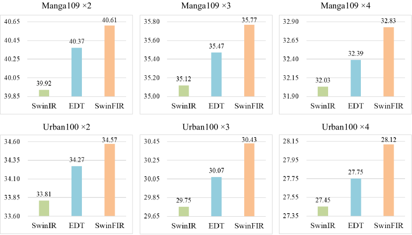
Figure 1: The comparison results of our SwinFIR with the state-of-the-art methods SwinIR and EDT. Under different scales ($\times 2,\times 3,\times 4$), our SwinFIR achieves the best performance than existing works.

The Vision Transformer (VIT) [13, 2, 41, 17, 30] has achieved great success in the high-level vision task. Therefore, Liang et al. [28] explore the potential of VIT in the low-level vision tasks and propose SwinIR. SwinIR, which is based on Swin Transformer [30], outperforms the state-of-the-art methods on image restoration tasks such as image super-resolution, and image denoising. It consists of three components: shallow feature extraction, deep feature extraction and high-quality image reconstruction. The fundamental unit of deep feature extraction is called RSTB (Residual Swin Transformer Block), and each RSTB is made up of many Swin Transformer layers and residual connections. In detail, the RSTB performs the self-attention in each window and uses Shift Window strategy to expand the receptive field. However, this limited shift cannot effectively perceive the global information in the early layers.

Global information is essential for image super-resolution (SR) since it can activate more pixels and is beneficial to improve the image reconstruction performance [16]. Therefore, in order to utilize global information, we revisit the SwinIR architecture and introduce a new model specifically designed for SR task, called SwinFIR. The Spatial Frequency Block (SFB), which is based on Fast Fourier Convolution (FFC) [5] and substitutes the convolution layer of the deep feature extraction module of SwinIR, is the essential innovation for SwinFIR. SFB consists of two branches: spatial and frequency model. We employ the FFC to extract the global information in the frequency branch and the CNN-based residual module in the spatial branch to enhance local feature expression.

In addition to the SFB module, we also revisit a variety of methods to improve the image super-resolution performance, such as data augmentation, loss function, pre-training strategy, post-processing, etc. Data Augmentation (DA) based on the pixel-domain, which is extensively used and has yielded impressive results in high-level tasks, is rarely studied in SR (super-resolution) tasks. A lot of works [10, 18, 43, 44] have proved that effective DA can inhibit overfitting and improve the generalization ability of the model. Therefore, we believe that exploring effective DA will certainly boost the effectiveness of image super-resolution. And we demonstrate through experiments that efficient data augmentation approaches, such as channel shuffle and Mixup, can considerably enhance the performance of image super-resolution. At the same time, we propose a brand-new feature-ensemble post-processing technique that is inspired by self-ensemble. The feature ensemble method enables the performance of the model to be considerably enhanced without increasing the training and testing time.

The comparison results of our SwinFIR with the state-of-the-art methods SwinIR [28] and EDT [26] on Manga109 and Urban100 datasets as shown in Figure 1. Experimental results demonstrate that these strategies can effectively improve the performance of image super-resolution and our SwinFIR achieves state-of-the-art (SOTA) performance on all benchmarks. Specifically, our SwinFIR is 0.30 $\sim$ 0.80 dB and 0.24 $\sim$ 0.44 dB higher than the SOTA methods of SwinIR and EDT on the Manga109 and the Urban100 dataset, respectively, by using these strategies.

Our contributions can be summarized as follows:

• We revisit the SwinIR architecture and introduce the Spatial Frequency Block (SFB) specifically designed for utilizing global information in SR task, called SwinFIR. SFB is based on Fast Fourier Convolution (FFC) and used extract more comprehensive, detailed, and stable features. SFB consists of two branches: spatial and frequency model. We employ the FFC to extract the global information in the frequency branch and the residual module in the spatial branch to enhance local feature expression.

• We revisit various data augmentation methods in low-level tasks and demonstrate that efficient data augmentation approaches, such as channel shuffle and mixup, can considerably boost the performance of image super-resolution. Our method breaks the inertial thinking that data enhancement methods such as inserting new pixels will affect SR performance.

• We propose a brand-new ensemble strategy called feature ensemble, which integrates multiple trained models to get a better and more comprehensive model without increasing training and testing time, and is a zero-cost method to improve performance.

2 Related Works

Image Super Resolution (SR) is defined as the process of restoring a High Resolution (HR) image from a Low Resolution (LR) image. In recent years, SR models have been actively explored and achieved state-of-the-art performance with the rapid development of deep learning technology. SRCNN [11] is the pioneering work of deep learning in SR. The network structure is very simple and only three convolutional layers are used. EDSR [29] improves performance by removing unnecessary modules in residual networks and expanding the model size. RCAN [45] proposes the Channel Attention mechanism to adaptively rescale features of each channel by modeling the interdependencies between feature channels. HAN [33] further explores the application of attention mechanisms in SR task by modeling the interdependencies between different layers, different channels and different locations. Although all of these CNN-based works achieves excellent performance in SR tasks, CNN suffers from the limitations of the receptive field, and Transformer starts to be acting outstandingly in SR tasks due to its superior remote modeling capability.

IPT [3] is a pre-trained Transformer model on the low-level visual task that introduces the Transformer module in the feature map processing stage. HAT [4] is a Hybrid Attention Transformer that combines multiple attention mechanisms, such as channel attention, self-attention, and overlapping cross-attention. SwinIR [28] is an image restoration model based on Swin Transformer. However, the potential of the Transformer still cannot be fully exploited by existing work, and our method adapts the SwinIR-based network architecture by introducing the SFB module based on FFC [5] that can activate more input information. LaMa [36] proposes a new image restoration network based on FFC. Inspired by LaMa, we propose the SFB, which employs large receptive field operations within early layers of the network, and can take advantage of long dependencies to use more pixels for better performance.

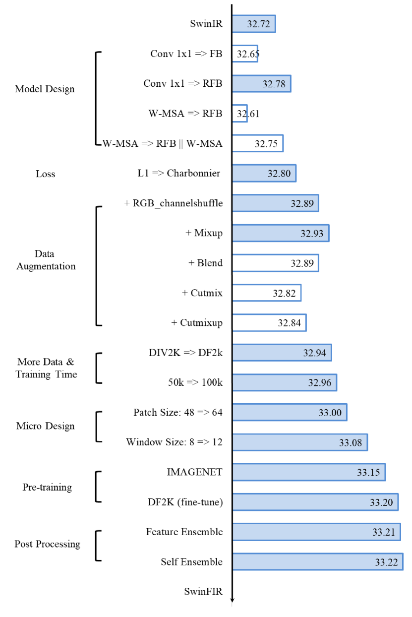
Figure 2: The evolution trajectory from SwinIR to SwinFIR. All models are evaluated on Set5 ($\times$4) dataset.

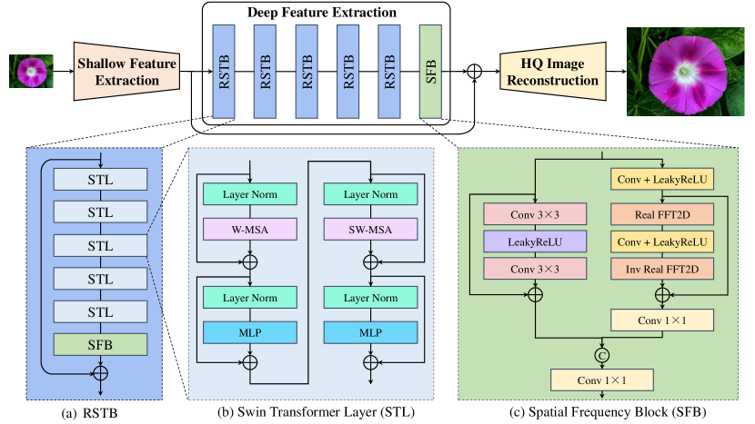
Figure 3: The network architecture of SwinFIR.

3 Methodology

In this paper, we revisit the strategies for improving image super-resolution, that involve little or no additional model parameters and calculations. The evolution trajectory from SwinIR to SwinFIR is shown in Figure 2. LAM [16] demonstrate that global information is essential for image super-resolution (SR) since it can activate more pixels and is beneficial to improve the image reconstruction performance. Consequently, we first revisit the SwinIR architecture and introduce the Spatial Frequency Block (SFB) specifically designed for utilizing global information in SR tasks. Then we replace L1 Loss with a more stable Charbonnier Loss [23]. We also revisit a number of data augmentation techniques that can enhance the effectiveness of image super-resolution. Loss function and data augmentation strategy are the training and testing free methods. We also examine various popular methods for enhancing image super-resolution performance, such as using more training data, enlarging the window size of Swin Transformer and employing pre-training model. Finally, inspired by self-ensemble, we propose a novel post-processing technique, named feature ensemble, to improve the stability of the model without lengthening the training and testing periods. All models are evaluated on Set5 ($\times$4) dataset in Figure 2.

3.1 Model Design

Inspired by SwinIR, we propose SwinFIR using Swin Transformer and Fast Fourier Convolution, as shown in Figure 3. SwinFIR consists of three modules: shallow feature extraction, deep feature extraction and high-quality (HQ) image reconstruction modules. The shallow feature extraction and high-quality (HQ) image reconstruction modules adopt the same configuration as SwinIR. The residual Swin Transformer block (RSTB) is a residual block with Swin Transformer layers (STL) and convolutional layers in SwinIR. They all have local receptive fields and cannot extract the global information of the input image. The Fast Fourier Convolution has the ability to extract global features, so we replace the convolution (3$\times$3) with Fast Fourier Convolution and a residual module to fuse global and local features, named Spatial Frequency Block (SFB), to improve the representation ability of model. The analysis of Frequency Block (FB), Spatial-Frequency Transformer Layer (SFTL) and Hybrid Swin Transformer Layer (HSTL) are in Figure 4 and sec. 4.4.1.

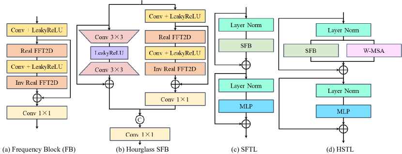
Figure 4: (a) Frequency Block (FB), (b) Hourglass Spatial Frequency Block (Hourglass SFB), (c) Spatial-Frequency Transformer Layer (SFTL) and (d) Hybrid Swin Transformer Layer (HSTL). The detail information in the sec. 4.4.1.

The SFB network architecture is shown in Figure 3(c) and is composed of two primary components: a spatial conventional convolution operation on the left and a Fast Fourier convolution (FFC) on the right. We concatenate the left and right outputs, and perform a convolution operation to obtain the final result. The formula is as follows,

$$X_{SFB}=H_{SFB}(X)$$ (1)

where the $X$ is the feature map from STL. $H_{SFB}(\cdot)$ represents the SFB module and $X_{SFB}$ is the output feature map after various operations of SFB. We send $X$ into two distinct domains, $X_{spatial}$ and $X_{frequency}$. $X_{spatial}$ is utilized in the spatial domain, and $X_{frequency}$ is intended to capture the long-range context in the frequency domain,

$$X_{spatial}=H_{spatial}(X)$$ (2)

$$X_{frequency}=H_{frequency}(X)$$ (3)

where $H_{spatial}(\cdot)$ is the spatial convolution module and $H_{frequency}(\cdot)$ represents the frequency FFC module. The left spatial convolution module is a residual module for classical SR and a hourglass residual module for lightweight SR, as shown in 3(c) and 4(b) respectively. Compared to a single-layer convolution, we insert a residual connection and convolution layer to increase the expressiveness of the model. Experiments have shown that this simple modification increases performance dramatically. The $X_{spatial}$ is also represented as,

$$X_{spatial}=H_{CLC}(X)+X$$ (4)

where $H_{CLC}(\cdot)$ denotes a 3$\times$3 convolution layer at the head and tail, and LeakyReLU operation is conducted between convolution layers. In the right frequency module, we transform the conventional spatial features into the frequency domain to extract the global information by using the 2-D Fast Fourier Transform (FFT). And we then perform inverse 2-D FFT operation to obtain spatial domain features. The $X_{frequency}$ is also represented as,

$$X=H_{CL}(X)$$ (5)

$$X_{frequency}=H_{C}(H_{FLF}(X)+X)$$ (6)

where $H_{CL}(\cdot)$ denotes a convolution layer and LeakyReLU. $H_{FLF}(\cdot)$ contains the following series of operations, a 2-D FFT based on a channel-wise, a compilation operation with frequency convolution and LeakeyReLU and an inverse 2-D FFT operation. The number of channels is then reduced in half by a convolution operation,

$$X_{SFB}=H_{C}([X_{spatial}||X_{frequency}])$$ (7)

where $H_{C}(\cdot)$ denotes a convolution layer and $||$ stands for the concatenation operator.

3.2 Loss Function

In addition to the structure of the neural network, the loss function also determines whether the model can achieve good results. In low-level visual tasks, such as super resolution and deblurring, the $L2$ [12], $L1$ [45], perceptual and adversarial [34] loss functions are often used to optimize neural networks. However, we use Charbonnier loss function [23] to optimize our SwinFIR to get better performance than other loss functions. In the training phase, the loss function is minimized by training data $\{I_{L}^{i},I_{H}^{i}\}_{i=1}^{N}$ to update the parameters, $N$ represent the numbers of training images. The Charbonnier loss function is,

$$L(\theta)=\frac{1}{N}\sum_{i=1}^{N}\sqrt{(SwinFIR(I_{L}^{i},\theta)-I_{H}^{i})^{2}+\varepsilon}$$ (8)

where $\theta$ denotes the parameters of SwinFIR.

3.3 Data Augmentation

Radu et al. propose rotation and flip data enhancement approaches based on spatial transformation, which is widely used at low-level tasks. However, data augmentation based on the pixel-domain, which is extensively used and has yielded impressive results in high-level tasks, is rarely studied in low-level tasks. In this paper, in addition to flip and rotation, we revisit the effect of data augmentations based on the pixel-domain on image super-resolution, such as RGB channel shuffle, Mixup, Blend, CutMix and CutMixup. RGB channel shuffle randomly shuffles the RGB channels of input images for color augmentation. Mixup randomly mixes the two images according to a certain proportion. Blend randomly adds fixed pixel to input images. CutMix and CutMixup are the combination of Mixup and Cutout. We illustrate in Figure 2 how various data augmentations affect the performance of image super-resolution on the Set5 dataset. All techniques, except CutMix and CutMixup which destroy visual continuity, are used for data augmentation and achieved performance gains.

Using more training data, enlarging the window size of Swin Transformer and employing pre-training model have all been demonstrated to be feasible in previous studies, so we won’t discuss these here.

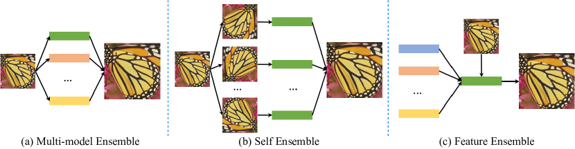
Figure 5: (a) Multi-model Ensemble, (b) Self Ensemble and (c) Feature Ensemble. Rectangles with different colors represent different model parameters.

3.4 Feature Ensemble

From the beginning of training the model to the convergence, there will be many intermediate models. In general, the model with the highest performance on the validation set will be selected as the final one, and other models will be deleted. Multi-model ensemble and self-ensembles are often used to improve the performance of SR, as shown in Figure 5. Multi-model ensemble combines the inference results from various models. Self-ensemble averages the transformed outputs from one model and input image. They have the same drawback, that is, they will multiply the inference time. We propose a novel ensemble strategy without lengthening the training and testing periods. Specifically, we select multiple models that performed well on the validation dataset and combine them using the weighted average method. Our feature ensemble strategy can steadily improve the performance of the model and can be applied to any task, including low-level and high-level.

$$SwinFIR(\theta)=\sum_{i=1}^{n}{SwinFIR(\theta)^{i}*\alpha^{i}}$$ (9)

where $\theta$ denotes the parameter sets of SwinFIR, $n$ is the numbers of models. $\alpha$ is the weight of each model and the $\alpha=\frac{1}{n}$ in this paper.

4 Experiments

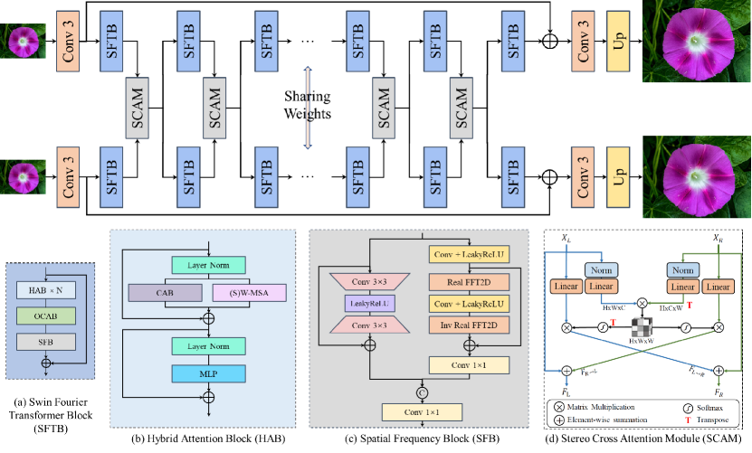
Figure 6: The network architecture of our SwinFIRSSR for stereo image super-resolution.

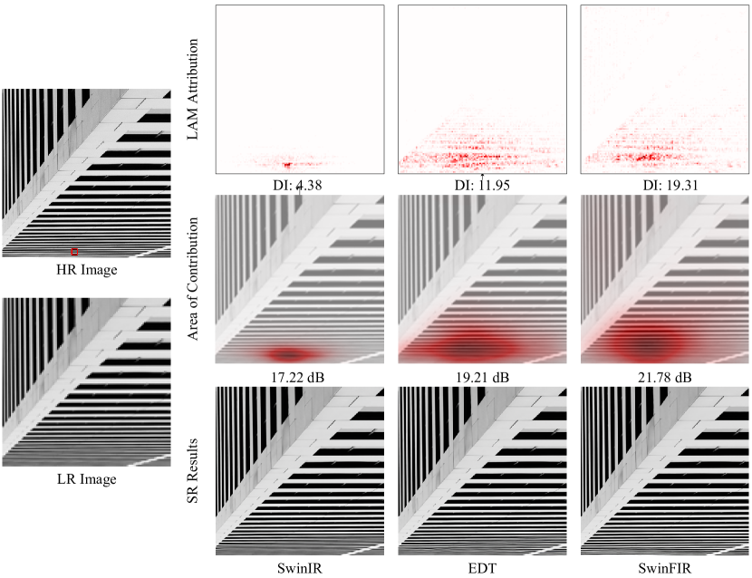
Figure 7: LAM comparisons between SwinIR and EDT on Urban100($\times 4$) img_011. The results indicate that SwinFIR utilize more information than SwinIR and EDT.

Method	Scale	Training Dataset	Set5		Set14		BSD100		Urban100		Manga109
			PSNR	SSIM	PSNR	SSIM	PSNR	SSIM	PSNR	SSIM	PSNR	SSIM
EDSR	$\times$2	DIV2K	38.11	0.9602	33.92	0.9195	32.32	0.9013	32.93	0.9351	39.10	0.9773
RCAN	$\times$2	DIV2K	38.27	0.9614	34.12	0.9216	32.41	0.9027	33.34	0.9384	39.44	0.9786
SAN	$\times$2	DIV2K	38.31	0.9620	34.07	0.9213	32.42	0.9028	33.10	0.9370	39.32	0.9792
IGNN	$\times$2	DIV2K	38.24	0.9613	34.07	0.9217	32.41	0.9025	33.23	0.9383	39.35	0.9786
HAN	$\times$2	DIV2K	38.27	0.9614	34.16	0.9217	32.41	0.9027	33.35	0.9385	39.46	0.9785
NLSN	$\times$2	DIV2K	38.34	0.9618	34.08	0.9231	32.43	0.9027	33.42	0.9394	39.59	0.9789
SwinIR	$\times$2	DF2K	38.42	0.9623	34.46	0.9250	32.53	0.9041	33.81	0.9427	39.92	0.9797
EDT	$\times$2	DF2K	38.45	0.9624	34.57	0.9258	32.52	0.9041	33.80	0.9425	39.93	0.9800
SwinFIR (Ours)	$\times$2	DF2K	38.57	0.9630	34.66	0.9263	32.59	0.9049	34.30	0.9459	40.30	0.9809
IPT†	$\times$2	ImageNet	38.37	-	34.43	-	32.48	-	33.76	-	-	-
EDT†	$\times$2	DF2K	38.63	0.9632	34.80	0.9273	32.62	0.9052	34.27	0.9456	40.37	0.9811
SwinFIR† (Ours)	$\times$2	DF2K	38.65	0.9633	34.93	0.9276	32.64	0.9054	34.57	0.9473	40.61	0.9816
EDSR	$\times$3	DIV2K	34.65	0.9280	30.52	0.8462	29.25	0.8093	28.80	0.8653	34.17	0.9476
RCAN	$\times$3	DIV2K	34.74	0.9299	30.65	0.8482	29.32	0.8111	29.09	0.8702	34.44	0.9499
SAN	$\times$3	DIV2K	34.75	0.9300	30.59	0.8476	29.33	0.8112	28.93	0.8671	34.30	0.9494
IGNN	$\times$3	DIV2K	34.72	0.9298	30.66	0.8484	29.31	0.8105	29.03	0.8696	34.39	0.9496
HAN	$\times$3	DIV2K	34.75	0.9299	30.67	0.8483	29.32	0.8110	29.10	0.8705	34.48	0.9500
NLSN	$\times$3	DIV2K	34.85	0.9306	30.70	0.8485	29.34	0.8117	29.25	0.8726	34.57	0.9508
SwinIR	$\times$3	DF2K	34.97	0.9318	30.93	0.8534	29.46	0.8145	29.75	0.8826	35.12	0.9537
EDT	$\times$3	DF2K	34.97	0.9316	30.89	0.8527	29.44	0.8142	29.72	0.8814	35.13	0.9534
SwinFIR (Ours)	$\times$3	DF2K	35.13	0.9328	31.13	0.8556	29.52	0.8161	30.20	0.8885	35.53	0.9554
IPT†	$\times$3	ImageNet	34.81	-	30.85	-	29.38	-	29.49	-	-	-
EDT†	$\times$3	DF2K	35.13	0.9328	31.09	0.8553	29.53	0.8165	30.07	0.8863	35.47	0.9550
SwinFIR† (Ours)	$\times$3	DF2K	35.15	0.9330	31.24	0.8566	29.55	0.8169	30.43	0.8913	35.77	0.9563
EDSR	$\times$4	DIV2K	32.46	0.8968	28.80	0.7876	27.71	0.7420	26.64	0.8033	31.02	0.9148
RCAN	$\times$4	DIV2K	32.63	0.9002	28.87	0.7889	27.77	0.7436	26.82	0.8087	31.22	0.9173
SAN	$\times$4	DIV2K	32.64	0.9003	28.92	0.7888	27.78	0.7436	26.79	0.8068	31.18	0.9169
IGNN	$\times$4	DIV2K	32.57	0.8998	28.85	0.7891	27.77	0.7434	26.84	0.8090	31.28	0.9182
HAN	$\times$4	DIV2K	32.64	0.9002	28.90	0.7890	27.80	0.7442	26.85	0.8094	31.42	0.9177
NLSN	$\times$4	DIV2K	32.59	0.9000	28.87	0.7891	27.78	0.7444	26.96	0.8109	31.27	0.9184
SwinIR	$\times$4	DF2K	32.92	0.9044	29.09	0.7950	27.92	0.7489	27.45	0.8254	32.03	0.9260
EDT	$\times$4	DF2K	32.82	0.9031	29.09	0.7939	27.91	0.7483	27.46	0.8246	32.05	0.9254
SwinFIR (Ours)	$\times$4	DF2K	33.08	0.9048	29.21	0.7971	27.98	0.7508	27.87	0.9348	32.52	0.9292
IPT†	$\times$4	ImageNet	32.64	-	29.01	-	27.82	-	27.26	-	-	-
EDT†	$\times$4	DF2K	33.06	0.9055	29.23	0.7971	27.99	0.7510	27.75	0.8317	32.39	0.9283
SwinFIR† (Ours)	$\times$4	DF2K	33.20	0.9068	29.36	0.7993	28.03	0.7520	28.12	0.8393	32.83	0.9314

Table 1: Quantitative comparison with state-of-the-art methods on benchmark datasets on the Y channel from the YCbCr space for classical image SR. The top two results are marked in red and blue. “$\dagger$” indicates that methods adopt pre-training strategy on ImageNet.

Urban100($\times$4): img_004 EDSR IGNN HAN IPT RNAN RCAN SwinIR EDT SwinFIR(ours) Reference

Urban100($\times$4): img_044 EDSR IGNN HAN IPT RNAN RCAN SwinIR EDT SwinFIR(ours) Reference

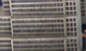
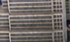
Urban100($\times$4): img_073 EDSR IGNN HAN IPT RNAN RCAN SwinIR EDT SwinFIR(ours) Reference

Figure 8: Visual results ($\times$4) achieved by different methods on the Urban100 dataset (classical image SR).

4.1 Datasets

Following EDT [26], we pre-train the SwinFIR on ImageNet 2012 [9]. The SwinFIR is then fine-tuned for Classical and Lightweight SR using sub-images (384$\times$384) that were generated by cropping the high-resolution DF2K (DIV2K [29] + Flicker2K [38]) dataset. We perform validation on Image Super-Resolution benchmark datasets Set5, Set14, BSD100, Urban100 and Manga109 for Classical and Lightweight SR. We perform data augmentation on training data to improve the robustness of SwinFIR, which includes horizontal flip, vertical flip, rotation, channel shuffle and Mixup.

4.2 Implementation Details

We revisit the long-dependent modeling capabilities of SwinIR and propose an efficient global feature extractor based on Fast Fourier Convolution (FFC). Specifically, we replace the convolution layer in RSTB of SwinIR with Spatial Frequency Block (SFB). For classical image SR, we utilize the same configuration as SwinIR. We also investigate how performance of SR is affected by large window and patch size. As a result, we use a larger window size 12 and patch size 60 in our work. For lightweight image SR, we also decrease RSTB number and channel number to 4 and 60 follow SwinIR, respectively. However, we use 5 STL in the second and third RSTB to accelerate training and inference time.

We extend the SwinFIR to SwinFIRSSR following NAFSSR [6] and HAT [4], and verify the effectiveness of our method in the stereo image super-resolution task, as shown in Figure. 6. HAT proposed the Residual Hybrid Attention Group (RHAG) to activating more pixel in image super-resolution transformer for improve the performance. RHAG contains N hybrid attention blocks (HAB), an overlapping cross-attention block (OCAB) and a 3$\times$3 convolutional layer, we replace the convolution (3$\times$3) with Fast Fourier Convolution and a residual module to fuse global and local features, named Spatial-frequency Block (SFB), to improve the representation ability of model. We also follow the NAFSSR to attend and fuse the left/right viewpoint features by using stereo cross-attention module (SCAM).

We use the Adam with $\beta_{1}=0.9$ and $\beta_{2}=0.99$ and weight decay 0 by default to optimize the Charbonnier loss function for classical image SR and lightweight image SR. In the pre-training stage, the initial learning rate is 2e-4 and reduces by 50% in 500,000, 800,000, 900,000, and 950,000 iterations for a total of 1,000,000 iterations, respectively. In the fine-tune stage, the learning rate is decreased to 1e-5 for classical and lightweight image SR.

4.3 Comparison to state-of-the-arts methods

4.3.1 Classical Image Super-Resolution

Modern algorithms such as EDSR [29], RCAN [45], SAN [8], IGNN [48], RNAN [46], HAN [33], NLSA [31], IPT [3], SwinIR [28], and EDT [26] are compared to our SwinFIR. The DIV2K dataset was used to train the CNN-based methods EDSR, RCAN, SAN, IGNN, RNAN, HAN, and NLSA. Networks based on Vision Transformer include IPT, SwinIR, and EDT. IPT and EDT are trained on the ImageNet dataset, while EDT is fine-tuned on the DF2K dataset to get better performance. And SwinIR only is trained on the DF2K dataset. Following EDT, our SwinFIR is first trained on the ImageNet, and then fine-tuned on the DF2K dataset. Table 1 displays the quantitative results on benchmark datasets for classical SR. Our SwinFIR achieves the best SR performance on $\times$2, $\times$3 and $\times$4 scales compared with other state-of-the-art methods. Especially, SwinFIR improves the PSNR of SwinIR from 27.45 dB and 32.03 dB to 28.12 dB and 32.83 dB on $\times$4 scales of Urban100 and Manga109 datasets respectively, 0.77 dB and 0.80 dB higher than its. It demonstrates the effectiveness of our proposed method and represents a major improvement over the image super-resolution task. Even without pre-training, our SwinFIR achieves better or comparable performance than EDT with pre-training, 0.13 dB higher on $\times$4 scales of Manga109 datasets.

Visual results are shown in Figure 8, and the images restored by our SwinFIR are clearer. Our SwinFIR can restore high-frequency details based on Fast Fourier Convolution (FFC). Especially, Our SwinFIR performs better when trying to restore images with periodic transformations. It is worth mentioning that the current approaches, whether based on CNN or Transformer, are inadequate for challenging samples, as shown in Figure 8. And our method addresses this issue by making slight adjustments to the SwinIR, which can significantly improve performance.

The LAM results are shown in Figure 7. The LAM attribution map and area of contribution accurately depict the significance of each pixel and receptive field size in the input LR image when reconstructing the red box region of the SR images. The Diffusion Index (DI) illustrates the range of relevant and utilised pixels. The higher the DI, the wider range of pixels are used. Furthermore, SwinFIR outperforms SwinIR and EDT in terms of DI, as shown in Figure 7. And almost all of the pixels from the input LR image are used to restore the SR image in SwinFIR, according to the LAM attribution map. The qualitative and quantitative results demonstrate that SwinIR does has a limited receptive field, and our SwinFIR based FFC takes advantage of long dependencies to use more pixels for better performance.

4.3.2 Lightweight Image Super-Resolution

We substitute the Hourglass SFB for SFB in lightweight SwinFIR, named SwinFIR-T. And we compare SwinFIR-T with the SOTA lightweight SR methods, including SRCNN  [11], LapSRN [22], DRRN [37], CARN-M [1], SRFBN-S [27], IMDN [19], SwinIR (small size) and EDT-T. SwinFIR significantly improves image SR performance and achieves the best results for all metrics, as indicated by the quantitative comparison in Table 2. SwinFIR achieves 31.50dB PSNR on the Manga109 dataset ($\times$4) when the number of parameters are comparable to the SwinIR and EDT-T, which is 0.58 dB and 0.15 dB higher than them, respectively. In particular, SwinFIR achieves better or comparable performance to EDT when using a smaller window size. Visual results are presented in Figure 9, and the images restored by our SwinFIR are sharper and contain more high-frequency detail information. EDT and our SwinFIR all can recover the detailed information of the book on Set14 barbara dataset, but the reconstruction results of EDT are more blurring.

Scale	Method	#Param.	Flops	Set5		Set14		BSDS100		Urban100		Manga109
		(K)	(G)	PSNR	SSIM	PSNR	SSIM	PSNR	SSIM	PSNR	SSIM	PSNR	SSIM
$\times 2$	LAPAR	548	171.5	38.01	0.9605	33.62	0.9183	32.19	0.8999	32.10	0.9283	38.67	0.9772
	LatticeNet	756	171.2	38.15	0.9610	33.78	0.9193	32.25	0.9005	32.43	0.9302	-	-
	SwinIR	878	205.5	38.14	0.9611	33.86	0.9206	32.31	0.9012	32.76	0.9340	39.12	0.9783
	EDT-T	917	224.2	38.23	0.9615	33.99	0.9209	32.37	0.9021	32.98	0.9362	39.45	0.9789
	SwinFIR-T(Ours)	872	206.3	38.26	0.9616	34.08	0.9221	32.38	0.9024	33.14	0.9374	39.55	0.9790
$\times 3$	LAPAR	594	114.44	34.36	0.9267	30.34	0.8421	29.11	0.8054	28.15	0.8523	33.51	0.9441
	LatticeNet	765	77.0	34.53	0.9281	30.39	0.8424	29.15	0.8059	28.33	0.8538	-	-
	SwinIR	886	93.2	34.62	0.9289	30.54	0.8463	29.20	0.8082	28.66	0.8624	33.98	0.9478
	EDT-T	919	103.0	34.73	0.9299	30.66	0.8481	29.29	0.8103	28.89	0.8674	34.44	0.9498
	SwinFIR-T(Ours)	880	94.0	34.75	0.9300	30.68	0.8489	29.30	0.8106	29.04	0.8697	34.60	0.9506
$\times 4$	LAPAR	659	94..8	32.15	0.8944	28.61	0.7818	27.61	0.7366	26.14	0.7871	30.42	0.9074
	LatticeNet	777	44.2	32.30	0.8962	28.68	0.7830	27.62	0.7367	26.25	0.7873	-	-
	SwinIR	897	53.2	32.44	0.8976	28.77	0.7858	27.69	0.7406	26.47	0.7980	30.92	0.9151
	EDT-T	922	58.5	32.53	0.8991	28.88	0.7882	27.76	0.7433	26.71	0.8051	31.35	0.9180
	SwinFIR-T(Ours)	891	54.4	32.62	0.9002	28.95	0.7898	27.79	0.7440	26.85	0.8088	31.50	0.9199

Table 2: Quantitative comparison with state-of-the-art methods on benchmark datasets on the Y channel from the YCbCr space for lightweight image SR. The top two results are marked in red and blue.

Set14($\times$4): barbara SRCNN LapSRN DRRN CARN-M SRFBN-S IMDN SwinIR EDT SwinFIR(ours) Reference

Urban100($\times$4): img_092 SRCNN LapSRN DRRN CARN-M SRFBN-S IMDN SwinIR EDT SwinFIR(ours) Reference

Figure 9: Visual results ($\times$4) achieved by different methods on the Urban100 dataset (lightweight image SR).

img_0035 (Left) Bicubic StereoSR EDSR RCAN SRRes+SAM iPASSR SSRDE-FNet NAFSSR-L SwinFIRSSR(ours) Reference

img_0035 (Right) Bicubic StereoSR EDSR RCAN SRRes+SAM iPASSR SSRDE-FNet NAFSSR-L SwinFIRSSR(ours) Reference

Figure 10: Visual results ($\times$4) achieved by different methods on the Flickr1024 dataset (stereo image SR).

Method	Scale	$\#P$	Left			$\left(\textit{Left}+\textit{Right}\right)/2$
			KITTI 2012	KITTI 2015	Middlebury	KITTI 2012	KITTI 2015	Middlebury	Flickr1024
VDSR	$\times$2	0.66M	30.17$/$0.9062	28.99$/$0.9038	32.66$/$0.9101	30.30$/$0.9089	29.78$/$0.9150	32.77$/$0.9102	25.60$/$0.8534
EDSR	$\times$2	38.6M	30.83$/$0.9199	29.94$/$0.9231	34.84$/$0.9489	30.96$/$0.9228	30.73$/$0.9335	34.95$/$0.9492	28.66$/$0.9087
RDN	$\times$2	22.0M	30.81$/$0.9197	29.91$/$0.9224	34.85$/$0.9488	30.94$/$0.9227	30.70$/$0.9330	34.94$/$0.9491	28.64$/$0.9084
RCAN	$\times$2	15.3M	30.88$/$0.9202	29.97$/$0.9231	34.80$/$0.9482	31.02$/$0.9232	30.77$/$0.9336	34.90$/$0.9486	28.63$/$0.9082
StereoSR	$\times$2	1.08M	29.42$/$0.9040	28.53$/$0.9038	33.15$/$0.9343	29.51$/$0.9073	29.33$/$0.9168	33.23$/$0.9348	25.96$/$0.8599
PASSRnet	$\times$2	1.37M	30.68$/$0.9159	29.81$/$0.9191	34.13$/$0.9421	30.81$/$0.9190	30.60$/$0.9300	34.23$/$0.9422	28.38$/$0.9038
IMSSRnet	$\times$2	6.84M	30.90$/$-	29.97$/$-	34.66$/$-	30.92$/$-	30.66$/$-	34.67$/$-	-$/$-
iPASSR	$\times$2	1.37M	30.97$/$0.9210	30.01$/$0.9234	34.41$/$0.9454	31.11$/$0.9240	30.81$/$0.9340	34.51$/$0.9454	28.60$/$0.9097
SSRDE-FNet	$\times$2	2.10M	31.08$/$0.9224	30.10$/$0.9245	35.02$/$0.9508	31.23$/$0.9254	30.90$/$0.9352	35.09$/$0.9511	28.85$/$0.9132
NAFSSR-T	$\times$2	0.45M	31.12$/$0.9224	30.19$/$0.9253	34.93$/$0.9495	31.26$/$0.9254	30.99$/$0.9355	35.01$/$0.9495	28.94$/$0.9128
NAFSSR-S	$\times$2	1.54M	31.23$/$0.9236	30.28$/$0.9266	35.23$/$0.9515	31.38$/$0.9266	31.08$/$0.9367	35.30$/$0.9514	29.19$/$0.9160
NAFSSR-B	$\times$2	6.77M	31.40$/$0.9254	30.42$/$0.9282	35.62$/$0.9545	31.55$/$0.9283	31.22$/$0.9380	35.68$/$0.9544	29.54$/$0.9204
NAFSSR-L	$\times$2	23.79M	31.45$/$0.9261	30.46$/$0.9289	35.83$/$0.9559	31.60$/$0.9291	31.25$/$0.9386	35.88$/$0.9557	29.68$/$0.9221
SwinFIRSSR (Ours)	$\times$2	23.94M	31.65$/$0.9293	30.66$/$0.9321	36.48$/$0.9601	31.79$/$0.9321	31.45$/$0.9413	36.52$/$0.9598	30.14$/$0.9286
VDSR	$\times$4	0.66M	25.54$/$0.7662	24.68$/$0.7456	27.60$/$0.7933	25.60$/$0.7722	25.32$/$0.7703	27.69$/$0.7941	22.46$/$0.6718
EDSR	$\times$4	38.9M	26.26$/$0.7954	25.38$/$0.7811	29.15$/$0.8383	26.35$/$0.8015	26.04$/$0.8039	29.23$/$0.8397	23.46$/$0.7285
RDN	$\times$4	22.0M	26.23$/$0.7952	25.37$/$0.7813	29.15$/$0.8387	26.32$/$0.8014	26.04$/$0.8043	29.27$/$0.8404	23.47$/$0.7295
RCAN	$\times$4	15.4M	26.36$/$0.7968	25.53$/$0.7836	29.20$/$0.8381	26.44$/$0.8029	26.22$/$0.8068	29.30$/$0.8397	23.48$/$0.7286
StereoSR	$\times$4	1.42M	24.49$/$0.7502	23.67$/$0.7273	27.70$/$0.8036	24.53$/$0.7555	24.21$/$0.7511	27.64$/$0.8022	21.70$/$0.6460
PASSRnet	$\times$4	1.42M	26.26$/$0.7919	25.41$/$0.7772	28.61$/$0.8232	26.34$/$0.7981	26.08$/$0.8002	28.72$/$0.8236	23.31$/$0.7195
SRRes+SAM	$\times$4	1.73M	26.35$/$0.7957	25.55$/$0.7825	28.76$/$0.8287	26.44$/$0.8018	26.22$/$0.8054	28.83$/$0.8290	23.27$/$0.7233
IMSSRnet	$\times$4	6.89M	26.44$/$-	25.59$/$-	29.02$/$-	26.43$/$-	26.20$/$-	29.02$/$-	-$/$-
iPASSR	$\times$4	1.42M	26.47$/$0.7993	25.61$/$0.7850	29.07$/$0.8363	26.56$/$0.8053	26.32$/$0.8084	29.16$/$0.8367	23.44$/$0.7287
SSRDE-FNet	$\times$4	2.24M	26.61$/$0.8028	25.74$/$0.7884	29.29$/$0.8407	26.70$/$0.8082	26.43$/$0.8118	29.38$/$0.8411	23.59$/$0.7352
NAFSSR-T	$\times$4	0.46M	26.69$/$0.8045	25.90$/$0.7930	29.22$/$0.8403	26.79$/$0.8105	26.62$/$0.8159	29.32$/$0.8409	23.69$/$0.7384
NAFSSR-S	$\times$4	1.56M	26.84$/$0.8086	26.03$/$0.7978	29.62$/$0.8482	26.93$/$0.8145	26.76$/$0.8203	29.72$/$0.8490	23.88$/$0.7468
NAFSSR-B	$\times$4	6.80M	26.99$/$0.8121	26.17$/$0.8020	29.94$/$0.8561	27.08$/$0.8181	26.91$/$0.8245	30.04$/$0.8568	24.07$/$0.7551
NAFSSR-L	$\times$4	23.83M	27.04$/$0.8135	26.22$/$0.8034	30.11$/$0.8601	27.12$/$0.8194	26.96$/$0.8257	30.20$/$0.8605	24.17$/$0.7589
SwinFIRSSR (Ours)	$\times$4	24.09M	27.06$/$0.8175	26.15$/$0.8062	30.33$/$0.8676	27.16$/$0.8235	26.89$/$0.8283	30.44$/$0.8687	24.29$/$0.7681

Table 3: Quantitative results achieved by different methods on the KITTI 2012 [15], KITTI 2015 [32], Middlebury [35], and Flickr1024 [wang2019learning] datasets on the RGB space for stereo image SR. $\#P$ represents the number of parameters of the networks. Here, PSNR$/$SSIM values achieved on both the left images (i.e., Left) and a pair of stereo images (i.e., $\left(\textit{Left}+\textit{Right}\right)/2$) are reported.

4.3.3 Stereo Image Super-Resolution

We conduct a series of experiments in the stereo image SR and compare SwinFIRSSR to other SR methods. Single image SR methods include EDSR, RCAN, and RDN [47], whereas stereo image SR methods include StereoSR [20], PASSRnet [40], SRRes+SAM [42], IMSSRnet [25], iPASSR [24], SSRDE-FNet [7] and NAFSSR [6]. All models are trained on 800 Flickr1024 and 60 Middlebury images. Our SwinFIRSSR surpasses all single and stereo image SR methods, as shown in Table 3. When the number of parameters of our method is comparable to the SOTA method NAFSSR-L, our SwinFIRSSR performs better for $\times$2 stereo SR than NAFSSR-L by 0.19 dB, 0.20 dB, 0.64 dB and 0.46 dB on the KITTI2012 [15], KITTI2015 [32], Middlebury [35] and Flickr1024 testing dataset, respectively. The visual comparison results are shown in Figure 10. The SR images reconstructed by our SwinFIRSSR are clearer and offer a wealth of details and textures. The quantitative and qualitative results on stereo SR datasets demonstrate the effectiveness and robustness of our SwinFIRSSR.

4.4 Ablation Study

4.4.1 Impact of RFB

We try using the original FB, named Spectral Transform in [36], to replace the convolution module in the RSTB to extract global features from the low resolution image. However, this does not lead to the expected performance improvement for image SR, as shown in the Table 4. It can be seen intuitively from the LAM that local information has a higher contribution to image reconstruction. Therefore, we replace FB with SFB, that is, only adding a simple residual module to extract the local features of the input image can significantly improve the performance. At the same time, we also explore the influence of SFB position in RSTB on image reconstruction. We replace the attention module in STL with SFB and hybrid SFB to obtain SFTL and HSTL, as shown in the Figure 4. Although the performance of HSTL (37.20M) is better than that of SFB on Manga dataset, its parameters are 2.6 times that of SFB(14.03M), so we abandon this scheme.

	Method	Set5	Set14	BSD	Urban	Manga
Model Design	SwinIR	32.72	28.94	27.83	27.07	31.67
	FB	32.65	28.98	27.81	26.86	31.54
	SFB	32.78	29.01	27.86	27.11	31.69
Position	SFTL	32.61	28.89	27.78	26.91	31.49
	HSTL	32.75	28.98	27.85	27.07	31.76

Table 4: Impact of SFB with different model design and position.

4.4.2 Impact of Data Augmentations

Radu et al. propose seven ways of data augmentations methods without altered content. They contend that other data augmentations will introduce new pixels and degrade super-resolution performance. In addition to flip and rotation, we revisit the effect of data augmentations on image super-resolution. The channel shuffle and Mixup data augmentations improve the PSNR from 32.78 dB to 32.93 dB, which is 0.15 dB better than flip and rotation, as shown in Figure 2. The experiments demonstrate that the data augmentations methods based on inserting new pixels sometimes improve the performance of SR, breaking people’s previous cognition. However, not all data augmentations can improve image super-resolution performance. For example, CutMix and CutMixup boost the performance of image classification, but they have a drawback in the low-level tasks: they obliterate visual continuity. This drawback makes the image lose semantic information and reduces the available and useful information.

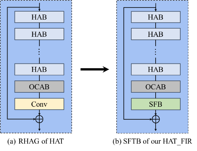
Figure 11: (a) Residual Hybrid Attention Group (RHAG) in the HAT. (b) Swin Fourier Transformer Block (SFTB) in our HAT_FIR. We replace the convolution (3$\times$3) in RHAG of HAT with SFB to get our SFTB.

Method	S	Set5	Set14	BSD	Urban	Manga
HAT	$\times$2	38.63	34.86	32.62	34.45	40.26
HAT_FIR (Ours)	$\times$2	38.63	34.63	32.62	34.47	40.39
+FE (Ours)	$\times$2	38.63	34.70	32.63	34.55	40.41
HAT†	$\times$2	38.73	35.13	32.69	34.81	40.71
HAT_FIR† (Ours)	$\times$2	38.74	35.16	32.71	34.92	40.72
+FE (Ours)	$\times$2	38.74	35.17	32.71	34.94	40.77
HAT	$\times$3	35.06	31.08	29.54	30.23	35.53
HAT_FIR (Ours)	$\times$3	35.13	31.15	29.54	30.40	35.60
+FE (Ours)	$\times$3	35.13	31.17	29.55	30.42	35.62
HAT†	$\times$3	35.16	31.33	29.59	30.70	35.84
HAT_FIR† (Ours)	$\times$3	35.20	31.36	29.60	30.74	35.90
+FE (Ours)	$\times$3	35.21	31.37	29.60	30.77	35.92
HAT	$\times$4	33.04	29.23	28.00	27.97	32.48
HAT_FIR (Ours)	$\times$4	33.09	29.23	28.01	28.13	32.64
+FE (Ours)	$\times$4	33.15	29.23	28.01	28.14	32.68
HAT†	$\times$4	33.18	29.38	28.05	28.37	32.87
HAT_FIR† (Ours)	$\times$4	33.26	29.44	28.07	28.40	33.02
+FE (Ours)	$\times$4	33.29	29.44	28.07	28.43	33.03

Table 5: Quantitative comparison with HAT.

Task	Method	S	DIV2K (val)	DIV2K (test)
SR	ABPN	$\times$3	30.14	29.87
	ABPN_FIR	$\times$3	30.18	29.95
	Method	$\sigma$	Set12	BSD68	Urban100
DN-G	SwinIR	15	33.36	31.97	33.70
	SwinFIR	15	33.42	32.00	33.85
	Method	$\sigma$	CBSD68	McMaster	Urban100
DN-C	SwinIR	15	34.42	35.61	35.13
	SwinFIR	15	34.43	35.64	35.34
	Method	$q$	Classic5
JPEG	SwinIR	10	30.27
	SwinFIR	10	30.65

Table 6: Quantitative comparison on different low-level tasks.

4.4.3 Robustness

HAT [4] propose a Hybrid Attention Transformer based on SwinIR and achieve the SOTA performance in image super-resolution task. So we also put HAT in our roadmap to verify the adaptability and robustness of our methods, as shown in Figure 11 and Table 5. Our training set and configuration are consistent with HAT in order to conduct a fair comparison. Our HAT_FIR improve the PSNR from 32.48 dB to 32.64 dB on Manga109 dataset ($\times 4$), which is 0.16 dB better than HAT. If we add the feature ensemble strategy into HAT_FIR, the performance will be further improved.

ABPN [14] is a simple but efficient image super-resolution method and wins the first place on Mobile AI 2021 Real-Time Image Super-Resolution Challenge (CVPR2021). We perform our method on ABPN without SFB to verify the robustness in the non-Transformer structure, as shown in Table 6. We improve the PSNR by 0.08 dB on DIV2K dataset without spending any additional time on inference. We also perform our SwinFIR on grayscale image denoising (DN-G), color image denoising (DN-C) and JPEG compression artifact reduction (JPEG) benchmark datasets. All experimental results demonstrate that our method can improve the image restoration performance on low-level tasks.

4.4.4 Impact of Feature Ensemble

SwinIR has indicated that post-processing methods such as self-ensemble can considerably improve the performance of image super-resolution. However, self-ensemble has a substantial disadvantage in that it takes longer to do inference. It is very unfriendly for the on-device side or time-sensitive scenarios. Inspired by self-ensemble, which ensembles the results of image super-resolution, we ensemble the parameters of the trained models , named feature ensemble. Experimental results demonstrate that our feature ensemble steadily improves the super-resolution performance with only once inference, as shown in the Table 5.

5 Conclusion

In this paper, we revisit how to improve the performance of image restoration. Firstly, we revisit the limitations of long-dependent modeling capabilities of SwinIR and propose an efficient global feature extractor based on Fast Fourier Convolution (FFC), named SwinFIR. Furthermore, we also revisit other strategies for improving SR performance, including data augmentation, loss function, pre-training, and feature ensemble. The results demonstrate that our SwinFIR has a wider receptive field than SwinIR, and takes advantage of long dependencies based on FFC to use more pixels for better performance. In particular, our feature ensemble strategy steadily improves performance without lengthening the training and testing periods. Extensive experiments on popular benchmarks demonstrate that our SwinFIR surpasses current models and our methods can significantly improve the performance of image restoration.

References

- [1] Namhyuk Ahn, Byungkon Kang, and Kyung Ah Sohn. Fast, accurate, and lightweight super-resolution with cascading residual network: 15th european conference, munich, germany, september 8-14, 2018, proceedings, part x. Springer, Cham, 2018.
- [2] Nicolas Carion, Francisco Massa, Gabriel Synnaeve, Nicolas Usunier, Alexander Kirillov, and Sergey Zagoruyko. End-to-end object detection with transformers. In European conference on computer vision, pages 213–229. Springer, 2020.
- [3] Hanting Chen, Yunhe Wang, Tianyu Guo, Chang Xu, Yiping Deng, Zhenhua Liu, Siwei Ma, Chunjing Xu, Chao Xu, and Wen Gao. Pre-trained image processing transformer. In Proceedings of the IEEE/CVF Conference on Computer Vision and Pattern Recognition, pages 12299–12310, 2021.
- [4] Xiangyu Chen, Xintao Wang, Jiantao Zhou, and Chao Dong. Activating more pixels in image super-resolution transformer. arXiv preprint arXiv:2205.04437, 2022.
- [5] Lu Chi, Borui Jiang, and Yadong Mu. Fast fourier convolution. Advances in Neural Information Processing Systems, 33:4479–4488, 2020.
- [6] Xiaojie Chu, Liangyu Chen, and Wenqing Yu. Nafssr: Stereo image super-resolution using nafnet. In Proceedings of the IEEE/CVF Conference on Computer Vision and Pattern Recognition (CVPR) Workshops, pages 1239–1248, June 2022.
- [7] Q. Dai, J. Li, Q. Yi, F. Fang, and G. Zhang. Feedback network for mutually boosted stereo image super-resolution and disparity estimation. 2021.
- [8] Tao Dai, Jianrui Cai, Yongbing Zhang, Shu-Tao Xia, and Lei Zhang. Second-order attention network for single image super-resolution. In Proceedings of the IEEE/CVF conference on computer vision and pattern recognition, pages 11065–11074, 2019.
- [9] Jia Deng, Wei Dong, Richard Socher, Li-Jia Li, Kai Li, and Li Fei-Fei. Imagenet: A large-scale hierarchical image database. In 2009 IEEE conference on computer vision and pattern recognition, pages 248–255. Ieee, 2009.
- [10] Terrance DeVries and Graham W Taylor. Improved regularization of convolutional neural networks with cutout. arXiv preprint arXiv:1708.04552, 2017.
- [11] Chao Dong, Chen Change Loy, Kaiming He, and Xiaoou Tang. Image super-resolution using deep convolutional networks. IEEE transactions on pattern analysis and machine intelligence, 38(2):295–307, 2015.
- [12] Chao Dong, Chen Change Loy, and Xiaoou Tang. Accelerating the super-resolution convolutional neural network. In European conference on computer vision, pages 391–407. Springer, 2016.
- [13] Alexey Dosovitskiy, Lucas Beyer, Alexander Kolesnikov, Dirk Weissenborn, Xiaohua Zhai, Thomas Unterthiner, Mostafa Dehghani, Matthias Minderer, Georg Heigold, Sylvain Gelly, et al. An image is worth 16x16 words: Transformers for image recognition at scale. arXiv preprint arXiv:2010.11929, 2020.
- [14] Zongcai Du, Jie Liu, Jie Tang, and Gangshan Wu. Anchor-based plain net for mobile image super-resolution. In Proceedings of the IEEE/CVF Conference on Computer Vision and Pattern Recognition, pages 2494–2502, 2021.
- [15] Andreas Geiger, Philip Lenz, and Raquel Urtasun. Are we ready for autonomous driving? the kitti vision benchmark suite. In 2012 IEEE conference on computer vision and pattern recognition, pages 3354–3361. IEEE, 2012.
- [16] Jinjin Gu and Chao Dong. Interpreting super-resolution networks with local attribution maps. In Proceedings of the IEEE/CVF Conference on Computer Vision and Pattern Recognition, pages 9199–9208, 2021.
- [17] Ruohao Guo, Dantong Niu, Liao Qu, and Zhenbo Li. Sotr: Segmenting objects with transformers. In Proceedings of the IEEE/CVF International Conference on Computer Vision, pages 7157–7166, 2021.
- [18] Dan Hendrycks and Thomas Dietterich. Benchmarking neural network robustness to common corruptions and perturbations. arXiv preprint arXiv:1903.12261, 2019.
- [19] Z. Hui, X. Gao, Y. Yang, and X. Wang. Lightweight image super-resolution with information multi-distillation network. ACM, 2019.
- [20] D. S. Jeon, S. H. Baek, I. Choi, and H. K. Min. Enhancing the spatial resolution of stereo images using a parallax prior. In 2018 IEEE/CVF Conference on Computer Vision and Pattern Recognition (CVPR), 2018.
- [21] Jiwon Kim, Jung Kwon Lee, and Kyoung Mu Lee. Deeply-recursive convolutional network for image super-resolution. In Proceedings of the IEEE conference on computer vision and pattern recognition, pages 1637–1645, 2016.
- [22] Wei-Sheng Lai, Jia-Bin Huang, Narendra Ahuja, and Ming-Hsuan Yang. Deep laplacian pyramid networks for fast and accurate super-resolution. In Proceedings of the IEEE conference on computer vision and pattern recognition, pages 624–632, 2017.
- [23] Wei-Sheng Lai, Jia-Bin Huang, Narendra Ahuja, and Ming-Hsuan Yang. Fast and accurate image super-resolution with deep laplacian pyramid networks. IEEE transactions on pattern analysis and machine intelligence, 41(11):2599–2613, 2018.
- [24] J. Lei, Z. Zhang, X. Fan, B. Yang, and Q. Huang. Deep stereoscopic image super-resolution via interaction module. IEEE Transactions on Circuits and Systems for Video Technology, PP(99):1–1, 2020.
- [25] Jianjun Lei, Zhe Zhang, Xiaoting Fan, Bolan Yang, Xinxin Li, Ying Chen, and Qingming Huang. Deep stereoscopic image super-resolution via interaction module. IEEE Transactions on Circuits and Systems for Video Technology, 31(8):3051–3061, 2020.
- [26] Wenbo Li, Xin Lu, Jiangbo Lu, Xiangyu Zhang, and Jiaya Jia. On efficient transformer and image pre-training for low-level vision. arXiv preprint arXiv:2112.10175, 2021.
- [27] Z. Li, J. Yang, Z. Liu, X. Yang, and W. Wu. Feedback network for image super-resolution. In 2019 IEEE/CVF Conference on Computer Vision and Pattern Recognition (CVPR), 2019.
- [28] Jingyun Liang, Jiezhang Cao, Guolei Sun, Kai Zhang, Luc Van Gool, and Radu Timofte. Swinir: Image restoration using swin transformer. In Proceedings of the IEEE/CVF International Conference on Computer Vision, pages 1833–1844, 2021.
- [29] Bee Lim, Sanghyun Son, Heewon Kim, Seungjun Nah, and Kyoung Mu Lee. Enhanced deep residual networks for single image super-resolution. In Proceedings of the IEEE conference on computer vision and pattern recognition workshops, pages 136–144, 2017.
- [30] Ze Liu, Yutong Lin, Yue Cao, Han Hu, Yixuan Wei, Zheng Zhang, Stephen Lin, and Baining Guo. Swin transformer: Hierarchical vision transformer using shifted windows. In Proceedings of the IEEE/CVF International Conference on Computer Vision, pages 10012–10022, 2021.
- [31] Yiqun Mei, Yuchen Fan, and Yuqian Zhou. Image super-resolution with non-local sparse attention. In Proceedings of the IEEE/CVF Conference on Computer Vision and Pattern Recognition, pages 3517–3526, 2021.
- [32] Moritz Menze and Andreas Geiger. Object scene flow for autonomous vehicles. In Proceedings of the IEEE conference on computer vision and pattern recognition, pages 3061–3070, 2015.
- [33] Ben Niu, Weilei Wen, Wenqi Ren, Xiangde Zhang, Lianping Yang, Shuzhen Wang, Kaihao Zhang, Xiaochun Cao, and Haifeng Shen. Single image super-resolution via a holistic attention network. In European conference on computer vision, pages 191–207. Springer, 2020.
- [34] Mehdi SM Sajjadi, Bernhard Scholkopf, and Michael Hirsch. Enhancenet: Single image super-resolution through automated texture synthesis. In Proceedings of the IEEE International Conference on Computer Vision, pages 4491–4500, 2017.
- [35] Daniel Scharstein, Heiko Hirschmüller, York Kitajima, Greg Krathwohl, Nera Nešić, Xi Wang, and Porter Westling. High-resolution stereo datasets with subpixel-accurate ground truth. In German conference on pattern recognition, pages 31–42. Springer, 2014.
- [36] Roman Suvorov, Elizaveta Logacheva, Anton Mashikhin, Anastasia Remizova, Arsenii Ashukha, Aleksei Silvestrov, Naejin Kong, Harshith Goka, Kiwoong Park, and Victor Lempitsky. Resolution-robust large mask inpainting with fourier convolutions. In Proceedings of the IEEE/CVF Winter Conference on Applications of Computer Vision, pages 2149–2159, 2022.
- [37] Ying Tai, Jian Yang, and Xiaoming Liu. Image super-resolution via deep recursive residual network. In Proceedings of the IEEE conference on computer vision and pattern recognition, pages 3147–3155, 2017.
- [38] Radu Timofte, Eirikur Agustsson, Luc Van Gool, Ming-Hsuan Yang, and Lei Zhang. Ntire 2017 challenge on single image super-resolution: Methods and results. In Proceedings of the IEEE conference on computer vision and pattern recognition workshops, pages 114–125, 2017.
- [39] Ashish Vaswani, Noam Shazeer, Niki Parmar, Jakob Uszkoreit, Llion Jones, Aidan N Gomez, Łukasz Kaiser, and Illia Polosukhin. Attention is all you need. Advances in neural information processing systems, 30, 2017.
- [40] L. Wang, Y. Wang, Z. Liang, Z. Lin, and Y. Guo. Learning parallax attention for stereo image super-resolution. In 2019 IEEE/CVF Conference on Computer Vision and Pattern Recognition (CVPR), 2019.
- [41] Wenhai Wang, Enze Xie, Xiang Li, Deng-Ping Fan, Kaitao Song, Ding Liang, Tong Lu, Ping Luo, and Ling Shao. Pyramid vision transformer: A versatile backbone for dense prediction without convolutions. In Proceedings of the IEEE/CVF International Conference on Computer Vision, pages 568–578, 2021.
- [42] X. Ying, Y. Wang, L. Wang, W. Sheng, and Y. Guo. A stereo attention module for stereo image super-resolution. IEEE Signal Processing Letters, 27(99):496–500, 2020.
- [43] Sangdoo Yun, Dongyoon Han, Seong Joon Oh, Sanghyuk Chun, Junsuk Choe, and Youngjoon Yoo. Cutmix: Regularization strategy to train strong classifiers with localizable features. In Proceedings of the IEEE/CVF international conference on computer vision, pages 6023–6032, 2019.
- [44] Hongyi Zhang, Moustapha Cisse, Yann N Dauphin, and David Lopez-Paz. mixup: Beyond empirical risk minimization. arXiv preprint arXiv:1710.09412, 2017.
- [45] Yulun Zhang, Kunpeng Li, Kai Li, Lichen Wang, Bineng Zhong, and Yun Fu. Image super-resolution using very deep residual channel attention networks. In Proceedings of the European conference on computer vision (ECCV), pages 286–301, 2018.
- [46] Yulun Zhang, Kunpeng Li, Kai Li, Bineng Zhong, and Yun Fu. Residual non-local attention networks for image restoration. arXiv preprint arXiv:1903.10082, 2019.
- [47] Y. Zhang, Y. Tian, Y. Kong, B. Zhong, and Y. Fu. Residual dense network for image super-resolution. In 2018 IEEE/CVF Conference on Computer Vision and Pattern Recognition, 2018.
- [48] Shangchen Zhou, Jiawei Zhang, Wangmeng Zuo, and Chen Change Loy. Cross-scale internal graph neural network for image super-resolution. Advances in neural information processing systems, 33:3499–3509, 2020.