Bicycling geodesics are Kirchhoff rods

Abstract

A bicycle path is a pair of trajectories in ${\mathbb{R}}^{n}$, the ‘front’ and ‘back’ tracks, traced out by the endpoints of a moving line segment of fixed length (the ‘bicycle frame’) and tangent to the back track. Bicycle geodesics are bicycle paths whose front track’s length is critical among all bicycle paths connecting two given placements of the line segment.

We write down and study the associated variational equations, showing that for $n\geq 3$ each such geodesic is contained in a 3-dimensional affine subspace and that the front tracks of these geodesics form a certain subfamily of Kirchhoff rods, a class of curves introduced in 1859 by G. Kirchhoff, generalizing the planar elastic curves of J. Bernoulli and L. Euler.

1 Introduction

Bicycling geodesics.

Consider the motion of a directed line segment of unit length in $n$-dimensional Euclidean space ${\mathbb{R}}^{n}$, $n\geq 2$. As the segment moves, its end points trace a pair of trajectories, the front and back tracks. We consider motions satisfying the no-skid condition: at each moment the line segment is tangent to the back track. That is, if ${\bf x}(t)$ and ${\bf y}(t)$ are the front and back tracks, respectively, and ${\bf v}(t):={\bf x}(t)-{\bf y}(t)$ is the direction of the line segment (the ‘bike frame’), then $|{\bf v}(t)|=1$ and ${\bf y}^{\prime}(t)$ is parallel to ${\bf v}(t)$ for all $t$.

Such a motion is called a bicycle path. For $n=2$ this is the simplest model for bicycle motion, hence the terminology, see Figure 1. A justification of this model is that the rear wheel of a bicycle is fixed on its frame. The same model describes hatchet planimeters. See [5] for a survey.

Figure 1: A bicycle path: as the line segment (“bicycle”) moves, its end points trace the front ${\bf x}(t)$ (blue) and back ${\bf y}(t)$ (red) tracks such that the the direction ${\bf v}(t)$ of the line segment is tangent at each moment to the back track.

We define the length of such a path as the (ordinary) length of its front track. We ask: what are the bicycling geodesics? These are paths with critical length among bicycle paths connecting two given placements of the line segment.

The article [1] answered this question for $n=2$. The answer is that the front tracks of bicycling geodesics are arcs of non-inflectional elastic curves, a well-known class of curves studied first by J. Bernoulli (1694) and by L. Euler (1743).

In the present article we answer this question for general $n$; it turns out that it is enough to consider the $n=3$ case, and that the front tracks of these bicycle geodesics are Kirchhoff rods, a class of curves introduced in 1859 by G. Kirchhoff [7], then studied extensively by many others. See, e.g., [13, Chap. 5] or [8] (our main reference). Let us review this material briefly.

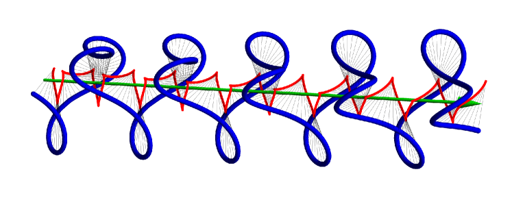
Figure 2: A bicycle geodesic in ${\mathbb{R}}^{3}.$ The front track is blue and the back track is red. The front track is also the trajectory of a Killing magnetic field, whose axis is marked in green.

Kirchhoff rods.

These are curves in ${\mathbb{R}}^{3}$ which are extrema of the total squared curvature (‘bending energy’) among curves with fixed end points, total torsion, and length. Accordingly, one defines the functional

$$\gamma\mapsto\int_{\gamma}\left(\kappa^{2}+\lambda_{1}\tau+\lambda_{2}\right)ds,$$

where $\lambda_{1},\lambda_{2}$ are Lagrange multipliers, and studies the associated variational equations. The result is a 4-parameter family of space curves (up to rigid motions), either straight lines or curves whose curvature $\kappa$ and torsion $\tau$, as functions of arc length, satisfy

$$\kappa^{\prime\prime}=\kappa\left[2a_{1}+\tau(\tau-a_{2})-\frac{\kappa^{2}}{2}\right],$$ (1)

$$\kappa^{2}(2\tau-a_{2})=a_{3},\$$ (2)

where $a_{1},a_{2},a_{3}\in{\mathbb{R}}$. The ODE (1) admits an ‘energy conservation law’,

$$(\kappa^{\prime})^{2}+\frac{1}{4}\left(\kappa^{2}-2a_{1}\right)^{2}+\kappa^{2}(\tau-a_{2})^{2}=(a_{4})^{2},$$ (3)

for some $a_{4}\in{\mathbb{R}}$. See for example [8, §4].

Remark 1.1.

Note that equation (1) cannot be replaced with (3), since there are solutions of (2)-(3) with constant $\kappa,\tau$ which are not solutions of (1)-(2); however, for solutions with non-vanishing $\kappa^{\prime}$, equations (1) and (3) are equivalent.

Among Kirchhoff rods, elastic curves are those with $a_{2}=0$. Planar Kirchhoff rods, i.e., those with $\tau=0$, are planar elastic curves, satisfying $a_{2}=a_{3}=0$. See Figure 3.

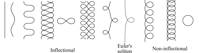
Figure 3: The family of planar elastic curves.

One can use equations (1)-(3) to write a single ODE for $u:=\kappa^{2}$ of the form $(u^{\prime})^{2}=P(u)$, where $P$ is a cubic polynomial. It follows that $u,$ and therefore $\kappa$ and $\tau$, are elliptic functions (doubly periodic in the complex domain) so that the curves themselves are quasi-periodic, i.e., ${\bf x}(t+T)=M({\bf x}(t)),$ for some $T>0$, $M\in\mathrm{Iso}({\mathbb{R}}^{3})$ and all $t$. The isometry $M$ is called the monodromy of the geodesic.

Another useful characterization of Kirchhoff rods is as the trajectories of a charged particle in a Killing magnetic field; that is, the solutions ${\bf x}(t)$ of

$${\bf x}^{\prime\prime}={\bf x}^{\prime}\times{\bf K},\ \mbox{where }{\bf K}=({\bf x}-{\bf x}_{1})\times{\bf p}+\delta{\bf p}$$ (4)

for some fixed ${\bf p},{\bf x}_{1}\in{\mathbb{R}}^{3}$, $\delta\in{\mathbb{R}}$. The vector field ${\bf K}$ is called ‘Killing’, or an ‘infinitesimal isometry’, since it generates screw-like rigid motions about a fixed line, the line passing through ${\bf x}_{1}$ in the direction of ${\bf p}$. Note that for $\delta=0$ and ${\bf x}^{\prime}(0)\|{\bf p}$ the trajectory is a planar elastica. See [3, 4].

The main result.

Theorem 1.

1. The front and back tracks of each bicycling geodesic in ${\mathbb{R}}^{n}$, $n\geq 3$, are contained in a 3-dimensional affine subspace.

2. Front tracks of bicycling geodesics in ${\mathbb{R}}^{3}$ are either straight lines or curves whose curvature and torsion functions satisfy

   $$\kappa^{\prime\prime}=\kappa\left[\tau(\tau-b)+\frac{1+a^{2}-\kappa^{2}}{2}\right],$$

   $$\kappa^{2}(2\tau-b)=b(a^{2}-1),$$

   and such that

   $$(\kappa^{\prime})^{2}+\frac{1}{4}\left(1+a^{2}-\kappa^{2}\right)^{2}+\kappa^{2}(\tau-b)^{2}=a^{2}+b^{2},$$

   where $a,b\in{\mathbb{R}}$. These curves comprise a 2-parameter subfamily of Kirchhoff rods, solutions to equations (1)-(3), with parameter values

   $$a_{1}={1+a^{2}\over 2},\ a_{2}=b,\ a_{3}=b(a^{2}-1),\ a_{4}=\sqrt{a^{2}+b^{2}}.$$ (5)

3. A unit speed bicycle path $({\bf x}(t),{\bf y}(t))$ in ${\mathbb{R}}^{3}$, that is,

   $$|{\bf x}^{\prime}(t)|=1,\ |{\bf x}(t)-{\bf y}(t)|=1,\ {\bf y}^{\prime}(t)\|({\bf x}(t)-{\bf y}(t))\mbox{ for all }t,$$

   with initial conditions ${\bf x}_{0},{\bf x}^{\prime}_{0},{\bf y}_{0}\in{\mathbb{R}}^{3}$, is a bicycling geodesic if and only if the front track ${\bf x}(t)$ is either a unit circle with ${\bf y}(t)$ fixed at its center, or a solution to equations (4) with

   $${\bf p}\neq 0,\ {\bf v}_{0}\cdot({\bf x}^{\prime}_{0}-{\bf p})=0,\ {\bf x}_{1}={\bf y}_{0}+{({\bf x}^{\prime}_{0}\times{\bf v}_{0})\times{\bf p}\over|{\bf p}|^{2}},\ \delta={({\bf x}^{\prime}_{0}\times{\bf v}_{0})\cdot{\bf p}\over|{\bf p}|^{2}}.$$

   The parameters $a,b$ of the previous item are given by

   $$a^{2}+b^{2}=|{\bf p}|^{2},\ b=-({\bf x}_{0}^{\prime}\times{\bf v}_{0})\cdot{\bf p}.$$

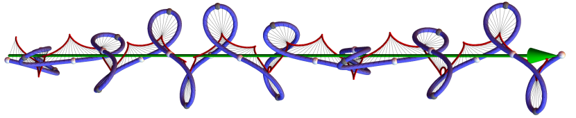
Figure 4: A bicycling geodesic with front track (blue) of constant torsion (the curvature function is that of a planar inflectional elastic curve). Points with vanishing $\kappa$ (inflection points) are marked with light marks, maxima and minima of $\kappa$ are marked with dark marks. The back track is red. The green axis is the symmetry axis of the associated monodromy and the magnetic field ${\bf K}$ of equation (4).

Additional results.

A detailed description of bicycling geodesic involves the following results proved in Section 3:

• Front tracks of planar geodesics are the solutions of Theorem 1(b) with $b=0$, or unit circles ($a=0$). As shown in [1], these front tracks are non-inflectional elasticae, see Proposition 3.5(a) and Figure 3.

• Solutions with $|a|=1$ correspond to front tracks with constant torsion $\tau=b/2,$ and whose curvature is that of planar inflectional elasticae. See Proposition 3.5(b) and Figure 4.

• Each non-planar geodesic front track comes in a ‘fixed size’. That is, no two such curves are related by a similarity transformation. This is unlike the planar case, where each front track, except circle, straight line and Euler soliton, come in two ‘sizes’, ‘wide’ and ‘narrow’, see [1, §4]. The closest thing to it, for non-planar geodesic front tracks, is a ‘torsion-shift-plus-rescaling’ transformation, see Proposition 3.10.

• The only globally minimizing bicycle geodesics are the planar minimizers, i.e., those geodesics whose front tracks are either a line or an Euler’s soliton. See Proposition 3.18.

• There are no closed bicycling geodesics except those with circular front tracks. See Proposition 3.6.

• Bicycle geodesics, like all Kirchhoff rods, can be expressed explicitly in terms of elliptic functions. See the Appendix.

• Back tracks of bicycling geodesic are determined by their front tracks. (Exception: linear front tracks.) See Proposition 3.7.

• Given a rear bicycle track, bicycle correspondence between front tracks is the result of reversing the direction of the bicycle frame, see [2]. Bicycle correspondence defines an isometric involution on the bicycle configuration space, acting on the front and back tracks of geodesics by an isometry whose second iteration is the monodromy of the tracks involved. See Proposition 3.14.

Acknowledgments.

We are grateful to David Singer for a suggestion that led to Proposition 3.10. The referee helped us realize that Section 2.3 was needed. In writing it, conversations with Richard Montgomery helped us understand the mysteries of abnormal geodesics in sub-Riemannian geometry and his wonderful book [10]. GB acknowledges support from CONACYT Grant A1-S-45886. ST was supported by NSF grant DMS-2005444.

2 Proof of Theorem 1

2.1 A sub-Riemannian  reformulation

We start by reformulating bicycle paths and geodesics in the language of sub-Riemannian geometry. Our main reference here is Chapter 5 of the book [10].

Denote by ${\bf v}:={\bf x}-{\bf y}\in S^{n-1}$ the frame direction and by

$$Q:=\{({\bf x},{\bf v})\,|\,|{\bf v}|=1\}={\mathbb{R}}^{n}\times S^{n-1}$$

the bicycling configuration space. The no-skid condition defines an $n$-distribution ${\mathscr{D}}$ on $Q,$ that is, a rank $n$ sub-bundle ${\mathscr{D}}\subset TQ$, so that bicycle paths are curves in $Q$ tangent everywhere to ${\mathscr{D}}$.

Lemma 2.1.

${\mathscr{D}}$ consists of vectors $({\bf x}^{\prime},{\bf v}^{\prime})\in T_{({\bf x},{\bf v})}Q$ satisfying

$${\bf v}^{\prime}={\bf x}^{\prime}-({\bf x}^{\prime}\cdot{\bf v}){\bf v}.$$ (6)

The proof appeared before, e.g., in Proposition 2.1 of [2], or Lemma 4.1 of [1]. Since the proof is quite short, and our notation here differs slightly from that of these references, we reproduce it here.

Proof.

Let $({\bf x}(t),{\bf v}(t))$ be a path in $Q$ and ${\bf x}^{\prime}_{\|}:=({\bf x}^{\prime}\cdot{\bf v}){\bf v}$ the orthogonal projection of the front track velocity on the frame direction. The no-skid condition is then ${\bf y}^{\prime}={\bf x}^{\prime}_{\|}.$ From ${\bf v}={\bf x}-{\bf y}$ it follows that ${\bf y}^{\prime}={\bf x}^{\prime}_{\|}$ is equivalent to ${\bf v}^{\prime}={\bf x}^{\prime}-{\bf x}^{\prime}_{\|},$ which is equation (6). ∎

The sub-Riemannian length of a vector $({\bf x}^{\prime},{\bf v}^{\prime})\in{\mathscr{D}}$ is, by definition, the length $|{\bf x}^{\prime}|$ of its projection to ${\mathbb{R}}^{n}$. This defines a sub-Riemannian  structure $(Q,{\mathscr{D}},g)$, where $g$ is a positive definite quadratic form on ${\mathscr{D}}$, the restriction to ${\mathscr{D}}$ of the pull-back to $Q$ of the standard riemannian metric on ${\mathbb{R}}^{n}$ under the ‘front wheel’ projection $Q\to{\mathbb{R}}^{n}$, $({\bf x},{\bf v})\mapsto{\bf x}.$ In this language, bicycle geodesics are the geodesics of $(Q,{\mathscr{D}},g)$, that is, curves in $Q$ tangent to ${\mathscr{D}}$ whose length between any two fixed points on them is critical among curves in $Q$ tangent to ${\mathscr{D}}$ whose end points are these fixed points. In fact, as in the Riemannian case, if the geodesic arc is sufficiently short then it is minimizing between its endpoints. See Theorem 1.14 on page 9 of [10].

Now in general, sub-Riemannian geodesics are either normal or abnormal. Normal geodesics always exist and are given by solutions of an analog of the usual geodesic equations in Riemannian geometry. We shall next derive these equations for bicycle geodesics in Lemma 2.4 below. Abnormal sub-Riemannian geodesics do not have a Riemannian analog and are harder to pin down. We shall later show, in section 2.3, that abnormal bicycle geodesics in fact do not exist, i.e., all bicycle geodesics satisfy the geodesic equations, see Corollary 2.20.

2.2 The bicycle geodesics equations

The (normal) geodesic equations on a sub-Riemannian  manifold $(Q,{\mathscr{D}},g)$ are derived via a Hamiltonian formalism, as follows.

One fixes an orthonormal frame $\xi_{i}$ for ${\mathscr{D}}$ and let $P_{i}:T^{*}Q\to{\mathbb{R}}$ be the associated fiber-wise linear momentum functions,

$$P_{i}(\alpha):=\alpha(\xi_{i}),\ \alpha\in T^{*}Q.$$

One forms the Hamiltonian $H:=(1/2)\sum_{i}(P_{i})^{2}$ on $T^{*}Q$ and the associated Hamiltonian vector field $X$ (with respect to the standard symplectic structure on $T^{*}Q$). The sub-Riemannian normal geodesics are then the projection to $Q$ of the integral curves of $X$. See Definition 1.13 on page 8 of [10]. We shall now follow this recipe in our case.

Let $\partial_{x_{i}}$ be the standard basis in ${\mathbb{R}}^{n}$ and ${\bf n}=\sum_{j=1}^{n}v_{j}\partial_{v_{j}}$ be the unit normal along $S^{n-1}\subset{\mathbb{R}}^{n}.$ Then, by Lemma 2.1, the vectors

$$\xi_{i}:=\partial_{x_{i}}+\partial_{v_{i}}-v_{i}{\bf n},\ i=1,\ldots,n,$$ (7)

form an orthonormal basis of ${\mathscr{D}}$.

Using the Euclidean structure on ${\mathbb{R}}^{n}$ we identify

$$T^{*}({\mathbb{R}}^{n}\times{\mathbb{R}}^{n})=T({\mathbb{R}}^{n}\times{\mathbb{R}}^{n}),\ T^{*}Q=TQ,$$

so that $T^{*}Q\subset T^{*}({\mathbb{R}}^{n}\times{\mathbb{R}}^{n})$ is a symplectic submanifold. Let $p_{i},r_{i}$ be the momenta coordinates on $T^{*}({\mathbb{R}}^{n}\times{\mathbb{R}}^{n})$ dual to $x_{i},v_{i}$; that is, if $\alpha\in T^{*}({\mathbb{R}}^{n}\times{\mathbb{R}}^{n})$ then $p_{i}(\alpha):=\alpha(\partial_{x_{i}}),\ r_{i}(\alpha):=\alpha(\partial_{v_{i}}).$ We shall use the same letters $x_{i},v_{i},p_{i},r_{i}$ to denote the restriction of these functions to $T^{*}Q$.

Notation. We shall use a vector notation throughout:

$$\begin{split}{\bf a}=(a_{1},\ldots,a_{n}),\ {\bf a}\cdot{\bf b}=\sum_{i=1}^{n}a_{i}b_{i},\ {\bf a}\,\partial_{\bf x}=\sum_{i=1}^{n}a_{i}\partial_{x_{i}},\\ \omega=d{\bf x}\wedge d{\bf p}+d{\bf v}\wedge d{\bf r}=\sum_{i=1}^{n}dx_{i}\wedge dp_{i}+dv_{i}\wedge dr_{i},\end{split}$$

etc.

Lemma 2.2.

$T^{*}Q\subset T^{*}({\mathbb{R}}^{n}\times{\mathbb{R}}^{n})$ is given, in the coordinates ${\bf x},{\bf v},{\bf p},{\bf r}$, by

$${\bf v}\cdot{\bf v}=1,\quad{\bf r}\cdot{\bf v}=0.$$

Proof.

Let $({\bf x},{\bf v})\in Q$, so that ${\bf v}\cdot{\bf v}=1$, and

$$\alpha={\bf p}d{\bf x}+{\bf r}d{\bf v}\in T^{*}_{({\bf x},{\bf v})}({\mathbb{R}}^{n}\times{\mathbb{R}}^{n}).$$

Then $\alpha\in T^{*}Q$ if and only if the corresponding vector,

$$X={\bf p}\partial_{\bf x}+{\bf r}\partial_{\bf v}\in T_{({\bf x},{\bf v})}({\mathbb{R}}^{n}\times{\mathbb{R}}^{n}),$$

satisfies $X({\bf v}\cdot{\bf v})=0$. That is, $0={\bf v}d{\bf v}(X)={\bf r}\cdot{\bf v}=0.$ ∎

Lemma 2.3.

$P_{i}=p_{i}+r_{i}$ on $T^{*}Q$. Thus

$$H={1\over 2}|{\bf p}+{\bf r}|^{2}={1\over 2}\sum_{i=1}^{n}(p_{i}+r_{i})^{2}.$$ (8)

Proof.

Let $\alpha={\bf p}d{\bf x}+{\bf r}d{\bf v}\in T^{*}Q$. By equation (7), $P_{i}(\alpha):=\alpha(\xi_{i})=p_{i}+r_{i}+v_{i}({\bf v}\cdot{\bf r}).$ By the previous lemma, the last term vanishes. ∎

Lemma 2.4.

The Hamiltonian equations on $T^{*}Q$, corresponding to the Hamiltonian (8), are

$${\bf x}^{\prime}={\bf p}+{\bf r},$$ (9)

$${\bf v}^{\prime}={\bf p}+{\bf r}-({\bf v}\cdot{\bf p}){\bf v},$$

$${\bf p}^{\prime}=0,$$

$${\bf r}^{\prime}=({\bf v}\cdot{\bf p}){\bf r}-[{\bf r}\cdot({\bf r}+{\bf p})]{\bf v},$$

with ${\bf v}\cdot{\bf v}=1,$ ${\bf r}\cdot{\bf v}=0$.

Proof.

Let $X$ be the Hamiltonian vector field on $T^{*}Q$,

$$X={\bf x}^{\prime}\partial_{\bf x}+{\bf v}^{\prime}\partial_{\bf v}+{\bf p}^{\prime}\partial_{\bf p}+{\bf r}^{\prime}\partial_{\bf r},$$

where ${\bf x}^{\prime},{\bf v}^{\prime},{\bf p}^{\prime},{\bf r}^{\prime}$ are unknown vectors. We have

$$dH=i_{X}\omega,$$ (10)

where $\omega=d{\bf x}\wedge d{\bf p}+d{\bf v}\wedge d{\bf r}$ is the symplectic form.

Now

$$i_{X}\omega={\bf x}^{\prime}d{\bf p}+{\bf v}^{\prime}d{\bf r}-{\bf p}^{\prime}d{\bf x}-{\bf r}^{\prime}d{\bf v}$$

and, by equation (8),

$$dH=({\bf p}+{\bf r})(d{\bf p}+d{\bf r}).$$

Note that equation (10) is an equality between 1-forms on $T^{*}Q$, the restrictions of both sides of (10) to $T^{*}Q$. By Lemma 2.2, the kernel of this restriction is spanned by ${\bf v}d{\bf v},{\bf r}d{\bf v}+{\bf v}d{\bf r}$. Thus, equation (10) amounts to the existence of functions $\lambda,\mu$ on $T^{*}Q$ such that

$$\begin{split}({\bf p}+{\bf r})(d{\bf p}+d{\bf r})=&\ {\bf x}^{\prime}d{\bf p}+{\bf v}^{\prime}d{\bf r}-{\bf p}^{\prime}d{\bf x}-{\bf r}^{\prime}d{\bf v}\\ &\qquad+\lambda{\bf v}d{\bf v}+\mu({\bf r}d{\bf v}+{\bf v}d{\bf r}).\end{split}$$

Equating coefficients, we obtain

$${\bf x}^{\prime}={\bf p}+{\bf r},\ {\bf v}^{\prime}={\bf p}+{\bf r}-\mu{\bf v},\ {\bf p}^{\prime}=0,\ {\bf r}^{\prime}=\lambda{\bf v}+\mu{\bf r}.$$ (11)

Furthermore, since $X$ is a vector field on $T^{*}Q$, ${\bf v}d{\bf v},{\bf r}d{\bf v}+{\bf v}d{\bf r}$ vanish on $X$, hence

$${\bf v}\cdot{\bf v}^{\prime}=0,\ {\bf v}^{\prime}\cdot{\bf r}+{\bf v}\cdot{\bf r}^{\prime}=0.$$

Dotting the second equation of (11) with ${\bf v}$, one obtains

$$0={\bf v}\cdot{\bf v}^{\prime}={\bf v}\cdot({\bf p}+{\bf r}-\mu{\bf v})={\bf v}\cdot{\bf p}-\mu,$$

hence $\mu={\bf v}\cdot{\bf p}.$ Dotting the 4th equation of (11) with ${\bf v}$ one obtains ${\bf v}\cdot{\bf r}^{\prime}={\bf v}\cdot(\lambda{\bf v}+\mu{\bf r})=\lambda,$ hence

$$\lambda=-{\bf v}^{\prime}\cdot{\bf r}=-({\bf p}+{\bf r}-\mu{\bf v})\cdot{\bf r}=-({\bf p}+{\bf r})\cdot{\bf r}.$$

Substituting these values of $\lambda,\mu$ in equations (11), we obtain equations (9). ∎

Lemma 2.5.

The tri-vector ${\bf p}\wedge{\bf v}\wedge{\bf x}^{\prime}$ is constant along solutions of equations (9).

Proof.

Using equations (9),

$$\begin{split}({\bf p}\wedge{\bf v}\wedge{\bf x}^{\prime})^{\prime}&=({\bf p}\wedge{\bf v}\wedge{\bf r})^{\prime}={\bf p}\wedge{\bf v}^{\prime}\wedge{\bf r}+{\bf p}\wedge{\bf v}\wedge{\bf r}^{\prime}\\ &=-({\bf v}\cdot{\bf p}){\bf p}\wedge{\bf v}\wedge{\bf r}+({\bf v}\cdot{\bf p}){\bf p}\wedge{\bf v}\wedge{\bf r}=0,\end{split}$$

as needed. ∎

Corollary 2.6 (Part (a) of Theorem 1).

For any normal bicycling geodesic (projection to $Q$ of a solution of equations (9)), the front and back tracks ${\bf x}(t),{\bf v}(t)$ are contained in the affine space passing through ${\bf x}_{0}$, parallel to the linear subspace spanned by ${\bf x}^{\prime}_{0},{\bf v}_{0},{\bf p}.$

Remark 2.7.

One can give also a geometric argument for Corollary 2.6. Let $({\bf x}(t),{\bf y}(t)),\ t\in[t_{0},t_{1}],$ be a unique minimizing geodesic (we assume that the interval $[t_{0},t_{1}]$ is small enough). Generically, the points ${\bf x}(t_{0}),{\bf y}(t_{0}),{\bf x}(t_{1}),{\bf y}(t_{1})$ span a 3-dimensional affine space, and the reflection in this subspace induces an isometry of the configuration space $Q$. If the geodesic is not contained in this 3-space, then its reflection is another minimizing geodesic, contradicting its uniqueness.

Another consequence of equations (9) is

Corollary 2.8.

1. ${\bf x}^{\prime}\cdot{\bf x}^{\prime}=2H$ is constant along solutions of equations (9).

2. If $({\bf x}(t),{\bf v}(t),{\bf p},{\bf r}(t))$ is a solution then so is $({\bf x}(\lambda t),{\bf v}(\lambda t),\lambda{\bf p},\lambda{\bf r}(\lambda t)$ for all $\lambda\neq 0.$

We now proceed to proving parts (b), (c) of Theorem 1. By the last corollaries, we shall assume henceforth that $n=3$ and $|{\bf x}^{\prime}(t)|=1$ (arc length parametrization of the front track).

Lemma 2.9.

For any solution of equations (9):

1. $b:={\bf p}\cdot({\bf v}\times{\bf x}^{\prime})$ is constant.

2. $|b|\leq|{\bf p}|,$ with equality if and only if the front track is a unit circle, with the back wheel staying fixed at the center of the circle.

3. If a geodesic has a front track which is a straight line, ${\bf x}^{\prime\prime}=0$, then $b=0$, $|{\bf p}|=1$. (The converse is not true, because the Euler soliton as the front track also corresponds to these values, see Proposition 3.5 below).

4. Equations (9) are equivalent to

   $${\mathbf{T}}^{\prime}={\mathbf{T}}\times{\bf K},\ {\bf v}^{\prime}={\mathbf{T}}-({\bf v}\cdot{\bf p}){\bf v},\quad$$ (12)

   where

   $${\mathbf{T}}={\bf x}^{\prime},\ {\bf K}={\bf r}\times{\bf v}=({\mathbf{T}}-{\bf p})\times{\bf v},\ {\bf p}=const,|{\mathbf{T}}|=|{\bf v}|=1,\ {\bf r}\cdot{\bf v}=0.$$

Proof.

(i) follows from Lemma 2.5.

(ii) By the Cauchy-Schwartz inequality, $|b|=|{\bf p}\cdot({\bf v}\times{\bf x}^{\prime})|\leq|{\bf p}||{\bf v}||{\bf x}^{\prime}|=|{\bf p}|,$ with equality if either ${\bf p}=0$ or ${\bf p}\neq 0$ and ${\bf x}^{\prime},{\bf v},{\bf p}$ are pairwise orthogonal. In the first case ${\bf x}^{\prime}={\bf r}$, hence is perpendicular to ${\bf v}$, and in both cases, setting ${\mathbf{T}}={\bf x}^{\prime}$, equations (9) give ${\mathbf{T}}^{\prime\prime}=-{\mathbf{T}},\ {\bf v}=-{\mathbf{T}}^{\prime},$ and claim (ii) follows.

(iii) The first equation of (9) implies that ${\bf r}={\bf x}^{\prime}-{\bf p}=const,$ thus, by the 4th equation, $({\bf v}\cdot{\bf p}){\bf r}=({\bf r}\cdot{\bf x}^{\prime}){\bf v}.$ Dotting with ${\bf r}$, we get $({\bf v}\cdot{\bf p})|{\bf r}|^{2}=0,$ so either ${\bf v}\cdot{\bf p}=0$ or ${\bf r}=0$. If ${\bf v}\cdot{\bf p}=0$ then by the 3rd equation, ${\bf v}^{\prime}={\bf x}^{\prime},$ so ${\bf v}={\bf v}_{0}+t{\bf x}^{\prime}$, which is impossible since $|{\bf v}|=|{\bf x}^{\prime}|=1$. Hence ${\bf r}=0$, so ${\bf p}={\bf x}^{\prime}$, which implies that $b={\bf p}\cdot({\bf v}\times{\bf x}^{\prime})={\bf x}^{\prime}\cdot({\bf v}\times{\bf x}^{\prime})=0$ and $|{\bf p}|=|{\bf x}^{\prime}|=1$, as needed.

(iv) The 3rd equation of (9) gives ${\mathbf{T}}^{\prime}=({\bf v}\cdot{\bf p}){\bf r}-({\bf r}\cdot{\mathbf{T}}){\bf v}.$ By the vector identity

$${\bf a}\times({\bf b}\times{\bf c})=({\bf a}\cdot{\bf c}){\bf b}-({\bf a}\cdot{\bf b}){\bf c},$$ (13)

this is equivalent to ${\mathbf{T}}^{\prime}={\mathbf{T}}\times({\bf r}\times{\bf v}).$ The second equation of (12) is immediate from the first and second equations of (9). ∎

Remark 2.10.

The front track of a bicycling geodesic with ${\bf p}=0$ is thus a unit circle with the back track fixed at its center. From here on, unless otherwise mentioned, we will only consider bicycling geodesics with ${\bf p}\neq 0$.

Proposition 2.11 (Part c of Theorem 1).

A unit speed bicycle path $({\bf x}(t),{\bf v}(t))$ in ${\mathbb{R}}^{3}$ with initial conditions ${\bf x}_{0},{\bf x}^{\prime}_{0},{\bf v}_{0}$ is a bicycling geodesic (a solution to equations (12)) with ${\bf p}\neq 0$ if and only if ${\bf x}(t)$ is a solution to

$${\bf x}^{\prime\prime}={\bf x}^{\prime}\times{\bf K},\ \mbox{ where }{\bf K}=({\bf x}-{\bf x}_{1})\times{\bf p}+\delta{\bf p},$$ (14)

and

$${\bf v}_{0}\cdot({\bf x}^{\prime}_{0}-{\bf p})=0,\ {\bf x}_{1}={\bf y}_{0}+{({\bf x}^{\prime}_{0}\times{\bf v}_{0})\times{\bf p}\over|{\bf p}|^{2}},\ \delta={({\bf x}^{\prime}_{0}\times{\bf v}_{0})\cdot{\bf p}\over|{\bf p}|^{2}}=-{b\over|{\bf p}|^{2}},$$

where ${\bf y}_{0}={\bf x}_{0}-{\bf v}_{0}$ is the initial back track position. See Figure 5.

Figure 5:

Proof.

From equations (12),

$${\bf x}^{\prime\prime}={\bf x}^{\prime}\times{\bf K},$$ (15)

where ${\bf K}:={\bf r}\times{\bf v}$ and ${\bf r}={\bf x}^{\prime}-{\bf p}.$ By equations (9),

$$\begin{split}{\bf K}^{\prime}&={\bf r}^{\prime}\times{\bf v}+{\bf r}\times{\bf v}^{\prime}=({\bf v}\cdot{\bf p}){\bf r}\times{\bf v}+{\bf r}\times[{\bf p}-({\bf v}\cdot{\bf p}){\bf v}]={\bf r}\times{\bf p}\\ &=({\bf x}\times{\bf p})^{\prime}.\end{split}$$ (16)

Consequently,

$${\bf K}-{\bf x}\times{\bf p}={\bf r}_{0}\times{\bf v}_{0}-{\bf x}_{0}\times{\bf p},$$

or

$${\bf K}=({\bf x}-{\bf y}_{0})\times{\bf p}+{\bf x}_{0}^{\prime}\times{\bf v}_{0}.$$ (17)

Since ${\bf p}\neq 0$, we may decompose orthogonally

$${\bf x}_{0}^{\prime}\times{\bf v}_{0}={\bf p}\times{\bf a}+\delta{\bf p},$$ (18)

for some ${\bf a}\perp{\bf p}$ and $\delta\in{\mathbb{R}}$. Then

$$({\bf x}_{0}^{\prime}\times{\bf v}_{0})\times{\bf p}=|{\bf p}|^{2}{\bf a},\ ({\bf x}_{0}^{\prime}\times{\bf v}_{0})\cdot{\bf p}=|{\bf p}|^{2}\delta,$$

hence

$${\bf a}={({\bf x}_{0}^{\prime}\times{\bf v}_{0})\times{\bf p}\over|{\bf p}|^{2}},\ \delta={({\bf x}_{0}^{\prime}\times{\bf v}_{0})\cdot{\bf p}\over|{\bf p}|^{2}}=-{b\over|{\bf p}|^{2}}.$$ (19)

Equations (14) now follow from (15)-(19) by taking ${\bf x}_{1}:={\bf y}_{0}+{\bf a}$.

Conversely, the magnetic field ${\bf K}$ and initial conditions for its trajectory are defined using only the initial conditions for the bicycling geodesic’s front track. Since they satisfy the same equations of motion (equation (12)), such magnetic field trajectories coincide with the bicycling geodesics.∎

Let ${\mathbf{T}},{\mathbf{N}},{\mathbf{B}}$ be the Frenet-Serret frame along a non-linear front track ${\bf x}(t)$, and $\kappa,\tau$ the curvature and torsion functions, respectively. That is,

$${\bf x}^{\prime}={\mathbf{T}},\ {\mathbf{T}}^{\prime}=\kappa{\mathbf{N}},\ {\mathbf{N}}^{\prime}=-\kappa{\mathbf{T}}+\tau{\mathbf{B}},\ {\mathbf{B}}^{\prime}=-\tau{\mathbf{N}},$$ (20)

where ${\mathbf{B}}={\mathbf{T}}\times{\mathbf{N}}$ (the Frenet-Serret equations).

Remark 2.12.

The Frenet-Serret frame is usually defined via formulas (20) along a regular curve ${\bf x}(t)$ in ${\mathbb{R}}^{3}$, parametrized by arc length, with non-vanishing acceleration ${\bf x}^{\prime\prime}$, by adding the condition $\kappa>0$. If one does not add the last condition, then the frame is well defined only up to the involution

$$({\mathbf{T}},{\mathbf{N}},{\mathbf{B}},\kappa,\tau)\mapsto({\mathbf{T}},-{\mathbf{N}},-{\mathbf{B}},-\kappa,\tau).$$

For analytic curves, as is our case (the right hand side of equations (9) are quadratic polynomials), ${\bf x}^{\prime\prime}$ either vanishes identically, in which case it is a line, or vanishes at isolated points, the inflection points of the curve.

In the latter case, by looking at the Taylor series of ${\bf x}(t)$ around an inflection point, say ${\bf x}(0)$, one sees that that the Frenet-Serret frame extends analytically to these points, so equations (20) still hold, but $\kappa$ may change sign at the inflection point. For example, if ${\bf x}^{\prime\prime\prime}(0)\neq 0$, then $\kappa^{\prime}(0)\neq 0$.

That is, any analytic non-linear regular curve ${\bf x}(t)$ admits exactly two Frenet-Serret frames, $({\mathbf{T}},{\mathbf{N}},{\mathbf{B}},\kappa,\tau)$ and $({\mathbf{T}},-{\mathbf{N}},-{\mathbf{B}},-\kappa,\tau)$, both satisfying the Frenet-Serret equations (20), but if the $\kappa$ has variable sign there is no natural way to choose one of the frames. This situation actually occurs for some of the solutions of equations (9), as we shall see later (the constant torsion solutions, see Proposition 3.5 below).

In summary, in what follows, whenever we mention “the Frenet-Serret frame”, we implicitly refer to either choice of these frames in case $\kappa$ has a variable sign. One can check that all equations involving the frame are invariant under the involution $({\mathbf{T}},{\mathbf{N}},{\mathbf{B}},\kappa,\tau)\mapsto({\mathbf{T}},-{\mathbf{N}},-{\mathbf{B}},-\kappa,\tau)$. For more details on inflection points of analytic space curves see [12], or pages 41-43 of [6].

Lemma 2.13.

For any non-linear geodesic front track,

$${\bf p}={1+a^{2}-\kappa^{2}\over 2}{\mathbf{T}}-\kappa^{\prime}{\mathbf{N}}-\kappa(\tau-b){\mathbf{B}}=const.,$$ (21)

where $a^{2}:=|{\bf p}|^{2}-b^{2}$ (see Lemma 2.9).

Proof.

We compute each of the coefficients ${\bf p}\cdot{\mathbf{T}},{\bf p}\cdot{\mathbf{N}},{\bf p}\cdot{\mathbf{B}}$. Recall from (12) and (16) that for ${\bf K}:={\bf r}\times{\bf v}$ we have

$${\mathbf{T}}^{\prime}={\mathbf{T}}\times{\bf K},\quad{\bf K}^{\prime}={\mathbf{T}}\times{\bf p}.$$ (22)

Now, since ${\bf r}={\mathbf{T}}-{\bf p}$ and $b={\bf p}\cdot({\bf v}\times{\mathbf{T}})$, we have ${\mathbf{T}}\cdot{\bf K}={\mathbf{T}}\cdot({\bf r}\times{\bf v})=-b$. Using again the vector identity (13),

$$\kappa{\mathbf{B}}={\mathbf{T}}\times{\mathbf{T}}^{\prime}={\mathbf{T}}\times({\mathbf{T}}\times{\bf K})=-b{\mathbf{T}}-{\bf K}.$$ (23)

It follows that $|{\bf K}|^{2}=b^{2}+\kappa^{2}$, and since ${\bf r}\cdot{\bf v}=0$, $|{\bf v}|=1$, we have:

$$b^{2}+\kappa^{2}=|{\bf K}|^{2}=|{\bf r}|^{2}=|{\mathbf{T}}-{\bf p}|^{2}=1-2{\mathbf{T}}\cdot{\bf p}+|{\bf p}|^{2},$$

yielding the expression for the first component, ${\mathbf{T}}\cdot{\bf p}$.

For the remaining components, using equations (22) and (13), one has

$${\mathbf{T}}^{\prime\prime} =({\mathbf{T}}\times{\bf K})^{\prime}=({\mathbf{T}}\times{\bf K})\times{\bf K}+{\mathbf{T}}\times({\mathbf{T}}\times{\bf p})$$

$$=\left({\mathbf{T}}\cdot{\bf p}-|{\bf K}|^{2}\right){\mathbf{T}}-b{\bf K}-{\bf p}.$$

On the other hand, by the Frenet-Serret equations,

$${\mathbf{T}}^{\prime\prime}=-\kappa^{2}{\mathbf{T}}+\kappa^{\prime}{\mathbf{N}}+\kappa\tau{\mathbf{B}}.$$

Dotting these two expressions for ${\mathbf{T}}^{\prime\prime}$ with ${\mathbf{N}}$, we obtain $\kappa^{\prime}=-b{\bf K}\cdot{\mathbf{N}}-{\bf p}\cdot{\mathbf{N}}$, while from (23) we have ${\bf K}\cdot{\mathbf{N}}=0$, so that ${\bf p}\cdot{\mathbf{N}}=-\kappa^{\prime}$, as needed.

Dotting the two expressions for ${\mathbf{T}}^{\prime\prime}$ with ${\mathbf{B}}$ we obtain $\kappa\tau=-b{\bf K}\cdot{\mathbf{B}}-{\bf p}\cdot{\mathbf{B}}$, while from (23) we have ${\bf K}\cdot{\mathbf{B}}=-\kappa$, so that ${\bf p}\cdot{\mathbf{B}}=-\kappa(\tau-b)$. ∎

Now we prove the second statement of Theorem 1.

Proposition 2.14.

Non-linear geodesic front tracks in ${\mathbb{R}}^{3}$ (solutions to equations (9)) are curves whose curvature and torsion functions satisfy

$$\kappa^{\prime\prime}=\kappa\left(\tau(\tau-b)+\frac{1+a^{2}-\kappa^{2}}{2}\right),$$ (24)

$$\kappa^{2}(2\tau-b)=b(a^{2}-1),$$ (25)

such that

$$(\kappa^{\prime})^{2}+\frac{1}{4}\left(1+a^{2}-\kappa^{2}\right)^{2}+\kappa^{2}(\tau-b)^{2}=a^{2}+b^{2},$$ (26)

where $a,b\in{\mathbb{R}}$.

Proof.

Equation (26) is obtained by taking the norm square of both sides of (21). Equation (25) is obtained by dotting (23) with ${\bf p}$,

$$b=-{\bf K}\cdot{\bf p}=b{\mathbf{T}}\cdot{\bf p}+\kappa{\mathbf{B}}\cdot{\bf p},$$

then substituting the values of ${\mathbf{T}}\cdot{\bf p},\ {\mathbf{B}}\cdot{\bf p}$ from equation (21). Equation (24) follows by differentiating (21):

$$0=\left(-\kappa^{\prime\prime}+\kappa\left[\tau(\tau-b)+\frac{1+a^{2}-\kappa^{2}}{2}\right]\right){\mathbf{N}}-\left(\kappa^{\prime}\tau+\left[\kappa(\tau-b)\right]^{\prime}\right){\mathbf{B}}.$$

The vanishing of the ${\mathbf{N}}$ component gives equation (24).

Note that the vanishing of the ${\mathbf{B}}$ component in the last equation does not give new information: multiplying the ${\mathbf{B}}$ component by $-2\kappa$, one obtains the derivative of $\kappa^{2}(2\tau-b)$, which vanishes by equation (25). ∎

2.3 Bicycle geodesics are normal

Here we show that all bicycle geodesics in $Q={\mathbb{R}}^{n}\times S^{n-1}$ are normal, that is, the projections to $Q$ of solutions to equations (9). Our main reference here is section 5.3 of [10].

For a general sub-Riemannian  structure $(Q,{\mathscr{D}},g)$, abnormal geodesics are singular curves of $(Q,{\mathscr{D}})$ (the definition of singular curves does not involve the sub-Riemannian metric $g$, see below). The converse is not true: a singular geodesic may happen to be normal [10, §5.3.3]. Thus, in order to show that all bicycle geodesics are normal, we will first find the singular curves of $(Q,{\mathscr{D}})$, then show that all geodesics among them are normal, i.e., can be lifted to parametrized curves in $T^{*}Q$ satisfying equations (9).

Singular curves of $(Q,{\mathscr{D}})$ are defined by considering first the annihilator ${\mathscr{D}}^{0}\subset T^{*}Q$, that is, the set of covectors vanishing on ${\mathscr{D}}$. A characteristic curve of ${\mathscr{D}}^{0}$ is a curve in ${\mathscr{D}}^{0}$ which does not intersect the zero section of ${\mathscr{D}}^{0}\to Q$ and whose tangent is in the kernel of the restriction of the canonical symplectic form of $T^{*}Q$ to ${\mathscr{D}}^{0}$. A singular curve of $(Q,{\mathscr{D}})$ is the projection to $Q$ of a characteristic curve of ${\mathscr{D}}^{0}$.

The case $n=2$ is special, since in this case ${\mathscr{D}}$, defined by the non-skid condition (6), is contact, which implies that ${\mathscr{D}}^{0}\subset T^{*}Q$ is symplectic (see [1, §4.1] and the example at the top of page 59 of [10]). Hence there are no characteristics and singular curves for $n=2$ so all geodesics are automatically normal. We thus assume henceforth that $n>2$.

Proposition 2.15.

Singular bicycle paths consist of curves $({\bf x}(t),{\bf v}(t))$ in $Q$ in which the back wheel ${\bf x}(t)-{\bf v}(t)\in{\mathbb{R}}^{n}$ is fixed and ${\bf v}(t)$ moves in $S^{n-1}$ perpendicular to some fixed ${\bf p}\neq 0$, ${\bf p}\cdot{\bf v}(t)=0.$

Proof.

We first determine ${\mathscr{D}}^{0}\subset T^{*}Q$. Recall from Lemma 2.2 that $T^{*}Q$ is given in the canonical coordinates ${\bf x},{\bf v},{\bf p},{\bf r}$ on $T^{*}({\mathbb{R}}^{n}\times{\mathbb{R}}^{n})$ by ${\bf v}\cdot{\bf v}=1,\ {\bf r}\cdot{\bf v}=0$.

Lemma 2.16.

${\mathscr{D}}^{0}$ is a $(3n-2)$-dimensional submanifold of $T^{*}Q$, given by ${\bf v}\cdot{\bf v}=1,\ {\bf r}\cdot{\bf v}=0,\ {\bf r}+{\bf p}=0$.

Proof.

Let

$$\alpha={\bf p}d{\bf x}+{\bf r}d{\bf v}\in T^{*}Q,\ X={\bf x}^{\prime}\partial_{\bf x}+{\bf v}^{\prime}\partial_{\bf v}\in{\mathscr{D}}.$$

By Lemma 2.1, ${\bf v}^{\prime}={\bf x}^{\prime}-({\bf x}^{\prime}\cdot{\bf v}){\bf v}$. Thus, using that ${\bf r}\cdot{\bf v}=0$ on $T^{*}Q$, $\alpha\in{\mathscr{D}}^{0}$ if and only if

$$0=\alpha(X)={\bf p}\cdot{\bf x}^{\prime}+{\bf r}\cdot\left[{\bf x}^{\prime}-({\bf x}^{\prime}\cdot{\bf v}){\bf v})\right]=({\bf p}+{\bf r})\cdot{\bf x}^{\prime}$$

for all ${\bf x}^{\prime}\in{\mathbb{R}}^{n}$. That is, ${\bf p}+{\bf r}=0$, as claimed.

To prove that $\dim({\mathscr{D}}^{0})=3n-2$, using the implicit function theorem, we show that $(1,0,{\bf 0})\in{\mathbb{R}}\times{\mathbb{R}}\times{\mathbb{R}}^{n}$ is a regular value of

$$({\bf x},{\bf v},{\bf p},{\bf r})\mapsto(|{\bf v}|^{2},{\bf r}\cdot{\bf v},{\bf r}+{\bf p}).$$

That is, for a fixed $({\bf x},{\bf v},{\bf p},{\bf r})\in{\mathscr{D}}^{0}$, $a,b\in{\mathbb{R}}$, ${\bf c}\in{\mathbb{R}}^{n},$ one needs to solve

$${\bf v}\cdot{\bf v}^{\prime}=a,\ {\bf r}\cdot{\bf v}^{\prime}+{\bf r}^{\prime}\cdot{\bf v}=b,\ {\bf r}^{\prime}+{\bf p}^{\prime}={\bf c}$$

for ${\bf v}^{\prime},{\bf p}^{\prime},{\bf r}^{\prime}\in{\mathbb{R}}^{n}.$ These equations are solved by ${\bf v}^{\prime}=a{\bf v},{\bf r}^{\prime}=b{\bf v},{\bf p}^{\prime}={\bf c}-b{\bf v}.$ ∎

Lemma 2.17.

$$\omega:=d{\bf x}\wedge d{\bf p}+d{\bf v}\wedge d{\bf r}\equiv(d{\bf x}-d{\bf v})\wedge d{\bf p}\not\equiv 0\mod{\mathscr{D}}^{0},$$

where equivalence of forms mod ${\mathscr{D}}^{0}$ means the equality of their restriction to ${\mathscr{D}}^{0}$.

Proof.

The first congruence follows from the equality ${\bf r}+{\bf p}=0$ on ${\mathscr{D}}^{0}$, proved in the last lemma. For $n>2$ we have, by the same lemma,

$$\dim({\mathscr{D}}^{0})=3n-2>2n={1\over 2}\dim\left[T^{*}({\mathbb{R}}^{n}\times{\mathbb{R}}^{n})\right],$$

so the restriction to ${\mathscr{D}}^{0}$ of $\omega$ (the canonical symplectic form of $T^{*}({\mathbb{R}}^{n}\times{\mathbb{R}}^{n})$) is non-vanishing. ∎

Next let

$$Y={\bf x}^{\prime}\partial_{\bf x}+{\bf v}^{\prime}\partial_{\bf v}+{\bf p}^{\prime}\partial_{\bf p}+{\bf r}^{\prime}\partial_{\bf r}$$

be a vector tangent to ${\mathscr{D}}^{0}$.

Lemma 2.18.

$Y$ is in the kernel of the restriction of $\omega$ to ${\mathscr{D}}^{0}$, $i_{Y}\omega\equiv 0\mod{\mathscr{D}}^{0}$, if and only if ${\bf p}^{\prime}={\bf r}^{\prime}={\bf x}^{\prime}-{\bf v}^{\prime}=0.$

Proof.

By Lemma 2.16,

$${\mathscr{D}}^{0}=\{{\bf v}\cdot{\bf v}=1,{\bf r}\cdot{\bf v}=0,{\bf p}+{\bf r}=0\},$$

hence tangency of $Y$ to ${\mathscr{D}}^{0}$ amounts to

$${\bf v}\cdot{\bf v}^{\prime}={\bf r}\cdot{\bf v}^{\prime}+{\bf v}\cdot{\bf r}^{\prime}=0,\ {\bf p}^{\prime}+{\bf r}^{\prime}=0,$$

thus

$$Y={\bf x}^{\prime}\partial_{\bf x}+{\bf v}^{\prime}\partial_{\bf v}+{\bf p}^{\prime}(\partial_{\bf p}-\partial_{\bf r}).$$

It follows that

$$i_{Y}\omega \equiv i_{Y}\left[(d{\bf x}-d{\bf v})\wedge d{\bf p}\right]=({\bf x}^{\prime}-{\bf v}^{\prime})d{\bf p}-{\bf p}^{\prime}(d{\bf x}-d{\bf v})\mod{\mathscr{D}}^{0}.$$

By Lemma 2.17, $d{\bf p}\wedge(d{\bf x}-d{\bf v})\not\equiv 0\mod{\mathscr{D}}^{0}.$ It follows that the restrictions of $d{\bf p},d{\bf x}-d{\bf v}$ to ${\mathscr{D}}^{0}$ are linearly independent, hence the vanishing of $i_{Y}\omega\mod{\mathscr{D}}^{0}$ is equivalent to the vanishing of ${\bf x}^{\prime}-{\bf v}^{\prime},{\bf p}^{\prime}.$ Since ${\bf r}^{\prime}=-{\bf p}^{\prime}$ for vectors tangent to ${\mathscr{D}}^{0}$, ${\bf r}^{\prime}$ vanishes as well. ∎

We can now complete the proof of Proposition 2.15. From the last lemma follows that characteristics of ${\mathscr{D}}^{0}$ are curves $({\bf x}(t),{\bf v}(t),{\bf p}(t),{\bf r}(t))$ where the back track ${\bf x}(t)-{\bf v}(t)$ is fixed, $|{\bf v}(t)|=1$, ${\bf r}(t)\cdot{\bf v}(t)=0$ and ${\bf p}(t)=-{\bf r}(t)$ is a non-zero constant vector. This projects to the stated curve in $Q$. ∎

Remark 2.19.

Proposition 2.15 is a special case of the following. Let $M$ be an $n$-dimensional manifold and $Q=S(TM)$ the spherized tangent bundle, consisting of pairs $(y,\ell)$, where $y\in M$ and $\ell$ is an oriented 1-dimensional subspace of $T_{y}M$. Define a rank $n$ distribution ${\mathscr{D}}\subset TQ$ whose integral curves are given by trajectories $(y(t),\ell(t))$ such that $\dot{y}(t)\in\ell(t)$ for all $t$. (One can think of $Q$ as the configuration space for bicycling on $M$, where $y$ is the back wheel placement, $\ell$ is the frame direction and ${\mathscr{D}}$ is the no-skid condition.) Note that the trajectories for which the back wheel is fixed, $y(t)=const.$, satisfy this condition trivially. Singular curves of $(Q,{\mathscr{D}})$ are then given by trajectories $(y(t),\ell(t))$ such that $y(t)=y$ is fixed and $\ell(t)$ varies in some fixed codimension 1 subspace of $T_{y}M$. Proposition 2.15 is the case of $M={\mathbb{R}}^{n}$ and actually implies the more general case since it is a local statement.

Corollary 2.20.

All bicycle geodesics are normal.

Proof.

By Proposition 2.15, the length of a singular bicycle path $({\bf x}(t),{\bf v}(t))$ is given by the length of the curve traced by ${\bf v}(t)$ on $S^{n-1}$. This length is critical when ${\bf v}(t)$ traces a spherical geodesic, i.e., an arc of a great circle on $S^{n-1}$ (the intersection of a 2-dimensional subspace of ${\mathbb{R}}^{n}$ with $S^{n-1}$). To show that this singular bicycle geodesic is normal we first reparametrize it by arc length, $|{\bf v}^{\prime}(t)|=1,$ then lift it to a solution of equations (9). Let ${\bf p}\neq 0$ be a vector perpendicular to the 2-plane spanned by ${\bf v}(t)$ and ${\bf r}(t):={\bf v}^{\prime}(t)-{\bf p}$. Then one can easily check that this defines a solution to equations (9). (Note that this lift is not a characteristic of ${\mathscr{D}}^{0}$, since for a characteristic ${\bf r}=-{\bf p}$ is constant.) ∎

3 Additional results

3.1 More about geodesic front tracks

In Theorem 1 we described front tracks of bicycling geodesics as a subfamily of Kirchhoff rods, parametrized by the two parameters $a,b$ in equations (24)-(26). Here we give more information on these curves.

Clearly, since $a$ appears in equations (24)-(26) only through $a^{2}$, it is enough to restrict to $a\geq 0$. Regarding $b$, we observe the following.

Lemma 3.1.

Reflection with respect to a plane or a point in ${\mathbb{R}}^{3}$ transforms a bicycling geodesic to another bicycling geodesic, with $(\kappa,\tau)\mapsto(\kappa,-\tau)$ and $(a,b)\mapsto(a,-b)$ in equations (24)-(26).

Proof.

The transformation of $\kappa,\tau$ follows from the Frenet-Serret equations (20). The transformation of $(a,b)$ then follows from equations (24)-(26). ∎

Therefore in what follows we will consider only the parameter values $a,b\geq 0$. See Figure 6.

Figure 6: The parameter space of bicycle geodesics.

Lemma 3.2.

All values of the parameters $a,b\geq 0$ in equations (24)-(26) occur among non-linear front tracks of bicycling geodesics.

Proof.

Let ${\bf v}_{0}:=(1,0,0)$, ${\bf x}^{\prime}_{0}:=(0,1,0)$, ${\bf p}:=(0,a,b)$. Then ${\bf v}_{0}\cdot({\bf x}_{0}^{\prime}-{\bf p})=0$, so these are admissible initial conditions for equations (14). The solution is a bicycling geodesic with ${\bf p}\cdot({\bf v}_{0}\times{\bf x}_{0}^{\prime})=b,$ $|{\bf p}|^{2}=a^{2}+b^{2},$ as needed. ∎

Proposition 3.3.

The curvature and torsion of non-linear geodesic front tracks, except for the Euler soliton ($a=1,b=0$), are periodic elliptic functions, varying in the following ranges (note the ‘doubling discontinuity’ of the range of $\kappa$ at $a=1$):

$$\begin{array}[]{ r ll l}{\rm(i)}&\mbox{For }0\leq a<1:&\quad-\frac{ab}{1+a}\ \leq\ \tau\ \leq\ \frac{ab}{1-a},&\qquad 1-a\leq\kappa\leq 1+a.\\ {\rm(ii)}&\mbox{For }a>1:&\quad\frac{ab}{1-a}\ \leq\ \tau\ \leq\ -\frac{ab}{1+a},&\qquad a-1\leq\kappa\leq a+1.\\ {\rm(iii)}&\mbox{For }a=1:&\quad\tau=b/2,&\qquad-2\leq\kappa\leq 2.\end{array}$$

Proof.

We use equation (25) to eliminate $\tau$ from equation (26). Then, setting $u:=\kappa^{2}$, we get

$$(u^{\prime})^{2}=P(u),$$ (27)

where

$$P(u)=(u+b^{2})\left[(1+a)^{2}-u\right]\left[u-(1-a)^{2}\right].$$

Equation (27) defines an oval in the $(u,u^{\prime})$ right half plane $u\geq 0$, an integral curve of the vector field $u^{\prime}\partial_{u}+{1\over 2}{dP\over du}\partial_{u^{\prime}}$. This vector filed does not vanish along the oval, since $P$ has no multiple roots for $a,b>0$ (except for $a=1,b=0$, the Euler soliton, see below). See Figure 7.

Figure 7: Phase portrait of equation (27), for $a=.5,b=1$ (inner oval), $a=1,b=1$ (outer oval).

Consequently, the phase point of equation (27) moves clockwise along this closed oval, so that $u$ oscillates periodically between the two non-negative roots $(1\pm a)^{2}$ of $P(u)$. For $a\neq 1$, since $u=\kappa^{2}\geq(1-a)^{2}>0$, this gives the claimed range of $\kappa$.

For $a=1$ one needs to be more careful. See the outer oval of Figure 7. The range of $u=\kappa^{2}$ is $[0,4]$, so $\kappa$ traverses the range $[0,2]$ as the phase point $(u,u^{\prime})$ goes once around the oval, starting and ending at $u=u^{\prime}=0$. Now $u=0$ implies $\kappa=0$, an inflection point of the front track, see Remark 2.12. By equation (26), at this point $(\kappa^{\prime})^{2}=b^{2}>0$, so $\kappa$ changes sign. Going once more around the oval, $\kappa$ now traverses the range $[-2,0]$.

The range of $\tau$ is obtained from that of $\kappa$ via equation (25). For example, when $a<1$, we have $\kappa^{2}(2\tau-b)=b(a^{2}-1)<0$, so that $2\tau-b<0$ and

$$(1+a)^{2}(2\tau+b)\leq b(1-a^{2})\leq(1-a)^{2}(2\tau+b)$$

since $(1-a)^{2}\leq\kappa^{2}\leq(1+a)^{2}$. Rearranging, we find $\frac{ab}{1-a}\leq\tau\leq-\frac{ab}{1+a}.$ The cases $a>1$ or $a=1$ are similar.

Since $P(u)$ is cubic in $u$, the solutions of (27) are elliptic functions (doubly periodic in the complex domain) and so are $\kappa(t)$ and $\tau(t)$. See the Appendix for explicit formulas. ∎

Corollary 3.4.

1. Non-linear front tracks with constant curvature are unit circles ($\kappa=1$, $a=0$).

2. Non-linear front tracks with constant torsion $\tau\neq 0$ correspond to $a=1$, $b=2\tau$.

3. Front tracks with $a>1$ have nowhere vanishing torsion, while those with $0<a<1$ have torsion of mixed signs. In both cases the curvature is non-vanishing (positive).

4. Front tracks with $a=1,b>0$ (constant non-vanishing torsion) have curvature of mixed sign.

5. Geodesic front tracks which are elastic curves ($a_{2}=0$ in equations (1)-(2)) are planar non-inflectional elasticae ($b=0$), as in Proposition 3.5(a) below. See Figure 3.

All these statements follow immediately from Proposition 3.3.

Proposition 3.5.

1. Non-linear planar front tracks ($\tau=0$) are non-inflectional elasticae ($b=0$), as in [1]. The parameter values of the Euler soliton coincide with those of the straight line ($a=1$, $b=0$, see Lemma 2.9(iii)). The plane of the motion is parallel to ${\bf p}$.

2. The curvature of non-planar front tracks with constant torsion ($a=1,b>0$) is that of inflectional planar elasticae.

Proof.

1. By Proposition 3.3, $\tau=0$ occurs if and only if $a=0$ or $b=0$, and $a=0$ corresponds to unit circles. If $b=0$ then equation (26) becomes

   $$(\kappa^{\prime})^{2}+\frac{1}{4}\left(1+a^{2}-\kappa^{2}\right)^{2}=a^{2},$$

   which is the equation for non-inflectional elasticae appearing as planar geodesic front track, see [1, Proposition 4.3]. Among these, the Euler soliton corresponds to $a=1$. The statement about the plane of the motion follows from formula (21).

2. If $\tau$ is constant and non-vanishing then, by Proposition 3.3, $b=2\tau$ and $a=1.$ Equations (24) and (26) then become

   $$\kappa^{\prime\prime}+{1\over 2}\kappa^{3}+A\kappa=0,\quad(\kappa^{\prime})^{2}+\left({\kappa^{2}\over 2}+A\right)^{2}=A^{2}+b^{2},$$ (28)

   where

   $$A={b^{2}\over 4}-1.$$

   For $b>0$ these are equations for the curvature of inflectional planar elasticae. See for example [1, §3.1].

∎

Proposition 3.6.

The only closed bicycling geodesics are those whose front tracks are unit circles ($a=0$).

Proof.

By the second equation of (9),

$$({\bf p}\cdot{\bf v})^{\prime}={\bf p}\cdot[{\bf x}^{\prime}-({\bf p}\cdot{\bf v}){\bf v}]=({\bf p}\cdot{\bf x})^{\prime}-({\bf p}\cdot{\bf v})^{2}.$$ (29)

Integrating this over a period, $\int({\bf p}\cdot{\bf v})^{2}=0,$ so ${\bf p}\cdot{\bf v}=0.$

It also follows from (29) that ${\bf p}\cdot{\bf x}^{\prime}=({\bf p}\cdot{\bf v})^{\prime}+({\bf p}\cdot{\bf v})^{2}=0,$ and ${\bf x}^{\prime}\cdot{\bf v}=({\bf p}+{\bf r})\cdot{\bf v}={\bf p}\cdot{\bf v}=0.$ Thus ${\bf p},{\bf v},{\bf x}^{\prime}$ are pairwise orthogonal. It follows that

$$b^{2}=|{\bf p}\cdot({\bf v}\times{\bf x}^{\prime})|^{2}=|{\bf p}|^{2}|{\bf v}|^{2}|{\bf x}|^{2}=|{\bf p}|^{2}=a^{2}+b^{2},$$

hence $a=0$, and by Corollary 3.4(a) we have a unit circle. ∎

3.2 Period doubling

Let us consider a geodesic front track with parameter values $(a,b)\neq(1,0)$ (all cases, except a straight line and Euler’s soliton).

Denote the period of $\kappa^{2}$ by $T.$ Using equation (27), one can write it explicitly:

$$T=2\int_{(1-a)^{2}}^{(1+a)^{2}}{du\over\sqrt{(u+b^{2})\left[(1+a)^{2}-u\right]\left[u-(1-a)^{2}\right]}}.$$

(In the Appendix we express this integral using standard elliptic integrals.) Clearly, $T(a,b)$ is continuous in $a,b>0$ (it is even analytic).

For $a\neq 1$, one has $\kappa^{2}\geq(1-a)^{2}>0$, hence $T(a,b)$ is also the period of $\kappa>0.$ However, for $a=1$, as mentioned during the proof of Proposition 3.3, there is a point along the front track with $\kappa^{2}=0$, an inflection point, where ${\bf x}^{\prime\prime}=0$. See the outer oval of Figure 7.

This is exactly the case mentioned in Remark 2.12. Furthermore, equation (26) implies that at this point $(\kappa^{\prime})^{2}=b^{2}>0,$ so $\kappa$ changes sign as ${\bf x}$ crosses this inflection point. It is not until ${\bf x}$ reaches the next inflection point, that $\kappa$ completes a full period. Thus, at $a=1$ there is a period doubling phenomenon of the front track’s curvature. See Figure 8.

Figure 8: Period doubling of the curvature of geodesic front tracks at parameter value $a=1$ (constant torsion). The figure shows a plot of the curvature $\kappa(t)$ of the front track over 2 periods of $\kappa^{2}$, for various values of $a$, at fixed $b=1$. Blue: $a<1$. Red: $a>1$. Black: $a=1$.

3.3 Back tracks

We have focused so far on describing the front tracks of bicycling geodesics. In general, given a front track (a curve in ${\mathbb{R}}^{3}$), there is an $S^{2}$-worth of associated back tracks satisfying the no-skid condition, given by the initial frame position at some point along the front track. For a linear front track, any back track (a tractrix) will complete it to a bicycling geodesic.

But this is an exception. The next proposition states that back tracks of all other bicycling geodesics are determined uniquely by their front tracks.

Proposition 3.7.

Consider a non-linear geodesic front track ${\bf x}(t)$, parametrized by arc length. Then at a point of the front track with maximum curvature value, where $\kappa=1+a$ (see Proposition 3.3), the bicycle frame ${\bf v}$ is perpendicular to the front track and anti-aligned with the acceleration vector:

$${\bf v}=-{{\bf x}^{\prime\prime}\over 1+a}.$$ (30)

Proof.

Let $F:={\bf v}\cdot{\bf x}^{\prime},\ G:={\bf p}\cdot{\bf x}^{\prime}$. Using equations (9) and ${\bf r}\cdot{\bf v}=0,$ one has

$$G^{\prime}={\bf p}\cdot{\bf r}^{\prime}={\bf p}\cdot\left[({\bf v}\cdot{\bf p}){\bf r}-({\bf r}\cdot{\bf x}^{\prime}){\bf v}\right]=F\left(2G-|{\bf p}|^{2}-1\right).$$ (31)

Dotting equation (21) with ${\mathbf{T}}={\bf x}^{\prime}$, we get

$$2G=1+a^{2}-\kappa^{2},$$ (32)

whose derivative is

$$G^{\prime}=-\kappa\kappa^{\prime}.$$ (33)

We now calculate at a maximum point of $\kappa$, where $\kappa=1+a$ and $\kappa^{\prime}=0$. By equations (32)-(33), $G=-a$ and $G^{\prime}=0.$ By equation (31),

$$0=F[-2a-(a^{2}+b^{2})-1]=-F[(1+a)^{2}+b^{2}],$$

hence $F={\bf v}\cdot{\bf x}^{\prime}=0.$ Then by equations (9),

$${\bf v}\cdot{\bf p}={\bf v}\cdot({\bf x}^{\prime}-{\bf r})={\bf v}\cdot{\bf x}^{\prime}-{\bf v}\cdot{\bf r}=0$$

and

$${\bf r}\cdot{\bf x}^{\prime}=({\bf x}^{\prime}-{\bf p})\cdot{\bf x}^{\prime}=1-G=1+a,$$

so

$${\bf x}^{\prime\prime}={\bf r}^{\prime}=(G-1){\bf v}=-(1+a){\bf v},$$

as needed. ∎

Remark 3.8.

A similar argument shows that ${\bf v}$ is alligned ($a>1$) or anti-aligned ($a\leq 1$ ) with ${\bf x}^{\prime\prime}$ also at points of minimum curvature. These are the points with $\kappa=|1-a|$, where $(a-1){\bf v}={\bf x}^{\prime\prime}$, for $a\neq 1$ or $\kappa=-2$ for $a=1$, where $2{\bf v}=-{\bf x}^{\prime\prime}$.

Another notable case is that of an inflection point, where $\kappa=0$, occurring for $a=1$ half way between adjacent maxima and minima of $\kappa$. See Remark 2.12. At such a point, ${\bf x}^{\prime\prime}=0$ but ${\bf x}^{\prime\prime\prime}\neq 0$. The Frenet-Serret frame then extends analytically to the inflection point via ${\mathbf{N}}=\pm{\bf x}^{\prime\prime\prime}/|{\bf x}^{\prime\prime\prime}|$, ${\mathbf{B}}={\mathbf{T}}\times{\mathbf{N}}$, and ${\bf v}$ is aligned with $\pm{\mathbf{B}}$.

3.4 Rescaling bicycling geodesics, with a torsion shift

Kirchoff rods (solutions to equations (1)-(3)) comprise – up to isometries – a 4-parameter family of curves. The family is invariant under rescaling: if a Kirchoff rod ${\bf x}(t)$, parametrized by arc-length, is scaled to $\tilde{\bf x}(t):=\lambda{\bf x}(t/\lambda)$, then the curvature and torsion scale by

$$\tilde{\kappa}(t)=\frac{1}{\lambda}\kappa\left(\frac{t}{\lambda}\right),\ \quad\tilde{\tau}(t)=\frac{1}{\lambda}\tau\left(\frac{t}{\lambda}\right).$$

From these formulas one can see that $\tilde{\bf x}(t)$ is still a Kirchoff rod, satisfying equations (1)-(3) with parameters:

$$\tilde{a}_{1}=\frac{a_{1}}{\lambda^{2}},\quad\tilde{a}_{2}=\frac{a_{2}}{\lambda},\quad\tilde{a}_{3}=\frac{a_{3}}{\lambda^{3}},\quad\tilde{a}_{4}=\frac{a_{4}}{\lambda^{2}}.$$ (34)

So – up to similarities – the Kirchoff rods define a 3-parameter family of curves, i.e., a 3-parameter family of shapes. The front tracks of bicycling geodesics form a 2-parameter subfamily of Kirchoff rods (Theorem 1(b)).

We consider how a bicycling geodesic (of a fixed frame length) might be rescaled by $\lambda>0$, $\lambda\neq 1$ (rescaling by $\lambda=-1$ is realized by $(a,b)\mapsto(a,-b)$, see Lemma 3.1).

We know that the planar front tracks ($b=0$), apart from the circle ($a=0$), line, and Euler’s soliton ($a=1,\ b=0$), come in two ‘sizes’, ‘wide’ and ‘narrow’, related by $a\mapsto 1/a$, with the scaling factor $\lambda=a$, see [1, §4]. For the spatial geodesics this is not the case.

Proposition 3.9.

A non-planar bicycling geodesic front track (with a fixed frame length) may not be rescaled.

Proof.

By equations (5), the Kirchhoff parameters of a geodesic front track satisfy $a_{3}=2a_{2}(a_{1}-1).$ After rescaling by $\lambda$ this becomes $\lambda^{3}\tilde{a}_{3}=2\lambda\tilde{a}_{2}(\lambda^{2}\tilde{a}_{1}-1),$ or $\tilde{a}_{3}=2\tilde{a}_{2}(\tilde{a}_{1}-\lambda^{-2})$. For non-planar geodesics, $a_{2}=b$ and $\tilde{a}_{2}$ are non-zero, so that only for $\lambda^{-2}=1$ is the rescaled front track as well a bicycling geodesic. ∎

Nevertheless, the involution $a\mapsto 1/a$ for planar geodesics ($b=0$) can be extended to non-planar geodesics $b>0$, provided one acts on space curves, in addition to rescaling, by a ‘torsion shift’. (We are indebted to David Singer for suggesting this idea.) Here are the details.

Let $\kappa(t),\tau(t)$ be the curvature and torsion functions of a non-circular geodesic front track ${\bf x}(t)$ in ${\mathbb{R}}^{3}$, parametrized by arc length, satisfying equations (24)-(26) with parameter values $a,b\in{\mathbb{R}}$, $a>0$. Let us consider the new parameters values

$$\tilde{a}:={1\over a},\quad\tilde{b}:={b\over a},$$

and let $\tilde{\kappa},\tilde{\tau}$ be the curvature and torsion functions of the associated new front track.

Proposition 3.10.

One has

$$\tilde{\kappa}(t)={1\over a}\kappa\left({t\over a}\right),\quad\tilde{\tau}(t)={1\over a}\tau\left({t\over a}\right)-{b\over a}.$$

Namely, the new front track is obtained from the old one by torsion shifting, $\tau\mapsto\tau-b$, followed by rescaling by $\lambda=a$.

The proof is by direct substitution in equations (24)-(26).

3.5 Monodromy

Consider a geodesic front track ${\bf x}(t)$, parametrized by arc length, with a periodic curvature function $\kappa(t)$. By Proposition 3.3, this occurs for all geodesic front tracks, except lines, circles, and Euler’s solitons. Furthermore, denoting the period of $\kappa^{2}$ by $T$, $\kappa$ is $T$-periodic for $a\neq 1$ and $T$-antiperiodic for $a=1$:

$$\kappa(t+T)=\kappa(t)\mbox{ for }a\neq 1,\quad\kappa(t+T)=-\kappa(t)\mbox{ for }a=1.$$

By equation (25), the torsion is then either $T$-periodic for $a\neq 1$, or constant for $a=1$. In both cases,

$$\tau(t+T)=\tau(t),\ \mbox{for all $t$.}$$

The next proposition follows from the above (anti-)periodicity of $\kappa,\tau$ and the ‘fundamental theorem of space curves’, except for a small twist in the antiperiodic case.

Proposition 3.11 (and definition of Monodromy).

Given a bicycle geodesic $({\bf x}(t),{\bf y}(t))$ whose front track’s curvature is $T$-periodic or antiperiodic, there is a unique proper rigid motion $M:{\mathbb{R}}^{3}\to{\mathbb{R}}^{3}$ (an orientation preserving isometry), called the monodromy of ${\bf x}(t)$, such that

$${\bf x}(t+T)=M({\bf x}(t)),\ {\bf y}(t+T)=M({\bf y}(t)),\ \mbox{for all $t\in{\mathbb{R}}$.}$$

Proof.

Let $\tilde{\bf x}(t)={\bf x}(t+T)$. If $a\neq 1$ then ${\bf x}(t),\tilde{\bf x}(t)$ have no inflection points, with the same curvature and torsion functions. By the ‘fundamental theorem of space curves’ [6, §21] (we review it in the next paragraph), there is an orientation preserving isometry $M$ such that $\tilde{\bf x}(t)=M({\bf x}(t))$ for all $t$.

The uniqueness follows from the non-linearity of ${\bf x}(t)$. The non-linearity of ${\bf x}(t)$ also implies that ${\bf y}(t)$ is determined by ${\bf x}(t)$ (Proposition 3.7), hence ${\bf x}(t+T)=M({\bf x}(t))$ implies that ${\bf y}(t+T)=M({\bf y}(t)).$

For $a=1$, when $\kappa$ is $T$-antiperiodic, we need to generalize slightly the ‘fundamental theorem of space curves’. Let us revise first the standard statement and proof of this theorem.

One is given two curves in ${\mathbb{R}}^{3}$, ${\bf x}(t)$ and $\tilde{\bf x}(t)$, both parametrized by arc length, without inflection points (i.e., with non-vanishing acceleration), with Frenet-Serret frames satisfying the Frenet-Serret equations (20), with the same curvature and torsion functions. The statement is then that there is an orientation preserving isometry $I:{\mathbb{R}}^{3}\to{\mathbb{R}}^{3}$ such that $\tilde{\bf x}(t)=I{\bf x}(t)$ for all $t$.

To prove it, one takes the isometry $I$ that maps ${\bf x}(0)$ to $\tilde{\bf x}(0)$ and the Frenet-Serret frame of the first curve at $t=0$ to that of the second curve at $t=0$. Then, since the Frenet-Serret equations are invariant under isometries, one gets, by the uniqueness theorem of solutions to ODEs, that $I$ must take the whole Frenet-Serret frame of the first curve to that of the second. In particular, $I_{*}{\bf x}^{\prime}(t)=\tilde{\bf x}^{\prime}(t)$, which implies $I{\bf x}(t)=\tilde{\bf x}(t)$ since $I{\bf x}(0)=\tilde{\bf x}(0)$.

Now we observe that in this argument neither the uniqueness of the Frenet-Serret frame was used, nor any assumption about the curvature function (except smoothness). We can thus apply it in our case of $a=1$ by fixing a Frenet-Serret frame ${\mathbf{T}}(t),{\mathbf{N}}(t),{\mathbf{B}}(t)$ along ${\bf x}(t)$, with the corresponding curvature and torsion functions $\kappa(t),\tau(t)$ (there are two choices of the frame, we pick one of them). Along $\tilde{\bf x}(t)={\bf x}(t+T)$, we pick the other choice:

$$\tilde{\mathbf{T}}(t)={\mathbf{T}}(t+T),\ \tilde{\mathbf{N}}(t)=-{\mathbf{N}}(t+T),\ \tilde{\mathbf{B}}(t)=-{\mathbf{B}}(t+T).$$

Then we can check that this frame satisfies the Frenet-Serret equations with curvature and torsion functions $\tilde{\kappa}(t)=-\kappa(t+T)=\kappa(t),\tilde{\tau}(t)=\tau(t+T)=\tau(t)$, so there is an isometry $M$ mapping ${\bf x}(t)$ to $\tilde{\bf x}(t)$, as needed. ∎

Next recall that every proper rigid motion in ${\mathbb{R}}^{3}$ is a ‘screw motion’, the composition of translation and rotation about a line, the rotation axis of the motion (the Chasles Theorem). We shall now find the rotation axis of the monodromy of Proposition 3.11.

By Theorem 1(c), a geodesic front track is the trajectory of a charged particle in a magnetic field ${\bf K}$, a Killing field generating a screw motion about the line passing through ${\bf x}_{1}$ and parallel to ${\bf p}$, the rotation axis of ${\bf K}$.

If the front track is planar then, by Proposition 3.7, the geodesic is planar, and this is the case studied in [1]. Therefore we consider non-planar front tracks in what follows.

Proposition 3.12.

The monodromy $M$ of a non-planar geodesic front track with periodic curvature is a screw motion with axis parallel to the axis of the associated magnetic field ${\bf K}$. If the rotation part of $M$ is non-trivial then its axis coincides with that of ${\bf K}$.

Proof.

We first show that the translation part of $M$ is non-trivial. To this end, we will show that ${\bf p}\cdot{\bf x}(t)$ is unbounded.

Using equations (31)-(32), one has

$${\bf p}\cdot{\bf x}^{\prime}=\frac{1+a^{2}-\kappa^{2}}{2},\quad{\bf p}\cdot{\bf v}=-{{\bf p}\cdot{\bf x}^{\prime\prime}\over\kappa^{2}+b^{2}}.$$

It follows that ${\bf p}\cdot{\bf x}^{\prime}$ and ${\bf p}\cdot{\bf v}$ are $T$-periodic. Next, integrating equation (29),

$$({\bf p}\cdot{\bf x})^{\prime}=({\bf p}\cdot{\bf v})^{\prime}+({\bf p}\cdot{\bf v})^{2},$$

over $[0,T]$, and using the periodicity of ${\bf p}\cdot{\bf v}$, we get that

$$\int_{0}^{T}{\bf p}\cdot{\bf x}^{\prime}=\int_{0}^{T}({\bf p}\cdot{\bf v})^{2}>0,$$

unless ${\bf p}\cdot{\bf v}=0$ over the whole period. This would imply, by equation (33), that $\kappa^{\prime}=0$, i.e., the front track is a circle, which has been excluded. It follows that

$${\bf p}\cdot{\bf x}(nT)={\bf p}\cdot{\bf x}_{0}+n\int_{0}^{T}{\bf p}\cdot{\bf x}^{\prime}$$

is unbounded, hence the translation part of $M$ is non-trivial, along an axis parallel to the axis of ${\bf K}$. If the rotational part of $M$ is trivial, then $M$ is a pure translation along this axis of ${\bf K}$.

Assume now that the rotational part of $M$ is non-trivial. Let $r(t)$ be the distance from ${\bf x}(t)$ to the rotation axis of ${\bf K}$. From equations (23) and (14) one has

$$-b{\mathbf{T}}-\kappa{\mathbf{B}}=({\bf x}-{\bf x}_{1})\times{\bf p}+\delta{\bf p},$$

and taking the square norm of both sides gives

$$b^{2}+\kappa^{2}=r^{2}|{\bf p}|^{2}+\frac{b^{2}}{|{\bf p}|^{2}}.$$ (35)

Hence $r(t)$ is $T$-periodic. (In fact, this is a general property of Killing magnetic field trajectories, see [11, equation (3.2)].)

Let us project the front track ${\bf x}(t)$ onto the plane orthogonal to the axis of ${\bf K}$, and assume that this axis projects to the origin $O$. We obtain a planar curve $\bar{\bf x}(t)$, invariant under a rotation $\bar{M}$, and we need to show that the center of this rotation, say $F$, is the origin.

If the rotation angle is not equal to $\pi$ then pick a point ${\mathbf{u}}=\bar{\bf x}(t_{0})$, not equal to $F$ (such a point exists else ${\bf x}(t)$ is a linear track), and consider the three non-collinear points ${\mathbf{u}},\bar{M}({\mathbf{u}}),\bar{M}^{2}({\mathbf{u}})$. These points are at equal distances from $F$ and, by the $T$-periodicity of $r(t)$ (see equation (35)), at equal distances from $O$. Hence $F=O$ is the circumcenter of the triangle with vertices ${\mathbf{u}},\bar{M}({\mathbf{u}}),\bar{M}^{2}({\mathbf{u}})$.

If the rotation angle equals $\pi$ then for each point $\bar{\bf x}(t)$ the points $\bar{\bf x}(t)$ and $\bar{M}(\bar{\bf x}(t))$ are symmetric with respect to $F$ and are at equal distances from $O$. If $F\neq O$ then it follows that the whole curve $\bar{\bf x}(t)$ lies on the line orthogonal to $FO$ and passing through $F$, hence ${\bf x}(t)$ is planar, contradicting our original assumption (the planar geodesics have already been described in [1], having purely translational monodromy). ∎

3.6 Bicycle correspondence

The bicycling configuration space $Q={\mathbb{R}}^{n}\times S^{n-1}$ is equipped with a sub-Riemannian  structure whose geodesics are the bicycling geodesics considered in this article.

Identifying $Q$ with the tangent unit sphere bundle on ${\mathbb{R}}^{n}$, the Euclidean group acts naturally on $Q$, preserving this sub-Riemannian  structure, hence it acts also on the space of sub-Riemannian  geodesics on $Q$. Theorem 1 describes the geodesics up to this action.

Now there is an additional sub-Riemannian  isometry, $\Phi:Q\to Q$, an involution, not coming from the said Euclidean group action, called bicycling correspondence (a.k.a. the Darboux-Bäcklund transformation of the filament equations [15, 18]). It is defined by ‘flipping the bike about its back wheel’:

$$\Phi:({\bf x},{\bf v})\mapsto({\bf x}-2{\bf v},-{\bf v}).$$

Thus, when acting by $\Phi$ on a bicycle path, the back track is unchanged, while the front track is ‘flipped’. See Figure 9.

Figure 9: Bicycle correspondence. The back track (red) is unchanged and the front tracked is ‘flipped’ (from solid blue to dashed blue).

One can verify that $\Phi$ is a sub-Riemannian  isometry, i.e., it preserves the horizontal distribution $D\subset TQ$ and the sub-Riemannian  metric on it (see Lemma 3.13 below), hence it acts on the space of bicycle geodesics.

For $n=2$ this action was studied in [1] (see Proposition 4.11 and Figure 8). It was found that, with one notable exception, $\Phi$ acts on the front tracks of geodesics by translations and reflections, i.e., by Euclidean isometries. The notable exception is a bicycle geodesic with linear front track and non-linear back track (a tractrix), which $\Phi$ transforms into a bicycle geodesic whose front track is the Euler soliton (and vice versa).

Here we study this action for $n=3$. What we find is that, with the same exception as for $n=2$, the bicycle correspondence transforms the front tracks of bicycle geodesics by a rigid motion $I\in{\rm Iso}({\mathbb{R}}^{3})$, a ‘square root of the monodromy’: $I^{2}=M.$

To begin with, let us verify the claim made above.

Lemma 3.13.

$\Phi:Q\to Q$ is a sub-Riemannian  isometry.

Proof.

We first show that ${\mathscr{D}}$ is $\Phi$-invariant. Let $({\bf x},{\bf v})\in Q$ and $({\bf x}^{\prime},{\bf v}^{\prime})\in D_{({\bf x},{\bf v})}.$ That is,

$$|{\bf v}|=1,\ {\bf v}^{\prime}={\bf x}^{\prime}-({\bf x}^{\prime}\cdot{\bf v}){\bf v}.$$

Then $\Phi({\bf x},{\bf v})=(\tilde{\bf x},\tilde{\bf v}),\ \Phi_{*}({\bf x}^{\prime},{\bf v}^{\prime})=(\tilde{\bf x}^{\prime},\tilde{\bf v}^{\prime}),$ where

$$\tilde{\bf x}={\bf x}-2{\bf v},\ \tilde{\bf v}=-{\bf v},\ \tilde{\bf x}^{\prime}={\bf x}^{\prime}-2{\bf v}^{\prime},\ \tilde{\bf v}^{\prime}=-{\bf v}^{\prime}.$$

One has then

$$\tilde{\bf v}^{\prime}-\left[\tilde{\bf x}^{\prime}-(\tilde{\bf x}^{\prime}\cdot\tilde{\bf v})\tilde{\bf v}\right] =-{\bf v}^{\prime}-({\bf x}^{\prime}-2{\bf v}^{\prime})+\left[({\bf x}^{\prime}-2{\bf v}^{\prime})\cdot{\bf v}\right]{\bf v}$$

$$={\bf v}^{\prime}-\left[{\bf x}^{\prime}-({\bf x}^{\prime}\cdot{\bf v}){\bf v}\right]=0,$$

hence $(\tilde{\bf x}^{\prime},\tilde{\bf v}^{\prime})\in D_{(\tilde{\bf x},\tilde{\bf v})}$.

Next

$$|\tilde{\bf x}^{\prime}|^{2} =|{\bf x}^{\prime}-2{\bf v}^{\prime}|^{2}=|{\bf x}^{\prime}|^{2}+4{\bf v}^{\prime}\cdot({\bf v}^{\prime}-{\bf x}^{\prime})$$

$$=|{\bf x}^{\prime}|^{2}+4[{\bf x}^{\prime}-({\bf x}^{\prime}\cdot{\bf v}){\bf v}]\cdot[({\bf x}^{\prime}\cdot{\bf v}){\bf v}]=|{\bf x}^{\prime}|^{2},$$

hence $\Phi$ is a sub-Riemannian  isometry. ∎

Now consider a bicycle geodesic $({\bf x}(t),{\bf v}(t))$ in $Q$ whose front track’s curvature is $T$-periodic or anti-periodic, and with monodromy $M$, as in Proposition 3.11. Let

$$(\tilde{\bf x}(t),\tilde{\bf v}(t))=\Phi({\bf x}(t),{\bf v}(t)),\ {\rm i.e.,}\ \ \tilde{\bf x}(t)={\bf x}(t)-2{\bf v}(t),\ \tilde{\bf v}(t)=-{\bf v}(t).$$

We assume that ${\bf x}$ is not planar.

Proposition 3.14.

There is a screw motion $I$, with the same axis as $M$, such that

1. $\tilde{\bf x}(t+T/2)=I({\bf x}(t)),\ {\bf y}(t+T/2)=I({\bf y}(t))$ for all $t$.

2. $I^{2}=M.$

Proof.

Similarly to the proof of Proposition 3.11, to show that $\tilde{\bf x}(t+T/2)$ and ${\bf x}(t)$ are related by a proper isometry it is enough to show that their curvature and torsion functions coincide:

$$\tilde{\kappa}(t+T/2)=\kappa(t),\ \tilde{\tau}(t+T/2)=\tau(t)\mbox{ for all }t.$$

Lemma 3.15.

$\tilde{\bf x}(t)$ and ${\bf x}(t)$ have $\tilde{\bf p}={\bf p}$ and the same parameter values, $(\tilde{a},\tilde{b})=(a,b)$.

Proof.

We will first show that $\tilde{\bf p}={\bf p}$. From $|{\bf v}|=1$ we have ${\bf v}\cdot{\bf v}^{\prime}=0$, hence

$$\tilde{\bf x}^{\prime}\cdot\tilde{\bf v}=({\bf x}^{\prime}-2{\bf v}^{\prime})\cdot(-{\bf v})=-{\bf x}^{\prime}\cdot{\bf v}+({\bf v}\cdot{\bf v})^{\prime}=-{\bf x}^{\prime}\cdot{\bf v}.$$ (36)

Then, from the first equation of (9), ${\bf x}^{\prime}={\bf p}+{\bf r}$, and ${\bf r}\cdot{\bf v}=0$, we have

$${\bf p}\cdot{\bf v}=({\bf x}^{\prime}-{\bf r})\cdot{\bf v}={\bf x}^{\prime}\cdot{\bf v},\mbox{ and similarly, }\tilde{\bf p}\cdot\tilde{\bf v}=\tilde{\bf x}^{\prime}\cdot\tilde{\bf v}.$$

Thus,

$${\bf p}\cdot{\bf v}=-\tilde{\bf p}\cdot\tilde{\bf v}=\tilde{\bf p}\cdot{\bf v}\Rightarrow 0=(\tilde{\bf p}-{\bf p})\cdot{\bf v}.$$

Differentiating,

$${\bf p}\cdot{\bf x}^{\prime}=\tilde{\bf p}\cdot{\bf x}^{\prime}\Rightarrow(\tilde{\bf p}-{\bf p})\cdot{\bf x}^{\prime}=0.$$

For non-planar ${\bf x}(t)$, the last equation implies ${\bf p}=\tilde{\bf p}.$

Next, $\tilde{\bf x}={\bf x}-2{\bf v}$ implies, by equation (6),

$$\tilde{\bf x}^{\prime}={\bf x}^{\prime}-2{\bf v}^{\prime}=-{\bf x}^{\prime}+2({\bf x}^{\prime}\cdot{\bf v}){\bf v},$$

hence

$$\tilde{b}=\det({\bf p},\tilde{\bf v},\tilde{\bf x}^{\prime})=\det({\bf p},-{\bf v},-{\bf x}^{\prime})=b.$$

Finally, $|{\bf p}|^{2}=a^{2}+b^{2}$ and $|\tilde{\bf p}|^{2}=\tilde{a}^{2}+\tilde{b}^{2}$, hence from $\tilde{\bf p}={\bf p}$ and $\tilde{b}=b$ it follows that $\tilde{a}=a$. ∎

Lemma 3.16.

The critical points of $\kappa^{2}$ are the points where ${\bf x}^{\prime}\cdot{\bf v}=0$, and they are maxima or minima. Bicycle correspondence maps the critical points of $\kappa^{2}$ to those of $\tilde{\kappa}^{2}$, interchanging maxima and minima.

Proof.

From equations (31)-(33) we get

$$(\kappa^{2})^{\prime}=2\kappa\kappa^{\prime}=-2G^{\prime}=-2F(2G-|{\bf p}|^{2}-1)=2({\bf x}^{\prime}\cdot{\bf v})(\kappa^{2}+b^{2}).$$

Now $\kappa^{2}+b^{2}$ is non-vanishing: if it does then $b=0$ and $\kappa$ vanishes, which cannot happen, since planar non-linear geodesic front tracks are non-inflectional elasticae (see Proposition 3.5). Thus critical points of $\kappa^{2}$ are points where ${\bf x}^{\prime}\cdot{\bf v}$ vanishes.

It follows from equation (27) that critical points of $\kappa^{2}$ are maxima or minima, where $\kappa^{2}=(1\pm a)^{2}.$ Now, from equation (36) we have $\tilde{\bf x}^{\prime}\cdot\tilde{\bf v}=-{\bf x}^{\prime}\cdot{\bf v},$ so $(\kappa^{2})^{\prime}$ and $(\tilde{\kappa}^{2})^{\prime}$ have opposite signs. The critical points of $\kappa^{2}$ are isolated, hence the derivative changes sign at a critical point, from positive to negative at a maximum, and from negative to positive at a minimum. Similarly for $\tilde{\kappa}^{2}$. Since the derivatives of these functions have opposite signs, it follows that when $\kappa^{2}$ is at a maximum $\tilde{\kappa}^{2}$ is at a minimum, and vice-versa, as needed. ∎

Proof of Proposition 3.14(a). By Lemma 3.15, $\kappa$ and $\tilde{\kappa}$ have the same period (or anti-period for $a=1$), $T=\tilde{T}$, and differ at most by a parameter shift. By Lemma 3.16, the parameter shift is $T/2$ (or any odd multiple of $T/2$). By equation (25), the curvature determines the torsion, hence $\tau,\tilde{\tau}$ are also related by the same parameter shift. By the ‘fundamental theorem of space curves’, there is a proper isometry mapping ${\bf x}(t)$ to $\tilde{\bf x}(t+T/2)$.

The statement ${\bf y}(t+T/2)=I({\bf y}(t))$ now follows: $(I({\bf x}(t)),I({\bf y}(t)))$ and $({\bf x}(t+T/2),{\bf y}(t+T/2))$ are geodesics with the same non-linear front track; by Proposition 3.7, they have the same back track.

Proof of Proposition 3.14(b). For any bicycle path $({\bf x}(t),{\bf y}(t))$ we use the notation $\tilde{\bf x}(t):=B_{{\bf y}(t)}{\bf x}(t)=2{\bf y}(t)-{\bf x}(t)$ (‘flipping of the front track ${\bf x}(t)$ with respect to the back track ${\bf y}(t)$’). This operation has the following obvious properties:

• ${\bf x}(t):=B_{{\bf y}(t)}\tilde{\bf x}(t)$.

• For any isometry $I$, $(I({\bf x}(t)),I({\bf y}(t)))$ is also a bicycle path and $I(\tilde{\bf x}(t))=B_{I({\bf y}(t))}I({\bf x}(t)).$

• $\tilde{\bf x}(t+t_{0})=B_{{\bf y}(t+t_{0})}{\bf x}(t+t_{0})$ for any $t_{0}\in{\mathbb{R}}$.

Now applying these properties and the previous item, we calculate

$$I^{2}({\bf x}(t)) =I(I({\bf x}(t)))=I(\tilde{\bf x}(t+T/2))=I(B_{{\bf y}(t+T/2)}{\bf x}(t+T/2))$$

$$=B_{I({\bf y}(t+T/2))}I({\bf x}(t+T/2))=B_{{\bf y}(t+T)}\tilde{\bf x}(t+T)$$

$$={\bf x}(t+T)=M{\bf x}(t).$$

Thus $I^{2}=M$ since ${\bf x}(t)$ is non-linear. ∎

3.6.1 A conjecture

Let $\Delta\theta\in[0,2\pi)$ and $\Delta z>0$ be the rotation angle and translation of the monodromy about its axis. Proposition 3.14 implies that the translation of $I$ is $\Delta z/2$, but it does not determine the rotation angle uniquely: it may be either $\Delta\theta/2$ or $\Delta\theta/2+\pi$. Based on numerical evidence, and again assuming that the geodesic is not planar, we make the following conjecture.

Conjecture 3.17.

The rotation angle of $I$ is $\Delta\theta/2+\pi$, see Figures 10.

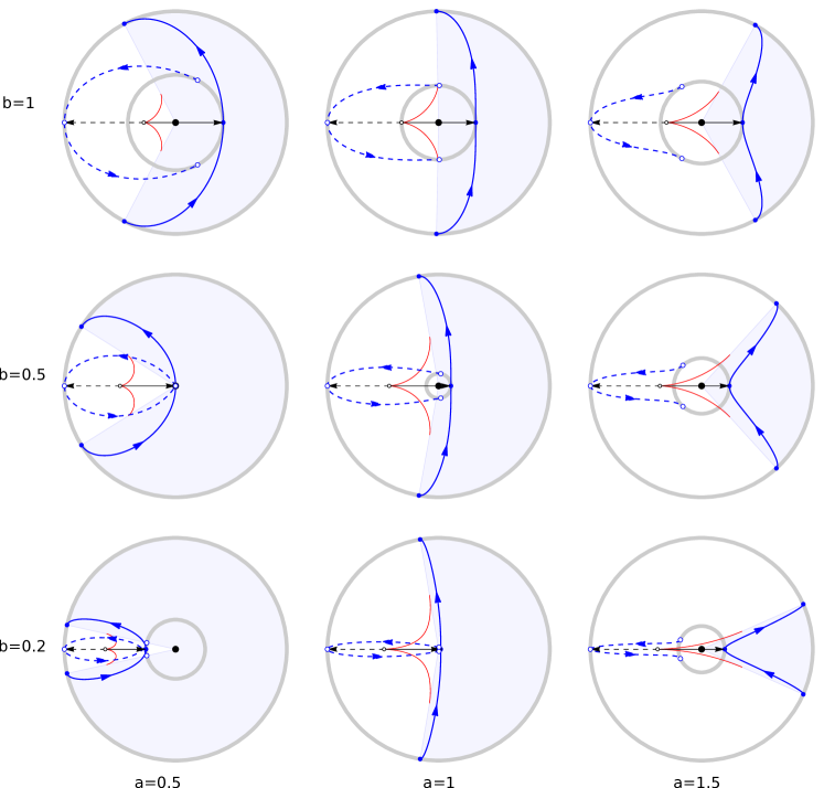
Figure 10: Numerical evidence supporting Conjecture 3.17. Bicycle correspondence of geodesics, projected onto ${\bf p}^{\perp}$, is shown for various values of the parameters $a,b$. The solid blue curve is ${\bf x}(t)$, the dashed curve is $\tilde{\bf x}(t)$, the red curve is their common back track ${\bf y}(t)$, all drawn in the range $0\leq t\leq T$, between two successive points of maximum distance of ${\bf x}(t)$ to the rotation axis. The rotation angle of the monodromy is marked by the darkened sector. Also marked is the bicycle correspondence between ${\bf x}(T/2)$ and $\tilde{\bf x}(T/2)$.

3.7 Global minimizers

Bicycle geodesics, by definition, have critical length among bicycle paths connecting two given placements of the bike frame. In particular, some of them are the minimizing bicycle paths. We shall not study them in detail but will only find the global minimizers, namely, the bike paths $({\bf x}(t),{\bf y}(t))$, $t\in{\mathbb{R}}$, which are minimizers for any of their finite subsegments.

There are two obvious candidates: those whose front tracks ${\bf x}(t)$ are straight lines or Euler’s solitons. Are there any other ones?

The answer is no. The reason is that, as we know, all other bicycle geodesics are quasi-periodic: ${\bf x}(t+T)=M({\bf x}(t))$, ${\bf y}(t+T)=M({\bf y}(t))$ for some $T>0$ and all $t$. Here is the detailed argument.

Proposition 3.18.

A quasi-periodic non-linear bicycle path is not a global minimizer.

Proof.

The argument is taken from [1, pages 4675-6], whose Figure 11 is reproduced here with minor changes as Figure 11.

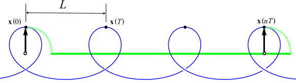
Figure 11: A shortcut.

Since ${\bf x}(t)$ is non-linear, there are two values of time, $T$ apart, say $0$ and $T$, so that the segment of ${\bf x}(t)$ between ${\bf x}(0)$ and ${\bf x}(T)$ is not a line segment. It follows that $L:=|{\bf x}(T)-{\bf x}(0)|<T$.

Now take the front track segment with end points at ${\bf x}(0),\ {\bf x}(nT)$ for some positive integer $n$. Its length is $nT$ and the distance between end points is at most $nL$.

Let the back track be ${\bf y}(t)$. Then $|{\bf y}(T)-{\bf y}(0)|\leq nL+2.$ So, for $n$ big enough, one can do better then $nT$ by

• reorienting the bike at $t=0$, with fixed back wheel, so it points to ${\bf y}(nT)$;

• ride straight towards ${\bf y}(nT)$;

• reorient the bike so its front wheel is at ${\bf x}(nT).$

Steps 1 and 3 cost at most some fixed amount independent of $n$, and step 2 costs at most $nL+2$. So total cost is at most $nL+c$, for some $c$ independent of $n$. This is less then $nT$ for $n$ big enough. ∎

Appendix A Explicit formulas

One can get explicit formulas for bicycling geodesics in ${\mathbb{R}}^{3}$ as a special case of those for Kirchhoff rods, as in [8, §4], but we found it actually easier to obtain them directly. (The formulas of [8] require first solving complicated algebraic equations for the parameters $p,w$ appearing in those formulas.) We use mostly the notation of [14].

Proposition A.1.

1. The curvature of a non-linear geodesic front track, parametrized by arc length, is given by

   $$\kappa^{2}(t)=(1+a)^{2}-4a\,{\rm sn}^{2}\left(\omega t,k\right)$$ (37)

   where

   $$\omega={\sqrt{(a+1)^{2}+b^{2}}\over 2},\qquad k^{2}={4a\over(a+1)^{2}+b^{2}}.$$ (38)

   Here ${\rm sn}(u,k)$ is the Jacobi elliptic function with modulus $k$ (or parameter $m=k^{2}$).

2. For $a\neq 1$ the period of the curvature $\kappa$ is the same as the period of $\kappa^{2}$, given by

   $$T={2K(k)\over\omega},$$

   where $K(k)$ is the complete elliptic integral of the first kind.

3. For $a=1$ (constant torsion front tracks) the front track’s curvature and its period are

   $$\kappa(t)=2{\rm cn}\left(\omega t,k\right),\quad 2T=\frac{4K(k)}{\omega}.$$

Proof.

As before, set $u:=\kappa^{2}$. Then $u(t)$ oscillates between the values $(1\pm a)^{2},$ satisfying equation (27),

$$\left({du\over dt}\right)^{2}=(u+b^{2})((1+a)^{2}-u)(u-(1-a)^{2}).$$

Making the change of variables $(t,u)\mapsto(x,y)$, where

$$u=(1+a)^{2}-4ay^{2},\quad x=\omega t,\quad\omega={\sqrt{(a+1)^{2}+b^{2}}\over 2},$$

one finds that $y(x)$ satisfies

$$\left(\frac{dy}{dx}\right)^{2}=(1-y^{2})(1-k^{2}y^{2}),$$

where

$$k^{2}={4a\over(a+1)^{2}+b^{2}}.$$

This is the ODE satisfied by the Jacobi elliptic function $y={\rm sn}(x,k)$, with $y(0)=0$ and period $4K(k)$, where $K(k)$ is the complete elliptic integral of the first kind with modulus $k$. Its square ${\rm sn}^{2}(x,k)$ has half that period, $2K(k)$. See formula 22.13.1 and Table 22.4.2 of [14]. ∎

Remark A.2.

Equation (37) of Proposition A.1 is the same as in [8, page 614], with $p^{2}=k^{2}$ given by equation (38) and

$$w^{2}={(1+a)^{2}\over(a+1)^{2}+b^{2}}.$$

The torsion of the front tracks of the last proposition is given by equation (25).

The curvature is periodic except for $a=1,b=0$, where one has $k=1$ and $K(1)=\infty$. In this case ${\bf x}(t)$ is the Euler soliton and one has

$$\kappa=2{\rm cn}(t,1)=2{\rm sech}(t).$$

We next give explicit formulas for the front tracks ${\bf x}(t)$ and their monodromy in cylindrical coordinates $r,\theta,z$ with respect to the rotation axis of ${\bf K}$.

Proposition A.3.

1. In cylindrical coordinates $r,\theta,z$ with respect to the rotation axis of ${\bf K}$, the front track of a bicycling geodesic, with initial conditions $z(0)=0$ and $\theta(0)=0$, is given by

   $$r(t) ={1\over|{\bf p}|}\sqrt{A-4a\,{\rm sn}^{2}(\omega t,k)},$$ (39)

   $$\theta(t) ={b\over 2|{\bf p}|}\left[t+{B\over\omega}\,\Pi(\omega t,n,k)\right],$$ (40)

   $$z(t) ={1\over 2|{\bf p}|}\left[(|{\bf p}|^{2}+1)t-4\omega\,E(\omega t,k)\right]$$ (41)

   where

   $$A=\frac{\left(|{\bf p}|^{2}+a\right)^{2}}{|{\bf p}|^{2}},\quad B=\frac{|{\bf p}|^{2}-a}{|{\bf p}|^{2}+a},\quad|{\bf p}|=\sqrt{a^{2}+b^{2}},\quad n=\frac{4a}{A},$$

   and $\omega,k$ are given in equation (38).

   Here $E(x,k),\Pi(x,n,k)$ are the incomplete elliptic integrals of the second and third kind, given by

   $$E(x,k):=x-k^{2}\int_{0}^{x}{\rm sn}^{2}(s,k)ds,$$ (42)

   $$\Pi(x,n,k):=\int_{0}^{x}{ds\over 1-n\,{\rm sn}^{2}(s,k)}.$$ (43)

2. The monodromy is given by

   $$\Delta\theta ={b\over\omega|{\bf p}|}\left[K(k)+B\,\Pi(n,k)\right],$$ (44)

   $$\Delta z ={1\over\omega|{\bf p}|}\left[(|{\bf p}|^{2}+1)K(k)-4\omega^{2}E(k)\right],$$ (45)

   where $K(k),\ E(k):=E(K(k),k)$ and $\Pi(n,k):=\Pi(K(k),n,k)$ are the complete elliptic integrals of the first, second, and third kinds, respectively.

Proof.

From the proof of Proposition 3.12 we have equation (35),

$$b^{2}+\kappa^{2}=|{\bf p}|^{2}r^{2}+{b^{2}\over|{\bf p}|^{2}},$$ (46)

from which one obtains equation (39) using equation (37) and $|{\bf p}|=\sqrt{a^{2}+b^{2}}$.

Next, from equation (21), $2|{\bf p}|z^{\prime}=1+a^{2}-\kappa^{2},$ and upon substitution of equation (37), we have

$$|{\bf p}|z^{\prime}=a\left[2{\rm sn}^{2}(\omega t,k)-1\right].$$ (47)

Equation (41) follows by using formula (42).

Dotting both sides of (23) with ${\bf x}^{\prime}$ and using the expression for ${\bf K}$ from (14), one obtains

$$r^{2}|{\bf p}|\,\theta^{\prime}=b\left(1-\frac{z^{\prime}}{|{\bf p}|}\right),$$

from which, upon substitution of the above formulas (47) for $z^{\prime}$ and (46) for $r$, we find

$$|{\bf p}|\theta^{\prime}=\frac{b}{2}\left[1+\left(\frac{2(|{\bf p}|^{2}+a)}{A}-1\right)\frac{1}{1-n\,{\rm sn}^{2}(\omega t,k)}\right],\mbox{ where }n:=\frac{4a}{A}.$$

Equation (40) now follows from formula (43).

Equations (45)-(44) now follow by evaluating equations (40)-(41) at $t=T=2K/\omega$, and using $E(2K(k),k)=2E(k),$ $\Pi(2K(k),n,k)=2\Pi(n,k).$ ∎

Remark A.4.

The explicit formulas (39)-(41) are given for general Kirchoff rods in [16], where they appear as equations (4.19a)-(4.19c).

References

- [1] A. Ardentov, G. Bor, E. Le Donne, R. Montgomery, Yu. Sachkov. Bicycle paths, elasticae and sub-Riemannian geometry. Nonlinearity 34 (2021), 4661–4683.
- [2] G. Bor, M. Levi, R. Perline, S. Tabachnikov. Tire track geometry and integrable curve evolution. Int. Math. Res. Notices, 2020, no. 9, 2698–2768.
- [3] M. Barrosa, J. Cabrerizo, M. Fernández, A. Romero. Magnetic vortex filament flows. J. Math. Phys. 48.8 (2007), 082904.
- [4] S. Dru\textcommabelowt-Romaniuc, M. Munteanu. Magnetic curves corresponding to Killing magnetic fields in . J. Math. Phys. 52.11 (2011), 113506.
- [5] R. Foote, M. Levi, S. Tabachnikov, Serge. Tractrices, bicycle tire tracks, hatchet planimeters, and a 100-year-old conjecture. Amer. Math. Monthly 120 (2013), 199–216.
- [6] W.C. Graustein. Differential geometry. The Macmillan Company, New York (1935).
- [7] G. Kirchhoff. On the balance and motion of an infinitely thin elastic rod. J. Pure App. Math. (Crelles Journal) 56 (1859), 285–313.
- [8] J. Langer, D. Singer. Lagrangian aspects of the Kirchhoff elastic rod. SIAM Rev. 38 (1996), 605–618.
- [9] J. Langer. Recursion in curve geometry. New York J. Math. 5 (1999), 25–51.
- [10] R. Montgomery. A Tour of SubRiemannian Geometry. Amer. Math. Soc., Providence, RI (2006).
- [11] M. Munteanu. Magnetic curves in a euclidean space:one example, several approaches. Publ. Inst. Math. (Beograd) (N.S.) 94.108 (2013), 141–150.
- [12] K. Nomizu. On Frenet equations for curves of class . Tohoku Math. J. 11.1 (1959), 106–112.
- [13] O. M. O’Reilly. Modeling Nonlinear Problems in the Mechanics of Strings and Rods. Springer, Cham (2017).
- [14] P. Reinhardt, P. L. Walker. Jacobian Elliptic Functions. Chap. 22 of NIST Handbook Math. Functions, Cambridge Univ. Press, Cambridge, 2010. https://dlmf.nist.gov/22.
- [15] C. Rogers, W. Schief. Bäcklund and Darboux Transformations. Cambridge Univ. Press, Cambridge, 2002.
- [16] Y. Shi, J.E. Hearst. The Kirchhoff elastic rod, the nonlinear Schrdinger equation, and DNA supercoiling. J. of Chem. Phys. 101.6 (1994), 5186–5200.
- [17] D. Singer. Lectures on elastic curves and rods. Curvature and variational modeling in physics and biophysics, 3–32, AIP Conf. Proc., 1002, Amer. Inst. Phys., Melville, NY, 2008.
- [18] S. Tabachnikov. On the bicycle transformation and the filament equation: Results and conjectures. J. Geom. Phys. 115 (2017), 116–123.