Abstract

We reanalyze in a simple and comprehensive manner the recently released SH0ES data for the determination of $H_{0}$. We focus on testing the homogeneity of the Cepheid+SnIa sample and the robustness of the results in the presence of new degrees of freedom in the modeling of Cepheids and SnIa. We thus focus on the four modeling parameters of the analysis: the fiducial luminosity of SnIa $M_{B}$ and Cepheids $M_{W}$ and the two parameters ($b_{W}$ and $Z_{W}$) standardizing Cepheid luminosities with period and metallicity. After reproducing the SH0ES baseline model results, we allow for a transition of the value of any one of these parameters at a given distance $D_{c}$ or cosmic time $t_{c}$ thus adding a single degree of freedom in the analysis. When the SnIa absolute magnitude $M_{B}$ is allowed to have a transition at $D_{c}\simeq 50Mpc$ (about $160Myrs$ ago), the best fit value of the Hubble parameter drops from $H_{0}=73.04\pm 1.04\,km\,s^{-1}\,Mpc^{-1}$ to $H_{0}=67.32\pm 4.64\,km\,s^{-1}\,Mpc^{-1}$ in full consistency with the Planck value. Also, the best fit SnIa absolute magnitude $M_{B}^{>}$ for $D>D_{c}$ drops to the Planck inverse distance ladder value $M_{B}^{>}=-19.43\pm 0.15$ while the low distance best fit $M_{B}^{<}$ parameter remains close to the original distance ladder calibrated value $M_{B}^{<}=-19.25\pm 0.03$. Similar hints for a transition behavior is found for the other three main parameters of the analysis ($b_{W}$, $M_{W}$ and $Z_{W}$) at the same critical distance $D_{c}\simeq 50\,Mpc$ even though in that case the best fit value of $H_{0}$ is not significantly affected. When the inverse distance ladder constraint on $M_{B}^{>}$ is included in the analysis, the uncertainties for $H_{0}$ reduce dramatically ($H_{0}=68.2\pm 0.8\,km\,s^{-1}\,Mpc^{-1}$) and the $M_{B}$ transition model is strongly preferred over the baseline SH0ES model ($\Delta\chi^{2}\simeq-15$, $\Delta AIC\simeq-13$) according to AIC and BIC model selection criteria.

1 1 0 Academic Editor: Firstname Lastname https://doi.org/ A reanalysis of the latest SH0ES data for $H_{0}$:
Effects of new degrees of freedom on the Hubble tension. title Leandros Perivolaropoulos^1,† and Foteini Skara^1,‡ Leandros Perivolaropoulos, Foteini Skara Perivolaropoulos, L.;Skara, F. leandros@uoi.gr f.skara@uoi.gr

1 Introduction

1.1 The current status of the Hubble tension and its four assumptions

Measurements of the Hubble constant using observations of type Ia supernovae (SnIa) with Cepheid calibrators by the SH0ES Team has lead to a best fit value $H_{0}^{R21}=73.04\pm 1.04$ km s^-1 Mpc^-1 Riess et al. (2022) (hereafter R21). This highly precise but not necessarily accurate measurement is consistent with a wide range of other less precise local measurements of $H_{0}$ using alternative SnIa calibrators Freedman (2021); Gómez-Valent and Amendola (2018); Pesce et al. (2020); Freedman et al. (2020), gravitational lensing Wong et al. (2020); Chen et al. (2019); Birrer et al. (2020, 2019), gravitational waves Fishbach et al. (2019); Hotokezaka et al. (2019); Abbott et al. (2017); Palmese et al. (2020); Soares-Santos et al. (2019), gamma-ray bursts as standardizable candles Cao et al. (2022a, b); Dainotti et al. (2022a, b, 2013), quasars as distant standard candles Risaliti and Lusso (2019), type II supernovae de Jaeger et al. (2022, 2020), $\gamma-$ray attenuation Domínguez et al. (2019) etc. (for recent reviews see Refs. Di Valentino et al. (2021); Perivolaropoulos and Skara (2022)). This measurement is based on two simple assumptions:

• There are no significant systematic errors in the measurements of the properties (period, metallicity) and luminosities of Cepheid calibrators and SnIa.

• The physical laws involved and the calibration properties of Cepheids and SnIa in all the rungs of the distance ladder are well understood and modelled properly.

This measurement however is at $5\sigma$ tension (Hubble tension) with the corresponding measurement from Planck observations of the CMB angular power spectrum (early time inverse distance ladder measurement) $H_{0}^{P18}=67.36\pm 0.54$ km s^-1 Mpc^-1 Aghanim et al. (2020) (see also Refs. Perivolaropoulos and Skara (2022); Abdalla et al. (2022); Di Valentino et al. (2021); Shah et al. (2021); Knox and Millea (2019); Vagnozzi (2020); Ishak (2019); Mörtsell and Dhawan (2018); Huterer and Shafer (2018); Bernal et al. (2016) for relevant recent reviews). This inverse distance ladder measurement is also based on two basic assumptions:

• The scale of the sound horizon at the last scattering surface is the one calculated in the context of the standard cosmological model with the known degrees of freedom (cold dark matter, baryons and radiation) and thus it is a reliable distance calibrator.

• The evolution of the Hubble free expansion rate $E(z)\equiv H(z)/H_{0}$ from the time of recombination (redshift $z=z_{rec}$) until the present time ($z=0$) is the one predicted by the standard $\Lambda$CDM model as defined by the best fit Planck parameters (Planck18$/\Lambda$CDM) Aghanim et al. (2020); Alam et al. (2021).

A wide range of approaches have been implemented in efforts to explain this Hubble tension (for reviews see Refs. Bernal et al. (2016); Perivolaropoulos and Skara (2022); Verde et al. (2019); Di Valentino et al. (2021); Schöneberg et al. (2021); Abdalla et al. (2022); Krishnan et al. (2020); Jedamzik et al. (2020)). These approaches introduce new degrees of freedom that violate at least one of the above four assumptions and may be classified in accordance with the particular assumption they are designed to violate.

Thus, early time sound horizon models introduce new degrees of freedom at the time just before recombination (e.g. early dark energy Poulin et al. (2019); Niedermann and Sloth (2021); Verde et al. (2019); Smith et al. (2022, 2020); Chudaykin et al. (2020); Fondi et al. (2022); Sabla and Caldwell (2022); Herold et al. (2022); McDonough et al. (2022); Hill et al. (2020); Sakstein and Trodden (2020); Niedermann and Sloth (2020); Rezazadeh et al. (2022), radiation Green et al. (2019); Schöneberg and Franco Abellán (2022); Seto and Toda (2021); Carrillo González et al. (2020) or modified gravity Braglia et al. (2021); Abadi and Kovetz (2021); Renk et al. (2017); Nojiri et al. (2022); Lin et al. (2019); Saridakis et al. (2021)) to change the expansion rate at that time and thus decrease the sound horizon scale $r_{s}$ (early time distance calibrator) to increase $H_{0}$, which is degenerate with $r_{s}$, to a value consistent with local measurements.

The mechanism proposed by these models attempts to decrease the scale of the sound horizon at recombination which can be calculated as

$$r_{s}=\int_{0}^{t_{*}}\frac{c_{s}(a)}{a(t)}dt=\int_{z_{*}}^{\infty}\frac{c_{s}(z)}{H(z;\rho_{b},\rho_{\gamma},\rho_{c})}dz=\int_{0}^{a_{*}}\frac{c_{s}(a)}{a^{2}H(a;\rho_{b},\rho_{\gamma},\rho_{c})}da$$ (1)

where the recombination redshift $z_{*}$ corresponds to time $t_{*}$, $\rho_{b}$, $\rho_{c}$ and $\rho_{\gamma}$ denote the densities for baryon, cold dark matter and radiation (photons) respectively and $c_{s}$ is the sound speed in the photon-baryon fluid. The angular scale of the sound horizon is measured by the peak locations of the CMB perturbations angular power spectrum and may be expressed in terms of $r_{s}$ as

$$\theta_{s}=\frac{r_{s}}{d_{A}}=\frac{H_{0}r_{s}}{c\int_{0}^{z_{*}}\frac{dz^{\prime}}{E(z^{\prime})}}$$ (2)

where $d_{A}$ is the comoving angular diameter distance to last scattering (at redshift $z\approx 1100$) and $E(z)$ is the dimensionless normalized Hubble parameter which for a flat $\Lambda$CDM model is given by

$$E(z)\equiv\frac{H(z)}{H_{0}}=\left[\Omega_{0m}(1+z)^{3}+(1-\Omega_{0m})\right]^{1/2}$$ (3)

Eq. (2) indicates that there is a degeneracy between $r_{s}$, $H_{0}$ and $E(z)$ given the measured value of $\theta_{s}$. A decrease of $r_{s}$ would lead to an increase of the predicted value of $H_{0}$ (early time models) and a late time deformation of $E(z)$ could lead to an increase of the denominator of Eq. (2) leading also to an increase of $H_{0}$ (late time models).

Early dark energy models have the problem of predicting stronger growth of perturbations than implied by dynamical probes like redshift space distortion (RSD) and weak lensing (WL) data and thus may worsen the $\Omega_{m}$-$\sigma_{8}$ growth tension Benisty (2021); Heymans et al. (2021); Kazantzidis and Perivolaropoulos (2018); Joudaki et al. (2018); Kazantzidis and Perivolaropoulos (2019); Skara and Perivolaropoulos (2020); Avila et al. (2022); Köhlinger et al. (2017); Nunes and Vagnozzi (2021); Clark et al. (2021) and reduce consistency with growth data and with other cosmological probes and conjectures Ivanov et al. (2020); Hill et al. (2022, 2020); Clark et al. (2021); Jedamzik et al. (2020); Herold et al. (2022); Vagnozzi (2021); Krishnan et al. (2020); Philcox et al. (2022); McDonough et al. (2022). Thus, a compelling and full resolution of the Hubble tension may require multiple (or other) modifications beyond the scale of the sound horizon predicted by $\Lambda$CDM cosmology. Even though these models are severely constrained by various cosmological observables, they currently constitute the most widely studied class of models Smith et al. (2020); Chudaykin et al. (2021); Sakstein and Trodden (2020); Reeves et al. (2022); Chudaykin et al. (2020); Smith et al. (2022).

Late time $H(z)$ deformation models introduce new degrees of freedom (e.g. modified gravity Solà Peracaula et al. (2020); Braglia et al. (2020); Pogosian et al. (2021); Bahamonde et al. (2021) dynamical late dark energy Di Valentino et al. (2021); Alestas et al. (2020); Di Valentino et al. (2020); Pan et al. (2020); Li and Shafieloo (2019); Zhao et al. (2017); Keeley et al. (2019); Sola Peracaula et al. (2019); Yang et al. (2019); Krishnan et al. (2021); Dainotti et al. (2021); Colgáin et al. (2022a, b); Zhou et al. (2021) or interacting dark energy with matter Di Valentino et al. (2020); Yang et al. (2018); Vattis et al. (2019); Di Valentino et al. (2020); Yang et al. (2018); Ghosh et al. (2020)) to deform $E(z)$ at redshifts $z\sim O(1)$ so that the present time value of $H(z=0)=H_{0}$ increases and becomes consistent with the local measurements. This class of models is even more severely constrained Brieden et al. (2022); Alestas et al. (2020); Alestas and Perivolaropoulos (2021); Keeley and Shafieloo (2022); Clark et al. (2020); Chen et al. (2021); Anchordoqui et al. (2022); Mau et al. (2022); Cai et al. (2022); Heisenberg et al. (2022); Vagnozzi et al. (2022); Davari and Khosravi (2022), by other cosmological observables (SnIa, BAO and growth of perturbations probes) which tightly constrain any deformation Alam et al. (2021) from the Planck18/$\Lambda$CDM shape of $E(z)\equiv H(z)/H_{0}$.

The third approach to the resolution of the Hubble tension is based on a search for possible unaccounted systematic effects including possible issues in modelling the Cepheid data such as non-standard dust induced color correction Mortsell et al. (2021), the impact of outliers Efstathiou (2014, 2020, 2021), blending effects, SnIa color properties Wojtak and Hjorth (2022), robustness of the constancy of the SnIa absolute magnitude in the Hubble flow Benisty et al. (2022); Martinelli and Tutusaus (2019); Tinsley (1968); Kang et al. (2020); Rose et al. (2019); Jones et al. (2018); Rigault et al. (2020); Kim et al. (2018); Colgáin (2019); Kazantzidis and Perivolaropoulos (2019, 2020); Sapone et al. (2021); Koo et al. (2020); Kazantzidis et al. (2021); Luković et al. (2020); Tutusaus et al. (2019, 2017); Drell et al. (2000) etc. There is currently a debate about the importance of these potential systematic effects Kenworthy et al. (2019); Riess et al. (2022); Yuan et al. (2022); Riess et al. (2018). Also the possibility for redshift evolution of Hubble constant was studied by Ref. Dainotti et al. (2022). In Dainotti et al. (2022) the Hubble tension has been analyzed with a binned analysis on the Pantheon sample of SNe Ia through a multidimensional MCMC analysis. Finally the need for new standardizable candles with redshift values far beyond the SnIa ($3\lesssim z\lesssim 9$) has been studied (see Refs. Cao et al. (2022a, b); Dainotti et al. (2022a, b, 2013) for gamma-ray bursts and Refs. Bargiacchi et al. (2021); Dainotti et al. (2022) for quasars).

A fourth approach related to the previous one is based on a possible change of the physical laws (e.g. a gravitational transitionKhosravi and Farhang (2022); Perivolaropoulos and Skara (2022)) during the past $200\,Myrs$ ($z\lesssim 0.01$) when the light of the Cepheid calibrator hosts was emitted Alestas et al. (2022); Desmond et al. (2019); Perivolaropoulos and Skara (2021); Odintsov and Oikonomou (2022); Alestas et al. (2021); Marra and Perivolaropoulos (2021); Alestas et al. (2021); Perivolaropoulos (2022); Perivolaropoulos and Skara (2022); Odintsov and Oikonomou (2022). In this context, new degrees of freedom should be allowed for the modeling of either Cepheid calibrators or/and SnIa to allow for the possibility of this physics change. If these degrees of freedom are shown not to be excited by the data then this approach would also be severely constrained. It is possible however that nontrivial values of these new parameters are favored by the data while at the same time the best fit value of $H_{0}$ shifts to a value consistent with the inverse distance ladder measurements of $H_{0}$ using the sound horizon at recombination as calibrator. In this case Perivolaropoulos and Skara (2021), this class of models would be favored especially in view of the severe constraints that have been imposed on the other three approaches.

The possible new degrees of freedom that could be allowed in the Cepheid+SnIa modeling analysis are clearly infinite but the actual choices to be implemented in a generalized analysis may be guided by three principles: simplicity, physical motivation and improvement of the quality of fit to the data.

In a recent analysis Perivolaropoulos and Skara (2021) using a previous release of the SH0ES data Riess et al. (2016, 2019, 2021) we showed that a physically motivated new degree of freedom in the Cepheid calibrator analysis allowing for a transition in one of the Cepheid modelling parameters $R_{W}$ or $M_{W}$, is mildly favored by the data and can lead to a reduced best fit value of $H_{0}$. Here we extend that analysis in a detailed and comprehensive manner, to a wider range of transition degrees of freedom using the latest publicly available SH0ES data described in R21.

1.2 The new SH0ES Cepheid+SnIa data

Table 1: A comparison of the latest SH0ES data release (R21) with previous data updates.

SH0ES	Cepheid + SnIa	Cepheids	Calibrator	Hubble flow
Year/Ref.	host galaxies		SnIa	SnIa
		MW    15
		LMCa   785
2016	19	N4258   139	19	217
R16 Riess et al. (2016)	$z<0.01$	M31     372	$z<0.01$	$0.0233<z<0.15$
		Total   1311
		In SnIa hosts   975
		Total All  2286
		MW    15
		LMCb   785+70
2019	19	N4258    139	19	217
R19 Riess et al. (2019)	$z<0.01$	M31     372	$z<0.01$	$0.0233<z<0.15$
		Total   1381
		In SnIa hosts   975
		Total All  2356
		MW    75
		LMCb   785+70
2020	19	N4258   139	19	217
R20 Riess et al. (2021)	$z<0.01$	M31     372	$z<0.01$	$0.0233<z<0.15$
		Total   1441
		In SnIa hosts   975
		Total All   2416
		LMCb   270+69
		SMCa   143
2021	37	N4258   443	42	277
R21 Riess et al. (2022)	$0.0015\lesssim z<0.011$	M31        55	$0.0015\lesssim z<0.011$	$0.023<z<0.15$
		Total      980
		In SnIa hosts  2150	(77 lightcurve meas.)
		Total All  3130

NOTE - (a) From the ground. (b) From the ground+HST.

The new Cepheid+SnIa data release and analysis from the SH0ES collaboration in R21 includes a significant increase of the sample of SnIa calibrators from 19 in Ref. Riess et al. (2016) to 42. These SnIa reside in 37 hosts observed between 1980 and 2021 in a redshift range $0.0015\lesssim z<0.011$ (see Table 1 for a more detailed comparison of the latest SH0ES data release with previous updates). These SnIa are calibrated using Cepheids in the SnIa host galaxies. In turn, Cepheid luminosities are calibrated using geometric methods in calibrator nearby galaxies (anchors). These anchor galaxies include the megamaser host NGC 4258, the Milky Way (MW) where distances are measured with several parallaxes, and the Large Magellanic Cloud (LMC) where distances are measured via detached eclipsing binaries Riess et al. (2019) as well as two supporting anchor galaxies ($M31$ Li et al. (2021) and the Small Magellanic Cloud (SMC). These supporting galaxies are pure Cepheid hosts and do not host SnIa but host large and well measured Cepheid samples. However, geometric measurements of their distances are not so reliable and thus are not directly used in the analysis. The calibrated SnIa in the Hubble flow ($z\gtrsim 0.01$) are used to measure $H_{0}$ due to to their high precision (5% in distance per source) and high luminosity which allows deep reach and thus reduces the impact of local velocity flows.

The new SH0ES data release includes a factor of 3 increase in the sample of Cepheids within NGC 4258. In total it has 2150 Cepheids in SnIa hosts, 980 Cepheids in anchors or supporting galaxies, 42 SnIa (with total 77 lightcurve dataset measurements) in 37 Cepheid+SnIa hosts with redshifts $0.0015\lesssim z<0.011$ and 277 SnIa in the Hubble flow in the redshift range $0.023<z<0.15$. In addition 8 anchor based constraints (with uncertainties included) constrain the following Cepheid modeling parameters: $M_{W}$ (the Cepheid absolute magnitude zeropoint), $b_{W}$ (the slope of the Cepheid Period-Luminosity P-L relation), $Z_{W}$ (the slope of the Cepheid Metallicity-Luminosity M-L relation), a zeropoint parameter $zp$ used to refine the Cepheid P-L relation by describing the difference between the ground and HST zeropoints in LMC Cepheids (zp is set to 0 for HST observations), the distance moduli of the anchors NGC 4258 and LMC and a dummy parameter we call $X$ which has been included in the R21 data release and is set to 0 with uncertainty $10^{-9}$ .

The parameters fit with these data include the four modeling parameters $M_{W}$, $b_{W}$, $Z_{W}$, $M_{B}$ (the SnIa absolute magnitude), the 37 distance moduli of SnIa/Cepheid hosts, the distance moduli to the 2 anchors (NGC 4258, LMC) and to the supporting Cepheid host M31, the zeropoint $zp$ of the Cepheid P-L relation in the LMC ground observations, the Hubble parameter and the dummy parameter mentioned above (tightly constrained to 0). This is a total of 47 parameters (46 if the dummy parameter $X$ is ignored).

In addition to these parameters, there are other modeling parameters like the color and shape correction slopes of SnIa (usually denoted as $\beta$ and $\alpha$) as well as the Wesenheit dust extinction parameter $R_{W}$ which have been incorporated in the released SnIa and Cepheid apparent magnitudes and thus can not be used as independent parameters in the analysis, in contrast to the previous data release.

The provided in R21 Cepheid Wesenheit dust corrected dereddened apparent magnitudes $m_{H}^{W}$ are connected with the Wesenheit dust extinction parameter $R_{W}$ as Madore (1982) (see also Refs. Riess et al. (2016, 2019))

$$m_{H}^{W}\equiv m_{H}-R_{W}(V-I)$$ (4)

where $m_{H}$ is the observed apparent magnitude in the near-infrared $H$ (F160W) band, $V$ (F555W) and $I$ (F814W) are optical mean apparent magnitudes in the corresponding bands. The empirical parameter $R_{W}$ is also called ’the reddening-free "Wesenheit" color ratio’ and is different from $R_{H}$ which can be derived from a dust law (e.g. the Fitzpatrick law Fitzpatrick (1999)). The parameter $R_{W}$ corrects for both dust and intrinsic variations applied to observed blackbody colors $V-I$.

The provided in R21 SnIa apparent magnitudes $m_{B}^{0}$, standardized using light curve color c and shape $x_{1}$ corrections are defined as

$$m_{B}^{0}\equiv m_{B}-\alpha\;x_{1}-\beta\;c=\mu+M_{B}$$ (5)

where $m_{B}$ is the peak apparent magnitude, $\mu$ is the SnIa distance modulus while the B-band absolute magnitude, $M_{B}$, and correction coefficients $\alpha$ and $\beta$ are fit directly using the SnIa data. The latest SH0ES data release provides the measured values of $m_{H}^{W}$ and $m_{B}^{0}$ for Cepheid and SnIa respectively which are also used in the corresponding analysis while the parameters $R_{W}$, $\alpha$ and $\beta$ are fit previously and independently by the SH0ES team to provide the values of $m_{H}^{W}$ and $m_{B}^{0}$.

1.3 The prospect of new degrees of freedom in the SH0ES data analysis

The homogeneity of the SH0ES data with respect to the parameters $R_{W}$, $\alpha$ and $\beta$ has been analysed in previous studies with some interesting results. In particular, using the data of the previous SH0ES data release Riess et al. (2016, 2019, 2021), it was shown Perivolaropoulos and Skara (2021) (see also Mortsell et al. (2021) for a relevant study) that if the parameter $R_{W}$ is allowed to vary among Cepheid and SnIa hosts then the fit quality is significantly improved and the best fit value of $H_{0}$ is lowered to a level consistent with the inverse distance ladder best fit. In addition, a more recent analysis has allowed the parameter $\beta$ to have a different value in Hubble flow SnIa ($\beta=\beta_{HF}$ for $z>0.02$) compared to calibrating SnIa ($\beta=\beta_{cal}$ for $z<0.01$). A reanalysis allowing for this new degree of freedom has indicated a tension between the the two best fit values ($\beta_{HF}$ and $\beta_{cal}$) at a level of up to $3.8\sigma$ Wojtak and Hjorth (2022).

Motivated by these hints for inhomogeneities in the SH0ES data, in what follows we introduce new degrees of freedom in the analysis that are designed to probe the origin of these inhomogeneities. We thus accept three of the four above mentioned assumptions that have lead to the Hubble tension and test the validity of the fourth assumption. In particular we keep the following assumptions:

1. There are no significant systematics in the SH0ES data and thus they are reliable.

2. The CMB sound horizon scale used as a calibrator in the inverse distance ladder approach is correctly obtained in the standard model using the known particles.

3. The Hubble expansion history from the time of recombination up to $z=0.01$ (or even $z=0$) used in the inverse distance ladder measurement of $H_{0}$ is provided correctly by the standard Planck18$/\Lambda$CDM cosmological model.

As discussed above there are several studies in the literature that support the validity of these assumptions (e.g. Fondi et al. (2022); Keeley and Shafieloo (2022)). If these assumptions are valid then the most probable source of the Hubble tension is the violation of the fourth assumption stated above namely ’the physical laws involved and the calibration properties of Cepheids and SnIa in all the rungs of the distance ladder are well understood and modelled properly’.

If this assumption is violated then the modeling of Cepheids+SnIa should be modified to take into account possible changes of physics by introducing new degrees of freedom that were suppressed in the original (baseline) SH0ES analysis. In the context of this approach, if these degrees of freedom are properly introduced in the analysis then the best fit value of $H_{0}$ will become consistent with the corresponding inverse distance ladder value of $H_{0}=67.36\pm 0.54$ km s^-1 Mpc^-1.

In an effort to pursue this approach for the resolution of the Hubble tension we address the following questions:

• How can new degrees of freedom (new parameters) be included in the SH0ES data analysis for the determination of $H_{0}$?

• What are the new degrees of freedom that can expose internal tensions and inhomogeneities in the Cepheid/SnIa data?

• What new degrees of freedom can lead to a best fit value of $H_{0}$ that is consistent with Planck?

The main goal of the present analysis is to address these questions. The new degree of freedom we allow and investigate is a transition of any one of the four Cepheid/SnIa modeling parameters at a specific distance $D_{c}$ or equivalently (in the context of the cosmological principle) at a given cosmic time $t_{c}$ such that $t_{0}-t_{c}=D_{c}/c$ where $t_{0}$ is the present cosmic time (age of the Universe). In the context of this new degree of freedom we reanalyse the SH0ES data to find how does the quality of fit to the data and the best fit value of $H_{0}$ change when the new degree of freedom is excited. The possible introduction of new constraints included in the analysis is also considered.

The structure of this paper is the following: In the next section 2 we describe the standard analysis of the SH0ES Cepheid+SnIa data in a detailed and comprehensive manner stressing some details of the released dataset that are not described in R21. We also describe some tension between the values of the best fit Cepheid modeling parameters $b_{W}$ and $Z_{W}$ obtained in anchor or pure Cepheid host galaxies and the corresponding mean values obtained in SnIa host galaxies. In section 3 we present our generalized analysis with new degrees of freedom that allow a transition of the main modeling parameters at specific distances (cosmic times of radiation emission). We also investigate the effect of the inverse distance ladder constraint on $M_{B}$ Camarena and Marra (2021); Marra and Perivolaropoulos (2021); Gómez-Valent (2022) for both the baseline SH0ES analysis and for our analysis involving the $M_{B}$ transition degree of freedom. Finally in section 4 we conclude, discuss the implications of our results and the possible extensions of our analysis.

2 The new SH0ES data and their standard analysis: Hints for intrinsic tensions

2.1 The original baseline SH0ES analysis: a comprehensive presentation

The main equations used to model the Cepheid SnIa measured apparent magnitudes with parameters that include $H_{0}$ are described as follows:

• The equation that connects the measured Wesenheit magnitude of the $j$th Cepheid in the $i$th galaxy, with the host distance moduli $\mu_{i}$ and the modeling parameters $M_{W}$, $b_{W}$ and $Z_{W}$ is of the form

  $$m_{H,i,j}^{W}=\mu_{i}+M_{H}^{W}+b_{W}[P]_{i,j}+Z_{W}[O/H]_{i,j}$$ (6)

  where $\mu_{i}$ is the inferred distance modulus to the galaxy, $M_{H}^{W}$ is the zeropoint Cepheid absolute magnitude of a period $P=10\,d$ Cepheid ($d$ for days), and $b_{W}$-$Z_{W}$ are the slope parameters that represent the dependence of magnitude on both period and metallicity. The $[O/H]$ is a measure of the metallicity of the Cepheid. The usual bracket shorthand notation for the metallicity $[O/H]$ represents the Cepheid metal abundance compared to that of the Sun

  $$[O/H]\equiv\log(O/H)-\log(O/H)_{\odot}=\Delta\log(O/H)$$ (7)

  Here O and H is the number of oxygen and hydrogen atoms per unit of volume respectively. The unit often used for metallicity is the dex (decimal exponent) defined as $n\,dex\equiv 10^{n}$. Also, the bracket shorthand notation for the period $[P]$ is used as ($P$ in units of days)

  $$[P]\equiv\log P-1$$ (8)

• The color and shape corrected SnIa B-band peak magnitude in the $i$th host is connected with the distance modulus $\mu_{i}$ of the $i$th host and with the SnIa absolute magnitude $M_{B}$ as shown in Eq. (5) i.e.

  $$m_{B,i}^{0}=\mu_{i}+M_{B}$$ (9)

  The distance modulus is connected with the luminosity distance $d_{L}$ in $Mpc$ as

  $$\mu=5\log(d_{L}/Mpc)+25$$ (10)

  where in a flat universe

  $$d_{L}(z)=c(1+z)\int_{0}^{z}\frac{dz^{\prime}}{H(z^{\prime})}=cH_{0}^{-1}(1+z)\int_{0}^{z}\frac{H_{0}\;dz^{\prime}}{H(z^{\prime})}\equiv H_{0}^{-1}\;D_{L}(z)$$ (11)

  where $D_{L}(z)$ is the Hubble free luminosity distance which is independent of $H_{0}$.

• Using Eqs. (9)-(11) it is easy to show that that $H_{0}$ is connected with the SnIa absolute magnitude and the Hubble free luminosity distance as

  $$5\log H_{0}=M_{B}+5\log D_{L}(z)-m_{B}^{0}(z)+25$$ (12)

  In the context of a cosmographic expansion of $H(z)$ valid for $z<<1$ we have

  $$\log D_{L}(z)_{c}\simeq\log\left[cz\left(1+\frac{1}{2}(1-q_{0})z-\frac{1}{6}(1-q_{0}-3q_{0}^{2}+j_{0})z^{2}+\mathcal{O}(z^{3})\right)\right]$$ (13)

  where $q_{0}\equiv-\frac{1}{H_{0}^{2}}\frac{d^{2}a(t)}{dt^{2}}\Big{|}_{t=t_{0}}$ and $j_{0}\equiv\frac{1}{H_{0}^{3}}\frac{d^{3}a(t)}{dt^{3}}\Big{|}_{t=t_{0}}$ are the deceleration and jerk parameters respectively. Thus Eqs. (12) and (13) lead to the equation that connects $H_{0}$ with the SnIa absolute magnitude $M_{B}$ which may be expressed as

  $$5\log H_{0}=M_{B}+5\log D_{L}(z)-m_{B}^{0}(z)+25\equiv M_{B}+5\;a_{B}+25$$ (14)

  where we have introduced the parameter $a_{B}\equiv\log D_{L}(z)-0.2m_{B}^{0}(z)$ as defined in the SH0ES analysis Riess et al. (2016).

Thus the basic modeling equations used in the SH0ES analysis for the measurement of $H_{0}$ are Eqs. (6), (9) and (14). In these equations the input data are the measured apparent magnitudes (luminosities) of Cepheids $m_{H,i,j}^{W}$ and the SnIa apparent magnitudes $m_{B,i}^{0}$ (in Cepheid+SnIa hosts and in the Hubble flow). The parameters to be fit using a maximum likelihood method are the distance moduli $\mu_{i}$ (of the anchors and supporting hosts, the Cepheid+SnIa hosts and Hubble flow SnIa), the four modeling parameters ($M_{H}^{W}$, $b_{W}$, $Z_{W}$ and $M_{B}$), the Hubble constant $H_{0}$, the zeropoint $zp$ of the Cepheid P-L relation in the LMC ground measurements and the dummy parameter $X$. This is a total of 47 parameters. The actual data have been released by the SH0ES team as a .fits file in the form of a column vector $Y$ with 3492 entries which includes 8 constraints on the parameters obtained from measurements in anchor galaxies where the distance moduli are measured directly with geometric methods.

The entries of the provided $Y$ data column vector do not include the pure measured apparent magnitudes. Instead its entries are residuals defined by subtracting specific quantities. In particular:

• The Cepheid Wesenheit magnitudes are presented as residuals with respect to a fiducial P-L term as

  $${\bar{m}}_{H,i,j}^{W}\equiv m_{H,i,j}^{W}-b_{W}^{0}[P]$$ (15)

  where $b_{W}^{0}=-3.286$ is a fiducial Cepheid P-L slope. As a result of this definition the derived best fit slope is actually a residual slope $\Delta b_{W}\equiv b_{W}-b_{W}^{0}$.

• The residual Cepheid Wesenheit magnitudes of the Cepheids in the anchors $N4258$, $LMC$ and the supporting pure Cepheid host $SMC$ (non SnIa hosts), are presented after subtracting a corresponding fiducial distance modulus obtained with geometric methods.

• The SnIa standardized apparent magnitudes in the Hubble flow are presented as residuals after subtracting the Hubble free luminosity distance with cosmographic expansion $5\log D_{L}(z)_{c}+25$ (see Eq. (13)).

Thus the released data vector $Y$ has the following form

$$\bf{Y}=\begin{pmatrix}{\bar{m}}_{H,1}^{W}\\ \ldots\\ {\bar{m}}_{H,2150}^{W}\\ \hline\cr{\bar{m}}_{H,N4258,1}^{W}-\mu_{0,N4258}\\ \ldots\\ {\bar{m}}_{H,N4258,443}^{W}-\mu_{0,N4258}\\ {\bar{m}}_{H,M31,1}^{W}\\ \ldots\\ {\bar{m}}_{H,M31,55}^{W}\\ {\bar{m}}_{H,LMC,ground,1}^{W}-\mu_{0,LMC}\\ \ldots\\ {\bar{m}}_{H,LMC,ground,270}^{W}-\mu_{0,LMC}\\ {\bar{m}}_{H,SMC,ground,1}^{W}-\mu_{0,SMC}\\ \ldots\\ {\bar{m}}_{H,SMC,ground,143}^{W}-\mu_{0,SMC}\\ {\bar{m}}_{H,LMC,HST,1}^{W}-\mu_{0,LMC}\\ \ldots\\ {\bar{m}}_{H,LMC,HST,69}^{W}-\mu_{0,LMC}\\ \hline\cr{\bar{m}}_{B,1}^{0}\\ \ldots\\ m_{B,77}^{0}\\ \hline\cr-5.803\;(M_{H,HST}^{W})\\ -5.903\;(M_{H,Gaia}^{W})\\ -0.21\;(Z_{W,Gaia})\\ 0\;(X)\\ 0\;(\Delta zp)\\ 0\;(\Delta b_{W})\\ 0\;(\Delta\mu_{N4258})\\ 0\;(\Delta\mu_{LMC})\\ \hline\cr m_{B,1}^{0}-5\log[cz_{1}(...)]-25\\ \ldots\\ m_{B,277}^{0}-5\log[cz_{277}(...)]-25\\ \end{pmatrix}$$

The 8 external anchor constraints on the parameters that appear in this vector are the following:

$$M_{H}^{W} = -5.803\pm 0.082$$

$$M_{H}^{W} = -5.903\pm 0.025$$

$$Z_{W} = -0.21\pm 0.12$$

$$X = 0\pm 0.00003$$ (16)

$$\Delta zp = 0\pm 0.1$$

$$\Delta b_{W} = 0\pm 10$$

$$\Delta\mu_{N4258} = 0\pm 0.03$$

$$\Delta\mu_{LMC} = 0\pm 0.026$$

The parameters to be fit using the $Y$ vector data may also be expressed as a vector $q$ with 47 entries of the following form

q= $\begin{pmatrix}\mu_{1}\\ \ldots\\ \mu_{37}\\ \Delta\mu_{N4258}\\ M_{H}^{W}\\ \Delta\mu_{LMC}\\ \mu_{M31}\\ \Delta b_{W}\\ M_{B}\\ Z_{W}\\ X\\ \Delta zp\\ 5\log H_{0}\end{pmatrix}$

$\left.\begin{matrix}\\ \\ \\ \\ \\ \\ \\ \\ \\ \\ \\ \\ \\ \end{matrix}\right\}$ 47  parameters

Using the column vectors Y and q, Eqs. (6), (9) and (14) and the constraints stated above, can be expressed in matrix multiplication form as

$$\bf{Y}=\bf{Lq}$$ (17)

with $\bf{Y}$ the matrix of measurements (data vector), $\bf{q}$ the matrix of parameters and $\bf{L}$ a model (or design) matrix which has 3492 rows corresponding to the entries of the $\bf{Y}$ data vector and 47 columns corresponding to the entries of the parameter vector $\bf{q}$. The model matrix $\bf{L}$ also includes some data (Cepheid period and metallicity) and in the context of this baseline modeling of data has the form

$\bf{L}={\footnotesize\left(\begin{array}[c]{ccccccccccccc}1&\ldots&0&0&1&0&0&[P]_{1}&0&[O/H]_{1}&0&0&0\\ \ldots&\ldots&\ldots&\ldots&\ldots&\ldots&\ldots&\ldots&\ldots&\ldots&\ldots&\ldots&\ldots\\ 0&\ldots&1&0&1&0&0&[P]_{2150}&0&[O/H]_{2150}&0&0&0\\ \hline\cr 0&\ldots&0&1&1&0&0&[P]_{N4258,1}&0&[O/H]_{N4258,1}&0&0&0\\ \ldots&\ldots&\ldots&\ldots&\ldots&\ldots&\ldots&\ldots&\ldots&\ldots&\ldots&\ldots&\ldots\\ 0&\ldots&0&1&1&0&0&[P]_{N4258,443}&0&[O/H]_{N4258,443}&0&0&0\\ 0&\ldots&0&0&1&0&1&[P]_{M31,1}&0&[O/H]_{M31,1}&0&0&0\\ \ldots&\ldots&\ldots&\ldots&\ldots&\ldots&\ldots&\ldots&\ldots&\ldots&\ldots&\ldots&\ldots\\ 0&\ldots&0&0&1&0&1&[P]_{M31,55}&0&[O/H]_{M31,55}&0&0&0\\ 0&\ldots&0&0&1&1&0&[P]_{LMC,ground,1}&0&[O/H]_{LMC,ground,1}&0&1&0\\ \ldots&\ldots&\ldots&\ldots&\ldots&\ldots&\ldots&\ldots&\ldots&\ldots&\ldots&\ldots&\ldots\\ 0&\ldots&0&0&1&1&0&[P]_{LMC,ground,270}&0&[O/H]_{LMC,ground,270}&0&1&0\\ 0&\ldots&0&0&1&1&0&[P]_{SMC,ground,1}&0&[O/H]_{SMC,ground,1}&0&1&0\\ \ldots&\ldots&\ldots&\ldots&\ldots&\ldots&\ldots&\ldots&\ldots&\ldots&\ldots&\ldots&\ldots\\ 0&\ldots&0&0&1&1&0&[P]_{SMC,ground,143}&0&[O/H]_{SMC,ground,143}&0&1&0\\ 0&\ldots&0&0&1&1&0&[P]_{LMC,HST,1}&0&[O/H]_{LMC,HST,1}&0&0&0\\ \ldots&\ldots&\ldots&\ldots&\ldots&\ldots&\ldots&\ldots&\ldots&\ldots&\ldots&\ldots&\ldots\\ 0&\ldots&0&0&1&1&0&[P]_{LMC,HST,69}&0&[O/H]_{LMC,HST,69}&0&0&0\\ \hline\cr 1&\ldots&0&0&0&0&0&0&1&0&0&0&0\\ \ldots&\ldots&\ldots&\ldots&\ldots&\ldots&\ldots&\ldots&\ldots&\ldots&\ldots&\ldots&\ldots\\ 0&\ldots&1&0&0&0&0&0&1&0&0&0&0\\ \hline\cr 0&\ldots&0&0&1&0&0&0&0&0&0&0&0\\ 0&\ldots&0&0&1&0&0&0&0&0&0&0&0\\ 0&\ldots&0&0&0&0&0&0&0&1&0&0&0\\ 0&\ldots&0&0&0&0&0&0&0&0&1&0&0\\ 0&\ldots&0&0&0&0&0&0&0&0&0&1&0\\ 0&\ldots&0&0&0&0&0&1&0&0&0&0&0\\ 0&\ldots&0&1&0&0&0&0&0&0&0&0&0\\ 0&\ldots&0&0&0&1&0&0&0&0&0&0&0\\ \hline\cr 0&\ldots&0&0&0&0&0&0&1&0&0&0&-1\\ \ldots&\ldots&\ldots&\ldots&\ldots&\ldots&\ldots&\ldots&\ldots&\ldots&\ldots&\ldots&\ldots\\ 0&\ldots&0&0&0&0&0&0&1&0&0&0&-1\\ \end{array}\right)}$

$\begin{matrix}\left.\begin{matrix}\\ \\ \\ \end{matrix}\right\}\,2150\,Cepheids\,in\,37\,SnIa\,hosts\\ \left.\begin{matrix}\\ \\ \\ \\ \\ \\ \\ \\ \\ \\ \\ \\ \\ \\ \\ \end{matrix}\right\}\,980\,Cepheids\,in\,non\,SnIa\,hosts\qquad\\ \left.\begin{matrix}\\ \\ \\ \end{matrix}\right\}\,77\,SnIa\,in\,Cepheid\,hosts\,\,\quad\;\;\;\;\;\;\\ \left.\begin{matrix}\\ \\ \\ \\ \\ \\ \\ \\ \end{matrix}\right\}\,8\,External\,constraints\;\quad\;\;\;\;\;\;\;\;\;\\ \left.\begin{matrix}\\ \\ \\ \end{matrix}\right\}\,277\,SnIa\,in\,Hubble\,flow\;\quad\;\;\;\;\;\\ \end{matrix}$

The system (17) has 3492 equations and 47 unknown parameter values. Thus it is overdetermined and at best it can be used in the context of the maximum likelihood analysis to find the best fit parameter values that have maximum likelihood and thus minimum $\chi^{2}$. For the definition of $\chi^{2}$ the measurement error matrix (covariance matrix) $\bf{C}$ is needed and provided in the data release as square matrix with dimension $3492\times 3492$. In Appendix A we present the schematic form of the matrix $\bf{C}$ which also includes the standard uncertainties of the constraints as diagonal elements. Using the covariance matrix that quantifies the data uncertainties and their correlation, the $\chi^{2}$ statistic may be constructed as

$$\chi^{2}=(\bf{Y}-\bf{Lq})^{T}\bf{C}^{-1}(\bf{Y}-\bf{Lq})$$ (18)

The numerical minimization of $\chi^{2}$ in the presence of 47 parameters that need to be fit would be very demanding computationally even with the use of Markov chain Monte Carlo (MCMC) methods. Fortunately, the linear form of the system (17) allows the analytical minimization of $\chi^{2}$ and the simultaneous analytic evaluation of the uncertainty of each parameter. In Appendix B we show that the analytic minimization of $\chi^{2}$ of Eq. (18) leads to the best fit parameter maximum likelihood vector

$$\bf{q_{best}}=(\bf{L}^{T}\bf{C}^{-1}\bf{L})^{-1}\bf{L}^{T}\bf{C}^{-1}\bf{Y}$$ (19)

The $1\sigma$ standard errors for the parameters in $\bf{q_{best}}$ are obtained as the square roots of the 47 diagonal elements of the transformed error matrix

$$\bf{\varSigma}=(\bf{L}^{T}\bf{C}^{-1}\bf{L})^{-1}$$ (20)

For example the best fit of the parameter $5\log H_{0}$ is obtained as the 47th entry of the best fit parameter vector $\bf{q_{best}}$ and the corresponding $1\sigma$ standard error is the $\sqrt{\bf{\varSigma_{47,47}}}$ element of the error matrix. Using equations (19) and (20) and the latest released data of the SH0ES team presented in R21 we find full agreement with all values of the best fit parameters. For example for $H_{0}$ we find (after implementing error propagation) $H_{0}=73.04\pm 1.04km\;s^{-1}\;Mpc^{-1}$ fully in agreement with the published result of R21.

Table 2: Best fit parameter values in the absence and in the presence of the inverse distance ladder constraint for baseline model.

Parameter	Best fit value	$\sigma$	Best fit valuea	$\sigma\,^{a}$
$\mu_{M101}$	29.16	0.04	29.20	0.04
$\mu_{M1337}$	32.92	0.08	32.97	0.08
$\mu_{N0691}$	32.82	0.09	32.87	0.09
$\mu_{N1015}$	32.62	0.069	32.67	0.06
$\mu_{N0105}$	34.49	0.12	34.56	0.12
$\mu_{N1309}$	32.51	0.05	32.56	0.05
$\mu_{N1365}$	31.33	0.05	31.37	0.05
$\mu_{N1448}$	31.3	0.04	31.33	0.03
$\mu_{N1559}$	31.46	0.05	31.51	0.05
$\mu_{N2442}$	31.47	0.05	31.51	0.05
$\mu_{N2525}$	32.01	0.06	32.08	0.06
$\mu_{N2608}$	32.63	0.11	32.69	0.11
$\mu_{N3021}$	32.39	0.1	32.45	0.1
$\mu_{N3147}$	33.09	0.09	33.16	0.08
$\mu_{N3254}$	32.4	0.06	32.46	0.05
$\mu_{N3370}$	32.14	0.05	32.19	0.04
$\mu_{N3447}$	31.94	0.03	31.98	0.03
$\mu_{N3583}$	32.79	0.06	32.84	0.06
$\mu_{N3972}$	31.71	0.07	31.76	0.07
$\mu_{N3982}$	31.64	0.06	31.69	0.05
$\mu_{N4038}$	31.63	0.08	31.69	0.08
$\mu_{N4424}$	30.82	0.11	30.87	0.11
$\mu_{N4536}$	30.84	0.05	30.87	0.05
$\mu_{N4639}$	31.79	0.07	31.83	0.07
$\mu_{N4680}$	32.55	0.15	32.61	0.15
$\mu_{N5468}$	33.19	0.05	33.25	0.05
$\mu_{N5584}$	31.87	0.05	31.91	0.04
$\mu_{N5643}$	30.51	0.04	30.56	0.04
$\mu_{N5728}$	32.92	0.1	32.98	0.1
$\mu_{N5861}$	32.21	0.08	32.26	0.07
$\mu_{N5917}$	32.34	0.08	32.4	0.08
$\mu_{N7250}$	31.61	0.1	31.65	0.1
$\mu_{N7329}$	33.27	0.07	33.33	0.07
$\mu_{N7541}$	32.58	0.08	32.64	0.08
$\mu_{N7678}$	33.27	0.08	33.33	0.08
$\mu_{N0976}$	33.54	0.08	33.61	0.08
$\mu_{U9391}$	32.82	0.05	32.86	0.05
$\Delta\mu_{N4258}$	-0.01	0.02	0.01	0.02
$M_{H}^{W}$	-5.89	0.02	-5.92	0.02
$\Delta\mu_{LMC}$	0.01	0.02	0.03	0.02
$\mu_{M31}$	24.37	0.07	24.4	0.07
$\Delta b_{W}$	-0.013	0.015	-0.026	0.015
$M_{B}$	-19.25	0.03	-19.33	0.02
$Z_{W}$	-0.22	0.05	-0.22	0.05
$X$	0.	0.	0.	0.
$\Delta zp$	-0.07	0.01	-0.07	0.01
$5\log H_{0}$	9.32	0.03	9.24	0.02
$H_{0}$	73.04	1.04	70.5	0.7

NOTE - (a) With constraint $M_{B}=-19.401\pm 0.027$ included in the data vector $\bf{Y}$ and in the model matrix $\bf{L}$ with included uncertainty in the extended covariance matrix $\bf{C}$.

In Table 2 we show the best fit values and uncertainties for all 47 parameters of the vector $\bf{q}$ including the four Cepheid modeling parameters ($b_{W}=b_{W}^{0}+\Delta b_{W}\equiv-3.286+\Delta b_{W}$, $M_{H}^{W}$, $Z_{W}$ and $M_{B}$) along with best fit value of $H_{0}$ for the baseline SH0ES model. The corresponding best fit values and uncertainties with an additional constraint on $M_{B}$ from the inverse distance ladder is also included and discussed in detail in the next section. The agreement with the corresponding results of R21 (left three columns) is excellent.

Before closing this subsection we review a few points that are not mentioned in R21 but are useful for the reproduction of the results and the analysis

• The number of entries of the parameter vector ${\bf q}$ is 47 and not 46 as implied in Ref. R21 due to the extra dummy parameter $X$ which is included in the released data $\bf{Y}$, $\bf{L}$ and $\bf{C}$ but not mentioned in R21.

• The entry referred as $b_{W}$ in R21 in the parameter vector ${\bf q}$ should be $\Delta b_{W}$ because it is actually the residual $b_{W}$ ($\Delta b_{W}\equiv b_{W}-b_{W}^{0}$) as stated above and not the original slope of the P-L relation (its best fit value is $\Delta b_{W}=-0.014\pm 0.015$).

• The number of constraints shown in the definition of the ${\bf Y}$ vector in R21 is 5 while in the actual released data $\bf{Y}$, $\bf{L}$ and $\bf{C}$ we have found the 8 constraints defined above.

2.2 Homogeneity of the Cepheid modeling parameters

Before generalizing the model matrix $\bf{L}$ with new degrees of freedom and/or constraints, it is interesting to test the self-consistency of the assumed universal modeling parameters $b_{W}$ and $Z_{W}$ of the Cepheids. These parameters can be obtained separately for each one of the $i=1,...,40$ Cepheid hosts by fitting linear relations.

In particular, in order to obtain the best fit P-L slope $b_{W,i}$ of the $ith$ Cepheid host we fit the $m_{H,i,j}^{W}-\log P_{i,j}$ data (where $P_{i,j}$ is the period in units of days of the $jth$ Cepheid in the $ith$ host) with a linear relation of the form

$$m_{H,i,j}^{W}=s_{i}+b_{W,i}\log P_{i,j}$$ (21)

with parameters to be fit in each host $s_{i}-b_{W,i}$ (intercept and slope). These equations may be expressed as a matrix equation of the form

$$\bf{Y_{i}}=\bf{A_{i}X_{i}}$$ (22)

with $\bf{Y_{i}}$ the vector of measurements, $\bf{X_{i}}$ the vector of parameters and $\bf{A_{i}}$ the model (or design) matrix. These are defined as

$$\bf{Y_{i}}=\begin{pmatrix}m_{H,i,1}^{W}\\ m_{H,i,2}^{W}\\ \vdots\\ m_{H,i,N}^{W}\end{pmatrix}$$ , ,

(23)

The analytically (along the lines of the previous subsection and of Appendix B) obtained minimum of

$$\chi_{i}^{2}=(\bf{Y_{i}}-\bf{A_{i}X_{i}})^{T}\bf{C_{i}}^{-1}(\bf{Y_{i}}-\bf{A_{i}X_{i}})$$ (24)

with respect to the slope $b_{W,i}$ and intercept $s_{i}$ leads to the best fit values and standard errors for these parameters. For all Cepheids we adopt the $\mathrm{N\times N}$ covariance matrix $\bf{C_{i}}$ of standard errors of the magnitude measurements from R21.

Thus, the analytic minimization of $\chi^{2}$ of Eq. (24) leads to the best fit parameter maximum likelihood vector

$$\bf{X_{i,best}}=(\bf{A_{I}}^{T}\bf{C_{i}}^{-1}\bf{X_{i}})^{-1}\bf{A_{i}}^{T}\bf{C_{i}}^{-1}\bf{Y_{i}}$$ (25)

The $1\sigma$ standard errors for $b_{W,i}$ slope and intercept in $\bf{X_{i,best}}$ are obtained as the square roots of the 2 diagonal elements of the error matrix

$$\bf{\varSigma}_{i}=(\bf{A_{i}}^{T}\bf{C_{i}}^{-1}\bf{A_{i}})^{-1}$$ (26)

A similar analysis was implemented for the other Cepheid modeling parameter, the metallicity slopes $Z_{W,i}$. In this case the linear fit considered was of the form

$$m_{H,i,j}^{W}=s_{i}+Z_{W,i}[O/H]_{i,j}$$ (27)

The best fit values of the slopes $b_{W,i}$ and $Z_{W,i}$ for each one of the 40 Cepheid hosts are shown in Figs. 1 and 2 in terms of the host distance respectively. The actual Cepheid data in each host with the best fit $\log P_{i,j}-m_{H,i,j}^{W}$ and $[O/H]_{i,j}-m_{H,i,j}^{W}$ straight lines are shown in Figs. C.1 and C.2 in Appendix C for each one of the 40 Cepheid hosts $i$. The $b_{W,i}$ slopes shown in Fig. C.3 for each host in sequence of increasing uncertainties, is in excellent agreement with a corresponding Figure 10 shown in R21 . The corresponding numerical values of the best fit $b_{W,i}$ and $Z_{W,i}$ are shown in Table C.1.

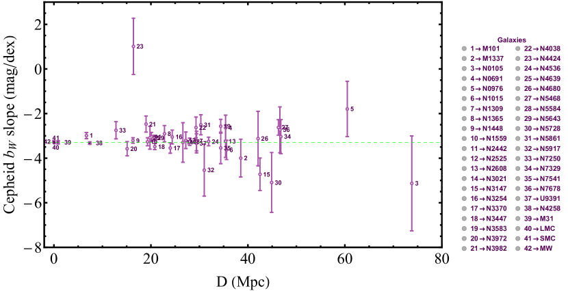
Figure 1: Independently fitted slopes $b_{W,i}$ of the Cepheid P-L relations. Here we have ignored non-diagonal terms of the covariance as was done in R21 in the corresponding Figure 10. There is a consistent trend of most non-anchor hosts to have a best fit absolute slope $|b_{W}|$ that is smaller than corresponding best fit $b_{W}$ of the anchor hosts (above the dotted line). The dotted line corresponds to the best fit value of $b_{W}=b_{W}^{0}+\Delta b_{W}=-0.286-0.013=-0.299$ in the context of the baseline SH0ES analysis as shown in Table 2.

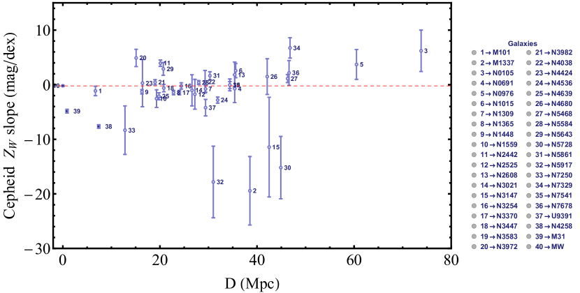
Figure 2: Independently fitted metallicity slopes $Z_{W,i}$ in terms of the distance of the Cepheid host. Clearly the spread of many points is larger than the corresponding uncertainties indicating either inhomogeneities of the sample or underestimation of the uncertainties. In fact, there seems to be a trend of most $|Z_{W,i}|$ absolute slopes to be larger than the corresponding slope of the the Milky Way (MW) (below the dotted line). The dotted line corresponds to the best fit value of $Z_{W}=-0.21$ in the context of the baseline SH0ES analysis as shown in Table 2.

Some inhomogeneities are visible in the distance distribution of both the individual Cepheid slopes in Figs. 1 and 2 as well as in Fig. C.3. For example in Figs. 1 and C.3 there is a consistent trend of most non-anchor hosts to have an absolute best fit slope $b_{W}$ that is smaller than the corresponding best fit $b_{W}$ of the anchor hosts (above the dotted line). Similarly, in Fig. 2 there seems to be a trend of most $Z_{W,i}$ absolute slopes to be larger than the corresponding slope of the the Milky Way (MW) (below the dotted line).

A careful inspection of Figs. 1 and 2 indicates that the scatter is significantly larger than the standard uncertainties of the slopes. Indeed a $\chi^{2}$ fit to a universal slope for $Z_{W}$ of the form

$$\chi^{2}(Z_{W})=\sum_{i=1}^{N}\frac{(Z_{W,i}-Z_{W})^{2}}{\sigma_{Z_{W,i}}^{2}}$$ (28)

leads to a minimum $\chi_{min}^{2}$ per degree of freedom ($dof$) $\frac{\chi^{2}_{ZW,min}}{dof}=22$ (with a best fit $Z_{W,bf}\simeq-1$) while $\frac{\chi^{2}_{min}}{dof}=O(1)$ would be expected for an acceptable fit. Also for $b_{W}$ we find $\frac{\chi^{2}_{bW,min}}{dof}=1.55$ ($b_{W,bf}=-3.3$) which is more reasonable but still larger than 1 indicating a relatively poor quality of fit to a universal slope.

There are two possible causes for this poor quality of fit to universal slopes: either many of uncertainties of the individual host slopes have been underestimated or the universal slope model is not appropriate. In view of the fact that the uncertainties of the Cepheid periods and metallicities have not been included in the $\chi^{2}$ fit because they were not provided by R21 released data we make the working hypothesis that the uncertainties have been underestimated and thus we add a scatter error adjusted so that $\frac{\chi^{2}_{bW,min}}{dof}\simeq\frac{\chi^{2}_{ZW,min}}{dof}\simeq 1$. Thus for $\chi^{2}(Z_{W})$ we have

$$\chi^{2}(Z_{W})=\sum_{i=1}^{N}\frac{(Z_{W,i}-Z_{W})^{2}}{\sigma_{Z_{W,i}}^{2}+\sigma_{Z,scat}^{2}}$$ (29)

For $\frac{\chi^{2}_{ZW,min}}{dof}\simeq 1$ we must set $\sigma_{Z,scat}\simeq 3.2$ which is significantly larger than most uncertainties of individual host $Z_{W}$ slopes. Similarly, for $\frac{\chi^{2}_{bW,min}}{dof}\simeq 1$ we must set $\sigma_{b,scat}\simeq 0.18$ which is comparable or smaller than most uncertainties of individual host $b_{W}$ slopes as shown in Table C.1.

In order to quantify possible inhomogeneities of Cepheid hosts $b_{W,i}$ and $Z_{W,i}$ slopes, we have split each sample of slopes in two bins: a low distance bin with Cepheid host distances $D$ smaller than a critical distance $D_{c}$ and a high distance bin with $D>D_{c}$. Given $D_{c}$, for each bin we find the best fit slope and its standard $1\sigma$ error using the maximum likelihood method. For example for a low distance $b_{W}$ bin we minimize

$$\chi^{2}(b_{W}^{<})=\sum_{i=1}^{N^{<}}\frac{(b_{W,i}-b_{W}^{<})^{2}}{\sigma_{b_{W,i}}^{2}+\sigma_{scat}^{2\,<}}$$ (30)

where $N^{<}$ is the number of hosts in the low distance bin and $\sigma_{scat}$ is the additional uncertainty (scatter error) chosen in each bin so that $\chi^{2}\simeq 1$ so that the fit becomes consistent with a constant $b_{W}$ in each bin. Thus we find the best fit low distance bin slope $b_{W}^{<}$ and its standard error and similarly for the high distance bin $D>D_{c}$, $b_{W}^{>}$ and for the slopes $Z_{W}^{<}$, $Z_{W}^{>}$. Thus for each $D_{c}$ we obtain two best fit slopes (one for each bin) and their standard errors. The level of consistency between the two binned slopes at each $D_{c}$ determines the level of homogeneity and self consistency of the full sample. The results for the best fit binned slopes for $b_{W}$ and $Z_{W}$ are shown in Figs. 3 and 4 respectively as functions of the dividing critical distance $D_{c}$.

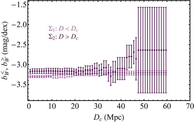
Figure 3: Binned Cepheid P-L slopes $b_{W}^{>}$ and $b_{W}^{<}$ for the high distance bin $\Sigma_{2}$ ($D>D_{c}$) and the low distance bin $\Sigma_{1}$ ($D<D_{c}$) respectively. In each bin $\sigma_{scat}$ was used and adjusted so that $\chi_{bW,min}^{2}\simeq 1$. Notice that for $D_{c}\simeq 50Mpc$, the high-low distance bins are statistically consistent with each other due to small number of Cepheid in the high distance bin, but the difference of their slope best fit values is maximized.

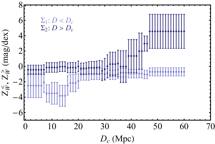
Figure 4: Binned Cepheid metallicity slopes $Z_{W}^{>}$ and $Z_{W}^{<}$ for the high distance bin $\Sigma_{2}$ ($D>D_{c}$) and the low distance bin $\Sigma_{1}$ ($D<D_{c}$) respectively. In each bin the additional scattering uncertainty $\sigma_{scat}$ was used and adjusted so that $\chi_{ZW,min}^{2}\simeq 1$. For $D_{c}\simeq 50Mpc$ the difference between the best fit bin slopes is maximized and the tension between them is larger than $2\sigma$ (see also Fig. 5).

Interestingly, for a range of $D_{c}$ there is a mild tension between the best fit values of the high and low distance bins which reaches levels of $2-3\sigma$ especially for the metallicity slopes $Z_{W}$. For both $b_{W}$ and $Z_{W}$, the absolute value of the difference between the high and low distance bin slopes is maximized for $D_{c}>47Mpc$. For the case of $Z_{W}$ this difference is significant statistically as it exceeds the level of $2\sigma$. The level of statistical consistency between high and low distance bins for both slopes $b_{W}$ and $Z_{W}$ is shown in Fig. 5. In the range of $D_{c}$ between $40Mpc$ and $50Mpc$ and also between $10Mpc$ and $20Mpc$, it is shown that in the case of $Z_{W}$ the $\sigma$-distance

$$\sigma_{d}\equiv\frac{|Z_{W}^{>}-Z_{W}^{<}|}{\sqrt{\sigma_{Z_{W}^{>}}^{2}+\sigma_{Z_{W}^{<}}^{2}}}$$ (31)

between the best fit binned $Z_{W}$ metallicity slopes can reach a level beyond $2\sigma$ (see Figs 4 and 5).

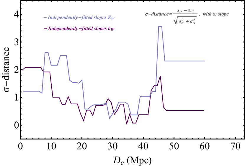
Figure 5: The $\sigma$ distance between the best fit high distance bin ($D>D_{c}$) and low distance bin slopes ($s^{>}(b_{W}^{>},Z_{W}^{>})$ and $s^{<}(b_{W}^{<},Z_{W}^{<})$) defined in Eq. (31) for $Z_{W}$ and similarly for $b_{W}$.

An additional test of possible intrinsic tensions of the Cepheid properties in the SH0ES Cepheid sample is obtained by comparing the probability distributions of the Cepheid period and metallicity for the full sample of the 3130 Cepheid with high and low distance subsamples. In Figs. 6 and 7 we show histograms of the probability distributions of the Cepheid period and metallicity for the whole Cepheid sample and for the high ($D>D_{c}$) and low distance ($D<D_{c}$) subsamples for $D_{c}=50Mpc$. The two subsamples for each observable are clearly inconsistent with each other and with the full sample. This is demonstrated visually and also through the Kolmogorov-Smirnov consistency test which quantifies the inconsistency and gives a p-value very close to 0 for the three sample pairs. However, as communicated to us by members of the SH0ES team (private communication) this inconsistency can be justified by observational selection effects and does not necessarily indicate a physics change at $D_{c}=50Mpc$. For example bright Cepheids have longer periods and they are more easily observed at high distances. Thus it is expected that there will be higher period (brighter) Cepheids observed at higher distances. Other variables such as the timespan of the observations also play a role. For more distant galaxies there is a trend to allow a longer window of observations so that longer period Cepheids can be found. Also the star formation history of the galaxies dictates whether one will have very long period Cepheids which come from massive, short lived stars. However, even though the observed inconsistency in the Cepheid properties probability distributions may be explained using observational biases and anticipated galactic properties, it may also be a hint of interesting new physics and/or systematic effects.

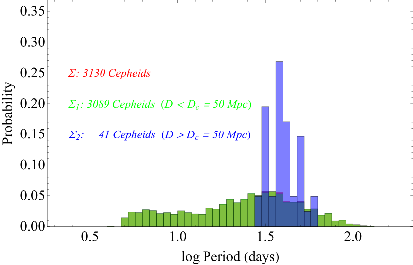
Figure 6: Probability distributions of the Cepheid period for the whole Cepheid sample and for the high ($D>D_{c}$) and low distance ($D<D_{c}$) subsamples for $D_{c}=50Mpc$. Due to the small number of Cepheids in the $D>50Mpc$ bin (41), the probability distribution of the full sample (3130 Cepheids) is almost identical with the the probability distribution of the $D<50Mpc$ bin and thus the light green bars overlap with the red bars.

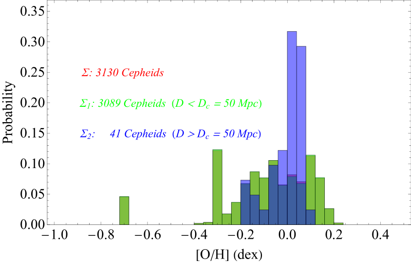
Figure 7: Probability distributions of the Cepheid metallicity for the whole Cepheid sample and for the high ($D>D_{c}$) and low distance ($D<D_{c}$) subsamples for $D_{c}=50Mpc$. Due to the small number of Cepheids in the $D>50Mpc$ bin (41), the probability distribution of the full sample (3130 Cepheids) is almost identical with the the probability distribution of the $D<50Mpc$ bin and thus the light green bars overlap with the red bars.

In view of the above identified level of mild inhomogeneities identified is the SH0ES data, it would be interesting to extend the SH0ES modeling of the Cepheids and SnIa with new degrees of freedom that can model the data taking into account these inhomogeneities. This is the goal of the next section.

3 Generalized analysis: New degrees of freedom allowing for a physics transition.

An obvious generalization of the SH0ES analysis described in subsection 2.1 which models the Cepheid-SnIa luminosities using four main parameters is to allow for a transition of any one of these parameters at a particular distance or equivalently cosmic time when radiation was emitted. Such a transition could be either a result of a sudden change in a physics constant (e.g. the gravitational constant) during the last $200Myrs$ in the context e.g. of a first order phase transition or a result of the presence of an unknown systematic.

Another modification of the standard SH0ES analysis in R21 would be to extend the number of constraints imposed on the data vector $\bf{Y}$ taking into account other cosmological data like the inverse distance ladder estimate of $M_{B}$ Camarena and Marra (2021); Marra and Perivolaropoulos (2021); Gómez-Valent (2022). Both of these generalizations will be implemented in the present section.

3.1 Allowing for a transition of a Cepheid calibration parameter

A transition of one of the Cepheid calibration parameters can be implemented by replacing one of the four modeling parameters in the $\bf{q}$ vector by two corresponding parameters: one for high and one for low distances (recent cosmic times). Thus, in this approach the number of parameters and entries in the parameter vector $\bf{q}$ increases by one from 47 to 48. Since one of the entries of $\bf{q}$ is replaced by two entries, the corresponding column of the modeling matrix $\bf{L}$ should be replaced by two columns. The high distance parameter column should be similar to the original column it replaced but with zeros in entries corresponding to low distance data (or constraints) and the reverse should happen for the low distance parameter column. This process is demonstrated in the following schematic diagram where the $q_{j}$ parameter is replaced by the two parameters $q_{j}$ (or $q_{j}^{<}$) and $q_{j+1}$ (or $q_{j}^{>}$) and the $j$ column of $\bf{L}$ is replaced by the $j$ and $j+1$ corresponding columns which have zeros in the low or high distance data (or constraint) entries.

$$\bf{L_{(3492\times 47)}}=\left(\begin{array}[c]{ccc}\ldots&L_{1,j}&\ldots\\ \ldots&L_{2,j}&\ldots\\ \ldots&L_{3,j}&\ldots\\ \ldots&\ldots&\ldots\\ \ldots&\ldots&\ldots\\ \ldots&L_{3491,j}&\ldots\\ \ldots&L_{3492,j}&\ldots\\ \end{array}\right)$$

(32)

$${\bf q_{(47\times 1)}}=\begin{pmatrix}\ldots\\ \ldots\\ q_{j}\\ \ldots\\ \ldots\\ \end{pmatrix}\rightarrow\bf q_{(48\times 1)}=$$

(33)

In this manner, if the parameter $b_{W}$ was to be split to $b_{W}^{>}$ and $b_{W}^{<}$ for example, Eq. (6) would be replaced by

$$m_{H,i,j}^{W}(D)=\mu_{i}+M_{H}^{W}+b_{W}^{>}\Theta(D-D_{c})[P]_{i,j}+b_{W}^{<}\Theta(D_{c}-D)[P]_{i,j}+Z_{W}[O/H]_{i,j}$$ (34)

and similarly for splittings of each one the other three parameters $M_{H}^{W}$, $Z_{W}$ and $M_{B}$. In (34) $D$ is a distance that may be assigned to every entry of the data-vector $\bf{Y}$ (Cepheids, SnIa and constraints). Notice that the splitting of any parameter to a high and low distance version does not affect the form of the $\bf{Y}$ data vector and the covariance matrix $\bf{C}$ of the data. In order to properly place the 0 entries of each one of the new columns, a distance must be assigned to every entry of $\bf{Y}$. We have specified this distance for each host using the literature resources or the best fit distance moduli of each host. These distances along with other useful properties of the Cepheids used in our analysis are shown in Table 3.

Table 3: Properties of the Cepheid hosts considered in the analysis.

Galaxy	SnIa	Ranking in	Ranking in	Ranking in	$D$ a	Number of fitted	Initial point	Final point
		Fig. C.3	Table 3 in R21	Data Vector Y	$[Mpc]$	Cepheids	in Vector Y	in Vector Y
M101	2011fe	8	1	1	6,71	259	1	259
M1337	2006D	34	2	2	38,53	15	260	274
N0691	2005W	28	4	3	35,4	28	275	302
N1015	2009ig	24	6	4	35,6	18	303	320
N0105	2007A	42	3	5	73,8	8	321	328
N1309	2002fk	25	7	6	29,4	53	329	381
N1365	2012fr	20	8	7	22,8	46	382	427
N1448	2001el,2021pit	7	9	8	16,3	73	428	500
N1559	2005df	11	10	9	19,3	110	501	610
N2442	2015F	13	11	10	20,1	177	611	787
N2525	2018gv	21	12	11	27,2	73	788	860
N2608	2001bg	31	13	12	35,4	22	861	882
N3021	1995al	35	14	13	26,6	16	883	898
N3147	1997bq,2008fv,2021hpr	32	15	14	42,5	27	899	925
N3254	2019np	16	16	15	24,4	48	926	973
N3370	1994ae	14	17	16	24	73	974	1046
N3447	2012ht	9	18	17	20,8	101	1047	1147
N3583	2015so	15	19	18	34,4	54	1148	1201
N3972	2011by	17	20	19	15,1	52	1202	1253
N3982	1998aq	19	21	20	19	27	1254	1280
N4038	2007sr	29	22	21	29,3	29	1281	1309
N4424	2012cg	40	23	22	16,4	9	1310	1318
N4536	1981B	12	24	23	31,9	40	1319	1358
N4639	1990N	27	25	24	19,8	30	1359	1388
N4680	1997bp	38	26	25	42,1	11	1389	1399
N5468	1999cp,2002cr	18	27	26	46,3	93	1400	1492
N5584	2007af	10	28	27	28	165	1493	1657
N5643	2013aa,2017cbv	6	29	28	20,7	251	1658	1908
N5728	2009Y	41	30	29	44,9	20	1909	1928
N5861	2017erp	26	31	30	30,3	41	1929	1969
N5917	2005cf	37	32	31	31	14	1970	1983
N7250	2013dy	22	33	32	12,8	21	1984	2004
N7329	2006bh	33	34	33	46,8	31	2005	2035
N7541	1998dh	30	35	34	34,4	33	2036	2068
N7678	2002dp	36	36	35	46,6	16	2069	2084
N0976	1999dq	39	5	36	60,5	33	2085	2117
U9391	2003du	23	37	37	29,4	33	2118	2150
Total						2150	1	2150
N4258	Anchor	4	38	38	7,4	443	2151	2593
M31	Supporting	5	39	39	0,86	55	2594	2648
LMCb	Anchor	2	40	40	0,05	270	2649	2918
SMCb	Supporting	3	41	41	0,06	143	2919	3061
LMCc	Anchor	2	40	42	0,05	69	3062	3130
Total						980	2151	3130
Total All						3130	1	3130

NOTE - (a) Distances from NASA/IPAC Extragalactic Database. (b) From the ground. (c) From HST.

We have thus considered four generalizations of the baseline SH0ES analysis each one corresponding to a high-low distance split of each one of the four modeling parameters. For each generalization we obtained the best fit values and uncertainties of all 48 parameters of the generalized parameter vector $\bf{q}$ for several values of the critical distance $D_{c}\in[1,60Mpc]$ which defined in each case the high-low distance data bins. The best fit values with uncertainties for the high-low $D$ split parameter (green and blue points) and for $H_{0}$ (red points), for each generalization considered, is shown in Figs 8, 9, 10 and 11 in terms of $D_{c}$. Dotted lines correspond to the SH0ES R21 $H_{0}$ best fit and to the Planck18/$\Lambda$CDM best fit for $H_{0}$. The following comments can be made on the results of Figs 8, 9, 10 and 11.

• When the SnIa absolute magnitude $M_{B}$ is allowed to change at $D_{c}$ ($M_{B}$ transition) and for $D_{c}>47Mpc$, the best fit value of $H_{0}$ drops spontaneously to the best fit Planck18/$\Lambda$CDM value albeit with larger uncertainty $67.33\pm 4.65$ (see Fig. 8 and second row of Table 4). This remarkable result appears with no prior or other information from the inverse distance ladder results. Clearly, there are increased uncertainties of the best fit parameter values for this range of $D_{c}$ because the most distant usable Cepheid hosts are at distances $46.8Mpc$ (N7329), $60.5Mpc$ (N0976) and $73.8Mpc$ (N0105) and only two of them are at distance beyond $47Mpc$. These hosts (N0975 and N0105) have a total of 41 Cepheids and 4 SnIa. Due to the large uncertainties involved there is a neutral model preference for this transition degree of freedom at $D_{c}>47Mpc$ (the small drop of $\chi^{2}$ by $\Delta\chi^{2}\simeq-1.5$ is balanced by the additional parameter of the model). This however changes dramatically if the inverse distance ladder constraint on $M_{B}$ is included in the vector $\bf{Y}$ as discussed below.

• For all four modeling parameters considered, there is a sharp increase in the absolute difference between the high-low distance best fit parameter values for $D_{c}\gtrsim 47Mpc$. The statistical significance of this split however is low due to the relatively small number of available Cepheids at $D>47Mpc$.

• The best fit value of $H_{0}$ changes significantly when the SnIa absolute magnitude $M_{B}$ is allowed to make a transition at $D_{c}>47Mpc$ but is not significantly affected if the three Cepheid modeling parameters $M_{W}$, $b_{W}$ and $Z_{W}$ are allowed to make a transition at any distance. This is probably due to the large uncertainties involved and due to the fact that $H_{0}$ is only indirectly connected with the three Cepheid modeling parameters.

• Each one of the transition degrees of freedom mildly reduces $\chi^{2}$ thus improving the fit to the data but these transition models are not strongly preferred by model selection criteria which penalize the extra parameter implied by these models. This is demonstrated in Figs. 12, 13 which show the values of $\Delta\chi^{2}_{min}$, $\Delta AIC$ and $\Delta BIC$ of the four transition models with respect to the baseline SH0ES model for various $D_{c}$ transition distances. As discussed below this changes dramatically if the inverse distance ladder constraint on $M_{B}$ is introduced in the analysis.

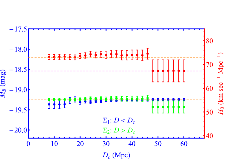
Figure 8: The best fit values with uncertainties for the high-low $D$ bin of SnIa absolute magnitude $M_{B}$ (green and blue points) and for $H_{0}$ (red points). This generalization of the SH0ES baseline analysis allows for a transition of $M_{B}$. The best fit parameter values as shown as functions of the critical transition $D_{c}$. Dotted lines correspond to the SH0ES R21 best fit and to the Planck18/$\Lambda$CDM best fit for $H_{0}$.

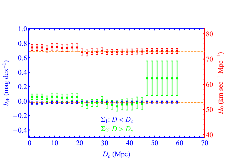
Figure 9: Same as Fig. 8 in an analysis generalization where the parameter $b_{W}$ is allowed to have a transition at a distance $D_{c}$. Notice the sharp increase in the difference between best fit parameters high of $D$ and low $D$ bin $|b_{W}^{>}-b_{W}^{<}|$ for $D_{c}>47Mpc$.

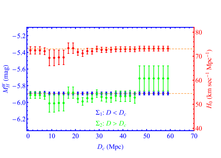
Figure 10: Same as Fig. 8 in an analysis generalization where the parameter $M_{W}$ is allowed to have a transition at a distance $D_{c}$. Notice the sharp increase in the difference between best fit parameters of high $D$ and low $D$ bin $|M_{W}^{>}-M_{W}^{<}|$ for $D_{c}>47Mpc$.

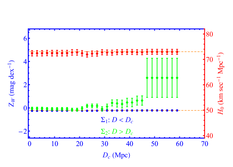
Figure 11: Same as Fig. 8 in an analysis generalization where the parameter $Z_{W}$ is allowed to have a transition at a distance $D_{c}$. Notice the sharp increase in the difference between best fit parameters of high $D$ and low $D$ bin $|Z_{W}^{>}-Z_{W}^{<}|$ for $D_{c}>47Mpc$. The best fit value of the Hubble parameter (red points) is not significantly affected by this type of degree of freedom perhaps due to the indirect connection of $Z_{W}$ with $H_{0}$.

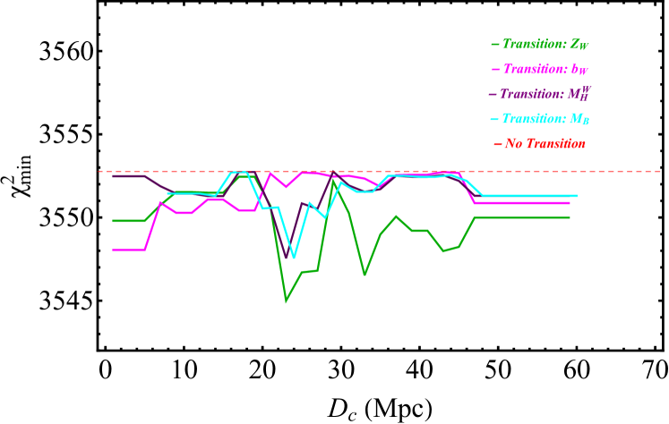
Figure 12: The values of $\Delta\chi^{2}_{min}$ in terms of $D_{c}$ for the four transition models considered with respect to the SH0ES baseline model. No inverse distance ladder constraint on $M_{B}$ has been used for either the baseline or the transition models. The small improvement of the fit to the data is not enough to justify any model preference.

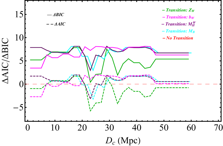
Figure 13: The values of $\Delta AIC$ and $\Delta BIC$ in terms of $D_{c}$ for the four transition models considered with respect to the SH0ES baseline model. No inverse distance ladder constraint on $M_{B}$ has been used for either the baseline or the transition models. The small improvement of the $\chi^{2}$ fit to the data is not enough to justify any model preference. In fact the BIC which strongly penalizes any additional parameter mildly disfavors the transition models.

3.2 The effect of the inverse distance ladder constraint

In view of the spontaneous transition of the SnIa absolute magnitude $M_{B}$ that appears to lead to a Hubble tension resolution, while being mildly favored by the SH0ES data ($\Delta\chi^{2}\simeq-1.5$) without any inverse distance ladder information included in the fit, the following question arises:

How does the level of preference for the $M_{B}$ transition model (compared to the SH0ES baseline model) change if an additional constraint is included in the analysis obtained from the inverse distance ladder best fit for $M_{B}$?

The inverse distance ladder constraint on $M_{B}$ is Camarena and Marra (2021); Marra and Perivolaropoulos (2021); Gómez-Valent (2022)

$$M_{B}^{P18}=-19.401\pm 0.027$$ (35)

In order to address this question we modify the analysis by adding one more constraint to the $\bf{Y}$ data-vector: after entry 3215 which corresponds to the 8th constraint we add the value -19.401 for the $M_{B}$ constraint. We also add a line to the model matrix $\bf{L}$ after line 3215 with all entries set to zero except the entry at column 43 corresponding to the parameter $M_{B}^{<}$. A column after column 43 is added in $\bf{L}$ to accommodate the high distance parameter $M_{B}^{>}$ as described above. The new constraint is assigned a large distance (larger than the distance of the most distant SnIa of the sample) so that it only affects the high distance parameter $M_{B}^{>}$ (the entry at line 3216 column 43 of $\bf{L}$ is set to 0 for all $D_{c}$ while the entry at column 44 of the same line is set to 1 for all $D_{c}$). To accommodate the corresponding uncertainty of the new constraint we also add a line at the covariance matrix after line 3215 with a single nonzero entry at the diagonal equal to $\sigma_{MB}^{2}=0.027^{2}=0.000729$. Thus after the implementation of the constraint in the $M_{B}$ transition model the $\bf{Y}$ vector has 3493 entries, the $\bf{L}$ model matrix has dimensions $3493\times 48$, the $\bf{q}$ parameter vector has $48$ entries and the covariance matrix $\bf{C}$ matrix has dimensions $3493\times 3493$. In a similar way we may implement the constraint (35) in the SH0ES model without allowing for the additional transition degree of freedom and implement model selection criteria to compare the baseline with the transition model in the presence of the inverse distance ladder constraint.

The new constraints on $H_{0}$ and on the parameters $M_{B}^{<}$, $M_{B}^{>}$ emerging from this modified modeling analysis are shown in Fig. 14 in terms of $D_{c}$. The corresponding quality of fit expressed via the value of $\chi_{min}^{2}$ and model selection Kerscher and Weller (2019); Liddle (2007) expressed via the AIC Akaike (1974) and BIC criteria is shown in Fig. 15. The definitions and properties of the AIC and BIC criteria are described in Appendix D

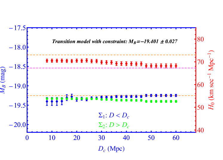
Figure 14: The new constraints on $H_{0}$ and on the parameters $M_{B}^{<}$, $M_{B}^{>}$ emerging after implementing the inverse distance ladder constraint (35) on the high distance bin of the $M_{B}$ transition model.

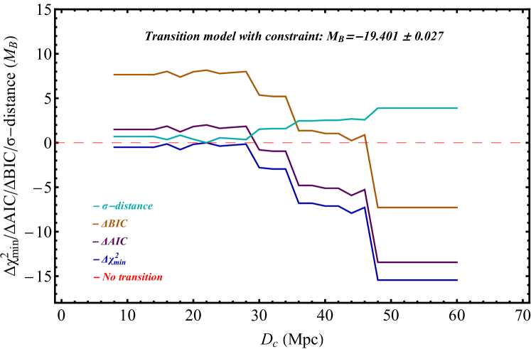
Figure 15: Model selection criteria of the $M_{B}$ transition model with respect to the baseline SH0ES model in the presence of the inverse distance ladder constraint (35). The $\sigma$-distance between the low distance best fit $M_{B}^{<}$ and the high distance $M_{B}^{>}$ is also plotted in terms of $D_{c}$. Clearly the $M_{B}$ transition model is strongly preferred with respect to the SH0ES baseline (no transition) model especially for transition distances $D_{c}\simeq 50Mpc$.

Clearly, the transition degree of freedom at $D_{c}\simeq 50Mpc$ which is mildly preferred by the data even in the absence of the inverse distance ladder constraint, is strongly preferred by the data in the presence of the constraint while the $\sigma$-distance between the low distance best fit parameter $M_{B}^{<}$ and the high distance $M_{B}^{>}$ reaches a level close to $4\sigma$. These results are described in more detail in Table 4. The full list of the best fit values of all the parameters of the vector $\bf{q}$ for the SH0ES baseline model with and without the inverse distance ladder constraint in the data vector $\bf{Y}$ is shown in Table 2 along with the corresponding uncertainties.

Table 4: A model comparison (baseline vs transitions) and best fit parameter values in the absence (top five rows) and in the presence (last two rows) of the inverse distance ladder constraint. Notice that in the presence of the inverse distance ladder constraint and the transition degree of freedom, the best fit value of $H_{0}$ is identical with the inverse distance ladder result of the completed SDSS-IV extended BAO survey Alam et al. (2021).

Model	$\chi^{2}_{min}$	$\chi_{red}^{2}$ a	$\Delta AIC$	$\Delta BIC$	$H_{0}$	$M_{B}$	$M_{H}^{W}$	$\Delta b_{W}$	$Z_{W}$
					$[Km\,s^{-1}\,Mpc^{-1}]$	$[mag]$	$[mag]$	$[mag/dex]$	$[mag/dex]$
Baseline	3552.76	1.031	0	0	$73.043\pm 1.007$	$-19.253\pm 0.029$	$-5.894\pm 0.018$	$-0.013\pm 0.015$	$-0.217\pm 0.045$
Transitionb $M_{B}$	3551.31	1.031	0.55	6.71	$67.326\pm 4.647$	$-19.250\pm 0.029$	$-5.894\pm 0.018$	$-0.013\pm 0.015$	$-0.217\pm 0.045$
						$-19.430\pm 0.150$
						$1.2\sigma$
Transitionb $M_{H}^{W}$	3551.31	1.031	0.55	6.71	$73.162\pm 1.014$	$-19.250\pm 0.029$	$-5.894\pm 0.018$	$-0.013\pm 0.015$	$-0.217\pm 0.045$
							$-5.713\pm 0.151$
							$1.2\sigma$
Transitionb $Z_{W}$	3549.99	1.030	-0.77	5.39	$72.981\pm 1.007$	$-19.255\pm 0.029$	$-5.894\pm 0.018$	$-0.014\pm 0.015$	$-0.217\pm 0.045$
									$\;\;2.588\pm 1.686$
									$1.7\sigma$
Transitionb $b_{W}$	3550.86	1.030	0.10	6.26	$73.173\pm 1.013$	$-19.249\pm 0.029$	$-5.894\pm 0.018$	$-0.013\pm 0.015$	$-0.217\pm 0.045$
								$\;\;\>0.315\pm 0.239$
								$1.4\sigma$
Baseline+Constraintc	3566.78	1.035	0	0	$70.457\pm 0.696$	$-19.332\pm 0.020$	$-5.920\pm 0.017$	$-0.026\pm 0.015$	$-0.220\pm 0.045$
Transitionb,c $M_{B}$+Constraint	3551.34	1.031	-13.44	-7.27	$68.202\pm 0.879$	$-19.249\pm 0.029$	$-5.893\pm 0.018$	$-0.013\pm 0.015$	$-0.217\pm 0.045$
						$-19.402\pm 0.027$
						$3.9\sigma$

NOTE - (a) $\chi_{red}^{2}=\chi_{min}^{2}/dof$, where $dof=N-M$ is typically the number of degrees of freedom (with $N$ the number of datapoints used in the fit and $M$ the number of free parameters) for each model. (b) At critical distance $D_{c}\simeq 50Mpc$. (c) With constraint $M_{B}=-19.401\pm 0.027$.

The following comments can be made on the results shown in Table 4.

• The $M_{B}$ transition degree of freedom resolves the $H_{0}$ tension both in the absence of the inverse distance ladder constraint (second raw of Table 4) and in the presence of it (last row of Table 4).

• In the presence of the inverse distance ladder constraint, the model with the $M_{B}$ transition degree of freedom at $D_{c}=50Mpc$ is strongly preferred over the baseline $SH0ES$ model as indicated by the model selection criteria despite the additional parameter it involves (comparison of the last two rows of Table 4).

• The transition degree of freedom when allowed in each one of the other three modeling parameters does not lead to a spontaneous resolution of the Hubble tension since the best fit value of $H_{0}$ is not significantly affected. However, it does induce an increased absolute difference between the best fit values of the high distance and low distance parameters which however is not statistically significant due to the large uncertainties of the bin with $D>D_{c}\simeq 50Mpc$ (see also Figs. 9, 10 and 11).

The above comments indicate that interesting physical and or systematic effects may be taking place at distances at or beyond $50Mpc$ in the SH0ES data and therefore more and better quality Cepheid/SnIa data are needed at these distances to clarify the issue. This point is further enhanced by the recent study of Ref. Wojtak and Hjorth (2022) indicating that SnIa in the Hubble flow (at distances $D>90Mpc$) appear to have different color calibration properties than SnIa in Cepheid hosts (at distances $D<75Mpc$).

The hints for a transition in the SnIa absolute luminosity and magnitude $M_{B}$ are also demonstrated in Fig. 16 where we show the mean SnIa absolute magnitude $M_{Bi}$ for each Cepheid+SnIa host $i$ obtained from the equation

$$M_{Bi}=m_{Bi}^{0}-\mu_{i}$$ (36)

where $m_{Bi}^{0}$ is the measured apparent magnitude of the SnIa and $\mu_{i}$ are the best fit distance host distance moduli obtained using the SH0ES baseline model (left panel of Fig. 16) and the $M_{B}$ transition model (right panel) which allows (but does not enforce) an $M_{B}$ transition at $D_{c}=50Mpc$. Notice that when the $M_{B}$ transition degree of freedom is allowed in the analysis the best fit values of $M_{Bi}$ for the more distant hosts N0976 ($D=60.5Mpc$) and N0105 ($D=73.8Mpc$) spontaneously drop to the inverse distance ladder calibrated value range.

The inverse distance ladder calibrated values of the absolute magnitudes $M_{Bi}$ of SnIa in the Hubble flow are obtained by assuming $H_{0}=H_{0}^{P18}=67.36\pm 0.54$ km s^-1 Mpc^-1 and using the following equation

$$M_{Bi}=m(z_{Bi}^{0})+5\log_{10}\left[H_{0}^{P18}\cdot Mpc/c\right]-5\log_{10}\left[D_{L}(z_{i})\right]-25$$ (37)

where $D_{L}(z_{i})$ is the Hubble free luminosity distance in the context of Planck18/$\Lambda$CDM and $m(z_{Bi}^{0})$ are the binned corrected SnIa apparent magnitudes of the Pantheon sample. The corresponding binned Cepheid+SnIa host values of $M_{B}$ obtained assuming the baseline Sh0ES model (red points) and the $M_{B}$ transition model ($D_{c}=50Mpc$, green points) are shown in Fig. 17 along with the inverse distance ladder calibrated binned $M_{B}$ of the Hubble flow SnIa of the Pantheon dataset (blue points). When the transition dof is allowed, the data excite it and a hint for a transition appears (the green data point is of the transition model is clearly below the red point corresponding to the constant $M_{B}$ SH0ES baseline model) even though the statistical significance of the indicated transition is low due to the small number of Cepheids (41) included in the last bin with $D\in[50Mpc,75Mpc]$.

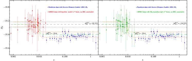
Figure 16: The mean SnIa absolute magnitude $M_{Bi}$ for each Cepheid+SnIa host $i$ obtained from Eq. (36), obtained using the SH0ES baseline model (left panel) and the $M_{B}$ transition model (right panel) which allows (but does not enforce) an $M_{B}$ transition at $D_{c}=50Mpc$. Notice that when the $M_{B}$ transition degree of freedom is allowed in the analysis the best fit values of $M_{Bi}$ for the more distant hosts N0976 ($D=60.5Mpc$) and N0105 ($D=73.8Mpc$) spontaneously drop to the inverse distance ladder calibrated value range (green points with $z>0.01$).

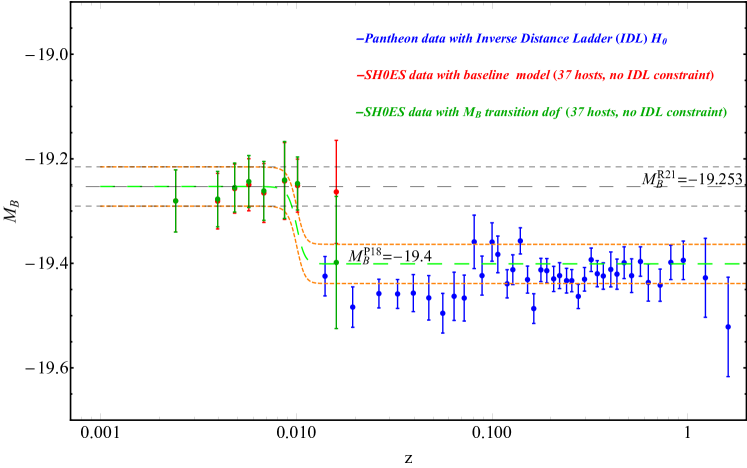
Figure 17: The binned (5 host bins with 2 hosts in last bin where $z>0.01$) Cepheid+SnIa host values of $M_{B}$ obtained assuming the baseline SH0ES model (red points) and the $M_{B}$ transition model ($D_{c}=50Mpc$, green points) are shown along with the inverse distance ladder calibrated binned $M_{B}$ of the Hubble flow SnIa of the Pantheon dataset (blue points). When the transition dof is allowed, the data excite it and a hint for a transition appears (the green data point of the transition model is clearly below the red point corresponding to the constant $M_{B}$ SH0ES baseline model).

4 Conclusion

We have described a general framework for the generalization of the Cepheid+SnIa modeling in the new SH0ES data. Such modeling generalization approach is motivated by the increased statistical significance of the Hubble tension and may hint towards new degrees of freedom favored by the data. Such degrees of freedom may be attributed to either new physics or to unknown systematics hidden in the data.

In the present analysis we have focused on a particular type of new modeling degree of freedom allowing for a transition of any one of the four Cepheid/SnIa modeling parameters at a distance $D_{c}$. However, our analysis can be easily extended to different degrees of freedom with physical motivation. Examples include possible modeling parameter dependence on properties other than distance (e.g. dust extinction, color and stretch calibration properties etc.). In addition other degrees of freedom that could be excited by the data could involve the modeling parameters that have been absorbed in the R21 SH0ES data like the Cepheid dust extinction parameter $R_{W}$ and the color and stretch SnIa calibration parameters $\beta$ and $\alpha$. These degrees of freedom may also be probed and excited by the fit to the data if allowed by the modeling Wojtak and Hjorth (2022).

We have demonstrated that our proposed transition degrees of freedom are mildly excited by the SH0ES data and in the case of the SnIa absolute magnitude $M_{B}$ transition degree of freedom at $D_{c}\simeq 50Mpc$, the best fit value of $H_{0}$ shifts spontaneously to a value almost identical with the Planck18/$\Lambda$CDM best fit value thus annihilating the Hubble tension. However, the high distance bin in this case involves only 41 Cepheids and 4 SnIa and therefore the best fit value of $M_{B}^{>}$ which effectively also fixes $H_{0}$ involves significant uncertainties.

In the presence of the inverse distance ladder constraint on the high distance bin parameter $M_{B}^{>}$ of the $M_{B}$ transition model and on the single $M_{B}$ parameter of the SH0ES model, the uncertainties reduce dramatically. The Hubble tension is fully resolved only in the presence of the $M_{B}$ transition degree of freedom at $D_{c}\simeq 50Mpc$. This transition model is also strongly selected over the baseline SH0ES model with the constraint, by both model selection criteria AIC and BIC despite the penalty imposed by AIC and especially BIC on the additional parameter involved in the new modeling. This behavior along with other recent studies Wojtak and Hjorth (2022) hints towards the need of more detailed Cepheid+SnIa calibrating data at distances $D\gtrsim 50Mpc$ i.e. at the high end of rung 2 on the distance ladder.

Our comprehensively described generalized modeling approach opens a new direction in the understanding of the Hubble tension and may be extended by the introduction of a wide range of new degrees of freedom in the SH0ES data analysis and also by the introduction of new constraints motivated by other cosmological data. Such extensions could for example involve more distance bins in the distance dependence of the four main modeling parameters. In that case the relevant column of the modeling matrix $\bf{L}$ would have to be replaced by more than two columns (one for each distance bin). Such bins could also be defined not in terms of distance but in terms of other Cepheid/SnIa properties (e.g. Cepheid metallicity or period and/or SnIa light curve color or stretch). In addition, other parameters beyond the four basic modeling parameters may be considered including the dust extinction parameter $R_{W}$ and/or the SnIa light curve color and stretch parameters. Also, similar modeling generalizations may be implemented on different distance calibrator data used for the measurement of $H_{0}$ such as the TRGB data Freedman et al. (2019).

Physical motivation is an important factor for the evaluation of any new modeling degree of freedom especially if it is favored by the data. A transition of the SnIa luminosity at a particular recent cosmic time could be induced by a sudden change of the value of a fundamental physics constant e.g. the gravitational constant in the context of a recent first order phase transition Coleman (1977); Callan and Coleman (1977); Patwardhan and Fuller (2014) to a new vacuum of a scalar-tensor theory or in the context of a generalization of the symmetron screening mechanism Perivolaropoulos and Skara (2022). A similar first order transition is implemented in early dark energy models Niedermann and Sloth (2020) attempting to change the last scattering sound horizon scale without affecting other well constrained cosmological observables. Thus, even though no relevant detailed analysis has been performed so far, there are physical mechanisms that could potentially induce the SnIa luminosity transition degree of freedom.

The emerging new puzzles challenging our standard models may soon pave the way to exciting discoveries of new physical laws. The path to these discoveries goes through the deep and objective understanding of the true information that is hidden in the cosmological data. The present analysis may be a step in that direction.

—————————————————–

This work was supported by the Hellenic Foundation for Research and Innovation (HFRI - Progect No: 789).

The numerical analysis files for the reproduction of the figures can be found in the A reanalysis of the SH0ES data for $H_{0}$ GitHub repository under the MIT license.

Appendix A Covariance Matrix

A schematic form of the non-diagonal covariance matrix used in our analysis is shown below. The symbols $\sigma_{tot,i}^{2}$ indicate the (non-diagonal in general) covariance submatrix within the $i$ host while the symbols $Z_{cov}$ indicate submatrices that correlate the uncertainties between different hosts.

Appendix B : Analytic minimization of $\chi^{2}$.

The proof of Eqs. (19) and (20) that lead to the best fit parameter values and their uncertainties through the analytic minimization of $\chi^{2}$ may be sketched as follows:
Using the matrix of measurements (data vector) $\bf{Y}$, the matrix of parameters $\bf{q}$ and the equation (or design) matrix $\bf{L}$ with the measurement error matrix (covariance matrix) $\bf{C}$ the $\chi^{2}$ statistic is expressed as

$$\chi^{2}=(\bf{Y}-\bf{Lq})^{T}\bf{C}^{-1}(\bf{Y}-\bf{Lq})=\bf{q}^{T}\bf{L}^{T}\bf{C}^{-1}\bf{L}\bf{q}-2\bf{q}^{T}\bf{L}^{T}\bf{C}^{-1}\bf{Y}+\bf{Y}^{T}\bf{C}^{-1}\bf{Y}$$ (38)

The $\chi^{2}$ is minimized with respect to the parameters $\bf{q}$, by solving the equation

$$\frac{\partial\chi^{2}}{\partial\bf{q}}\Big{|}_{{\bf q}_{best}}=0=>2\bf{L}^{T}\bf{C}^{-1}\bf{L}{\bf q}_{best}-2\bf{L}^{T}\bf{C}^{-1}\bf{Y}=0$$ (39)

Thus the maximum-likelihood parameters are given as

$${\bf q}_{best}=(\bf{L}^{T}\bf{C}^{-1}\bf{L})^{-1}\bf{L}^{T}\bf{C}^{-1}\bf{Y}$$ (40)

We have tested the validity of this equation numerically by calculating $\chi^{2}$ for the SH0ES baseline model and showing that indeed it has a minimum at the analytically predicted parameter values provided by (40). This is demonstrated in Fig. B.1 where we show $\chi^{2}(H_{0})$ with the rest of the parameters fixed at their analytically predicted best fit values. As expected the minimum is obtained at the analytically predicted value of $H_{0}$.

The standard errors squared of the parameters in $\bf{q_{best}}$ are given as the diagonal elements of the transformed covariance matrix

$$\bf{\varSigma_{kl}}=\sum_{i}\sum_{j}\left[\frac{\partial{\bf q}_{best,k}}{\partial Y_{i}}\right]\bf{C_{ij}}\left[\frac{\partial{\bf q}_{best,l}}{\partial Y_{j}}\right]$$ (41)

or

$$\bf{\varSigma}=\left[\frac{\partial{\bf q}_{best}}{\partial Y}\right]\bf{C}\left[\frac{\partial{\bf q}_{best}}{\partial Y}\right]^{T}$$ (42)

Thus

$${}\bf{\varSigma} =(\bf{L}^{T}\bf{C}^{-1}\bf{L})^{-1}\bf{L}^{T}\bf{C}^{-1}C\left[(\bf{L}^{T}\bf{C}^{-1}\bf{L})^{-1}\bf{L}^{T}\bf{C}^{-1}\right]^{T}$$ (43)

$$=(\bf{L}^{T}\bf{C}^{-1}\bf{L})^{-1}\bf{L}^{T}\bf{C}^{-1}C\bf{C}^{-1}\bf{L}(\bf{L}^{T}\bf{C}^{-1}\bf{L})^{-1}$$ (44)

$$=(\bf{L}^{T}\bf{C}^{-1}\bf{L})^{-1}$$ (45)

The standard errors provided by the this equation for the SH0ES baseline model are consistent and almost identical with the published results of R21.

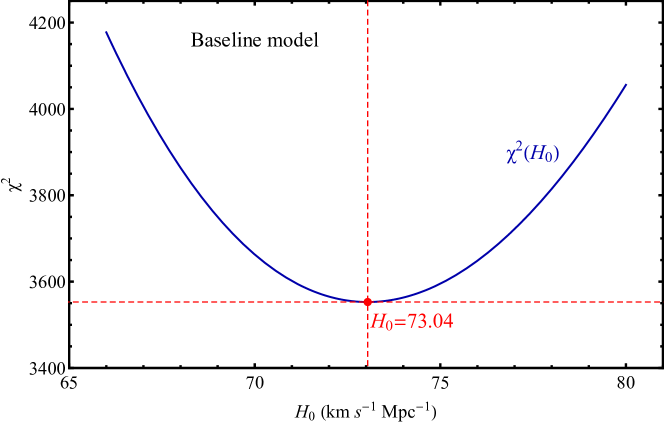
Figure B.1: The form of $\chi^{2}(H_{0}$) for the SH0ES baseline model has a minimum at the analytically predicted value of $H_{0}$ provided by (40) ( the rest of the parameters were fixed at their analytically predicted best fit values).

Appendix C : Reanalysis of Individual Cepheid $m_{H}^{W}$ slope data.

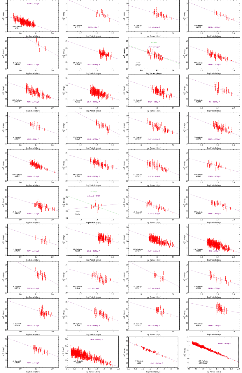
Figure C.1: Fitting individual slopes $b_{W}$ of the $m_{H}^{W}-\log P$, P-L relations for 40 Cepheid hosts: 37 SnIa+Cepheid hosts, 2 anchors (N4258+LMC/SMC) and the pure Cepheid host M31. In the case of the SnIa+Cepheid host N4424 our fit (purple line) is not in agreement with the fit of R21 (green line). In all other cases the agreement is very good.

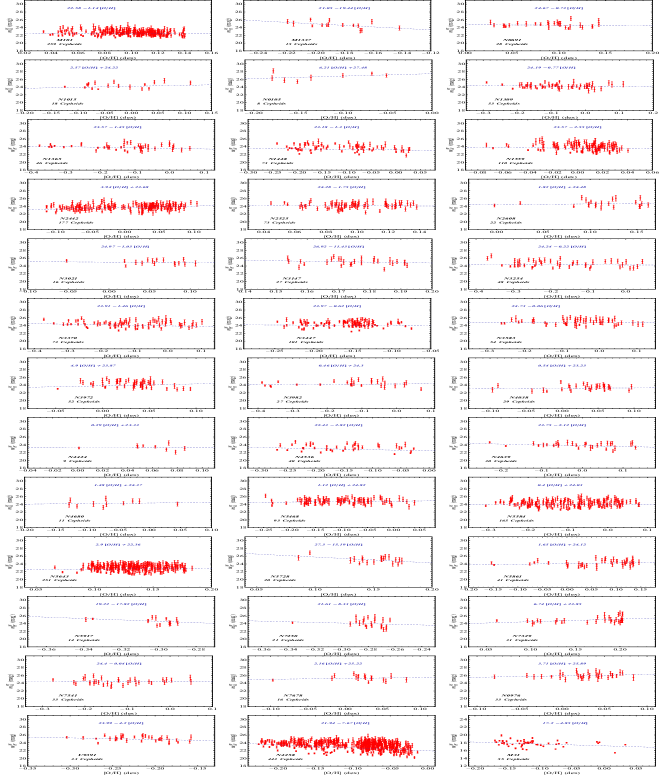
Figure C.2: Fitting individual slopes $Z_{W}$ of the $m_{H}^{W}$ metallicity relations to Cepheid data for the hosts where individual Cepheid metallicity data were provided by R21 (only an average metallicity was provided for LMC/SMC and thus these Cepheid hosts are not included in the plot). Thus the 39 hosts shown correspond to the 37 SnIa+Cepheid hosts, the anchor N4258 and the pure Cepheid host M31.

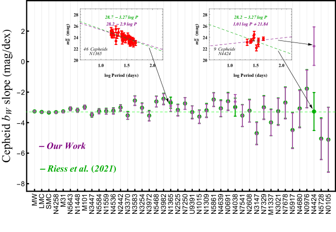
Figure C.3: Independently-fitted slopes $b_{W}$ of the $m_{H}^{W}$ P-L relations (without background covariance of any pair of Cepheids as was done in R21 i.e. taking into account only diagonal terms of the covariance matrix). The points in green are the corresponding points shown in Fig. 10 of R21 (obtained using plot digitizer). Our fits are in excellent agreement with R21 with the exception of 3 points corresponding to hosts N4424, N4038 and N1365. For N4424 there is no point shown in Fig. 10 of R21 but in the corresponding $m_{H}^{W}-\log P$ plot of R21 (their Fig. 9 where the magnitudes decrease upwards on the vertical axis) the indicated best fit line is the green line shown in the upper right inset plot corresponding to the green point. The correct best fit however corresponds to the purple line of the upper right inset plot with slope given by the purple point pointed by the arrow. Similarly the best fit line corresponding to N1365 shown in the upper left inset plot is identical to our purple point and not to the green point. For the Milky Way (MW) we have used directly the values provided in R21 obtained from Gaia EDR3+HST.

We use the released Cepheid P-L data ($m_{H}^{W}-\log P$) to find the best fit slope $b_{W}$ in each one of the 40 Cepheid hosts where the 3130 Cepheid magnitudes are distributed. We thus reproduce Figs. 9 and 10 of R21. Since the released Cepheid magnitude data due not include outliers we focus on the reproduction of the black points of Fig. 10 of R21. Our motivation for this attempt includes the following:

• It is evident by inspection of Fig. 10 of R21 (see also Fig. C.3 below) that most of the better measured $b_{W}$ slopes have a smaller absolute slope than the corresponding slopes obtained from anchors+MW hosts. This makes it interesting to further test the homogeneity of these measurements and their consistency with the assumption of a global value of $b_{W}$ for both anchors and SnIa hosts.

• Most of the measurements that include outliers (red points of Fig. 10 of R21) tend to amplify the above mentioned effect ie they have smaller absolute slopes $b_{W}$ than the slopes obtained from the anchors.

• The slope corresponding to the host N4424 is missing from Fig. 10 of R21 while the host M1337 appears to show extreme behavior of the outliers.

Based on the above motivation we have recalculated all the $b_{W}$ slopes of the Cepheid hosts and also extended the analysis to metallicity slopes for the Cepheids of each hosts. The individual metallicity slopes $Z_{W,i}$ for each host have been obtained for the first time in our analysis and thus no direct comparison can be made with R21 for these slopes.

The Cepheid magnitude period and magnitude metallicity data used to calculate the corresponding best fit slopes $b_{W}$ and $Z_{W}$ are shown in Figs. C.1 and C.2 for each host along with the best fit straight lines from which the individual best fit $b_{W,i}$ and $Z_{W,i}$ were obtained. The numerical values of the derived best fit slopes along with the corresponding uncertainties are shown in Table C.1.

The derived best fit slopes $b_{W,i}$ for each host along with their standard errors (obtained using Eqs. (25) and (26) ) are shown in Fig. C.3 (purple points) along with the corresponding points of Fig. 10 of R21 (green points).

The best fit values of the slopes $b_{W,i}$ we have obtained using the raw Cepheid data are consistent with Fig. 10 of R21 as shown in Fig. C.3. The agreement with the results of R21 is excellent except of three points. Two slopes corresponding to the hosts N4038 and N1365 are slightly shifted in our analysis compared to R21 due a small disagreement in the best fit slope and a typo of R21 in transferring the correct slope to Fig. 10.

In addition, the slope corresponding to the host N4424 is missing in Fig. 10 of R21. In the $m_{H}^{W}-\log P$ plot of R21 (their Fig. 9 where the magnitudes decrease upwards on the vertical axis) corresponding to N4424, the indicated best fit line is the green line shown in the upper right inset plot of Fig. C.3 corresponding to the green point. The correct best fit however corresponds to the purple line of the upper right inset plot with slope given by the purple point pointed by the arrow.

Thus our Fig. C.3 is in excellent agreement with Fig. 10 of R21 with the exception of three points where our plot corrects the corresponding plot of R21. In any case we stress that these three points do not play a significant role in our conclusion about the inhomogeneities of $b_{W}$ and $Z_{W}$ discussed in section 2.2.

Table C.1: The best fit individual slopes $b_{W}$ and $Z_{W}$ with their standard errors $\sigma$ and scatter uncertainties $\sigma_{scat}$. The scatter uncertainty secures that the model of a universal best fit slope becomes an acceptable model with $\chi_{min}^{2}/dof\simeq 1$, as described in subsection 2.2. The number of hosts in the Table is $N=42$ including the Milky Way (MW). For LMC and SMC the metallicities were not provided individually for each Cepheid in R21 and thus no $Z_{W}$ slope could be estimated in our analysis.

Galaxy	$\qquad D^{a}\quad$	$b_{W}$	$\sigma$	$\sigma_{scat}$	$Z_{W}$	$\sigma$	$\sigma_{scat}$
	[Mpc]	[mag/dex]	[mag/dex]	[mag/dex]	[mag/dex]	[mag/dex]	[mag/dex]
M101	6.71	-2.99	0.14	0.18	-1.14	0.86	3.2
M1337	38.53	-4.	0.85	0.18	-19.44	6.27	3.2
N0691	35.4	-2.64	0.57	0.18	-0.73	2.54	3.2
N1015	35.6	-3.63	0.43	0.18	2.57	1.3	3.2
N0105	73.8	-5.13	2.13	0.18	6.21	3.8	3.2
N1309	29.4	-3.23	0.44	0.18	-0.77	0.59	3.2
N1365	22.8	-2.9	0.37	0.18	-1.45	0.39	3.2
N1448	16.3	-3.21	0.12	0.18	-1.3	0.39	3.2
N1559	19.3	-3.27	0.18	0.18	-2.55	1.62	3.2
N2442	20.1	-3.05	0.2	0.18	3.94	0.58	3.2
N2525	27.2	-3.2	0.37	0.18	-1.75	2.74	3.2
N2608	35.4	-3.24	0.73	0.18	1.82	2.33	3.2
N3021	26.6	-3.3	0.89	0.18	-1.03	2.85	3.2
N3147	42.5	-4.72	0.73	0.18	-11.43	9.13	3.2
N3254	24.4	-3.05	0.31	0.18	-0.22	0.57	3.2
N3370	24	-3.55	0.23	0.18	-1.46	0.4	3.2
N3447	20.8	-3.48	0.13	0.18	-0.62	0.66	3.2
N3583	34.4	-2.57	0.31	0.18	-0.06	0.62	3.2
N3972	15.1	-3.58	0.32	0.18	4.9	1.58	3.2
N3982	19	-2.47	0.36	0.18	0.46	0.47	3.2
N4038	29.3	-2.63	0.47	0.18	0.54	2.07	3.2
N4424	16.4	1.01	1.26	0.18	0.29	4.33	3.2
N4536	31.9	-3.25	0.19	0.18	-2.82	0.56	3.2
N4639	19.8	-3.08	0.51	0.18	-2.12	0.64	3.2
N4680	42.1	-3.12	1.22	0.18	1.48	3.27	3.2
N5468	46.3	-2.62	0.35	0.18	1.12	0.74	3.2
N5584	28	-3.26	0.16	0.18	0.4	0.36	3.2
N5643	20.7	-3.1	0.12	0.18	2.9	1.17	3.2
N5728	44.9	-5.09	1.34	0.18	-15.19	5.71	3.2
N5861	30.3	-2.5	0.45	0.18	1.65	0.72	3.2
N5917	31	-4.54	1.17	0.18	-17.82	6.56	3.2
N7250	12.8	-2.75	0.39	0.18	-8.33	4.44	3.2
N7329	46.8	-3.04	0.76	0.18	6.74	1.86	3.2
N7541	34.4	-3.54	0.71	0.18	-0.04	1.08	3.2
N7678	46.6	-2.73	1.03	0.18	2.16	2.27	3.2
N0976	60.5	-1.79	1.24	0.18	3.71	2.73	3.2
U9391	29.4	-3.33	0.43	0.18	-4.2	1.51	3.2
N4258	7.4	-3.32	0.06	0.18	-7.67	0.31	3.2
M31	0.86	-3.29	0.07	0.18	-4.85	0.35	3.2
LMCb	0.05	-3.31	0.017	0.18	-	-	3.2
SMCb	0.06	-3.31	0.017	0.18	-	-	3.2
MWc	0	-3.26	0.05	0.18	-0.2	0.12	3.2

NOTE - (a) Distances from NASA/IPAC Extragalactic Database. (b) No individual Cepheid metallicities were provided for LMC and SMC in R21 and thus we could not estimate the slope $Z_{W}$ for these hosts. (c) For the Milky Way (MW) we have used directly the values provided in R21 obtained from Gaia EDR3+HST.

Appendix D Model selection criteria

Various methods for model selection have been developed and model comparison techniques used Liddle (2004, 2007); Arevalo et al. (2017); Kerscher and Weller (2019). The reduced $\chi^{2}$ is a very popular method for model comparison. This is defined by

$$\chi_{red}^{2}=\frac{\chi_{min}^{2}}{dof}$$ (D.1)

where $\chi_{min}^{2}$ is the minimum $\chi^{2}$ and $dof=N-M$ is typically the number of degrees of freedom (with $N$ is the number of datapoints used in the fit and $M$ is the number of free parameters) for each model.

The model selection methods like Akaike Information Criterion (AIC) Akaike (1974) and the Bayesian Information Criterion (BIC) Schwarz (1978) that penalize models with additional parameters are used. For a model with $M$ parameters and a dataset with $N$ total observations these are defined through the relations Liddle (2004, 2007); Arevalo et al. (2017)

$$AIC=-2ln\mathcal{L}_{max}+2M=\chi_{min}^{2}+2M$$ (D.2)

$$BIC=-2ln\mathcal{L}_{max}+Mln{N}=\chi_{min}^{2}+Mln{N}$$ (D.3)

where $\mathcal{L}_{max}\equiv e^{-\chi_{min}^{2}/2}$ (e.g. John and Narlikar (2002); Nesseris and Garcia-Bellido (2013)) is the maximum likelihood of the model under consideration.

The "preferred model" is the one which minimizes AIC and BIC. The absolute values of the AIC and BIC are not informative. Only the relative values between different competing models are relevant. Hence when comparing one model versus the baseline-SH$0$ES we can use the model differences $\Delta$AIC and $\Delta$BIC.

The differences $\Delta$AIC and $\Delta$BIC with respect to the baseline-SH$0$ES model defined as

$$\Delta AIC=AIC_{i}-AIC_{s}=\Delta\chi_{min}^{2}+2\Delta M$$ (D.4)

$$\Delta BIC=BIC_{i}-BIC_{s}=\Delta\chi_{min}^{2}+\Delta M(ln{N})$$ (D.5)

where the subindex i refers to value of AIC (BIC) for the model i and $AIC_{s}$ ($BIC_{s}$) is the value of AIC (BIC) for the baseline-SH$0$ES model. Note that a positive value of $\Delta$AIC or $\Delta$BIC means a preference for baseline-SH$0$ES model.

According to the calibrated Jeffreys’ scales Jeffreys (1961) showed in the Table D.1 (see also Refs. Liddle (2004); Nesseris and Garcia-Bellido (2013); Bonilla Rivera and García-Farieta (2019); Pérez-Romero and Nesseris (2018); Camarena and Marra (2018)) a range $0<|\Delta AIC|<2$ means that the two comparable models have about the same support from the data, a range $4<|\Delta AIC|<7$ means this support is considerably less for the model with the larger $AIC$ while for $|\Delta AIC|>10$ the model with the larger $AIC$ have no support i.e. the model is practically irrelevant. Similarly, for two competing models a range $0<|\Delta BIC|<2$ is regarded as weak evidence, a range $2<|\Delta BIC|<6$ is regarded as positive evidence, while for $|\Delta BIC|>6$ the evidence is strong against the model with the larger value.

We attribute the difference between $\Delta$AIC and $\Delta$BIC for the models considered to the fact that the BIC penalizes additional parameters more strongly than the AIC as inferred by the Eqs. (D.2) and (D.3) for the used dataset with $lnN>2$ (see Refs. Liddle (2004); Arevalo et al. (2017); Rezaei et al. (2019).

Table D.1: The interpretation of differences $\Delta AIC$ and $\Delta BIC$ according to the calibrated Jeffreys’ scale Jeffreys (1961) (see also Refs. Liddle (2004); Nesseris and Garcia-Bellido (2013); Bonilla Rivera and García-Farieta (2019); Pérez-Romero and Nesseris (2018); Camarena and Marra (2018)). However, it should be noted that the Jeffreys’ scale has to be interpreted with care Nesseris and Garcia-Bellido (2013) because it has been shown to lead to diverse qualitative conclusions.

$\Delta AIC$				$\Delta BIC$
Level of empirical support for the model with the smaller $AIC$				Evidence against the model with the larger $BIC$
0-2	4-7	$>10$		0-2	2-6	6-10	$>10$
Substantial	Strong	Very strong		Weak	Positive	Strong	Very strong

Appendix E

Here we present in a comprehensive and concise manner the 3130 Cepheid data that appear in the vector $\bf{Y}$ and in the modeling matrix $\bf{L}$. The sequence is the same as the one appearing in the top 3130 entries of the vector $\bf{Y}$ released in the form of fits files by R21. Even though no new information is presented in the following Table LABEL:tab:hoscep compared to the released fits files of R21, the concise presentation of these data may make them more useful in various applications and studies.

Table E.1: Data for 3130 Cepheids in the host SnIa host galaxies and in the anchor or supporting galaxies N4258, M31, LMC, SMC from fits files in R21. An electronic version of the complete table is available at the A reanalysis of the SH0ES data for $H_{0}$ GitHub repository under the MIT license.

Galaxy	Ranking	${\bar{m}}_{H}^{W}$	$\sigma$	[P]	[O/H]
	in Vector Y	[mag]	[mag]	[dex]	[dex]
M1337	1	27.52	0.39	0.45	-0.2
M1337	2	28.05	0.47	0.65	-0.19
M1337	3	26.56	0.35	0.6	-0.2
M1337	4	26.97	0.27	0.78	-0.2
M1337	5	27.01	0.47	0.72	-0.18
M1337	6	26.29	0.5	0.9	-0.17
M1337	7	26.12	0.6	0.89	-0.17
M1337	8	26.94	0.45	0.75	-0.17
M1337	9	27.78	0.61	0.69	-0.16
M1337	10	26.17	0.55	0.7	-0.14
M1337	11	26.63	0.65	0.49	-0.22
M1337	12	27.4	0.39	0.85	-0.19
M1337	13	27.26	0.53	0.52	-0.22
M1337	14	27.34	0.34	0.85	-0.17
M1337	15	27	0.54	0.7	-0.19
N0691	1	26.59	0.57	0.4	0.09
N0691	2	27.1	0.46	0.61	0.06
N0691	3	26.79	0.47	0.71	0.04
N0691	4	26.83	0.5	0.78	0.14
N0691	5	26.23	0.44	0.51	0.05
N0691	6	27.16	0.48	0.63	0.1
N0691	7	26.89	0.46	0.7	0.03
N0691	8	26.75	0.59	0.43	0.03
N0691	9	27.11	0.28	0.88	0.04
N0691	10	26.99	0.68	0.62	0.1
N0691	11	27.6	0.35	0.81	0.07
N0691	12	27.33	0.38	0.75	0.08
N0691	13	26.6	0.53	0.54	0.14
N0691	14	26.34	0.45	0.74	0.09
N0691	15	26.91	0.3	0.96	0.11
N0691	16	26.79	0.49	0.84	0.13
N0691	17	27.08	0.48	0.63	0.1
N0691	18	27.07	0.59	0.63	0.1
N0691	19	26.69	0.63	0.53	0.07
N0691	20	27.94	0.58	0.49	0.11
N0691	21	26.15	0.62	0.48	0.12
N0691	22	26.46	0.43	0.74	0.11
N0691	23	27.16	0.6	0.42	0.14
N0691	24	26.96	0.38	0.8	0.14
N0691	25	26.59	0.44	0.65	0.04
N0691	26	26.61	0.52	0.5	0.09
N0691	27	26.21	0.6	0.62	0.11
N0691	28	27.42	0.65	0.65	0.1
…	…	…	…	…	…

[custom]

References

yes

References

- Riess et al. (2022) Riess, A.G.; et al. A Comprehensive Measurement of the Local Value of the Hubble Constant with 1 km s-1 Mpc-1 Uncertainty from the Hubble Space Telescope and the SH0ES Team. Astrophys. J. Lett. 2022, 934, L7, [arXiv:astro-ph.CO/2112.04510]. doi:\changeurlcolorblack10.3847/2041-8213/ac5c5b.
- Freedman (2021) Freedman, W.L. Measurements of the Hubble Constant: Tensions in Perspective 2021. [arXiv:astro-ph.CO/2106.15656].
- Gómez-Valent and Amendola (2018) Gómez-Valent, A.; Amendola, L. from cosmic chronometers and Type Ia supernovae, with Gaussian Processes and the novel Weighted Polynomial Regression method. JCAP 2018, 04, 051, [arXiv:astro-ph.CO/1802.01505]. doi:\changeurlcolorblack10.1088/1475-7516/2018/04/051.
- Pesce et al. (2020) Pesce, D.; et al. The Megamaser Cosmology Project. XIII. Combined Hubble constant constraints. Astrophys. J. Lett. 2020, 891, L1, [arXiv:astro-ph.CO/2001.09213]. doi:\changeurlcolorblack10.3847/2041-8213/ab75f0.
- Freedman et al. (2020) Freedman, W.L.; Madore, B.F.; Hoyt, T.; Jang, I.S.; Beaton, R.; Lee, M.G.; Monson, A.; Neeley, J.; Rich, J. Calibration of the Tip of the Red Giant Branch (TRGB) 2020. [arXiv:astro-ph.GA/2002.01550].
- Wong et al. (2020) Wong, K.C.; et al. H0LiCOW – XIII. A 2.4 per cent measurement of H0 from lensed quasars: 5.3 tension between early- and late-Universe probes. Mon. Not. Roy. Astron. Soc. 2020, 498, 1420–1439, [arXiv:astro-ph.CO/1907.04869]. doi:\changeurlcolorblack10.1093/mnras/stz3094.
- Chen et al. (2019) Chen, G.C.F.; et al. A SHARP view of H0LiCOW: from three time-delay gravitational lens systems with adaptive optics imaging. Mon. Not. Roy. Astron. Soc. 2019, 490, 1743–1773, [arXiv:astro-ph.CO/1907.02533]. doi:\changeurlcolorblack10.1093/mnras/stz2547.
- Birrer et al. (2020) Birrer, S.; et al. TDCOSMO - IV. Hierarchical time-delay cosmography – joint inference of the Hubble constant and galaxy density profiles. Astron. Astrophys. 2020, 643, A165, [arXiv:astro-ph.CO/2007.02941]. doi:\changeurlcolorblack10.1051/0004-6361/202038861.
- Birrer et al. (2019) Birrer, S.; et al. H0LiCOW - IX. Cosmographic analysis of the doubly imaged quasar SDSS 1206+4332 and a new measurement of the Hubble constant. Mon. Not. Roy. Astron. Soc. 2019, 484, 4726, [arXiv:astro-ph.CO/1809.01274]. doi:\changeurlcolorblack10.1093/mnras/stz200.
- Fishbach et al. (2019) Fishbach, M.; et al. A Standard Siren Measurement of the Hubble Constant from GW170817 without the Electromagnetic Counterpart. Astrophys. J. Lett. 2019, 871, L13, [arXiv:astro-ph.CO/1807.05667]. doi:\changeurlcolorblack10.3847/2041-8213/aaf96e.
- Hotokezaka et al. (2019) Hotokezaka, K.; Nakar, E.; Gottlieb, O.; Nissanke, S.; Masuda, K.; Hallinan, G.; Mooley, K.P.; Deller, A.T. A Hubble constant measurement from superluminal motion of the jet in GW170817. Nature Astron. 2019, 3, 940–944, [arXiv:astro-ph.CO/1806.10596]. doi:\changeurlcolorblack10.1038/s41550-019-0820-1.
- Abbott et al. (2017) Abbott, B.P.; et al. A gravitational-wave standard siren measurement of the Hubble constant. Nature 2017, 551, 85–88, [arXiv:astro-ph.CO/1710.05835]. doi:\changeurlcolorblack10.1038/nature24471.
- Palmese et al. (2020) Palmese, A.; et al. A statistical standard siren measurement of the Hubble constant from the LIGO/Virgo gravitational wave compact object merger GW190814 and Dark Energy Survey galaxies. Astrophys. J. Lett. 2020, 900, L33, [arXiv:astro-ph.CO/2006.14961]. doi:\changeurlcolorblack10.3847/2041-8213/abaeff.
- Soares-Santos et al. (2019) Soares-Santos, M.; et al. First Measurement of the Hubble Constant from a Dark Standard Siren using the Dark Energy Survey Galaxies and the LIGO/Virgo Binary–Black-hole Merger GW170814. Astrophys. J. Lett. 2019, 876, L7, [arXiv:astro-ph.CO/1901.01540]. doi:\changeurlcolorblack10.3847/2041-8213/ab14f1.
- Cao et al. (2022a) Cao, S.; Dainotti, M.; Ratra, B. Standardizing Platinum Dainotti-correlated gamma-ray bursts, and using them with standardized Amati-correlated gamma-ray bursts to constrain cosmological model parameters. Mon. Not. Roy. Astron. Soc. 2022, 512, 439–454, [arXiv:astro-ph.CO/2201.05245]. doi:\changeurlcolorblack10.1093/mnras/stac517.
- Cao et al. (2022b) Cao, S.; Dainotti, M.; Ratra, B. Gamma-ray burst data strongly favor the three-parameter fundamental plane (Dainotti) correlation relation over the two-parameter one 2022. [arXiv:astro-ph.CO/2204.08710]. doi:\changeurlcolorblack10.1093/mnras/stac2170.
- Dainotti et al. (2022a) Dainotti, M.G.; Sarracino, G.; Capozziello, S. Gamma-Ray Bursts, Supernovae Ia and Baryon Acoustic Oscillations: a binned cosmological analysis 2022. [arXiv:astro-ph.CO/2206.07479]. doi:\changeurlcolorblack10.1093/pasj/psac057.
- Dainotti et al. (2022b) Dainotti, M.G.; Nielson, V.; Sarracino, G.; Rinaldi, E.; Nagataki, S.; Capozziello, S.; Gnedin, O.Y.; Bargiacchi, G. Optical and X-ray GRB Fundamental Planes as cosmological distance indicators. Mon. Not. Roy. Astron. Soc. 2022, 514, 1828–1856, [arXiv:astro-ph.CO/2203.15538]. doi:\changeurlcolorblack10.1093/mnras/stac1141.
- Dainotti et al. (2013) Dainotti, M.G.; Cardone, V.F.; Piedipalumbo, E.; Capozziello, S. Slope evolution of GRB correlations and cosmology. Mon. Not. Roy. Astron. Soc. 2013, 436, 82, [arXiv:astro-ph.HE/1308.1918]. doi:\changeurlcolorblack10.1093/mnras/stt1516.
- Risaliti and Lusso (2019) Risaliti, G.; Lusso, E. Cosmological constraints from the Hubble diagram of quasars at high redshifts. Nature Astron. 2019, 3, 272–277, [arXiv:astro-ph.CO/1811.02590]. doi:\changeurlcolorblack10.1038/s41550-018-0657-z.
- de Jaeger et al. (2022) de Jaeger, T.; Galbany, L.; Riess, A.G.; Stahl, B.E.; Shappee, B.J.; Filippenko, A.V.; Zheng, W. A 5% measurement of the Hubble constant from Type II supernovae 2022. [arXiv:astro-ph.CO/2203.08974]. doi:\changeurlcolorblack10.1093/mnras/stac1661.
- de Jaeger et al. (2020) de Jaeger, T.; Stahl, B.; Zheng, W.; Filippenko, A.; Riess, A.; Galbany, L. A measurement of the Hubble constant from Type II supernovae 2020. [arXiv:astro-ph.CO/2006.03412]. doi:\changeurlcolorblack10.1093/mnras/staa1801.
- Domínguez et al. (2019) Domínguez, A.; Wojtak, R.; Finke, J.; Ajello, M.; Helgason, K.; Prada, F.; Desai, A.; Paliya, V.; Marcotulli, L.; Hartmann, D. A new measurement of the Hubble constant and matter content of the Universe using extragalactic background light -ray attenuation 2019. [arXiv:astro-ph.CO/1903.12097]. doi:\changeurlcolorblack10.3847/1538-4357/ab4a0e.
- Di Valentino et al. (2021) Di Valentino, E.; Mena, O.; Pan, S.; Visinelli, L.; Yang, W.; Melchiorri, A.; Mota, D.F.; Riess, A.G.; Silk, J. In the realm of the Hubble tension—a review of solutions. Class. Quant. Grav. 2021, 38, 153001, [arXiv:astro-ph.CO/2103.01183]. doi:\changeurlcolorblack10.1088/1361-6382/ac086d.
- Perivolaropoulos and Skara (2022) Perivolaropoulos, L.; Skara, F. Challenges for CDM: An update. New Astron. Rev. 2022, 95, [arXiv:astro-ph.CO/2105.05208]. doi:\changeurlcolorblack10.1016/j.newar.2022.101659.
- Aghanim et al. (2020) Aghanim, N.; et al. Planck 2018 results. VI. Cosmological parameters. Astron. Astrophys. 2020, 641, A6, [arXiv:astro-ph.CO/1807.06209]. [Erratum: Astron.Astrophys. 652, C4 (2021)], doi:\changeurlcolorblack10.1051/0004-6361/201833910.
- Abdalla et al. (2022) Abdalla, E.; et al. Cosmology intertwined: A review of the particle physics, astrophysics, and cosmology associated with the cosmological tensions and anomalies. JHEAp 2022, 34, 49–211, [arXiv:astro-ph.CO/2203.06142]. doi:\changeurlcolorblack10.1016/j.jheap.2022.04.002.
- Shah et al. (2021) Shah, P.; Lemos, P.; Lahav, O. A buyer’s guide to the Hubble constant. Astron. Astrophys. Rev. 2021, 29, 9, [arXiv:astro-ph.CO/2109.01161]. doi:\changeurlcolorblack10.1007/s00159-021-00137-4.
- Knox and Millea (2019) Knox, L.; Millea, M. The Hubble Hunter’s Guide 2019. [arXiv:astro-ph.CO/1908.03663].
- Vagnozzi (2020) Vagnozzi, S. New physics in light of the tension: an alternative view. Phys. Rev. D 2020, 102, 023518, [arXiv:astro-ph.CO/1907.07569]. doi:\changeurlcolorblack10.1103/PhysRevD.102.023518.
- Ishak (2019) Ishak, M. Testing General Relativity in Cosmology. Living Rev. Rel. 2019, 22, 1, [arXiv:astro-ph.CO/1806.10122]. doi:\changeurlcolorblack10.1007/s41114-018-0017-4.
- Mörtsell and Dhawan (2018) Mörtsell, E.; Dhawan, S. Does the Hubble constant tension call for new physics? JCAP 2018, 1809, 025, [arXiv:astro-ph.CO/1801.07260]. doi:\changeurlcolorblack10.1088/1475-7516/2018/09/025.
- Huterer and Shafer (2018) Huterer, D.; Shafer, D.L. Dark energy two decades after: Observables, probes, consistency tests. Rept. Prog. Phys. 2018, 81, 016901, [arXiv:astro-ph.CO/1709.01091]. doi:\changeurlcolorblack10.1088/1361-6633/aa997e.
- Bernal et al. (2016) Bernal, J.L.; Verde, L.; Riess, A.G. The trouble with . JCAP 2016, 1610, 019, [arXiv:astro-ph.CO/1607.05617]. doi:\changeurlcolorblack10.1088/1475-7516/2016/10/019.
- Alam et al. (2021) Alam, S.; et al. Completed SDSS-IV extended Baryon Oscillation Spectroscopic Survey: Cosmological implications from two decades of spectroscopic surveys at the Apache Point Observatory. Phys. Rev. D 2021, 103, 083533, [arXiv:astro-ph.CO/2007.08991]. doi:\changeurlcolorblack10.1103/PhysRevD.103.083533.
- Verde et al. (2019) Verde, L.; Treu, T.; Riess, A.G. Tensions between the Early and the Late Universe. Nature Astron. 2019, 3, 891, [arXiv:astro-ph.CO/1907.10625]. doi:\changeurlcolorblack10.1038/s41550-019-0902-0.
- Schöneberg et al. (2021) Schöneberg, N.; Franco Abellán, G.; Pérez Sánchez, A.; Witte, S.J.; Poulin, V.; Lesgourgues, J. The Olympics: A fair ranking of proposed models 2021. [arXiv:astro-ph.CO/2107.10291].
- Krishnan et al. (2020) Krishnan, C.; Colgáin, E.O.; Ruchika.; Sen, A.A.; Sheikh-Jabbari, M.M.; Yang, T. Is there an early Universe solution to Hubble tension? Phys. Rev. D 2020, 102, 103525, [arXiv:astro-ph.CO/2002.06044]. doi:\changeurlcolorblack10.1103/PhysRevD.102.103525.
- Jedamzik et al. (2020) Jedamzik, K.; Pogosian, L.; Zhao, G.B. Why reducing the cosmic sound horizon can not fully resolve the Hubble tension 2020. [arXiv:astro-ph.CO/2010.04158].
- Poulin et al. (2019) Poulin, V.; Smith, T.L.; Karwal, T.; Kamionkowski, M. Early Dark Energy Can Resolve The Hubble Tension. Phys. Rev. Lett. 2019, 122, 221301, [arXiv:astro-ph.CO/1811.04083]. doi:\changeurlcolorblack10.1103/PhysRevLett.122.221301.
- Niedermann and Sloth (2021) Niedermann, F.; Sloth, M.S. New early dark energy. Phys. Rev. D 2021, 103, L041303, [arXiv:astro-ph.CO/1910.10739]. doi:\changeurlcolorblack10.1103/PhysRevD.103.L041303.
- Smith et al. (2022) Smith, T.L.; Lucca, M.; Poulin, V.; Abellan, G.F.; Balkenhol, L.; Benabed, K.; Galli, S.; Murgia, R. Hints of Early Dark Energy in Planck, SPT, and ACT data: new physics or systematics? 2022. [arXiv:astro-ph.CO/2202.09379].
- Smith et al. (2020) Smith, T.L.; Poulin, V.; Bernal, J.L.; Boddy, K.K.; Kamionkowski, M.; Murgia, R. Early dark energy is not excluded by current large-scale structure data 2020. [arXiv:astro-ph.CO/2009.10740].
- Chudaykin et al. (2020) Chudaykin, A.; Gorbunov, D.; Nedelko, N. Combined analysis of Planck and SPTPol data favors the early dark energy models. JCAP 2020, 08, 013, [arXiv:astro-ph.CO/2004.13046]. doi:\changeurlcolorblack10.1088/1475-7516/2020/08/013.
- Fondi et al. (2022) Fondi, E.; Melchiorri, A.; Pagano, L. No evidence for EDE from Planck data in extended scenarios. Astrophys. J. Lett. 2022, 931, L18, [arXiv:astro-ph.CO/2203.12930].
- Sabla and Caldwell (2022) Sabla, V.I.; Caldwell, R.R. The Microphysics of Early Dark Energy 2022. [arXiv:astro-ph.CO/2202.08291].
- Herold et al. (2022) Herold, L.; Ferreira, E.G.M.; Komatsu, E. New Constraint on Early Dark Energy from Planck and BOSS Data Using the Profile Likelihood. Astrophys. J. Lett. 2022, 929, L16, [arXiv:astro-ph.CO/2112.12140]. doi:\changeurlcolorblack10.3847/2041-8213/ac63a3.
- McDonough et al. (2022) McDonough, E.; Lin, M.X.; Hill, J.C.; Hu, W.; Zhou, S. Early dark sector, the Hubble tension, and the swampland. Phys. Rev. D 2022, 106, 043525, [arXiv:astro-ph.CO/2112.09128]. doi:\changeurlcolorblack10.1103/PhysRevD.106.043525.
- Hill et al. (2020) Hill, J.C.; McDonough, E.; Toomey, M.W.; Alexander, S. Early Dark Energy Does Not Restore Cosmological Concordance 2020. [arXiv:astro-ph.CO/2003.07355].
- Sakstein and Trodden (2020) Sakstein, J.; Trodden, M. Early Dark Energy from Massive Neutrinos as a Natural Resolution of the Hubble Tension. Phys. Rev. Lett. 2020, 124, 161301, [arXiv:astro-ph.CO/1911.11760]. doi:\changeurlcolorblack10.1103/PhysRevLett.124.161301.
- Niedermann and Sloth (2020) Niedermann, F.; Sloth, M.S. New Early Dark Energy is compatible with current LSS data 2020. [arXiv:astro-ph.CO/2009.00006].
- Rezazadeh et al. (2022) Rezazadeh, K.; Ashoorioon, A.; Grin, D. Cascading Dark Energy 2022. [arXiv:astro-ph.CO/2208.07631].
- Green et al. (2019) Green, D.; et al. Messengers from the Early Universe: Cosmic Neutrinos and Other Light Relics. Bull. Am. Astron. Soc. 2019, 51, 159, [arXiv:astro-ph.CO/1903.04763].
- Schöneberg and Franco Abellán (2022) Schöneberg, N.; Franco Abellán, G. A step in the right direction? Analyzing the Wess Zumino Dark Radiation solution to the Hubble tension 2022. [arXiv:astro-ph.CO/2206.11276].
- Seto and Toda (2021) Seto, O.; Toda, Y. Comparing early dark energy and extra radiation solutions to the Hubble tension with BBN 2021. [arXiv:astro-ph.CO/2101.03740].
- Carrillo González et al. (2020) Carrillo González, M.; Liang, Q.; Sakstein, J.; Trodden, M. Neutrino-Assisted Early Dark Energy: Theory and Cosmology 2020. [arXiv:astro-ph.CO/2011.09895].
- Braglia et al. (2021) Braglia, M.; Ballardini, M.; Finelli, F.; Koyama, K. Early modified gravity in light of the tension and LSS data. Phys. Rev. D 2021, 103, 043528, [arXiv:astro-ph.CO/2011.12934]. doi:\changeurlcolorblack10.1103/PhysRevD.103.043528.
- Abadi and Kovetz (2021) Abadi, T.; Kovetz, E.D. Can conformally coupled modified gravity solve the Hubble tension? Phys. Rev. D 2021, 103, 023530, [arXiv:astro-ph.CO/2011.13853]. doi:\changeurlcolorblack10.1103/PhysRevD.103.023530.
- Renk et al. (2017) Renk, J.; Zumalacárregui, M.; Montanari, F.; Barreira, A. Galileon gravity in light of ISW, CMB, BAO and H0 data. JCAP 2017, 1710, 020, [arXiv:astro-ph.CO/1707.02263]. doi:\changeurlcolorblack10.1088/1475-7516/2017/10/020.
- Nojiri et al. (2022) Nojiri, S.; Odintsov, S.D.; Oikonomou, V.K. Integral F(R) gravity and saddle point condition as a remedy for the H0-tension. Nucl. Phys. B 2022, 980, 115850, [arXiv:gr-qc/2205.11681]. doi:\changeurlcolorblack10.1016/j.nuclphysb.2022.115850.
- Lin et al. (2019) Lin, M.X.; Raveri, M.; Hu, W. Phenomenology of Modified Gravity at Recombination. Phys. Rev. 2019, D99, 043514, [arXiv:astro-ph.CO/1810.02333]. doi:\changeurlcolorblack10.1103/PhysRevD.99.043514.
- Saridakis et al. (2021) Saridakis, E.N.; et al. Modified Gravity and Cosmology: An Update by the CANTATA Network 2021. [arXiv:gr-qc/2105.12582].
- Benisty (2021) Benisty, D. Quantifying the tension with the Redshift Space Distortion data set. Phys. Dark Univ. 2021, 31, 100766, [arXiv:astro-ph.CO/2005.03751]. doi:\changeurlcolorblack10.1016/j.dark.2020.100766.
- Heymans et al. (2021) Heymans, C.; et al. KiDS-1000 Cosmology: Multi-probe weak gravitational lensing and spectroscopic galaxy clustering constraints. Astron. Astrophys. 2021, 646, A140, [arXiv:astro-ph.CO/2007.15632]. doi:\changeurlcolorblack10.1051/0004-6361/202039063.
- Kazantzidis and Perivolaropoulos (2018) Kazantzidis, L.; Perivolaropoulos, L. Evolution of the tension with the Planck15/CDM determination and implications for modified gravity theories. Phys. Rev. D 2018, 97, 103503, [arXiv:astro-ph.CO/1803.01337]. doi:\changeurlcolorblack10.1103/PhysRevD.97.103503.
- Joudaki et al. (2018) Joudaki, S.; et al. KiDS-450 + 2dFLenS: Cosmological parameter constraints from weak gravitational lensing tomography and overlapping redshift-space galaxy clustering. Mon. Not. Roy. Astron. Soc. 2018, 474, 4894–4924, [arXiv:astro-ph.CO/1707.06627]. doi:\changeurlcolorblack10.1093/mnras/stx2820.
- Kazantzidis and Perivolaropoulos (2019) Kazantzidis, L.; Perivolaropoulos, L. Tension. Is Gravity Getting Weaker at Low z? Observational Evidence and Theoretical Implications 2019. [arXiv:astro-ph.CO/1907.03176]. doi:\changeurlcolorblack10.1007/978-3-030-83715-0_33.
- Skara and Perivolaropoulos (2020) Skara, F.; Perivolaropoulos, L. Tension of the statistic and redshift space distortion data with the Planck - model and implications for weakening gravity. Phys. Rev. D 2020, 101, 063521, [arXiv:astro-ph.CO/1911.10609]. doi:\changeurlcolorblack10.1103/PhysRevD.101.063521.
- Avila et al. (2022) Avila, F.; Bernui, A.; Bonilla, A.; Nunes, R.C. Inferring and with cosmic growth rate measurements using machine learning. Eur. Phys. J. C 2022, 82, 594, [arXiv:astro-ph.CO/2201.07829]. doi:\changeurlcolorblack10.1140/epjc/s10052-022-10561-0.
- Köhlinger et al. (2017) Köhlinger, F.; et al. KiDS-450: The tomographic weak lensing power spectrum and constraints on cosmological parameters. Mon. Not. Roy. Astron. Soc. 2017, 471, 4412–4435, [arXiv:astro-ph.CO/1706.02892]. doi:\changeurlcolorblack10.1093/mnras/stx1820.
- Nunes and Vagnozzi (2021) Nunes, R.C.; Vagnozzi, S. Arbitrating the S8 discrepancy with growth rate measurements from redshift-space distortions. Mon. Not. Roy. Astron. Soc. 2021, 505, 5427–5437, [arXiv:astro-ph.CO/2106.01208]. doi:\changeurlcolorblack10.1093/mnras/stab1613.
- Clark et al. (2021) Clark, S.J.; Vattis, K.; Fan, J.; Koushiappas, S.M. The and tensions necessitate early and late time changes to CDM 2021. [arXiv:astro-ph.CO/2110.09562].
- Ivanov et al. (2020) Ivanov, M.M.; McDonough, E.; Hill, J.C.; Simonović, M.; Toomey, M.W.; Alexander, S.; Zaldarriaga, M. Constraining Early Dark Energy with Large-Scale Structure. Phys. Rev. D 2020, 102, 103502, [arXiv:astro-ph.CO/2006.11235]. doi:\changeurlcolorblack10.1103/PhysRevD.102.103502.
- Hill et al. (2022) Hill, J.C.; et al. Atacama Cosmology Telescope: Constraints on prerecombination early dark energy. Phys. Rev. D 2022, 105, 123536, [arXiv:astro-ph.CO/2109.04451]. doi:\changeurlcolorblack10.1103/PhysRevD.105.123536.
- Vagnozzi (2021) Vagnozzi, S. Consistency tests of CDM from the early integrated Sachs-Wolfe effect: Implications for early-time new physics and the Hubble tension. Phys. Rev. D 2021, 104, 063524, [arXiv:astro-ph.CO/2105.10425]. doi:\changeurlcolorblack10.1103/PhysRevD.104.063524.
- Philcox et al. (2022) Philcox, O.H.E.; Farren, G.S.; Sherwin, B.D.; Baxter, E.J.; Brout, D.J. Determining the Hubble Constant without the Sound Horizon: A Constraint on from Galaxy Surveys, CMB Lensing and Supernovae 2022. [arXiv:astro-ph.CO/2204.02984].
- Chudaykin et al. (2021) Chudaykin, A.; Gorbunov, D.; Nedelko, N. Exploring an early dark energy solution to the Hubble tension with Planck and SPTPol data. Phys. Rev. D 2021, 103, 043529, [arXiv:astro-ph.CO/2011.04682]. doi:\changeurlcolorblack10.1103/PhysRevD.103.043529.
- Reeves et al. (2022) Reeves, A.; Herold, L.; Vagnozzi, S.; Sherwin, B.D.; Ferreira, E.G.M. Restoring cosmological concordance with early dark energy and massive neutrinos? 2022. [arXiv:astro-ph.CO/2207.01501].
- Solà Peracaula et al. (2020) Solà Peracaula, J.; Gómez-Valent, A.; de Cruz Pérez, J.; Moreno-Pulido, C. Brans–Dicke cosmology with a -term: a possible solution to CDM tensions. Class. Quant. Grav. 2020, 37, 245003, [arXiv:astro-ph.CO/2006.04273]. doi:\changeurlcolorblack10.1088/1361-6382/abbc43.
- Braglia et al. (2020) Braglia, M.; Ballardini, M.; Emond, W.T.; Finelli, F.; Gumrukcuoglu, A.E.; Koyama, K.; Paoletti, D. Larger value for by an evolving gravitational constant. Phys. Rev. D 2020, 102, 023529, [arXiv:astro-ph.CO/2004.11161]. doi:\changeurlcolorblack10.1103/PhysRevD.102.023529.
- Pogosian et al. (2021) Pogosian, L.; Raveri, M.; Koyama, K.; Martinelli, M.; Silvestri, A.; Zhao, G.B. Imprints of cosmological tensions in reconstructed gravity 2021. [arXiv:astro-ph.CO/2107.12992].
- Bahamonde et al. (2021) Bahamonde, S.; Dialektopoulos, K.F.; Escamilla-Rivera, C.; Farrugia, G.; Gakis, V.; Hendry, M.; Hohmann, M.; Said, J.L.; Mifsud, J.; Di Valentino, E. Teleparallel Gravity: From Theory to Cosmology 2021. [arXiv:gr-qc/2106.13793].
- Di Valentino et al. (2021) Di Valentino, E.; Mukherjee, A.; Sen, A.A. Dark Energy with Phantom Crossing and the Tension. Entropy 2021, 23, 404, [arXiv:astro-ph.CO/2005.12587]. doi:\changeurlcolorblack10.3390/e23040404.
- Alestas et al. (2020) Alestas, G.; Kazantzidis, L.; Perivolaropoulos, L. Tension, Phantom Dark Energy and Cosmological Parameter Degeneracies. Phys. Rev. D 2020, 101, 123516, [arXiv:astro-ph.CO/2004.08363]. doi:\changeurlcolorblack10.1103/PhysRevD.101.123516.
- Di Valentino et al. (2020) Di Valentino, E.; Melchiorri, A.; Mena, O.; Vagnozzi, S. Nonminimal dark sector physics and cosmological tensions. Phys. Rev. D 2020, 101, 063502, [arXiv:astro-ph.CO/1910.09853]. doi:\changeurlcolorblack10.1103/PhysRevD.101.063502.
- Pan et al. (2020) Pan, S.; Yang, W.; Di Valentino, E.; Shafieloo, A.; Chakraborty, S. Reconciling tension in a six parameter space? JCAP 2020, 06, 062, [arXiv:astro-ph.CO/1907.12551]. doi:\changeurlcolorblack10.1088/1475-7516/2020/06/062.
- Li and Shafieloo (2019) Li, X.; Shafieloo, A. A Simple Phenomenological Emergent Dark Energy Model can Resolve the Hubble Tension. Astrophys. J. Lett. 2019, 883, L3, [arXiv:astro-ph.CO/1906.08275]. doi:\changeurlcolorblack10.3847/2041-8213/ab3e09.
- Zhao et al. (2017) Zhao, G.B.; et al. Dynamical dark energy in light of the latest observations. Nature Astron. 2017, 1, 627–632, [arXiv:astro-ph.CO/1701.08165]. doi:\changeurlcolorblack10.1038/s41550-017-0216-z.
- Keeley et al. (2019) Keeley, R.E.; Joudaki, S.; Kaplinghat, M.; Kirkby, D. Implications of a transition in the dark energy equation of state for the and tensions. JCAP 2019, 12, 035, [arXiv:astro-ph.CO/1905.10198]. doi:\changeurlcolorblack10.1088/1475-7516/2019/12/035.
- Sola Peracaula et al. (2019) Sola Peracaula, J.; Gomez-Valent, A.; de Cruz Pérez, J. Signs of Dynamical Dark Energy in Current Observations. Phys. Dark Univ. 2019, 25, 100311, [arXiv:astro-ph.CO/1811.03505]. doi:\changeurlcolorblack10.1016/j.dark.2019.100311.
- Yang et al. (2019) Yang, W.; Pan, S.; Di Valentino, E.; Saridakis, E.N.; Chakraborty, S. Observational constraints on one-parameter dynamical dark-energy parametrizations and the tension. Phys. Rev. 2019, D99, 043543, [arXiv:astro-ph.CO/1810.05141]. doi:\changeurlcolorblack10.1103/PhysRevD.99.043543.
- Krishnan et al. (2021) Krishnan, C.; Colgáin, E.O.; Sheikh-Jabbari, M.M.; Yang, T. Running Hubble Tension and a H0 Diagnostic. Phys. Rev. D 2021, 103, 103509, [arXiv:astro-ph.CO/2011.02858]. doi:\changeurlcolorblack10.1103/PhysRevD.103.103509.
- Dainotti et al. (2021) Dainotti, M.G.; De Simone, B.; Schiavone, T.; Montani, G.; Rinaldi, E.; Lambiase, G. On the Hubble constant tension in the SNe Ia Pantheon sample. Astrophys. J. 2021, 912, 150, [arXiv:astro-ph.CO/2103.02117]. doi:\changeurlcolorblack10.3847/1538-4357/abeb73.
- Colgáin et al. (2022a) Colgáin, E.O.; Sheikh-Jabbari, M.M.; Solomon, R.; Bargiacchi, G.; Capozziello, S.; Dainotti, M.G.; Stojkovic, D. Revealing intrinsic flat CDM biases with standardizable candles. Phys. Rev. D 2022, 106, L041301, [arXiv:astro-ph.CO/2203.10558]. doi:\changeurlcolorblack10.1103/PhysRevD.106.L041301.
- Colgáin et al. (2022b) Colgáin, E.O.; Sheikh-Jabbari, M.M.; Solomon, R.; Dainotti, M.G.; Stojkovic, D. Putting Flat CDM In The (Redshift) Bin 2022. [arXiv:astro-ph.CO/2206.11447].
- Zhou et al. (2021) Zhou, Z.; Liu, G.; Xu, L. Can late dark energy restore the Cosmic concordance? 2021. [arXiv:astro-ph.CO/2105.04258].
- Di Valentino et al. (2020) Di Valentino, E.; Melchiorri, A.; Mena, O.; Vagnozzi, S. Interacting dark energy in the early 2020s: A promising solution to the and cosmic shear tensions. Phys. Dark Univ. 2020, 30, 100666, [arXiv:astro-ph.CO/1908.04281]. doi:\changeurlcolorblack10.1016/j.dark.2020.100666.
- Yang et al. (2018) Yang, W.; Pan, S.; Di Valentino, E.; Nunes, R.C.; Vagnozzi, S.; Mota, D.F. Tale of stable interacting dark energy, observational signatures, and the tension. JCAP 2018, 1809, 019, [arXiv:astro-ph.CO/1805.08252]. doi:\changeurlcolorblack10.1088/1475-7516/2018/09/019.
- Vattis et al. (2019) Vattis, K.; Koushiappas, S.M.; Loeb, A. Dark matter decaying in the late Universe can relieve the H0 tension. Phys. Rev. 2019, D99, 121302, [arXiv:astro-ph.CO/1903.06220]. doi:\changeurlcolorblack10.1103/PhysRevD.99.121302.
- Yang et al. (2018) Yang, W.; Mukherjee, A.; Di Valentino, E.; Pan, S. Interacting dark energy with time varying equation of state and the tension. Phys. Rev. 2018, D98, 123527, [arXiv:astro-ph.CO/1809.06883]. doi:\changeurlcolorblack10.1103/PhysRevD.98.123527.
- Ghosh et al. (2020) Ghosh, S.; Khatri, R.; Roy, T.S. Can dark neutrino interactions phase out the Hubble tension? Phys. Rev. D 2020, 102, 123544, [arXiv:hep-ph/1908.09843]. doi:\changeurlcolorblack10.1103/PhysRevD.102.123544.
- Brieden et al. (2022) Brieden, S.; Gil-Marín, H.; Verde, L. Model-agnostic interpretation of 10 billion years of cosmic evolution traced by BOSS and eBOSS data. JCAP 2022, 08, 024, [arXiv:astro-ph.CO/2204.11868]. doi:\changeurlcolorblack10.1088/1475-7516/2022/08/024.
- Alestas and Perivolaropoulos (2021) Alestas, G.; Perivolaropoulos, L. Late time approaches to the Hubble tension deforming , worsen the growth tension. Mon. Not. Roy. Astron. Soc. 2021, 504, 3956, [arXiv:astro-ph.CO/2103.04045]. doi:\changeurlcolorblack10.1093/mnras/stab1070.
- Keeley and Shafieloo (2022) Keeley, R.E.; Shafieloo, A. Ruling Out New Physics at Low Redshift as a solution to the Tension 2022. [arXiv:astro-ph.CO/2206.08440].
- Clark et al. (2020) Clark, S.J.; Vattis, K.; Koushiappas, S.M. CMB constraints on late-universe decaying dark matter as a solution to the tension 2020. [arXiv:astro-ph.CO/2006.03678].
- Chen et al. (2021) Chen, A.; et al. Constraints on dark matter to dark radiation conversion in the late universe with DES-Y1 and external data. Phys. Rev. D 2021, 103, 123528, [arXiv:astro-ph.CO/2011.04606]. doi:\changeurlcolorblack10.1103/PhysRevD.103.123528.
- Anchordoqui et al. (2022) Anchordoqui, L.A.; Barger, V.; Marfatia, D.; Soriano, J.F. Decay of multiple dark matter particles to dark radiation in different epochs does not alleviate the Hubble tension. Phys. Rev. D 2022, 105, 103512, [arXiv:astro-ph.CO/2203.04818]. doi:\changeurlcolorblack10.1103/PhysRevD.105.103512.
- Mau et al. (2022) Mau, S.; et al. Milky Way Satellite Census. IV. Constraints on Decaying Dark Matter from Observations of Milky Way Satellite Galaxies. Astrophys. J. 2022, 932, 128, [arXiv:astro-ph.CO/2201.11740]. doi:\changeurlcolorblack10.3847/1538-4357/ac6e65.
- Cai et al. (2022) Cai, R.G.; Guo, Z.K.; Wang, S.J.; Yu, W.W.; Zhou, Y. No-go guide for the Hubble tension : matter perturbations 2022. [arXiv:astro-ph.CO/2202.12214].
- Heisenberg et al. (2022) Heisenberg, L.; Villarrubia-Rojo, H.; Zosso, J. Can late-time extensions solve the H0 and 8 tensions? Phys. Rev. D 2022, 106, 043503, [arXiv:astro-ph.CO/2202.01202]. doi:\changeurlcolorblack10.1103/PhysRevD.106.043503.
- Vagnozzi et al. (2022) Vagnozzi, S.; Pacucci, F.; Loeb, A. Implications for the Hubble tension from the ages of the oldest astrophysical objects. JHEAp 2022, 36, 27–35, [arXiv:astro-ph.CO/2105.10421]. doi:\changeurlcolorblack10.1016/j.jheap.2022.07.004.
- Davari and Khosravi (2022) Davari, Z.; Khosravi, N. Can decaying dark matter scenarios alleviate both and tensions? 2022. [arXiv:astro-ph.CO/2203.09439].
- Alam et al. (2021) Alam, S.; et al. Completed SDSS-IV extended Baryon Oscillation Spectroscopic Survey: Cosmological implications from two decades of spectroscopic surveys at the Apache Point Observatory. Phys. Rev. D 2021, 103, 083533, [arXiv:astro-ph.CO/2007.08991]. doi:\changeurlcolorblack10.1103/PhysRevD.103.083533.
- Mortsell et al. (2021) Mortsell, E.; Goobar, A.; Johansson, J.; Dhawan, S. The Hubble Tension Bites the Dust: Sensitivity of the Hubble Constant Determination to Cepheid Color Calibration 2021. [arXiv:astro-ph.CO/2105.11461].
- Efstathiou (2014) Efstathiou, G. H0 Revisited. Mon. Not. Roy. Astron. Soc. 2014, 440, 1138–1152, [arXiv:astro-ph.CO/1311.3461]. doi:\changeurlcolorblack10.1093/mnras/stu278.
- Efstathiou (2020) Efstathiou, G. A Lockdown Perspective on the Hubble Tension (with comments from the SH0ES team) 2020. [arXiv:astro-ph.CO/2007.10716].
- Efstathiou (2021) Efstathiou, G. To H0 or not to H0? 2021. [arXiv:astro-ph.CO/2103.08723].
- Wojtak and Hjorth (2022) Wojtak, R.; Hjorth, J. Intrinsic tension in the supernova sector of the local Hubble constant measurement and its implications 2022. [arXiv:astro-ph.CO/2206.08160]. doi:\changeurlcolorblack10.1093/mnras/stac1878.
- Benisty et al. (2022) Benisty, D.; Mifsud, J.; Said, J.L.; Staicova, D. On the Robustness of the Constancy of the Supernova Absolute Magnitude: Non-parametric Reconstruction & Bayesian approaches 2022. [arXiv:astro-ph.CO/2202.04677].
- Martinelli and Tutusaus (2019) Martinelli, M.; Tutusaus, I. CMB tensions with low-redshift and measurements: impact of a redshift-dependent type-Ia supernovae intrinsic luminosity. Symmetry 2019, 11, 986, [arXiv:astro-ph.CO/1906.09189]. doi:\changeurlcolorblack10.3390/sym11080986.
- Tinsley (1968) Tinsley, B.M. Evolution of the Stars and Gas in Galaxies. Astroph. J. 1968, 151, 547. doi:\changeurlcolorblack10.1086/149455.
- Kang et al. (2020) Kang, Y.; Lee, Y.W.; Kim, Y.L.; Chung, C.; Ree, C.H. Early-type Host Galaxies of Type Ia Supernovae. II. Evidence for Luminosity Evolution in Supernova Cosmology. Astrophys. J. 2020, 889, 8, [arXiv:astro-ph.GA/1912.04903]. doi:\changeurlcolorblack10.3847/1538-4357/ab5afc.
- Rose et al. (2019) Rose, B.M.; Garnavich, P.M.; Berg, M.A. Think Global, Act Local: The Influence of Environment Age and Host Mass on Type Ia Supernova Light Curves. Astrophys. J. 2019, 874, 32, [arXiv:astro-ph.CO/1902.01433]. doi:\changeurlcolorblack10.3847/1538-4357/ab0704.
- Jones et al. (2018) Jones, D.O.; et al. Should Type Ia Supernova Distances be Corrected for their Local Environments? Astrophys. J. 2018, 867, 108, [arXiv:astro-ph.CO/1805.05911]. doi:\changeurlcolorblack10.3847/1538-4357/aae2b9.
- Rigault et al. (2020) Rigault, M.; et al. Strong Dependence of Type Ia Supernova Standardization on the Local Specific Star Formation Rate. Astron. Astrophys. 2020, 644, A176, [arXiv:astro-ph.CO/1806.03849]. doi:\changeurlcolorblack10.1051/0004-6361/201730404.
- Kim et al. (2018) Kim, Y.L.; Smith, M.; Sullivan, M.; Lee, Y.W. Environmental Dependence of Type Ia Supernova Luminosities from a Sample without a Local-Global Difference in Host Star Formation. Astroph. J. 2018, 854, 24, [arXiv:astro-ph.GA/1801.01192]. doi:\changeurlcolorblack10.3847/1538-4357/aaa127.
- Colgáin (2019) Colgáin, E.O. A hint of matter underdensity at low z? JCAP 2019, 09, 006, [arXiv:astro-ph.CO/1903.11743]. doi:\changeurlcolorblack10.1088/1475-7516/2019/09/006.
- Kazantzidis and Perivolaropoulos (2020) Kazantzidis, L.; Perivolaropoulos, L. Hints of a Local Matter Underdensity or Modified Gravity in the Low Pantheon data. Phys. Rev. D 2020, 102, 023520, [arXiv:astro-ph.CO/2004.02155]. doi:\changeurlcolorblack10.1103/PhysRevD.102.023520.
- Sapone et al. (2021) Sapone, D.; Nesseris, S.; Bengaly, C.A.P. Is there any measurable redshift dependence on the SN Ia absolute magnitude? Phys. Dark Univ. 2021, 32, 100814, [arXiv:astro-ph.CO/2006.05461]. doi:\changeurlcolorblack10.1016/j.dark.2021.100814.
- Koo et al. (2020) Koo, H.; Shafieloo, A.; Keeley, R.E.; L’Huillier, B. Model-independent Constraints on Type Ia Supernova Light-curve Hyperparameters and Reconstructions of the Expansion History of the Universe. Astrophys. J. 2020, 899, 9, [arXiv:astro-ph.CO/2001.10887]. doi:\changeurlcolorblack10.3847/1538-4357/ab9c9a.
- Kazantzidis et al. (2021) Kazantzidis, L.; Koo, H.; Nesseris, S.; Perivolaropoulos, L.; Shafieloo, A. Hints for possible low redshift oscillation around the best-fitting CDM model in the expansion history of the Universe. Mon. Not. Roy. Astron. Soc. 2021, 501, 3421–3426, [arXiv:astro-ph.CO/2010.03491]. doi:\changeurlcolorblack10.1093/mnras/staa3866.
- Luković et al. (2020) Luković, V.V.; Haridasu, B.S.; Vittorio, N. Exploring the evidence for a large local void with supernovae Ia data. Mon. Not. Roy. Astron. Soc. 2020, 491, 2075–2087, [arXiv:astro-ph.CO/1907.11219]. doi:\changeurlcolorblack10.1093/mnras/stz3070.
- Tutusaus et al. (2019) Tutusaus, I.; Lamine, B.; Blanchard, A. Model-independent cosmic acceleration and redshift-dependent intrinsic luminosity in type-Ia supernovae. Astron. Astrophys. 2019, 625, A15, [arXiv:astro-ph.CO/1803.06197]. doi:\changeurlcolorblack10.1051/0004-6361/201833032.
- Tutusaus et al. (2017) Tutusaus, I.; Lamine, B.; Dupays, A.; Blanchard, A. Is cosmic acceleration proven by local cosmological probes? Astron. Astrophys. 2017, 602, A73, [arXiv:astro-ph.CO/1706.05036]. doi:\changeurlcolorblack10.1051/0004-6361/201630289.
- Drell et al. (2000) Drell, P.S.; Loredo, T.J.; Wasserman, I. Type Ia supernovae, evolution, and the cosmological constant. Astrophys. J. 2000, 530, 593, [astro-ph/9905027]. doi:\changeurlcolorblack10.1086/308393.
- Kenworthy et al. (2019) Kenworthy, W.D.; Scolnic, D.; Riess, A. The Local Perspective on the Hubble Tension: Local Structure Does Not Impact Measurement of the Hubble Constant. Astrophys. J. 2019, 875, 145, [arXiv:astro-ph.CO/1901.08681]. doi:\changeurlcolorblack10.3847/1538-4357/ab0ebf.
- Riess et al. (2022) Riess, A.G.; Breuval, L.; Yuan, W.; Casertano, S.; ~Macri, L.M.; Scolnic, D.; Cantat-Gaudin, T.; Anderson, R.I.; Reyes, M.C. Cluster Cepheids with High Precision Gaia Parallaxes, Low Zeropoint Uncertainties, and Hubble Space Telescope Photometry 2022. [arXiv:astro-ph.CO/2208.01045].
- Yuan et al. (2022) Yuan, W.; Macri, L.M.; Riess, A.G.; Brink, T.G.; Casertano, S.; Filippenko, A.V.; Hoffmann, S.L.; Huang, C.D.; Scolnic, D. Absolute Calibration of Cepheid Period-Luminosity Relations in NGC 4258 2022. [arXiv:astro-ph.GA/2203.06681].
- Riess et al. (2018) Riess, A.G.; et al. Milky Way Cepheid Standards for Measuring Cosmic Distances and Application to Gaia DR2: Implications for the Hubble Constant. Astrophys. J. 2018, 861, 126, [arXiv:astro-ph.CO/1804.10655]. doi:\changeurlcolorblack10.3847/1538-4357/aac82e.
- Dainotti et al. (2022) Dainotti, M.G.; De Simone, B.; Schiavone, T.; Montani, G.; Rinaldi, E.; Lambiase, G.; Bogdan, M.; Ugale, S. On the Evolution of the Hubble Constant with the SNe Ia Pantheon Sample and Baryon Acoustic Oscillations: A Feasibility Study for GRB-Cosmology in 2030. Galaxies 2022, 10, 24, [arXiv:astro-ph.CO/2201.09848]. doi:\changeurlcolorblack10.3390/galaxies10010024.
- Bargiacchi et al. (2021) Bargiacchi, G.; Benetti, M.; Capozziello, S.; Lusso, E.; Risaliti, G.; Signorini, M. Quasar cosmology: dark energy evolution and spatial curvature 2021. [arXiv:astro-ph.CO/2111.02420].
- Dainotti et al. (2022) Dainotti, M.G.; Bardiacchi, G.; Lenart, A.L.; Capozziello, S.; Colgain, E.O.; Solomon, R.; Stojkovic, D.; Sheikh-Jabbari, M.M. Quasar Standardization: Overcoming Selection Biases and Redshift Evolution. Astrophys. J. 2022, 931, 106, [arXiv:astro-ph.HE/2203.12914]. doi:\changeurlcolorblack10.3847/1538-4357/ac6593.
- Khosravi and Farhang (2022) Khosravi, N.; Farhang, M. Phenomenological gravitational phase transition: Early and late modifications. Phys. Rev. D 2022, 105, 063505, [arXiv:astro-ph.CO/2109.10725]. doi:\changeurlcolorblack10.1103/PhysRevD.105.063505.
- Perivolaropoulos and Skara (2022) Perivolaropoulos, L.; Skara, F. Gravitational transitions via the explicitly broken symmetron screening mechanism 2022. [arXiv:astro-ph.CO/2203.10374].
- Alestas et al. (2022) Alestas, G.; Camarena, D.; Di Valentino, E.; Kazantzidis, L.; Marra, V.; Nesseris, S.; Perivolaropoulos, L. Late-transition versus smooth H(z)-deformation models for the resolution of the Hubble crisis. Phys. Rev. D 2022, 105, 063538, [arXiv:astro-ph.CO/2110.04336]. doi:\changeurlcolorblack10.1103/PhysRevD.105.063538.
- Desmond et al. (2019) Desmond, H.; Jain, B.; Sakstein, J. Local resolution of the Hubble tension: The impact of screened fifth forces on the cosmic distance ladder. Phys. Rev. 2019, D100, 043537, [arXiv:astro-ph.CO/1907.03778]. doi:\changeurlcolorblack10.1103/PhysRevD.100.043537.
- Perivolaropoulos and Skara (2021) Perivolaropoulos, L.; Skara, F. Hubble tension or a transition of the Cepheid SnIa calibrator parameters? Phys. Rev. D 2021, 104, 123511, [arXiv:astro-ph.CO/2109.04406]. doi:\changeurlcolorblack10.1103/PhysRevD.104.123511.
- Odintsov and Oikonomou (2022) Odintsov, S.D.; Oikonomou, V.K. Did the Universe experience a pressure non-crushing type cosmological singularity in the recent past? EPL 2022, 137, 39001, [arXiv:gr-qc/2201.07647]. doi:\changeurlcolorblack10.1209/0295-5075/ac52dc.
- Alestas et al. (2021) Alestas, G.; Kazantzidis, L.; Perivolaropoulos, L. phantom transition at 0.1 as a resolution of the Hubble tension. Phys. Rev. D 2021, 103, 083517, [arXiv:astro-ph.CO/2012.13932]. doi:\changeurlcolorblack10.1103/PhysRevD.103.083517.
- Marra and Perivolaropoulos (2021) Marra, V.; Perivolaropoulos, L. A rapid transition of at as a possible solution of the Hubble and growth tensions. Phys. Rev. D 2021, 104, L021303, [arXiv:astro-ph.CO/2102.06012]. doi:\changeurlcolorblack10.1103/PhysRevD.104.L021303.
- Alestas et al. (2021) Alestas, G.; Antoniou, I.; Perivolaropoulos, L. Hints for a gravitational constant transition in Tully-Fisher data 2021. [arXiv:astro-ph.CO/2104.14481].
- Perivolaropoulos (2022) Perivolaropoulos, L. Is the Hubble Crisis Connected with the Extinction of Dinosaurs? Universe 2022, 8, 263, [arXiv:astro-ph.EP/2201.08997]. doi:\changeurlcolorblack10.3390/universe8050263.
- Odintsov and Oikonomou (2022) Odintsov, S.D.; Oikonomou, V.K. Dissimilar donuts in the sky? Effects of a pressure singularity on the circular photon orbits and shadow of a cosmological black hole. EPL 2022, 139, 59003, [arXiv:gr-qc/2208.07972]. doi:\changeurlcolorblack10.1209/0295-5075/ac8a13.
- Riess et al. (2016) Riess, A.G.; et al. A 2.4% Determination of the Local Value of the Hubble Constant. Astrophys. J. 2016, 826, 56, [arXiv:astro-ph.CO/1604.01424]. doi:\changeurlcolorblack10.3847/0004-637X/826/1/56.
- Riess et al. (2019) Riess, A.G.; Casertano, S.; Yuan, W.; Macri, L.M.; Scolnic, D. Large Magellanic Cloud Cepheid Standards Provide a 1% Foundation for the Determination of the Hubble Constant and Stronger Evidence for Physics beyond CDM. Astrophys. J. 2019, 876, 85, [arXiv:astro-ph.CO/1903.07603]. doi:\changeurlcolorblack10.3847/1538-4357/ab1422.
- Riess et al. (2021) Riess, A.G.; Casertano, S.; Yuan, W.; Bowers, J.B.; Macri, L.; Zinn, J.C.; Scolnic, D. Cosmic Distances Calibrated to 1% Precision with Gaia EDR3 Parallaxes and Hubble Space Telescope Photometry of 75 Milky Way Cepheids Confirm Tension with CDM. Astrophys. J. Lett. 2021, 908, L6, [arXiv:astro-ph.CO/2012.08534]. doi:\changeurlcolorblack10.3847/2041-8213/abdbaf.
- Reid et al. (2019) Reid, M.; Pesce, D.; Riess, A. An Improved Distance to NGC 4258 and its Implications for the Hubble Constant. Astrophys. J. Lett. 2019, 886, L27, [arXiv:astro-ph.GA/1908.05625]. doi:\changeurlcolorblack10.3847/2041-8213/ab552d.
- Li et al. (2021) Li, S.; Riess, A.G.; Busch, M.P.; Casertano, S.; Macri, L.M.; Yuan, W. A sub-2% Distance to M31 from Photometrically Homogeneous Near-Infrared Cepheid Period-Luminosity Relations Measured with the Hubble Space Telescope 2021. [arXiv:astro-ph.CO/2107.08029].
- Madore (1982) Madore, B.F. The period-luminosity relation. IV. Intrinsic relations and reddenings for the Large Magellanic Cloud Cepheids. Astroph. J. 1982, 253, 575–579. doi:\changeurlcolorblack10.1086/159659.
- Fitzpatrick (1999) Fitzpatrick, E.L. Correcting for the effects of interstellar extinction. Publ. Astron. Soc. Pac. 1999, 111, 63–75, [astro-ph/9809387]. doi:\changeurlcolorblack10.1086/316293.
- Camarena and Marra (2021) Camarena, D.; Marra, V. On the use of the local prior on the absolute magnitude of Type Ia supernovae in cosmological inference. Mon. Not. Roy. Astron. Soc. 2021, 504, 5164–5171, [arXiv:astro-ph.CO/2101.08641]. doi:\changeurlcolorblack10.1093/mnras/stab1200.
- Gómez-Valent (2022) Gómez-Valent, A. Measuring the sound horizon and absolute magnitude of SNIa by maximizing the consistency between low-redshift data sets. Phys. Rev. D 2022, 105, 043528, [arXiv:astro-ph.CO/2111.15450]. doi:\changeurlcolorblack10.1103/PhysRevD.105.043528.
- Kerscher and Weller (2019) Kerscher, M.; Weller, J. On Model Selection in Cosmology. SciPost Phys. Lect. Notes 2019, 9, 1, [arXiv:astro-ph.CO/1901.07726]. doi:\changeurlcolorblack10.21468/SciPostPhysLectNotes.9.
- Liddle (2007) Liddle, A.R. Information criteria for astrophysical model selection. Mon. Not. Roy. Astron. Soc. 2007, 377, L74–L78, [arXiv:astro-ph/astro-ph/0701113]. doi:\changeurlcolorblack10.1111/j.1745-3933.2007.00306.x.
- Akaike (1974) Akaike, H. A new look at the statistical model identification. IEEE Transactions on Automatic Control 1974, 19, 716–723.
- Freedman et al. (2019) Freedman, W.L.; et al. The Carnegie-Chicago Hubble Program. VIII. An Independent Determination of the Hubble Constant Based on the Tip of the Red Giant Branch 2019. [arXiv:astro-ph.CO/1907.05922]. doi:\changeurlcolorblack10.3847/1538-4357/ab2f73.
- Coleman (1977) Coleman, S.R. The Fate of the False Vacuum. 1. Semiclassical Theory. Phys. Rev. D 1977, 15, 2929–2936. [Erratum: Phys.Rev.D 16, 1248 (1977)], doi:\changeurlcolorblack10.1103/PhysRevD.16.1248.
- Callan and Coleman (1977) Callan, Jr., C.G.; Coleman, S.R. The Fate of the False Vacuum. 2. First Quantum Corrections. Phys. Rev. D 1977, 16, 1762–1768. doi:\changeurlcolorblack10.1103/PhysRevD.16.1762.
- Patwardhan and Fuller (2014) Patwardhan, A.V.; Fuller, G.M. Late-time vacuum phase transitions: Connecting sub-eV scale physics with cosmological structure formation. Phys. Rev. D 2014, 90, 063009, [arXiv:astro-ph.CO/1401.1923]. doi:\changeurlcolorblack10.1103/PhysRevD.90.063009.
- Niedermann and Sloth (2020) Niedermann, F.; Sloth, M.S. Resolving the Hubble tension with new early dark energy. Phys. Rev. D 2020, 102, 063527, [arXiv:astro-ph.CO/2006.06686]. doi:\changeurlcolorblack10.1103/PhysRevD.102.063527.
- Liddle (2004) Liddle, A.R. How many cosmological parameters? Mon. Not. Roy. Astron. Soc. 2004, 351, L49–L53, [arXiv:astro-ph/astro-ph/0401198]. doi:\changeurlcolorblack10.1111/j.1365-2966.2004.08033.x.
- Arevalo et al. (2017) Arevalo, F.; Cid, A.; Moya, J. AIC and BIC for cosmological interacting scenarios. Eur. Phys. J. 2017, C77, 565, [arXiv:astro-ph.CO/1610.09330]. doi:\changeurlcolorblack10.1140/epjc/s10052-017-5128-7.
- Schwarz (1978) Schwarz, G. Estimating the Dimension of a Model. Annals Statist. 1978, 6, 461–464.
- John and Narlikar (2002) John, M.V.; Narlikar, J.V. Comparison of cosmological models using bayesian theory. Phys. Rev. D 2002, 65, 043506, [astro-ph/0111122]. doi:\changeurlcolorblack10.1103/PhysRevD.65.043506.
- Nesseris and Garcia-Bellido (2013) Nesseris, S.; Garcia-Bellido, J. Is the Jeffreys’ scale a reliable tool for Bayesian model comparison in cosmology? JCAP 2013, 08, 036, [arXiv:astro-ph.CO/1210.7652]. doi:\changeurlcolorblack10.1088/1475-7516/2013/08/036.
- Jeffreys (1961) Jeffreys, H. Theory of probability, 3 ed.; Oxford University Press, 1961.
- Bonilla Rivera and García-Farieta (2019) Bonilla Rivera, A.; García-Farieta, J.E. Exploring the Dark Universe: constraints on dynamical Dark Energy models from CMB, BAO and growth rate measurements. Int. J. Mod. Phys. D 2019, 28, 1950118, [arXiv:astro-ph.CO/1605.01984]. doi:\changeurlcolorblack10.1142/S0218271819501189.
- Pérez-Romero and Nesseris (2018) Pérez-Romero, J.; Nesseris, S. Cosmological constraints and comparison of viable models. Phys. Rev. D 2018, 97, 023525, [arXiv:astro-ph.CO/1710.05634]. doi:\changeurlcolorblack10.1103/PhysRevD.97.023525.
- Camarena and Marra (2018) Camarena, D.; Marra, V. Impact of the cosmic variance on on cosmological analyses. Phys. Rev. D 2018, 98, 023537, [arXiv:astro-ph.CO/1805.09900]. doi:\changeurlcolorblack10.1103/PhysRevD.98.023537.
- Rezaei et al. (2019) Rezaei, M.; Malekjani, M.; Sola, J. Can dark energy be expressed as a power series of the Hubble parameter? Phys. Rev. D 2019, 100, 023539, [arXiv:gr-qc/1905.00100]. doi:\changeurlcolorblack10.1103/PhysRevD.100.023539.