An efficient and energy decaying discontinuous Galerkin method for Maxwell’s equations for the Cole-Cole dispersive medium

Abstract

In this work, we investigate the propagation of electromagnetic waves in the Cole-Cole dispersive medium by using the discontinuous Galerkin (DG) method to solve the coupled time-domain Maxwell’s equations and polarization equation. We define a new and sharpened total energy function for the Cole-Cole model, which better describes the behaviors of the energy than what is available in the current literature. A major theme in the time-domain numerical modeling of this problem has been tackling the difficulty of handling the nonlocal term involved in the time-domain polarization equation. Based on the diffusive representation and the quadrature formula, we derive an approximate system, where the convolution kernel is replaced by a finite number of auxiliary variables that satisfy local-in-time ordinary differential equations. To ensure the resulted approximate system is stable, a nonlinear constrained optimization numerical scheme is established to determine the quadrature coefficients. By a special choice of the numerical fluxes and projections, we obtain for the constant coefficient case an optimal-order convergence result for the semi-discrete DG scheme. The temporal discretization is achieved by the standard two-step backward difference formula and a fast algorithm with linear complexity is constructed. Numerical examples are provided for demonstrating the efficiency of the proposed algorithm, validating the theoretical results and illustrating the behaviors of the energy. Cole-Cole dispersive medium; Maxwell’s equations; discontinuous Galerkin method; optimal-order convergence; fast algorithm; linear complexity.

1 Introduction

In electromagnetics, a medium with frequency dependent permittivity or permeability is called dispersive medium, which is abundant in nature and has been studied in various applications such as biological tissue, ionosphere, water, soil, plasma and radar absorbing material; see Gabriel et al. (1996); Hoekstra & Delaney (1974); Polk & Postow (1995) for reference. The propagation of electromagnetic waves in dispersive media is described by the time-domain Maxwell’s equations coupled with the nonlocal polarization equations. Typical models that characterise the dispersion process include the Debye model Debye (1929), the Lorentz model Cassier et al. (2017); Luebbers & Hunsberger (1992), the Havriliak-Negami model Havriliak & Negami (1967) and the Cole-Cole model Cole & Cole (1941); Garrappa et al. (2016). Numerical methods for these models include the finite-difference time-domain (FDTD) method Guo et al. (2006); Rekanos (2011), the time-domain finite element (FETD) method Banks et al. (2009); Jiao & Jin (2001); Li & Chen (2006), the spectral time-domain method (STD) Yang et al. (2021) and the time-domain discontinuous Galerkin (DGTD) method Bokil et al. (2017); Cockburn et al. (2004); Hesthaven & Warburton (2002); Huang et al. (2011); Lu et al. (2004); Lyu et al. (2020); Wang et al. (2010); Bo et al. (2014).

Since the Cole-Cole model can adequately capture the dispersive and dissipative behaviors of many biological materials, its numerical solution has received much attention. Intensive studies has been devoted to the FDTD method. Roughly speaking, for the FDTD method, two candidates have appeared in the literature to deal with the nonlocal polarization equation. One of them approximates the fractional derivative by a sum of decaying exponentials Bai & Rui (2022); Torres et al. (1996); Mrozowski & Stuchly (1997); Rekanos & Papadopoulos (2010); Schuster & Luebbers (1998) and the other approximates the induced polarization by a time convolution of the electric field Causley et al. (2011). In Li et al. (2011), the authors gave the first numerical analysis of the FETD method and defined the energy function for the Cole-Cole model. In Huang & Wang (2019), the authors used the STD method to study the Cole-Cole model by formulating the Cole-Cole model as a second order partial integral-differential equation. In Wang et al. (2021), the authors used the continuous Galerkin finite element method in time and DG method in space to solve the Cole-Cole model Wang et al. (2021), where the sum-of-exponential approximation for the fractional derivative was used to speed up the evolution.

Despite the many aforementioned works, for the Cole-Cole model, results on the energy analysis for the Cole-Cole model are scarce. As is shown in Huang & Wang (2019) and Bai & Rui (2022), the energy formula used in the current literature Li et al. (2011) is not monotonically decreasing with respect to time. Since a monotonically decreasing total energy plays an important role in studying the stability of a dynamical system, the availability of a correct energy formula for the Cole-Cole model is of utmost importance. In contrast to the existing energy formula for the Cole-Cole model, the energy formula derived in Section 2 of this paper takes into account the diffusive part and is monotonically decreasing in time. More precisely, by reformulating the polarization equations with the diffusive representation, we introduce the diffusive energy and define a new and sharped total energy function for the Cole-Cole model. We give a complete theoretical analysis to show the monotonic decreasing property of the new defined total energy function.

From the numerical analysis point of view, the most notable challenge in solving the Cole-Cole model is the handling of the fractional derivative, which is a pseudo-differential operator, involved in the polarization equation. Since the solutions depend on all time history, a naive implementation will present a heavy computation burden especially for large number of time steps. To overcome this difficulty, we transform the nonlocal problem into local continuum problems with the help of the diffusive representation. Roughly speaking, with the diffusive representation, the convolution kernel is represented by its Laplace transform; see Birk & Song (2010); Blanc et al. (2014); Desch & Miller (1988); Diethelm (2008); Haddar et al. (2010); Lombard & Matignon (2016); Xie et al. (2019); Yuan & Agrawal (2002) and the references therein for more details. By discretizing the resulted infinite integral with a quadrature formula, the fractional derivative is replaced by a finite number of continuous auxiliary variables which satisfy the local-in-time ordinary differential equations (ODEs) and hence can be handled easily. Since the stability of the resulted approximate system strongly relies on the positivity of the quadrature coefficients, a nonlinear constrained optimization scheme is applied to determine the weights and abscissae. The spatial discretization is handled by using the DG method. By a special choice of numerical fluxes and projections, the semi-discrete DG scheme proposed in this paper has an optimal convergence rate of $\mathcal{O}(h^{k+1})$ with $k$ and $h$ being the degree of the polynomials and the spatial step-size, respectively. In comparison, the DG discretization used in Wang et al. (2021) for solving the same problem has a convergence rate of $\mathcal{O}\left(h^{k+0.5}\right)$. The standard two-step backward difference formula (BDF2) is used for the temporal discretization and the overall complexity of the propose scheme is $\mathcal{O}(N\,\text{log}N)$ with N being the total time steps.

The remainder of this paper is organized as follows. In Section 2, we introduce the governing equations of electromagnetic waves in the Cole-Cole dispersive medium and illustrate the energy property of this model. In Section 3, we present a DG scheme for spatial discretization and prove the semi-discrete stability and estimate the semi-discrete errors. In Section 4, we derive the approximate system and the approximate energy function. In Section 5, we introduce the nonlinear optimization method to determine the quadrature coefficients. The dispersion analysis is given in Section 6. In Section 7, we provide numerical examples to demonstrate the efficiency of our fast scheme and verify the theoretical results.

2 Maxwell’s equations in the Cole-Cole dispersive medium

In this section, we present the governing equations of electromagnetic wave propagation in dispersive media, and introduce the energy property of this model.

2.1 Physical model

For a Cole-Cole dispersive medium, the permittivity $\epsilon_{r}(\omega)$ in the frequency domain can be expressed as Cole & Cole (1941)

$$\epsilon_{r}(\omega)=\epsilon_{\infty}+\frac{\epsilon_{s}-\epsilon_{\infty}}{1+\left(i\omega\tau_{0}\right)^{\alpha}},\quad 0<\alpha<1,\quad\epsilon_{s}>\epsilon_{\infty},$$

where $\omega$ is the angular frequency, $\epsilon_{s},\,\epsilon_{\infty}$ the static permittivity and the infinite-frequency permittivity, respectively, $\tau_{0}$ the relaxation time and $i=\sqrt{-1}$ is the imaginary unit. In terms of the Laplace transform $\mathcal{L}[\cdot]$, the electric field ${E}$ and the induced polarization field ${P}$ are related by

$$\mathcal{L}\left[{P}\right]({x})=\epsilon_{0}(\epsilon_{r}-\epsilon_{\infty})\mathcal{L}\left[E\right]({x})=\frac{\epsilon_{0}(\epsilon_{s}-\epsilon_{\infty})}{1+(i\omega\tau_{0})^{\alpha}}\mathcal{L}\left[E\right]({x}),\quad{x}\in\Omega\subset\mathbb{R}^{d},\ d=1,2,3.$$ (1)

For simplicity, we consider a one-dimensional Cole-Cole model and note that the analysis in this paper can be easily generalized to higher dimensional models in a straightforward fashion. The time-domain governing equations for the one-dimensional Cole-Cole model consisting of the Maxwell’s equations and the inverse Laplace transform of (1):

$$\mu_{0}\frac{\partial H}{\partial t} = \frac{\partial E}{\partial x}+{F}_{1},\ \,\ \quad\ \ \ \quad\quad\,\text{in}\quad\Omega\times(0,T],$$ (2)

$$\epsilon_{0}\epsilon_{\infty}\frac{\partial E}{\partial t} = \frac{\partial H}{\partial x}-\frac{\partial P}{\partial t}+{F}_{2},\,\ \,\ \quad\text{in}\quad\Omega\times(0,T],$$ (3)

$$\tau_{0}^{\alpha}\frac{\partial^{\alpha}P}{\partial t^{\alpha}}+P = \epsilon_{0}(\epsilon_{s}-\epsilon_{\infty})E+F_{3},\,\,\ \ \text{in}\quad\Omega\times(0,T],$$ (4)

where $H$ is the magnetic field, $F_{1},\,\ F_{2},\,F_{3}$ the external source functions, $\Omega\subset\mathbb{R}^{1}$ a bounded interval, and $\epsilon_{0},\,\mu_{0}$ represent the permittivity and the permeability of the vacuum, respectively. Moreover, the Caputo fractional derivative is defined as Podlubny (1999)

$$\frac{\partial^{\alpha}P(x,t)}{\partial t^{\alpha}}:=\frac{t^{-\alpha}}{\Gamma(1-\alpha)}\ast\frac{\partial P(x,t)}{\partial t}=\frac{1}{\Gamma(1-\alpha)}\int_{0}^{t}\left(t-\tau\right)^{-\alpha}\frac{\partial P(x,\tau)}{\partial\tau}d\tau,\quad 0<\alpha<1,$$ (5)

where $\ast$ indicates the temporal convolution and $\Gamma(\cdot)$ is the gamma function

$$\Gamma(\alpha)=\int_{0}^{\infty}e^{-\theta}\theta^{\alpha-1}d\theta,\quad\forall\,\theta\notin\mathbb{Z}.$$

We consider the periodic boundary condition and the following periodic initial conditions

$$E(x,0)=E_{0}(x),\quad H(x,0)=H_{0}(x),\quad P(x,0)=P_{0}(x)=0.$$ (6)

Note that in (2), the spatial derivative has a different sign from the 3-D Maxwell equations. For more details, see McDonald (2019).

2.2 The diffusive representation

The temporal convolution involved in the polarization equation is hard to be implemented numerically. A direct discretization method needs to store the solutions history, which is expensive and inefficient. In this section, we introduce the diffusive representation to transform the nonlocal integral into local problems. Suppose $P\in H^{1}(0,T;L^{2}(\Omega))$. According to the Euler Gamma formula $\Gamma(1-\alpha)\Gamma(\alpha)=\frac{\pi}{\sin(\pi\alpha)},\,\alpha\notin\mathbb{Z}$, (5) becomes

$$\frac{\partial^{\alpha}P(x,t)}{\partial t^{\alpha}} =\frac{\sin(\pi\,\alpha)}{\pi}\int_{0}^{\infty}\int_{0}^{t}e^{-\theta}\left(\frac{\theta}{t-\tau}\right)^{\alpha}\,\frac{1}{\theta}\,\frac{\partial P(x,\tau)}{\partial\tau}\,d\tau\,d\theta$$ (7)

$$=\frac{\sin(\pi\,\alpha)}{\pi}\int_{0}^{\infty}\lambda^{\alpha-1}\int_{0}^{t}e^{-(t-\tau)\lambda}\,\frac{\partial P(x,\tau)}{\partial\tau}\,d\tau\,d\lambda,$$

where we have used $\theta=(t-\tau)\lambda$.

The analytic structure can be seen more clearly using the measure supported in $\mathbb{R}^{+}$ defined below and its Laplace transform,

$$dM_{\alpha}(\lambda)=\mu_{\alpha}(\lambda)\,d\lambda\mbox{\quad with density\quad}\mu_{\alpha}(\lambda):=\frac{\sin\pi\alpha}{\pi}\,\lambda^{\alpha-1},$$ (8)

$$h_{\alpha}(t):=\int_{0}^{\infty}e^{-\lambda t}dM_{\alpha}(\lambda).$$ (9)

Introducing the auxiliary variable

$${\psi}(x,t;\lambda):=\frac{\sin(\pi\,\alpha)}{\pi}\lambda^{\alpha-1}\int_{0}^{t}e^{-(t-\tau)\lambda}\,\frac{\partial P(x,\tau)}{\partial\tau}\,d\tau=\mu_{\alpha}(\lambda)\int_{0}^{t}e^{-(t-\tau)\lambda}\,\frac{\partial P(x,\tau)}{\partial\tau}\,d\tau,$$ (10)

which can be easily shown to satisfy the following PDE, which is locally an ODE:

$$\frac{\partial{\psi}}{\partial t} = -\lambda{\psi}+\frac{\sin(\pi\alpha)}{\pi}\lambda^{\alpha-1}\frac{\partial P}{\partial t},\quad\lambda>0,$$ (11)

$$\psi(x,0;\lambda) = 0,\quad\lambda>0.$$ (12)

Consequently, the fractional derivative can be expressed as

$$\frac{\partial^{\alpha}P(x,t)}{\partial t^{\alpha}}=\int_{0}^{\infty}{\psi}(x,t;\lambda)\,d\lambda=(h_{\alpha}\ast\partial_{t}P)(t).$$ (13)

Therefore, (4) is equivalent to the augmented system of (11), (12) and the equation below

$$\tau_{0}^{\alpha}\,h_{\alpha}\ast\partial_{t}P+P={\epsilon_{0}(\epsilon_{s}-\epsilon_{\infty})}E+F_{3}.$$ (14)

2.3 Energy analysis of the Cole-Cole model

In Li et al. (2011), the following energy function was defined for the system (2)-(4) with the periodic boundary condition and the initial conditions (6) under the assumption $F_{1}=F_{2}=F_{3}=0$

$$\widetilde{\mathcal{E}}(H(t),E(t),P(t)):=\int_{\Omega}\epsilon_{0}\left(\epsilon_{s}-\epsilon_{\infty}\right)\left(\epsilon_{0}\epsilon_{\infty}E^{2}+\mu_{0}H^{2}\right)\,dx+\int_{\Omega}P^{2}\,dx,$$ (15)

and was shown to satisfy the relation

$$\widetilde{\mathcal{E}}(H(t),E(t),P(t))\leq\widetilde{\mathcal{E}}(H(0),E(0),P(0)),\quad\forall\,t\in[0,\,T].$$ (16)

However, $\widetilde{\mathcal{E}}$ is not necessarily monotonically decreasing in time. Indeed, as can be seen in Figure 6 (d)-(f), $\widetilde{\mathcal{E}}$ can be increasing; similar phenomena have been observed in Huang & Wang (2019). In contrast to $\widetilde{\mathcal{E}}$, the energy ${\mathcal{E}}$ defined in the following theorem is guaranteed to be monotonically decreasing.

Theorem 2.1.

(Monotonically decreasing energy of (2)-(4)) Without forcing, the system (2)-(4) with the periodic boundary condition and the initial conditions (6) is stable. Specifically, under these assumptions, solutions of the Cole-Cole model satisfy the energy condition

$$\frac{d}{dt}\mathcal{E}(H,E,P,\psi)=-\frac{\pi}{\sin(\pi\alpha)}\int_{\Omega}\int_{0}^{\infty}\frac{\tau_{0}^{\alpha}}{\epsilon_{0}(\epsilon_{s}-\epsilon_{\infty})}\lambda^{2-\alpha}\psi^{2}\,d\lambda\,dx\leq 0,$$ (17)

where the energy $\mathcal{E}$ is the sum of the classic energy $\mathcal{E}_{1}$ and the diffusive energy $\mathcal{E}_{2}$

$$\mathcal{E}(H,E,P,\psi)=\mathcal{E}_{1}(H,E,P)+\mathcal{E}_{2}(\psi),$$ (18)

with

$$\mathcal{E}_{1}(H,E,P) := \frac{1}{2}\int_{\Omega}\epsilon_{0}\epsilon_{\infty}E^{2}+\mu_{0}H^{2}+\frac{P^{2}}{\epsilon_{0}(\epsilon_{s}-\epsilon_{\infty})}\,dx,$$ (19)

$$\mathcal{E}_{2}(\psi) := \frac{\pi}{2\sin(\pi\alpha)}\int_{\Omega}\int_{0}^{\infty}\frac{\tau_{0}^{\alpha}\lambda^{1-\alpha}}{\epsilon_{0}(\epsilon_{s}-\epsilon_{\infty})}\psi^{2}\,d\lambda\,dx.$$ (20)

Proof 2.2.

Clearly, the function $\mathcal{E}$ is positive definite. Multiplying (2) with $H$ and (3) with $E$, we have

$$\int_{\Omega}\mu_{0}\partial_{t}H\,H\,dx-\int_{\Omega}\partial_{x}E\,H\,dx=0,$$

$$\int_{\Omega}\left(\epsilon_{0}\epsilon_{\infty}\partial_{t}E\,E+\partial_{t}P\,E\right)\,dx-\int_{\Omega}\partial_{x}H\,E\,dx=0.$$

Adding the above two equations together, followed by integrating by parts over $\Omega$ and the periodic boundary condition, we obtain

$$\int_{\Omega}\left(\epsilon_{0}\epsilon_{\infty}\partial_{t}E\,E+\mu_{0}\partial_{t}H\,H\right)\,dx+\int_{\Omega}\partial_{t}P\,E\,dx=0.$$ (21)

In order to estimate the last terms on the left-hand side of (21), multiplying (4) with $\partial_{t}P$ and integrating on $\Omega$, we see

$$\int_{\Omega}E\,\partial_{t}P\,dx=\int_{\Omega}\frac{\tau_{0}^{\alpha}}{\epsilon_{0}(\epsilon_{s}-\epsilon_{\infty})}\frac{\partial^{\alpha}P}{\partial t^{\alpha}}\,\partial_{t}P\,dx+\int_{\Omega}\frac{P}{\epsilon_{0}(\epsilon_{s}-\epsilon_{\infty})}\,\partial_{t}P\,dx.$$

Injecting the above equation into (21) and using (13) lead to

$$\frac{1}{2}\frac{d}{dt}\int_{\Omega}\epsilon_{0}\epsilon_{\infty}E^{2}+\mu_{0}H^{2}+\frac{P^{2}}{\epsilon_{0}(\epsilon_{s}-\epsilon_{\infty})}\,dx$$

$$= \,-\int_{\Omega}\frac{\tau_{0}^{\alpha}}{\epsilon_{0}(\epsilon_{s}-\epsilon_{\infty})}\frac{\partial^{\alpha}P}{\partial t^{\alpha}}\,\partial_{t}P\,dx=-\int_{0}^{\infty}\int_{\Omega}\frac{\tau_{0}^{\alpha}}{\epsilon_{0}(\epsilon_{s}-\epsilon_{\infty})}\psi\,\partial_{t}P\,dx\,d\lambda,$$

or equivalently by using (19)

$$\frac{d}{dt}\mathcal{E}_{1}=-\int_{0}^{\infty}\int_{\Omega}\frac{\tau_{0}^{\alpha}}{\epsilon_{0}(\epsilon_{s}-\epsilon_{\infty})}\psi\,\partial_{t}P\,dx\,d\lambda.$$ (22)

Multiplying (11) with $\frac{\tau_{0}^{\alpha}}{\epsilon_{0}(\epsilon_{s}-\epsilon_{\infty})}\psi$ and integrating on $\Omega$ give

$$\frac{\pi\lambda^{1-\alpha}}{\sin(\pi\alpha)}\int_{\Omega}\frac{\tau_{0}^{\alpha}}{\epsilon_{0}(\epsilon_{s}-\epsilon_{\infty})}\psi\,\partial_{t}\psi\,dx+\frac{\pi\lambda^{2-\alpha}}{\sin(\pi\alpha)}\int_{\Omega}\frac{\tau_{0}^{\alpha}}{\epsilon_{0}(\epsilon_{s}-\epsilon_{\infty})}\psi^{2}\,dx=\int_{\Omega}\frac{\tau_{0}^{\alpha}}{\epsilon_{0}(\epsilon_{s}-\epsilon_{\infty})}\psi\,\partial_{t}P\,dx,$$

which together with (22) and the definition of $\mathcal{E}_{2}$ implies

$$\frac{d}{dt}\left(\mathcal{E}_{1}+\mathcal{E}_{2}\right)=-\frac{\pi}{\sin(\pi\alpha)}\int_{\Omega}\int_{0}^{\infty}\frac{\tau_{0}^{\alpha}\lambda^{2-\alpha}}{\epsilon_{0}(\epsilon_{s}-\epsilon_{\infty})}\psi^{2}\,d\lambda\,dx\leq 0.$$

Remark 1.

The function $\mathcal{E}_{1}$, which is not monotonically decreasing, is related to the classical energy defined in Li et al. (2011). In comparison, the energy derived above is monotonically decreasing because it identifies and includes the diffusive energy $\mathcal{E}_{2}$. To our knowledge, this is the first time the complete total energy for the Cole-Cole model is derived. The properties of $\mathcal{E}_{2}\geq 0$ and $-d\mathcal{E}/dt\geq 0$ motivate us to design a positive-preserving numerical method for the diffusive approximation, so that the diminishing property of the total energy can be preserved for the Cole-Cole model.

3 Semi-discrete DG scheme

In this section, we introduce a DG method for spatial discretization of the Cole-Cole model (2)-(4) and establish the optimal error estimate of the semi-discrete scheme.

Suppose the computational domain $\Omega=[x_{-},~{}x_{+}]$ is partitioned into $x_{-}=x_{1/2}<x_{2/3}<\cdots<x_{M+1/2}=x_{+}$ with equal mesh size $h=(x_{+}-x_{-})/M$. The $j$-th cell is denoted by $I_{j}=[x_{j-1/2},~{}x_{j+1/2}]$ with the center $x_{j}=(x_{j-1/2}+x_{j+1/2})/2$, $j=1,\cdots,M$. The piecewise-polynomial space $V_{h}$ is defined as

$$V_{h}=\left\{v:v|_{I_{j}}\in\mathbb{P}^{k}(I_{j}),\quad j=1,\cdots,M\right\},\ k\in\mathbb{N},\,\ k\geq 1,$$

where $\mathbb{P}^{k}$ is the space of polynomials of degree up to $k$ in each cell $I_{j}$. For any $v\in V_{h}$, we denote the limit values of $v$ at $x_{j+1/2}$ from the element $I_{j+1}$ and the element $I_{j}$ by $v_{j+1/2}^{+}$ and $v_{j+1/2}^{-}$, respectively. The jump and average at $x_{j+1/2}$ are denoted by $[v]_{j+1/2}=v_{j+1/2}^{+}-v_{j+1/2}^{-}$ and $\{v\}_{j+\frac{1}{2}}=\frac{v_{j+1/2}^{+}+v_{j+1/2}^{-}}{2}$, respectively. For the average and jump functions, the following identity holds

$$\{a\}[b]+\{b\}[a]=[ab].$$ (23)

The DG scheme for problem (2)-(4) is to find $U_{h}(\cdot,t)\in V_{h}$ with $U=H,\,E,\,P,\,\Psi$ such that for all $v\in V_{h}$ and all $j$, the following holds

$$\int_{I_{j}}\mu_{0}\frac{\partial H_{h}}{\partial t}\,v\,dx+\int_{I_{j}}E_{h}\,\frac{\partial v}{\partial x}\,dx-\widehat{E_{h}}\,v^{-}|_{x_{j+1/2}}+\widehat{E_{h}}\,v^{+}|_{x_{j-1/2}}=\int_{I_{j}}F_{1}\,v\,dx,$$ (24)

$$\int_{I_{j}}\epsilon_{0}\epsilon_{\infty}\frac{\partial E_{h}}{\partial t}\,v\,dx+\int_{I_{j}}\frac{\partial P_{h}}{\partial t}\,v\,dx+\int_{I_{j}}H_{h}\,\frac{\partial v}{\partial x}\,dx-\widehat{H_{h}}v^{-}|_{x_{j+1/2}}+\widehat{H_{h}}\,v^{+}|_{x_{j-1/2}}=\int_{I_{j}}F_{2}\,v\,dx,$$ (25)

$$\int_{I_{j}}\int_{0}^{\infty}\frac{\tau_{0}^{\alpha}}{\epsilon_{0}(\epsilon_{s}-\epsilon_{\infty})}\psi_{h}\,v\,d\lambda\,dx+\int_{I_{j}}\frac{P_{h}}{\epsilon_{0}(\epsilon_{s}-\epsilon_{\infty})}\,v\,dx-\int_{I_{j}}E_{h}\,v\,dx=\int_{I_{j}}\frac{F_{3}}{\epsilon_{0}(\epsilon_{s}-\epsilon_{\infty})}\,v\,dx,$$ (26)

$$\int_{I_{j}}\frac{\tau_{0}^{\alpha}}{\epsilon_{0}(\epsilon_{s}-\epsilon_{\infty})}\frac{\partial{\psi}_{h}}{\partial t}\,v\,dx+\lambda\int_{I_{j}}\frac{\tau_{0}^{\alpha}}{\epsilon_{0}(\epsilon_{s}-\epsilon_{\infty})}{\psi}_{h}\,v\,dx-\frac{\sin(\pi\alpha)}{\pi}\lambda^{\alpha-1}\int_{I_{j}}\frac{\tau_{0}^{\alpha}}{\epsilon_{0}(\epsilon_{s}-\epsilon_{\infty})}\frac{\partial P_{h}}{\partial t}\,v\,dx=0,$$ (27)

where $\hat{\cdot}$ indicates the numerical flux, which is chosen to be the upwind flux

$$\widehat{E_{h}}=\{E_{h}\}+\frac{1}{2}\sqrt{\frac{\mu_{0}}{\epsilon_{0}\epsilon_{\infty}}}\,[H_{h}],\quad\widehat{H_{h}}=\{H_{h}\}+\frac{1}{2}\sqrt{\frac{\epsilon_{0}\epsilon_{\infty}}{\mu_{0}}}\,[E_{h}].$$ (28)

In the above, we have used (11) and (13). Note that there is a factor of $\frac{\tau_{0}^{\alpha}}{\epsilon_{0}(\epsilon_{s}-\epsilon_{\infty})}$ difference between (11) and (27).

The following theorem shows the energy decreasing property of the discretized system.

Theorem 3.1.

(semi-discrete stability) Under the assumptions $F_{1}=F_{2}=F_{3}=0$, the periodic boundary condition, the initial condition (6) and the upwind numerical flux defined in (28), the solution of the semi-discrete DG scheme (24)-(27) satisfies the following stability

$$\frac{d}{dt}\mathcal{E}(H_{h}(t),E_{h}(t),P_{h}(t),\psi_{h}(t))= -\frac{\pi}{\sin(\pi\alpha)}\int_{\Omega}\int_{0}^{\infty}\frac{\tau_{0}^{\alpha}\lambda^{2-\alpha}}{\epsilon_{0}\left(\epsilon_{s}-\epsilon_{\infty}\right)}\psi_{h}^{2}(t)\,d\lambda\,dx$$

$$-\sum_{j=1}^{M}\mathcal{M}_{j+1/2}(H_{h}(t),\,E_{h}(t))\leq 0,$$

where $\mathcal{E}$ is given in (18) and

$$\mathcal{M}_{j+1/2}(H_{h},\,E_{h})=\frac{1}{2}\left(\sqrt{\frac{\mu_{0}}{\epsilon_{0}\epsilon_{\infty}}}\left[H_{h}\right]^{2}+\sqrt{\frac{\epsilon_{0}\epsilon_{\infty}}{\mu_{0}}}\left[E_{h}\right]^{2}\right)_{j+1/2}\geq 0.$$ (29)

Proof 3.2.

Setting $v=H_{h}$ in (24), $v=E_{h}$ in (25) and summing up over all elements lead to

$$-\int_{\Omega}\partial_{t}P_{h}E_{h}\,dx= \int_{\Omega}\mu_{0}\partial_{t}H_{h}H_{h}\,dx+\int_{\Omega}\epsilon_{0}\epsilon_{\infty}\partial_{t}E_{h}E_{h}\,dx$$ (30)

$$+\sum_{j=1}^{M}\int_{I_{j}}\partial_{x}\left(H_{h}E_{h}\right)dx+\sum_{j=1}^{M}\left(\widehat{E_{h}}[H_{h}]+\widehat{H_{h}}[E_{h}]\right)_{j+1/2}.$$

According to (23) and the numerical flux defined in (28), we have

$$\left(\widehat{E_{h}}[H_{h}]+\widehat{H_{h}}[E_{h}]\right)_{j+1/2}=\left[H_{h}E_{h}\right]_{j+1/2}+\mathcal{M}_{j+1/2}(H_{h},\,E_{h}),$$ (31)

where $\mathcal{M}_{j+1/2}(H_{h},\,E_{h})$ is given in (29). Since

$$\sum_{j=1}^{M}\int_{I_{j}}\partial_{x}\left(H_{h}E_{h}\right)dx+\sum_{j=1}^{M}[H_{h}E_{h}]_{j+1/2}=0,$$

(30) becomes

$$\int_{\Omega}\mu_{0}\partial_{t}H_{h}H_{h}\,dx+\int_{\Omega}\epsilon_{0}\epsilon_{\infty}\partial_{t}E_{h}E_{h}\,dx=-\int_{\Omega}\partial_{t}P_{h}E_{h}\,dx-\sum_{j=1}^{M}\mathcal{M}_{j+1/2}(H_{h},\,E_{h}).$$ (32)

Setting $v=\partial_{t}P_{h}$ in (26) and summing over all elements and applying (32) and the definition of $\mathcal{E}_{1}$ in (19), we obtain

$$\frac{d\mathcal{E}_{1}(H_{h},E_{h},P_{h})}{dt}=-\int_{\Omega}\int_{0}^{\infty}\frac{\tau_{0}^{\alpha}}{\epsilon_{0}(\epsilon_{s}-\epsilon_{\infty})}\psi_{h}\,\partial_{t}P_{h}\,d\lambda\,dx-\sum_{j=1}^{M}\mathcal{M}_{j+1/2}(H_{h},\,E_{h}).$$ (33)

Setting $v=\psi_{h}$ in (27) and summing up over all elements, we have

$$\int_{\Omega}\frac{\tau_{0}^{\alpha}}{\epsilon_{0}(\epsilon_{s}-\epsilon_{\infty})}\partial_{t}P_{h}\,\psi_{h}\,dx=\frac{\pi\lambda^{1-\alpha}}{\sin(\pi\alpha)}\int_{\Omega}\frac{\tau_{0}^{\alpha}}{\epsilon_{0}(\epsilon_{s}-\epsilon_{\infty})}\partial_{t}\psi_{h}\,\psi_{h}\,dx+\frac{\pi\lambda^{2-\alpha}}{\sin(\pi\alpha)}\int_{\Omega}\frac{\tau_{0}^{\alpha}}{\epsilon_{0}(\epsilon_{s}-\epsilon_{\infty})}\psi_{h}^{2}\,dx,$$

and hence (33) becomes

$$\frac{d\mathcal{E}_{1}(H_{h},E_{h},P_{h})}{dt}= -\frac{\pi}{\sin(\pi\alpha)}\int_{\Omega}\frac{\tau_{0}^{\alpha}}{\epsilon_{0}(\epsilon_{s}-\epsilon_{\infty})}\left(\int_{0}^{\infty}\lambda^{1-\alpha}\,\partial_{t}\psi_{h}\,\psi_{h}+\lambda^{2-\alpha}\,\psi_{h}^{2}\,d\lambda\right)\,dx$$ (34)

$$-\sum_{j=1}^{M}\mathcal{M}_{j+1/2}(H_{h},\,E_{h}).$$

We complete the proof by combining (34), (18) and (20).

In the following, we estimate the errors of the semi-discrete DG scheme. First, we introduce the standard $L^{2}$-projection of a function $\varphi\in L^{2}(\Omega)$ into $V_{h}$, namely for all $j$

$$\int_{I_{j}}(\mathcal{P}\varphi-\varphi)\,v\,dx=0,\quad\forall\,v\in\mathbb{P}^{k}(I_{j}).$$ (35)

The Gauss-Radau projections $\mathcal{P}^{\pm}$ defined from $\mathcal{H}^{1}(\Omega)$ onto $V_{h}$ are defined as

$$\int_{I_{j}}(\mathcal{P}^{+}\varphi-\varphi)\,v\,dx=0,\quad\mathcal{P}^{+}\varphi(x^{+}_{j-1/2})=\varphi(x_{j-1/2}),\quad\forall\,v\in\mathbb{P}^{k-1}(I_{j}),$$ (36)

$$\int_{I_{j}}(\mathcal{P}^{-}\varphi-\varphi)\,v\,dx=0,\quad\mathcal{P}^{-}\varphi(x^{-}_{j+1/2})=\varphi(x_{j+1/2}),\quad\forall\,v\in\mathbb{P}^{k-1}(I_{j}).$$ (37)

For $\mathcal{A}=\mathcal{P}$ or $\mathcal{A}=\mathcal{P}^{\pm}$, it is known that (see Ciarlet (2002))

$$\left\|\mathcal{A}\varphi-\varphi\right\|_{0}+h\left\|\mathcal{A}\varphi-\varphi\right\|_{L^{\infty}(\Omega)}+h^{\frac{1}{2}}\left\|\mathcal{A}\varphi-\varphi\right\|_{\Gamma_{h}}\leq Ch^{k+1}\left\|\varphi\right\|_{\mathcal{H}^{k+1}(\Omega)},\quad\forall\,\varphi\in\mathcal{H}^{k+1}(\Omega),$$ (38)

and

$$\left\|\mathcal{A}\varphi\right\|_{L^{\infty}(\Omega)}\leq\begin{cases}C\|\varphi\|_{L^{\infty}(\Omega)},&\forall\,\varphi\in L^{\infty}(\Omega),\quad\quad\mathcal{A}=\mathcal{P},\\ C\|\varphi\|_{L^{\infty}(\Omega)},&\forall\,\varphi\in W^{1,\infty}(\Omega),\quad\mathcal{A}=\mathcal{P}^{\pm},\end{cases}$$ (39)

where $\Gamma_{h}$ indicates the set of boundary points of all cell elements and $C=C(\Omega,k)$ is a positive constant independent of $h$. Here and hereafter, we use $\|\cdot\|$ stands for the $L^{2}$-norm on $\Omega$. In the implementation, $\mathcal{P}_{P}$ and $\mathcal{P}_{\psi}$ are taken to be the $L^{2}$ projection $\mathcal{P}$, and

$$\mathcal{P}_{E} = \frac{1}{2}\mathcal{P}^{+}\left(E+\sqrt{\frac{\mu_{0}}{\epsilon_{0}\epsilon_{\infty}}}\,H\right)+\frac{1}{2}\mathcal{P}^{-}\left(E-\sqrt{\frac{\mu_{0}}{\epsilon_{0}\epsilon_{\infty}}}\,H\right),$$ (40)

$$\mathcal{P}_{H} = \frac{1}{2}\mathcal{P}^{+}\left(H+\sqrt{\frac{\epsilon_{0}\epsilon_{\infty}}{\mu_{0}}}\,E\right)+\frac{1}{2}\mathcal{P}^{-}\left(H-\sqrt{\frac{\epsilon_{0}\epsilon_{\infty}}{\mu_{0}}}\,E\right).$$ (41)

Theorem 3.3.

(semi-discrete error estimate) Let $H,\,E,\,P$ be the solutions of the Cole-Cole model (2)-(4) and $H_{h},\,E_{h},\,P_{h}$ be the solutions of the semi-discrete DG scheme (24)-(27) with constant coefficients and the initial data given in (6). If $\psi_{h}(0)=0$ and the initial data of $P_{h}(0)$, $E_{h}(0)$ and $H_{h}(0)$ are obtained by the projections of $\mathcal{P}_{P}$, $\mathcal{P}_{E}$ and $\mathcal{P}_{H}$, respectively, then the semi-discrete DG scheme (24)-(27) with the periodic boundary condition and the upwind numerical flux (28) satisfies the following error estimate

$$\left\|E(t)-E_{h}(t)\right\|^{2}+\left\|H(t)-H_{h}(t)\right\|^{2}+\left\|P(t)-P_{h}(t)\right\|^{2}\leq Ch^{2k+2},\quad\forall\,t\geq 0,$$ (42)

where $C$ is a positive constant independent of $h$.

Proof 3.4.

With the numerical flux being consistent, the semi-discrete numerical scheme (24)-(27) also holds when we replace the numerical solutions with the exact solutions. That is to say for all $j$, it holds that

$$\int_{I_{j}}\mu_{0}\frac{\partial H}{\partial t}\,v\,dx+\int_{I_{j}}E\,\frac{\partial v}{\partial x}\,dx-\widehat{E}\,v^{-}|_{x_{j+1/2}}+\widehat{E}\,v^{+}|_{x_{j-1/2}}=\int_{I_{j}}F_{1}\,v\,dx,$$ (43)

$$\int_{I_{j}}\epsilon_{0}\epsilon_{\infty}\frac{\partial E}{\partial t}\,v\,dx+\int_{I_{j}}\frac{\partial P}{\partial t}\,v\,dx+\int_{I_{j}}H\,\frac{\partial v}{\partial x}\,dx-\widehat{H}v^{-}|_{x_{j+1/2}}+\widehat{H}\,v^{+}|_{x_{j-1/2}}=\int_{I_{j}}F_{2}\,v\,dx,$$ (44)

$$\int_{I_{j}}\int_{0}^{\infty}\frac{\tau_{0}^{\alpha}}{\epsilon_{0}(\epsilon_{s}-\epsilon_{\infty})}{\psi}\,v\,d\lambda\,dx+\int_{I_{j}}\frac{P}{\epsilon_{0}(\epsilon_{s}-\epsilon_{\infty})}\,v\,dx=\int_{I_{j}}E\,v\,dx+\int_{I_{j}}\frac{F_{3}}{\epsilon_{0}(\epsilon_{s}-\epsilon_{\infty})}\,v\,dx,$$ (45)

$$\int_{I_{j}}\frac{\tau_{0}^{\alpha}}{\epsilon_{0}(\epsilon_{s}-\epsilon_{\infty})}\frac{\partial{\psi}}{\partial t}\,v\,dx+\lambda\int_{I_{j}}\frac{\tau_{0}^{\alpha}}{\epsilon_{0}(\epsilon_{s}-\epsilon_{\infty})}{\psi}\,v\,dx=\frac{\sin(\pi\alpha)}{\pi}\lambda^{\alpha-1}\int_{I_{j}}\frac{\tau_{0}^{\alpha}}{\epsilon_{0}(\epsilon_{s}-\epsilon_{\infty})}\frac{\partial P}{\partial t}\,v\,dx,$$ (46)

where $E\in C^{1}(0,T;\mathcal{H}^{1}(\Omega)),\,H\in C^{1}(0,T;\mathcal{H}^{1}(\Omega)),\,P\in H^{1}(0,T;L^{2}(\Omega))$.

We decompose the error $U-U_{h}$, $U=H,\,E,\,P,\,\Psi$ as

$$\eta_{U}:=\mathcal{P}_{U}U-U_{h}\,\in V_{h},\quad\xi_{U}:=\mathcal{P}_{U}U-U,\quad U-U_{h}=\eta_{U}-\xi_{U}.$$ (47)

Note that the choice of projections (40) and (41) imply $\widehat{\xi}_{E}=\widehat{\xi}_{H}=0$. Furthermore, the linearity of the projections $\mathcal{P}$ and $\mathcal{P}^{\pm}$ leads to $\partial_{t}\xi_{U}=\xi_{\partial_{t}U}$, $U=H,\,E,\,P,\,\Psi$.

Subtracting (24)-(27) from (43)-(46) gives for all $v\in V_{h}$

$$\,\int_{I_{j}}\mu_{0}\partial_{t}\eta_{H}\,v\,dx+\int_{I_{j}}\eta_{E}\,\partial_{x}v\,dx-\widehat{\eta_{E}}\,v^{-}|_{x_{j+1/2}}+\widehat{\eta_{E}}\,v^{+}|_{x_{j-1/2}}$$

$$= \,\int_{I_{j}}\mu_{0}\partial_{t}\xi_{H}\,v\,dx+\int_{I_{j}}\xi_{E}\,\partial_{x}v\,dx-\widehat{\xi_{E}}\,v^{-}|_{x_{j+1/2}}+\widehat{\xi_{E}}\,v^{+}|_{x_{j-1/2}},$$ (48a)

$$\int_{I_{j}}\epsilon_{0}\epsilon_{\infty}\partial_{t}\eta_{E}\,v\,dx+\int_{I_{j}}\partial_{t}\eta_{P}\,v\,dx+\int_{I_{j}}\eta_{H}\,\partial_{x}v\,dx-\widehat{\eta_{H}}\,v^{-}|_{x_{j+1/2}}+\widehat{\eta_{H}}\,v^{+}|_{x_{j-1/2}}$$

$$= \,\int_{I_{j}}\epsilon_{0}\epsilon_{\infty}\partial_{t}\xi_{E}\,v\,dx+\int_{I_{j}}\partial_{t}\xi_{P}\,v\,dx+\int_{I_{j}}\xi_{H}\,\partial_{x}v\,dx-\widehat{\xi_{H}}\,v^{-}|_{x_{j+1/2}}+\widehat{\xi_{H}}\,v^{+}|_{x_{j-1/2}},$$ (48b)

$$\int_{I_{j}}\int_{0}^{\infty}\frac{\tau_{0}^{\alpha}}{\epsilon_{0}(\epsilon_{s}-\epsilon_{\infty})}\eta_{\psi}\,v\,d\lambda\,dx+\int_{I_{j}}\frac{\eta_{P}}{\epsilon_{0}(\epsilon_{s}-\epsilon_{\infty})}\,v\,dx-\int_{I_{j}}\eta_{E}\,v\,dx$$

$$= \,\int_{I_{j}}\int_{0}^{\infty}\frac{\tau_{0}^{\alpha}}{\epsilon_{0}(\epsilon_{s}-\epsilon_{\infty})}\xi_{\psi}\,v\,d\lambda\,dx+\int_{I_{j}}\frac{\xi_{P}}{\epsilon_{0}(\epsilon_{s}-\epsilon_{\infty})}\,v\,dx-\int_{I_{j}}\xi_{E}\,v\,dx,$$ (48c)

$$\int_{I_{j}}\frac{\tau_{0}^{\alpha}}{\epsilon_{0}(\epsilon_{s}-\epsilon_{\infty})}\partial_{t}\eta_{\psi}\,v\,dx+\lambda\int_{I_{j}}\frac{\tau_{0}^{\alpha}}{\epsilon_{0}(\epsilon_{s}-\epsilon_{\infty})}\eta_{\psi}\,v\,dx-\frac{\sin(\pi\alpha)}{\pi}\lambda^{\alpha-1}\int_{I_{j}}\frac{\tau_{0}^{\alpha}}{\epsilon_{0}(\epsilon_{s}-\epsilon_{\infty})}\partial_{t}\eta_{P}\,v\,dx$$

$$= \,\int_{I_{j}}\frac{\tau_{0}^{\alpha}}{\epsilon_{0}(\epsilon_{s}-\epsilon_{\infty})}\partial_{t}\xi_{\psi}\,v\,dx+\lambda\int_{I_{j}}\frac{\tau_{0}^{\alpha}}{\epsilon_{0}(\epsilon_{s}-\epsilon_{\infty})}\xi_{\psi}\,v\,dx-\frac{\sin(\pi\alpha)}{\pi}\lambda^{\alpha-1}\int_{I_{j}}\frac{\tau_{0}^{\alpha}}{\epsilon_{0}(\epsilon_{s}-\epsilon_{\infty})}\partial_{t}\xi_{P}\,v\,dx.$$ (48d)

Following almost the same line as the proof of Theorem 3.1, we can derive

$$\frac{d\mathcal{E}(\eta_{H},\eta_{E},\eta_{P},\,\eta_{\Psi})}{dt}= -\frac{\pi}{\sin(\pi\alpha)}\int_{\Omega}\int_{0}^{\infty}\frac{\tau_{0}^{\alpha}\lambda^{2-\alpha}}{\epsilon_{0}(\epsilon_{s}-\epsilon_{\infty})}\,\eta_{\psi}^{2}\,d\lambda\,dx$$ (49)

$$-\sum_{j=1}^{M}\mathcal{M}_{j+1/2}(\eta_{H},\,\eta_{E})+\sum_{i=1}^{4}\mathcal{J}_{i}\leq\sum_{i=1}^{4}\mathcal{J}_{i},$$

where $\mathcal{M}_{j+1/2}(\eta_{H},\,\eta_{E})\geq 0$ is given in (29), $\mathcal{E}$ given in (18) and

$$\mathcal{J}_{1} = \int_{\Omega}\left(\mu_{0}\partial_{t}\xi_{H}\,\eta_{H}+\epsilon_{0}\epsilon_{\infty}\partial_{t}\xi_{E}\,\eta_{E}+\partial_{t}\xi_{P}\eta_{E}\,\right)\,dx,$$

$$\mathcal{J}_{2} = \sum_{j=1}^{M}\int_{I_{j}}\left(\xi_{E}\partial_{x}\eta_{H}+\xi_{H}\partial_{x}\eta_{E}\right)\,dx+\sum_{j=1}^{M}\left(\widehat{\xi_{E}}[\eta_{H}]+\widehat{\xi_{H}}[\eta_{E}]\right)_{j+1/2},$$

$$\mathcal{J}_{3} = \sum_{j=1}^{M}\int_{I_{j}}\frac{1}{\epsilon_{0}(\epsilon_{s}-\epsilon_{\infty})}\left[\xi_{P}\partial_{t}\eta_{P}+\tau_{0}^{\alpha}\int_{0}^{\infty}\xi_{\psi}\partial_{t}\eta_{P}\,d\lambda\right]\,dx-\int_{I_{j}}\xi_{E}\partial_{t}\eta_{P}\,dx,$$

$$\mathcal{J}_{4} = \sum_{j=1}^{M}\int_{0}^{\infty}\int_{I_{j}}\frac{\tau_{0}^{\alpha}}{\epsilon_{0}(\epsilon_{s}-\epsilon_{\infty})}\left[\frac{\pi}{\sin(\pi\alpha)}\left(\lambda^{2-\alpha}\xi_{\psi}\eta_{\psi}+\lambda^{1-\alpha}\partial_{t}\xi_{\psi}\eta_{\psi}\right)-\partial_{t}\xi_{P}\eta_{\psi}\right]\,dx\,d\lambda.$$

In the following, we estimate $\mathcal{J}_{i}$ with $i=1,\cdots,4$. According to the projection properties (36)-(37) of $\mathcal{P}^{\pm}$, the Cauchy-Schwartz inequality, we have

$$\mathcal{J}_{1}\leq Ch^{2k+2}+\frac{1}{2}\int_{\Omega}\mu_{0}\eta^{2}_{H}+\epsilon_{0}\epsilon_{\infty}\eta^{2}_{E}\,dx.$$

With the choice of $\mathcal{P}_{U},\,U=E,H,P,\psi$ and the projection properties (35)-(37) and the assumption of constant coefficients, we have

$$\begin{aligned} \mathcal{J}_{2}&=\mathcal{J}_{4}=0.\end{aligned}$$

Integrating $\mathcal{J}_{3}$ in $[0,\,t]$ and taking into account the projection property (35) and $\eta_{P}(x,0)=0$, followed by an application of Young’s inequality lead to

$$\begin{aligned} \int_{0}^{t}\mathcal{J}_{3}\,d\tau&=-\int_{0}^{t}\int_{\Omega}\xi_{E}\partial_{t}\eta_{P}\,dxd\tau=\int_{0}^{t}\int_{\Omega}\partial_{t}\xi_{E}\eta_{P}\,dx\,d\tau-\int_{\Omega}\xi_{E}\eta_{P}dx\\ &\leq C(\Omega,k,t)h^{2k+2}+\frac{1}{4}\int_{\Omega}\frac{\eta^{2}_{P}}{\epsilon_{0}(\epsilon_{s}-\epsilon_{\infty})}\,dx+\frac{1}{4}\int_{0}^{t}\int_{\Omega}\frac{\eta_{P}^{2}}{\epsilon_{0}(\epsilon_{s}-\epsilon_{\infty})}\,dx\,d\tau.\end{aligned}$$

By combining the above estimates with (49), it can be concluded that

$$\overline{\mathcal{E}}(\eta_{H}(t),\eta_{E}(t),\eta_{P}(t)) \leq \mathcal{E}(\eta_{H}(0),\eta_{E}(0),\eta_{P}(0),\,\eta_{\Psi}(0))$$

$$+ C(\Omega,k,t)h^{2k+2}+\int_{0}^{t}\overline{\mathcal{E}}(\eta_{H}(\tau),\eta_{E}(\tau),\eta_{P}(\tau))\,d\tau,$$

where we have set

$$\overline{\mathcal{E}}(\eta_{H}(t),\eta_{E}(t),\eta_{P}(t)):=\frac{1}{2}\int_{\Omega}\mu_{0}\eta^{2}_{H}+\epsilon_{0}\epsilon_{\infty}\eta^{2}_{E}\,dx+\frac{1}{4}\int_{\Omega}\frac{\eta^{2}_{P}}{\epsilon_{0}(\epsilon_{s}-\epsilon_{\infty})}\,dx\geq 0.$$

By our assumptions and the projection estimate (38), it is easy to check

$$\mathcal{E}(\eta_{H}(0),\eta_{E}(0),\eta_{P}(0),\,\eta_{\Psi}(0))\leq Ch^{2k+2},$$

which further indicates

$$\overline{\mathcal{E}}(\eta_{H}(t),\eta_{E}(t),\eta_{P}(t))\leq C(\Omega,k,t)h^{2k+2}+\int_{0}^{t}\overline{\mathcal{E}}(\eta_{H}(t),\eta_{E}(t),\eta_{P}(t))\,d\tau.$$

Applying the Gronwall inequality, we obtain

$$\overline{\mathcal{E}}(\eta_{H}(t),\eta_{E}(t),\eta_{P}(t))\leq C(\Omega,k,t)h^{2k+2}.$$ (50)

Recalling that $U(t)-U_{h}(t)=\eta_{U}-\xi_{U}$ with $U=H,\,E,\,P$, we complete the proof by combining the triangle inequality, the projection estimate (38) and estimate (50).

4 The diffusive approximation equations

In this section, we derive the approximate equations of the Cole-Cole model (2)-(4). Based on the quadrature formula for (13) with $\zeta_{\ell},\,\lambda_{\ell}$ being the weights and abscissae, respectively, the diffusive representation of the fractional derivative (13) is approximated by

$$\frac{\partial^{\alpha}P(x,t)}{\partial t^{\alpha}} = \int_{0}^{\infty}\psi(x,t;\lambda)\,d\lambda\approx\sum_{\ell=1}^{L}\zeta_{\ell}\psi(x,t;\lambda_{\ell})=:\sum_{\ell=1}^{L}\zeta_{\ell}\psi_{\ell},$$ (51)

$$\frac{\partial\psi_{\ell}}{\partial t} = -\lambda_{\ell}\psi_{\ell}+\frac{\sin(\pi\alpha)}{\pi}\lambda_{\ell}^{\alpha-1}\frac{\partial P}{\partial t},$$ (52)

$$\psi_{\ell}(x,0;\lambda_{\ell}) = 0,$$ (53)

where the auxiliary variables $\psi_{\ell}$ is defined in (10). By this approach, the fractional derivative involved in the polarization equation is replaced by a finite number of auxiliary variables, which satisfy the evolution equation (52). Injecting (51) into (4), we have the following approximate polarization equation

$$\tau_{0}^{\alpha}\sum_{\ell=1}^{L}\zeta_{\ell}\psi_{\ell}+P=\epsilon_{0}(\epsilon_{s}-\epsilon_{\infty})E+F_{3}.$$ (54)

Combining (2)-(3), (51)-(52) and (54), we obtain the following approximate system

$$\mu_{0}\frac{\partial H}{\partial t} = \frac{\partial E}{\partial x}+{F}_{1},\,\quad\quad\quad\quad\quad\quad\quad\,\text{in}\quad\Omega\times(0,T],$$ (55)

$$\epsilon_{0}\epsilon_{\infty}\frac{\partial E}{\partial t} = \frac{\partial H}{\partial x}-\frac{\partial P}{\partial t}+{F}_{2},\,\ \,\quad\quad\quad\quad\text{in}\quad\Omega\times(0,T],$$ (56)

$$\tau_{0}^{\alpha}\sum_{\ell=1}^{L}\zeta_{\ell}\psi_{\ell}+P = \epsilon_{0}(\epsilon_{s}-\epsilon_{\infty})E+F_{3},\ \ \quad\quad\quad\text{in}\quad\Omega\times(0,T],$$ (57)

$$\frac{\partial\psi_{\ell}}{\partial t}+\lambda_{\ell}\psi_{\ell} = \frac{\sin(\pi\alpha)}{\pi}\lambda_{\ell}^{\alpha-1}\frac{\partial P}{\partial t},\ \ \quad\quad\quad\text{in}\quad\Omega\times(0,T].$$ (58)

The DG scheme for problem (55)-(58) is to find $U_{h}(\cdot,t)\in V_{h}$ with $U=H,\,E,\,P,\,\psi_{\ell}$ such that for all $v\in V_{h}$ and all $j$, the following holds

$$\int_{I_{j}}\mu_{0}\frac{\partial H_{h}}{\partial t}\,v\,dx+\int_{I_{j}}E_{h}\,\frac{\partial v}{\partial x}\,dx-\widehat{E_{h}}\,v^{-}|_{x_{j+1/2}}+\widehat{E_{h}}\,v^{+}|_{x_{j-1/2}}=\int_{I_{j}}F_{1}\,v\,dx,$$

$$\int_{I_{j}}\epsilon_{0}\epsilon_{\infty}\frac{\partial E_{h}}{\partial t}\,v\,dx+\int_{I_{j}}\frac{\partial P_{h}}{\partial t}\,v\,dx+\int_{I_{j}}H_{h}\,\frac{\partial v}{\partial x}\,dx-\widehat{H_{h}}v^{-}|_{x_{j+1/2}}+\widehat{H_{h}}\,v^{+}|_{x_{j-1/2}}=\int_{I_{j}}F_{2}\,v\,dx,$$

$$\int_{I_{j}}\frac{\tau_{0}^{\alpha}}{\epsilon_{0}(\epsilon_{s}-\epsilon_{\infty})}\sum_{\ell=1}^{L}\zeta_{\ell}\psi_{\ell,h}\,v\,dx+\int_{I_{j}}\frac{P_{h}}{\epsilon_{0}(\epsilon_{s}-\epsilon_{\infty})}\,v\,dx-\int_{I_{j}}E_{h}\,v\,dx=\int_{I_{j}}\frac{F_{3}}{\epsilon_{0}(\epsilon_{s}-\epsilon_{\infty})}\,v\,dx,$$

$$\int_{I_{j}}\frac{\tau_{0}^{\alpha}}{\epsilon_{0}(\epsilon_{s}-\epsilon_{\infty})}\frac{\partial{\psi}_{\ell,h}}{\partial t}\,v\,dx+\lambda\int_{I_{j}}\frac{\tau_{0}^{\alpha}}{\epsilon_{0}(\epsilon_{s}-\epsilon_{\infty})}{\psi}_{\ell,h}\,v\,dx-\frac{\sin(\pi\alpha)}{\pi}\lambda_{\ell}^{\alpha-1}\int_{I_{j}}\frac{\tau_{0}^{\alpha}}{\epsilon_{0}(\epsilon_{s}-\epsilon_{\infty})}\frac{\partial P_{h}}{\partial t}\,v\,dx=0,$$

where the numerical flux $\hat{\cdot}$ is given in (28). It is this system (55)-(58) that forms the basis for our numerical work, in which the fractional derivative is approximated by a series of local ordinary differential equations. Recalling that the diffusive approximation is defined on $(0,\,\infty)$, one requirement is that the abscissae obtained numerically should satisfy $\lambda_{\ell}>0$ automatically.

The stability of the exact Cole-Cole model (2)-(4)is analysed in Theorem 2.1. We now illustrate the energy property of the approximate system (55)-(58). Similar to the definition of the total energy $\mathcal{E}$, we define $\mathcal{E}^{\sharp}_{1}=\mathcal{E}_{1}$ in (19) and introduce

$$\mathcal{E}^{\sharp}_{2} = \frac{\pi}{2\sin(\pi\alpha)}\int_{\Omega}\tau_{0}^{\alpha}\sum_{\ell=1}^{L}\zeta_{\ell}\lambda_{\ell}^{1-\alpha}\left|\psi_{\ell}\right|^{2}\,dx,$$ (59)

$$\mathcal{E}^{\sharp} = \mathcal{E}_{1}^{\sharp}+\mathcal{E}^{\sharp}_{2}.$$ (60)

Suppose $F_{1}=F_{2}=F_{3}=0$ and consider the periodic boundary condition and initial conditions (6). Following almost the same line as the proof of Theorem 2.1, the following relation can be proved.

$$\frac{d}{dt}\mathcal{E}^{\sharp}=-\frac{\pi}{\sin(\pi\alpha)}\int_{\Omega}\tau_{0}^{\alpha}\sum_{\ell=1}^{L}\zeta_{\ell}\lambda_{\ell}^{2-\alpha}\psi_{\ell}\,\psi_{\ell}\,dx.$$ (61)

Theorem 4.1.

(stability analysis of (55)-(58)) Under the assumptions of $F_{1}=F_{2}=F_{3}=0$ and $\zeta_{\ell}>0,\,\lambda_{\ell}>0$, with the periodic boundary condition and the initial conditions (6), the approximate system (55)-(58) is stable, in the sense that the total energy $\mathcal{E}^{\sharp}$ is positive-definite and decreasing.

Proof 4.2.

The result follows from (59)-(61) with $\zeta_{\ell}>0$ and $\lambda_{\ell}>0$.

Remark 2.

From the above theorem, the conditions $\lambda_{\ell}>0$ alone do not guarantee that the approximate system (55)-(58) is stable. However, if we have $\zeta_{\ell}>0$ and $\lambda_{\ell}>0$, then the approximate system is stable with $\mathcal{E}^{\sharp}$ being positive-definite and satisfying $d\mathcal{E}^{\sharp}/dt\leq 0$. Therefore, numerical methods with high accuracy and positive preserving of weights $\zeta_{\ell}$ and abscissae $\lambda_{\ell}$ is of utmost importance for the diffusive approximation.

5 Optimization method for quadrature coefficients

In order to simulate the approximate system (55)-(58), the weights $\zeta_{\ell}$ and abscissae $\lambda_{\ell}$ are need to be determined. In this section, we introduce the nonlinear constrained optimization method for diffusive approximation so that the requirements of $\zeta_{\ell}>0$ and $\lambda_{\ell}>0$ are satisfied. For the sake of clarity, the space coordinate $x$ is omitted.

Since $P_{0}=0$, by using Laplace transform, we get

$$\mathcal{L}\left[\frac{\partial^{\alpha}{P}}{\partial t^{\alpha}}\right]=\left(i\omega\right)^{\alpha}\mathcal{L}\left[P\right].$$

By (9), (13) and (51) we have

$$\mathcal{L}\left[\frac{\partial^{\alpha}{P}}{\partial t^{\alpha}}\right]\approx\frac{\sin(\pi\alpha)}{\pi}(i\omega)\sum_{\ell=1}^{L}\frac{\zeta_{\ell}\lambda_{\ell}^{\alpha-1}}{i\omega+\lambda_{\ell}}\,\mathcal{L}\left[P\right].$$

Suppose the frequency range $[\omega_{min},\,\omega_{max}]$ is divided into log-spaced sample points with

$$\omega_{m}=\omega_{min}\left(\frac{\omega_{max}}{\omega_{min}}\right)^{\frac{m-1}{M-1}},\quad m=1,\,\cdots,M>1.$$

Denote

$$\chi(\omega):=\frac{\mathcal{B}(\omega)}{(i\omega)^{\alpha}},\quad\mathcal{B}(\omega)=\frac{\sin(\pi\alpha)}{\pi}(i\omega)\sum_{\ell=1}^{L}\frac{\zeta_{\ell}\lambda_{\ell}^{\alpha-1}}{i\omega+\lambda_{\ell}},$$ (62)

then $\chi(\omega)$ should be 1. As a result, we consider the following objective function

$$\delta^{2}=\sum_{m=1}^{M}\left|\chi(\omega_{m})-1\right|^{2}=\sum_{m=1}^{M}\left|\frac{\sin(\pi\alpha)}{\pi}(i\omega_{m})^{1-\alpha}\sum_{\ell=1}^{L}\frac{\zeta_{\ell}\lambda_{\ell}^{\alpha-1}}{i\omega_{m}+\lambda_{\ell}}-1\right|^{2}.$$ (63)

From Theorem 4.1, we know that the weights $\zeta_{\ell}>0$ and abscissae $\lambda_{\ell}>0$ play a key role for the stability of the approximate system (55)-(58). With this in mind, we can establish the following constrained optimization problem

$$\min_{\zeta_{\ell},\,\lambda_{\ell}}\delta^{2},$$ (64)

$$0<\lambda_{\ell}<10\,\omega_{max},$$ (65)

$$\zeta_{\ell}>0,\quad\ell=1,\,\cdots,L,$$ (66)

which leads to a square system when $M=L$ and an overdetermined system when $M>L$. We would like to point out that there is no theoretical result for the choice of the interval $[\omega_{min},\,\omega_{max}]$ and the log-spaced sample points. In the implementation, we use the program SolvOpt Kappel & Kuntsevich (2000); Shor (1985) to solve the above nonlinear constrained optimization problem. The modified Gauss-Jacobi quadrature formula is used to initialize the iterative process Birk & Song (2010), with which the positivity of the starting points is satisfied. More precisely, by introducing $\lambda=\left(\frac{1-\tilde{\lambda}}{1+\tilde{\lambda}}\right)^{2},$ we derive

$$\int_{0}^{\infty}{\psi}(t;\lambda)\,d\lambda =\int_{-1}^{1}\frac{4(1-\tilde{\lambda})}{(1+\tilde{\lambda})^{3}}\,\psi\left(t;\left(\frac{1-\tilde{\lambda}}{1+\tilde{\lambda}}\right)^{2}\right)\,d\tilde{\lambda}$$ (67)

$$=\int_{-1}^{1}(1+\tilde{\lambda})^{\nu_{1}}\,(1-\tilde{\lambda})^{\nu_{2}}\,\tilde{\psi}(t;\tilde{\lambda})\,d\tilde{\lambda}\simeq\sum_{\ell=1}^{L}\tilde{\zeta}_{\ell}\,\tilde{\psi}(t;\tilde{\lambda}_{\ell}).$$

As shown in Birk & Song (2010), an optimal choice is $\nu_{1}=1-2\,\bar{\alpha},\,\nu_{2}=1+2\,\bar{\alpha}$ with $\bar{\alpha}=2\,\alpha-1$, also see Lombard & Matignon (2016). After we obtain the Gauss quadrature, we have

$$\lambda_{\ell}=\left(\frac{1-\tilde{\lambda}_{\ell}}{1+\tilde{\lambda}_{\ell}}\right)^{2},\quad\zeta_{\ell}=\frac{4\tilde{\zeta}_{\ell}}{(1+\tilde{\lambda}_{\ell})^{\nu_{1}+3}\,(1-\tilde{\lambda}_{\ell})^{\nu_{2}-1}}.$$

To assess the overall performances of the proposed nonlinear constrained optimization method, we firstly report the relative errors between $(i\,\omega)^{\alpha}$ and $\mathcal{B}(\omega)$ with fixed $\alpha=0.5$ and frequency bands $[0.5,\,5]$ and $[20\pi,\,2000\pi]$. Fig. 1 displays the influence of $M$ and $L$ on the accuracy of the optimization procedure, which shows that the proposed approach approximate the infinite integral very well with both square system ($M=L$) and overdetermined system ($M>L$). The error curves are plotted in $[\omega_{min}/2,\,2\,\omega_{max}]$ and the error curves of $\alpha\in(0,\,1)$ is very similar to $\alpha=0.5$. Secondly, we examine the sign of quadrature coefficients. In Fig. 2, we present the values of the weights $\zeta_{\ell}$ and abscissae $\lambda_{\ell}$ for different $\alpha$ and $L$. We can observe that some quadrature coefficients are very close to zero but they are always larger than zero, which implies that the proposed nonlinear optimization method preserves the positivity of $\zeta_{\ell}$ and $\lambda_{\ell}$ so that the approximate system (55)-(58) is stable with $\mathcal{E}_{2}^{\sharp}\geq 0$ and $-d\mathcal{E}^{\sharp}/dt\geq 0$.

Since the relative errors obtained by the square system and the overdetermined systems are comparable, in the forthcoming numerical experiments, we will always set $M=2L$.

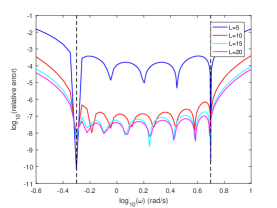
(a) $M=L$

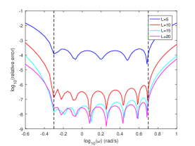
(b) $M=2L$

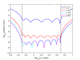
(c) $M=3L$

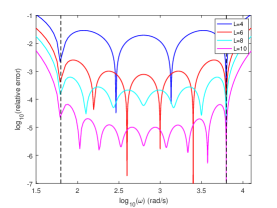
(d) $M=L$

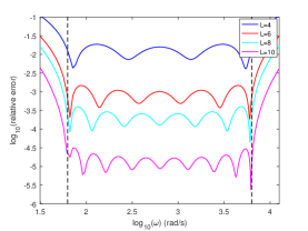
(e) $M=2L$

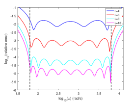
(f) $M=3L$

Figure 1: Relative errors of the square system ($M=L$) and overdetermined system ($M>L$), (a)-(c): results for $[0.5,\,5]$, (d)-(f): results for $[20\pi,\,2000\pi]$.

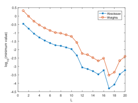
(a) $\alpha=0.3$

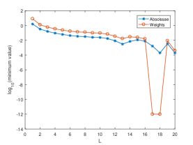
(b) $\alpha=0.5$

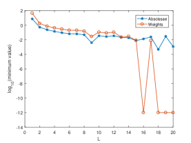
(c) $\alpha=0.7$

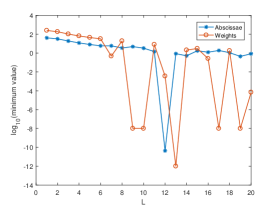
(d) $\alpha=0.3$

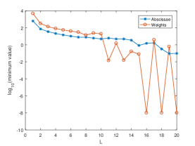
(e) $\alpha=0.5$

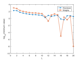
(f) $\alpha=0.7$

Figure 2: Positivity of weights ($\zeta_{\ell}$) and abscissae ($\lambda_{\ell}$) with varying $\alpha$ and $L$, (a)-(c): results for $[0.5,\,5]$, (d)-(f): results for $[20\pi,\,2000\pi]$.

6 Dispersion analysis

In this section, we present the dispersion analysis of the Cole-Cole model (2)-(4) and the approximate (55)-(58), where the external source is set to be zero. For this purpose, we assume that the magnetic field $H$, electric field $E$ and polarization field $P$ have the plane wave form

$$H = H_{0}\exp\left(i(k\,x-\omega t)\right),$$

$$E = E_{0}\exp\left(i({k}\,x-\omega t)\right),$$

$$P = P_{0}\exp\left(i({k}\,x-\omega t)\right),$$

where $E_{0},\,H_{0},\,P_{0}$ are the constant amplitudes, $\omega$ the angular frequency, and $k$ is the wave number. Injecting $H$ and $E$ into (2) gives

$$-\omega\mu_{0}H_{0}=kE_{0},$$ (68)

Substituting $H,\,E,\,P$ to (3) leads to

$$-\omega\epsilon_{0}\epsilon_{\infty}E_{0}=kH_{0}+\omega P_{0}.$$ (69)

According to the polarization equation (4), we have

$$\left(1+\mathcal{Q}(\omega)\right)P_{0}=\epsilon_{0}\left(\epsilon_{s}-\epsilon_{\infty}\right)E_{0},\quad\mathcal{Q}(\omega)=(i\omega\tau_{0})^{\alpha}.$$ (70)

Combining (68)-(70), we have

$$k^{2}=\left(\mu_{0}\epsilon_{0}\epsilon_{\infty}+\frac{\mu_{0}\epsilon_{0}\left(\epsilon_{s}-\epsilon_{\infty}\right)}{1+\mathcal{Q}(\omega)}\right)\omega^{2}.$$ (71)

In the above equation, if we replace $\mathcal{Q}(\omega)$ by

$$\mathcal{Q}^{\sharp}(\omega)=\tau_{0}^{\alpha}\frac{\sin(\pi\alpha)}{\pi}i\omega\sum_{\ell=1}^{L}\frac{\zeta_{\ell}\lambda_{\ell}^{\alpha-1}}{i\omega+\lambda_{\ell}},$$

we can obtain the dispersion relations of the approximate system (55)-(58).

With the wave modes given by (71), we deduce the phase velocities $c=\omega/\Re(k)$ and derive the attenuations $\eta=-\Im(k)$, where $\Re{k}$ and $\Im{k}$ are the real and imaginary parts of $k$, respectively. In Fig. 3, we illustrate the influence of $\alpha$ on the phase velocity and the attenuation, with the parameters $\tau_{0}=\mu_{0}=\epsilon_{0}=\epsilon_{p}=\epsilon_{\infty}=1$. Note that the case of $\alpha=1$ corresponds to the Debye model. In addition, we use the same setting to demonstrate the dispersion relations of the approximate system (55)-(58). In Fig. 4, we present the comparison of the phase velocities and attenuations obtained from the exact $\mathcal{Q}(\omega)$ and the approximate $\mathcal{Q}^{\sharp}(\omega)$; it shows an excellent agreement between the exact and approximate results. Here the weights $\zeta_{\ell}$ and abscissae $\lambda_{\ell}$ are obtain by the non-linear optimization process (section 5) with $[20\,\pi,\,200\,\pi]$ and $L=6$.

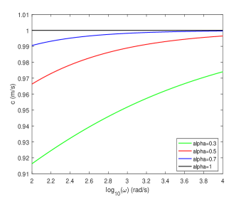
(a) phase velocity

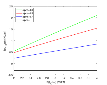
(b) attenuation

Figure 3: Dispersion relations of the Cole-Cole model (2)-(4) with varying $\alpha=0.3,\,0.5,\,0.7,\,1$.

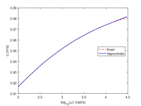
(a) $\alpha=0.3$

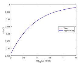
(b) $\alpha=0.5$

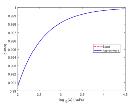
(c) $\alpha=0.7$

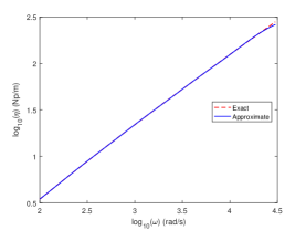
(d) $\alpha=0.3$

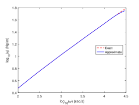
(e) $\alpha=0.5$

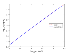
(f) $\alpha=0.7$

Figure 4: Dispersion relations of the approximate Cole-Cole model (55)-(58) with varying $\alpha=0.3,\,0.5,\,0.7$, (a)-(c): phase velocity, (d)-(f): attenuation.

7 Numerical examples

In this section, numerical examples are presented to demonstrate the accuracy of the proposed algorithm. For simplicity, we set $\tau_{0}=\mu_{0}=\epsilon_{0}\epsilon_{\infty}=\epsilon_{0}(\epsilon_{s}-\epsilon_{\infty})=1$. To our best knowledge, the regularity theory of the solutions to (2)-(6) with zero external sources is still open. The source terms $F_{i},\,i=1,2,3$ are added to assume that the exact solutions are sufficiently smooth and $P(x,t)$ have many vanishing derivatives at the initial time. The time discretization is achieved by BDF2 formula. More precisely, given initial data $U^{0},\,U^{1}$ with $U=H,\,E,\,P$, we have from the auxiliary equation (58)

$$C_{1}\psi_{\ell}^{n}+C_{2}\psi_{\ell}^{n-1}+C_{3}\psi_{\ell}^{n-2}=-\lambda_{\ell}\psi_{\ell}^{n}+C_{\alpha}\lambda_{\ell}^{\alpha-1}\left(C_{1}P^{n}+C_{2}P^{n-1}+C_{3}P^{n-2}\right),$$

or equivalently

$$\psi_{\ell}^{n}=\frac{C_{\alpha}}{C_{1}+\lambda_{\ell}}\lambda_{\ell}^{\alpha-1}\left(C_{1}P^{n}+C_{2}P^{n-1}+C_{3}P^{n-2}\right)-\frac{C_{\alpha}}{C_{1}+\lambda_{\ell}}\left(C_{2}\psi_{\ell}^{n-1}+C_{3}\psi_{\ell}^{n-2}\right),$$

where we have set

$$C_{1}=\frac{3}{2\tau},\quad C_{2}=-\frac{2}{\tau},\quad C_{3}=\frac{1}{2\tau},\quad C_{\alpha}=\frac{\sin(\pi\alpha)}{\pi}.$$

Injecting $\psi_{\ell}^{n}$ into (57), we derive

$$\left(1+\tau_{0}^{\alpha}C_{1}C_{\alpha}\sum_{\ell=1}^{L}\frac{\zeta_{\ell}\lambda_{\ell}^{\alpha-1}}{C_{1}+\lambda_{\ell}}\right)P^{n}= E^{n}-\tau_{0}^{\alpha}C_{\alpha}\sum_{\ell=1}^{L}\frac{\zeta_{\ell}\lambda_{\ell}^{\alpha-1}}{C_{1}+\lambda_{\ell}}\left(C_{2}P^{n-1}+C_{3}P^{n-2}\right)$$

$$+\tau_{0}^{\alpha}\sum_{\ell=1}^{L}\frac{\zeta_{\ell}}{C_{1}+\lambda_{\ell}}\left(C_{2}\psi_{\ell}^{n-1}+C_{3}\psi_{\ell}^{n-2}\right).$$

Using the standard BDF2 formula for (55) and (56) and combining $P^{n}$ give the computation scheme. The first initial data are set to be $U_{0},\,U=H,\,E,\,P$ and the second initial data are obtained by using forward Euler formula to (55)-(58).

7.1 Accuracy test with two external sources

As the first example, we aim to demonstrate the convergence rates of the DG scheme. For this purpose, we consider the case of $F_{3}=0$ and

$$F_{1} = \pi\sin(\pi x)\left(\frac{2\,t^{2-\alpha}}{\Gamma(1-\alpha)(1-\alpha)(2-\alpha)}+t^{2}\right)+2\pi\left(2\cos(\pi x)+\sin(\pi x)\right)\,t,$$

$$F_{2} = \cos(\pi x)\left(\frac{2\,t^{1-\alpha}}{\Gamma(1-\alpha)(1-\alpha)}+4\,t\right)-\pi^{2}\left(-2\sin(\pi x)+\cos(\pi x)\right)\,t^{2}.$$

For this case, it can be checked that (2)-(4) are satisfied by the following exact solution

$$E(x,t) = \cos(\pi x)\left(\frac{2\,t^{2-\alpha}}{\Gamma(1-\alpha)(1-\alpha)(2-\alpha)}+t^{2}\right),$$

$$H(x,t) = \pi\,(2\cos(\pi x)+\sin(\pi x))\,t^{2},$$

$$P(x,t) = \cos(\pi x)\,t^{2}.$$

The initial data are obtained by setting $t=0$ of the exact solutions and the periodic boundary condition is used. The computation domain is $\Omega=[0,\,2]$ and the total simulation time is $T=2$. The frequency band is $[0.5,\,5]$ and the number of quadrature points is $L=20$. Moreover, we set $\tau=h^{2}$ for both $\mathbb{P}^{1}$ and $\mathbb{P}^{2}$ elements such that the temporal discretization error can be relatively negligible. In Tables 1-3, we report the spatial errors in the $L^{2}$-norm and convergence orders with varying $\alpha$. The expected rates of second order for $\mathbb{P}^{1}$ elements and third order for $\mathbb{P}^{2}$ elements are reached, which confirm the optimal accuracy order of the proposed scheme.

	$N_{x}$	E			H			P
		Error	Order		Error	Order		Error	Order
$\mathbb{P}^{1}$	10	1.403E-1	–		5.118E-1	–		6.784E-2	–
	20	3.455E-2	2.022		1.220E-1	2.069		1.678E-2	2.015
	40	8.553E-3	2.014		2.972E-2	2.037		4.157E-3	2.013
	80	2.127E-3	2.008		7.330E-3	2.020		1.034E-3	2.007
$\mathbb{P}^{2}$	10	2.834E-2	–		6.605E-3	–		1.353E-2	–
	20	3.605E-3	2.975		8.868E-4	2.897		1.727E-3	2.970
	40	4.535E-4	2.991		1.172E-4	2.920		2.178E-4	2.987
	80	5.682E-5	2.997		1.522E-5	2.945		2.728E-5	2.997

Table 1: The $L^{2}$ errors and convergence orders of E, H, P for Example 7.1 with $\alpha=0.3$.

	$N_{x}$	E			H			P
		Error	Order		Error	Order		Error	Order
$\mathbb{P}^{1}$	10	1.405E-1	–		5.110E-1	–		6.722E-2	–
	20	3.470E-2	2.018		1.219E-1	2.068		1.670E-2	2.009
	40	8.621E-3	2.009		2.972E-2	2.036		4.148E-3	2.009
	80	2.151E-3	2.003		7.335E-3	2.019		1.033E-3	2.006
$\mathbb{P}^{2}$	10	2.852E-2	–		5.938E-3	–		1.310E-2	–
	20	3.645E-3	2.968		7.834E-4	2.922		1.681E-3	2.962
	40	4.599E-4	2.987		1.019E-4	2.943		2.124E-4	2.985
	80	5.774E-5	2.994		1.312E-5	2.957		2.654E-5	3.000

Table 2: The $L^{2}$ errors and convergence orders of E, H, P for Example 7.1 with $\alpha=0.5$.

	$N_{x}$	E			H			P
		Error	Order		Error	Order		Error	Order
$\mathbb{P}^{1}$	10	1.394E-1	–		5.100E-1	–		6.669E-2	–
	20	3.454E-2	2.013		1.218E-1	2.066		1.662E-2	2.005
	40	8.628E-3	2.001		2.973E-2	2.035		4.133E-3	2.008
	80	2.167E-3	1.993		7.341E-3	2.018		1.028E-3	2.007
$\mathbb{P}^{2}$	10	2.879E-2	–		5.601E-3	–		1.266E-2	–
	20	3.712E-3	2.955		7.000E-4	3.000		1.626E-3	2.961
	40	4.745E-4	2.968		8.365E-5	3.065		2.042E-4	2.993
	80	6.082E-5	2.964		1.043E-5	3.004		2.423E-5	3.075

Table 3: The $L^{2}$ errors and convergence orders of E, H, P for Example 7.1 with $\alpha=0.7$.

In order to test the efficiency of the proposed scheme, for comparison, we also implement the following scheme Li et al. (2011) to discretize the fractional derivative

$$\frac{\partial^{\alpha}\,P(x,\,t_{n})}{\partial t^{\alpha}} = a_{0}\,P^{n}(x)+\sum_{m=1}^{n-1}\left(a_{n-m}-a_{n-m-1}\right)P^{m}(x)+\mathcal{O}(\tau^{\frac{3}{2}}),$$ (72)

$$a_{m} = \frac{\tau^{-\alpha}}{\Gamma(2-\alpha)}\left[\left(m+1\right)^{1-\alpha}-m^{1-\alpha}\right],$$

where $\tau$ is the time step. We fix $\alpha=0.5$ and compare the CPU time between our fast algorithm and the direct scheme (72). The linear complexity and a significant reduction of the CPU time by our fast algorithm are observed in Fig. 5, where the number of spatial cells is fixed to be $Nx=10$ and the numbers of time steps are $Nt=10000,\,20000,\,40000,\,80000,\,160000$.

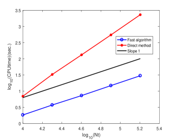
Figure 5: The CPU time with fixed $Nx=10$ and different $Nt$ for Example 7.1.

7.2 Energy analysis

The purpose of this example is to illustrate the energy properties of the Cole-Cole model (2)-(4). To this end, we use $\mathbb{P}^{1}$ elements to solve the approximate system (55)-(58) with zero external force terms and periodic boundary condition and the following initial data

$$E_{0}(x) = \cos(\pi x)\sin(\pi x),$$

$$H_{0}(x) = 2\pi\cos(\pi x)+\pi\sin(\pi x),$$

$$P_{0}(x) = 0.$$

The computation domain is $\Omega=[0,\,2]$, which is partitioned by $800$ uniform elements. The total simulation time is $T=2.5$ and the time step is set to be $\tau=h$. The weights $\zeta_{\ell}$ and abscissae $\lambda_{\ell}$ are obtained by taking $L=20$ with frequency range $[0.5,\,5]$. Fig. 6 demonstrates the energy behaviors with respect to the evolution time, where different fractional orders of $\alpha=0.3,\,0.5,\,0.7$ are considered. Since the coefficients are constant in this example, the classical energy $\tilde{\mathcal{E}}$ defined in (15) and $\mathcal{E}_{1}(=\mathcal{E}_{1}^{\sharp})$ differ only by a constant factor. Therefore the behavior of $\mathcal{E}_{1}^{\sharp}$ is the same as that of $\tilde{\mathcal{E}}$. Numerical results shown in Fig. 6 are summarized below.

• As is indicated by the blue curves in Fig. 6 (d)-(f), the energy $\mathcal{E}^{\sharp}$ is monotonically decreasing in the sense that $\mathcal{E}^{\sharp}(t_{n})-\mathcal{E}^{\sharp}(t_{n+1})>0$ for all $n$. This is consistent with Theorem 2.1.

• The nonlinear constraint optimization project preserves the positivity of the diffusive energy $\mathcal{E}^{\sharp}_{2}(t)$ given in (59) and the total energy $\mathcal{E}^{\sharp}$ given in (60), which can be seen from the red and blue curves in Fig. 6 (a)-(c). Hence the approximate system (55)-(58) is stable by Theorem 4.1.

• As is demonstrated by the green curves in Fig. 6 (a)-(c), the classical energy function defined in (19) satisfies $\widetilde{\mathcal{E}}(t_{n})<\widetilde{\mathcal{E}}(t_{0})$; this is consistent with Lemma 2.1 in Li et al. (2011). However, as can be observed from the green curves in Fig. 6 (d)-(f), the classical energy $\widetilde{\mathcal{E}}(t)$ is not a monotonically decreasing function because $\mathcal{E}_{1}(t_{n})-\mathcal{E}_{1}(t_{n+1})<0$ for some $n$. This ’non-decreasing’ phenomenon has also been reported in Huang & Wang (2019) and Bai & Rui (2022).

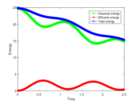
(a) $\alpha=0.3$

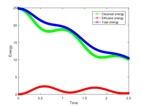
(b) $\alpha=0.5$

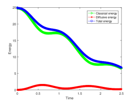
(c) $\alpha=0.7$

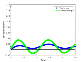
(d) $\alpha=0.3$

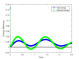
(e) $\alpha=0.5$

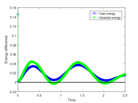
(f) $\alpha=0.7$

Figure 6: The energy behaviors of the Cole-Cole model with different fractional orders $\alpha$. In the legend, the Classical energy refers to $\mathcal{E}_{1}$, the Diffusive energy to $\mathcal{E}^{\sharp}_{2}$, the Total energy to $\mathcal{E}^{\sharp}$ and the Energy difference refers to ${\mathcal{F}}(t_{n})-{\mathcal{F}}(t_{n+1})$ with ${\mathcal{F}}=\mathcal{E}^{\sharp},\,\mathcal{E}_{1}$.

8 Conclusions

In this work, we develop a fast algorithm to solve the one-dimensional time-domain Maxwell’s equations for the Cole-Cole dispersive medium. A new, sharpened and monotonically decreasing total energy function for the Cole-Cole model is derived for the first time, which better describes the energy of a Cole-Cole medium than the classical energy defined in Li et al. (2011).

The numerical challenge imposed by the fractional derivative involved in the polarization equation is tackled by using the diffusive representation, and suitably chosen quadrature formula. A finite number of continuous auxiliary variables are introduced to approximate and localize the convolution kernel, which satisfy the local-in-time ODEs and can be easily solved.

The stability of the resulted approximate system is proved to hold as long as all the quadrature coefficients are positive. Therefore, we establish a nonlinear constrained optimization numerical scheme to preserve the positivity of the quadrature coefficients.

The spatial discretization is achieved by the DG method and we presented a rigorous error analysis for the semi-discrete DG scheme for the constant coefficient case. Compared with the convergence rate $\mathcal{O}\left(h^{k+0.5}\right)$ in Wang et al. (2021), we obtained an optimal convergence rate of $\mathcal{O}(h^{k+1})$ by a special choice of the numerical fluxes and projections. The time discretization for the approximated system is achieved by the standard BDF2 formula and the overall complexity for the proposed algorithm is $\mathcal{O}(N\,\text{log}N)$ with N being the total time steps.

References

• Bai & Rui (2022) Bai, X. & Rui, H. (2022) A second-order space-time accurate scheme for Maxwell’s equations in a Cole–Cole dispersive medium. Engineering with Computers, 1–20.
• Banks et al. (2009) Banks, H., Bokil, V. & Gibson, N. (2009) Analysis of stability and dispersion in a finite element method for Debye and Lorentz media. Numer. Meth. Part. Differ. Equ., 25, 885–917.
• Birk & Song (2010) Birk, C. & Song, C. (2010) An improved non-classical method for the solution of fractional differential equations. Comput. Mech., 46, 721–734.
• Blanc et al. (2014) Blanc, E., Chiavassa, G. & Lombard, B. (2014) Wave simulation in 2D heterogeneous transversely isotropic porous media with fractional attenuation: a Cartesian grid approach. Journal of Computational Physics, 275, 118–142.
• Bo et al. (2014) Bo, W., Ziqing, X. & Zhang, Z. (2014) Space-time discontinuous Galerkin method for Maxwell equations in dispersive media. Acta Math. Sci., 34, 1357–1376.
• Bokil et al. (2017) Bokil, V. A., Cheng, Y., Jiang, Y. & Li, F. (2017) Energy stable discontinuous Galerkin methods for Maxwell’s equations in nonlinear optical media. J. Comput. Phys., 350, 420–452.
• Cassier et al. (2017) Cassier, M., Joly, P. & Kachanovska, M. (2017) Mathematical models for dispersive electromagnetic waves: an overview. Comput. Math. Appl., 74, 27922830.
• Causley et al. (2011) Causley, M. F., Petropoulos, P. G. & Jiang, S. (2011) Incorporating the Havriliak–Negami dielectric model in the FD-TD method. J. Comput. Phys., 230, 3884–3899.
• Ciarlet (2002) Ciarlet, P. G. (2002) The finite element method for elliptic problems. SIAM.
• Cockburn et al. (2004) Cockburn, B., Li, F. & Shu, C.-W. (2004) Locally divergence-free discontinuous Galerkin methods for the Maxwell equations. J. Comput. Phys., 194, 588–610.
• Cole & Cole (1941) Cole, K. S. & Cole, R. H. (1941) Dispersion and absorption in dielectrics I. Alternating current characteristics. J. Chem. phys., 9, 341–351.
• Debye (1929) Debye, P. J. W. (1929) Polar molecules. Dover publications.
• Desch & Miller (1988) Desch, W. & Miller, R. (1988) Exponential stabilization of Volterra integral equations with singular kernels. J. Integral Equations Appl., 3, 397–433.
• Diethelm (2008) Diethelm, K. (2008) An investigation of some nonclassical methods for the numerical approximation of Caputo-type fractional derivatives. Numer. Algorithms, 47, 361–390.
• Gabriel et al. (1996) Gabriel, S., Lau, R. & Gabriel, C. (1996) The dielectric properties of biological tissues: III. Parametric models for the dielectric spectrum of tissues. Phys. Med. & Biol., 41, 2271.
• Garrappa et al. (2016) Garrappa, R., Mainardi, F. & Maione, G. (2016) Models of dielectric relaxation based on completely monotone functions. Fract. Calc. Appl. Anal., 19, 1105–1160.
• Guo et al. (2006) Guo, B., Li, J. & Zmuda, H. (2006) A new FDTD formulation for wave propagation in biological media with Cole–Cole model. IEEE Microw. Wirel. Compon. Lett., 16, 633–635.
• Haddar et al. (2010) Haddar, H., Li, J.-R. & Matignon, D. (2010) Efficient solution of a wave equation with fractional-order dissipative terms. Journal of Computational and Applied Mathematics, 234, 2003–2010.
• Havriliak & Negami (1967) Havriliak, S. & Negami, S. (1967) A complex plane representation of dielectric and mechanical relaxation processes in some polymers. Polymer, 8, 161–210.
• Hesthaven & Warburton (2002) Hesthaven, J. S. & Warburton, T. (2002) Nodal high-order methods on unstructured grids: I. time-domain solution of maxwell’s equations. J. Comput. Phys., 181, 186–221.
• Hoekstra & Delaney (1974) Hoekstra, P. & Delaney, A. (1974) Dielectric properties of soils at UHF and microwave frequencies. J. Geophys. Res., 79, 1699–1708.
• Huang & Wang (2019) Huang, C. & Wang, L.-L. (2019) An accurate spectral method for the transverse magnetic mode of Maxwell equations in Cole-Cole dispersive media. Adv. Comput. Math., 45, 707–734.
• Huang et al. (2011) Huang, Y., Li, J. & Yang, W. (2011) Interior penalty DG methods for Maxwell’s equations in dispersive media. J. Comput. Phys., 230, 4559–4570.
• Jiao & Jin (2001) Jiao, D. & Jin, J.-M. (2001) Time-domain finite element modeling of dispersive media. IEEE Antennas and Propagation Society International Symposium., vol. 3. IEEE, IEEE, pp. 180–183.
• Kappel & Kuntsevich (2000) Kappel, F. & Kuntsevich, A. (2000) An implementation of Shor’s r-algorithm. Comput. Optim. Appl., 15, 193–205.
• Li et al. (2011) Li, J., Huang, Y. & Lin, Y. (2011) Developing finite element methods for Maxwell’s equations in a Cole–Cole dispersive medium. SIAM J. Sci. Comput., 33, 3153–3174.
• Li & Chen (2006) Li, J. & Chen, Y. (2006) Analysis of a time-domain finite element method for 3-D Maxwell’s equations in dispersive media. Comput. Meth. Appl. Mech. Eng., 195, 4220–4229.
• Lombard & Matignon (2016) Lombard, B. & Matignon, D. (2016) Diffusive approximation of a time-fractional Burger’s equation in nonlinear acoustics. SIAM J. Appl. Math., 76, 1765–1791.
• Lu et al. (2004) Lu, T., Zhang, P. & Cai, W. (2004) Discontinuous Galerkin methods for dispersive and lossy Maxwell’s equations and PML boundary conditions. J. Comput. Phys., 200, 549–580.
• Luebbers & Hunsberger (1992) Luebbers, R. J. & Hunsberger, F. (1992) FDTD for Nth-order dispersive media. IEEE Trans. Antennas Propag., 40, 1297–1301.
• Lyu et al. (2020) Lyu, M., Chew, W. C., Jiang, L., Li, M. & Xu, L. (2020) Numerical simulation of a coupled system of Maxwell equations and a gas dynamic model. J. Comput. Phys., 409, 109354.
• McDonald (2019) McDonald, K. T. (2019) Electrodynamics in 1 and 2 spatial dimensions. https://www.physics.princeton.edu/ mcdonald/examples/2dem.pdf.
• Mrozowski & Stuchly (1997) Mrozowski, M. & Stuchly, M. A. (1997) Parameterization of media dispersive properties for FDTD. IEEE Trans. Antennas Propag., 45, 1438–1439.
• Podlubny (1999) Podlubny, I. (1999) Fractional differential equations : an introduction to fractional derivatives, fractional differential equations, to methods of their solution and some of their applications. Academic Press.
• Polk & Postow (1995) Polk, C. & Postow, E. (1995) Handbook of Biological Effects of Electromagnetic Fields, -2 Volume Set. CRC press.
• Rekanos (2011) Rekanos, I. T. (2011) FDTD schemes for wave propagation in Davidson-Cole dispersive media using auxiliary differential equations. IEEE Trans. Antennas Propag., 60, 1467–1478.
• Rekanos & Papadopoulos (2010) Rekanos, I. T. & Papadopoulos, T. G. (2010) An auxiliary differential equation method for FDTD modeling of wave propagation in Cole-Cole dispersive media. IEEE Trans. Antennas Propag., 58, 3666–3674.
• Schuster & Luebbers (1998) Schuster, J. & Luebbers, R. (1998) An FDTD algorithm for transient propagation in biological tissue with a Cole-Cole dispersion relation. in: Proceedings of the IEEE Antennas and Propagation Society Int. Symp., 4, 1988–1991.
• Shor (1985) Shor, N. (1985) Minimization methods for non-differentiable functions. Springer Ser. Comput. Math., 3.
• Torres et al. (1996) Torres, F., Vaudon, P. & Jecko, B. (1996) Application of fractional derivatives to the FDTD modeling of pulse propagation in a Cole–Cole dispersive medium. Microwave Opt. Technol. Let., 13, 300–304.
• Wang et al. (2010) Wang, B., Xie, Z. & Zhang, Z. (2010) Error analysis of a discontinuous Galerkin method for Maxwell equations in dispersive media. J. Comput. Phys., 229, 8552–8563.
• Wang et al. (2021) Wang, J., Zhang, J. & Zhang, Z. (2021) A CG–DG method for maxwell’s equations in Cole–Cole dispersive media. J. Comput. Appl. Math., 393, 113480.
• Xie et al. (2019) Xie, J., Ou, M. Y. & Xu, L. (2019) A discontinuous Galerkin method for wave propagation in orthotropic poroelastic media with memory terms. Journal of Computational Physics, 397, 108865.
• Yang et al. (2021) Yang, Y., Wang, L.-L. & Zeng, F. (2021) Analysis of a backward Euler-type scheme for Maxwell’s equations in a Havriliak–Negami dispersive medium. ESAIM: Math. Model. Numer. Anal., 55, 479–506.
• Yuan & Agrawal (2002) Yuan, L. & Agrawal, O. (2002) A numerical scheme for dynamic systems containing fractional derivatives. J. Vibr. Acoust., 124, 321–324.