UFIFT-QG-22-02

Reheating with Effective Potentials

S. Katuwal^1∗, S. P. Miao^2⋆ and R. P. Woodard^1†

¹ Department of Physics, University of Florida,
Gainesville, FL 32611, UNITED STATES

² Department of Physics, National Cheng Kung University,
No. 1 University Road, Tainan City 70101, TAIWAN

ABSTRACT

We consider reheating for a charged inflaton which is minimally coupled to electromagnetism. The evolution of such an inflaton induces a time-dependent mass for the photon. We show how the massive photon propagator can be expressed as a spatial Fourier mode sum involving three different sorts of mode functions, just like the constant mass case. We develop accurate analytic approximations for these mode functions, and use them to approximate the effective force exerted on the inflaton $0$-mode. This effective force allows one to simply compute the evolution of the inflaton $0$-mode and to follow the progress of reheating.

PACS numbers: 04.50.Kd, 95.35.+d, 98.62.-g

^∗ e-mail: sanjib.katuwal@ufl.edu

^⋆ email: spmiao5@mail.ncku.edu.tw

^† e-mail: woodard@phys.ufl.edu

1 Introduction

Scalar-driven inflation is supported by the slow roll of the inflaton down its potential. At the end of inflation the inflaton begins oscillating, and its kinetic energy is transferred to ordinary matter during the process of reheating. The efficiency of this transfer obviously depends on the way the inflaton is coupled to ordinary matter. Ema et al. have shown that the most efficient coupling is that of a charged inflaton to electromagnetism [1].

What happens is that the evolution of a charged inflaton induces a time-dependent photon mass which oscillates around zero during reheating. The temporal and longitudinal components of the photon diverge as the mass goes to zero, which makes reheating very efficient. The process has been previously studied by discretizing space, carrying out a finite Fourier transform, and then numerically evolving the nonlinear system of the inflaton plus electromagnetism [2]. However, the energy transfer is broadly distributed over so many modes that there is little point to including nonlinear effects in the photon field, provided that its response to the inflaton $0$-mode is known to all orders. In that case, one merely sums the contribution from each photon mode’s wave vector, which can be accomplished by varying the inflaton effective potential. The goal of this paper is to develop a good analytic approximation for the massive photon propagator in a time-dependent inflaton background, and then use it to compute the quantum-induced, effective force in the equation for the inflaton $0$-mode. In this way reheating can be studied by numerically solving a nonlocal equation for the inflaton $0$-mode.

This paper consists of five sections, of which the first is this Introduction. In section 2 we derive a spatial Fourier mode sum for the massive photon propagator which is valid when the mass becomes time-dependent. Section 3 develops analytic approximations for the temporal and longitudinal modes, checking them against explicit numerical analysis for a simple model of inflation. In section 4 we discuss how these approximations can be used to estimate the quantum-induced effective force which controls the process of reheating. Section 5 gives our conclusions.

2 The Massive Photon Propagator

The purpose of this section is to generalize the massive photon propagator from its known form for a constant mass [3] to the case of a time-dependent mass. The Lagrangian is,

$$\mathcal{L}=-\frac{1}{4}F_{\mu\nu}F_{\rho\sigma}g^{\mu\rho}g^{\nu\sigma}\sqrt{-g}$$ (1)

$$\hskip 56.9055pt-\Bigl{(}\partial_{\mu}\!-\!iqA_{\mu}\Bigr{)}\varphi\Bigl{(}\partial_{\nu}\!+\!iqA_{\nu}\Bigr{)}\varphi^{*}g^{\mu\nu}\sqrt{-g}-V(\varphi\varphi^{*})\sqrt{-g}\;,\qquad$$

where $\varphi$ is the inflaton and $F_{\mu\nu}\equiv\partial_{\mu}A_{\nu}-\partial_{\nu}A_{\mu}$ is the electromagnetic field strength. We work on a general homogeneous, isotropic and spatially flat geometry in $D$-dimensional, conformal coordinates, with Hubble parameter $H$ and first slow roll parameter $\epsilon$,

$$ds^{2}=a^{2}\Bigl{[}-d\eta^{2}+d\vec{x}\!\cdot\!d\vec{x}\Bigr{]}\qquad,\qquad H\equiv\frac{\partial_{0}a}{a^{2}}\quad,\quad\epsilon\equiv-\frac{\partial_{0}H}{aH^{2}}\;.$$ (2)

The section first reviews the constant mass case, and then makes the generalizations necessary to incorporate a time-dependent mass.

2.1 Constant Mass

When the photon’s mass is constant its propagator $i[\mbox{}_{\mu}\Delta_{\rho}](x;x^{\prime})$ is transverse,

$$\partial_{\mu}\Bigl{\{}\!\sqrt{-g(x)}\,g^{\mu\nu}(x)\,i\Bigl{[}\mbox{}_{\nu}\Delta_{\rho}\Bigr{]}(x;x^{\prime})\Bigr{\}}=0=\partial^{\prime}_{\rho}\Bigl{\{}\!\sqrt{-g(x^{\prime})}\,g^{\rho\sigma}(x^{\prime})\,i\Bigl{[}\mbox{}_{\mu}\Delta_{\sigma}\Bigr{]}(x;x^{\prime})\Bigr{\}}.$$ (3)

Its propagator equation reflects this transversality [3, 4],

$$\sqrt{-g}\Bigl{[}\kern 1.0pt\vbox{\hrule height=1.2pt\hbox{\vrule width=1.2pt\hskip 3.0pt\vbox{\vskip 6.0pt}\hskip 3.0pt\vrule width=0.6pt}\hrule height=0.6pt}\kern 1.0pt^{\mu\nu}-R^{\mu\nu}-M^{2}g^{\mu\nu}\Bigr{]}i\Bigl{[}\mbox{}_{\nu}\Delta_{\rho}\Bigr{]}(x;x^{\prime})$$ (4)

$$\hskip 99.58464pt=\delta^{\mu}_{~{}\rho}i\delta^{D}(x\!-\!x^{\prime})+\sqrt{-g(x)}\,g^{\mu\nu}(x)\partial_{\nu}\partial^{\prime}_{\rho}i\Delta(x;x^{\prime})\;.\qquad$$

Here $\kern 1.0pt\vbox{\hrule height=1.2pt\hbox{\vrule width=1.2pt\hskip 3.0pt\vbox{\vskip 6.0pt}\hskip 3.0pt\vrule width=0.6pt}\hrule height=0.6pt}\kern 1.0pt^{\mu\nu}$ is the vector d’Alembertian, $R^{\mu\nu}$ is the Ricci tensor and $i\Delta(x;x^{\prime})$ is the propagator of a massless, minimally coupled scalar,

$$\partial_{\mu}\Bigl{[}\sqrt{-g}\,g^{\mu\nu}\partial_{\nu}i\Delta(x;x^{\prime})\Bigr{]}=i\delta^{D}(x\!-\!x^{\prime})\;.$$ (5)

The solution to (3-4) can be expressed as a spatial Fourier mode sum over three sorts of polarizations [3],

$$i\Bigl{[}\mbox{}_{\mu}\Delta_{\rho}\Bigr{]}(x;x^{\prime})=\int\!\!\frac{d^{D-1}k}{(2\pi)^{D-1}}\sum_{\lambda=t,u,v}s_{\lambda}\Biggl{\{}\theta(\Delta\eta)\mathcal{A}_{\mu}(x;\vec{k},\lambda)\mathcal{A}_{\nu}^{*}(x^{\prime};\vec{k},\lambda)$$ (6)

$$\hskip 170.71652pt+\theta(-\Delta\eta)\mathcal{A}_{\mu}^{*}(x;\vec{k},\lambda)\mathcal{A}_{\nu}(x^{\prime};\vec{k},\lambda)\Biggr{\}},\qquad$$

where $\Delta\eta\equiv\eta-\eta^{\prime}$. Longitudinal photons correspond to $\lambda=t$ and have $s_{t}=-1$ with,

$$\mathcal{A}_{\mu}(x;\vec{k},t)=\frac{\partial_{\mu}}{M}\Bigl{[}t(\eta,k)e^{i\vec{k}\cdot\vec{x}}\Bigr{]}\;\;,\;\;\Bigl{[}\mathcal{D}\partial_{0}+k^{2}\Bigr{]}t=0\;\;,\;\;t\cdot\partial_{0}t^{*}-\partial_{0}t\cdot t^{*}=\frac{i}{a^{D-2}},$$ (7)

where $\mathcal{D}\equiv\partial_{0}+(D-2)aH$. Temporal photons correspond to $\lambda=u$ and have $s_{u}=+1$ with,

$$\mathcal{A}_{\mu}(x;\vec{k},u)=\frac{\overline{\partial}_{\mu}}{M}\Bigl{[}u(\eta,k)e^{i\vec{k}\cdot\vec{x}}\Bigr{]} \overline{\partial}_{0}\equiv k\;\;,\;\;\overline{\partial}_{m}\equiv\frac{-ik_{m}}{k}\mathcal{D}\;,\qquad$$ , (8)

$$\Bigl{[}\partial_{0}\mathcal{D}+k^{2}+a^{2}M^{2}\Bigr{]}u=0 u\cdot\partial_{0}u^{*}-\partial_{0}u\cdot u^{*}=\frac{i}{a^{D-2}}.\qquad$$ , (9)

Transverse spatial photons correspond to $\lambda=v$ and have $s_{v}=+1$ with,

$$\mathcal{A}_{\mu}(x;\vec{k},v)=\epsilon_{\mu}(\vec{k},v)\,v(\eta,k)e^{i\vec{k}\cdot\vec{x}} \epsilon_{0}=0\;\;,\;\;k_{m}\epsilon_{m}=0\;,\qquad$$ , (10)

$$\Bigl{[}\partial^{2}_{0}+(D\!-\!4)aH\partial_{0}+k^{2}+a^{2}M^{2}\Bigr{]}v=0 v\cdot\partial_{0}v^{*}-\partial_{0}v\cdot v^{*}=\frac{i}{a^{D-4}},\qquad$$ , (11)

where the sum over the $(D-2)$ spatial polarizations gives,

$$\sum_{v}\epsilon_{i}(\vec{k},v)\times\epsilon^{*}_{j}(\vec{k},v)=\delta_{ij}-\frac{k_{i}k_{j}}{k^{2}}\;.$$ (12)

2.2 Time-Dependent Mass

To understand the case of a time-dependent mass we must consider the vector and scalar field equations,

$$\frac{\delta S}{\delta A_{\mu}}=\partial_{\nu}\Bigl{[}\sqrt{-g}\,g^{\nu\rho}g^{\mu\sigma}F_{\rho\sigma}\Bigr{]}$$ (13)

$$\hskip 71.13188pt+iq\Bigl{[}\varphi\!\cdot\!\Bigl{(}\partial_{\nu}\!+\!iqA_{\nu}\Bigr{)}\varphi^{*}-\Bigl{(}\partial_{\nu}\!-\!iqA_{\nu}\Bigr{)}\varphi\!\cdot\!\varphi^{*}\Bigr{]}g^{\mu\nu}\sqrt{-g}\;,\qquad$$

$$\frac{\delta S}{\delta\varphi^{*}}=\Bigl{(}\partial_{\mu}\!-\!iqA_{\mu}\Bigr{)}\Bigl{[}\sqrt{-g}\,g^{\mu\nu}\Bigl{(}\partial_{\nu}\!-\!iqA_{\nu}\Bigr{)}\varphi\Bigr{]}-\varphi V^{\prime}(\varphi\varphi^{*})\sqrt{-g}\;.$$ (14)

The $0$-th order inflaton is $\varphi_{0}(\eta)$ which is real and obeys the equation,

$$\partial_{0}\Bigl{[}a^{D-2}\partial_{0}\varphi_{0}\Bigr{]}+a^{D}\varphi_{0}V^{\prime}(\varphi_{0}^{2})=0\;.$$ (15)

The first order perturbations are $A_{\mu}(x)$ and the real fields $\alpha(x)$ and $\beta(x)$,

$$\varphi(x)=\varphi_{0}(\eta)+\alpha(x)+i\beta(x)\;.$$ (16)

The first order contribution to the vector equation (13) is,

$$\partial_{\nu}\Bigl{[}\sqrt{-g}\,g^{\nu\rho}g^{\mu\sigma}F_{\rho\sigma}\Bigr{]}-2q^{2}\varphi_{0}^{2}\Bigl{[}A_{\nu}-\partial_{\nu}\Bigl{(}\frac{\beta}{q\varphi_{0}}\Bigr{)}\Bigr{]}\sqrt{-g}\,g^{\nu\mu}=0\;.$$ (17)

The photon mass is $M^{2}\equiv 2q^{2}\varphi_{0}^{2}$. Note from equation (17) that antisymmetry of the field strength tensor implies,

$$\partial_{\mu}\Bigl{[}M^{2}\sqrt{-g}\,g^{\mu\nu}\Bigl{(}A_{\nu}-\partial_{\nu}\Bigl{(}\frac{\beta}{q\varphi_{0}}\Bigr{)}\Bigr{]}=0\;.$$ (18)

This constraint is identical to the imaginary part of the first order contribution to the scalar equation (14). The analogous real part is,

$$\partial_{\mu}\Bigl{[}\sqrt{-g}\,g^{\mu\nu}\partial_{\nu}\alpha\Bigr{]}-\sqrt{-g}\Bigl{[}V^{\prime}(\varphi_{0}^{2})+2\varphi_{0}^{2}V^{\prime\prime}(\varphi_{0}^{2})\Bigr{]}\alpha=0\;.$$ (19)

Relations (17) and (18) demonstrate that the Higgs mechanism continues to function when the scalar background $\varphi_{0}$ depends upon spacetime. To simplify the subsequent analysis, we will absorb (“eat”) the imaginary part of the scalar perturbation into the vector field as usual,

$$A_{\mu}-\partial_{\mu}\Bigl{(}\frac{\beta}{q\varphi_{0}}\Bigr{)}\longrightarrow A_{\mu}\;.$$ (20)

We can also use the conformal coordinate relation $g_{\mu\nu}=a^{2}\eta_{\mu\nu}$ to provide simple expressions for (17) and (18),

$$\partial_{\nu}\Bigl{[}a^{D-4}F^{\nu\mu}\Bigr{]}-M^{2}a^{D-2}A^{\mu}=0\qquad\Longrightarrow\qquad\partial_{\mu}\Bigl{[}M^{2}a^{D-2}A^{\mu}\Bigr{]}=0\;,$$ (21)

where $F^{\nu\mu}\equiv\eta^{\nu\rho}\eta^{\mu\sigma}F_{\rho\sigma}$ and $A^{\mu}\equiv\eta^{\mu\nu}A_{\nu}$. The $3+1$ decomposition of the constraint on the right hand side of (21) is,

$$\Bigl{[}\mathcal{D}+\frac{2\partial_{0}M}{M}\Bigr{]}A_{0}-\partial_{m}A_{m}=0\qquad,\qquad\mathcal{D}\equiv\partial_{0}+(D\!-\!2)aH\;.$$ (22)

Relation (22) permits us to $3+1$ decompose the left hand side of (21) to,

$$\Bigl{[}\partial_{0}\Bigl{(}\mathcal{D}+\frac{2\partial_{0}M}{M}\Bigr{)}-\nabla^{2}+a^{2}M^{2}\Bigr{]}A_{0} \!\!\!=\!\!\! 0\;,$$ (23)

$$2\Bigl{(}aH+\frac{\partial_{0}M}{M}\Bigr{)}\partial_{m}A_{0}+\Bigl{[}\partial_{0}^{2}+(D\!-\!4)aH\partial_{0}-\nabla^{2}+a^{2}M^{2}\Bigr{]}A_{m} \!\!\!=\!\!\! 0\;.$$ (24)

Equations (22-24) are satisfied by three polarizations of spatial plane waves whose associated mode functions are $t(\eta,k)$, $u(\eta,k)$ and $v(\eta,k)$. Our notation is that a “tilde” over a differential operator such as $\partial_{0}$ or $\mathcal{D}$ indicates the addition of $\partial_{0}M/M$, whereas a “hat” denotes subtraction of the same quantity,

$$\widetilde{\mathcal{D}}\equiv\mathcal{D}+\frac{\partial_{0}M}{M}\qquad,\qquad\widehat{\partial}_{0}\equiv\partial_{0}-\frac{\partial_{0}M}{M}\;.$$ (25)

What we term Longitudinal photons have the form,

$$\mathcal{A}_{0}(x;\vec{k},t)=\frac{\widehat{\partial}_{0}t(\eta,k)}{M(\eta)}\,e^{i\vec{k}\cdot\vec{x}}\qquad,\qquad\mathcal{A}_{m}(x;\vec{k},t)=\frac{ik_{m}t(\eta,k)}{M(\eta)}\,e^{i\vec{k}\cdot\vec{x}}\;,$$ (26)

where the mode function $t(\eta,k)$ obeys,

$$\Bigl{[}\widetilde{\mathcal{D}}\widehat{\partial}_{0}+k^{2}\Bigr{]}t=0\qquad,\qquad t\cdot\partial_{0}t^{*}-\partial_{0}t\cdot t^{*}=\frac{i}{a^{D-2}}\;.$$ (27)

Temporal photons take the form,

$$\mathcal{A}_{0}(x;\vec{k},u)=\frac{ku(\eta,k)}{M(\eta)}\,e^{i\vec{k}\cdot\vec{x}}\qquad,\qquad\mathcal{A}_{m}(x;\vec{k},u)=-\frac{ik_{m}\widetilde{\mathcal{D}}u(\eta,k)}{kM(\eta)}\,e^{i\vec{k}\cdot\vec{x}}\;,$$ (28)

where the mode function $u(\eta,k)$ obeys,

$$\Bigl{[}\widehat{\partial}_{0}\widetilde{\mathcal{D}}+k^{2}+a^{2}M^{2}\Bigr{]}u=0\qquad,\qquad u\cdot\partial_{0}u^{*}-\partial_{0}u\cdot u^{*}=\frac{i}{a^{D-2}}\;.$$ (29)

The tendency for longitudinal and temporal photons to diverge when the mass $M(\eta)$ passes through zero is obvious from expressions (26) and (28). In contrast, the time-dependent mass makes no change at all in relations (10-12) for the Transverse spatial photons, and these polarizations remain finite as the mass passes through zero.

A time-dependent mass makes no change in mode sum (6) for the propagator. However, the propagator obeys a revised version of the constraint equation (3),

$$\partial^{\mu}\Bigl{\{}a^{D-2}M^{2}i\Bigl{[}\mbox{}_{\mu}\Delta_{\rho}\Bigr{]}(x;x^{\prime})\Bigr{\}}=0=\partial^{\prime\rho}\Bigl{\{}{a^{\prime}}^{D-2}{M^{\prime}}^{2}i\Bigl{[}\mbox{}_{\mu}\Delta_{\rho}\Bigr{]}(x;x^{\prime})\Bigr{\}}\;.$$ (30)

The propagator equations analogous to (4-5) can be given in terms of the massive photon kinetic operator,

$$\mathcal{D}^{\mu\nu}\equiv\partial_{\alpha}\Bigl{[}a^{D-4}\Bigl{(}\eta^{\mu\nu}\partial^{\alpha}-\eta^{\alpha\nu}\partial^{\mu}\Bigr{)}\Bigr{]}-a^{D-2}M^{2}\eta^{\mu\nu}\;.$$ (31)

The revised versions of (4-5) are,

$$\mathcal{D}^{\mu\nu}i\Bigl{[}\mbox{}_{\nu}\Delta_{\rho}\Bigr{]}(x;x^{\prime}) \!\!\!=\!\!\! \delta^{\mu}_{~{}\rho}i\delta^{D}(x\!-\!x^{\prime})+\frac{a^{D-2}M}{M^{\prime}}\widehat{\partial}^{\mu}\widehat{\partial}^{\prime}_{\rho}i\Delta_{t}(x;x^{\prime})\;,\qquad$$ (32)

$$\frac{1}{M}\partial^{\mu}\Bigl{[}a^{D-2}M\widehat{\partial}_{\mu}i\Delta_{t}(x;x^{\prime})\Bigr{]} \!\!\!=\!\!\! i\delta^{D}(x\!-\!x^{\prime})\;.\qquad$$ (33)

3 Approximating the Amplitudes

The purpose of this section is to develop analytic approximations for the crucial mode functions $t(\eta,k)$ and $u(\eta,k)$. We begin by giving a dimensionless formulation of the problem. This formalism is then employed to derive good analytic approximations for first, the longitudinal amplitude and then, the temporal amplitude. At each stage these approximations are checked against explicit numerical evolution in a simple mode of inflation.

3.1 Dimensionless Formulation

It is best to change the evolution variable from conformal time $\eta$ to the number of e-foldings from the start of inflation, $n\equiv\ln[a(\eta)]$,

$$\partial_{0}=aH\frac{\partial}{\partial n}\qquad,\qquad\partial_{0}^{2}=a^{2}H^{2}\Bigl{[}\frac{\partial^{2}}{\partial n^{2}}+(1\!-\!\epsilon)\frac{\partial}{\partial n}\Bigr{]}\;.$$ (34)

We can also use factors of $8\pi G$ to make the inflaton, the Hubble parameter and the scalar potential dimensionless,

$$\psi(n)\equiv\sqrt{8\pi G}\,\varphi_{0}(\eta)\quad,\quad\chi(n)\equiv\sqrt{8\pi G}\,H(\eta)\quad,\quad U(\psi^{2})\equiv(8\pi G)^{2}V(\varphi^{2}_{0})\;.$$ (35)

This gives dimensionless forms for the classical Friedmann equations, and for the inflaton evolution equation,

$$\frac{1}{2}(D\!-\!2)(D\!-\!1)\chi^{2} \!\!\!=\!\!\! \chi^{2}{\psi^{\prime}}^{2}+U(\psi^{2})\;,\qquad$$ (36)

$$-\frac{1}{2}(D\!-\!2)\Bigl{[}(D\!-\!1)-2\epsilon\Bigr{]}\chi^{2} \!\!\!=\!\!\! \chi^{2}{\psi^{\prime}}^{2}-U(\psi^{2})\;,\qquad$$ (37)

$$0 \!\!\!=\!\!\! \chi^{2}\Bigl{[}\psi^{\prime\prime}+(D\!-\!1\!-\!\epsilon)\psi^{\prime}\Bigr{]}+\psi U^{\prime}(\psi^{2})\;.\qquad$$ (38)

Factors of $8\pi G$ can be extracted to give similar dimensionless forms for the time-dependent mass $M^{2}(\eta)\equiv 2q^{2}\varphi_{0}^{2}(\eta)$ and the wave number $k^{2}$,

$$\mu^{2}(n)\equiv 8\pi GM^{2}(\eta)=2q^{2}\psi^{2}(n)\qquad,\qquad\kappa^{2}\equiv 8\pi Gk^{2}\;.$$ (39)

We define the dimensionless Longitudinal and Temporal amplitudes as,

$$\mathcal{T}(n,\kappa)\equiv\ln\Bigl{[}\frac{|t(\eta,k)|^{2}}{\sqrt{8\pi G}}\Bigr{]}\qquad,\qquad\mathcal{U}(n,\kappa)\equiv\ln\Bigl{[}\frac{|u(\eta,k)|^{2}}{\sqrt{8\pi G}}\Bigr{]}\;.$$ (40)

By combining the mode equations and Wronskians (27) and (29) for each mode we can infer a single nonlinear relation for the associated amplitudes [5, 6, 7],

$$\mathcal{T}^{\prime\prime}+\frac{1}{2}{\mathcal{T}^{\prime}}^{2}+(D\!-\!1\!-\!\epsilon)\mathcal{T}^{\prime}+\frac{2\kappa^{2}e^{-2n}}{\chi^{2}}+\frac{2\mu_{t}^{2}}{\chi^{2}}-\frac{e^{-2[\mathcal{T}+(D-1)n]}}{2\chi^{2}} \!\!\!=\!\!\! 0\;,\qquad$$ (41)

$$\mathcal{U}^{\prime\prime}+\frac{1}{2}{\mathcal{U}^{\prime}}^{2}+(D\!-\!1\!-\!\epsilon)\mathcal{U}^{\prime}+\frac{2\kappa^{2}e^{-2n}}{\chi^{2}}+\frac{2\mu_{u}^{2}}{\chi^{2}}-\frac{e^{-2[\mathcal{U}+(D-1)n]}}{2\chi^{2}} \!\!\!=\!\!\! 0\;,\qquad$$ (42)

where a prime denotes differentiation with respect to $n$ and the two masses are,

$$\frac{\mu^{2}_{t}}{\chi^{2}} \!\!\!\equiv\!\!\! -(D\!-\!1\!-\!\epsilon)\frac{\mu^{\prime}}{\mu}-\frac{\mu^{\prime\prime}}{\mu}\;,\qquad$$ (43)

$$\frac{\mu^{2}_{u}}{\chi^{2}} \!\!\!\equiv\!\!\! (D\!-\!2)(1\!-\!\epsilon)+\frac{\mu^{2}}{\chi^{2}}-(D\!-\!3\!+\!\epsilon)\frac{\mu^{\prime}}{\mu}+\Bigl{(}\frac{\mu^{\prime}}{\mu}\Bigr{)}^{\prime}-\Bigl{(}\frac{\mu^{\prime}}{\mu}\Bigr{)}^{2}\;.\qquad$$ (44)

Because $\mu^{2}(n)=2q^{2}\psi^{2}(n)$ we can use the inflaton $0$-mode equation (38) to simplify the $t$-mode mass,

$$\frac{\mu^{2}_{t}}{\chi^{2}}=-\frac{[\psi^{\prime\prime}+(D\!-\!1\!-\!\epsilon)\psi^{\prime}]}{\psi}=\frac{U^{\prime}(\psi^{2})}{\chi^{2}}\;.$$ (45)

In order to follow the amplitudes numerically one must use a specific model of inflation. For simplicity we have chosen the quadratic mass model, $U=c^{2}\psi^{2}$, even though its prediction for the tensor-to-scalar ratio is disfavored by the data [8, 9]. The Slow Roll Approximation gives analytic expressions for this model which are accurate until almost the end of inflation,

$$\psi(n)\simeq\sqrt{\psi_{0}^{2}\!-\!2n}\quad,\quad\chi(n)\simeq\frac{c}{\sqrt{3}}\sqrt{\psi_{0}^{2}\!-\!2n}\quad,\quad\epsilon(n)\simeq\frac{1}{\psi_{0}^{2}\!-\!2n}\;,$$ (46)

where $\psi_{0}$ is the initial value of the dimensionless inflaton $0$-mode. About 56 e-foldings of inflation results from the choice $\psi_{0}=10.6$. To estimate the constant $c$, note that modes which experience 1st horizon crossing at e-folding $n_{1}$ (that is, $\kappa=\chi(n_{1})e^{n_{1}}$) have the following approximate scalar power spectrum and spectral index,

$$\Delta^{2}_{\mathcal{R}}(n_{1})\simeq\frac{1}{8\pi^{2}}\frac{\chi^{2}(n_{1})}{\epsilon(n_{1})}\qquad\Longrightarrow\qquad 1-n_{s}\simeq 2\epsilon+\frac{\epsilon^{\prime}}{\epsilon}\;.$$ (47)

Hence the observed scalar spectral index is consistent with $\psi_{0}=10.6$, and the observed scalar amplitude with the choice of $c=7.1\times 10^{-6}$ [8, 9]. We must also choose a specific value for the charge $q$. Using $q^{2}=1/137$ would cause the classical potential of $U=c^{2}\psi^{2}$ to be completely overwhelmed by the 1-loop Coleman-Weinberg correction of $\Delta U\simeq 3/64\pi^{2}\times\mu^{4}\ln(\mu^{2}/s^{2})$, where $s$ is the dimensionless renormalization scale [10]. Choosing the much smaller value of $q=1.2\times 10^{-6}$ reduces the 1-loop correction to a negligible tenth of a percent effect at the start of inflation.

Once we have a specific model it is possible to understand the magnitudes of the various terms. Figure 1 shows the dimensionless scalar, the dimensionless Hubble parameter and the first slow roll parameter while inflation is occurring ($\epsilon<1$). The slow roll approximations (46) are excellent during this period.

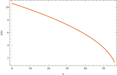
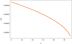
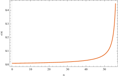
Figure 1: Plots of $\psi(n)$ — on the left — $\chi(n)$ — in the center — and $\epsilon(n)$ — on the right — for $0\leq n\leq 56$.

Figure 2 shows the same three quantities through the end of inflation (which occurs at $n_{e}\simeq 56.7$) under the assumption that the classical relations (36-38) are not corrected by the quantum effects we seek to incorporate. During this phase the inflaton oscillates around $\psi=0$ with decreasing amplitude and increasing frequency, while the first slow roll parameter oscillates in the range $0\leq\epsilon\leq 3$. Because $\epsilon={\psi^{\prime}}^{2}$, the first slow roll parameter vanishes at extrema of $\psi(n)$, and it reaches its maximum (of $\epsilon(n)=3$) when $\psi(n)=0$. Of course the dimensionless Hubble parameter is monotonically decreasing; this decrease is rapid when $\epsilon\simeq 3$, and slow when $\epsilon\simeq 0$.

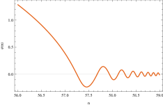
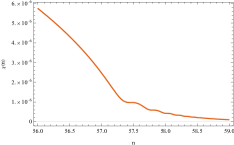
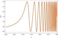
Figure 2: Plots of $\psi(n)$ — on the left — $\chi(n)$ — in the center — and $\epsilon(n)$ — on the right — for $56\leq n\leq 59$.

The slow roll approximation (46) tells us that $\psi^{\prime}\simeq-1/\psi$ and $\chi(n)\simeq c/\sqrt{3}\times\psi(n)$. Setting $D=4$, and using our values of $c=7.1\times 10^{-6}$ and $q=1.2\times 10^{-6}$, gives the mass hierarchy,

$$\frac{\mu^{2}_{u}}{\chi^{2}}\simeq 2+\frac{6q^{2}}{c^{2}}\simeq 2.16\quad>\quad\frac{\mu^{2}}{\chi^{2}}\simeq\frac{6q^{2}}{c^{2}}\simeq 0.16\quad>\quad\frac{\mu^{2}_{t}}{\chi^{2}}\simeq\frac{3}{\psi^{2}}\;.$$ (48)

Figure 3 shows the various masses through inflation.

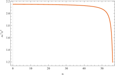
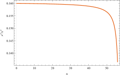
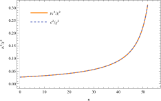
Figure 3: Plots of $\mu_{u}^{2}(n)/\chi^{2}(n)$ — on the left — $\mu^{2}(n)/\chi^{2}(n)$ — in the center — and $\mu^{2}_{t}(n)/\chi^{2}(n)$ — on the right — for $0\leq n\leq 56$.

As one can just see from the larger $n$ values of Figure 3, the hierarchy of equation (48) becomes inverted after the end of inflation. Figure 4 shows the behavior after the end of inflation. During this phase $\mu^{2}_{u}/\chi^{2}$ is mostly tachyonic, and actually diverges at points where $\psi(n)=0$. On the other hand, $\mu^{2}/\chi^{2}$ oscillates between $0$ and the small value of $0.16$, while $\mu^{2}_{t}/\chi^{2}$ grows monotonically to large, positive values. The $u$-mode mass is the most important of the three, and its evolution is the most complex. Figure 5 shows its behavior in more detail.

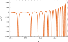
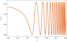
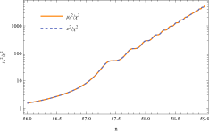
Figure 4: Plots of $\mu_{u}^{2}(n)/\chi^{2}(n)$ — on the left — $\mu^{2}(n)/\chi^{2}(n)$ — in the center — and $\mu^{2}_{t}(n)/\chi^{2}(n)$ — on the right — for $56\leq n\leq 59$.

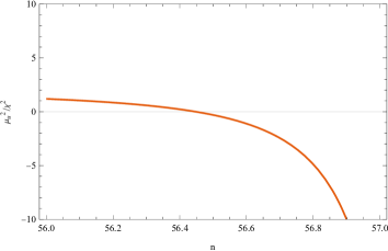
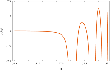
Figure 5: The left hand plot shows $\mu_{u}^{2}(n)/\chi^{2}(n)$ on the range $56\leq n\leq 57$, just before the first zero of $\mu(n)$. The right hand plot depicts $\mu_{u}^{2}(n)/\chi^{2}(n)$ over the slightly larger range of $56\leq n\leq 58$, which includes the first three zeroes of $\mu(n)$.

3.2 Approximating the Longitudinal Amplitude

Equation (41) for $\mathcal{T}(n,\kappa)$ contains six terms. The ultraviolet regime is defined by the condition $\kappa\gg\chi(n)e^{n}$. In this regime equation (41) is dominated by the 4th and 6th terms, $2\kappa^{2}e^{-2n}/\chi^{2}$ and $-e^{-2[\mathcal{T}+(D-1)n]}/2\chi^{2}$, and the amplitude takes the form,

$$\mathcal{T}(n,\kappa)=\ln\Bigl{[}\frac{1}{2\kappa}\Bigr{]}-(D\!-\!2)n$$ (49)

$$\hskip 76.82234pt+\Bigl{[}\frac{1}{2}(D\!-\!2)(D\!-\!2\epsilon)-\frac{2\mu_{t}^{2}}{\chi^{2}}\Bigr{]}\Bigl{(}\frac{\chi e^{n}}{2\kappa}\Bigr{)}^{2}+O\Biggl{(}\Bigl{(}\frac{\chi e^{n}}{2\kappa}\Bigr{)}^{4}\Biggr{)}\;.\qquad$$

Figure 6 compares numerical evolution of the exact equation (41) with the ultraviolet form (49) for wave numbers which experience first horizon crossing at $n_{1}=10$, $n_{1}=20$, and $n_{1}=30$. The agreement is excellent up to horizon crossing.

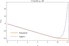
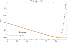
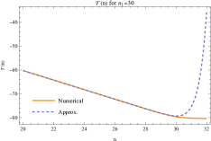
Figure 6: Plot comparing $\mathcal{T}(n,\kappa)$ with the ultraviolet form (49) for modes which experience first horizon crossing at $n_{1}=10$ (left), $n_{1}=20$ (center) and $n_{1}=30$ (right).

After 1st horizon crossing the 4th and 6th terms of (41) effectively drop out and the relation simplifies to,

$$\mathcal{T}^{\prime\prime}+\frac{1}{2}{\mathcal{T}^{\prime}}^{2}+(D\!-\!1\!-\!\epsilon)\mathcal{T}^{\prime}-2(D\!-\!1\!-\!\epsilon)\frac{\mu^{\prime}}{\mu}-2\frac{\mu^{\prime\prime}}{\mu}\simeq 0\;.$$ (50)

This is an equation for $\mathcal{T}^{\prime}$, and it is easy to see that a particular solution is,

$$\mathcal{T}^{\prime}=2\frac{\mu^{\prime}}{\mu}\;.$$ (51)

Integrating (51), and using the tensor power spectrum to infer the integration constant to all orders in the slow roll approximation [7], implies,

$$\mathcal{T}(n,\kappa)\simeq\ln\Biggl{[}\frac{\chi_{1}^{2}C(\epsilon_{1})}{2\kappa^{3}}\times\frac{\mu^{2}(n)}{\mu^{2}_{1}}\Biggr{]}\;,$$ (52)

where the function $C(\epsilon)$ is,

$$C(\epsilon)=\frac{1}{\pi}\Gamma^{2}\Bigl{(}\frac{1}{2}\!+\!\frac{1}{1\!-\!\epsilon}\Bigr{)}\Bigl{[}2(1\!-\!\epsilon)\Bigr{]}^{\frac{2}{1-\epsilon}}\;.$$ (53)

Figure 7 compares the exact numerical result with the infrared form (52) for modes which experience horizon crossing at $n_{1}=10$, $n_{1}=20$, and $n_{1}=30$. Agreement is excellent.

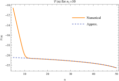
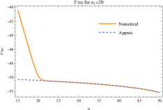
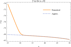
Figure 7: Plot comparing $\mathcal{T}(n,\kappa)$ with the late time form (52) for modes which experience first horizon crossing at $n_{1}=10$ (left), $n_{1}=20$ (center) and $n_{1}=30$ (right).

Although one can see from Figure 7 that the approximate solution (52) is highly accurate, it cannot be exact for two reasons:

1. We neglected the 4th and 6th terms in simplifying equation (41) to reach (50); and

2. Just because (51) is a solution to (50) does not mean it is the solution.

To find the general solution to (50) we substitute $\mathcal{T}^{\prime}=2\mu^{\prime}/\mu+f(n)$,

$$f^{\prime}+2\frac{\mu^{\prime}}{\mu}f+\frac{1}{2}f^{2}+(D\!-\!1\!-\!\epsilon)f\simeq 0\;.$$ (54)

Now divide by $\mu^{2}e^{(D-1)n}\chi f^{2}$ to reach the form,

$$\frac{\partial}{\partial n}\Biggl{[}\frac{1}{\mu^{2}e^{(D-1)n}\chi f}\Biggr{]}=\frac{1}{2\mu^{2}e^{(D-1)n}\chi}\;.$$ (55)

Integrating equation (55) from some point $n_{2}$ gives the general solution,

$$f(n)=f_{2}\Biggl{[}e^{(D-1)(n-n_{2})}\Bigl{[}\frac{\chi(n)}{\chi_{2}}\Bigr{]}\Bigl{[}\frac{\mu(n)}{\mu_{2}}\Bigr{]}^{2}$$ (56)

$$\hskip 113.81102pt+\frac{1}{2}f_{2}\int_{n_{2}}^{n}\!\!\!\!\!dn^{\prime}\,e^{(D-1)(n-n^{\prime})}\Bigl{[}\frac{\chi(n)}{\chi(n^{\prime})}\Bigr{]}\Bigl{[}\frac{\mu(n)}{\mu(n^{\prime})}\Bigr{]}^{2}\Biggr{]}^{-1}\;.\qquad$$

Careful consideration of (56) reveals that $\mathcal{T}(n,\kappa)$ actually has a finite limit as the mass vanishes. To see this, assume $n$ is such that $\mu(n)\rightarrow 0$, and expand the integral of (56) for small $\mu(n)$,

$$\int_{n_{2}}^{n}\!\!\!\!\!dn^{\prime}\,e^{(D-1)(n-n^{\prime})}\Bigl{[}\frac{\chi(n)}{\chi(n^{\prime})}\Bigr{]}\Bigl{[}\frac{\mu(n)}{\mu(n^{\prime})}\Bigr{]}^{2}\!\!=-\frac{\mu(n)}{\mu^{\prime}(n)}$$ (57)

$$\hskip 56.9055pt-\frac{1}{2}\Bigl{[}D\!-\!1\!-\!\epsilon(n)\!+\!\frac{\mu^{\prime\prime}(n)}{\mu^{\prime}(n)}\Bigr{]}\Bigl{[}\frac{\mu(n)}{\mu^{\prime}(n)}\Bigr{]}^{2}\ln[\mu^{2}(n)]+O(1)\;.\qquad$$

Near the point where $\mu(n)\rightarrow 0$ we therefore have,

$$f(n)\longrightarrow-\frac{2\mu^{\prime}(n)}{\mu(n)}+\Bigl{[}D\!-\!1\!-\!\epsilon(n)\!+\!\frac{\mu^{\prime\prime}(n)}{\mu^{\prime}(n)}\Bigr{]}\ln[\mu^{2}(n)]+O(1)\;.$$ (58)

Hence we have,

$$\mathcal{T}^{\prime}(n,\kappa)\longrightarrow\Bigl{[}D\!-\!1\!-\!\epsilon(n)\!+\!\frac{\mu^{\prime\prime}(n)}{\mu^{\prime}(n)}\Bigr{]}\ln[\mu^{2}(n)]+O(1)\;.$$ (59)

Although expression (59) diverges as $\mu(n)$ goes to zero, the singularity is integrable, which means that $\mathcal{T}(n,\kappa)$ remains finite.

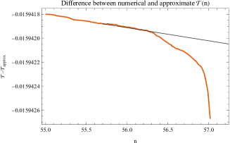
Figure 8: Numerical determination of the constant $f_{2}$ from the difference of $\mathcal{T}(n,\kappa)$ and expression (52). In this case $\kappa$ was chosen to experience first horizon crossing at $n_{1}=10$.

As we see from Figure 8, the constant $f_{2}$ in expression (56) represents the difference between the actual value of $\mathcal{T}^{\prime}(n_{2},\kappa)$ and its approximate form (51) $2\mu^{\prime}(n_{2})/\mu(n_{2})$. Because the approximate form is quite accurate, $f_{2}$ is a very small number, about $f_{2}\sim-10^{-7}$. The fact that $f_{2}$ drops out of the asymptotic form (58) means that the ultimate finiteness of $\mathcal{T}(n,\kappa)$ is a robust conclusion. However, $\mu(n)$ must be very close to zero before the integral (57) begins to dominate over the first term in the denominator of (56), which has a relative enhancement of $e^{(D-1)(n-n_{2})}$. If we take $n_{2}=56$ and define $n_{*}\simeq 57.25$ as the first zero of $\mu(n)$, the point $n_{f}$ at which expressions (58-59) become valid approximately obeys,

$$n_{*}-n_{f}\simeq\frac{1}{2}f_{2}\,e^{-3(n_{*}-n_{2})}\Bigl{(}\frac{\chi_{2}}{\chi_{*}}\Bigr{)}\Bigl{(}\frac{\mu_{2}}{\mu_{*}^{\prime}}\Bigr{)}^{2}\simeq 10^{-9}\;.$$ (60)

We can therefore estimate the minimum value of $\mathcal{T}(n,\kappa)$ as

$$\mathcal{T}_{\rm min}\simeq\ln\Biggl{[}\frac{\chi_{1}^{2}C(\epsilon_{1})}{2\kappa^{3}}\!\times\!\frac{1}{4}f_{2}^{2}\,e^{-6(n_{*}-n_{2})}\Bigl{(}\frac{\chi_{2}}{\chi_{*}}\Bigr{)}^{2}\Bigl{(}\frac{\mu_{2}}{\mu_{1}}\Bigr{)}^{2}\Bigl{(}\frac{\mu_{2}}{\mu_{*}^{\prime}}\Big{)}^{2}\Biggr{]}\;.$$ (61)

3.3 Approximating the Temporal Amplitude

Equation (42) for $\mathcal{U}(n,\kappa)$ contains the same six terms as (41). In the ultraviolet it is also dominated by the 4th and 6th terms, $2\kappa^{2}e^{-2n}/\chi^{2}$ and $-e^{-2[\mathcal{U}+(D-1)n]}/2\chi^{2}$. Hence the ultraviolet expansion of $\mathcal{U}(n,\kappa)$ takes the same form as (49),

$$\mathcal{U}(n,\kappa)=\ln\Bigl{[}\frac{1}{2\kappa}\Bigr{]}-(D\!-\!2)n$$ (62)

$$\hskip 76.82234pt+\Bigl{[}\frac{1}{2}(D\!-\!2)(D\!-\!2\epsilon)-\frac{2\mu_{u}^{2}}{\chi^{2}}\Bigr{]}\Bigl{(}\frac{\chi e^{n}}{2\kappa}\Bigr{)}^{2}+O\Biggl{(}\Bigl{(}\frac{\chi e^{n}}{2\kappa}\Bigr{)}^{4}\Biggr{)}\;.\qquad$$

Figure 9 compares the exact numerical solution with the ultraviolet form (62) for modes which experience first horizon crossing at $n_{1}=10$, $n_{1}=20$ and $n_{1}=30$. Agreement is excellent up to first horizon crossing, just as it was in the analogous comparison of Figure 6 for $\mathcal{T}(n,\kappa)$.

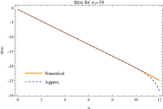
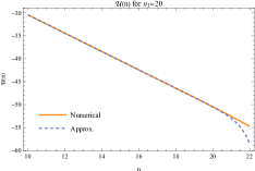
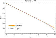
Figure 9: Plot comparing $\mathcal{U}(n,\kappa)$ with the ultraviolet form (62) for modes which experience first horizon crossing at $n_{1}=10$ (left), $n_{1}=20$ (center) and $n_{1}=30$ (right).

The 4th and 6th terms of (42) drop out after first horizon crossing, and the relation simplifies to,

$$\mathcal{U}^{\prime\prime}+\frac{1}{2}{\mathcal{U}^{\prime}}^{2}+(D\!-\!1\!-\!\epsilon)\mathcal{U}^{\prime}+\frac{2\mu^{2}_{u}}{\chi^{2}}\simeq 0\;.$$ (63)

Recall from Figure 3 that $\mu_{u}^{2}(n)/\chi^{2}(n)$ is approximately constant during inflation. This means that equation (63) can be roughly solved as,

$$\mathcal{U}^{\prime}(n,\kappa)\simeq-(D\!-\!1\!-\!\epsilon)+\sqrt{(D\!-\!1\!-\!\epsilon)^{2}-\frac{4\mu_{u}^{2}}{\chi^{2}}}\;.$$ (64)

With the appropriate integration constant we therefore have,

$$\mathcal{U}(n,\kappa)\simeq\ln\Biggl{[}\frac{\chi_{1}^{2}C(\epsilon_{1})}{2\kappa^{3}}\!\times\!\frac{\chi_{1}}{\chi(n)}\Biggl{]}-(D\!-\!1)(n\!-\!n_{1})$$ (65)

$$\hskip 142.26378pt+\int_{n_{1}}^{n}\!\!\!\!dn^{\prime}\sqrt{[D\!-\!1\!-\!\epsilon(n^{\prime})]^{2}-\frac{4\mu_{u}^{2}(n^{\prime})}{\chi^{2}(n^{\prime})}}\;.\qquad$$

Figure 10 compares this approximation with the numerical evolution for modes which experience horizon crossing at $n_{1}=10$, $n_{1}=20$ and $n_{1}=30$.

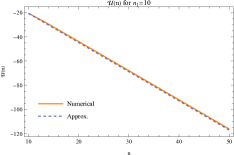
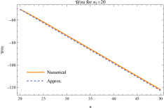
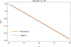
Figure 10: Plot comparing $\mathcal{U}(n,\kappa)$ with the late time form (65) for modes which experience first horizon crossing at $n_{1}=10$ (left), $n_{1}=20$ (center) and $n_{1}=30$ (right).

After the end of inflation $\mu^{2}(n)/\chi^{2}(n)$ falls off whereas the derivative terms in $\mu^{2}_{u}/\chi^{2}$ become large and tachyonic. This means we can neglect $\mu^{2}(n)/\chi^{2}(n)$,

$$\frac{\mu_{u}^{2}}{\chi^{2}}\simeq(D\!-\!2)(1\!-\!\epsilon)-(D\!-\!3\!+\!\epsilon)\frac{\mu^{\prime}}{\mu}+\Bigl{(}\frac{\mu^{\prime}}{\mu}\Bigr{)}^{\prime}-\Bigl{(}\frac{\mu^{\prime}}{\mu}\Bigr{)}^{2}\;.$$ (66)

We now make the substitution,

$$\mathcal{U}^{\prime}(n,\kappa)=-\frac{2\mu^{\prime}(n)}{\mu(n)}-2(D\!-\!2)+g(n)\;,$$ (67)

in equation (63) to find,

$$g^{\prime}-\Bigl{(}D\!-\!3\!+\!\epsilon\!+\!2\frac{\mu^{\prime}}{\mu}\Bigr{)}g+\frac{1}{2}g^{2}=0\;.$$ (68)

Multiplying by $e^{(D-3)n}\mu^{2}(n)/[\chi(n)g^{2}(n)]$ makes the $g$-dependent terms a total derivative, and permits us to write the general solution as,

$$g(n)=g_{2}\Biggl{[}e^{-(D-3)(n-n_{2})}\Bigl{[}\frac{\chi(n)}{\chi_{2}}\Bigr{]}\Bigl{[}\frac{\mu_{2}}{\mu(n)}\Bigr{]}^{2}$$ (69)

$$\hskip 113.81102pt+\frac{1}{2}g_{2}\!\!\int_{n_{2}}^{n}\!\!\!\!\!dn^{\prime}\,e^{-(D-3)(n-n^{\prime})}\Bigl{[}\frac{\chi(n)}{\chi(n^{\prime})}\Bigr{]}\Bigl{[}\frac{\mu(n^{\prime})}{\mu(n)}\Bigr{]}^{2}\Biggr{]}^{-1}\;,\qquad$$

where the constant $g_{2}$ is determined to interpolate between (64) and (67),

$$g_{2}=\frac{2\mu_{2}^{\prime}}{\mu_{2}}+(D\!-\!3\!+\!\epsilon_{2})+\sqrt{(D\!-\!1\!-\!\epsilon_{2})^{2}-\frac{4\mu_{2}^{2}}{\chi_{2}^{2}}}\;.$$ (70)

Note that, whereas $f(n)$ diverges as $\mu(n)$ approaches zero, $g(n)$ goes to zero like $\mu^{2}(n)$.

Integrating equation (67), and using (65) to supply the integration constant, gives,

$$\mathcal{U}(n,\kappa)\simeq\ln\Biggl{[}\frac{\chi_{1}^{2}C(\epsilon_{1})}{2\kappa^{3}}\!\times\!\frac{\chi_{1}}{\chi_{2}}\!\times\!\frac{\mu_{2}^{2}}{\mu^{2}(n)}\Biggr{]}-(D\!-\!1)(n_{2}\!-\!n_{1})-2(D\!-\!2)(n\!-\!n_{2})$$ (71)

$$\hskip 91.04872pt+\int_{n_{1}}^{n_{2}}\!\!\!\!\!dn^{\prime}\sqrt{[D\!-\!1\!-\!\epsilon(n^{\prime})]^{2}-\frac{4\mu_{u}^{2}(n^{\prime})}{\chi^{2}(n^{\prime})}}+\int_{n_{2}}^{n}\!\!\!\!\!dn^{\prime}\,g(n^{\prime})\;.\qquad$$

Because $g(n)$ vanishes as $\mu(n)\rightarrow 0$, the $-\ln[\mu^{2}(n)]$ divergence of $\mathcal{U}(n,\kappa)$ is robust. Note that this is not even affected by neglecting $\mu^{2}(n)/\chi^{2}(n)$ in (66). Figure 11 compares the numerical solution with our analytic approximation (71).

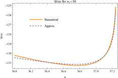
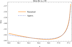
Figure 11: Plot comparing $\mathcal{U}(n,\kappa)$ with the post-inflationary form (71) for modes which experience first horizon crossing at $n_{1}=10$ (left), $n_{1}=20$ (center) and $n_{1}=30$ (right).

4 Quantum-Correcting the Inflaton $0$-Mode

The purpose of this section is to use the photon propagator to quantum-correct the classical equation for the inflaton $0$-mode from (15) to,

$$\partial_{0}\Bigl{[}a^{D-2}\partial_{0}\varphi_{0}\Bigr{]}+a^{D}\varphi_{0}V^{\prime}(\varphi_{0}^{2})+q^{2}\varphi_{0}a^{D-2}\eta^{\mu\nu}i\Bigl{[}\mbox{}_{\mu}\Delta_{\nu}\Bigr{]}(x;x)=0\;.$$ (72)

We begin by deriving exact expressions for the $t$-mode and $u$-mode contributions to the trace of the photon propagator. We then use a variant of the work-energy theorem to show how reheating occurs.

4.1 The Effective Force

The $t$-mode contribution to the coincidence limit of the trace of the photon propagator in equation (72) is,

$$\sqrt{-g}\,g^{\mu\nu}i\Bigl{[}\mbox{}_{\mu}\Delta_{\nu}\Bigr{]}_{t}(x;x)=a^{D-2}\!\!\int\!\!\frac{d^{D-1}k}{(2\pi)^{D-1}}\Biggl{\{}\frac{1}{M^{2}}\,\widehat{\partial}_{0}t\!\cdot\!\widehat{\partial_{0}}t^{*}-\frac{k^{2}}{M^{2}}\,t\!\cdot\!t^{*}\Biggr{\}}\;.$$ (73)

The $t$-mode equation (27) can be exploited to write the product of time derivatives in terms of the norm-squared,

$$\partial_{0}t\!\cdot\!\partial_{0}t^{*}=\Bigl{[}\frac{1}{2}\partial_{0}^{2}+\frac{1}{2}(D\!-\!2)aH\partial_{0}+k^{2}-(D\!-\!2)aH\frac{\partial_{0}M}{M}-\frac{\partial_{0}^{2}M}{M}\Bigr{]}(tt^{*})\;.$$ (74)

Using this identity we can re-express the $t$-mode contribution (73) as,

$$\sqrt{-g}\,g^{\mu\nu}i\Bigl{[}\mbox{}_{\mu}\Delta_{\nu}\Bigr{]}_{t}=\frac{a^{D-2}}{M^{2}}\!\!\int\!\!\frac{d^{D-1}k}{(2\pi)^{D-1}}\Biggl{\{}\frac{1}{2}\partial_{0}^{2}+\frac{1}{2}(D\!-\!2)aH\partial_{0}-\frac{\partial_{0}M}{M}\partial_{0}$$ (75)

$$\hskip 113.81102pt-(D\!-\!2)aH\frac{\partial_{0}M}{M}-\frac{\partial_{0}^{2}M}{M}+\Bigl{(}\frac{\partial_{0}M}{M}\Bigr{)}^{2}\Biggr{\}}(tt^{*})\;.\qquad$$

Converting to dimensionless form, and employing equation (41) to eliminate second derivatives, gives the compact form,

$$\sqrt{-g}\,g^{\mu\nu}i\Bigl{[}\mbox{}_{\mu}\Delta_{\nu}\Bigr{]}_{t}(x;x)=\frac{e^{Dn}\chi^{2}(n)}{(8\pi G)^{\frac{D}{2}-1}\mu^{2}(n)}\!\!\int\!\!\frac{d^{D-1}\kappa}{(2\pi)^{D-1}}\,e^{\mathcal{T}(n,\kappa)}$$ (76)

$$\hskip 36.98866pt\times\Biggl{\{}\Bigl{[}\frac{1}{2}\mathcal{T}^{\prime}(n,\kappa)-\frac{\mu^{\prime}(n)}{\mu(n)}\Bigr{]}^{2}-\frac{\kappa^{2}e^{-2n}}{\chi^{2}(n)}+\frac{1}{4\chi^{2}}e^{-2[\mathcal{T}(n,\kappa)+(D-1)n]}\Biggr{\}}.\qquad$$

The $u$-mode contribution to the photon trace in (72) is,

$$\sqrt{-g}\,g^{\mu\nu}i\Bigl{[}\mbox{}_{\mu}\Delta_{\nu}\Bigr{]}_{u}(x;x)=a^{D-2}\!\!\int\!\!\frac{d^{D-1}k}{(2\pi)^{D-1}}\Biggl{\{}-\frac{k^{2}}{M^{2}}\,u\!\cdot\!u^{*}+\frac{1}{M^{2}}\widetilde{D}u\!\cdot\!\widetilde{D}u^{*}\Biggr{\}}\;.$$ (77)

We can eliminate the norm-square of $\partial_{0}u$ using the $u$-mode equation (29),

$$\partial_{0}u\!\cdot\!\partial_{0}u^{*}=\Biggl{[}\frac{1}{2}\partial_{0}^{2}+\frac{1}{2}(D\!-\!2)aH\partial_{0}+k^{2}+a^{2}M^{2}+(D\!-\!2)a^{2}H^{2}(1\!-\!\epsilon)$$ (78)

$$\hskip 91.04872pt-(D\!-\!2)aH\frac{\partial_{0}M}{M}+\partial_{0}\Bigl{(}\frac{\partial_{0}M}{M}\Bigr{)}-\Bigl{(}\frac{\partial_{0}M}{M}\Bigr{)}^{2}\Biggr{]}(uu^{*})\;.\qquad$$

Substituting (78) in (77), and taking apart the factors of $\widetilde{D}=\partial_{0}+(D-2)aH+\partial_{0}M/M$ gives,

$$\sqrt{-g}\,g^{\mu\nu}i\Bigl{[}\mbox{}_{\mu}\Delta_{\nu}\Bigr{]}_{u}=\frac{a^{D-2}}{M^{2}}\!\!\int\!\!\frac{d^{D-1}k}{(2\pi)^{D-1}}\Biggl{\{}\frac{1}{2}\partial_{0}^{2}+\frac{3}{2}(D\!-\!2)aH\partial_{0}+\frac{\partial_{0}M}{M}\partial_{0}+a^{2}M^{2}$$ (79)

$$\hskip 19.91684pt+(D\!-\!2)(D\!-\!1\!-\!\epsilon)a^{2}H^{2}+(D\!-\!2)aH\frac{\partial_{0}M}{M}+\partial_{0}\Bigl{(}\frac{\partial_{0}M}{M}\Bigr{)}\Biggr{\}}(uu^{*})\;.\qquad$$

The final, dimensionless form is very similar to (76),

$$\sqrt{-g}\,g^{\mu\nu}i\Bigl{[}\mbox{}_{\mu}\Delta_{\nu}\Bigr{]}_{u}(x;x)=\frac{e^{Dn}\chi^{2}(n)}{(8\pi G)^{\frac{D}{2}-1}\mu^{2}(n)}\!\!\int\!\!\frac{d^{D-1}\kappa}{(2\pi)^{D-1}}\,e^{\mathcal{U}(n,\kappa)}$$ (80)

$$\times\Biggl{\{}\Bigl{[}\frac{1}{2}\mathcal{U}^{\prime}(n,\kappa)+\frac{\mu^{\prime}(n)}{\mu(n)}+D\!-\!2\Bigr{]}^{2}-\frac{\kappa^{2}e^{-2n}}{\chi^{2}(n)}+\frac{1}{4\chi^{2}}e^{-2[\mathcal{U}(n,\kappa)+(D-1)n]}\Biggr{\}}.\qquad$$

4.2 Reheating

The dimensionless form of the inflaton $0$-mode equation (72) takes the form,

$$e^{n}\chi\frac{\partial}{\partial n}\Bigl{[}e^{(D-1)n}\chi\psi^{\prime}\Bigr{]}=-e^{Dn}\psi\Biggl{[}U^{\prime}(\psi^{2})+\frac{Q^{2}\chi^{2}}{\mu^{2}}\!\!\int\!\!\frac{d^{D-1}\kappa}{(2\pi)^{D-1}}\Biggl{\{}\qquad\Biggr{\}}\Biggr{]}\equiv\mathcal{F}\;.$$ (81)

where the term inside the curly brackets is the sum of the $t$ and $u$ contributions from expressions (76) and (80), and $Q^{2}\equiv q^{2}/(8\pi G)^{\frac{D}{2}-2}$ is the dimensionless charge. Multiplying both sides of (81) by $e^{(D-2)n}\chi\psi^{\prime}$ and integrating gives a curious generalization of the famous work-energy theorem of introductory physics,

$$e^{(D-1)n}\chi\psi^{\prime}\frac{\partial}{\partial n}\Bigl{[}e^{(D-1)n}\chi\psi^{\prime}\Bigr{]}=\frac{1}{2}\frac{\partial}{\partial n}\Bigl{[}e^{(D-1)n}\chi\psi^{\prime}\Bigr{]}^{2}=e^{(D-2)n}\chi\psi^{\prime}\!\times\!\mathcal{F}\;.$$ (82)

We now integrate (82) from the beginning of reheating (at $n=n_{i}$) to the end (at $n=n_{f}$), and use the fact that $\psi^{\prime}(n_{f})=0$ at the end of reheating,

$$0-\frac{1}{2}\Bigl{[}e^{(D-1)n_{i}}\chi_{i}\psi^{\prime}_{i}\Bigr{]}^{2}=\int_{n_{i}}^{n_{f}}\!\!\!\!dn\,e^{(D-2)n}\chi(n)\psi^{\prime}(n)\mathcal{F}(n)\;.$$ (83)

Equation (83) clearly implies that the product of $\psi^{\prime}(n)\times\mathcal{F}(n)$ must be negative in order to suck the energy out of the inflaton $0$-mode. The classical contribution from $\psi^{\prime}\times-\psi U^{\prime}(\psi^{2})$ is positive, so reheating must be driven by the quantum corrections from the $t$-modes and the $u$-modes, each of which has two positive and one negative contribution. From expressions (76) and (80) we see that the desired negative contribution can only come from the $-\kappa^{2}e^{-2n}/\chi^{2}(n)$ terms, however, it is not clear if the dominant effect comes from $t$-modes or $u$-modes. It is also not clear whether the largest contributions come from super-horizon modes (with $\kappa<\chi(n_{e})e^{n_{e}}$, where $n_{e}$ denotes the end of inflation) or sub-horizon modes (with $\kappa>\chi(n_{e})e^{n_{e}}$). Note that discretization can only recover the longest wavelength sub-horizon modes.

Let us first examine sub-horizon modes, for which $\chi e^{n}/\kappa$ is small. In this case the ultraviolet expansions (49) and (62) imply that the multiplicative exponentials agree to leading order,

$$e^{\mathcal{T}(n,\kappa)}=\frac{e^{-(D-2)n}}{2\kappa}\Biggl{\{}1+O\Bigl{(}\frac{\chi^{2}e^{2n}}{\kappa^{2}}\Bigr{)}\Biggr{\}}\;\;,\;\;e^{\mathcal{U}(n,\kappa)}=\frac{e^{-(D-2)n}}{2\kappa}\Biggl{\{}1+O\Bigl{(}\frac{\chi^{2}e^{2n}}{\kappa^{2}}\Bigr{)}\Biggr{\}}\;.$$ (84)

Substituting the same ultraviolet expansions into the curly bracketed parts of (76) and (80) gives,

$$\Bigl{[}\frac{1}{2}\mathcal{T}^{\prime}-\frac{\mu^{\prime}}{\mu}\Bigr{]}^{2}-\frac{\kappa^{2}e^{-2n}}{\chi^{2}}+\frac{e^{-2[\mathcal{T}+(D-1)n]}}{4\chi^{2}}$$ (85)

$$\hskip 56.9055pt=-\frac{1}{2}(D\!-\!2)(1\!-\!\epsilon)-(1\!-\!\epsilon)\frac{\mu^{\prime}}{\mu}-\Bigl{(}\frac{\mu^{\prime}}{\mu}\Bigr{)}^{\prime}+O\Bigl{(}\frac{\chi^{2}e^{2n}}{\kappa^{2}}\Bigr{)}\;,\qquad$$

$$\Bigl{[}\frac{1}{2}\mathcal{U}^{\prime}+\frac{\mu^{\prime}}{\mu}+D\!-\!2\Bigr{]}^{2}-\frac{\kappa^{2}e^{-2n}}{\chi^{2}}+\frac{e^{-2[\mathcal{U}+(D-1)n]}}{4\chi^{2}}$$ (86)

$$\hskip 56.9055pt=\frac{1}{2}(D\!-\!2)(1\!-\!\epsilon)+(1\!-\!\epsilon)\frac{\mu^{\prime}}{\mu}+\Bigl{(}\frac{\mu^{\prime}}{\mu}\Bigr{)}^{\prime}+O\Bigl{(}\frac{\chi^{2}e^{2n}}{\kappa^{2}}\Bigr{)}\;.\qquad$$

Hence there is perfect cancellation between the sub-horizon $t$-mode and $u$-mode contributions at leading order.

Super-horizon modes cannot show the same cancellation because $\mathcal{T}(n,\kappa)$ approaches a large, negative constant (61) as $\mu(n)$ goes to zero, whereas $\mathcal{U}(n,\kappa)$ diverges like $\mathcal{U}_{*}+\ln[\mu_{2}^{2}/\mu^{2}(n)]$. This means that the multiplicative exponentials take the form,

$$e^{\mathcal{T}(n,\kappa)}\longrightarrow e^{\mathcal{T}_{\rm min}}\qquad,\qquad e^{\mathcal{U}(n,\kappa)}\longrightarrow e^{\mathcal{U}_{*}}\Bigl{[}\frac{\mu_{2}}{\mu(n)}\Bigr{]}^{2}\;.$$ (87)

The curly bracketed terms which involve explicit factors of $\mu^{\prime}/\mu$ wind up depending on the functions $f(n)$ and $g(n)$, given in expressions (56) and (69), respectively,

$$\Bigl{[}\frac{1}{2}\mathcal{T}^{\prime}-\frac{\mu^{\prime}}{\mu}\Bigr{]}^{2} \!\!\!=\!\!\! \frac{1}{4}f^{2}(n)\longrightarrow\Bigl{[}\frac{\mu^{\prime}(n)}{\mu(n)}\Bigr{]}^{2}\;,$$ (88)

$$\Bigl{[}\frac{1}{2}\mathcal{U}^{\prime}+\frac{\mu^{\prime}}{\mu}+D\!-\!2\Bigr{]}^{2} \!\!\!=\!\!\! \frac{1}{4}g^{2}(n)\longrightarrow 0\;.$$ (89)

This means that the $t$-modes contribute positively, while the $u$-modes make a negative contribution,

$$e^{\mathcal{T}}\!\times\!\Biggl{\{}\qquad\Biggr{\}} \!\!\!\longrightarrow\!\!\! e^{\mathcal{T}_{\rm min}}\Bigl{[}\frac{\mu^{\prime}(n)}{\mu(n)}\Bigr{]}^{2}\;,$$ (90)

$$e^{\mathcal{U}}\!\times\!\Biggl{\{}\qquad\Biggr{\}} \!\!\!\longrightarrow\!\!\! e^{\mathcal{U}_{*}}\Bigl{[}\frac{\mu_{2}}{\mu(n)}\Bigr{]}^{2}\!\times\!-\frac{\kappa^{2}e^{-2n_{*}}}{\chi_{*}^{2}}\;.\qquad$$ (91)

How large the relative coefficients are depends on the integration constant $f_{2}$, for which we do not yet have an analytic form.

Whether (90) or (91) dominates, it is significant that both terms diverge like $1/\mu^{2}(n)$. Because the effective force contains another factor of $1/\mu^{2}(n)$, this means that the quantum correction diverges like $1/\mu^{4}(n)$ near the point $n_{*}$ at which $\mu(n)$ vanishes. The measure factor in (83) softens this somewhat, but not enough,

$$Q^{2}\psi^{\prime}(n)\psi(n)dn=\frac{1}{4}d\mu^{2}\;.$$ (92)

The integral (83) therefore diverges before $\mu(n)=0$, which presumably brings reheating to an end.

5 Conclusions

Ema et al. have shown that coupling a charged inflaton to electromagnetism provides the most efficient reheating [1]. The mechanism is that the inflaton’s evolution induces a time-dependent photon mass through the Higgs mechanism. Nothing special changes about the transverse spatial polarizations, but inverse powers of the mass appear in the longitudinal-temporal polarizations (26) and (28), which result from the photon having “eaten” the phase of the inflaton field. These factors diverge when the inflaton passes through zero. The effect is strengthened by factors of $\mu^{\prime}(n)/\mu(n)$ which appear in the mass terms (43-44) of the two modes.

Our paper represents an effort to improve on previous excellent numerical studies of this process based on discretizing space [2]. Although that method can accommodate arbitrarily strong photon fields, it is of course limited to a finite range of sub-horizon modes. In contrast, we use the trace of the coincident photon propagator to study the inflaton $0$-mode equation (72). Our expressions (75-76) and (79-80) for the longitudinal and temporal contributions to this trace are exact. They can be used to include the effects of super-horizon modes, and of arbitrarily short wave length modes. In fact, our use of dimensional regularization means that the far ultraviolet can be included as well, through the use of expansions (49) and (62).

We have also derived good analytic approximations for the amplitudes. Before first horizon crossing these are (49) and (62), respectively. After first crossing the $t$-mode amplitude is well approximated by expression (52) until close to the point at which $\mu(n)=0$. However, expression (59) shows that the $t$-mode amplitude remains finite when $\mu(n)=0$.

Two forms are required to approximate the $u$-mode amplitude after first horizon crossing, owing to its dependence on the complicated behavior of the $u$-mode mass term (44), which is evident from Figures 4 and 5. During inflation, the near constancy of $\epsilon(n)$ and $\mu^{2}_{u}(n)/\chi^{2}(n)$, result in expression (65) giving a good approximation. After the end of inflation the better approximation is provided by expression (71). Because this last form becomes exact as $\mu(n)\rightarrow 0$, we know that the $u$-mode amplitude diverges like $-\ln[\mu^{2}(n)]$, which provides an extra factor of $1/\mu^{2}(n)$ in the trace of the photon propagator (80).

The obvious next step is to exploit the powerful analytic expressions we have derived to make a detailed numerical study of reheating in a realistic model, such as Starobinsky inflation [12], Higgs inflation [13], or a hybrid model [2]. Such an analysis would begin by renormalizing equation (72), and then focus on determining whether the dominant effect for $\mu(n)\rightarrow 0$ comes from sub-horizon or super-horizon modes, and whether it is the $t$-modes or the $u$-modes which contribute more strongly. Another key issue is whether or not the effect is so strong that the inflaton is precluded from making even a single oscillation. Right now, it seems as if the strongest effect comes from super-horizon $u$-modes, and this contribution is so strong that the inflaton $0$-mode is prevented from passing through zero.

Finally, our extension of the vector propagator to include time-dependent masses in cosmological backgrounds has two obvious applications in addition to reheating. The first of these is the study of quantum corrections to the expansion history of classical inflation [10, 14, 15, 16, 17, 18, 3]. Another obvious application is for the study of phase transitions in the early universe [1].

Acknowledgements

This work was partially supported by Taiwan MOST grant 110-2112-M-006-026; by NSF grants PHY-1912484 and PHY-2207514; and by the Institute for Fundamental Theory at the University of Florida.

References

- [1] Y. Ema, R. Jinno, K. Mukaida and K. Nakayama, JCAP 02, 045 (2017) doi:10.1088/1475-7516/2017/02/045 [arXiv:1609.05209 [hep-ph]].
- [2] F. Bezrukov and C. Shepherd, JCAP 12, 028 (2020) doi:10.1088/1475-7516/2020/12/028 [arXiv:2007.10978 [hep-ph]].
- [3] S. Katuwal, S. P. Miao and R. P. Woodard, Phys. Rev. D 103, no.10, 105007 (2021) doi:10.1103/PhysRevD.103.105007 [arXiv:2101.06760 [gr-qc]].
- [4] N. C. Tsamis and R. P. Woodard, J. Math. Phys. 48, 052306 (2007) doi:10.1063/1.2738361 [arXiv:gr-qc/0608069 [gr-qc]].
- [5] M. G. Romania, N. C. Tsamis and R. P. Woodard, Class. Quant. Grav. 30, 025004 (2013) doi:10.1088/0264-9381/30/2/025004 [arXiv:1108.1696 [gr-qc]].
- [6] M. G. Romania, N. C. Tsamis and R. P. Woodard, JCAP 08, 029 (2012) doi:10.1088/1475-7516/2012/08/029 [arXiv:1207.3227 [astro-ph.CO]].
- [7] D. J. Brooker, N. C. Tsamis and R. P. Woodard, Phys. Rev. D 93, no.4, 043503 (2016) doi:10.1103/PhysRevD.93.043503 [arXiv:1507.07452 [astro-ph.CO]].
- [8] N. Aghanim et al. [Planck], Astron. Astrophys. 641, A6 (2020) [erratum: Astron. Astrophys. 652, C4 (2021)] doi:10.1051/0004-6361/201833910 [arXiv:1807.06209 [astro-ph.CO]].
- [9] M. Tristram, A. J. Banday, K. M. Górski, R. Keskitalo, C. R. Lawrence, K. J. Andersen, R. B. Barreiro, J. Borrill, H. K. Eriksen and R. Fernandez-Cobos, et al. Astron. Astrophys. 647, A128 (2021) doi:10.1051/0004-6361/202039585 [arXiv:2010.01139 [astro-ph.CO]].
- [10] S. P. Miao and R. P. Woodard, JCAP 09, 022 (2015) doi:10.1088/1475-7516/2015/9/022 [arXiv:1506.07306 [astro-ph.CO]].
- [11] D. J. Brooker, N. C. Tsamis and R. P. Woodard, JCAP 04, 003 (2018) doi:10.1088/1475-7516/2018/04/003 [arXiv:1712.03462 [gr-qc]].
- [12] A. A. Starobinsky, Phys. Lett. B 91, 99-102 (1980) doi:10.1016/0370-2693(80)90670-X
- [13] F. L. Bezrukov and M. Shaposhnikov, Phys. Lett. B 659, 703-706 (2008) doi:10.1016/j.physletb.2007.11.072 [arXiv:0710.3755 [hep-th]].
- [14] J. H. Liao, S. P. Miao and R. P. Woodard, Phys. Rev. D 99, no.10, 103522 (2019) doi:10.1103/PhysRevD.99.103522 [arXiv:1806.02533 [gr-qc]].
- [15] A. Kyriazis, S. P. Miao, N. C. Tsamis and R. P. Woodard, Phys. Rev. D 102, no.2, 025024 (2020) doi:10.1103/PhysRevD.102.025024 [arXiv:1908.03814 [gr-qc]].
- [16] S. P. Miao, S. Park and R. P. Woodard, Phys. Rev. D 100, no.10, 103503 (2019) doi:10.1103/PhysRevD.100.103503 [arXiv:1908.05558 [gr-qc]].
- [17] S. P. Miao, L. Tan and R. P. Woodard, Class. Quant. Grav. 37, no.16, 165007 (2020) doi:10.1088/1361-6382/ab9881 [arXiv:2003.03752 [gr-qc]].
- [18] A. Sivasankaran and R. P. Woodard, Phys. Rev. D 103, no.12, 125013 (2021) doi:10.1103/PhysRevD.103.125013 [arXiv:2007.11567 [gr-qc]].