SDSS-IV MaNGA: Unveiling Galaxy Interaction by Merger Stages with Machine Learning

Abstract

We use machine learning techniques to classify galaxy merger stages, which can unveil physical processes that drive the star formation and active galactic nucleus (AGN) activities during galaxy interaction. The sample contains 4,690 galaxies from the integral field spectroscopy survey SDSS-IV MaNGA, and can be separated to 1,060 merging galaxies and 3630 non-merging or unclassified galaxies. For the merger sample, there are 468, 125, 293, and 174 galaxies in (1) incoming pair phase, (2) first pericentric passage phase, (3) aproaching or just passing the apocenter, and (4) final coalescence phase or post-mergers. With the information of projected separation, line-of-sight velocity difference, SDSS $gri$ images, and MaNGA H$\alpha$ velocity map, we are able to classify the mergers and their stages with good precision, which is the most important score to identify interacting galaxies. For the 2-phase classification (binary; non-merger and merger), the performance can be high (precision$>$0.90) with LGBMClassifier. We find that sample size can be increased by rotation, so the 5-phase classification (non-merger, 1, 2, 3, and 4 merger stages) can be also good (precision$>$0.85). The most important features come from SDSS $gri$ images. The contribution from MaNGA H$\alpha$ velocity map, projected separation, and line-of-sight velocity difference can further improve the performance by 0-20%. In other words, the image and the velocity information are sufficient to capture important features of galaxy interactions, and our results can apply to the entire MaNGA data as well as future all-sky surveys.

1 Introduction

It is well known that galaxy interaction is one of the key drivers of galaxy evolution. In the structural models, galaxies assembled their masses through merging and accretion at the center of dark matter halos (e.g., White & Rees, 1978; White & Frenk, 1991; Somerville & Davé, 2015). Observationally, galaxies are found to evolve over cosmic time from star-forming to quiescent phase (e.g., Faber et al., 2007; Peng et al., 2010; Bell et al., 2012), and galaxy interactions play an important role in galaxy assembly, morphological transformation, and central black hole growth (e.g., Kauffmann & Haehnelt, 2000; Naab & Burkert, 2003; Hopkins et al., 2006; Conselice, 2014).

Earlier statistical studies investigating the impact of mergers on galaxy properties have been primarily based on single-fiber or single-slit spectroscopic samples, which rely on either only the information in the central parts of galaxies or integrated properties (e.g., Nikolic et al., 2004; Lin et al., 2007; Ellison et al., 2008; Woods et al., 2010; Scudder et al., 2012; Patton et al., 2013; Knapen et al., 2015). On the other hand, the Integral field spectroscopy (IFS) surveys, such as ATLAS-3D (Cappellari et al., 2011), Calar Alto Legacy Integral Field Area (CALIFA, Sánchez et al., 2012), Sydney-AAO Multi-object IFS survey (SAMI, Bryant et al., 2015), Mapping Nearby Galaxies at Apache Point Observatory (MaNGA, Bundy et al., 2015), and HECTOR (Bryant et al., 2016), offer statistical numbers of galaxies with spatially resolved measurements, allowing for the studies of the spatial distributions of star formation activities and kinematics (e.g., González Delgado et al., 2014; Hsieh et al., 2017; Ellison et al., 2018; Lin et al., 2019). These surveys, therefore, provide promising opportunities to investigate the effect of mergers in greater detail.

Star formation activity potentially varies from stage to stage (e.g, Springel et al., 2005; Hopkins et al., 2008; Schaye et al., 2015; Rodriguez-Gomez et al., 2015), and therefore it is desirable to classify merger stage in observation to test the simulation predictions. The effect of mergers and merger stages has been investigated with both spectroscopically identified pairs and visually identified post-mergers (e.g., Ellison et al., 2008, 2013; Nikolic et al., 2004; Scudder et al., 2012; Scott & Kaviraj, 2014; Knapen et al., 2015; Thorp et al., 2019). The observational evidence is consistent with the theoretical picture of gas inflows and centrally-enhanced star-formation and gas metallicity depletion. Several non-parametric morphological parameters have been suggested as a means of identifying mergers (e.g., Abraham et al., 1994; Conselice, 2003; Lotz et al., 2004; Rodriguez-Gomez et al., 2019), but they could suffer from some degree of incompleteness and impurity stemming from the fact that the information in the images or maps is being condensed to few parameters and that much information is lost in this process. Nevin et al. (2019) used GADGET-3/SUNRISE hydrodynamic simulations of merging galaxies and linear discriminant analysis to produce merging galaxies, and adapted the simulated images to the specifications of the Sloan Digital Sky Survey (SDSS, Gunn et al., 2006) imaging. They created an accurate merging galaxy classifier from imaging predictors, which has potential to reveal more complete merger samples from imaging and IFS surveys (Nevin et al., 2021). Pan et al. (2019) made a first attempt to make the comparison between star formation and pair separation using visually classified merger stages. They classified galaxy merger stages via visual inspections using the composite images observed by the 2.5 m Telescope of the SDSS to four merger stages. They also presented an empirical picture of spatially resolved interaction-triggered star formation rate (SFR) as a function of merger sequence using the IFS data from the MaNGA survey. However, visual classification is quite time-consuming (e.g., Lintott et al., 2008), but inspection over a large sample is necessary because galaxy interactions have diverse appearance and configurations.

Recently, machine learning (ML) has been applied to derive various physical parameters of galaxies (e.g., Masters et al., 2015; Krakowski et al., 2016; D’Isanto & Polsterer, 2018; Hemmati et al., 2019; Davidzon et al., 2019; Bonjean et al., 2019; Chang et al., 2021), and improves upon linear combinations through non-linear activations (e.g., Ackermann et al., 2018; Walmsley et al., 2019; Bickley et al., 2021, 2022; Ferreira et al., 2020, 2022). In particular, classification by ML (e.g., Banerji et al., 2010; Huertas-Company et al., 2015; Domínguez Sánchez et al., 2018; Bottrell et al., 2019; Pearson et al., 2019; Barchi et al., 2020; Chang et al., 2021) can avoid time-consuming visual inspections, and will be helpful for the visual classification of galaxy-galaxy interactions from the forthcoming large surveys. For instance, Pearson et al. (2019) developed a convolutional neural network (CNN) architecture, which was with observational SDSS and simulated EAGLE images to identify galaxy mergers. They showed that the networks achieve better performance in observational data than in simulations. Ferreira et al. (2020) achieve 0.90 accuracy to classify major mergers and measure galaxy merger in all five CANDELS fields using CNN trained with simulated galaxies from the IllustrisTNG simulation, and separate star-forming galaxies from post-mergers in a following work. Ferreira et al. (2022). Bickley et al. (2022) deployed a CNN and evaluated on mock observations of simulated galaxies from the IllustrisTNG simulations to identify post-mergers. Bottrell et al. (2022) examine both the morphological and kinematic features of merger remnants from the TNG100, and show that the stellar kinematic data have little contributions. Moreover, it has been discussed whether ancillary information such as kinematics and spectroscopic information to the images may provide an additional basis for classification (e.g., Pan et al., 2019; Nevin et al., 2019; McElroy et al., 2022; Bottrell et al., 2022). Therefore, it is important to identify specific features for classification with ML both from photometric and spectroscopic observables.

In this paper, we will compare several algorithms from scikit-learn and XGBoost, and show our results by using the state-of-the-art ML methods to identify merger stages for the MaNGA sample. The structure of this paper is as follows. We describe the data and sample selections in Section 2. We analyze the properties in Section 3. We discuss the results in Section 4 and summarize in Section 5. Throughout the paper, we use AB magnitudes, adopt the cosmological parameters ($\Omega_{\rm M}$,$\Omega_{\Lambda}$,$h$)=(0.30,0.70,0.70), and assume the stellar initial mass function of Chabrier (2003).

2 Data

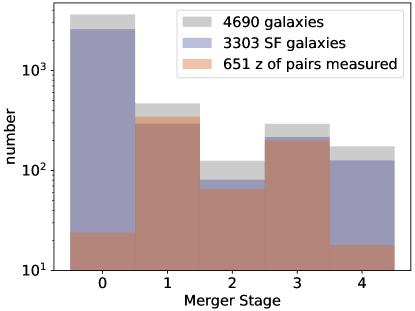
Figure 1: The histogram of the merger stages. The gray color shows the whole sample (N=4,690), the blue color shows the star-forming galaxies (N=3,303), and the red color shows the objects which contains redshift of two members measured and provide

information of projected separation and the difference in the line-of-sight velocity (N=651).

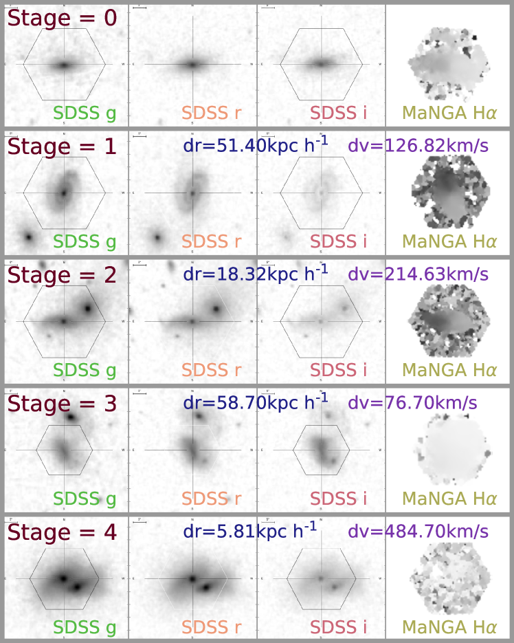
Figure 2: Example of merger stages with input data for classification: the projected separation (dr in kpc $\rm{h}^{-1}$), the velocity difference (dv in km/s), the SDSS $gri$-band image, and the MaNGA H$\alpha$ velocity map.

MaNGA (Bundy et al., 2015; Yan et al., 2016a, b; Wake et al., 2017) is an integral field unit (IFU) survey on the SDSS 2.5 m telescope (Gunn et al., 2006), as part of the SDSS-IV survey (Albareti et al., 2017; Blanton et al., 2017). MaNGA makes use of a modification of the BOSS spectrographs (Smee et al., 2013) to bundle fibers into hexagons (Drory et al., 2015). Each spectrum has a wavelength coverage of 3,500-10,000 and instrumental resolution about 60$km/s$. After dithering, MaNGA data have an effective spatial resolution of 2$\arcsec$.5 (Law et al., 2015), and datacubes are gridded with 0$\arcsec$.5 spaxels. In this work, we use 4,690 galaxies with major-to-minor-axis ratio greater than 0.4 at z$<$0.15 from the MaNGA DR15 version as described in Pan et al. (2019).

Among these 4,690 sample, there are 1,060 merger galaxies and 3,630 non-interacting galaxies or unclassified galaxies according to the classification in Pan et al. (2019). Interactions between galaxies are classified according to the following merger stages:

• Stage 0: non-interacting galaxies, unclassified galaxies, or a potential paired galaxy but without spec-z confirmation for its companion.

• Stage 1: well-separated pairs which do not show any morphology distortion, i.e., incoming pairs, before the first pericenter passage.

• Stage 2: close pairs showing strong signs of interaction, such as tails and bridges, i.e., after the first pericenter passage.

• Stage 3: well-separated pairs, but showing weak morphology, distortion, i.e., approaching the apocenter or just, passing the apocenter.

• Stage 4: two components strongly overlapping with each other and showing strong morphological distortion, i.e., final coalescence phase, or single galaxies with obvious tidal features such as tails and shells, i.e., post-mergers.

According to the visual inspection in Pan et al. (2019), there are 468 galaxies in merger stage 1, 125 galaxies in merger stage 2, 293 galaxies in merger stage 3, and 174 galaxies in merger stage 4. Therefore, there are 1,060 out of the 4,690 sample are classified as interaction galaxies in one of the stages as shown in Figure 1. Among those, 651 objects contain NASA-Sloan Atlas (NSA) redshifts of two members (pairs) measured, which provide information of projected separation ($dr$) and the difference in the line-of-sight velocity ($dv$). Out of these 651 systems, there are 344 galaxies in merger stage 1, 65 galaxies in merger stage 2, 200 galaxies in merger stage 3, and 18 galaxies in merger stage 4. We adopt the values of $dr$ in kpc $\rm{h}^{-1}$ and $dv$ in km/s as input data. For objects without $dr$ and $dv$, we use -999 as input values. As quiescent galaxies do not have prominent features during galaxy-galaxy interaction as star-forming galaxies, in this work, we only focus on the latter. Among the 4690 DR15 galaxuies, 3,303 objects can be selected as star-forming galaxies with $\log$(sSFR/$\rm{yr}^{-1}$)$>$-11 (e.g., McGee et al. 2011; Wetzel et al. 2013; Whitaker et al. 2012, 2014; Lin et al. 2014; Lee et al. 2015; Tomczak et al. 2016; Jian et al. 2018; note that this can only be used in narrow redshift range as MaNGA and SDSS, Donnari et al., 2019, e.g., ). In total, there are 294 galaxies in merger stage 1, 81 galaxies in merger stage 2, 216 galaxies in merger stage 3, and 126 galaxies in merger stage 4 satisfying this criterion. We include all 4,690 MaNGA galaxies in this paper, and limit our sample to 651 objects with redshifts of pairs measured and 3,303 star-forming galaxies for testing purpose.

The visual inspection by Pan et al. (2019) is mainly based on the projected separation ($dr$), the velocity difference ($dv$), the SDSS $gri$-band image, and the MaNGA H$\alpha$ velocity map (for the purpose of redshift identification for the companion, instead of using the kinematic feature). In this paper, we also adopt the above information as input data as shown in Figure 2.

For SDSS images, 50$\arcsec\times$50$\arcsec$ combined images were adopted for visual classification in Pan et al. (2019). Here we decompose these images to gri bands, each with 281 pixels $\times$ 281 pixels, resulting in 78,961 separate inputs. Meanwhile, for MaNGA H$\alpha$ velocity maps, the original image sizes varies from one to another. To be able to create unified datasets for our analysis, we resample each of them on a grid of 50 pixels $\times$ 50 pixels, such that an image contains 2,500 separate inputs. For the whole sample, there are 22 objects without any detection in the MaNGA H$\alpha$ velocity maps, so we choose -9999 for their spaxel values. For low signal-to-noise ratio objects, we still use the measurements from the MaNGA H$\alpha$ velocity maps to include all information.

3 Analysis

3.1 Evaluations

We evaluate the quality of the classification schemes with their performance. First, we defined true positive (TP; a merger source which is classified as merger), true negative (TN: a non-merger source which is not classified as merger), false positive (FP: a non-merger source which is classified as merger), and false negative (FN: a merger source which is not classified as merger). Therefore, the true positive rate (TPR), the true negative rate (TNR), the false positive rate (FPR), and the false negative rate (FNR) are $TPR=TP/(TP+FN)$, $TNR=TN/(TN+FP)$, $FPR=FP/(TN+FP)$, and $FNR=FN/(TP+FN)$, respectively. A good classification will categorize a merger as a merger (TPR) and a non-merger as a non-merger (TNR), rather than a non-merger as a merger (FPR) and a merger as a non-merger (FNR). Accordingly, the result would reach high TPR, high TNR, low FPR, and low FNR. Therefore, high performance can be determined by high accuracy, high precision, high recall, and high F1 score as described below.

• Accuracy: fraction of sources (merger and non-merger) which are classified correctly over all sources.

  $$ACC=\frac{TP+TN}{TP+TN+FP+FN}$$ (1)

• Precision: merger sources which are classified correctly as mergers over all classified mergers.

  $$P=\frac{TP}{TP+FP}$$ (2)

• Recall: merger sources which are classified correctly as mergers over all merger sources.

  $$R=\frac{TP}{TP+FN}$$ (3)

• F1 score: a harmonic mean of the precision and the recall.

  $$F1=2\times\frac{P\times R}{P+R}$$ (4)

3.2 Techniques and Parameters

We use algorithms from Python packages, scikit-learn and XGBoost, to classify galaxy merger stages. In this subsection, we describe several classifiers which are commonly used and applied in this paper including LGBMClassifier, LogisticRegression, DecisionTreeClassifier, RandomForestClassifier, KNeighborsClassifier, MLPClassifier, AdaBoostClassifier, GaussianNB, and XGBoost (Pedregosa et al., 2011; Chen & Guestrin, 2016).

1. LGBMClassifier: a fast and high performance gradient boosting classifier which uses decision tree algorithms. It is a popular learning algorithm which can handle large sample size and takes lower memory. The input parameters are as in below.

   ⬇

   boosting_type=’gbdt’,

   num_leaves=31,

   max_depth=- 1,

   learning_rate=0.1,

   n_estimators=100,

   subsample_for_bin=200000,

   objective=None,

   class_weight=None,

   min_split_gain=0.0,

   min_child_weight=0.001,

   min_child_samples=20,

   subsample=1.0,

   subsample_freq=0,

   colsample_bytree=1.0,

   reg_alpha=0.0,

   reg_lambda=0.0,

   random_state=None,

   n_jobs=- 1,

   importance_type=’split’

   We adopt mostly default parameters of the LGBMClassifier model. We test different combinations of input parameters, but did not find significant differences. The dominant factors of the performance are the selection of input data and the choice of classifications as discussed in the following subsections.

   For other classifiers, we only describe input parameters which are different from default inputs.

2. LogisticRegression: a common model for classification to estimate class probabilities by using a function to train a set of parameter. Here we choose 1000 as the maximum number of iterations, ‘sag’ solver due to the speed, and 0.01 as the tolerance for stopping criteria. Most cases converge before 100 epochs.

3. DecisionTreeClassifier: a predictive modeling classifier which uses decision trees as a predictive model to go from observations about an item represented in the branches to conclude about the item’s target value represented in the leaves. Here we choose 5 as the maximum depth of the tree.

4. RandomForestClassifier: an ensemble learning method for classification which use various decision tree classifiers. Here we choose 5 as the maximum depth, 10 as the number of trees in the forest, and 1 as the number of feature at each split.

5. KNeighborsClassifier: a non-parametric supervised learning method for classification with neighbor searches. The input is the closest K training set, and the output is voted by its K nearest neighbors. Here we choose 3 as the K-neighbors of a point.

6. MLPClassifier: a multi-layer perceptron (MLP) classifier by using neural network. Here we choose 1 as alpha (the strength of the L2 regularization term), and 1000 as the maximum number of iterations. There is one input layer, one hidden layer with 100 neurons, and one output layer. The activation function for the hidden layer is ’relu’, which is the rectified linear unit function. The training stops when the training loss does not improve by more than tol=0.0001 for n_iter_n_change=10 consecutive passes over the training set. Most cases converge before 50 epochs.

7. GaussianNB: Gaussian naive Bayes, which is based on applying Bayes’ theorem with an assumption of the continuous values associated with each class are distributed according to a Gaussian distribution.

8. AdaBoostClassifier: adaptive boosting classifiers, which can be used in conjunction with many other types of learning algorithms. Here the base estimator is DecisionTreeClassifier initialized with maximum depth equal to 1. We choose 50 as the maximum number of estimators at which boosting is terminated.

9. XGBoost: extreme gradient boosting, which is a machine learning algorithms to optimize distributed gradient boosting library and provides a parallel tree boosting learning. Here we use 5 as early stopping rounds which stop while lack of improvement, and 100 number of round of iteration. We choose 10 as the maximum depth of a tree, and 0.3 as ‘eta’, which is the step size shrinkage used in update to prevent overfitting. We set the ‘objective’ to ‘multi:softprob’ to do multiclass classification using the softprob objective, which contains predicted probability of each data point belonging to each class. Most cases converge before 50 epochs.

3.3 Performances

We compare accuracy, precision, recall, and F1 score for different classifiers in Table 1. Three classification cases are discussed as following.

• 5-phase classification ($P_{5}$)

  • $P_{5}^{0}$: non-mergers

  • $P_{5}^{1}$: merger stage 1

  • $P_{5}^{2}$: merger stage 2

  • $P_{5}^{3}$: merger stage 3

  • $P_{5}^{4}$: merger stage 4

• 3-phase classification($P_{3}$)

  • $P_{3}^{0}$: non-mergers

  • $P_{3}^{1}$: well-separated pairs: merger stages 1 and 3

  • $P_{3}^{2}$: very close pairs: merger stages 2 and 4

• 2-phase classification ($P_{2}$)

  • $P_{2}^{0}$: non-mergers

  • $P_{2}^{1}$: mergers: merger stages 1, 2, 3, and 4

We split the galaxy sample to two-third of them as training set and one-third of them as testing set for all classifiers in all cases. We investigate the errors by bootstrapping the sample for each algorithm and estimate their uncertainties. To achieve high performance, we expect to have high accuracy, high precision, high recall, and high F1 score. For galaxy merger stages, we should avoid contamination from non-mergers and wrong classifications. Therefore, the most important goal is to achieve high purity (e.g, Bottrell et al., 2022), which corresponds to high precision score. For multi-classification, we should also check individual precision for each merger stages, that is, merger sources in a specific merger stage which are classified as the correct merger stage over that classified merger stage. For the 5-phase classification, we label $P_{5}^{1}$, $P_{5}^{2}$, $P_{5}^{3}$, and $P_{5}^{4}$ for the individual precision of merger stage 1, 2, 3, and 4, as well as $P_{5}^{0}$ for non-merger precision. For the 3-phase classification, we label $P_{3}^{1}$ and $P_{3}^{2}$ for the individual precision of merger stage 1+3, and 2+4, as well as $P_{3}^{0}$ for non-merger. For the 2-phase classification, we label $P_{2}^{1}$ for mergers, as well as $P_{2}^{0}$ for non-mergers. In Figure 3 and Figure 4, we compare the precision of non-mergers and mergers of 2-phase and 3-phase classification for different classifiers with the original sample (N=4,690). In Figure 5 and Figure 6, we compare the precision of merger stage 1 and 2, as well as merger stage 3 and 4 of 5-phase classification for different classifiers with the original sample (N=4,690).

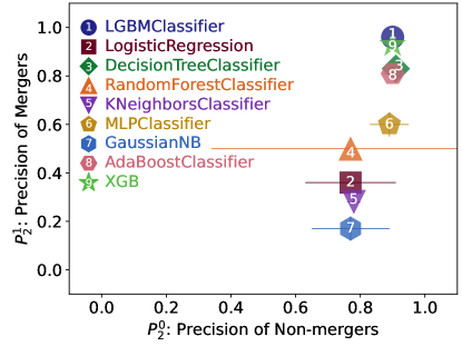
Figure 3: The precision of non-mergers and mergers of 2-phase classification for different classifiers with the original sample (N=4,690).

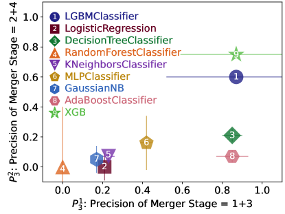
Figure 4: The precision of merger stage 1+3 and 2+4 of 3-phase classification for different classifiers with the original sample (N=4,690).

Figure 5: The precision of merger stage 1 and 2 of 5-phase classification for different classifiers with the original sample (N=4,690).

Figure 6: The precision of merger stage 3 and 4 of 5-phase classification for different classifiers with the original sample (N=4,690).

Figure 7: The precision of non-mergers and mergers of 2-phase classificationfor different classifiers for the original with the rotated sample (N=9,380).

Figure 8: The precision of merger stage 1+3 and 2+4 of 3-phase classificationfor different classifiers for the original with the rotated sample (N=9,380).

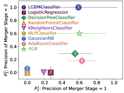
Figure 9: The precision of merger stage 1 and 2 of 5-phase classification for different classifiers for the original with the rotated sample (N=9,380).

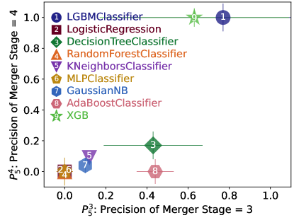
Figure 10: The precision of merger stage 3 and 4 of 5-phase classification for different classifiers for the original with the rotated sample (N=9,380).

For the original SDSS $gri$ images and MaNGA H$\alpha$ velocity maps (N=4,690), we rotate them by 0 and 90 degrees, and we are able to increase their sample size by twice (N=9,380). In this case, we split the training and testing data before rotation to ensure that an image and its rotated counterpart appear in either the same training or the same test sets. In other words, if an image is used for the training set, its rotation is also only used in the training set. As a result, the performance can be improved as shown in Table 1. The precision can be up to 0.85 for 5-phase classification with LGBMClassifier, but have no significant improvement for 3-phase and 2-phase classifications. We also test the sample by more rotated and flipped combinations, but there are no significant changes. Therefore, we keep the combination of the original and one rotated image (0 and 90 degrees). We show the precision of merger stages of 2-phase, 3-phase, and 5-phase classification for different classifiers with the original sample (N=4,690) in Figure 3, Figure 4, Figure 5, and Figure 6, as well as the original with rotated sample (N=9,380) in Figure 7, Figure 8, Figure 9, and Figure 10. As a result, the precisions are improved, especially for 5-phase classification with LGBMClassifier. The 3-phase and 2-phase classifications are slightly improved, but not much as the 5-phase classification as shown in Table 1. To have a consistent comparison, we adopt the original with rotated sample (N=9,380) in the following discussions.

Figure 11, Figure 12, and Figure 13 shows the Receiver Operating Characteristic Curve (ROC) for the best results (N=9,380) of different phase classification with LGBMClassifier. This is to illustrate the diagnostic ability of the classifier system by plotting the true positive rate (also known as recall or sensitivity) against the false positive rate (also known as probability of false alarm) at various threshold settings. For multiclass problems, ROC curves and Area Under the ROC scores (AUROC; ideal case is equal to 1) represent each class versus the rest individually. Here we show that the scores can reach high performance ($\gtrsim$0.80) for most cases.

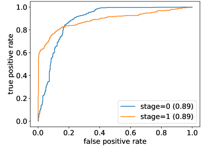
Figure 11: The Receiver Operating Characteristic Curve (ROC) for 2-phase classification. The values show the Area Under the Receiver Operating Characteristic Curve score (AUROC) for the original with rotated sample (N=9,380) with LGBMClassifier.

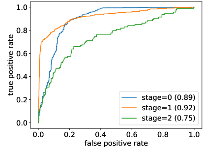
Figure 12: The Receiver Operating Characteristic Curve (ROC) for 3-phase classification. The values show the Area Under the Receiver Operating Characteristic Curve score (AUROC) for the original with rotated sample (N=9,380) with LGBMClassifier.

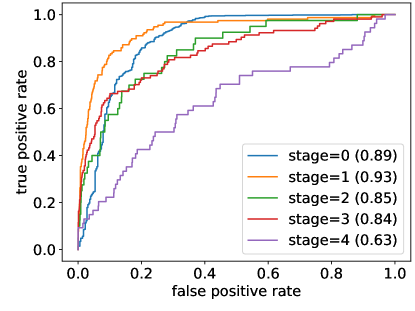
Figure 13: The Receiver Operating Characteristic Curve (ROC) for 5-phase classification. The values show the Area Under the Receiver Operating Characteristic Curve score (AUROC) for the original with rotated sample (N=9,380) with LGBMClassifier.

We show the feature importance to indicate the importance of each input feature in Figure 14, Figure 15, and Figure 16 for the best results (N=9,380) with LGBMClassifier. In the input parameters of LGBMClassifier, we choose ‘split’ importance type, which calculates numbers of times the feature is used in the tree-structured nodes for each feature. For SDSS $gri$ images and MaNGA H$\alpha$ velocity map, the number of times in the nodes are calculated for each spaxel. We find that the spaxels in the center are more important than the outskirts, but the results are similar if we rotate, flip, or translate the image by few pixels. To investigate the effect of the entire image size, we sum up the total numbers of times in the tree-structured nodes for all spaxels. Therefore, there are six features: SDSS $g$-band image ($g$), SDSS $r$-band image ($r$), SDSS $i$-band image($i$), MaNGA H$\alpha$ velocity map (H$\alpha$), the projected separation ($dr$), and the velocity difference ($dv$). As a sanitary test, we resample the images ($g$, $r$, $i$, and H$\alpha$) to the same scale (e.g., 100 pixels$\times$100 pixels), as well as duplicate the values of $dr$ and $dv$ to the same number of scale (e.g, 100$\times$100). As a result, we find that the ranking of the six features is unchanged, and there are no significant differences between the original and the resampled feature importance. This indicates that the image size is independent of the feature importance, and the summation of the total numbers of times with all spaxels for each single image is feasible.

As shown in Figure 14, Figure 15, and Figure 16, the top three important features are SDSS $gri$ images. Among them, SDSS $i$-band image is the most important feature for all 2-, 3-, and 5-phase classifications. The fourth important feature is H$\alpha$, the fifth important feature is $dr$ , the sixth important feature is $dv$. The differences among different stages, which calculated the cumulative feature importance for each stage individually, are not very significant. This is consistent with our expectation because the merger stages were mainly classified by the SDSS imaging.

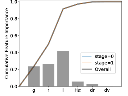
Figure 14: Cumulative feature importance plot for the original with the rotated sample (N=9,380) with LGBMClassifier for individual stages and overall classifications of 2-phase classification.

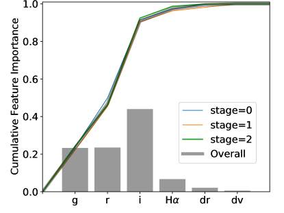
Figure 15: Cumulative feature importance plot for the original with the rotated sample (N=9,380) with LGBMClassifier for individual stages and overall classifications of 3-phase classification.

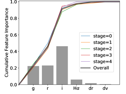
Figure 16: Cumulative feature importance plot for the original with the rotated sample (N=9,380) with LGBMClassifier for individual stages and overall classifications of 5-phase classification.

4 Discussion

4.1 Can galaxy interactions be identified?

In this work we use LGBMClassifier, LogisticRegression, DecisionTreeClassifier, RandomForestClassifier, KNeighborsClassifier, MLPClassifier, AdaBoostClassifier, GaussianNB, and XGBoost algorithms to identify interacting galaxies.

For the 2-phase classification, it is not difficult for some classifiers to reach high accuracy (ACC), high precision (P), high recall (R), and high F1 (F1) score as shown in Table 1. We can reach high performance with 0.91 in accuracy, 0.93 in precision (purity), 0.81 in recall (completeness), and 0.85 in F1 score. The good performance of binary classification for merging galaxies is also discussed in Pearson et al. (2019, 0.53-0.92 in accuracy), Ferreira et al. (2020, 0.90 in accuracy), Nevin et al. (2021, 0.80 in accuracy and 0.90 in precision), and Bottrell et al. (2022, 0.93 in purity and 0.93 in completeness based on noiseless data from simulations). The most important score in 2-phase classification is the $P_{2}^{1}$ value, which is derived by the merger sources which are classified correctly as mergers over all classified mergers. There are several classifiers (LGBMClassifier, XGBoost, DecisionTreeClassifier, and AdaBoostClassifier) can achieve high $P_{2}^{1}$ values ($\gtrsim$0.80) with the original sources (N=4,690) as shown in Figure 3. In particular, LGBMClassifier and XGBoost can achieve very high $P_{2}^{1}$ values ($\gtrsim$0.95). This may suggest that merger features of interacting galaxies are easier to be identified by tree-structured classifiers than others, especially with boosting trees.

From the 4,690 galaxies, we select 3,303 star-forming galaxies with $\log$(sSFR/$\rm{yr}^{-1}$)$>$-11, and find that the precision can be improved by 5 to 10 % even though the sample size is slightly decreased. One reason might be that MaNGA H$\alpha$ velocity maps are mainly available for star-forming galaxies or galaxies above some gas fraction, and are blank or low values for gas-poor galaxies which lack spaxels with sufficient signal-to-noise ratio. Nevertheless, the contribution of H$\alpha$ velocity maps is less significant than the SDSS $gri$-band image as shown in Figure 14 and Figure 17. Another reason is that our classification scheme is not easy to distinguish the 5-phase mergers for dry mergers (e.g., Lotz et al., 2010), which shows fewer distortions on the images anyway. On the other hand, this would not be a problem for 2-phase or 3-phase mergers, so the differences are less significant. Therefore, visual classification for wet mergers is more reliable than dry mergers, and interaction features are more obvious for star-forming galaxies.This can be consistent with previous finding that classification performance based on both imaging and stellar kinematics tends to increase with high gas fraction (Lotz et al., 2011; Bottrell et al., 2022).

4.2 Can galaxy merger stages be classified?

For the 5-phase classification with original sample (N=4,690), the accuracy (ACC) and the precision of non-mergers $P_{5}^{0}$ can reach to high scores ($\gtrsim$0.80 and $\gtrsim$0.90, respectively) for several classifiers (LGBMClassifier, DecisionTreeClassifier, AdaBoostClassifier, and XGBoost). If we consider the Top-N accuracy, it can be up to 0.85, 0.92, 9.95, 0.98, 1.00 for N=1 to N=5 cases. However, the averaged precision (P) and the precision of each stage ($P_{5}^{0}$, $P_{5}^{1}$, $P_{5}^{2}$, $P_{5}^{3}$, and $P_{5}^{4}$) are less than 0.60 for all classifiers, perhaps because of the degeneracy of the stages which are not easy to be classified by the original sample size.

We combine similar morphology to the same classification in the 3-phase classification, which contains non-merger, 1+3 merger stage for well-separated sources, and 2+4 merger stage for very close pairs. Table 1 shows that the precision of merger stage 1+3 ($P_{3}^{1}$) and merger stage 2+4 ($P_{3}^{2}$) can be improved. For XGBoost and LGBMClassifier classifiers, the precision of non-mergers and stage 1+3 can reach high scores ($\gtrsim$0.85), and the precision of non-mergers and stage 2+4 is also improved ($\gtrsim$0.60) as shown in Figure 4.

In order to improve performance of the 5-phase classification, we adopt the combination of original and rotated images. In this work, the physical parameters,such as stellar mass, star formation rate, and interactions between galaxies, would not be affected if we rotate or flip the images. Therefore, we are able to increase the sample size by twice (N=9,380) as shown in Table 1. We find that the performance of the scores are improved, especially for LGBMClassifier classifiers. In Figure 9 and Figure 10, the averaged precision (P) and the precision of non-mergers, stage 2 and stage 4 ($P_{5}^{0}$, $P_{5}^{2}$, and $P_{5}^{4}$) can reach high scores ($\gtrsim$0.90), and the precision of stage 1 and stage 3 ($P_{5}^{1}$ and $P_{5}^{3}$) is also improved ($\gtrsim$0.60).

We find that LGBMClassifier can provide better performances, especially for good precision, among all classifiers in this work. We have tested different input parameters of LGBMClassifier, but there is no significant improvement for the performance. In some cases, XGBoost, DecisionTreeClassifier, and AdaBoostClassifier can also provide good performances. We test the classifiers by tuning their input parameters, and the above tree-structured classifiers show better performances in most cases. One reason might be that the whole spaxels of the image data are not the best hyperparameters for other models. Nevertheless, we show that the physical features of interacting galaxies are easier to be classified by tree-structured classifiers, especially with gradient boosting trees such as XGBoost and LGBMClassifier. In general, the differences can be explained by the limit of the algorithm, the choice of our input parameters, and the characteristic of our data. While it may be possible to find a more sophisticate algorithms to improve the performance, our results show that we are able to classify galaxy mergers with good performance by using the ML techniques tested in this work.

4.3 What input data and features are important in galaxy interaction?

We show the cumulative feature importance of the input data in Figure  14, Figure  15, and Figure  16. The top three important features are SDSS images ($i>g\simeq r$). The contribution from MaNGA H$\alpha$ velocity map (H$\alpha$), the projected separation ($dr$), and line-of-sight velocity difference ($dv$) can also improve the performance. As discussed in Section 4.1, MaNGA H$\alpha$ velocity maps (H$\alpha$) are mainly available for star-forming galaxies or galaxies above some gas fraction. Moreover, $dr$ and $dv$ values are only available when the redshift of two members (pairs) are measured. It is possible that SDSS images are top features because they are the only data that all the galaxies have. However, if we limit the sample size to objects with available H$\alpha$ velocity maps, or star forming galaxies with $\log$(sSFR/$\rm{yr}^{-1}$)$>$-11 (N=3,303; high signal-to-noise ratio of H$\alpha$), or the sample with the projected separation and line-of-sight velocity difference (N=651; available $dr$ and $dv$), the feature importance plots are only slightly different, and the top features are still SDSS images ($g$, $r$, and $i$). We also find that the differences of cumulative feature importance among various stages are not significant, so the overall curve is sufficient to describe the features. This result is consistent with our expectation, that is, SDSS images are the dominant features to distinguish galaxy interactions.

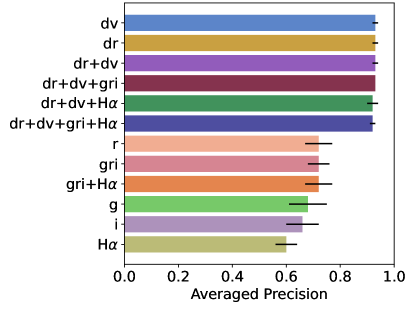
Figure 17: The averaged precision of 2-phase classification for different input data for the original with the rotated sample (N=9,380).

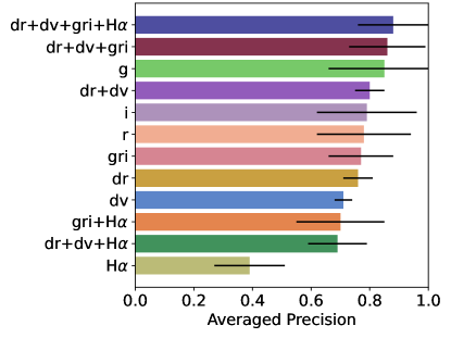
Figure 18: The averaged precision of 3-phase classification for different input data for the original with the rotated sample (N=9,380).

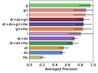
Figure 19: The averaged precision of 5-phase classification for different input data for the original with the rotated sample (N=9,380).

In order to investigate the input features individually, we test the performance of different combinations of input data (the projected separation, the velocity difference, the SDSS $gri$-band image, and the MaNGA H$\alpha$ velocity map) for original with the rotated sample (N=9,380) by LGBMClassifier in Table 2, Figure 17, Figure 18, and Figure 19. In general, the most important features are SDSS $gri$ images, and the contribution from MaNGA H$\alpha$ velocity map, the projected separation, as well as line-of-sight velocity difference can also improve the performance by 0-20%. Because $dr$ and $dv$ only exist for galaxies with spectroscopic neighbors, so they should alone yield all galaxies in the pair phase wherever both galaxies have spectra. If we remove the information of $dr$ and $dv$, the performance is decreased, especially for 2-phase classification. Moreover, $dr$ or $dv$ alone can reach high performance for 2-phase classification, but the change in performance is not for 3-phase and 5-phase classifications. This suggests that $dr$ and $dv$ are sufficient to identify galaxy mergers, but additional imaging data are required if detailed merging stages are investigated. For 3-phase classification, the performance is less affected if the SDSS $gri$-band images are still included. The $g$-, $r$-, and $i$-band images are highly correlated to each other. If we remove one of them, the performance is slightly decreased but not significant compared to the case which we include all of the three $gri$-band. As a result, we show that the contributions from SDSS images are important. For 2-phase classification in Figure 17, $dr$ or $dv$ alone can already achieve a high precision score ($\gtrsim$0.90). This can be explained by that these two values are only available when redshift of pairs measured, so the information is already sufficient to identify galaxy mergers. However, for 3-phase classification in Figure 18 or 5-phase classification in Figure 19, it is obvious to see that SDSS $gri$-band image and the MaNGA H$\alpha$ velocity map are required. Besides, it is interesting that the information from $g$, $r$, $i$-image alone can each reach $\sim$70% precision, and even better than some other combinations. This implies that a single-band SDSS image for MaNGA galaxies can provide sufficient photometric quality to reveal the most important information and low-surface brightness features about galaxy interactions (e.g., Bottrell et al., 2019; Ćiprijanović et al., 2021; Bickley et al., 2021; Ferreira et al., 2020). In particular, SDSS $i$-band image is the top feature in Figure 14, Figure 15, and Figure 16, and single $g$-band SDSS image can achieve a high precision score ($\gtrsim$0.90) for 3-phase and 5-phase classifications as shown in Figure 18 and Figure 19. This implies that single SDSS band image might be sufficient to distinguish detailed interacting features of galaxies, but further investigations are required.

If we remove MaNGA H$\alpha$ velocity map from the input data as shown in Table 2, the performance might be decreased but have little changes ($<$5%) for 2-phase, 3-phase, and 5-phase classifications. Bottrell et al. (2022) shows that stellar kinematic data has little to offer in compliment to imaging for merger remnant identification by using TNG100 cosmological hydrodynamical simulation. Besides, Nevin et al. (2021) investigate the importance of stellar kinematics, and find 0.80 in accuracy and 0.90 in precision for major merger classification. McElroy et al. (2022) use stellar kinematics on the role of field-of-view limitations to classify mergers into different stages, and find 0.40-0.79 completeness in pairs, and 0.97-1.00 completeness in the merging and post-coalescent phases. In our work, IFU data can still provide redshift information (i.e, $dv$, the difference in the line-of-sight velocity) to improve the performance of merger stage classification, especially for 2-phase classification. However, the kinematic information in the velocity map provides little contribution to the current merger stage classification. On the other hand, the image and the velocity information alone can already achieve high performance. There are many available IFU data from MaNGA, but the current choice of inputs (i. e., projected separation, the velocity difference, all the spaxels of the SDSS $gri$-band image and the MaNGA H$\alpha$ velocity map) are sufficient to identify galaxy merger and their stages with a sample size of 4,690 galaxies with the state-of-the-art classifiers and the rotation technique. It is possible that other measurements in the IFU data can provide more information, such as kinematics of galaxy interactions derived from other MaNGA data. If the dataset is with different quality (i.e., resolution or signal-to-noise ratio), it is also possible that additional IFU data, such as asymmetries and other non-parametric map characteristics, become important information. Moreover, we check our false positive sources, which are non-merger galaxies classified by visual inspection while merger galaxies classified by machine learning. There are some suspicious cases, but it is difficult to conclude whether they turn out to be possible interacting galaxies. Therefore, it is possible that the abundant IFU data from MaNGA may unveil additional information by using unsupervised or other ML techniques.. In this work, we show that the current parameters are already enough to classify galaxy merger stages without visual inspection. This will be helpful for us to understand galaxy interaction with a larger sample in the future all-sky surveys.

5 Summary

In this paper, we have identified MaNGA merger stages by machine learning techniques. Our main findings are as follows.

1. For 2-phase classification, the performance can be high (precision$>$0.90) with LGBMClassifier. In general, merger features of interacting galaxies are easy to be identified by tree-structured classifiers, especially with gradient boosting trees.

2. Sample size can be increased by the combination of the original and rotated images. Then 5-phase classification can also be good (precision$>$0.85).

3. The most important features are SDSS $gri$ images, and single-band SDSS image can already provide most information about galaxy interactions. The contribution from MaNGA H$\alpha$ velocity map, the projected separation, and line-of-sight velocity difference can also improve the performance by 0-20%.

4. The kinematic information in the velocity map provides less contribution to the current merger stage classification. On the other hand, the image and the velocity information alone can already achieve high performance.

5. These results can apply to the entire MaNGA data as well as future all-sky surveys.

classifier	ACC	P	R	F1	$P^{0}$	$P^{1}$	$P^{2}$	$P^{3}$	$P^{4}$
5-phase Classification (original with rotated sample, N=9,380)
LGBMClassifier	0.85$\pm$0.01	0.85$\pm$0.13	0.39$\pm$0.01	0.40$\pm$0.02	0.89$\pm$0.01	0.59$\pm$0.03	1.00$\pm$0.45	0.77$\pm$0.06	1.00$\pm$0.49
LogisticRegression	0.77$\pm$0.01	0.21$\pm$0.02	0.20$\pm$0.00	0.18$\pm$0.00	0.78$\pm$0.01	0.27$\pm$0.10	0.00$\pm$0.00	0.00$\pm$0.00	0.00$\pm$0.00
DecisionTreeClassifier	0.84$\pm$0.02	0.47$\pm$0.08	0.38$\pm$0.02	0.40$\pm$0.03	0.90$\pm$0.01	0.55$\pm$0.06	0.29$\pm$0.19	0.43$\pm$0.10	0.17$\pm$0.24
RandomForestClassifier	0.77$\pm$0.01	0.15$\pm$0.00	0.20$\pm$0.00	0.17$\pm$0.00	0.77$\pm$0.01	0.00$\pm$0.00	0.00$\pm$0.00	0.00$\pm$0.00	0.00$\pm$0.00
KNeighborsClassifier	0.75$\pm$0.02	0.24$\pm$0.01	0.21$\pm$0.01	0.19$\pm$0.01	0.78$\pm$0.01	0.19$\pm$0.03	0.00$\pm$0.03	0.12$\pm$0.03	0.09$\pm$0.04
MLPClassifier	0.77$\pm$0.16	0.15$\pm$0.03	0.20$\pm$0.02	0.17$\pm$0.01	0.77$\pm$0.03	0.00$\pm$0.07	0.00$\pm$0.02	0.00$\pm$0.07	0.00$\pm$0.00
GaussianNB	0.06$\pm$0.01	0.15$\pm$0.02	0.24$\pm$0.02	0.06$\pm$0.01	0.58$\pm$0.07	0.00$\pm$0.00	0.06$\pm$0.02	0.10$\pm$0.02	0.04$\pm$0.01
AdaBoostClassifier	0.83$\pm$0.01	0.43$\pm$0.05	0.39$\pm$0.02	0.41$\pm$0.03	0.89$\pm$0.01	0.63$\pm$0.07	0.18$\pm$0.15	0.44$\pm$0.09	0.00$\pm$0.09
XGB	0.85$\pm$0.01	0.74$\pm$0.13	0.41$\pm$0.01	0.44$\pm$0.02	0.89$\pm$0.01	0.60$\pm$0.05	0.60$\pm$0.31	0.63$\pm$0.10	1.00$\pm$0.46
5-phase Classification (original sample, N=4,690)
LGBMClassifier	0.85$\pm$0.01	0.72$\pm$0.08	0.38$\pm$0.02	0.40$\pm$0.02	0.90$\pm$0.01	0.62$\pm$0.04	1.00$\pm$0.33	0.42$\pm$0.09	0.67$\pm$0.36
LogisticRegression	0.77$\pm$0.01	0.15$\pm$0.03	0.20$\pm$0.00	0.17$\pm$0.00	0.77$\pm$0.01	0.00$\pm$0.17	0.00$\pm$0.00	0.00$\pm$0.00	0.00$\pm$0.00
DecisionTreeClassifier	0.83$\pm$0.00	0.41$\pm$0.03	0.37$\pm$0.01	0.38$\pm$0.02	0.90$\pm$0.01	0.61$\pm$0.05	0.05$\pm$0.08	0.33$\pm$0.09	0.16$\pm$0.08
RandomForestClassifier	0.77$\pm$0.01	0.15$\pm$0.00	0.20$\pm$0.00	0.17$\pm$0.00	0.77$\pm$0.01	0.00$\pm$0.00	0.00$\pm$0.00	0.00$\pm$0.00	0.00$\pm$0.00
KNeighborsClassifier	0.74$\pm$0.01	0.22$\pm$0.02	0.20$\pm$0.02	0.19$\pm$0.02	0.77$\pm$0.01	0.21$\pm$0.06	0.00$\pm$0.05	0.06$\pm$0.02	0.06$\pm$0.03
MLPClassifier	0.77$\pm$0.16	0.15$\pm$0.05	0.20$\pm$0.02	0.17$\pm$0.03	0.77$\pm$0.03	0.00$\pm$0.27	0.00$\pm$0.02	0.00$\pm$0.05	0.00$\pm$0.01
GaussianNB	0.08$\pm$0.02	0.20$\pm$0.03	0.26$\pm$0.03	0.06$\pm$0.01	0.72$\pm$0.07	0.17$\pm$0.07	0.06$\pm$0.03	0.00$\pm$0.04	0.03$\pm$0.01
AdaBoostClassifier	0.82$\pm$0.01	0.37$\pm$0.02	0.34$\pm$0.02	0.35$\pm$0.02	0.90$\pm$0.01	0.56$\pm$0.04	0.06$\pm$0.06	0.29$\pm$0.05	0.07$\pm$0.06
XGB	0.85$\pm$0.01	0.55$\pm$0.06	0.39$\pm$0.02	0.42$\pm$0.02	0.90$\pm$0.01	0.64$\pm$0.04	0.38$\pm$0.15	0.43$\pm$0.08	0.40$\pm$0.34
3-phase Classification (original with rotated sample, N=9,380)
LGBMClassifier	0.89$\pm$0.01	0.88$\pm$0.12	0.59$\pm$0.01	0.62$\pm$0.03	0.89$\pm$0.01	0.88$\pm$0.03	0.88$\pm$0.33
LogisticRegression	0.77$\pm$0.01	0.38$\pm$0.04	0.34$\pm$0.01	0.31$\pm$0.01	0.78$\pm$0.01	0.35$\pm$0.11	0.00$\pm$0.07
DecisionTreeClassifier	0.88$\pm$0.01	0.72$\pm$0.04	0.59$\pm$0.01	0.62$\pm$0.02	0.89$\pm$0.01	0.84$\pm$0.03	0.43$\pm$0.13
RandomForestClassifier	0.77$\pm$0.01	0.26$\pm$0.10	0.33$\pm$0.00	0.29$\pm$0.00	0.77$\pm$0.01	0.00$\pm$0.30	0.00$\pm$0.00
KNeighborsClassifier	0.74$\pm$0.01	0.38$\pm$0.02	0.35$\pm$0.02	0.34$\pm$0.02	0.78$\pm$0.01	0.24$\pm$0.03	0.12$\pm$0.05
MLPClassifier	0.65$\pm$0.14	0.44$\pm$0.09	0.50$\pm$0.06	0.44$\pm$0.07	0.90$\pm$0.05	0.34$\pm$0.21	0.08$\pm$0.04
GaussianNB	0.07$\pm$0.01	0.29$\pm$0.05	0.33$\pm$0.01	0.05$\pm$0.01	0.61$\pm$0.12	0.20$\pm$0.14	0.06$\pm$0.01
AdaBoostClassifier	0.87$\pm$0.01	0.64$\pm$0.02	0.56$\pm$0.01	0.59$\pm$0.01	0.89$\pm$0.01	0.85$\pm$0.03	0.17$\pm$0.04
XGB	0.89$\pm$0.01	0.89$\pm$0.09	0.59$\pm$0.01	0.63$\pm$0.01	0.89$\pm$0.01	0.88$\pm$0.03	0.89$\pm$0.26
3-phase Classification (original sample, N=4,690)
LGBMClassifier	0.89$\pm$0.01	0.79$\pm$0.12	0.58$\pm$0.02	0.60$\pm$0.02	0.90$\pm$0.01	0.87$\pm$0.02	0.60$\pm$0.35
LogisticRegression	0.77$\pm$0.01	0.33$\pm$0.03	0.33$\pm$0.00	0.30$\pm$0.00	0.77$\pm$0.01	0.21$\pm$0.09	0.00$\pm$0.00
DecisionTreeClassifier	0.87$\pm$0.01	0.65$\pm$0.02	0.60$\pm$0.01	0.62$\pm$0.02	0.91$\pm$0.01	0.85$\pm$0.04	0.21$\pm$0.05
RandomForestClassifier	0.77$\pm$0.01	0.26$\pm$0.13	0.33$\pm$0.00	0.29$\pm$0.00	0.77$\pm$0.01	0.00$\pm$0.40	0.00$\pm$0.00
KNeighborsClassifier	0.74$\pm$0.02	0.36$\pm$0.02	0.34$\pm$0.02	0.33$\pm$0.02	0.78$\pm$0.01	0.23$\pm$0.03	0.07$\pm$0.03
MLPClassifier	0.76$\pm$0.19	0.46$\pm$0.06	0.39$\pm$0.02	0.39$\pm$0.05	0.80$\pm$0.04	0.42$\pm$0.18	0.16$\pm$0.03
GaussianNB	0.08$\pm$0.03	0.31$\pm$0.05	0.33$\pm$0.01	0.06$\pm$0.01	0.70$\pm$0.08	0.17$\pm$0.09	0.05$\pm$0.01
AdaBoostClassifier	0.87$\pm$0.01	0.61$\pm$0.03	0.55$\pm$0.02	0.57$\pm$0.02	0.90$\pm$0.01	0.85$\pm$0.04	0.07$\pm$0.08
XGB	0.89$\pm$0.01	0.84$\pm$0.09	0.59$\pm$0.01	0.62$\pm$0.01	0.90$\pm$0.01	0.87$\pm$0.02	0.75$\pm$0.28
2-phase Classification (original with rotated sample, N=9,380)
LGBMClassifier	0.90$\pm$0.00	0.92$\pm$0.01	0.79$\pm$0.01	0.84$\pm$0.01	0.89$\pm$0.01	0.95$\pm$0.01
LogisticRegression	0.77$\pm$0.01	0.65$\pm$0.06	0.51$\pm$0.01	0.47$\pm$0.01	0.78$\pm$0.01	0.52$\pm$0.11
DecisionTreeClassifier	0.89$\pm$0.01	0.91$\pm$0.03	0.78$\pm$0.01	0.83$\pm$0.01	0.89$\pm$0.01	0.92$\pm$0.06
RandomForestClassifier	0.77$\pm$0.01	0.39$\pm$0.23	0.50$\pm$0.00	0.44$\pm$0.00	0.77$\pm$0.01	0.00$\pm$0.46
KNeighborsClassifier	0.60$\pm$0.09	0.63$\pm$0.10	0.69$\pm$0.07	0.58$\pm$0.08	0.93$\pm$0.04	0.34$\pm$0.20
MLPClassifier	0.77$\pm$0.27	0.47$\pm$0.09	0.50$\pm$0.01	0.44$\pm$0.13	0.77$\pm$0.10	0.17$\pm$0.16
GaussianNB	0.78$\pm$0.22	0.39$\pm$0.09	0.50$\pm$0.00	0.44$\pm$0.10	0.78$\pm$0.09	0.00$\pm$0.09
AdaBoostClassifier	0.89$\pm$0.01	0.87$\pm$0.03	0.79$\pm$0.01	0.82$\pm$0.01	0.89$\pm$0.01	0.85$\pm$0.05
XGB	0.90$\pm$0.01	0.91$\pm$0.01	0.80$\pm$0.02	0.84$\pm$0.02	0.90$\pm$0.01	0.93$\pm$0.02
2-phase Classification (original sample, N=4,690)
LGBMClassifier	0.91$\pm$0.01	0.93$\pm$0.01	0.81$\pm$0.01	0.85$\pm$0.01	0.90$\pm$0.01	0.96$\pm$0.01
LogisticRegression	0.77$\pm$0.01	0.56$\pm$0.07	0.50$\pm$0.01	0.45$\pm$0.01	0.77$\pm$0.01	0.36$\pm$0.14
DecisionTreeClassifier	0.89$\pm$0.01	0.87$\pm$0.01	0.81$\pm$0.01	0.84$\pm$0.01	0.91$\pm$0.01	0.83$\pm$0.02
RandomForestClassifier	0.77$\pm$0.01	0.64$\pm$0.21	0.50$\pm$0.00	0.44$\pm$0.01	0.77$\pm$0.01	0.50$\pm$0.43
KNeighborsClassifier	0.72$\pm$0.02	0.53$\pm$0.01	0.51$\pm$0.01	0.50$\pm$0.01	0.78$\pm$0.01	0.28$\pm$0.02
MLPClassifier	0.77$\pm$0.16	0.69$\pm$0.02	0.50$\pm$0.05	0.44$\pm$0.09	0.77$\pm$0.05	0.60$\pm$0.06
GaussianNB	0.77$\pm$0.26	0.47$\pm$0.06	0.50$\pm$0.01	0.44$\pm$0.14	0.77$\pm$0.05	0.17$\pm$0.12
AdaBoostClassifier	0.88$\pm$0.01	0.85$\pm$0.02	0.80$\pm$0.02	0.82$\pm$0.02	0.90$\pm$0.01	0.81$\pm$0.03
XGB	0.91$\pm$0.01	0.92$\pm$0.01	0.82$\pm$0.02	0.85$\pm$0.02	0.90$\pm$0.01	0.93$\pm$0.01

Table 1: Numbers of accuracy, precision, recall, F1 score, and individual precision of different classifiers. The uncertainties are derived by bootstrapping.

data	ACC	P	R	F1	$P^{0}$	$P^{1}$	$P^{2}$	$P^{3}$	$P^{4}$
5-phase Classification (original with rotated sample, N=9,380)
dr+dv+$gri$+H$\alpha$	0.85$\pm$0.01	0.85$\pm$0.13	0.39$\pm$0.01	0.40$\pm$0.02	0.89$\pm$0.01	0.59$\pm$0.03	1.00$\pm$0.45	0.77$\pm$0.06	1.00$\pm$0.49
dr+dv+$gri$	0.86$\pm$0.01	0.85$\pm$0.10	0.40$\pm$0.01	0.42$\pm$0.02	0.89$\pm$0.01	0.61$\pm$0.05	1.00$\pm$0.45	0.75$\pm$0.07	1.00$\pm$0.50
dr+dv+H$\alpha$	0.85$\pm$0.01	0.68$\pm$0.09	0.39$\pm$0.01	0.41$\pm$0.02	0.89$\pm$0.01	0.61$\pm$0.05	0.40$\pm$0.32	0.52$\pm$0.10	1.00$\pm$0.34
$gri$+H$\alpha$	0.78$\pm$0.01	0.84$\pm$0.14	0.22$\pm$0.01	0.22$\pm$0.01	0.78$\pm$0.01	0.40$\pm$0.33	1.00$\pm$0.49	1.00$\pm$0.30	1.00$\pm$0.50
dr+dv	0.85$\pm$0.01	0.71$\pm$0.05	0.42$\pm$0.02	0.47$\pm$0.02	0.89$\pm$0.01	0.62$\pm$0.03	0.50$\pm$0.14	0.55$\pm$0.07	1.00$\pm$0.32
dr	0.84$\pm$0.01	0.54$\pm$0.08	0.39$\pm$0.02	0.43$\pm$0.03	0.88$\pm$0.01	0.59$\pm$0.03	0.30$\pm$0.11	0.48$\pm$0.10	0.44$\pm$0.38
dv	0.84$\pm$0.01	0.52$\pm$0.04	0.39$\pm$0.02	0.42$\pm$0.02	0.88$\pm$0.01	0.60$\pm$0.04	0.32$\pm$0.08	0.59$\pm$0.09	0.19$\pm$0.15
$gri$	0.78$\pm$0.01	0.89$\pm$0.20	0.22$\pm$0.01	0.22$\pm$0.01	0.78$\pm$0.01	0.67$\pm$0.29	1.00$\pm$0.30	1.00$\pm$0.46	1.00$\pm$0.46
$g$	0.78$\pm$0.01	0.96$\pm$0.18	0.22$\pm$0.01	0.22$\pm$0.01	0.78$\pm$0.01	1.00$\pm$0.38	1.00$\pm$0.46	1.00$\pm$0.49	1.00$\pm$0.49
$r$	0.78$\pm$0.01	0.88$\pm$0.19	0.22$\pm$0.01	0.22$\pm$0.01	0.78$\pm$0.01	0.60$\pm$0.39	1.00$\pm$0.46	1.00$\pm$0.00	1.00$\pm$0.49
$i$	0.78$\pm$0.01	0.81$\pm$0.19	0.22$\pm$0.01	0.22$\pm$0.02	0.78$\pm$0.01	0.75$\pm$0.33	0.50$\pm$0.49	1.00$\pm$0.49	1.00$\pm$0.40
H$\alpha$	0.77$\pm$0.01	0.21$\pm$0.04	0.20$\pm$0.00	0.18$\pm$0.01	0.78$\pm$0.01	0.27$\pm$0.14	0.00$\pm$0.00	0.00$\pm$0.10	0.00$\pm$0.00
3-phase Classification (original with rotated sample, N=9,380)
dr+dv+$gri$+H$\alpha$	0.89$\pm$0.01	0.88$\pm$0.12	0.59$\pm$0.01	0.62$\pm$0.03	0.89$\pm$0.01	0.88$\pm$0.03	0.88$\pm$0.33
dr+dv+$gri$	0.89$\pm$0.01	0.86$\pm$0.13	0.58$\pm$0.01	0.60$\pm$0.02	0.89$\pm$0.01	0.86$\pm$0.02	0.83$\pm$0.40
dr+dv+H$\alpha$	0.88$\pm$0.00	0.69$\pm$0.10	0.57$\pm$0.01	0.59$\pm$0.02	0.89$\pm$0.01	0.86$\pm$0.03	0.33$\pm$0.29
$gri$+H$\alpha$	0.78$\pm$0.01	0.70$\pm$0.15	0.35$\pm$0.01	0.33$\pm$0.01	0.78$\pm$0.01	0.73$\pm$0.23	0.60$\pm$0.39
dr+dv	0.89$\pm$0.01	0.80$\pm$0.05	0.60$\pm$0.02	0.64$\pm$0.02	0.89$\pm$0.00	0.90$\pm$0.01	0.59$\pm$0.14
dr	0.88$\pm$0.01	0.76$\pm$0.05	0.58$\pm$0.02	0.62$\pm$0.02	0.89$\pm$0.01	0.89$\pm$0.02	0.50$\pm$0.14
dv	0.88$\pm$0.01	0.71$\pm$0.03	0.57$\pm$0.01	0.61$\pm$0.01	0.89$\pm$0.01	0.89$\pm$0.02	0.34$\pm$0.08
$gri$	0.78$\pm$0.01	0.77$\pm$0.11	0.35$\pm$0.01	0.33$\pm$0.01	0.78$\pm$0.01	0.53$\pm$0.23	1.00$\pm$0.40
$g$	0.78$\pm$0.01	0.85$\pm$0.19	0.36$\pm$0.01	0.34$\pm$0.02	0.78$\pm$0.01	0.77$\pm$0.29	1.00$\pm$0.46
$r$	0.78$\pm$0.01	0.78$\pm$0.16	0.35$\pm$0.01	0.34$\pm$0.01	0.78$\pm$0.01	0.56$\pm$0.21	1.00$\pm$0.46
$i$	0.78$\pm$0.01	0.79$\pm$0.18	0.35$\pm$0.01	0.33$\pm$0.01	0.78$\pm$0.01	0.60$\pm$0.18	1.00$\pm$0.49
H$\alpha$	0.77$\pm$0.01	0.39$\pm$0.12	0.34$\pm$0.00	0.31$\pm$0.01	0.78$\pm$0.01	0.39$\pm$0.12	0.00$\pm$0.30
2-phase Classification (original with rotated sample, N=9,380)
dr+dv+$gri$+H$\alpha$	0.90$\pm$0.00	0.92$\pm$0.01	0.79$\pm$0.01	0.84$\pm$0.01	0.89$\pm$0.01	0.95$\pm$0.01
dr+dv+$gri$	0.90$\pm$0.00	0.93$\pm$0.00	0.79$\pm$0.01	0.83$\pm$0.00	0.89$\pm$0.01	0.96$\pm$0.01
dr+dv+H$\alpha$	0.90$\pm$0.01	0.92$\pm$0.02	0.79$\pm$0.01	0.83$\pm$0.01	0.89$\pm$0.01	0.95$\pm$0.03
$gri$+H$\alpha$	0.78$\pm$0.01	0.72$\pm$0.05	0.54$\pm$0.01	0.52$\pm$0.02	0.79$\pm$0.01	0.65$\pm$0.11
dr+dv	0.90$\pm$0.01	0.93$\pm$0.01	0.79$\pm$0.02	0.84$\pm$0.02	0.89$\pm$0.01	0.97$\pm$0.01
dr	0.90$\pm$0.01	0.93$\pm$0.01	0.79$\pm$0.02	0.83$\pm$0.01	0.89$\pm$0.01	0.97$\pm$0.01
dv	0.90$\pm$0.01	0.93$\pm$0.01	0.79$\pm$0.01	0.83$\pm$0.01	0.89$\pm$0.00	0.97$\pm$0.01
$gri$	0.78$\pm$0.01	0.72$\pm$0.04	0.53$\pm$0.01	0.51$\pm$0.01	0.79$\pm$0.01	0.64$\pm$0.09
$g$	0.78$\pm$0.01	0.68$\pm$0.07	0.52$\pm$0.01	0.49$\pm$0.01	0.78$\pm$0.01	0.58$\pm$0.13
$r$	0.78$\pm$0.01	0.72$\pm$0.05	0.53$\pm$0.01	0.51$\pm$0.01	0.79$\pm$0.01	0.66$\pm$0.09
$i$	0.78$\pm$0.01	0.66$\pm$0.06	0.53$\pm$0.01	0.50$\pm$0.01	0.78$\pm$0.01	0.53$\pm$0.12
H$\alpha$	0.77$\pm$0.02	0.60$\pm$0.04	0.52$\pm$0.01	0.50$\pm$0.02	0.78$\pm$0.02	0.42$\pm$0.07

Table 2: Numbers of accuracy, precision, recall, F1 score, and individual precision for different input data, including projected separation (dr), velocity difference (dv), SDSS $gri$-band images ($gri$), and MaNGA H$\alpha$ velocity map (H$\alpha$), with LGBMClassifier. The uncertainties are derived by bootstrapping.

References

- Abraham et al. (1994) Abraham, R. G., Valdes, F., Yee, H. K. C., & van den Bergh, S. 1994, ApJ, 432, 75, doi: 10.1086/174550
- Ackermann et al. (2018) Ackermann, S., Schawinski, K., Zhang, C., Weigel, A. K., & Turp, M. D. 2018, MNRAS, 479, 415, doi: 10.1093/mnras/sty1398
- Albareti et al. (2017) Albareti, F. D., Allende Prieto, C., Almeida, A., et al. 2017, ApJS, 233, 25, doi: 10.3847/1538-4365/aa8992
- Banerji et al. (2010) Banerji, M., Lahav, O., Lintott, C. J., et al. 2010, MNRAS, 406, 342, doi: 10.1111/j.1365-2966.2010.16713.x
- Barchi et al. (2020) Barchi, P. H., de Carvalho, R. R., Rosa, R. R., et al. 2020, Astronomy and Computing, 30, 100334, doi: 10.1016/j.ascom.2019.100334
- Bell et al. (2012) Bell, E. F., van der Wel, A., Papovich, C., et al. 2012, ApJ, 753, 167, doi: 10.1088/0004-637X/753/2/167
- Bickley et al. (2022) Bickley, R. W., Ellison, S. L., Patton, D. R., et al. 2022, MNRAS, 514, 3294, doi: 10.1093/mnras/stac1500
- Bickley et al. (2021) Bickley, R. W., Bottrell, C., Hani, M. H., et al. 2021, MNRAS, 504, 372, doi: 10.1093/mnras/stab806
- Blanton et al. (2017) Blanton, M. R., Bershady, M. A., Abolfathi, B., et al. 2017, AJ, 154, 28, doi: 10.3847/1538-3881/aa7567
- Bonjean et al. (2019) Bonjean, V., Aghanim, N., Salomé, P., et al. 2019, A&A, 622, A137, doi: 10.1051/0004-6361/201833972
- Bottrell et al. (2022) Bottrell, C., Hani, M. H., Teimoorinia, H., Patton, D. R., & Ellison, S. L. 2022, MNRAS, 511, 100, doi: 10.1093/mnras/stab3717
- Bottrell et al. (2019) Bottrell, C., Hani, M. H., Teimoorinia, H., et al. 2019, MNRAS, 490, 5390, doi: 10.1093/mnras/stz2934
- Bryant et al. (2015) Bryant, J. J., Owers, M. S., Robotham, A. S. G., et al. 2015, MNRAS, 447, 2857, doi: 10.1093/mnras/stu2635
- Bryant et al. (2016) Bryant, J. J., Bland-Hawthorn, J., Lawrence, J., et al. 2016, in Society of Photo-Optical Instrumentation Engineers (SPIE) Conference Series, Vol. 9908, Ground-based and Airborne Instrumentation for Astronomy VI, ed. C. J. Evans, L. Simard, & H. Takami, 99081F, doi: 10.1117/12.2230740
- Bundy et al. (2015) Bundy, K., Bershady, M. A., Law, D. R., et al. 2015, ApJ, 798, 7, doi: 10.1088/0004-637X/798/1/7
- Cappellari et al. (2011) Cappellari, M., Emsellem, E., Krajnović, D., et al. 2011, MNRAS, 413, 813, doi: 10.1111/j.1365-2966.2010.18174.x
- Chabrier (2003) Chabrier, G. 2003, PASP, 115, 763, doi: 10.1086/376392
- Chang et al. (2021) Chang, Y.-Y., Hsieh, B.-C., Wang, W.-H., et al. 2021, ApJ, 920, 68, doi: 10.3847/1538-4357/ac167c
- Chen & Guestrin (2016) Chen, T., & Guestrin, C. 2016, in Proceedings of the 22nd ACM SIGKDD International Conference on Knowledge Discovery and Data Mining, KDD ’16 (New York, NY, USA: ACM), 785–794, doi: 10.1145/2939672.2939785
- Ćiprijanović et al. (2021) Ćiprijanović, A., Kafkes, D., Downey, K., et al. 2021, MNRAS, 506, 677, doi: 10.1093/mnras/stab1677
- Conselice (2003) Conselice, C. J. 2003, ApJS, 147, 1, doi: 10.1086/375001
- Conselice (2014) —. 2014, ARA&A, 52, 291, doi: 10.1146/annurev-astro-081913-040037
- Davidzon et al. (2019) Davidzon, I., Laigle, C., Capak, P. L., et al. 2019, MNRAS, 489, 4817, doi: 10.1093/mnras/stz2486
- D’Isanto & Polsterer (2018) D’Isanto, A., & Polsterer, K. L. 2018, A&A, 609, A111, doi: 10.1051/0004-6361/201731326
- Domínguez Sánchez et al. (2018) Domínguez Sánchez, H., Huertas-Company, M., Bernardi, M., Tuccillo, D., & Fischer, J. L. 2018, MNRAS, 476, 3661, doi: 10.1093/mnras/sty338
- Donnari et al. (2019) Donnari, M., Pillepich, A., Nelson, D., et al. 2019, MNRAS, 485, 4817, doi: 10.1093/mnras/stz712
- Drory et al. (2015) Drory, N., MacDonald, N., Bershady, M. A., et al. 2015, AJ, 149, 77, doi: 10.1088/0004-6256/149/2/77
- Ellison et al. (2013) Ellison, S. L., Mendel, J. T., Patton, D. R., & Scudder, J. M. 2013, MNRAS, 435, 3627, doi: 10.1093/mnras/stt1562
- Ellison et al. (2008) Ellison, S. L., Patton, D. R., Simard, L., & McConnachie, A. W. 2008, AJ, 135, 1877, doi: 10.1088/0004-6256/135/5/1877
- Ellison et al. (2018) Ellison, S. L., Sánchez, S. F., Ibarra-Medel, H., et al. 2018, MNRAS, 474, 2039, doi: 10.1093/mnras/stx2882
- Faber et al. (2007) Faber, S. M., Willmer, C. N. A., Wolf, C., et al. 2007, ApJ, 665, 265, doi: 10.1086/519294
- Ferreira et al. (2020) Ferreira, L., Conselice, C. J., Duncan, K., et al. 2020, ApJ, 895, 115, doi: 10.3847/1538-4357/ab8f9b
- Ferreira et al. (2022) Ferreira, L., Conselice, C. J., Kuchner, U., & Tohill, C.-B. 2022, ApJ, 931, 34, doi: 10.3847/1538-4357/ac66ea
- González Delgado et al. (2014) González Delgado, R. M., Pérez, E., Cid Fernandes, R., et al. 2014, A&A, 562, A47, doi: 10.1051/0004-6361/201322011
- Gunn et al. (2006) Gunn, J. E., Siegmund, W. A., Mannery, E. J., et al. 2006, AJ, 131, 2332, doi: 10.1086/500975
- Hemmati et al. (2019) Hemmati, S., Capak, P., Pourrahmani, M., et al. 2019, ApJ, 881, L14, doi: 10.3847/2041-8213/ab3418
- Hopkins et al. (2006) Hopkins, P. F., Hernquist, L., Cox, T. J., et al. 2006, ApJS, 163, 1, doi: 10.1086/499298
- Hopkins et al. (2008) Hopkins, P. F., Hernquist, L., Cox, T. J., & Kereš, D. 2008, ApJS, 175, 356, doi: 10.1086/524362
- Hsieh et al. (2017) Hsieh, B. C., Lin, L., Lin, J. H., et al. 2017, ApJ, 851, L24, doi: 10.3847/2041-8213/aa9d80
- Huertas-Company et al. (2015) Huertas-Company, M., Gravet, R., Cabrera-Vives, G., et al. 2015, ApJS, 221, 8, doi: 10.1088/0067-0049/221/1/8
- Jian et al. (2018) Jian, H.-Y., Lin, L., Oguri, M., et al. 2018, PASJ, 70, S23, doi: 10.1093/pasj/psx096
- Kauffmann & Haehnelt (2000) Kauffmann, G., & Haehnelt, M. 2000, MNRAS, 311, 576, doi: 10.1046/j.1365-8711.2000.03077.x
- Knapen et al. (2015) Knapen, J. H., Cisternas, M., & Querejeta, M. 2015, MNRAS, 454, 1742, doi: 10.1093/mnras/stv2135
- Krakowski et al. (2016) Krakowski, T., Małek, K., Bilicki, M., et al. 2016, A&A, 596, A39, doi: 10.1051/0004-6361/201629165
- Law et al. (2015) Law, D. R., Yan, R., Bershady, M. A., et al. 2015, AJ, 150, 19, doi: 10.1088/0004-6256/150/1/19
- Lee et al. (2015) Lee, N., Sanders, D. B., Casey, C. M., et al. 2015, ApJ, 801, 80, doi: 10.1088/0004-637X/801/2/80
- Lin et al. (2007) Lin, L., Koo, D. C., Weiner, B. J., et al. 2007, ApJ, 660, L51, doi: 10.1086/517919
- Lin et al. (2014) Lin, L., Jian, H.-Y., Foucaud, S., et al. 2014, ApJ, 782, 33, doi: 10.1088/0004-637X/782/1/33
- Lin et al. (2019) Lin, L., Pan, H.-A., Ellison, S. L., et al. 2019, ApJ, 884, L33, doi: 10.3847/2041-8213/ab4815
- Lintott et al. (2008) Lintott, C. J., Schawinski, K., Slosar, A., et al. 2008, MNRAS, 389, 1179, doi: 10.1111/j.1365-2966.2008.13689.x
- Lotz et al. (2011) Lotz, J. M., Jonsson, P., Cox, T. J., et al. 2011, ApJ, 742, 103, doi: 10.1088/0004-637X/742/2/103
- Lotz et al. (2010) Lotz, J. M., Jonsson, P., Cox, T. J., & Primack, J. R. 2010, MNRAS, 404, 590, doi: 10.1111/j.1365-2966.2010.16269.x
- Lotz et al. (2004) Lotz, J. M., Primack, J., & Madau, P. 2004, AJ, 128, 163, doi: 10.1086/421849
- Masters et al. (2015) Masters, D., Capak, P., Stern, D., et al. 2015, ApJ, 813, 53, doi: 10.1088/0004-637X/813/1/53
- McElroy et al. (2022) McElroy, R., Bottrell, C., Hani, M. H., et al. 2022, MNRAS, doi: 10.1093/mnras/stac1715
- McGee et al. (2011) McGee, S. L., Balogh, M. L., Wilman, D. J., et al. 2011, MNRAS, 413, 996, doi: 10.1111/j.1365-2966.2010.18189.x
- Naab & Burkert (2003) Naab, T., & Burkert, A. 2003, ApJ, 597, 893, doi: 10.1086/378581
- Nevin et al. (2019) Nevin, R., Blecha, L., Comerford, J., & Greene, J. 2019, ApJ, 872, 76, doi: 10.3847/1538-4357/aafd34
- Nevin et al. (2021) Nevin, R., Blecha, L., Comerford, J., et al. 2021, ApJ, 912, 45, doi: 10.3847/1538-4357/abe2a9
- Nikolic et al. (2004) Nikolic, B., Cullen, H., & Alexander, P. 2004, MNRAS, 355, 874, doi: 10.1111/j.1365-2966.2004.08366.x
- Pan et al. (2019) Pan, H.-A., Lin, L., Hsieh, B.-C., et al. 2019, ApJ, 881, 119, doi: 10.3847/1538-4357/ab311c
- Patton et al. (2013) Patton, D. R., Torrey, P., Ellison, S. L., Mendel, J. T., & Scudder, J. M. 2013, MNRAS, 433, L59, doi: 10.1093/mnrasl/slt058
- Pearson et al. (2019) Pearson, W. J., Wang, L., Trayford, J. W., Petrillo, C. E., & van der Tak, F. F. S. 2019, A&A, 626, A49, doi: 10.1051/0004-6361/201935355
- Pedregosa et al. (2011) Pedregosa, F., Varoquaux, G., Gramfort, A., et al. 2011, Journal of Machine Learning Research, 12, 2825
- Peng et al. (2010) Peng, Y.-j., Lilly, S. J., Kovač, K., et al. 2010, ApJ, 721, 193, doi: 10.1088/0004-637X/721/1/193
- Rodriguez-Gomez et al. (2015) Rodriguez-Gomez, V., Genel, S., Vogelsberger, M., et al. 2015, MNRAS, 449, 49, doi: 10.1093/mnras/stv264
- Rodriguez-Gomez et al. (2019) Rodriguez-Gomez, V., Snyder, G. F., Lotz, J. M., et al. 2019, MNRAS, 483, 4140, doi: 10.1093/mnras/sty3345
- Sánchez et al. (2012) Sánchez, S. F., Kennicutt, R. C., Gil de Paz, A., et al. 2012, A&A, 538, A8, doi: 10.1051/0004-6361/201117353
- Schaye et al. (2015) Schaye, J., Crain, R. A., Bower, R. G., et al. 2015, MNRAS, 446, 521, doi: 10.1093/mnras/stu2058
- Scott & Kaviraj (2014) Scott, C., & Kaviraj, S. 2014, MNRAS, 437, 2137, doi: 10.1093/mnras/stt2014
- Scudder et al. (2012) Scudder, J. M., Ellison, S. L., Torrey, P., Patton, D. R., & Mendel, J. T. 2012, MNRAS, 426, 549, doi: 10.1111/j.1365-2966.2012.21749.x
- Smee et al. (2013) Smee, S. A., Gunn, J. E., Uomoto, A., et al. 2013, AJ, 146, 32, doi: 10.1088/0004-6256/146/2/32
- Somerville & Davé (2015) Somerville, R. S., & Davé, R. 2015, ARA&A, 53, 51, doi: 10.1146/annurev-astro-082812-140951
- Springel et al. (2005) Springel, V., Di Matteo, T., & Hernquist, L. 2005, MNRAS, 361, 776, doi: 10.1111/j.1365-2966.2005.09238.x
- Thorp et al. (2019) Thorp, M. D., Ellison, S. L., Simard, L., Sánchez, S. F., & Antonio, B. 2019, MNRAS, 482, L55, doi: 10.1093/mnrasl/sly185
- Tomczak et al. (2016) Tomczak, A. R., Quadri, R. F., Tran, K.-V. H., et al. 2016, ApJ, 817, 118, doi: 10.3847/0004-637X/817/2/118
- Wake et al. (2017) Wake, D. A., Bundy, K., Diamond-Stanic, A. M., et al. 2017, AJ, 154, 86, doi: 10.3847/1538-3881/aa7ecc
- Walmsley et al. (2019) Walmsley, M., Ferguson, A. M. N., Mann, R. G., & Lintott, C. J. 2019, MNRAS, 483, 2968, doi: 10.1093/mnras/sty3232
- Wetzel et al. (2013) Wetzel, A. R., Tinker, J. L., Conroy, C., & van den Bosch, F. C. 2013, MNRAS, 432, 336, doi: 10.1093/mnras/stt469
- Whitaker et al. (2012) Whitaker, K. E., van Dokkum, P. G., Brammer, G., & Franx, M. 2012, ApJ, 754, L29, doi: 10.1088/2041-8205/754/2/L29
- Whitaker et al. (2014) Whitaker, K. E., Franx, M., Leja, J., et al. 2014, ApJ, 795, 104, doi: 10.1088/0004-637X/795/2/104
- White & Frenk (1991) White, S. D. M., & Frenk, C. S. 1991, ApJ, 379, 52, doi: 10.1086/170483
- White & Rees (1978) White, S. D. M., & Rees, M. J. 1978, MNRAS, 183, 341, doi: 10.1093/mnras/183.3.341
- Woods et al. (2010) Woods, D. F., Geller, M. J., Kurtz, M. J., et al. 2010, AJ, 139, 1857, doi: 10.1088/0004-6256/139/5/1857
- Yan et al. (2016a) Yan, R., Tremonti, C., Bershady, M. A., et al. 2016a, AJ, 151, 8, doi: 10.3847/0004-6256/151/1/8
- Yan et al. (2016b) Yan, R., Bundy, K., Law, D. R., et al. 2016b, AJ, 152, 197, doi: 10.3847/0004-6256/152/6/197