Electrically charged spherical matter shells in higher dimensions: Entropy, thermodynamic stability, and the black hole limit

Abstract

We study the thermodynamic properties of a static electrically charged spherical thin shell in $d$ dimensions by imposing the first law of thermodynamics on the shell. The shell is at radius $R$, inside it the spacetime is Minkowski, and outside it the spacetime is Reissner-Nordström. We obtain that the shell thermodynamics is fully described by giving two additional reduced equations of state, one for the temperature and another for the thermodynamic electrostatic potential. We choose the equation of state for the temperature as essentially a power law in the gravitational radius $r_{+}$ with exponent $a$, such that the $a=1$ case gives the temperature of a shell with black hole thermodynamic properties, and for the electrostatic potential we choose an equation of state characteristic of a Reissner-Nordström spacetime. The entropy of the shell is then found to be proportional to $A_{+}^{a}$, where $A_{+}$ is the gravitational area corresponding to $r_{+}$, with the exponent $a$ obeying $a>0$ to have a physically reasonable entropy. We are then able to perform the black hole limit $R=r_{+}$, find the Smarr formula for $d$-dimensional electrically charged black holes, and generically recover the thermodynamics of a $d$-dimensional Reissner-Nordström black hole. We further study the intrinsic thermodynamic stability of the shell with the chosen equations of state. We obtain that for $0<a\leq\frac{d-3}{d-2}$ all the configurations of the shell are thermodynamically stable, for $\frac{d-3}{d-2}<a<1$ stability depends on the mass and electric charge, for $a=1$ the configurations are unstable, unless the shell is at its own gravitational radius, i.e., at the black hole limit, in which case it is marginally stable, and that for $1<a<\infty$ all configurations are unstable. Rewriting the stability conditions with variables that can be measured in the laboratory, it is found that the sufficient condition for the stability of these shells is when the isothermal electric susceptibility $\chi_{p,T}$ is positive, marginal stability happening when this quantity is infinite, and instability, and thus depart from equilibrium, arising for configurations with a negative electric susceptibility.

I Introduction

Self-gravitating thin shell physics in general relativity has proved of great value in the understanding of the many aspects involving the interaction between gravitational and matter fields. We mention a few of these aspects. First, the main features of gravitational collapse and black hole formation has been described in detail from the dynamics of thin shells in Schwarzschild and Reissner-Nordström spacetimes, as well as in some of their generalizations to higher dimensions israelshellcollapse ; kuchar ; kijowski ; diasgaolemos ; gaolemos ; eiroasimeone1 . Second, the issue of the compactness of stars has been studied through the help of neutral and electrically charged thin shells andreasson . Third, the understanding of stars with outer normals to their surface pointing to decreasing radius can be clearly formulated through the maximum analytical extensions of shell solutions and their appearance in the other side of the Carter-Penrose diagram lemosluz1 . Fourth, wormhole spacetimes can be constructed through the support of thin shells diaslemos ; bejaranoeiroa , the complementary of wormholes and bubble universes is clearly displayed with the use of thin shells lemosluz2 . Fifth, regular black holes can be found employing thin shells lemoszanchin ; uchikata ; brandenberger .

Self-gravitating thin shells allow a precise mathematical treatment not only in a dynamic context, but also in a thermodynamic framework embedded within general relativity, and as such they are of great interest in the understanding of the thermodynamics of matter in a gravitational field, as well as in the understanding of the thermodynamics of the gravitational field itself. Remarkably, general relativity by itself fixes the equation of state for pressure of the matter in a static spherical shell. On the other hand, general relativity does not determine an equation of state for the temperature. To find one, the first law of thermodynamics, valid for the matter on the shell, has to be postulated with all thermodynamic quantities that enter into it having a precise and correct meaning. Then, the integrability conditions applied to the first law of thermodynamics restrict the form of the temperature equation of state, leaving nonetheless some freedom for its choice, that can be performed through some deduced reasonable guess or via some more fundamental description of matter, and which, in turn, narrows the possible types for the entropy function. For a shell with an exterior given by a Schwarzschild spacetime this was performed in Martinez:1996 , also treated in bergliaffa1 , and generalized to $d$-dimensions in Andre:2019 . The inclusion of electric charge means that the exterior spacetime is Reissner-Nordström, and although one needs to take care of a further equation of state for the thermodynamic electric potential, it also allows an exact treatment as done in Lemos:2015a , also studied in bergliaffa2 , and with the extremal state being analyzed in Lemos:2015c ; lemoshellextremal12 . One important fact about thermodynamics of shells is that the shell can be put to its own gravitational radius. One can then argue that at this stage its properties should be black hole like, and indeed they are.

The interest in thermodynamics of spacetimes, in particular in thermodynamics of shell spacetimes, comes from black holes. Black holes radiate at the Hawking temperature, have the Bekenstein-Hawking entropy, and thus, in appropriate settings, can be described as thermodynamic objects. In a path integral statistical mechanics formulation for spherical black holes, the suitable ensemble to use is the canonical ensemble, where one fixes a temperature at a cavity of a given radius, and from which the full thermodynamic properties of the system can then be deduced. For a Schwarzschild vacuum spacetime one finds a small black hole solution which is thermodynamically unstable and a large black hole solution, of radius near the cavity radius, which is stable, see York:1986 ; can and its $d$-dimensional generalization andrelemos1 ; andrelemos2 . In this path integral formulation, one can include a matter shell surrounding the black hole ym , put electric charge into the black hole spacetime Braden:1990 , and work with AdS spacetimes pecalemos .

Alternatively, one can find black hole thermodynamics through matter thermodynamics via the quasiblack hole approach Lemos:2007 ; Lemos:2010 ; Lemos:2011 ; lemoszaslavskii . In general, to have a thermodynamic formulation, knowledge of the matter equations of state is required. However, using the quasiblack hole approach one is able to skip the setting of specific equations of state. In this approach, one keeps the gravitational radius fixed, and changes the proper mass and the radius of the configuration, maintaining it near the black hole threshold. One can then integrate the first law of thermodynamics over this set of configurations, finding that the result is indeed model independent, and retrieving fully the black hole properties.

Thus, thin shells, black holes, and quasiblack holes are of importance in the understanding of thermodynamics of spacetimes. It is certainly of significance to proceed with these themes. In particular, it is of interest to study further thermodynamic shell properties. Here we analyze the entropy and the thermodynamic stability of a static electrically charged spherical thin shell in $d$ dimensions, as well as its black hole limit, extending the analysis and the results given in Andre:2019 ; Lemos:2015a . The study of systems in $d$ dimensions is of relevance in obtaining knowledge of features that are permanent, independent of dimension, and is of use as several theories of gravitation imply the existence of extra dimensions. To make progress in our analysis, we impose an equation of state such that the entropy of the shell is a power in the gravitational area, i.e., the area corresponding to the gravitational radius, and find that stability requires positive heat capacity, positive isothermal compressibility, and positive isothermal electric susceptibility. Putting the shell at its own gravitational radius we find the corresponding black hole thermodynamic properties including the Smarr formula and its thermodynamic stability. The essential thermodynamic formalism used is in the book by Callen callen .

This paper is organized as follows. In Sec. II, we apply the thin shell formalism to obtain the internal energy and the pressure of the shell in terms of the spacetime variables. In Sec. III, we apply the first law of thermodynamics to the shell and compute its entropy after providing two equations of state, and afterward we analyze the black hole limit. In Sec. IV, we study the intrinsic stability of the shell with such equations of state and entropy, analyzing when applicable the black hole limit. In Sec. V, we establish the connection of intrinsic stability to physical quantities such as the heat capacity, the isothermal compressibility and the isothermal electric susceptibility. In Sec. VI we conclude. There are several appendices that complete the paper, including one where all the necessary plots to understand the thermodynamic stability of the shell are displayed.

II Electrically charged spherical shell spacetime

II.1 Thin shell spacetime formalism

General relativity coupled to Maxwell electromagnetism has the equations

$$G_{ab}=8\pi GT_{ab}\,,$$ (1)

$$\nabla_{b}\hskip 1.13791pt{F_{a}}^{b}=J_{a}\,,$$ (2)

where, $G_{ab}$ is the Einstein tensor given in terms of the metric $g_{ab}$ and its first two derivatives, $G$ is the gravitational constant in $d$ dimensions, the speed of light $c$ is set to one, $c=1$, $T_{ab}$ is the stress-energy tensor, $\nabla_{b}$ is the covariant derivative of the metric $g_{ab}$, $F_{ab}$ is the Maxwell tensor, $J_{a}$ is the electric current, and indices $a,b$, are $d$-dimensional indices, running from 0 to $d-1$. The Maxwell tensor $F_{ab}$ also obeys the internal equations $\nabla_{[c}F_{ab]}=0$, where brackets in indices means total antisymetrization, and allow us to write $F_{ab}$ in terms of an electromagnetic potential vector $A_{a}$ as ${F}_{ab}=\frac{\partial A_{b}}{\partial x^{a}}-\frac{\partial A_{a}}{\partial x^{b}}$. For an electrovacuum spacetime the stress-energy tensor $T_{ab}$ is given by

$$T_{ab}=\varepsilon\left({F_{a}}^{c}F_{bc}-\frac{1}{4}g_{ab}F^{cd}F_{cd}\right)\,,$$ (3)

where the parameter $\varepsilon$ is defined as $\varepsilon=\epsilon\frac{(d-3)}{\Omega}$, with $\epsilon$ being the electromagnetic coupling constant, and $\Omega=\frac{\pi^{\frac{d-2}{2}}}{\Gamma(\frac{d}{2})}$ is the area of a $d-2$ unit sphere, which in four dimensions yields the usual $4\pi$. In a thin shell spacetime, one has an interior region, $\mathcal{V}_{i}$ say, that obeys Eqs. (1) and (2), an exterior region, $\mathcal{V}_{e}$, that also obeys Eqs. (1) and (2), and a boundary surface, i.e., a thin shell, in-between these two regions that has properties found by appropriate junction conditions to match the two different spacetime regions.

The interior $\mathcal{V}_{i}$ has coordinates $x_{i}^{a}$ assigned to it and a metric ${{g}_{i}}_{ab}$. We denote ${{n}_{i}}_{a}$ as the covector orthogonal to a hypersurface. An important quantity is given by the way in which ${{n}_{i}}_{a}$ changes along the hypersurface, i.e., ${{\nabla_{i}}}_{a}{{n_{i}}}_{b}$, where ${{\nabla_{i}}}_{a}$ is the covariant derivative in the interior region. If the coordinates of the hypersurface are denoted by $y^{\alpha}$, where Greek indices $\alpha,\beta$, are $d-1$-dimensional indices and run from 0 to $d-2$, then the tangent vectors at the hypersurface are $(e_{i})^{a}_{\alpha}=\frac{\partial x_{i}^{a}}{\partial y^{\alpha}}$. The interior $\mathcal{V}_{i}$ is assumed to have an electromagnetic vector potential ${{A}_{i}}_{a}$ and a corresponding field strength ${{F}_{i}}_{ab}=\frac{\partial{A_{i}}_{{b}}}{\partial{x_{i}}^{{a}}}-\frac{\partial{A_{i}}_{{a}}}{\partial{x_{i}}^{{b}}}$.

The exterior $\mathcal{V}_{e}$ has coordinates $x_{e}^{a}$ assigned to it and a metric ${{g}_{e}}_{ab}$. We denote ${{n}_{e}}_{a}$ as the covector orthogonal to a hypersurface. An important quantity is related to how ${{n}_{e}}_{a}$ changes along the hypersurface, ${{\nabla_{e}}}_{a}{{n_{e}}}_{b}$, where ${{\nabla_{e}}}_{a}$ is the covariant derivative in the exterior region. If the coordinates of the hypersurface are denoted by $y^{\alpha}$ then the tangent vectors at the hypersurface are $(e_{e})^{a}_{\alpha}=\frac{\partial x_{e}^{a}}{\partial y^{\alpha}}$. The exterior $\mathcal{V}_{e}$ is assumed to have an electromagnetic vector potential ${{A}_{e}}_{a}$ and a corresponding field strength ${{F}_{e}}_{ab}=\frac{\partial{A_{e}}_{b}}{\partial{x_{e}}^{a}}-\frac{\partial{A_{e}}_{a}}{\partial{x_{e}}^{b}}$.

The boundary hypersurface, with coordinates $y^{\alpha}$ assigned to it, and which can be a thin shell, is assumed to be timelike and common to $\mathcal{V}_{i}$ and $\mathcal{V}_{e}$. The pull-back of a covariant tensorial quantity in each region allows the definition of the covariant tensorial quantity at this boundary hypersurface. Then, the junction conditions give that tensorial quantity uniquely at the common boundary hypersurface. For the interior, the metric ${g}_{i}$ has the pull-back $(\phi^{*}{g_{i}})_{\alpha\beta}={{g_{i}}}_{ab}(e_{i})^{a}_{\alpha}(e_{i})^{b}_{\beta}\equiv{{h_{i}}}_{\alpha\beta}$, the quantity $\nabla_{i}n_{i}$ has a pull-back yielding the hypersurface extrinsic curvature ${K_{i}}_{\alpha\beta}$, namely, $(\phi^{*}\nabla_{i}n_{i})_{\alpha\beta}={{\nabla_{i}}}_{a}{{n_{i}}}_{b}e^{a}_{\alpha}e^{b}_{\beta}={{\nabla_{i}}}_{\alpha}{{n_{i}}}_{\beta}\equiv{K_{i}}_{\alpha\beta}$, ${A_{i}}$ has the pull-back $(\phi^{*}{A_{i}})_{\alpha}={{A_{i}}}_{a}(e_{i})^{a}_{\alpha}\equiv{{A_{i}}}_{\alpha}$, ${\bm{F}}_{i}$ has the pull-back $(\phi^{*}{\bm{F}_{i}})_{\alpha\beta}={{F_{i}}}_{ab}(e_{i})^{a}_{\alpha}(e_{i})^{b}_{\beta}\equiv{{F_{i}}}_{\alpha\beta}$, and ${F}_{i}$ defined such that ${{F}_{i}}_{a}\equiv{{F_{i}}}_{ab}{n_{i}}^{b}$ has the pull-back $(\phi^{*}{F_{i}})_{\alpha}={{F_{i}}}_{ab}{n_{i}}^{b}(e_{i})^{a}_{\alpha}\equiv{{F_{i}}}_{\alpha}$. For the exterior, the metric ${g}_{e}$ has the pull-back $(\phi^{*}{g_{e}})_{\alpha\beta}={{g_{e}}}_{ab}(e_{e})^{a}_{\alpha}(e_{e})^{b}_{\beta}\equiv{{h_{e}}}_{\alpha\beta}$, the quantity $\nabla_{e}n_{e}$ has a pull-back yielding the extrinsic curvature ${K_{e}}_{\alpha\beta}$, namely, $(\phi^{*}\nabla_{e}n_{e})_{\alpha\beta}={{\nabla_{e}}}_{a}{{n_{e}}}_{b}e^{a}_{\alpha}e^{b}_{\beta}={{\nabla_{e}}}_{\alpha}{{n_{e}}}_{\beta}\equiv{K_{e}}_{\alpha\beta}$, ${A_{e}}$ has the pull-back $(\phi^{*}{A_{e}})_{\alpha}={{A_{e}}}_{a}(e_{e})^{a}_{\alpha}\equiv{{A_{e}}}_{\alpha}$, ${\bm{F}}_{e}$ has the pull-back $(\phi^{*}{\bm{F}_{e}})_{\alpha\beta}={{F_{e}}}_{ab}(e_{e})^{a}_{\alpha}(e_{e})^{b}_{\beta}\equiv{{F_{e}}}_{\alpha\beta}$, and ${F}_{e}$ defined such that ${{F}_{e}}_{a}\equiv{{F_{e}}}_{ab}{n_{e}}^{b}$ has the pull-back $(\phi^{*}{F_{e}})_{\alpha}={{F_{e}}}_{ab}{n_{e}}^{b}(e_{e})^{a}_{\alpha}\equiv{{F_{e}}}_{\alpha}$. The first junction condition is the continuity of the metric

$$[h_{\alpha\beta}]=0\,,$$ (4)

where $[h_{\alpha\beta}]$ means $[h_{\alpha\beta}]={h_{e}}_{\alpha\beta}-{h_{i}}_{\alpha\beta}$, and the same for any other quantity. Equation (4) means that one can define a metric $h_{\alpha\beta}$ at the boundary surface with coordinates $y^{\alpha}$ and of course such that it obeys $h_{\alpha\beta}={h_{i}}_{\alpha\beta}={h_{e}}_{\alpha\beta}$. The second junction condition is

$$-\Big{(}[K_{\alpha\beta}]-[K]h_{\alpha\beta}\Big{)}={8\pi G}S_{\alpha\beta}\,,$$ (5)

where $K$ is the trace of the extrinsic curvature $K_{\alpha\beta}$, and $S_{\alpha\beta}$ is the stress-energy tensor for matter in the shell. We consider that the thin shell is made of a perfect fluid having the stress-energy tensor

$$S_{\alpha\beta}=(\sigma+p)u_{\alpha}u_{\beta}+ph_{\alpha\beta}\,,$$ (6)

where $\sigma$ is the energy density, $p$ is the pressure and $u^{\alpha}$ is the velocity of the fluid on the boundary.

There are also junction conditions for the pull backs of the covector potential and of the electromagnetic field strength. They are given by

$$[A_{\alpha}]=0\,,$$ (7)

$$[F_{\alpha\beta}]=0\,\,,\,\,\,[F_{\alpha}]=j_{\alpha}\,,$$ (8)

where $F_{\alpha}=F_{ab}n^{b}e^{a}_{\alpha}$ is defined on each side of the boundary hypersurface, i.e, from the interior and exterior region sides, and the electric current $j_{\alpha}$ is given by

$$j_{\alpha}={\zeta}\sigma_{e}u_{\alpha},$$ (9)

with $\zeta$ being defined as $\zeta=\frac{\Omega}{\epsilon_{q}}$, $\epsilon_{q}$ being the electric permittivity, and with $\sigma_{e}$ being the electric charge density.

Now we apply this formalism to a particular $d$-dimentional spacetime, namely, a Minkowski interior, a thin shell, and a $d$-dimensional Reissner-Nordström, also called Reissner-Nordström-Tangherlini, exterior. We use the convention that the coupling constant $\epsilon$ appearing implicitly in Eq. (3) and the electric permittivity $\epsilon_{q}$ appearing implicitly in Eq. (9) are set to one, $\epsilon=1$ and $\epsilon_{q}=1$, and the $d$-dimensional constant of gravitation $G$ is not set to one, it is left generic.

II.2 The spacetime solution

II.2.1 The interior

The interior region $\mathcal{V}_{i}$ is a vacuum $d$-dimensional spherically symmetric Minkowski region with spherical coordinates $x_{i}^{a}$ assigned to it such that $x_{i}^{a}=(t_{i},r_{i},\theta_{i}^{A})$ with $A\in\{1,...,d-2\}$, and with line element

$$ds_{i}^{2}=-dt_{i}^{2}+dr^{2}+r^{2}d\Omega^{2}\,,\quad 0\leq r_{i}\leq R_{i}\,,$$ (10)

where we have put $r\equiv r_{i}$, $d\Omega^{2}$ is the line element of a $(d-2)$ unit sphere, and $R_{i}$ is the radius of the shell as measured from the interior.

The Maxwell potential covector $A_{a}$ is given in the interior region as

$$(A_{i})_{t_{i}}=A_{i}\,,$$ (11)

where $A_{i}$ is a constant and the other components are zero.

II.2.2 The exterior

The exterior region $\mathcal{V}_{e}$ is a vacuum $d$-dimensional spherically symmetric Reissner-Nordström-Tangherlini region with spherical coordinates $x_{e}^{a}$ assigned to it such that $x_{e}^{a}=(t_{e},r_{e},\theta_{e}^{A})$, with $A\in\{1,...,d-2\}$, and with line element

$$ds_{e}^{2}=-f(r)\,dt_{e}^{2}+f(r)^{-1}dr^{2}+r^{2}d\Omega^{2}\,,\quad R_{e}\leq r_{e}\leq\infty\,,$$ (12)

where we have put $r\equiv r_{e}$, a redefinition that can be done, $R_{e}$ is the radius of the shell as measured from the exterior, and

$$f(r)=1-\frac{2\mu m}{r^{d-3}}+\frac{qQ^{2}}{r^{2(d-3)}}\,,$$ (13)

where $m$ is the spacetime, also called ADM, mass, and $Q$ is the total electric charge, and with $\mu$ and $q$ being given by

$$\mu=\frac{8\pi G}{(d-2)\Omega}\,,\quad\quad q=\frac{8\pi G}{(d-2)\Omega}\,,$$ (14)

with $G$ being the $d$-dimensional gravitational constant, and again $\Omega=\pi^{\frac{d-2}{2}}\Gamma(\frac{d}{2})^{-1}$ is the area of a $(d-2)$ unit sphere. Thus, $\mu=q$. Note that without putting $\epsilon$ and $\epsilon_{q}$ to one, $q$ in Eq. (14) is $q=\frac{8\pi G{\epsilon}}{(d-2)\Omega{\epsilon_{q}^{2}}}$.

The Reissner-Nordström metric has its gravitational radius and Cauchy radius at its coordinate singularities given by

$$r_{\pm}^{d-3}=\mu m\pm\sqrt{\mu^{2}m^{2}-qQ^{2}}\,,$$ (15)

where $r_{+}$ corresponds to the gravitational radius and $r_{-}$ to the Cauchy radius. Note that the gravitational radius and the Cauchy radius in general are not horizon radii, they are only horizon radii for a full electrovacuum solution of the Einstein-Maxwell system of equations, in which case they are the event horizon radius and the Cauchy horizon radius. From Eq. (15), one sees that the extremal case, defined as $r_{+}=r_{-}$ yields a mass to charge relation given by $\sqrt{\mu}m=Q$, which from Eq. (14) yields in four dimensions $\sqrt{G}m=Q$. One can put $G=1$ to give in four dimensions $m=Q$, but we keep the $d$-dimensional $G$ in our calculations to not fall into awkward units along the calculations. The area $A_{+}$ corresponding to the gravitational radius $r_{+}$ is an important quantity, defined as the gravitational area, and given by

$$A_{+}=\Omega r_{+}^{d-2}\,.$$ (16)

One can invert Eq. (15), giving

$$m=\frac{1}{2\mu}(r_{+}^{d-3}+r_{-}^{d-3})\,,\quad\quad Q=\frac{(r_{+}r_{-})^{\frac{d-3}{2}}}{\sqrt{q}}\,.$$ (17)

Note that $q$ in Eq. (17) can be swapped for $\mu$ due to Eq. (14), but we stick to $q$ whenever the coefficient is associated to the electric charge $Q$. Now, with the two characteristic radii $r_{\pm}$ defined in Eq. (15) we can rewrite Eq. (13) as

$$f(r)=\left(1-\left(\frac{r_{+}}{r}\right)^{d-3}\right)\left(1-\left(\frac{r_{-}}{r}\right)^{d-3}\right)\,.$$ (18)

The Maxwell potential covector $A_{a}$ is given in the exterior region as

$$(A_{e})_{t_{e}}=-\frac{Q}{(d-3)r_{e}^{d-3}}\,,$$ (19)

where we have set without loss of generality a constant of integration $A_{e}$ to zero, $A_{e}=0$, and the other components are zero. Note than that the outer electric field is $(F_{e})^{t_{e}r}=\frac{Q}{r_{e}^{d-2}}$. If we do not set $\epsilon_{q}=1$ then Eq. (19) is $(A_{e})_{t_{e}}=-\frac{Q}{{(d-3)\epsilon_{q}}r_{e}^{d-3}}+A_{e}$ and the outer electric field is $(F_{e})^{t_{e}r}=\frac{Q}{\epsilon_{q}r_{e}^{d-2}}$.

II.2.3 The thin shell

The boundary hypersurface $\Sigma$ is spherically symmetric and has in principle a thin shell in it and it is useful to give to it an intrinsic metric $h_{\alpha\beta}$ such that its line element $ds^{2}=h_{\alpha\beta}dx^{\alpha}dx^{\beta}$ can be written as

$$ds_{\Sigma}^{2}=-d\tau^{2}+R(\tau)^{2}d\Omega^{2}\,,$$ (20)

where the coordinate system $y^{\alpha}=(\tau,\theta^{A})$ has been chosen, with $A\in\{1,...,d-2\}$, the coordinate $\tau$ is the proper time of the shell, and $R(\tau)$ is the radius of the shell. The Maxwell potential covector $A_{\alpha}$ is given at the thin shell as

$$(A_{\Sigma})_{\tau}=A_{\Sigma}\,,$$ (21)

respectively, where $A_{\Sigma}$ is a constant and the other components are zero. Recall that we use the latin indices to designate quantities in the regions $\mathcal{V}_{e}$ and $\mathcal{V}_{i}$ whereas greek indices designate quantities at the hypersurface. The pull-back of the metric in the region $\mathcal{V}_{i}$ on the hypersurface $\Sigma$, $(\phi^{*}\bm{g}_{i})_{\alpha\beta}$, assumes the line element form

$$ds_{i,\Sigma}^{2}=\left(-\dot{t}_{i}^{2}+\dot{R}_{i}^{2}\right)d\tau^{2}+R_{i}(\tau)^{2}d\Omega^{2}\,,$$ (22)

where the boundary hypersurface $\Sigma$ has an history defined in the interior by $R_{i}(t_{i})$ and $\dot{\,\,}=\derivative{\,\,}{\tau}$. The pull-back of the metric in the region $\mathcal{V}_{e}$ on the hypersurface $\Sigma$, $(\phi^{*}\bm{g}_{e})_{\alpha\beta}$, is given by the line element

$$ds_{e,\Sigma}^{2}= \Big{[}-f(R_{e}(\tau))\dot{t}_{e}^{2}+f(R_{e}(\tau))^{-1}\dot{R}_{e}^{2}\Big{]}d\tau^{2}$$

$$+R_{e}(\tau)^{2}d\Omega^{2}\,,$$ (23)

where the boundary hypersurface $\Sigma$ has an history defined in the exterior by $R_{e}(t_{e})$. Now, we apply the first junction condition, Eq. (4). i.e., $[h_{\alpha\beta}]=(\phi^{*}\bm{g}_{e})_{\alpha\beta}-(\phi^{*}\bm{g}_{i})_{\alpha\beta}=0$ to Eqs. (10), (12), and (20), to give two equations,

$$R_{e}(\tau)=R_{i}(\tau)=R(\tau)\,,$$ (24)

$$-\dot{t}_{i}^{2}+\dot{R}^{2}=-f(R)\dot{t}_{e}^{2}+f(R)^{-1}\dot{R}^{2}=-1\,.$$ (25)

Clearly, Eq. (24) entitles us to use the same radial coordinate $r$ for the interior, the boundary surface, and the exterior, as we did a priori, and permits to define a unique area $A$ to the shell,

$$A=\Omega R^{d-2}\,.$$ (26)

The extrinsic curvature of the hypersurface in both regions can be computed from $K_{\alpha\beta}=(\phi^{*}\nabla n)_{\alpha\beta}=\nabla_{a}n_{b}e^{a}_{\alpha}e^{b}_{\beta}$, where $n$ is the unit outward normal covector to the hypersurface. For the interior, $n_{i}$ is given by $n_{i}=\left(1-\left(\derivative{R}{t_{i}}\right)^{2}\right)^{-\frac{1}{2}}\left(-\derivative{R}{t_{i}}dt_{i}+dr_{i}\right)$. In the hypersurface, it is useful to write these components in terms of $\tau$, so using Eq. (25), we have $\evaluated{\left(1-\left(\derivative{R}{t_{i}}\right)^{2}\right)^{-\frac{1}{2}}}_{\Sigma}=\sqrt{1+\dot{R}^{2}}$ and $\evaluated{\derivative{R}{t_{i}}}_{\Sigma}=\frac{\dot{R}}{\sqrt{1+\dot{R}^{2}}}$, so that $n_{i}=\left(-\dot{R},\sqrt{1+\dot{R}^{2}},0,0\right)$. For the exterior, $n_{e}$ is given by $n_{e}=\ \sqrt{f(r_{e})}\left(f(r_{e})^{2}-\left(\derivative{R}{t_{e}}\right)^{2}\right)^{-\frac{1}{2}}\left(-\derivative{R}{t_{e}}dt_{e}+dr_{e}\right)$. In the hypersurface, it is useful to write these components in terms of $\tau$, so using Eq. (25) we have $\sqrt{f(r_{e})}\evaluated{\left(f(r_{e})^{2}-\left(\derivative{R}{t_{e}}\right)^{2}\right)^{-\frac{1}{2}}}_{\Sigma}=\frac{\sqrt{f(R)+\dot{R}^{2}}}{f(R)}$ and $\evaluated{\derivative{R}{t_{e}}}_{\Sigma}=\frac{f(R)\dot{R}}{\sqrt{f(R)+\dot{R}^{2}}}$, so that $n_{e}=\left(-\dot{R},\frac{\sqrt{f(R)+\dot{R}^{2}}}{f(R)},0,0\right)$, where from Eq. (13) one has $f(R)=1-\frac{2\mu m}{R^{d-3}}+\frac{qQ^{2}}{R^{2(d-3)}}$. Then, for the interior the nonzero components of the extrinsic curvature are

$$(K_{i})^{\tau}_{\,\,\,\tau}=\frac{\ddot{R}}{\sqrt{1+\dot{R}^{2}}}\,,\quad(K_{i})^{\theta^{A}}_{\,\,\,\theta^{A}}=\frac{\sqrt{1+\dot{R}^{2}}}{R}\,,$$ (27)

and for the exterior are

$$(K_{e})^{\tau}_{\,\,\,\tau}=\frac{\ddot{R}+\frac{\partial_{R}f(R)}{2}}{\sqrt{f(R)+\dot{R}^{2}}}\,,\quad(K_{e})^{\theta^{A}}_{\,\,\,\theta^{A}}=\frac{\sqrt{f(R)+\dot{R}^{2}}}{R}\,.$$ (28)

We assume that the shell is static and in equilibrium, thus $\dot{R}=0$, $\ddot{R}=0$, and $u^{\alpha}=(1,0,0)$. From Eqs. (5) and (6), and Eqs. (27)-(28), the energy density and the pressure of the shell are obtained as $\sigma=\frac{d-2}{8\pi GR}\left(1-\sqrt{f(R)}\right)$ and $p=\frac{d-3}{8\pi GR}\left(\sqrt{f(R)}-1\right)+\frac{f^{\prime}(R)}{16\pi G\sqrt{f(R)}}$, respectively, where ${}^{\prime}=\frac{\partial\;}{\partial R}$. These two expressions for $\sigma$ and $p$ can be put in the form

$$\sigma=\frac{1-k}{\mu\Omega R}\,,$$ (29)

$$p=\frac{1}{2\mu\Omega R^{2d-5}k}\frac{d-3}{d-2}\Bigg{[}(1-k)^{2}R^{2(d-3)}-qQ^{2}\Bigg{]}\,,$$ (30)

where here $k$ is the redshift function evaluated at $R$, i.e.,

$$k=\sqrt{f(R)}\,.$$ (31)

Note also that $q$ in Eq. (30) could be swapped for $\mu$ due to Eq. (14), but again, we keep $q$ whenever the coefficient is associated to the electric charge $Q$. It is useful to define the rest mass of the shell by

$$M=\Omega R^{d-2}\sigma\,.$$ (32)

Then, knowing the energy density $\sigma$ from Eq. (29) and using Eq. (32) one gets $M=\frac{R^{d-3}}{\mu}\left(1-k\right)$. This in turn can be manipulated to give a relation for the spacetime mass $m$, namely,

$$m=M-\frac{\mu M^{2}}{2R^{d-3}}+\frac{Q^{2}}{2R^{d-3}}\,,$$ (33)

where Eq. (31) in the form $k(M,R,Q)=\sqrt{1-\frac{2\mu m}{R^{d-3}}+\frac{qQ^{2}}{R^{2(d-3)}}}$ has been used, see Eq. (13). We see that the total energy $m$ of the shell is given by the rest mass $M$ plus a second and third terms that represent the gravitational potential energy and the electric potential energy, respectively. For generic $\epsilon$ and $\epsilon_{q}$, i.e., not set to one, Eq. (33) is $m=M-\frac{\mu M^{2}}{2R^{d-3}}+\frac{{\epsilon}Q^{2}}{2{\epsilon_{q}^{2}}R^{d-3}}$.

Since the shell is static, the junction condition for the covector field $A_{a}$ given in Eq. (7), i.e., $[A_{\tau}]=0$, together with Eqs. (11) and (19) yield $-\frac{Q}{(d-3)R^{d-3}k}-A_{i}=0$, or

$$A_{i}=-\frac{Q}{(d-3)R^{d-3}k}\,.$$ (34)

For generic $\epsilon$ and $\epsilon_{q}$, Eq. (34) is $A_{i}=-\frac{Q}{(d-3){\epsilon_{q}}R^{d-3}k}$ So, Eq. (34) sets the constant value of the potential in the region $\mathcal{V}_{i}$ as a function of the electric charge, the position of the shell and the electric potential at infinity which we have put to zero, $A_{e}=0$, and moreover gives the value of the electric potential at the hypersurface, see Eq. (21), $A_{\Sigma}=A_{i}$. In Eq. (8), the relevant condition for the Faraday tensor is $[F_{\alpha}]=j_{\alpha}$, which upon using Eq. (9) becomes $-(F_{e})_{tr}k\dot{t}_{e}=\zeta\sigma_{e}$, with $\zeta=\frac{\Omega}{\epsilon_{q}}$, see Eq. (9), and since we are putting $\epsilon_{q}=1$, $\zeta=\Omega$. Then, from ${F}_{ab}=\frac{\partial A_{b}}{\partial x^{a}}-\frac{\partial A_{a}}{\partial x^{b}}$ together with Eqs. (11) and (19) implies

$$Q=R^{d-2}\sigma_{e}\,.$$ (35)

This is the relation between the total electric charge and its corresponding charge density.

III Entropy of the charged thin shell

III.1 The first law of thermodynamics

The analysis of the thermodynamics of an electrically charged thin shell is performed by imposing the first law of thermodynamics on the shell. Noting that the internal energy of the shell is its rest mass, the first law of thermodynamics is

$$TdS=dM+pdA-\Phi dQ\,,$$ (36)

where $T$ is the local temperature throughout the shell, $S$ is the entropy of the shell, $M$ is the rest mass of the shell calculated in the last subsection, $p$ is the pressure on the shell calculated in the last subsection, $A$ is the area of the shell, $\Phi$ is the thermodynamic electric potential at the shell, and $Q$ is the electric charge of the shell. Defining the inverse temperature $\beta$ as

$$\beta=\frac{1}{T}\,,$$ (37)

the first law can be written as

$$dS=\beta dM+\beta pdA-\beta\Phi dQ\,.$$ (38)

To solve the first law, three equations of state have to be provided. A first equation of state is for the inverse temperature in terms of $M$, $A$, and $Q$,

$$\beta=\beta(M,A,Q)\,.$$ (39)

A second equation of state is for the pressure in terms of $M$, $A$, and $Q$,

$$p=p(M,A,Q)\,.$$ (40)

This equation of state has already been found. Indeed, Eq. (30) is a dynamic as well as a thermodynamic equation, it is $p(M,A,Q)=\frac{1}{2\mu\Omega R^{2d-5}k}\frac{d-3}{d-2}\Big{[}(1-k)^{2}R^{2(d-3)}-qQ^{2}\Big{]}$, as $k$ is a function of $M$, $A$, and $Q$, and $R$ can be swapped for $A$. A third equation of state is for the thermodynamic electric potential $\Phi$ in terms of $M$, $A$, and $Q$,

$$\Phi=\Phi(M,A,Q)\,.$$ (41)

Note that $\beta$ and $\Phi$ are restricted by the integrability conditions but otherwise free, and $p$ is fixed by the equations of motion, showing that Einstein equations have already thermodynamics in-built into them. Given the functions $\beta(M,A,Q)$, $p(M,A,Q)$, and $\Phi(M,A,Q)$ of Eqs. (39)-(41) we are interested in calculating the entropy $S$ as a function of $M$, $A$, and $Q$, i.e., $S(M,A,Q)$, through the first law of thermodynamics given in Eq. (38).

III.2 Integrability conditions

The entropy $S$ is a function of the thermodynamic parameters $(M,A,Q)$ and its differential is exact by definition. This places the condition that the Hessian matrix of $S$ needs to be symmetric. Since from Eq. (38) the first derivatives of $S(M,A,Q)$ are

$$\Big{(}\partialderivative{S}{M}\Big{)}_{A,Q}=\beta\,,$$

$$\Big{(}\partialderivative{S}{A}\Big{)}_{M,Q}=\beta p\,,$$

$$\Big{(}\partialderivative{S}{Q}\Big{)}_{M,A}=-\beta\Phi\,,$$ (42)

the condition on the Hessian of $S$ is explicitly

$$\Big{(}\partialderivative{\beta}{A}\Big{)}_{M,Q}=\Big{(}\partialderivative{\beta p}{M}\Big{)}_{A,Q}\,,$$

$$\Big{(}\partialderivative{\beta}{Q}\Big{)}_{M,A}=-\Big{(}\partialderivative{\beta\Phi}{M}\Big{)}_{A,Q}\,,$$

$$\Big{(}\partialderivative{\beta p}{Q}\Big{)}_{M,A}=-\Big{(}\partialderivative{\beta\Phi}{A}\Big{)}_{M,Q}\,.$$ (43)

These are the integrability conditions, necessary to have the entropy $S$ as an exact differential.

III.3 Parameter transformation and the entropy

In order to compute $S$, we can make parameter transformations to simplify the differential. The parameter space ($M,A,Q$) can be easily transformed into ($M,R,Q$) since $A$ depends solely on $R$ through Eq. (26), i.e., $A=\Omega R^{d-2}$. We can also express $S$ in the parameters ($r_{+},r_{-},R$), which will be more convenient. This transformation can be performed by using Eq. (17). Then, we can use Eq. (32) together with (29) and with the redshift function $k=\sqrt{f(R)}$ of Eq. (31) put in the form $k(r_{+},r_{-},R)=\sqrt{\left(1-\left(\frac{r_{+}}{R}\right)^{d-3}\right)\left(1-\left(\frac{r_{-}}{R}\right)^{d-3}\right)}$, see Eq. (18). The derivatives of the entropy $S(r_{+},r_{-},R)$ can be found by the chain rule, so that $\left(\partialderivative{S}{R}\right)_{r_{+},r_{-}}=\beta\left(\partialderivative{M}{R}\right)_{r_{+},r_{-}}+\beta p\left(\partialderivative{A}{R}\right)_{r_{-},r_{+}}$ and $\left(\partialderivative{S}{r_{\pm}}\right)_{r_{\mp},R}=\beta\left(\partialderivative{M}{r_{\pm}}\right)_{r_{\mp},R}-\beta\Phi\left(\partialderivative{Q}{r_{\pm}}\right)_{r_{\mp},R}$. Moreover, from Eqs. (26), (30), and (32), we can find that $\left(\partialderivative{M}{R}\right)_{r_{+},r_{-}}=-p\left(\partialderivative{A}{R}\right)_{r_{+},r_{-}}$. So, clearly, the partial derivative in $R$ vanishes, $\left(\partialderivative{S}{R}\right)_{r_{+},r_{-}}=0$. This means that the entropy that in general is a function $S=S(r_{+},r_{-},R)$ in this case has no dependence on $R$, only in $r_{+}$ and $r_{-}$, and so

$$S=S(r_{+},r_{-})\,,$$ (44)

i.e., the entropy is independent of $R$ in this parameter space.

III.4 The temperature and the electric potential

The integrability conditions or Euler relations impose restrictions on the expressions of $\beta$ and $\Phi$, that can be worked out in the parameters $(r_{+},r_{-},R)$.

Beginning with $\beta$, we can calculate by the chain rule its derivative with respect to $R$ with $r_{+}$ and $r_{-}$ fixed, i.e., $\left(\partialderivative{\beta}{R}\right)_{r_{+},r_{-}}=\left(\partialderivative{\beta}{M}\right)_{A,Q}\left(\partialderivative{M}{R}\right)_{r_{+},r_{-}}+\left(\partialderivative{\beta}{A}\right)_{M,Q}\left(\partialderivative{A}{R}\right)_{r_{+},r_{-}}$. Using the first equation in Eq. (43) and that $\left(\partialderivative{M}{R}\right)_{r_{+},r_{-}}=-p\left(\partialderivative{A}{R}\right)_{r_{+},r_{-}}$, which comes from Eqs. (26), (30), and (32), and that $\left(\partialderivative{p}{M}\right)_{A,Q}=\frac{1}{(d-2)\Omega kR^{(d-3)}}\left(\partialderivative{k}{R}\right)_{r_{+},r_{-}}$, which comes from Eq. (30), we find $\left(\partialderivative{\beta}{R}\right)_{r_{+},r_{-}}=\frac{\beta}{k}\left(\partialderivative{k}{R}\right)_{r_{+},r_{-}}$, which upon integration gives

$$\beta(r_{+},r_{-},R)=b(r_{+},r_{-})k\,,$$ (45)

where $b(r_{+},r_{-})$ is a reduced equation of state, an intrinsic quantity that will depend solely on the nature of the matter in the shell. From Eq. (45) one sees that $b(r_{+},r_{-})=\beta(r_{+},r_{-},\infty)$. The redshift function $k=\sqrt{f(R)}$ of Eq. (31) here is put in the form $k(r_{+},r_{-},R)=\sqrt{\left(1-\left(\frac{r_{+}}{R}\right)^{d-3}\right)\left(1-\left(\frac{r_{-}}{R}\right)^{d-3}\right)}$, see Eq. (18). The dependence of $\beta$ on $k$ just found is in agreement with the Tolman’s formula for the temperature in a static gravitational field.

Now, for the case of $\Phi(r_{+},r_{-},R)$, the chain rule for the derivative in $R$ together with $\left(\partialderivative{M}{R}\right)_{r_{+},r_{-}}=-p\left(\partialderivative{A}{R}\right)_{r_{+},r_{-}}$ gives $\left(\partialderivative{\Phi}{R}\right)_{r_{+},r_{-}}=\left(\partialderivative{A}{R}\right)_{r_{+},r_{-}}\left(\partialderivative{\Phi}{A}\right)_{Q,M}-p\left(\partialderivative{A}{R}\right)_{r_{+},r_{-}}\left(\partialderivative{\Phi}{M}\right)_{A,Q}$. The three equations in Eq. (43) can be rearranged to substitute the right-hand side of the latter equation into $\left(\partialderivative{\Phi}{R}\right)_{r_{+},r_{-}}=-\left(\partialderivative{A}{R}\right)_{r_{+},r_{-}}\left(\partialderivative{p}{Q}\right)_{M,A}-\Phi\left(\partialderivative{A}{R}\right)_{r_{+},r_{-}}\left(\partialderivative{p}{M}\right)_{A,Q}$. Then, we can use Eqs. (26) and the expressions of the derivatives of the pressure, i.e., $\left(\partialderivative{p}{M}\right)_{A,Q}=\frac{1}{(d-2)\Omega kR^{(d-3)}}\left(\partialderivative{k}{R}\right)_{r_{+},r_{-}}$ and $\left(\partialderivative{p}{Q}\right)_{M,A}=-\frac{Q(d-3)}{(d-2)\Omega kR^{2d-5}}$, to find explicitly the equation for $\Phi(r_{+},r_{-},R)$, which becomes $\left(\partialderivative{k\Phi}{R}\right)_{r_{+},r_{-}}=\frac{(d-3)Q}{R^{d-2}}$. Upon integration one finds

$$\Phi(r_{+},r_{-},R)=\frac{Q}{k}\Big{[}c(r_{+},r_{-})-\frac{1}{R^{d-3}}\Big{]}\,,$$ (46)

where $c(r_{+},r_{-})$ is a reduced equation of state, an intrinsic quantity that will depend solely on the nature of the matter in the shell. From Eq. (46) one sees that $c(r_{+},r_{-})=\frac{\Phi(r_{+},r_{-},\infty)}{Q}$.

III.5 The differential of the entropy

The differential $dS$ in the parameters $(r_{+},r_{-},R)$ can be written considering Eqs. (45) and (46). It follows that

$$dS= \frac{{(d-3)}b(r_{+},r_{-})}{2\mu}\Big{[}\Big{(}1-r_{-}^{d-3}c(r_{+},r_{-})\Big{)}r_{+}^{d-4}dr_{+}$$

$$+\Big{(}1-r_{+}^{d-3}c(r_{+},r_{-})\Big{)}r_{-}^{d-4}dr_{-}\Big{]}\,.$$ (47)

To ensure the integrability of the differential, we apply once again the symmetric characteristic of the Hessian matrix in these coordinates, which gives the condition

$$\partialderivative{b}{r_{-}}\,(1-c\,r_{-}^{d-3})r_{+}^{d-4}-\partialderivative{b}{r_{+}}\,(1-c\,r_{+}^{d-3})r_{-}^{d-4}$$

$$=\partialderivative{c}{r_{-}}br_{-}^{d-3}r_{+}^{d-4}-\partialderivative{c}{r_{+}}br_{+}^{d-3}r_{-}^{d-4}\,.$$ (48)

Hence, the entropy $S(r_{+},r_{-})$ will depend on two functions $b(r_{+},r_{-})$ and $c(r_{+},r_{-})$ that are related by a partial differential equation, Eq. (48). These functions cannot be specified by the first law of thermodynamics together with general relativity as they depend on the class of matter that composes the shell. To make progress we need to specifiy the two reduced equations of state for $b(r_{+},r_{-})$ and $c(r_{+},r_{-})$.

It is also interesting to notice that the differential for the entropy can be rewritten in a simpler form as $dS=\frac{b}{2\mu}d(r_{+}^{d-3}+r_{-}^{d-3})-\frac{b}{2\mu}c\,d[(r_{+}r_{-})^{d-3}]$, and thus from Eq. (17) one has $dS=bdm-b\phi dQ$, where we have defined the electric potential $\phi=Q\,c$, and have used our convention $q=\mu$. So the entropy and its derivatives are functions of the ADM mass $m$ and the modulus of the electric charge of the shell, i.e., $S=S(m,Q)$, and, as well, the equations of state will be functions of $m$ and $Q$, namely, $b=b(m,Q)$ and $c=c(m,Q)$, where $Q$ here means the modulus of the electric charge. This shows that the dependence on the rest mass and on the pressure and the area in the first law of thermodynamics as given in Eq. (38), i.e., $\beta dM+\beta pdA$, comes from the ADM mass $m$, since in this version these terms are compressed to $b\,dm$, and is aligned with the fact that rest mass and pressure are forms of energy in general relativity.

III.6 The reduced equations of state: Specific choice

To proceed, we have now to give the two reduced equations of state, one for $b(r_{+},r_{-})$ and the other for $c(r_{+},r_{-})$.

We choose the reduced equation of state for the temperature of the shell, or better, for its inverse temperature as

$$b(r_{+},r_{-})=\frac{a\gamma\Omega^{a-1}}{d-3}\frac{r_{+}^{a(d-2)}}{r_{+}^{d-3}-r_{-}^{d-3}}\,\,,$$ (49)

where $a$ is a free exponent and $\gamma$ is a free parameter. The reduced equation of state given in Eq. (49) imposes the restriction $r_{-}\leq r_{+}$, i.e., $r_{+}$ and $r_{-}$ have real values. This means that the shell can be undercharged or, in the limit, extremely charged, but not overcharged. Thus, this reduced equation of state cannot be applied to overcharged shells.

Inserting the $b(r_{+},r_{-})$ given in Eq. (49) into the integrability condition given in Eq. (48), one finds that one of the solutions for $c(r_{+},r_{-})$ is

$$c(r_{+},r_{-})=\frac{1}{r_{+}^{d-3}}\,,$$ (50)

which yields the typical Reissner-Nordström equation of state for the electric potential, and so we choose it as the second equation of state.

The equation of state for the temperature, Eq. (49), introduces two free parameters, namely, $a$ and $\gamma$, which can be chosen at will as long as the choice is physically reasonable, with the power law exponent $a$ being the more relevant. Envisaging the equation of state for the temperature as arising from quantum effects in the matter of the shell, it implies that the Planck constant $\hbar$ appears intrinsically in the formula for $b$, as well as Boltzmann constant $k_{B}$ since the whole setup involves thermodynamics. In this case $b$ is a length scale, a thermal one. We set $\hbar=1$ and $k_{B}=1$, so the parameter $\gamma$ has units of length to the power $(d-2)(1-a)$, and in this case, incidentally, the $d$-dimensional constant of gravitation $G$ has units of length to the power $d-2$. The equation of state for the electric potential, Eq. (50), has no new free parameters. Both equations of state have another parameter which is the dimension of spacetime $d$. Being a special parameter, it can nonetheless be treated as a free one, if one wishes. As long as the dimension $d$ is finite one can put the desired dimension, be it $d=4$, $d=11$, or any other finite $d$, into the formulas to obtain the corresponding expressions for the physical quantities for that dimension. The infinite $d$ limit is a specific case that depends on how the limit is taken and so requires special attention. Here, we are just interested in finite $d$ however large it is.

III.7 The entropy formula

The differential equation for the entropy given in Eq. (47) can then be integrated to yield $S=\frac{\gamma}{2\mu(d-2)\Omega}(\Omega r_{+}^{d-2})^{a}$ where we have chosen the constant of integration to be zero, and using Eq. (16), it gives, $S=\frac{\gamma}{2\mu(d-2)\Omega}A_{+}^{a}$, or restoring the constant of gravitation $G$ from Eq. (14), one has

$$S=\ \frac{\gamma}{16\pi G}A_{+}^{a}\,,$$ (51)

i.e., the entropy of the shell, a dimensionless quantity, is proportional to a power of the gravitational area $A_{+}$. Due to the chosen equations of state, namely Eqs. (49) and (50), the generic dependence of $S$ on $r_{+}$ and $r_{-}$, $S=S(r_{+},r_{-})$, see Eq. (44), is now reduced to a dependence on $r_{+}$ alone, $S=S(r_{+})$ or, adopting the gravitational area instead of the gravitational radius as the variable for the entropy, one has $S=S(A_{+})$. Furthermore, in Eq. (51), we should perhaps impose that $a>0$ so that the entropy does not diverge in the no black hole limit $r_{+}\rightarrow 0$. Note that here $A_{+}$ is not the event horizon area since there is no event horizon, there is no black hole, there is only the spacetime gravitational radius $r_{+}$.

We can now see the motivation for the choice of the reduced equations of state given in Eqs. (49) and (50). It is twofold. First, power laws in thermodynamics and statistical mechanics are ubiquitous, so it is natural to take for the reduced equations of state $b(r_{+},r_{-})$ and $c(r_{+},r_{-})$ power laws in $r_{+}$ and $r_{-}$, which themselves are functions of $M$, $A$, and $Q$. Second, there is the motivation that by choosing such equations of state they give the possibility of taking the black hole limit $R=r_{+}$. Thus, $b(r_{+},r_{-})$ given in Eq. (49) has that, for $a=1$, one gets a functional dependence equal to the Hawking temperature of the black hole. The equation for the reduced potential Eq. (50), is simply the same as the corresponding black hole. These two choices yield in the $a=1$ case $S=\frac{\gamma}{16\pi G}A_{+}$, see Eq. (51), i.e., an entropy for the shell proportional to the gravitational radius, which has the same functional dependence as the Bekenstein-Hawking black hole entropy. Note that other power laws could be chosen. For instance, one could choose a power of Eq. (49) itself and another different power of Eq. (50), and these equations would still yield black hole features for the appropriate choice of the exponents. Yet a different equation of state for the reduced inverse temperature $b$, is to choose $b$ as a power law in the ADM mass, in which case it permits to treat not only undercharged and extremal charged shells, but also overcharged shells, see Appendix A for such a choice. Of course, other choices with physical meaning can be thought of.

Another important point brought about by Eq. (51) is that as long as $r_{+}$ is fixed, the entropy is the same for any radius $R$ of the shell. To understand the process involved we use Eq. (32), or better, the equation before it, namely, $M=\frac{R^{d-3}}{\mu}\left(1-k\right)$, in full, $M=\frac{R^{d-3}}{\mu}\left(1-\sqrt{\left(1-\left(\frac{r_{+}}{r}\right)^{d-3}\right)\left(1-\left(\frac{r_{-}}{r}\right)^{d-3}\right)}\right)$. To simplify the discussion, put $d=4$ and $r_{-}=0$, i.e., $Q=0$. Then, $M=R\left(1-\sqrt{1-\frac{r_{+}}{R}}\right)$. For $r_{+}$ fixed we see that for $R=r_{+}$ one has $M=R=r_{+}$, and for $R\to\infty$ one has $M=\frac{1}{2}\,r_{+}$, plus the derivative of $M$ in $R$ is strictly negative. So, for fixed $r_{+}$, as $R$ increases the rest mass $M$ of the shell decreases. In this process of changing the radius of the shell maintaining $r_{+}$ fixed, one has, from Eq. (51), that the entropy does not change. Since the size and the energy of the system change, one increases, the other decreases, or vice versa, but the entropy does not change, one is in the presence of an isentropic process.

III.8 Euler theorem

According to Eq. (29) together with (32), the rest mass $M$ can be written in terms of $r_{+}$, $r_{-}$, and $R$, see also Eq. (33). Moreover, using Eqs. (16) and (51) the gravitational radius, $r_{+}$, can be written in terms of $S$ as $r_{+}=\frac{1}{\Omega^{\frac{1}{d-2}}}\left(\frac{16\pi GS}{\gamma}\right)^{\frac{1}{a(d-2)}}$, then using Eq. (17) the Cauchy radius, $r_{-}$, can be written in terms of $S$ and $Q$ as $r_{-}=\frac{(qQ^{2})^{\frac{1}{d-3}}\Omega^{\frac{1}{d-2}}}{\left(\frac{16\pi GS}{\gamma}\right)^{\frac{1}{a(d-2)}}}$, and finally using Eq. (26) $R$ can be written in terms of $A$ as $R=\left(\frac{A}{\Omega}\right)^{\frac{1}{d-2}}$. Substituting these latter three results into Eq. (32) together with (29), i.e., $M=\frac{R^{d-3}}{\mu}\left(1-k\right)$, one has that the rest mass $M$ seen as a function of $S$, $A$, and $Q$, i.e. $M(S,A,Q)$, is given by $M=\frac{1}{\mu}\left(\frac{A}{\Omega}\right)^{\frac{d-3}{d-2}}\left[1-\sqrt{\left(1-s_{1}\right)\left(1-s_{2}\right)}\right]$, where we have defined $s_{1}=\left(\frac{16\pi GS}{\gamma A^{a}}\right)^{\frac{d-3}{a(d-2)}}$ and $s_{2}=\frac{qQ^{2}\Omega^{2\frac{d-3}{d-2}}}{\left(\frac{16\pi GSA^{a}}{\gamma}\right)^{\frac{d-3}{a(d-2)}}}$. Now, from this expression for $M(S,A,Q)$ one can see that $M\left(\lambda S^{\frac{1}{a}},\lambda A,\lambda Q^{\frac{d-2}{d-3}}\right)=\lambda^{\frac{d-3}{d-2}}M\left(S^{\frac{1}{a}},A,Q^{\frac{d-2}{d-3}}\right)$, for some arbitrary factor $\lambda$. Since the derivatives of $M$ are described by the differential $dM=TdS-pdA+\Phi dQ$, i.e., the first law of thermodynamics, one obtains by the Euler relation theorem for homogeneous functions that

$$\frac{d-3}{d-2}M=aTS-pA+\frac{d-3}{d-2}\Phi Q\,\,.$$ (52)

This relation is an integrated version of the first law of thermodynamics for the thin shell with the specific entropy given in Eq. (51).

III.9 Shell with black hole features, the black hole limit, and Smarr formula

III.9.1 Shell with black hole features

To get a shell with black hole features we see that taking $a=1$ we obtain from Eq. (49) that $b(r_{+},r_{-})=\frac{\gamma}{d-3}\frac{r_{+}^{(d-2)}}{r_{+}^{d-3}-r_{-}^{d-3}}$, so that $T_{0}$ defined as $T_{0}=\dfrac{1}{b}$ is given by $T_{0}(r_{+},r_{-})=\frac{d-3}{\gamma}\frac{r_{+}^{d-3}-r_{-}^{d-3}}{r_{+}^{d-2}}$. With the Planck length defined as $\ell_{p}=(\frac{\hbar G}{c^{3}})^{\frac{1}{d-2}}$, and since here we have $c=1$ and $\hbar=1$, we have $\ell_{p}=G^{\frac{1}{d-2}}$. Putting in addition $\gamma=4\pi$ one gets $T_{0}(r_{+},r_{-})=\frac{d-3}{4\pi}\frac{r_{+}^{d-3}-r_{-}^{d-3}}{r_{+}^{d-2}}$, which is the Hawking temperature $T_{+}$ for the matter on the shell. The reduced electric potential is still given by Eq. (50), $c(r_{+},r_{-})=\frac{1}{r_{+}^{d-3}}$. Thus, for the shell with black hole features, one has that the reduced inverse temperature and electric potential are given by

$$\hskip-11.38092ptb_{+}(r_{+},r_{-})\hskip-1.42271pt=\hskip-1.42271pt\frac{4\pi}{d-3}\frac{r_{+}^{d-2}}{r_{+}^{d-3}-r_{-}^{d-3}},\;c_{+}(r_{+},r_{-})\hskip-1.42271pt=\hskip-1.42271pt\frac{1}{r_{+}^{d-3}},\hskip-8.5359pt$$ (53)

where a subscript + are for quantities characteristic of black holes. Then, the entropy of the shell given in Eq. (51) turns into

$$S_{+}=\frac{1}{4}\frac{A_{+}}{A_{p}}\,,$$ (54)

where $A_{p}$ is the Planck area defined as $A_{p}=l_{p}^{d-2}=G$. Thus, for the shell’s matter equations of state given in Eqs. (49) and (50) with in addition $a=1$ and $\gamma=4\pi$, one finds that the shell at radius $R$ and with area $A$, has black hole features, it has precisely the Bekenstein-Hawking entropy, as given in Eq. (54). So, thermodynamically, this spacetime being not a black hole spacetime, rather it is a shell spacetime, actually mimics thermodynamically the corresponding black hole spacetime, i.e., the black hole that has the same gravitational radius $r_{+}$. Indeed, for any radius $R$ greater than the shell’s gravitational radius $r_{+}$, $R\geq r_{+}$, the shell’s entropy is always the same, it is the Bekenstein-Hawking entropy.

III.9.2 Black hole limit and Smarr formula

To get a shell which not only has black hole features but is almost a black hole, i.e., a quasiblack hole, we have to take the precise limit of the shell radius $R$ going into the shell gravitational radius $r_{+}$, $R\rightarrow r_{+}$. In this case, in order to not have divergences in the quantum state of the matter and to maintain thermal equilibrium, the temperature of the shell must be precisely the Hawking temperature, $T_{+}(r_{+},r_{-})=\frac{d-3}{4\pi}\frac{r_{+}^{d-3}-r_{-}^{d-3}}{r_{+}^{d-2}}$, in which case the entropy of the shell at its own gravitational radius has to be Bekenstein-Hawking entropy, $S_{+}=\frac{1}{4}\frac{A_{+}}{A_{p}}$, see Eq. (54). When the shell is at its own gravitational radius, the shell spacetime is in a quasiblack hole state, the gravitational radius being now a quasihorizon radius. This limit can be thought of as a sequence of quasistatic thermodynamic equilibrium states of the shell that reach the equilibrium state of the black hole. Note that the pressure in Eq. (30) diverges in this limit. In a sense this means that all degrees of freedom are excited in this limit and the entropy is maximal. Clearly the shell formalism, that provides an exact solution for its dynamics and its thermodynamics, yields in the appropriate limit the black hole features, notably, the Bekenstein-Hawking entropy of a black hole. The quasiblack hole formalism, different from the shell formalism and with some correspondence to the membrane paradigm formalism, deals with generic matter systems on the verge of becoming a black hole and is also able to bring out all the thermodynamic properties of black holes Lemos:2010 ; Lemos:2011 ; lemoszaslavskii .

The extremal electrically charged black hole merits a complete investigation. Here, we mention some important points connected to the entropy and thermodynamics of an extremal Reissner-Nordström shell solution in $d$-dimensions and the corresponding Reissner-Nordström black hole. The extremal Reissner-Nordström spacetime obeys the relation $r_{+}=r_{-}$, and so for a reduced equation of state of the form given in Eq. (49) one has that the extremal charged shell case has zero temperature, whereas the reduced electric potential still has the form given also in Eq. (50), and so both are well defined in the extremal case. On the other hand, the entropy of such a shell is a subtle issue. If from a nonextremal shell, with $R>r_{+}$ we take the limit $r_{+}=r_{-}$, then one obtains by continuity directly that the entropy for the shell is given by Eq. (51). On the other hand, if we start with an extremal shell a priori then the entropy of the shell is some function of $A_{+}$, $S(A_{+})$, that is not specified, i.e., one is free to choose it Lemos:2015c . At the black hole limit in the extremal case, i.e., when the radius $R$ of the shell approaches its gravitational radius $r_{+}=r_{-}$, and the reduced equations of state are given in Eq. (53), the situation is even more subtle. Besides the two possible cases similar to the two shell cases just mentioned, namely, the shell is nonextremal and is then put to its gravitational radius, and the shell is extremal and is then put to its extremal radius, there is a third case when the shell is turning to being extremal and simultaneously it is approaching its own gravitational radius lemoshellextremal12 . The first case gives the Bekenstein-Hawking entropy for the shell, $S_{+}=\frac{1}{4}\frac{A_{+}}{A_{p}}$, the second case gives that the entropy is some unspecified function of $A_{+}$, $S_{+}=S_{+}\left(\frac{A_{+}}{A_{p}}\right)$, and the third case gives again the Bekenstein-Hawking entropy for the shell, $S_{+}=\frac{1}{4}\frac{A_{+}}{A_{p}}$. Thus, if we take the entropy of an extremal shell at its own gravitational radius as representative of the entropy of an extremal black hole, then the entropy of an extremal black hole depends on its past, specifically, on the way it was formed, see also Lemos:2011 where the quasiblack hole approach is applied.

Now, we turn to the Smarr formula. It will be derived from the Euler relation for the shell, Eq. (52), in the black hole limit. The shell with black hole properties has $a=1$ and is given by Eqs. (53) and (54). Multiplying the Euler relation, Eq. (52), by the factor $k$, one obtains for a shell with black hole properties $\frac{d-3}{d-2}kM=T_{+}S_{+}-kpA+\frac{d-3}{d-2}k\Phi_{+}Q$, where $\Phi_{+}$ is $\Phi$ defined in Eq. (46) with black hole characteristics, i.e., $\Phi_{+}(r_{+},r_{-},R)=Q\frac{r_{+}^{-(d-3)}-R^{-(d-3)}}{k}$. One can now take the black hole limit, $R=r_{+}$. Then the redshift function is zero, $k=0$. This means that $kM=0$. One also has $k\Phi_{+}(r_{+},r_{-},R)=Q\left({r_{+}^{-(d-3)}-R^{-(d-3)}}\right)_{R=r_{+}}=0$. So, the nonzero terms are $T_{+}S_{+}$ and $-kpA$. Then using Eqs. (26) and (30) for $-kpA$, we obtain putting $R=r_{+}$, $0=T_{+}S_{+}-\frac{1}{2\mu}\frac{d-3}{d-2}(r_{+}^{d-3}-r_{-}^{d-3})$ or, upon rearrangements, $0=T_{+}S_{+}-\frac{1}{2\mu}\frac{d-3}{d-2}(r_{+}^{d-3}+r_{-}^{d-3})+\frac{1}{\mu}\frac{d-3}{d-2}r_{-}^{d-3}$. From Eqs. (14) and (17) one has $\frac{1}{2\mu}\left(r_{+}^{d-3}+r_{-}^{d-3}\right)=m$. The last term can be written as $\frac{1}{\mu}\frac{d-3}{d-2}r_{+}^{-(d-3)}(r_{+}r_{-})^{d-3}$, and from Eq. (17) this is $\frac{d-3}{d-2}r_{+}^{-(d-3)}Q^{2}=\frac{d-3}{d-2}[Qr_{+}^{-(d-3)}]Q=\frac{d-3}{d-2}\phi_{+}Q$, where the black hole potential $\phi_{+}$ is naturally defined as $\phi_{+}=Qr_{+}^{-(d-3)}$. Then, the Euler relation becomes $0=T_{+}S_{+}-\frac{d-3}{d-2}m+\frac{d-3}{d-2}\phi_{+}Q$, i.e.,

$$m=\frac{d-2}{d-3}T_{+}S_{+}+\phi_{+}Q\,\,,$$ (55)

which is the Smarr formula for a $d$-dimensional Reissner-Nordström, i.e., a Reissner-Nordström-Tangherlini black hole. This relation is the integral version of the first law of thermodynamics for black holes, which can be picked up from the first law formula $dS=bdm-b\phi dQ$ or, swapping places, $dm=T_{0}dS+\phi dQ$, with $T_{0}=\frac{1}{b}$, found after Eq. (47) for thin shells, when applied to black holes. For the extremal case, $r_{+}=r_{-}$, one has $T_{+}=0$ and $\phi_{+}Q=Qr_{+}^{-(d-3)}\,Q=\frac{Q}{\sqrt{q}}=\frac{Q}{\sqrt{\mu}}$, where Eq. (17) has been used, and the equality $\mu=q$ in our convention of units has been applied. Thus, for the extremal case, the Smarr formula given in Eq. (55) turns into $\sqrt{\mu}m=Q$ as it should be. Now, in four dimensions, $d=4$, Eq. (55) gives $m=2T_{+}S_{+}+\phi_{+}Q$ which is the original Smarr formula for a four-dimensional Reissner-Nordström black hole. Still in $d=4$, the extremal case gives $\sqrt{G}m=q$, or $m=q$ if one puts $G=1$, which is the usual mass formula for an extremal four-dimensional Reissner-Nordström black hole.

IV Intrinsic thermodynamic stability for the given equations of state

IV.1 Stability conditions

The shell with generic equations of state given in Eqs. (39)-(41) will have its thermodynamic equilibrium state for some entropy $S(M,A,Q)$ found from the first law of thermodynamics Eq. (36). We now look at the intrinsic thermodynamic stability of the shell, see Callen’s thermodynamics book for the formalism.

In general, a system in thermodynamic equilibrium is susceptible to perturbations. Let the system with entropy $S$ be split into two subsystems. Then, the fluctuations of the matter in the boundary between the subsystems will allow exchanges in the thermodynamic variables, in this case $(M,A,Q)$. The entropy of the system after those exchanges, $S+\Delta S$, will be the sum of the entropy of the two subsystems. By the second law of thermodynamics, if $S+\Delta S\leq S$, i.e., $\Delta S\leq 0$, then the system will stay in equilibrium, hence the system is stable. Otherwise, the system will evolve away from equilibrium, building up inhomogeneities, and therefore the equilibrium is unstable. For very small fluctuations, the conditions of intrinsic stability are given by $dS(M,A,Q)=0$ and $d^{2}S(M,A,Q)\leq 0$, i.e., $S$ is a maximum with the Hessian of $S$ being seminegative definite. Notice that in general the quantities $(M,A,Q)$ do not have a relation between themselves. However, in our case there is a relation between those quantities since first, $S$ is solely a function of $r_{+}$, and so the equilibrium configurations are given by $r_{+}(M,A,Q)$, and second, since the condition $dS(M,A,Q)=0$ holds it implies that $r_{+}(M,A,Q)={\rm constant}$, so $(M,A,Q)$ are tied by a relation between themselves.

The stability conditions with respect to the second derivatives of $S$, denominated by $S_{h_{i}h_{j}}=\frac{\partial^{2}S}{\partial h_{i}\partial h_{j}}$, are

$$S_{MM}\leq 0\,,\,\,S_{AA}\leq 0\,,\,\,S_{QQ}\leq 0\,,$$

$$S_{MM}S_{AA}-S_{MA}^{2}\geq 0\,,$$

$$S_{MM}S_{QQ}-S_{MQ}^{2}\geq 0\,,$$

$$S_{QQ}S_{AA}-S_{QA}^{2}\geq 0\,,$$

$$(S_{MM}S_{AQ}-S_{MA}S_{MQ})^{2}$$

$$-(S_{AA}S_{MM}-S_{AM}^{2})(S_{QQ}S_{MM}-S_{QM}^{2})\leq 0\,,$$ (56)

which have to be employed with care for each appropriate physical situation as it is detailed below. Note that there is a freedom on the choice of sufficient conditions for each physical situation, which depends on the order of the variables that one chooses. Here, we are choosing the order $h_{1}=M$, $h_{2}=A$ and $h_{3}=Q$. The derivation of these conditions and the explanation of the redundancy of these conditions are present in the Appendix B.

IV.2 Entropy and equations of state

Now, we apply the formalism above. For that, we rewrite Eq. (51) for the entropy as

$$S(M,A,Q)=\frac{\gamma}{16\pi G}A_{+}^{a}\,,$$ (57)

to emphasize that we are dealing with the variables $M$, $A$, and $Q$. Clearly, $A_{+}$ is a function of $M$, $A$, and $Q$, since $A_{+}$ is a function of $r_{+}$, see Eq. (16), which is a function of $M$, $A$, and $Q$ through Eqs. (15), (33), and (26).

There are three equations of state that must be provided, one for the temperature, one for the pressure, and one for the electric potential. These already have been found in the previous section.

For the temperature, or better, for the inverse temperature, one has Eq. (45), and using the specific choice of the reduced equation of state given in Eq. (49), one finds the explicit form of the generic equation given in Eq. (39), namely,

$$\beta(M,A,Q)=\frac{a\gamma\Omega^{a-1}}{d-3}\frac{r_{+}^{a(d-2)}}{r_{+}^{d-3}-r_{-}^{d-3}}k\,,$$ (58)

where clearly it is a function of $M$, $A$, and $Q$.

For the thermodynamic pressure, the equation of state is given by Einstein equations, so it is also a dynamic pressure. Then, Eq. (30) is indeed the explicit form of the generic equation given in Eq. (40), namely,

$$p(M,A,Q)=\frac{1}{2\mu\Omega}\frac{d-3}{d-2}\Bigg{[}(1-k)^{2}R^{2(d-3)}-qQ^{2}\Bigg{]}\frac{1}{R^{2d-5}k},$$ (59)

where clearly it is a function of $M$, $A$, and $Q$.

For the potential, one has Eq. (46), and using the specific choice for the reduced equation of state given in Eq. (50) one finds the explicit form of the generic equation given in Eq. (41), namely,

$$\Phi(M,A,Q)=Q\left(\frac{1}{r_{+}^{d-3}}-\frac{1}{R^{d-3}}\right)\frac{1}{k}\,,$$ (60)

where clearly it is a function of $M$, $A$, and $Q$.

IV.3 First and second derivatives of the entropy

For the equations of state we use, the final form of the entropy of the shell is given in Eq. (57). Then, the first derivatives of the entropy can be computed either directly, or more easily through the first law given in Eq. (36) together with Eqs. (58)-(60). They are

$$S_{M}=\frac{a\gamma\Omega^{a-1}}{d-3}\frac{r_{+}^{a(d-2)}}{r_{+}^{d-3}-r_{-}^{d-3}}k\,,$$

$$S_{A}=\frac{a\gamma\Omega^{a-2}r_{+}^{a(d-2)}\Big{[}(1-k)^{2}R^{2(d-3)}-qQ^{2}\Big{]}}{2\mu(d-2)R^{2d-5}(r_{+}^{d-3}-r_{-}^{d-3})}\,,$$

$$S_{Q}=-\frac{a\gamma\Omega^{a-1}Q}{{(d-3)}}\left(\frac{r_{+}^{3-d}-R^{3-d}}{r_{+}^{d-3}-r_{-}^{d-3}}\right)r_{+}^{a(d-2)}\,.$$ (61)

For the calculation of the second derivatives of the entropy, it is useful to consider that $\partialderivative{r_{\pm}}{M}=\pm 2\mu\frac{r_{\pm}\,k}{(d-3)(r_{+}^{d-3}-r_{-}^{d-3})}$, $\partialderivative{r_{\pm}}{R}=\pm\mu\frac{r_{\pm}}{r_{+}^{d-3}-r_{-}^{d-3}}\frac{\mu M^{2}-Q^{2}}{R^{d-2}}$, and $\partialderivative{r_{\pm}}{Q}=\mp\frac{2qQr_{\pm}\left(r_{\pm}^{3-d}-R^{3-d}\right)}{(d-3)(r_{+}^{d-3}-r_{-}^{d-3})}$. The components of the Hessian are then

$$S_{MM}=\frac{a\gamma\Omega^{a-2}8\pi Gr_{+}^{a(d-2)}}{(d-3)(d-2)(r_{+}^{d-3}-r^{d-3}_{-})R^{d-3}}\,S_{1},$$

$$S_{AA}=\frac{a\gamma\Omega^{a-3}r_{+}^{a(d-2)}}{2\mu(d-2)^{2}(r_{+}^{d-3}-r_{-}^{d-3})R^{d-1}}\,S_{2}\,,$$

$$S_{QQ}=\frac{a\gamma\Omega^{a-1}r_{+}^{a(d-2)}(1-x)}{{(d-3)}(r_{+}^{d-3}-r_{-}^{d-3})r_{+}^{d-3}}\,S_{3}\,,$$

$$S_{MA}=\frac{a\gamma\Omega^{a-2}r_{+}^{a(d-2)}}{(d-2)(r_{+}^{d-3}-r_{-}^{d-3})R^{d-2}}\,S_{12}\,,$$

$$S_{MQ}=-\frac{2\mu a\gamma\Omega^{a-1}r_{+}^{a(d-2)}Qk}{(d-3)^{2}(r_{+}^{d-3}-r_{-}^{d-3})r_{+}^{2d-6}}\,S_{13}\,,$$

$$S_{AQ}=-\frac{a\gamma\Omega^{a-2}r_{+}^{a(d-2)}Q}{{(d-2)}(r_{+}^{d-3}-r_{-}^{d-3})r_{+}^{d-3}R^{d-2}}\,S_{23}\,,$$ (62)

where

$$S_{1}=\frac{2k^{2}\mathcal{G}}{(d-3)x}-1\,,$$

$$S_{2}=\mathcal{F}\left[\frac{\mathcal{F}\mathcal{G}}{x}-2d+5\right]\,,$$

$$S_{3}=-1+\frac{2y}{d-3}\left[\mathcal{G}(1-x)-\frac{2(d-3)}{1-y}\right]\,,$$

$$S_{12}=1-k+\frac{k\mathcal{G}}{x(d-3)}\mathcal{F}\,,$$

$$S_{13}=\mathcal{G}(1-x)-\frac{(d-3)}{1-y}\,,$$

$$S_{23}=x+\frac{\mathcal{F}}{x(d-3)}\Bigg{[}\mathcal{G}(1-x)-\frac{(d-3)}{1-y}\Bigg{]}\,,$$

with the auxiliary functions $\mathcal{G}$, $\mathcal{F}$, and $k$, being given by

$$\mathcal{G}=\frac{1}{1-y}\Bigg{[}a(d-2)-(d-3)\frac{1+y}{1-y}\Bigg{]}\,,$$

$$\mathcal{F}=2-2k{-}x(1-y)\,,$$

$$k=\sqrt{(1-x)(1-xy)}\,,$$ (64)

and we have made use of the definitions

$$x=\frac{r_{+}^{d-3}}{R^{d-3}}\,,\quad\quad y=\frac{r_{-}^{d-3}}{r_{+}^{d-3}}\,.$$ (65)

The set of inequalities in Eq. (56) with the entropy equation given in Eq. (57) and the equations of state given in Eqs. (58)-(60) can be written as restricting conditions in terms of the functions given in Eq. (LABEL:eq:Sfunctions). The conditions will then restrict the parameter space described by the points $(d,a,x,y)$ constrained by

$$d\geq 4\,,\quad a>0\,,\quad 0<x<1\,,\quad 0<y<1\,.$$ (66)

Here, $d\geq 4$ since for lower $d$ there is no proper Reissner-Nordström solution, $a>0$ because in the no black hole limit, $A_{+}=0$, i.e., $r_{+}=0$, the entropy expression, Eq. (57), should not diverge, $0<x<1$ because the shell has to be in the limits between no shell, $x=0$, and the black hole state, $x=1$, $0<y<1$ because the electric charge state of the shell considered here can run from an uncharged one, $y=0$, to an extremally charged one, $y=1$, overcharged shells are not treated here since the equations of state, Eqs. (58)-(60), do not apply to overcharged shells.

In what follows we deal with the algebraic conditions that arise from the conditions given in Eq. (62) together with the auxiliary functions Eqs. (LABEL:eq:Sfunctions)-(65). In the Appendix C we make plots to help in the understanding of these conditions.

IV.4 Mass fluctuations only

A shell with only mass fluctuations will have the stability condition given by $S_{MM}\leq 0$, see Eq. (56). For the equations of state we are using, and with the help of Eq. (62), one has that $S_{MM}\leq 0$ can be written as

$$S_{1}\leq 0\,.$$ (67)

Then, from Eq. (LABEL:eq:Sfunctions) this inequality can be rearranged as

$$a\leq\frac{x(d-3)(1-y)}{2(d-2)k^{2}}+\frac{(d-3)}{(d-2)}\frac{(1+y)}{(1-y)}\,,$$ (68)

where Eqs. (64) and (65) have been used. From a quick analysis, the right-hand side tends to infinity at the points $x=1$ or $y=1$. It has its minimum value at $(x,y)=(0,0)$, corresponding to $a=\frac{d-3}{d-2}$. A detailed analysis of Eq. (68) can be seen in Fig. 1 which is itself split into four plots (a), (b), (c), and (d). It is interesting to comment on the case of the shell with thermodynamic black hole features, i.e., the case with $a=1$. For an uncharged shell, $y=0$, the range of $x$ for thermodynamic stability is given by $\frac{2}{d-1}<x<1$, in agreement with Lemos:2010 . Increasing the value of $y$ will also increase the range of $x$ for thermodynamic stable configurations, i.e., if the shell has more electric charge then a higher radius $R$ is allowed for stability. The stability is guaranteed in the full range of $x$ if $y\geq\frac{1}{2d-5}$, see also Fig. 1(d) top for this $a=1$ case. It is also interesting to see the stability with respect to the variables $\frac{M}{R^{d-3}}$ and $\frac{Q}{R^{d-3}}$. We do this below and one can also refer to Fig. 1(d) bottom.

IV.5 Area fluctuations only

A shell with only area fluctuations will have the stability condition given by $S_{AA}\leq 0$, see Eq. (56). For the equations of state we are using, and with the help of Eq. (62), one has that $S_{AA}\leq 0$ can be written as

$$S_{2}\leq 0\,.$$ (69)

Then, from Eq. (LABEL:eq:Sfunctions) this inequality can be rearranged as

$$a\leq\frac{(2d-5)x(1-y)}{(d-2)\mathcal{F}}+\frac{(d-3)}{(d-2)}\frac{(1+y)}{(1-y)}\,,$$ (70)

where Eqs. (64) and (65) have been used, and employed the fact that the multiplication factor $\mathcal{F}$ is always positive for $0<x<1$ and $0<y<1$, it is also proportional to $M-m$. The right-hand side of Eq. (70) has the minimum at $(x=1,y=0)$, with the value $a=3-\frac{2}{d-2}$. The function then increases in the direction of $x\rightarrow 0$ or $y\rightarrow 1$, where it tends to infinity. A detailed analysis of Eq. (70) can be seen in Fig. 2 which is itself split into three plots (a), (b), and (c). The case of the shell with thermodynamic black hole features, i.e., the case with $a=1$, does not need a more detailed analysis since all the configurations with $a=1$ are below the surface of marginal stability, therefore they are stable to these thermodynamic perturbations.

IV.6 Charge fluctuations only

A shell with only electric charge fluctuations will have the stability condition given by $S_{QQ}\leq 0$, see Eq. (56). For the equations of state we are using, and with the help of Eq. (62), one has that $S_{QQ}\leq 0$ can be written as

$$S_{3}\leq 0\,.$$ (71)

Then, from Eq. (LABEL:eq:Sfunctions) this inequality can be rearranged as

$$a\leq\frac{(d-3)(1-y)}{2(d-2)y(1-x)}+\frac{2(d-3)}{(d-2)(1-x)}$$

$$+\frac{(d-3)}{(d-2)}\frac{(1+y)}{(1-y)}\,,$$ (72)

where Eqs. (64) and (65) have been used. The right-hand side of Eq. (72) describes a concave surface, faced to $a\rightarrow+\infty$. The minimum, restricted to the parameter space, resides in $\left(x=0,y=\frac{1}{3}\right)$, where its value is $a=5\frac{d-3}{d-2}$. It diverges to infinity at the axes $x=1$, $y=0$ and $y=1$. A detailed analysis of Eq. (72) can be seen in Fig. 3 which is itself split into three plots (a), (b), and (c). The case of the shell with thermodynamic black hole features, i.e., the case with $a=1$, does not need a more detailed analysis since all the configurations with $a=1$ are below the surface of marginal stability, therefore they are stable to these thermodynamic perturbations.

IV.7 Mass and area fluctuations together

A shell with mass and area fluctuations will have the stability conditions given by $S_{MM}\leq 0$, $S_{AA}\leq 0$, and $S_{MM}S_{AA}-S_{MA}^{2}\geq 0$, see Eq. (56). Note, however, that there is redundancy on this system of inequations, see Appendix B. The sufficient conditions can be chosen to be $S_{MM}\leq 0$ and $S_{MM}S_{AA}-S_{MA}^{2}\geq 0$. For the equations of state we are using, one has that $S_{MM}\leq 0$ yields Eq. (68), and with the help of Eq. (62) one has that $S_{MM}S_{AA}-S_{MA}^{2}\geq 0$ can be written as

$$S_{4}=-\frac{1}{2(d-3)}S_{1}S_{2}+S_{12}^{2}\leq 0\,.$$ (73)

Then, from Eq. (LABEL:eq:Sfunctions) this inequality can be rearranged as

$$a\leq\frac{(1-y)x\Big{(}(d-\frac{5}{2})\mathcal{F}-(d-3)(1-k)^{2}\Big{)}}{(d-2)\mathcal{F}\Big{(}\frac{k^{2}}{d-3}+2k+\frac{\mathcal{F}}{2}\Big{)}}$$

$$+\frac{(d-3)}{(d-2)}\frac{(1+y)}{(1-y)}\,,$$ (74)

where Eqs. (64) and (65) have been used. The right-hand side of Eq. (74) is minimum at $x=1$, where $a=1$. From there toward $x=0$, the function will bend into $a=\frac{d-3}{d-2}\frac{1+y}{1-y}$. At $y=1$, it will tend to infinity. When compared with Eq. (68), the right-hand side of Eq. (74) is always lower and thus Eq. (74) is sufficient to describe the stability region, in this case. A detailed analysis of Eq. (74) can be seen in Fig. 4 which is itself split into four plots (a), (b), (c), and (d). The case of the shell with thermodynamic black hole features, i.e., the case with $a=1$, shows that increasing the value of $y$ will decrease the range of $x$ for thermodynamic stable configurations, i.e., if the shell has more electric charge then it needs to have lower $R$ for stability, see also Fig. 1(d) for this $a=1$ case.

IV.8 Mass and charge fluctuations together

A shell with mass and charge fluctuations will have the stability conditions given by $S_{MM}\leq 0$, $S_{QQ}\leq 0$, and $S_{MM}S_{QQ}-S_{MQ}^{2}\geq 0$, see Eq. (56). Note, however, that there is redundancy on this system of inequations, see Appendix B. The sufficient conditions can be chosen to be $S_{MM}\leq 0$ and $S_{MM}S_{QQ}-S_{MQ}^{2}\geq 0$. For the equations of state we are using, one has that $S_{MM}\leq 0$ yields Eq. (68), and with the help of Eq. (62) one has that $S_{MM}S_{QQ}-S_{MQ}^{2}\geq 0$ can be written as

$$S_{5}=-x(1-x)S_{1}S_{3}+\frac{4yk^{2}}{(d-3)^{2}}S_{13}^{2}\leq 0\,.$$ (75)

Then, from Eq. (LABEL:eq:Sfunctions) this inequality can be rearranged as

$$a\leq\frac{(d-3)}{2(d-2)}\,\frac{2-x(1+y)}{1-x}\,,$$ (76)

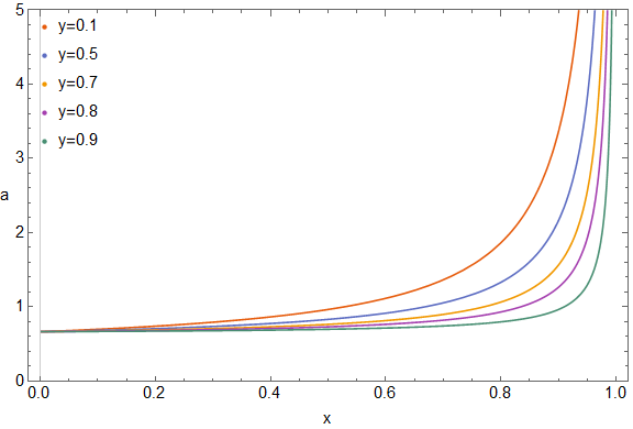
(a) $d=5$, $y$ fixed

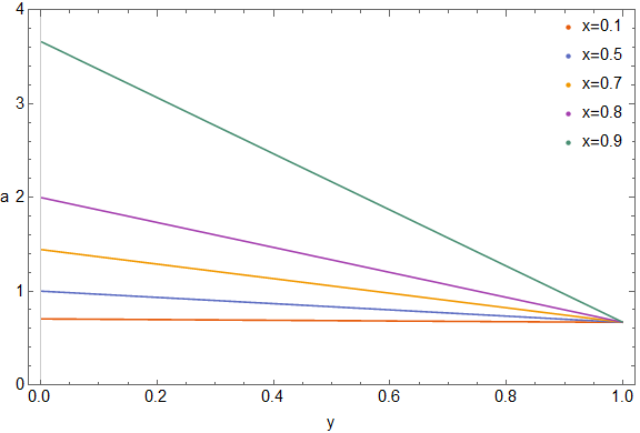
(b) $d=5$, $x$ fixed

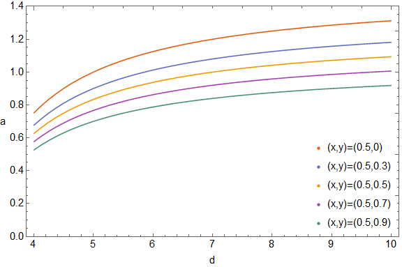
(c) $(x,y)$ fixed

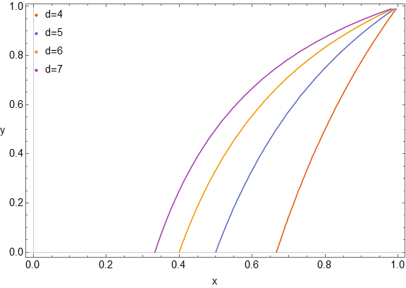
(d) $a=1$

Figure 5: Thermodynamic stability of the shell considering mass and charge fluctuations together is described, see Sec. IV.8 and Eqs. (75) and (76). Plots of $S_{5}\left(d,a,x,y\right)=0$, with $d$ being the number of spacetime dimensions, $a$ being the exponent of the equation of state of the shell, $x=\frac{r_{+}^{d-3}}{R^{d-3}}$, and $y=\frac{r_{-}^{d-3}}{r_{+}^{d-3}}$, where $r_{+}$ and $r_{-}$ are the gravitational radius and the Cauchy radius of the Reissner-Nordström shell spacetime, respectively, and $R$ is the radius of the shell, are shown. The equality $S_{5}\left(d,a,x,y\right)=0$ describes marginal stability of the shell considering together mass and charge fluctuations. (a) The function is plotted as $a(x)$ with $d=5$ and for fixed values of $y$, with points with lower $a$ than the function corresponding to stable configurations; (b) The function is plotted as $a(y)$ with $d=5$ and for fixed values of $x$, with points with lower $a$ corresponding to stable configurations; (c) The function is plotted as $a(d)$ for fixed values of the pair $(x,y)$, with points with lower $a$ corresponding to stable configurations; (d) The function is plotted as $y(x)$ for $a=1$ with fixed values of $d$, with configurations with higher $x$ than the curve being stable.

where Eqs. (64) and (65) have been used. The condition given in Eq. (76) is sufficient to describe the stability, since the right hand side of it is lower than the condition given by Eq. (68), in the respective parameter space. The inequality is quite simple enough for analytical treatment. The function set by the right-hand side at $x=0$ or $y=1$ takes the value $a=\frac{d-3}{d-2}$. At $x=1$, the function diverges to infinity. Thus, the function bends from a constant value to $a=\frac{d-3}{2(d-2)}\,\frac{2-x}{1-x}$, going from $y=1$ to $y=0$. A detailed analysis of Eq. (76) can be seen in Fig. 5 which is itself split into four plots (a), (b), (c), and (d). The case of the shell with thermodynamic black hole features, i.e., the case with $a=1$, shows that increasing the value of $y$ will decrease the range of $x$ for thermodynamic stable configurations, i.e., if the shell has more electric charge, then it must have lower radius $R$ for stability, see also Fig. 1(d) for this $a=1$ case.

IV.9 Area and charge fluctuations together

A shell with area and charge fluctuations will have the stability conditions given by $S_{AA}\leq 0$, $S_{QQ}\leq 0$, and $S_{AA}S_{QQ}-S_{AQ}^{2}\geq 0$, see Eq. (56). Note, however, that there is redundancy on this system of inequations, see Appendix B. The sufficient conditions can be chosen to be $S_{AA}\leq 0$ and $S_{AA}S_{QQ}-S_{AQ}^{2}\geq 0$. For the equations of state we are using, one has that $S_{AA}\leq 0$ yields Eq. (70), and with the help of Eq. (62) one has that $S_{AA}S_{QQ}-S_{AQ}^{2}\geq 0$ can be written as

$$S_{6}=-\frac{(1-x)}{2(d-3)}S_{2}S_{3}+xyS_{23}\leq 0\,.$$ (77)

Then, from Eq. (LABEL:eq:Sfunctions) this inequality can be rearranged as

$$a\leq\frac{\frac{(1-x)\mathcal{F}(2d-5)}{2(d-3)}(1+3y)-x^{3}y(1-y)+2\mathcal{F}xy-\frac{y\mathcal{F}^{2}}{x(1-y)}}{(d-2)(1-x)\Big{(}\frac{\mathcal{F}^{2}}{2x(d-3)}+\frac{2d-5}{(d-3)^{2}}y(1-x)\mathcal{F}+\frac{2\mathcal{F}xy}{(d-3)}\Big{)}}$$

$$+\frac{(d-3)}{(d-2)}\,\frac{1+y}{1-y}\,.$$ (78)

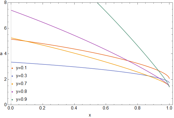
(a) $d=5$, $y$ fixed

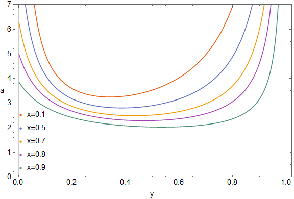
(b) $d=5$, $x$ fixed

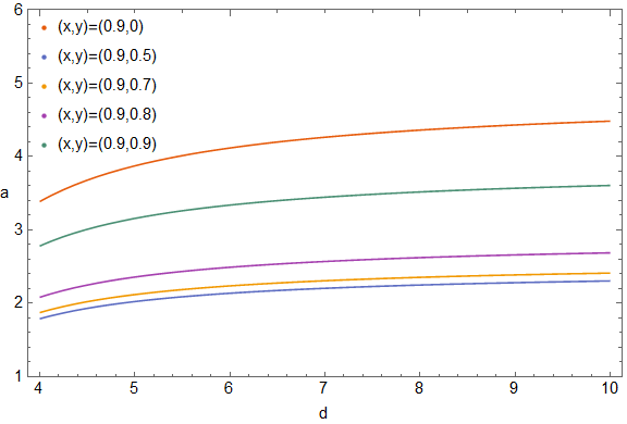
(c) $(x,y)$ fixed

Figure 6: Thermodynamic stability of the shell considering area and charge fluctuations together is described, see Sec. IV.9 and Eqs. (77) and (78). Plots of $S_{6}\left(d,a,x,y\right)=0$, with $d$ being the number of spacetime dimensions, $a$ being the exponent of the equation of state of the shell, $x=\frac{r_{+}^{d-3}}{R^{d-3}}$, and $y=\frac{r_{-}^{d-3}}{r_{+}^{d-3}}$, where $r_{+}$ and $r_{-}$ are the gravitational radius and the Cauchy radius of the Reissner-Nordström shell spacetime, respectively, and $R$ is the radius of the shell, are shown. The equality $S_{6}\left(d,a,x,y\right)=0$ describes marginal stability of the shell considering together area and charge fluctuations. (a) The function is plotted as $a(x)$ with $d=5$ and for fixed values of $y$; (b) The function is plotted as $a(y)$ with $d=5$ and for fixed values of $x$; (c) The function is plotted as $a(d)$ for fixed values of the pair $(x,y)$. Points with lower $a$ than the given function correspond to stable configurations in all three plots. All the configurations with $a=1$ are below the surface of marginal stability, therefore they are stable and there is no need for a plot (d).

where Eqs. (64) and (65) have been used. The condition given in Eq. (78) is sufficient to describe the stability, since the right hand side of it is lower than the condition given by Eq. (70), in the respective parameter space. At $y=0$, the function set by the right-hand side intersects $S_{2}$. The function then grows without bound at $(x=0,y=0)$ or $y=1$. In the limit of $x\rightarrow 1$, the function approaches the value of $a=\frac{8+6y-3d(1+y)}{(d-2)(1+3y)}$. At $x=0$, the right-hand side approaches $S_{3}$ from below. A detailed analysis of Eq. (78) can be seen in Fig. 6 which is itself split into three plots (a), (b), and (c). The case of the shell with thermodynamic black hole features, i.e., the case with $a=1$, does not need a more detailed analysis since all the configurations with $a=1$ are below the surface of marginal stability, therefore they are stable to these thermodynamic perturbations.

IV.10 Mass, area, and charge fluctuations altogether

A shell with mass, area, and charge fluctuations will have the stability conditions given by all the inequalities in Eq. (56). Note, however, that there is redundancy on this system of inequations, see Appendix B. The sufficient conditions can be chosen to be $S_{MM}\leq 0$, $S_{MM}S_{AA}-S_{MA}^{2}\geq 0$, and $(S_{MM}S_{AQ}-S_{MA}S_{MQ})^{2}-(S_{AA}S_{MM}-S_{AM}^{2})(S_{QQ}S_{MM}-S_{QM}^{2})\leq 0$. For the equations of state we are using, one has that $S_{MM}\leq 0$ yields Eq. (68), $S_{MM}S_{AA}-S_{MA}^{2}\geq 0$ yields Eq. (74), and with the help of Eq. (62) one has that $(S_{MM}S_{AQ}-S_{MA}S_{MQ})^{2}-(S_{AA}S_{MM}-S_{AM}^{2})(S_{QQ}S_{MM}-S_{QM}^{2})\leq 0$ can be written as

$$S_{7}=\left(xS_{1}S_{23}-\frac{2k}{d-3}S_{12}S_{13}\right)^{2}y-S_{4}S_{5}\leq 0\,.$$ (79)

Then, even though Eq. (79) appears to be a polynomial on $a$ of degree 4, from Eq. (LABEL:eq:Sfunctions) this inequality can be rearranged as

$$a\leq\frac{d-3}{d-2}\left(\frac{4-4k+x^{2}(d(1-y)^{2}+C)}{4-4k+x^{2}d(1-y)^{2}+xD}\right)\,,$$ (80)

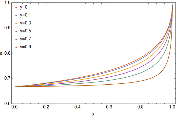
(a) $d=5$, $y$ fixed

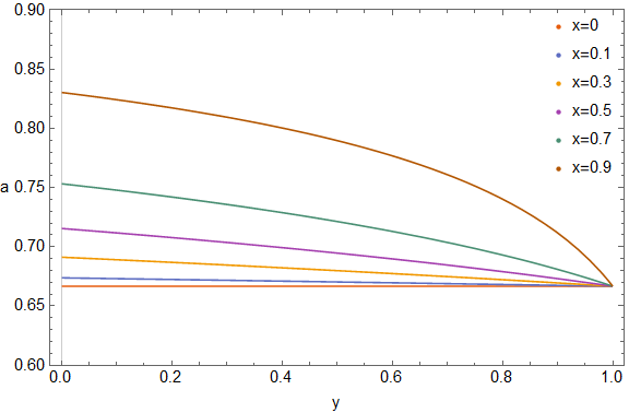
(b) $d=5$, $x$ fixed

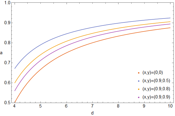
(c) $(x,y)$ fixed

Figure 7: Thermodynamic stability of the shell considering mass, area, and charge fluctuations altogether is described, see Sec. IV.10 and Eqs. (79) and (80). Plots of $S_{7}\left(d,a,x,y\right)=0$, with $d$ being the number of spacetime dimensions, $a$ being the exponent of the equation of state of the shell, $x=\frac{r_{+}^{d-3}}{R^{d-3}}$, and $y=\frac{r_{-}^{d-3}}{r_{+}^{d-3}}$, where $r_{+}$ and $r_{-}$ are the gravitational radius and the Cauchy radius of the Reissner-Nordström shell spacetime, respectively, and $R$ is the radius of the shell, are shown. The equality $S_{7}\left(d,a,x,y\right)=0$ describes marginal stability of the shell considering mass, area, and charge fluctuations altogether. (a) The function is plotted as $a(x)$ with $d=5$ and for fixed values of $y$; (b) The function is plotted as $a(y)$ with $d=5$ and for fixed values of $x$; (c) The function is plotted as $a(d)$ for fixed values of the pair $(x,y)$. Points with lower $a$ than the given function correspond to stable configurations in all three plots. All the configurations with $a=1$ are above the surface of marginal stability, hence they are unstable, except for the points with $x=1$ which lie on the limit of the surface, hence they are marginally stable, therefore they are stable and there is no need for a plot (d).

where $C=2x(1+y)(k-2)-2-2(y-4)y$, and $D=4k-2y-6-x\left(1+y(3y-8)\right)$, and Eqs. (64) and (65) have been used. The right-hand side of Eq. (80) when compared with the conditions in Eqs. (68) and (74) assumes always lower values, in the respective parameter space, therefore Eq. (80) is the sufficient condition of stability. The equality in the condition given in Eq. (80) has its lowest value of $a=\frac{d-3}{d-2}$ at $x=0$, for every $y$. It then increases toward $x=1$, where the limit gives $a=1$. At the limit of $y=1$, the equality is given by the lowest value of $a=\frac{d-3}{d-2}$ for every $x$ except $x=1$ where the limit gives $a=1$. Thus, the condition for stability in Eq. (80) implies that every configuration with $a\leq\frac{d-3}{d-2}$ is stable. On the other hand, for $\frac{d-3}{d-2}<a<1$ the stability region decreases with increasing $y$, being zero in the limit of $y=1$. This means that shells with more electric charge will have less configurations of stability. The space of stable configurations in the $a-d$ plane can also be made and is similar to the analysis made for the uncharged case in Andre:2019 . A detailed analysis of Eq. (80) can be seen in Fig. 7 which is itself split into three plots (a), (b), and (c). The case of the shell with thermodynamic black hole features, i.e., the case with $a=1$, does not need a more detailed analysis since all the configurations with $a=1$ are above the surface of marginal stability, hence unstable, except for the points with $x=1$ which lie on the limit of the surface, hence marginally stable. In the black hole limit, i.e., not only $a=1$ but also $x=1$, the configurations for every value of $y$ are marginally stable.

IV.11 Further comments on the behavior of intrinsic stability with $a$

We now make some important comments, leftovers from the previous sections.

When discussing mass fluctuations only, Sec. IV.4, we mentioned that one can make a corresponding stability analysis in terms of the variables $\frac{M}{R^{d-3}}$ and $\frac{Q}{R^{d-3}}$, instead of $x=\frac{r_{+}^{d-3}}{R^{d-3}}$ and $y=\frac{r_{-}^{d-3}}{r_{+}^{d-3}}$ of Eq. (65). The analysis in $\frac{M}{R^{d-3}}$ and $\frac{Q}{R^{d-3}}$ yields some interesting insight. The condition given in Eq. (68) becomes

$$a\leq\frac{\mu}{2}\frac{(d-3)}{(d-2)}\frac{\left(\frac{Q^{2}}{R^{2(d-3)}}+\frac{\mu M^{2}}{R^{2(d-3)}}-\frac{2M}{R^{d-3}}\right)}{\left(1-\frac{\mu M}{R^{d-3}}\right)^{2}}$$

$$\times\frac{\left(\frac{2\mu M}{R^{d-3}}+\frac{\mu(Q^{2}-M^{2}\mu^{2})}{R^{2(d-3)}}-2\right)}{\sqrt{\frac{\mu(\mu M^{2}-Q^{2})}{R^{2(d-3)}}\left(\left(2-\frac{\mu M}{R^{d-3}}\right)^{2}-\frac{\mu Q^{2}}{R^{2(d-3)}}\right)}}\,.$$ (81)

The possible physical values of $\frac{M}{R^{d-3}}$ and $\frac{Q}{R^{d-3}}$ are restricted by the condition of subextremality, i.e., $\sqrt{\mu}M>Q$, and the condition of no trapped surfaces, i.e., $\frac{r_{+}}{R}<1$. One finds from Eq. (81) that for small values of $\frac{M}{R^{d-3}}$, the shell needs some minimum charge $Q$, or correspondingly a minimum value of $\frac{Q}{R^{d-3}}$, for it to be stable. When $\frac{M}{R^{d-3}}$ has a value that corresponds to $x=\frac{2}{d-1}$, the minimum charge for the shell to be stable reaches zero, which means $y=0$. For higher $\frac{M}{R^{d-3}}$, the region of stability is restricted by the physically possible values, namely, $\frac{\sqrt{\mu}M}{R^{d-3}}>\frac{Q}{R^{d-3}}$ and $\frac{r_{+}}{R}<1$. Thus, in brief, for $\frac{M}{R^{d-3}}$ small, thermodynamic stability exists only for sufficiently large electric charge. For $\frac{M}{R^{d-3}}$ having a value such that $x=\frac{2}{d-1}$ when $y=0$, i.e., $Q=0$, the shell is marginally stable. Here, it is important to note that the value of $x=\frac{2}{d-1}$ for $Q=0$ means that the shell is at the photonic orbit . For higher values of $x$, maintaining $Q=0$, the shell is inside the photonic orbit, and it is stable. This means that for $\frac{M}{R^{d-3}}$ yielding values higher than $x=\frac{2}{d-1}$ when $y=0$, i.e, $Q=0$, the shell is thermodynamically stable, see also Andre:2019 . This latter behavior, i.e., the behavior for $\frac{M}{R^{d-3}}$ yielding values of $x$ equal or higher than $x=\frac{2}{d-1}$, is precisely the same behavior of the large black hole in the canonical ensemble found by York York:1986 ; can and generalized to $d$ dimensions in andrelemos1 ; andrelemos2 . For higher values of $\frac{M}{R^{d-3}}$ increasing the electrically charge $Q$, and so essentially increasing $\frac{Q}{R^{d-3}}$, does not alter the stability, the solutions are all thermodynamically stable. The result can be interpreted heuristically. To understand it, note that the reduced inverse temperature $b$, can be envisaged as a length scale, a thermal one. The inverse temperature $b$ here is the one given in Eq. (49). For small $\frac{M}{R^{d-3}}$ and $Q=0$ one has that the shells have radii higher than the photonic orbit and are thermodynamically unstable. What happens is that the thermal length $b$ being proportional to $M$, still in the uncharged case, is smaller than or of the order of the radius of the shell, and thus the shell loses energy and mass along these thermal lengths. Losing mass, means that the thermal length $b$ decreases, and so the process is a runaway process and thus unstable. If the charge $Q$ increases, or more correctly if the ratio $\frac{Q}{R^{d-3}}$ increases, the thermal length $b$ gets correspondingly higher, and for a certain sufficiently high electric charge $Q$, or better for a sufficiently high $\frac{Q}{R^{d-3}}$, $b$ is now sufficiently greater than the radius of the shell, so that it is not possible to lose energy anymore. Thus, the electric shell is stable for charges higher than this minimum electric charge. For higher electric charge, i.e., higher $\frac{Q}{R^{d-3}}$, such that one is near the extremal limit, one has that $b$ is proportional to $\frac{1}{\sqrt{M-Q}}$ and so it is indeed divergingly larger than $R$. For $Q=0$ and a value of $\frac{M}{R^{d-3}}$ such that $x=\frac{2}{d-1}$, one has a shell with radius equal to the photonic orbit. In this case the thermal length $b$, as the calculations show, is barely sufficiently to not allow thermal loss from the shell, and so maintain the shell in thermodynamic equilibrium. For higher $\frac{M}{R^{d-3}}$ and $Q=0$, the shell is inside the photonic orbit, and the thermal length $b$ is now sufficiently large relatively to the radius of the shell to not allow thermal loss from the shell, and this holds even truer for higher $Q$, i.e., higher $\frac{Q}{R^{d-3}}$, where $b$ gets even larger and thus the shell in all these cases is thermodynamically stable. The comments made here for generic dimensions $d$, apply to the $d=4$ electric charged case studied in Lemos:2015a and are exemplified for $d=5$ in Fig. 1(d) bottom.

Another important point, is that in Sec. IV.10 we have pointed out that for mass, area, and charge fluctuations altogether, shells with more electric charge will have less configurations of stability. This behavior differs from the case of mass fluctuations only of Sec. IV.4 that was also commented in the previous paragraph, where, for certain configurations, more electric charge aids to the stability. There is no contradiction between the two cases. The mass, area, and charge fluctuations altogether is much more restrictive than the mass fluctuations only case, in the sense that stable points in the former fluctuations are also stable points in the latter fluctuations, but the converse is not true.

There is still another point worth noting. In the case of one or two fixed quantities, Secs. IV.4-IV.9, there are shell configurations with $a\geq 1$ that are stable. But one notices that the higher the $a$ the higher the entropy $S$ since it goes with a power of $a$. For instance, for the area fluctuations only of Sec. IV.5, we have seen that Eq. (70) has its minimum at $\frac{r_{+}}{R}=1$ for zero charge, i.e., $(x=1,y=0)$, with the value for $a$ given by $a=3-\frac{2}{d-2}$. Since values of $a=3-\frac{2}{d-2}$ are always greater than one, this could mean that a shell with lower $a$ would tend to settle into a shell with higher $a$ since the latter would have higher entropy. One could think that a change of $a$ could be achieved by some rearrangement of the material on the shells and in this way higher entropies could be attained. However, the stability analysis performed is for fixed $a$, since the very exponent $a$ gives a precise temperature equation of state for the matter, and to treat changes in the exponent $a$ one would have perhaps to envisage some type of phase transition.

Having worked out the thermodynamic stability criterion for all types of fluctuation in Secs. IV.4-IV.10 through the parameter $a$, it begs now the question of what is the physical reason for the behavior of the intrinsic stability with $a$ itself. We now turn into this point.

V Intrinsic thermodynamic stability in laboratory variables

V.1 The rational to introduce laboratory variables

It begs now the question of what is the physical reason for the behavior of intrinsic stability with $a$. In order to understand the physical meaning of the intrinsic thermodynamic stability associated to this self-gravitating thin shell, we rewrite the stability conditions with variables that can be measured in the laboratory. One of these variables that we are going to define gives a good example of the way the stability conditions get clearer when written in terms of thermodynamic coefficients. The heat capacity at constant area and charge, $C_{A,Q}$, can be defined as $C_{A,Q}^{-1}=\left(\frac{\partial T}{\partial M}\right)$. This variable is important since we also have $S_{MM}=-\beta^{2}C_{A,Q}^{-1}\leq 0$, and so the stability condition for changes in proper mass only is that the heat capacity $C_{A,Q}$ is positive. The aim is to generalize this reasoning for two types of fluctuations which seem the most interesting, namely, the mass and charge fluctuations studied in Sec. IV.8, and mass, area, and charge fluctuations studied in Sec. IV.10.

V.2 Laboratory variables for mass and charge fluctuations together

Here we discuss the new laboratory variables for mass and charge fluctuations, see Sec. IV.8. It emerges that the heat capacities at fixed area play an important role when treating mass and charge fluctuations together. There are two such heat capacities, namely, the heat capacity at constant area and electric charge $C_{A,Q}$, and the heat capacity at constant area and electric potential $C_{A,\Phi}$.

The three equations of state $T(M,A,Q)$, $p(M,A,Q)$, and $\Phi(M,A,Q)$, given in Eqs. (58)-(60) are to be rewritten in laboratory variables, which are also called thermodynamic coefficients. In fact, for mass and charge fluctuations, one only needs two equations of state, the ones for the temperature $T(M,A,Q)$ and for the thermodynamic electric potential $\Phi(M,A,Q)$. Since the area is kept fixed here we do not need to use the equation of state for the pressure, $p(M,A,Q)$. The equations for $T(M,A,Q)$ and $\Phi(M,A,Q)$ will allow us to establish the stability conditions for mass and charge fluctuations in the new variables.

For the equation of state for temperature, $T(M,A,Q)$, we want to define the laboratory variables in terms of the derivatives of $S(T,A,Q)$. For that, note that one is able to write the differential $dS(T,A,Q)$ as $dS=\left(\frac{\partial S}{\partial T}\right)_{A,Q}dT+\left(\frac{\partial S}{\partial A}\right)_{T,Q}dA+\left(\frac{\partial S}{\partial Q}\right)_{T,A}dQ$. Now, the heat capacity $C_{A,Q}$ is defined as $C_{A,Q}^{-1}=\left(\frac{\partial T}{\partial M}\right)_{A,Q}$ which is equivalent to $\frac{1}{T}C_{A,Q}=\left(\frac{\partial S}{\partial T}\right)_{A,Q}$. The latent heat capacity at constant temperature and charge, $\lambda_{T,Q}$, is defined as $\lambda_{T,Q}=\left(\frac{\partial S}{\partial A}\right)_{T,Q}$. The latent heat capacity at constant temperature and area, $\lambda_{T,A}$, is defined as $\lambda_{T,A}=\left(\frac{\partial S}{\partial Q}\right)_{T,A}$. One can then change the equality for $dS$ into an equality for $dT$, such that $T=T(S,A,Q)$, to obtain $dT=\frac{T}{C_{A,Q}}dS-T\frac{\lambda_{T,Q}}{C_{A,Q}}dA-\frac{T\lambda_{T,A}}{C_{A,Q}}dQ$. One can now use the first law, Eq. (36), i.e., $TdS=dM+pdA-\Phi dQ$, substitute for the variation of the entropy $dS$ above and put the equation found as an equality for $dT$, namely,

$$dT=\frac{1}{C_{A,Q}}dM-\frac{T\lambda_{T,Q}-p}{C_{A,Q}}dA-\frac{T\lambda_{T,A}+\Phi}{C_{A,Q}}dQ\,,$$ (82)

So, $dT$ is written in terms of the laboratory variables, namely, the heat capacity $C_{A,Q}$, the latent heat capacity at constant temperature and charge $\lambda_{T,Q}$, and the latent heat capacity at constant temperature and area $\lambda_{T,A}$. For the equation of state for the thermodynamic electric potential $\Phi(M,A,Q)$, we define the laboratory variables with respect to $\Phi(S,A,Q)$ so that, with the aid of $S(M,A,Q)$, we obtain $\Phi(M,A,Q)$. Now, note that one is able to write the differential $d\Phi(S,A,Q)$ as $d\Phi=\left(\frac{\partial\Phi}{\partial S}\right)_{A,Q}dS+\left(\frac{\partial\Phi}{\partial A}\right)_{S,Q}dA+\left(\frac{\partial\Phi}{\partial Q}\right)_{S,A}dQ$. We define the adiabatic electric susceptibility, $\chi_{S,A}$, as $\frac{1}{\chi_{S,A}}=\left(\frac{\partial\Phi}{\partial Q}\right)_{S,A}$, and define the electric pressure at constant entropy and charge, $P_{S,Q}$, as $P_{S,Q}=\left(\frac{\partial\Phi}{\partial A}\right)_{S,Q}$. The remaining derivative of $\Phi$ is given by the Maxwell relation $\left(\frac{\partial\Phi}{\partial S}\right)_{A,Q}=\left(\frac{\partial T}{\partial Q}\right)_{S,A}=-\frac{T\lambda_{T,A}}{C_{A,Q}}$, which was calculated using the definitions given above for $C_{A,Q}$, $\lambda_{T,Q}$, and $\lambda_{T,A}$, and swapping the equality for $dS(T,A,Q)$ into an equality for $d\Phi(S,A,Q)$, i.e., $d\Phi=-\frac{T\lambda_{T,A}}{C_{A,Q}}dS+P_{S,Q}dA+\frac{1}{\chi_{S,A}}dQ$. One can now use the first law, Eq. (36), i.e., $TdS=dM+pdA-\Phi dQ$, substitute for the variation of the entropy $dS$ above and the equation found as an equality for $d\Phi$, namely,

$$d\Phi=-\frac{\lambda_{T,A}}{C_{A,Q}}dM+\left(P_{S,Q}-p\frac{\lambda_{T,A}}{C_{A,Q}}\right)dA$$

$$+\left(\frac{1}{\chi_{S,A}}+\frac{\Phi\lambda_{T,A}}{C_{A,Q}}\right)dQ\,.$$ (83)

So, $d\Phi$ is written in terms of the laboratory variables, namely, the heat capacity, $C_{A,Q}$, the latent heat capacity at constant temperature and area, $\lambda_{T,A}$, the electric pressure at constant entropy and charge, $P_{S,Q}$, and the adiabatic electric susceptibility, $\chi_{S,A}$. Finally, it is useful to define also the heat capacity at constant area and constant electric potential, $C_{A,\Phi}$, defined by $C_{A,\Phi}=T\left(\frac{\partial S}{\partial T}\right)_{A,\Phi}$ which can be written in terms of the coefficients in Eqs. (82) and (83) as $C_{A,\Phi}=C_{A,Q}\left(1-\frac{T\lambda_{T,A}^{2}}{C_{A,Q}}\chi_{S,A}\right)^{\hskip-4.26773pt-1}$.

The intrinsic thermodynamic stability of a thin shell for mass and charge fluctuations together can be determined by considering the two sufficient stability conditions which can be taken from Eq. (56), yielding $S_{MM}\leq 0$ and $S_{MM}S_{QQ}-S_{MQ}^{2}\geq 0$. The first condition is almost immediate since with the definition in Eq. (82) we obtain $S_{MM}=-\beta^{2}\frac{1}{C_{A,Q}}$ and so it implies that $C_{A,Q}\geq 0$. The second condition requires some more care and some more algebra, yielding in the end $S_{MM}S_{QQ}-S_{MQ}^{2}=\ \beta^{2}\frac{1}{C_{A,\Phi}\chi_{S,A}}$, and so it implies $C_{A,\Phi}\,\,\chi_{S,A}\geq 0$. The stability conditions in the laboratory variables can then be written as

$$C_{A,Q}\geq 0\,,$$

$$C_{A,\Phi}\,\,\chi_{S,A}\geq 0\,.$$ (84)

For the specific equations of state we used, Eqs. (58)-(60), the coefficient $\chi_{S,A}$ is always positive. Hence, from the two equations given in Eq. (V.2) , the stability conditions become $C_{A,Q}\geq 0$ and $C_{A,\Phi}\geq 0$, respectively. Moreover, we have found in Sec. IV.8 that for these equations of state the condition $S_{MM}S_{QQ}-S_{MQ}^{2}\geq 0$ is the sufficient condition for stability. Therefore, the thin shell considered is thermodynamic stable for mass and charge fluctuations together if

$$C_{A,\Phi}\geq 0\,.$$ (85)

This occurs precisely when Eq. (76) is satisfied, i.e., Eq. (85) is equivalent to Eq. (76), as for a thin shell with the equations of state given in Eqs. (58)-(60). Note that, when there is equality in Eq. (76), one must be careful in regard to the value of the heat capacity at constant area and constant electric potential, $C_{A,\Phi}$. If one performs the limit to the equality as a succession of stable configurations, by starting from a configuration with the exponent $a$ satisfying Eq. (85) and then increasing $a$, the coefficient $C_{A,\Phi}$ becomes infinite and positive. If, on the contrary, one performs the limit to the equality as a succession of unstable configurations, by starting from a configuration with the exponent $a$ not satisfying Eq. (85) and then decreasing $a$, the coefficient $C_{A,\Phi}$ becomes infinite and negative.

The details of all the calculations presented in this section are shown in Appendix D.1.

V.3 Laboratory variables for mass, area, and charge fluctuations altogether

Here we discuss the new laboratory variables for mass, area, and charge fluctuations, see Sec. IV.10. The analysis in Sec. V.2 highlights the importance of the specific heat capacities $C_{A,Q}$ and $C_{A,\Phi}$ in the intrinsic stability of thermodynamic systems with fixed area. Nevertheless, there are other important quantities playing a role in the intrinsic stability for the case of mass, area and charge fluctuations. In this case the important laboratory quantities are the heat capacity at constant area and electric charge $C_{A,Q}$ again, the expansion coefficient at constant temperature and electric charge $\kappa_{T,Q}$, and the electric susceptibility at constant pressure and temperature $\chi_{p,T}$.

The three equations of state $T(M,A,Q)$, $p(M,A,Q)$, and $\Phi(M,A,Q)$ are to be rewritten in laboratory variables. This will allow us to establish the stability conditions in these new variables for mass, area, and charge fluctuations, and so no fixed quantities. We now want to define the laboratory variables in terms of the derivatives of $S(T,p,Q)$, $A(T,p,Q)$, and $\Phi(T,p,Q)$, for convenience, since these variables will simplify the considered stability conditions. Notice that the three functions $S(T,p,Q)$, $A(T,p,Q)$ and $\Phi(T,p,Q)$ are the derivatives of the Gibbs potential, i.e., $dG=-SdT+Adp+\Phi dQ$. Let us start with the area $dA$ for which the coefficients have a direct physical meaning. We write $dA=\left(\frac{\partial A}{\partial T}\right)_{p,Q}dT+\left(\frac{\partial A}{\partial p}\right)_{T,Q}dp+\left(\frac{\partial A}{\partial Q}\right)_{T,p}dQ$, such that $\alpha_{p,Q}=\frac{1}{A}\left(\frac{\partial A}{\partial T}\right)_{p,Q}$ is the expansion coefficient, $\kappa_{T,Q}=-\frac{1}{A}\left(\frac{\partial A}{\partial p}\right)_{T,Q}$ is the isothermal compressibility, and $\kappa_{p,T}=-\frac{1}{A}\left(\frac{\partial A}{\partial Q}\right)_{T,p}$ is the electric compressibility. Now, $dS$ is written as $dS=\left(\frac{\partial S}{\partial T}\right)_{p,Q}dT+\left(\frac{\partial S}{\partial p}\right)_{T,Q}dp+\left(\frac{\partial S}{\partial Q}\right)_{T,p}dQ$, where $\left(\frac{\partial S}{\partial T}\right)_{p,Q}$ can be written in terms of previously defined coefficients, specifically, $\left(\frac{\partial S}{\partial T}\right)_{p,Q}=\frac{C_{A,Q}}{T}+A\frac{\alpha_{p,Q}^{2}}{\kappa_{T,Q}}$, $\left(\frac{\partial S}{\partial p}\right)_{T,Q}$ can be written using the Maxwell relation $\left(\frac{\partial S}{\partial p}\right)_{T,Q}=-\left(\frac{\partial A}{\partial T}\right)_{T,Q}=A\alpha_{p,Q}$, and $\lambda_{p,T}=\left(\frac{\partial S}{\partial Q}\right)_{p,T}$ is a new coefficient, the latent heat capacity. Finally, $d\Phi$ is written as $d\Phi=\left(\frac{\partial\Phi}{\partial T}\right)_{p,Q}dT+\left(\frac{\partial\Phi}{\partial p}\right)_{T,Q}dp+\left(\frac{\partial\Phi}{\partial Q}\right)_{T,p}dQ$, where two of the derivatives are written using Maxwell relations, i.e., $\left(\frac{\partial\Phi}{\partial T}\right)_{p,Q}=-\left(\frac{\partial S}{\partial Q}\right)_{p,T}=\lambda_{p,T}$ and $\left(\frac{\partial\Phi}{\partial p}\right)_{T,Q}=\left(\frac{\partial A}{\partial Q}\right)_{p,T}=-A\kappa_{p,T}$ as defined above, and $\frac{1}{\chi_{p,T}}=\left(\frac{\partial\Phi}{\partial Q}\right)_{p,T}$ is a new coefficient, the isothermal electric susceptibility. With the differentials $dA(T,p,Q)$, $dS(T,p,Q)$ defined above in terms of physical coefficients, we are able to invert the system composed by these two differentials in order to obtain $dT(S,A,Q)$ and $dp(S,A,Q)$. Then, using Eq. (36), i.e., $TdS=dM+pdA-\Phi dQ$, we are able to obtain the differentials of the two equations of state in the desired form, i.e., $dT(M,A,Q)$ and $dp(M,A,Q)$. Inserting $dT(M,A,Q)$ and $dp(M,A,Q)$ into $d\Phi(T,p,Q)$, we find the differential of the remaining equation of state, $d\Phi(M,A,Q)$. Thus, these differentials are written in terms of the defined laboratory variables and the differentials of $dM$, $dA$, and $dQ$, as

$$dT= \frac{dM}{C_{A,Q}}+\left(\frac{p}{C_{A,Q}}-T\frac{\alpha_{p,Q}}{C_{A,Q}\kappa_{T,Q}}\right)dA$$

$$-\left(\frac{\Phi}{C_{A,Q}}+T\frac{\lambda_{p,T}}{C_{A,Q}}+A\frac{\alpha_{p,T}\kappa_{p,T}}{\kappa_{T,Q}C_{A,Q}}\right)dQ\,,$$ (86)

$$dp= \frac{\alpha_{p,Q}}{C_{A,Q}\kappa_{T,Q}}dM$$

$$-\left[\frac{1}{A\kappa_{T,Q}}-\frac{\alpha_{p,Q}}{C_{A,Q}\kappa_{T,Q}}\left(p-T\frac{\alpha_{p,Q}}{\kappa_{T,Q}}\right)\right]dA$$

$$-\left(\frac{\kappa_{p,T}}{\kappa_{T,Q}}-\frac{\alpha_{p,Q}}{C_{A,Q}\kappa_{T,Q}}\mathcal{C}\right)dQ\,,$$ (87)

$$d\Phi= -\mathcal{B}dM+\left[\frac{\kappa_{p,T}}{\kappa_{T,Q}}-\left(p-T\frac{\alpha_{p,Q}}{\kappa_{T,Q}}\right)\mathcal{B}\right]dA$$

$$+\left(\mathcal{B}\mathcal{C}+\frac{1}{\chi_{p,T}}+A\frac{\kappa_{p,T}^{2}}{\kappa_{T,Q}}\right)dQ\,,$$ (88)

where $\mathcal{B}$ is defined as $\mathcal{B}=A\frac{\kappa_{p,T}\alpha_{p,Q}}{C_{A,Q}\kappa_{T,Q}}+\frac{\lambda_{p,T}}{C_{A,Q}}$, and $\mathcal{C}$ is defined as $\mathcal{C}=TA\frac{\kappa_{p,T}\alpha_{p,Q}}{\kappa_{T,Q}}+T\lambda_{p,T}+\Phi$. With the differentials $dT(M,A,Q)$, $dp(M,A,Q)$, and $d\Phi(M,A,Q)$ in Eqs. (86)-(88), and the first law of thermodynamics, Eq. (36), i.e., $TdS=dM+pdA-\Phi dQ$, the second derivatives of the entropy that enter into the thermodynamic stability problem and are given in Eq. (62) can be calculated directly.

The intrinsic thermodynamic stability of a thin shell for generic mass, area, and charge fluctuations, is given by the three sufficient stability conditions which can be taken from Eq. (56), yielding $S_{MM}\leq 0$, $S_{MM}S_{AA}-S_{MA}^{2}\geq 0$, and $(S_{MM}S_{AQ}-S_{MA}S_{MQ})^{2}-(S_{AA}S_{MM}-S_{AM}^{2})(S_{QQ}S_{MM}-S_{QM}^{2})\leq 0$. Now, having the second derivatives of the entropy written in terms of the laboratory variables defined in this section, one finds that $S_{MM}\leq 0$ is equivalent to $\beta^{2}\frac{1}{C_{A,Q}}\geq 0$, $S_{MM}S_{AA}-S_{MA}^{2}\geq 0$ is equivalent to $\beta^{3}\frac{1}{A\kappa_{T,Q}C_{A,Q}}\geq 0$, and $(S_{MM}S_{AQ}-S_{MA}S_{MQ})^{2}-(S_{AA}S_{MM}-S_{AM}^{2})(S_{QQ}S_{MM}-S_{QM}^{2})\leq 0$ is equivalent to $\beta^{6}\frac{1}{AC_{A,Q}^{2}\kappa_{T,Q}\,\,\chi_{p,T}}\geq 0$. We then have that the stability conditions for generic mass, area, and charge fluctuations are given by the following three equations,

$$C_{A,Q}\geq 0,\,$$

$$\kappa_{T,Q}\geq 0\,,$$

$$\chi_{p,T}\geq 0\,,$$ (89)

i.e., all three laboratory quantities have to be positive, specifically, the heat capacity $C_{A,Q}$ which is related to changes in temperature, the isothermal compressibility $\kappa_{T,Q}$ which is related to changes in the pressure, and the isothermal electric susceptibility $\chi_{p,T}$ which is related to changes in the electric charge, have to be positive, with the case of marginal stability corresponding to these physical variables going to infinity.

For the specific equations of state we use, Eqs. (58)-(60), for $T$, $p$, and $\Phi$, respectively, one finds that the most restrictive condition is for $\chi_{p,T}$,

$$\chi_{p,T}\geq 0\,,$$ (90)

so the positivity of the isothermal electric susceptibility $\chi_{p,T}$ is the sufficient condition in the case of the thin shell we are considering, with marginal stability happening when this quantity is infinite, and with the unstable configurations having a negative electric susceptibility and thus departing from equilibrium. Making the connection to Sec. IV.10, Eq. (90) is equivalent to Eq. (80) and one finds that for $a<\frac{d-3}{d-2}$ the isothermal electric susceptibility $\chi_{p,T}$ will always be positive, for $\frac{d-3}{d-2}<a<1$ it will be positive for some values of $(r_{+},r_{-},R)$, for $a=1$ and $R>r_{+}$ it will be negative with the case $R=r_{+}$ having to be treated with care, and for $a>1$ it will always be negative. The shell with black hole features, namely, $a=1$ and $R=r_{+}$, is thermodynamic unstable if the shell approaches its own gravitational radius $r_{+}$, $R\to r_{+}$, since in this case $\chi_{p,T}\rightarrow-\infty$. But there is the possibility, of having a configuration with $R=r_{+}$ that is created from the start, i.e., a configuration not belonging to a sequence of quasistatic configurations that has its radius $R$ decreased up to $r_{+}$. In this case the stability depends on whether the exponent $a$ of the equation of state approaches $a=1$ from below or from above. If the exponent $a$ of the equation of state approaches $a=1$ from below then the $R=r_{+}$ configuration is marginally stable with $\chi_{p,T}\rightarrow+\infty$, which means that changes in the electric charge of the configuration will not have any impact on the electric potential. If the exponent $a$ of the equation of state approaches $a=1$ from above then the $R=r_{+}$ configuration is unstable, $\chi_{p,T}\rightarrow-\infty$. Moreover, in the region of $\frac{d-3}{d-2}<a<1$, shells with more electric charge show more difficulty in having positive isothermal electric susceptibility $\chi_{p,T}$, a property that can be deduced from Fig. 7 by the decreasing amount of stable configurations with electric charge.

The details of all the calculations presented in this section are shown in Appendix D.2.

VI Conclusions

We have used the thin shell formalism to determine the mechanics of a static charged spherical thin shell in $d$ dimensions in general relativity and studied its thermodynamics by imposing the first law. The fact that the rest mass density and so the rest mass behaves as a thermal quasilocal energy and that the pressure is determined just by general relativity indicates there is a relation between general relativity and thermodynamics as one equation of state of the shell becomes fixed. We computed the entropy in terms of the thermodynamic quantities of the shell, namely, the rest mass $M$, the area $A$ and the electric charge $Q$ of the shell. The derivatives of the entropy are directly related to the temperature and the electric potential. Indeed, with the first law of thermodynamics and general relativity alone, we were able to restrict the expressions for the equations of state for the temperature and the thermodynamic electric potential. These equations of state in turn imply that the entropy $S$ depends solely on the two natural radius of the Reissner-Nordström shell spacetime, the gravitational radius $r_{+}$ and the Cauchy radius $r_{-}$, which in turn depend on $M$, $A$ and $Q$. That the entropy $S$ of the $d$ dimensional shell spacetime does not depend on the radius of the shell, $R$, is a remarkable fact, which nevertheless has been found for other thin shell spacetimes.

To calculate an exact expression for the entropy of the shell, one still needs full expressions for the temperature and the thermodynamic electric potential equations of state. We used a power law in $r_{+}$ with exponent $a$ for the temperature, and opted for the characteristic electric potential of a Reissner-Nordström shell spacetime, to obtain that the entropy $S$ of the shell is proportional to $A_{+}^{a}$, where $A_{+}$ is the gravitational area corresponding to $r_{+}$. Shells with such entropy are of great interest as it is possible to obtain the black hole limit and recover the thermodynamics of black holes.

We have then studied the thermodynamic intrinsic stability of thin shells with such an entropy equation. The shell is stable if the Hessian of the entropy is negative semidefinite. We analyzed the Hessian for seven possible types of fluctuations that can occur in the shell. Fluctuations of the shell with one free and two fixed thermodynamic quantities are of three types, fluctuations of the shell with two free and one fixed quantities are also of three types, and fluctuations of the shell with three free quantities, i.e., no fixed quantities, are of one type. The most important and general type of fluctuations are the ones with no fixed quantities. In the case of our entropy equation, we have found that only one condition is sufficient for the shell to be stable. This condition establishes that for $0<a\leq\frac{d-3}{d-2}$ all the configurations of the shell are thermodynamic stable, for $\frac{d-3}{d-2}<a<1$ stability depends on the mass and electric charge, for $a=1$ the configurations are unstable, unless the shell is at its own gravitational radius, i.e., at the black hole limit, in which case it is marginally stable, and that for $1<a<\infty$ all configurations are unstable.

The physical interpretation for the stability is analyzed through new thermodynamic variables that can be measured in the laboratory. One finds that, generically, stable shells have positive heat capacity, positive isothermal compressibility, and positive isothermal electric susceptibility. For the specific equations of state that we gave, and so for our entropy equation, it is found that every shell with positive electric susceptibility has positive heat capacity and positive isothermal compressibility, which is an interesting property of the shells with the considered entropy. In addition, marginal stability means that the electric susceptibility is infinite, which seems to be the case in the black hole limit. Shells with negative electric susceptibility depart from the initial state and they should rearrange themselves until the susceptibility becomes positive or the shell breaks down.

This work has derived some thermodynamic properties for electrically charged spherical matter shells in higher dimensions and complements a set of works in the thermodynamics of thin shells. Still, more future work should be done in the investigation of the link between thermodynamics and general relativity, and hopefully contribute to the understanding of black hole physics and with it trying to grasp gravitation at the tiniest possible scales.

Appendix A Temperature as a power law in the ADM mass and corresponding thermodynamic electric potential as alternative to the equations of state of Sec. III

The reduced equations of state for the inverse temperature and thermodynamic electric potential given in Eqs. (49) and  (50) of Sec. III are a good choice for reduced equations of state as they yield naturally the black hole equations of state. But there are alternatives to these equations of state.

In $d=4$, an alternative was provided in Lemos:2015a , where the reduced inverse temperature was chosen to be $b(r_{+},r_{-})=2a(r_{+}+r_{-})^{\alpha}$, for some constant $a$ and exponent $\alpha$. Thus, $b$, which represents the inverse temperature at infinity, is given as a power law depending on the ADM mass, since in $d=4$, one has $r_{+}+r_{-}=2Gm$. The solution for the reduced thermodynamic electric potential $c(r_{+},r_{-})$ is then $c(r_{+},r_{-})=2\gamma\frac{(r_{+}r_{-})^{\delta}}{(r_{+}+r_{-})^{\alpha}}$ for some $\gamma$, $\delta$, and so is a power law in the charge $Q$ combined with a power law in $m$ Lemos:2015a . For this $d=4$ case, it is possible analytically to study its stability.

Motivated by this choice for a reduced equation of state for $d=4$, we consider for a reduced equation of state for the temperature in generic $d$ dimensions, the following expression

$$b(r_{+},r_{-})=a(r_{+}^{d-3}+r_{-}^{d-3})^{\alpha}\,,$$ (91)

where $a$ and $\alpha$ are arbitrary real numbers, and such a choice means that $b$ is indeed a power law in the $d$-dimensional ADM mass $m$. With the chosen reduced equation of state for the inverse temperature, the condition in Eq. (48) can be used to restrict the form of $c(r_{+},r_{-})$, which is given in this case by $\frac{\partial c}{\partial r_{-}}\frac{r_{-}}{d-3}-\frac{\partial c}{\partial r_{+}}\frac{r_{+}}{d-3}=\alpha c\frac{r_{+}^{d-3}-r_{-}^{d-3}}{r_{+}^{d-3}+r_{-}^{d-3}}$. The general solution for $c(r_{+},r_{-})$ is

$$c(r_{+},r_{-})=\frac{f(r_{+}r_{-})}{(r_{+}^{d-3}+r_{-}^{d-3})^{\alpha}}\,,$$ (92)

where $f(r_{+}r_{-})$ is an arbitrary function depending only on the charge of the shell. This generalizes to $d$ dimensions the $c(r_{+},r_{-})$ obtained in Lemos:2015a . The choices for the reduced equations of state provided, namely, Eqs. (91) and (92), permit to treat overcharged shells, i.e., shells with $Q>m$. The thermodynamic stability can be performed, but we will not do it here.

Appendix B Thermodynamic stability: Generic and specific considerations to be added to Sec. IV

B.1 Seminegative definite Hessian

Here we establish the rules that lead to the stability conditions in Eq. (56) of Sec. IV. A thermodynamic system is in equilibrium if it reaches a maximum of entropy, i.e., $dS=0$, and it obeys $d^{2}S\leq 0$.

Let us assume that the system is in the state $dS=0$. To understand what $d^{2}S\leq 0$ leads to, it is important to write the Hessian matrix of the entropy, $S_{ij}$, i.e., $S_{ij}=\frac{\partial^{2}S}{\partial h_{i}\partial h_{j}}$, $h_{i}$ being a set of unfixed independent parameters. Then $d^{2}S\leq 0$ means that $S_{ij}$ has to be semidefinite negative, and so for any arbitrary vector $\bm{v}$, one has

$$\sum_{ij}S_{ij}v_{i}v_{j}\leq 0\,.$$ (93)

B.2 1-parameter case

In the 1-parameter case, the entropy $S$ is a function of one unfixed parameters $h_{1}$, i.e., the system is allowed to change very small amounts in $h_{1}$. The thermodynamic stability condition, Eq. (93), turns into $S_{h_{1}h_{1}}v_{1}^{2}\leq 0$, for an arbitrary vector $\bm{v}=(v_{1})$, and so one finds

$$S_{h_{1}h_{1}}\leq 0\,.$$ (94)

B.3 2-parameter case

In the 2-parameter case, the entropy $S$ is a function of two unfixed parameters $h_{1}$ and $h_{2}$. Thus, the generic stability condition, Eq. (93), states $S_{h_{1}h_{1}}v_{1}^{2}+2S_{h_{1}h_{2}}v_{1}v_{2}+S_{h_{2}h_{2}}v_{2}^{2}\leq 0$, for an arbitrary vector $\bm{v}=(v_{1},v_{2})$. One can choose the vector $\bm{v}=(v_{1},0)$, which yields $S_{h_{1}h_{1}}v_{1}^{2}\leq 0$, for any $v_{1}$, and so a necessary condition is

$$S_{h_{1}h_{1}}\leq 0\,.$$ (95)

One can choose the vector $\bm{v}=(0,v_{2})$, which for any $v_{2}$, yields $S_{h_{2}h_{2}}v_{2}^{2}\leq 0$, and so another necessary condition is

$$S_{h_{2}h_{2}}\leq 0\,.$$ (96)

The third condition comes from completing the square of the stability condition for this 2-parameter case, yielding $\frac{(S_{h_{1}h_{1}}v_{1}+S_{h_{1}h_{2}}v_{2})^{2}}{S_{h_{1}h_{1}}}+\Big{(}S_{h_{2}h_{2}}-\frac{S_{h_{1}h_{2}}^{2}}{S_{h_{1}h_{1}}}\Big{)}v_{2}^{2}\leq 0$. Thus, since $S_{h_{1}h_{1}}\leq 0$, the third necessary condition is

$$S_{h_{1}h_{1}}S_{h_{2}h_{2}}-S_{h_{1}h_{2}}^{2}\geq 0\,.$$ (97)

B.4 3-parameter case

In the 3-parameter case, the entropy $S$ is a function of three unfixed parameters $h_{1}$, $h_{2}$, and $h_{3}$. Thus, the generic stability condition, Eq. (93), states $S_{h_{1}h_{1}}v_{1}^{2}+S_{h_{2}h_{2}}v_{2}^{2}+S_{h_{3}h_{3}}v_{3}^{2}+2S_{h_{1}h_{2}}v_{1}v_{2}+2S_{h_{1}h_{3}}v_{1}v_{3}+2S_{h_{3}h_{2}}v_{2}v_{3}\leq 0$, for an arbitrary vector $\bm{v}=(v_{1},v_{2},v_{3})$. Analogous to the 2-parameter case above, one can set components of $\bm{v}$ to be zero. This will give the 2-parameter conditions for each pair of parameters. Thus, one has

$$S_{h_{i}h_{i}}\leq 0\,,$$ (98)

$$S_{h_{i}h_{i}}S_{h_{j}h_{j}}-S_{h_{i}h_{j}}^{2}\geq 0\,,\,\,i\neq j\,,$$ (99)

for $i,j=1,2,3$, i.e., there are six conditions. The seventh condition can be obtained by multiplying the generic stability condition $S_{h_{1}h_{1}}$ and once again completing the square in the following way, $(S_{h_{1}h_{1}}v_{1}+S_{h_{1}h_{2}}v_{2}+S_{h_{1}h_{3}}v_{3})^{2}+(S_{h_{2}h_{2}}S_{h_{1}h_{1}}-S_{h_{2}h_{1}}^{2})v_{2}^{2}+(S_{h_{3}h_{3}}S_{h_{1}h_{1}}-S_{h_{1}h_{3}}^{2})v_{3}^{2}+2(S_{h_{3}h_{2}}S_{h_{1}h_{1}}-S_{h_{1}h_{2}}S_{h_{1}h_{3}})v_{3}v_{2}\geq 0$. Now one can again perform the square completion but it is more simple to consider the roots of the polynomial $P(v_{2},v_{3})$ composed by the second, third and fourth terms. Since $P(v_{2},v_{3})\geq 0$ and its second derivatives are positive, the polynomial must have only one root or no roots. Thus, the following inequality holds

$$(S_{h_{3}h_{2}}S_{h_{1}h_{1}}-S_{h_{1}h_{2}}S_{h_{1}h_{3}})^{2}$$

$$-(S_{h_{2}h_{2}}S_{h_{1}h_{1}}-S_{h_{2}h_{1}}^{2})(S_{h_{3}h_{3}}S_{h_{1}h_{1}}-S_{h_{1}h_{3}}^{2})\leq 0\,.$$ (100)

B.5 Redundancy

By the method above, it seems one needs 3 conditions for the 2-parameter case and 7 conditions for the 3-parameter case. Since the number of conditions is higher than the number of eigenvalues of the Hessian, there are redundant conditions. For any specific choice of $h_{i}$, the sufficient conditions for the 2-parameter case are Eq. (94) and Eq. (97). For the 3-parameter case, the sufficient conditions are Eq. (94), Eq. (97) and Eq. (100). Another method to determine the conditions is to consider only the pivots of the Hessian.

B.6 The case studied

There is still the freedom to choose the order of parameters in the construction of the Hessian. For example, one can pick $h_{1}=M$, $h_{2}=A$ and $h_{3}=Q$, which has been our choice, but of course any permutation of parameters is allowed.

For the static thin shell system we studied, the first condition for stability, $dS=0$, imposes that $r_{+}={\rm const}$ case, as the entropy is proportional to a power of $r_{+}$, $S=\frac{\gamma}{16\pi G}A_{+}^{a}$, see Eq. (51), with $r_{+}$ itself being a function of $M$, $A$, and $Q$. The other condition $d^{2}S\leq 0$ leads to Eqs. (94)-(100) which are essential the set of equations given in Eq. (56) with the choice $h_{1}=M$, $h_{2}=A$ and $h_{3}=Q$. The stability analysis itself is then performed through Eqs. (62)-(80).

Appendix C Graphics relevant to Sec. IV

This appendix is dedicated to the display of the plots of the marginal stability of the shell with the entropy given by Eq. (51) that were discussed in Sec. IV. Each figure has plots of the marginal condition for each seven types of fluctuations, which are all the possible combinations of mass, area and charge fluctuations. The correspondence is the following: Fig. 1 corresponds to Sec. IV.4 and to Sec. IV.11, Fig. 2 to Sec. IV.5, Fig. 3 to Sec. IV.6, Fig. 4 to Sec. IV.7, Fig. 5 to Sec. IV.8, Fig. 6 to Sec. IV.9, and Fig. 7 to Sec. IV.10. The surfaces of marginal stability are 3-surfaces lying in $\mathbb{R}^{4}$ with coordinates $(x,y,a,d)$, with $x=\frac{r_{+}^{d-3}}{R^{d-3}}$ and $y=\frac{r_{-}^{d-3}}{r_{+}^{d-3}}$, where $r_{+}$ and $r_{-}$ are the gravitational radius and the Cauchy radius of the Reissner-Nordström shell spacetime, $R$ is the radius of the shell, $a$ is the exponent of the equation of state of the shell that appears in Eq. (49), and $d$ is the number of spacetime dimensions. Each point in $\mathbb{R}^{4}$ corresponds to a configuration of the shell for a fixed value of $r_{+}$. The subset of $\mathbb{R}^{4}$ that corresponds to physical configurations is described by $x\in\,\,]0,1[\,$, $y\in\,\,]0,1[\,$, $a\in\,\,[0,\infty[\,$ and $d\in\,\,[4,\infty[\,$. The intersection of the 3-surface with this subset separates the subset of physical configurations that are stable from the ones that are unstable.

For reasons of presentation, we display cuts of the 3-surface of marginal stability. In each figure, we display a plot of the 3-surface as $a(x)$ for different values of $y$ with $d=5$, as $a(y)$ for different values of $x$ with $d=5$ and as $a(d)$ for different values of $x$ and $y$. We choose $d=5$ since it is the closest generalization of the 4-dimensional case and has implications in holography and unified theories. Also, we only display the curve of marginal stability with $a=1$ in three cases: the case of mass fluctuations in Fig. 1, the case of mass and area fluctuations in Fig. 4 and the case of mass and charge fluctuations in Fig. 5. The plot of the 3-surface with $a=1$ has physical importance since these configurations correspond to a shell with black hole features, in particular, a shell with the same entropy as a black hole with same mass and charge. However, displaying this plot for the other cases would have no interest for the following reasons. For the cases of Figs. 2, 3 and 6, there would be simply no curve. All the configurations with $a=1$ are below the 3-surface and therefore are stable. For the case of Fig. 7, the plot would be of a straight line in $x=1$, hence only the configurations with $x=1$ are marginally stable with the others being unstable.

From the analysis in Sec. IV, we must note that at least Fig. 1, Fig. 4 and Fig. 7 have a physical interpretation. The surface of marginal stability in Fig. 1 describes configurations with an infinite heat capacity, whereas stable configurations have positive heat capacity and unstable ones have negative heat capacity. The analogous happens in Fig. 4 and Fig. 7, that describe respectively infinite isothermal compressibility and isothermal electric susceptibility.

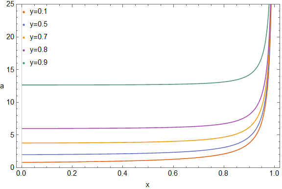
(a) $d=5$, $y$ fixed

(b) $d=5$, $x$ fixed

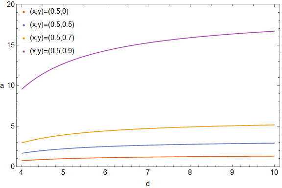
(c) $(x,y)$ fixed

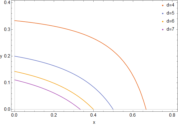
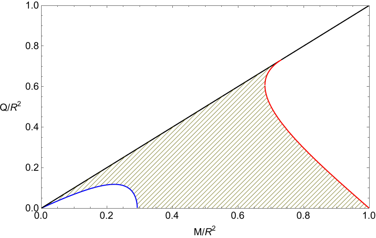
(d) $a=1$

Figure 1: Thermodynamic stability of the shell considering only mass fluctuations is described, see Sec. IV.4 and Eqs. (67), (68) and (81). Plots of $S_{1}\left(d,a,x,y\right)=0$ with $d$ being the number of spacetime dimensions, $a$ being the exponent of the equation of state of the shell, $x=\frac{r_{+}^{d-3}}{R^{d-3}}$, and $y=\frac{r_{-}^{d-3}}{r_{+}^{d-3}}$, where $r_{+}$ and $r_{-}$ are the gravitational radius and the Cauchy radius of the Reissner-Nordström shell spacetime, respectively, and $R$ is the radius of the shell, are shown. The equality $S_{1}\left(d,a,x,y\right)=0$ describes marginal stability of the shell considering only mass fluctuations. (a) The function is plotted as $a(x)$ with $d=5$ and for fixed values of $y$, with points with lower $a$ than the function corresponding to stable configurations; (b) The function is plotted as $a(y)$ with $d=5$ and for fixed values of $x$, with points with lower $a$ corresponding to stable configurations; (c) The function is plotted as $a(d)$ for fixed values of the pair $(x,y)$, with points with lower $a$ corresponding to stable configurations; (d) In the top plot, for $a=1$ with fixed values of $d$ the function is plotted as $y(x)$, with configurations with higher $x$ than the curve being stable; in the bottom plot, one uses the the function in the form $S_{1}\left(d=5,a=1,\frac{M}{R},\frac{Q}{R}\right)=0$, where $M$ is the rest mass of the shell and $Q$ is the charge of the shell, see Sec. IV.11 and Eq. (81), to plot, for $a=1$ with $\mu=1$ and $d=5$, the function $Q(M)$ in the blue curve, the region of stability in the yellow line filled area, $Q=M$ in the black line, and $r_{+}=R$ in the red curve.

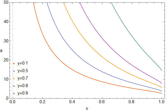
(a) $d=5$, $y$ fixed

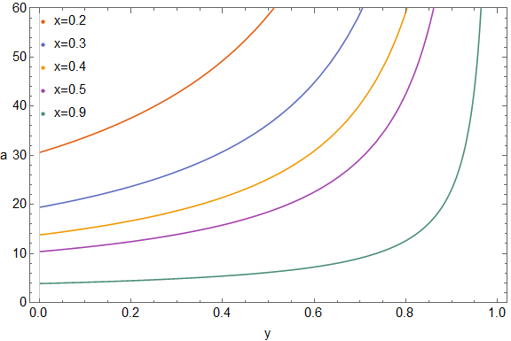
(b) $d=5$, $x$ fixed

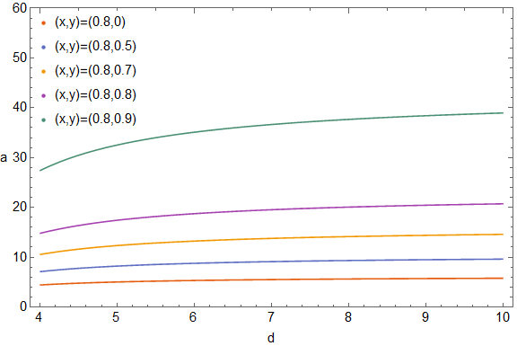
(c) $(x,y)$ fixed

Figure 2: Thermodynamic stability of the shell considering only area fluctuations is described, see Sec. IV.5 and Eqs. (69) and (70). Plots of $S_{2}\left(d,a,x,y\right)=0$, with $d$ being the number of spacetime dimensions, $a$ being the exponent of the equation of state of the shell, $x=\frac{r_{+}^{d-3}}{R^{d-3}}$, and $y=\frac{r_{-}^{d-3}}{r_{+}^{d-3}}$, where $r_{+}$ and $r_{-}$ are the gravitational radius and the Cauchy radius of the Reissner-Nordström shell spacetime, respectively, and $R$ is the radius of the shell, are shown. The equality $S_{2}\left(d,a,x,y\right)=0$ describes marginal stability of the shell considering area fluctuations only. (a) The function is plotted as $a(x)$ with $d=5$ and for fixed values of $y$; (b) The function is plotted as $a(y)$ with $d=5$ and for fixed values of $x$; (c) The function is plotted as $a(d)$ for fixed values of the pair $(x,y)$. Points with lower $a$ than the given function correspond to stable configurations in all three plots. All the configurations with $a=1$ are below the surface of marginal stability, therefore they are stable so there is no need for a plot (d).

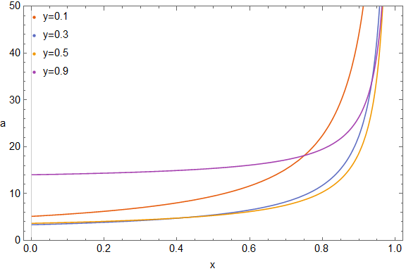
(a) $d=5$, $y$ fixed

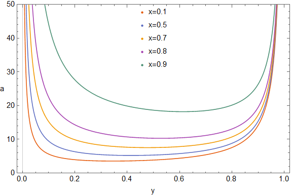
(b) $d=5$, $x$ fixed

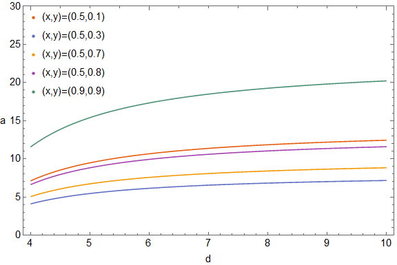
(c) $(x,y)$ fixed

Figure 3: Thermodynamic stability of the shell considering only charge fluctuations is described, see Sec. IV.6 and Eqs. (71) and (72). Plots of $S_{3}\left(d,a,x,y\right)=0$, with $d$ being the number of spacetime dimensions, $a$ being the exponent of the equation of state of the shell, $x=\frac{r_{+}^{d-3}}{R^{d-3}}$, and $y=\frac{r_{-}^{d-3}}{r_{+}^{d-3}}$, where $r_{+}$ and $r_{-}$ are the gravitational radius and the Cauchy radius of the Reissner-Nordström shell spacetime, respectively, and $R$ is the radius of the shell, are shown. The equality $S_{3}\left(d,a,x,y\right)=0$ describes marginal stability of the shell considering charge fluctuations only. (a) The function is plotted as $a(x)$ with $d=5$ and for fixed values of $y$; (b) The function is plotted as $a(y)$ with $d=5$ and for fixed values of $x$; (c) The function is plotted as $a(d)$ for fixed values of the pair $(x,y)$. Points with lower $a$ than the given function correspond to stable configurations in all three plots. All the configurations with $a=1$ are below the surface of marginal stability, therefore they are stable so there is no need for a plot (d).

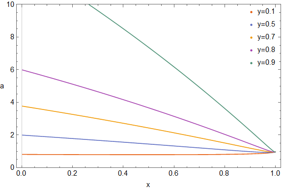
(a) $d=5$, $y$ fixed

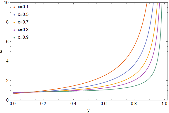
(b) $d=5$, $x$ fixed

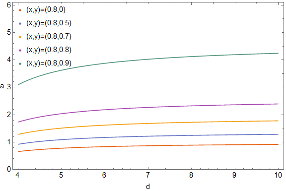
(c) $(x,y)$ fixed

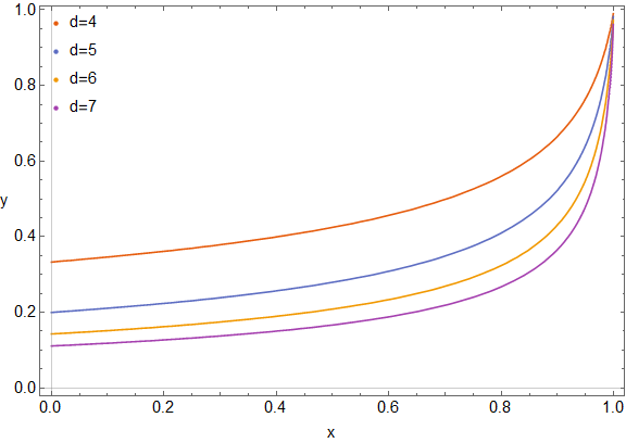
(d) $a=1$

Figure 4: Thermodynamic stability of the shell considering mass and area fluctuations together is described, see Sec. IV.7 and Eqs. (73) and (74). Plots of $S_{4}\left(d,a,x,y\right)=0$, with $d$ being the number of spacetime dimensions, $a$ being the exponent of the equation of state of the shell, $x=\frac{r_{+}^{d-3}}{R^{d-3}}$, and $y=\frac{r_{-}^{d-3}}{r_{+}^{d-3}}$, where $r_{+}$ and $r_{-}$ are the gravitational radius and the Cauchy radius of the Reissner-Nordström shell spacetime, respectively, and $R$ is the radius of the shell, are shown. The equality $S_{4}\left(d,a,x,y\right)=0$ describes marginal stability of the shell considering together mass and area fluctuations. (a) The function is plotted as $a(x)$ with $d=5$ and for fixed values of $y$, with points with lower $a$ than the function corresponding to stable configurations; (b) The function is plotted as $a(y)$ with $d=5$ and for fixed values of $x$, with points with lower $a$ corresponding to stable configurations; (c) The function is plotted as $a(d)$ for fixed values of the pair $(x,y)$, with points with lower $a$ corresponding to stable configurations; (d) The function is plotted as $y(x)$ for $a=1$ with fixed values of $d$, with configurations with higher $x$ than the curve being stable.

Appendix D Laboratory variables: Details for Sec. V

D.1 Mass and charge fluctuations together: Second derivatives of the entropy in terms of laboratory quantities

Here we show the detailed calculations of the stability conditions in terms of laboratory quantities presented in Sec. V.2 for the study of mass and charge fluctuations together. The idea is that the second derivatives of the entropy can be written in terms of variables that one can measure in the laboratory, i.e., thermodynamic coefficients. We start from the two equations of state $dT$ and $d\Phi$, seen as functions of $S$, $A$, and $Q$. They are given by

$$dT=\frac{T}{C_{A,Q}}dS-T\frac{\lambda_{T,Q}}{C_{A,Q}}dA-\frac{T\lambda_{T,A}}{C_{A,Q}}dQ\,,$$ (101)

$$d\Phi=-\frac{T\lambda_{T,A}}{C_{A,Q}}dS+P_{S,Q}dA+\frac{1}{\chi_{S,A}}dQ\,,$$ (102)

where $C_{A,Q}$ is the specific heat capacity at constant area and electric charge, $\lambda_{T,Q}$ is the latent heat capacity at constant temperature and charge associated to the area, $\lambda_{T,A}$ is the latent heat capacity at constant temperature and area associated to the charge, $P_{S,Q}$ is the electric pressure at constant entropy and charge, and $\chi_{S,A}$ is the adiabatic electric susceptibility at constant area. We then write the differentials $dT(M,A,Q)$ and $d\Phi(M,A,Q)$ by using Eq. (36), i.e., $TdS=dM+pdA-\Phi dQ$, in Eqs. (101) and (102), yielding

$$dT= \frac{1}{C_{A,Q}}dM-\frac{T\lambda_{T,A}+\Phi}{C_{A,Q}}dQ-\frac{T\lambda_{T,Q}-p}{C_{A,Q}}dA\,,$$ (103)

$$d\Phi= -\frac{\lambda_{T,A}}{C_{A,Q}}dM+\left(\frac{1}{\chi_{S,A}}+\frac{\Phi\lambda_{T,A}}{C_{A,Q}}\right)dQ$$

$$+\left(\frac{\kappa_{p,S}}{\kappa_{S,Q}}-p\frac{\lambda_{T,A}}{C_{A,Q}}\right)dA\,.$$ (104)

Now, Eq. (36), i.e., $TdS=dM+pdA-\Phi dQ$, and Eq. (103), yield $S_{MM}=-\beta^{2}\left(\frac{\partial T}{\partial M}\right)_{A,Q}=-\beta^{2}C_{A,Q}^{-1}$. Thus, the first condition for stability, $S_{MM}\leq 0$, can be written as $C_{A,Q}^{-1}\geq 0$, or equivalently,

$$C_{A,Q}\geq 0\,.$$ (105)

In addition, one can write $S_{MM}S_{QQ}-S_{MQ}^{2}$ as $S_{MM}S_{QQ}-S_{MQ}^{2}=-\left(\frac{\partial\beta}{\partial M}\right)_{A,Q}\left(\frac{\partial\beta\Phi}{\partial Q}\right)_{M,A}-\left(\frac{\partial\beta}{\partial Q}\right)_{M,A}^{2}=-\beta^{4}\left(\frac{\partial T}{\partial M}\right)_{A,Q}\left(\frac{\partial T}{\partial Q}\right)_{M,A}\Phi-\beta^{3}\left(\frac{\partial T}{\partial M}\right)_{A,Q}\left(\frac{\partial\Phi}{\partial Q}\right)_{M,A}-\beta^{4}\left(\frac{\partial T}{\partial Q}\right)_{M,A}^{2}$, where Eq. (36), i.e., $TdS=dM+pdA-\Phi dQ$, has been of help. Then, putting Eqs. (103) and (104) into this latter equation, one finds $S_{MM}S_{QQ}-S_{MQ}^{2}=\beta^{3}\left(\frac{1}{C_{A,Q}\chi_{S,A}}-\frac{T\lambda_{T,A}^{2}}{C_{A,Q}^{2}}\right)$. Thus, the second and necessary condition for stability, namely, $S_{MM}S_{QQ}-S_{MQ}^{2}\geq 0$, can be written as

$$\beta^{3}\left(\frac{1}{C_{A,Q}\chi_{S,A}}-\frac{T\lambda_{T,A}^{2}}{C_{A,Q}^{2}}\right)\geq 0\,.$$ (106)

This can be further simplified. If we introduce the heat capacity at constant electric potential and constant area, $C_{A,\Phi}=T\left(\frac{\partial S}{\partial T}\right)_{\Phi,A}$. This coefficient can be written as $C_{A,\Phi}^{-1}=\beta\left(\frac{\partial T}{\partial S}\right)_{A,\Phi}=\beta\left(\left(\frac{\partial T}{\partial S}\right)_{Q,A}+\left(\frac{\partial T}{\partial Q}\right)_{S,A}\left(\frac{\partial Q}{\partial S}\right)_{\Phi,A}\right)=\beta C_{A,Q}^{-1}\left(1-\frac{T\lambda_{T,A}^{2}}{C_{A,Q}}\chi_{S,A}\right)=\beta\chi_{S,A}\left(\frac{1}{C_{A,Q}\chi_{S,A}}-\frac{T\lambda_{T,A}^{2}}{C_{A,Q}^{2}}\right)$, where we have used Eqs. (101) and (102) to compute the derivatives. Also, we used that $\left(\frac{\partial Q}{\partial S}\right)_{\Phi,A}=T\chi_{S,A}\frac{\lambda_{T,A}}{C_{A,Q}}$, that comes from inverting Eq. (102) to obtain $dQ(S,A,\Phi)$. Thus, $\beta^{3}\left(\frac{1}{C_{A,Q}\chi_{S,A}}-\frac{T\lambda_{T,A}^{2}}{C_{A,Q}^{2}}\right)=\beta^{2}\frac{1}{C_{A,\Phi}\chi_{S,A}}$, and Eq. (106) can be rewritten as $\frac{1}{C_{A,\Phi}\chi_{S,A}}\geq 0$, or, equivalently, as

$$C_{A,\Phi}\chi_{S,A}\geq 0\,,$$ (107)

which is the upshot of the second condition for stability $S_{MM}S_{QQ}-S_{MQ}^{2}\geq 0$ in the physical variables.

Now, we consider the particular case of the thin shell with the equations of state given by Eqs. (49) and (50). The first condition for stability, Eq. (105), holds without further ado. The second condition for stability, Eq. (107) can be improved for the equations of state used. The coefficient $\chi_{S,A}$ can be calculated using the differential in Eqs. (104) through $\chi_{S,A}^{-1}=\left(\frac{\partial\Phi}{\partial Q}\right)_{M,A}+\Phi\left(\frac{\partial\Phi}{\partial M}\right)_{A,Q}$. The equation of state in consideration is given by Eqs. (46) and (50), $\Phi=Q\left[\frac{r_{+}^{-(d-3)}-R^{-(d-3)}}{1-\frac{\mu M}{R^{d-3}}}\right]$, with $r_{+}=r_{+}(M,A,Q)$ defined by Eqs. (15) and (33). Thus, the coefficient $\chi_{S,A}^{-1}$ for this case is $\chi_{S,A}^{-1}=\Phi^{2}\frac{\mu}{R^{d-3}\left(1-\mu\frac{M}{R^{d-3}}\right)}+\frac{\Phi}{Q}$, which is positive for values of $(M,A,Q)$ that are physical. This means that the second condition for stability given in Eq. (107) is reduced to

$$C_{A,\Phi}\geq 0\,,$$ (108)

for the equations of state we have used.

Here we have deduced in detail the stability conditions in physical variables for mass and charged fluctuations presented in the main text in Sec. V.2. So, Eqs. (103) and (104) are Eqs. (82) and (83) of the main text, respectively, Eqs. (105) and (107) are the two equations given in Eq. (V.2) of the main text, and Eq. (108) is Eq. (85) of the main text.

D.2 Mass, area, and charge fluctuations altogether: Second derivatives of the entropy in terms of laboratory quantities

Here we show the detailed calculations of the stability conditions in terms of laboratory quantities presented in Sec. V.3 for the study of mass, area, and charge fluctuations altogether. The idea is that the second derivatives of the entropy can be written in terms of variables one can measure in the laboratory, i.e., thermodynamic coefficients. We start from the three equations of state $dS(T,p,Q)$, $dA(T,p,Q)$ and $d\Phi(T,p,Q)$, seen as functions of $T$, $p$, and $Q$. They are given by

$$dS= \left(\frac{C_{A,Q}}{T}+A\frac{\alpha_{p,Q}^{2}}{\kappa_{T,Q}}\right)dT$$

$$-A\alpha_{p,Q}dp+\lambda_{p,T}dQ\,,$$ (109)

$$\frac{dA}{A}= \alpha_{p,Q}dT-\kappa_{T,Q}dp-\kappa_{p,T}dQ\,,$$ (110)

$$d\Phi= -\lambda_{p,Q}dT-A\kappa_{p,T}dp+\frac{1}{\chi_{T,p}}dQ\,,$$ (111)

where $C_{A,Q}$ is the heat capacity at constant area and charge, $\alpha_{p,Q}$ is the thermal expansion coefficient, $\kappa_{T,Q}$ is the isothermal compressibility, $\lambda_{p,T}$ is a latent heat capacity, $\kappa_{p,T}$ is the electric compressibility, $\lambda_{p,Q}$ is another latent heat capacity, and $\chi_{T,p}$ is the isothermal electric susceptibility. We can invert Eqs. (109) and (110) to obtain $dT(S,A,Q)$ and $dp(S,A,Q)$. This is accomplished by rewriting Eqs. (109) and (110) in matrix form, i.e.,

$$\begin{pmatrix}dS-\lambda_{p,T}dQ\\ dA+A\kappa_{p,T}dQ\end{pmatrix}=\mathcal{M}\begin{pmatrix}dT\\ dp\end{pmatrix}\,,$$ (112)

where

$$\mathcal{M}=\begin{pmatrix}\left(\frac{C_{A,Q}}{T}+A\frac{\alpha_{p,Q}^{2}}{\kappa_{T,Q}}\right)&-A\alpha_{p,T}\\ A\alpha_{p,Q}&-A\kappa_{T,Q}\end{pmatrix}\,.$$ (113)

The matrix $\mathcal{M}$ can be inverted to yield

$$\mathcal{M}^{-1}=\begin{pmatrix}\frac{T}{C_{A,Q}}&-T\frac{\alpha_{p,Q}}{C_{A,Q}\kappa_{T,Q}}\\ T\frac{\alpha_{p,Q}}{C_{A,Q}\kappa_{T,Q}}&-\left(\frac{1}{A\kappa_{T,Q}}+T\frac{\alpha^{2}_{p,Q}}{\kappa_{T,Q}^{2}C_{A,Q}}\right)\end{pmatrix}\,.$$ (114)

Applying $\mathcal{M}^{-1}$ on both sides of Eq. (112), we obtain $dT(S,A,Q)$ and $dp(S,A,Q)$ as

$$dT= \frac{T}{C_{A,Q}}dS-T\frac{\alpha_{p,Q}}{C_{A,Q}\kappa_{T,Q}}dA-T\mathcal{B}dQ\,,$$ (115)

$$dp= \frac{T\alpha_{p,Q}}{C_{A,Q}\kappa_{T,Q}}dS-\left(\frac{1}{A\kappa_{T,Q}}+T\frac{\alpha_{p,Q}^{2}}{\kappa_{T,Q}^{2}C_{A,Q}}\right)dA$$

$$-\left(\frac{\kappa_{p,T}}{\kappa_{T,Q}}+T\frac{\alpha_{p,Q}}{\kappa_{T,Q}}\mathcal{B}\right)dQ\,,$$ (116)

where $\mathcal{B}=\frac{\lambda_{p,T}}{C_{A,Q}}+A\frac{\alpha_{p,Q}\kappa_{p,T}}{C_{A,Q}\kappa_{T,Q}}$. We can then compute directly $dT(M,A,Q)$ and $dp(M,A,Q)$ by substituting the differential $dS$ given in Eq. (36), i.e., $TdS=dM+pdA-\Phi dQ$, into Eqs. (115) and (116), yielding

$$dT= \frac{dM}{C_{A,Q}}+\left(\frac{p}{C_{A,Q}}-T\frac{\alpha_{p,Q}}{C_{A,Q}\kappa_{T,Q}}\right)dA$$

$$-\left(\frac{\Phi}{C_{A,Q}}+T\frac{\lambda_{p,T}}{C_{A,Q}}+A\frac{\alpha_{p,T}\kappa_{p,T}}{\kappa_{T,Q}C_{A,Q}}\right)dQ\,,$$ (117)

$$dp= \frac{\alpha_{p,Q}}{C_{A,Q}\kappa_{T,Q}}dM$$

$$-\left[\frac{1}{A\kappa_{T,Q}}-\frac{\alpha_{p,Q}}{C_{A,Q}\kappa_{T,Q}}\left(p-T\frac{\alpha_{p,Q}}{\kappa_{T,Q}}\right)\right]dA$$

$$-\left(\frac{\kappa_{p,T}}{\kappa_{T,Q}}-\frac{\alpha_{p,Q}}{C_{A,Q}\kappa_{T,Q}}\mathcal{C}\right)dQ\,,$$ (118)

where $\mathcal{C}=TA\frac{\kappa_{p,T}\alpha_{p,Q}}{\kappa_{T,Q}}+T\lambda_{p,T}+\Phi$. Then, substituting $dT$ and $dp$ given in Eqs. (115) and (116), respectively, into $d\Phi(T,p,Q)$, written in Eq. (111), we obtain

$$d\Phi= -\mathcal{B}dM+\left[\frac{\kappa_{p,T}}{\kappa_{T,Q}}-\left(p-T\frac{\alpha_{p,Q}}{\kappa_{T,Q}}\right)\mathcal{B}\right]dA$$

$$+\left(\mathcal{B}\mathcal{C}+\frac{1}{\chi_{p,T}}+A\frac{\kappa_{p,T}^{2}}{\kappa_{T,Q}}\right)dQ\,.$$ (119)

With $dT(M,A,Q)$, $dp(M,A,Q)$ and $d\Phi(M,A,Q)$, we can write the second derivatives of the entropy since these are derivatives of $\beta(M,A,Q)$, $\beta p(M,A,Q)$ and $\beta\Phi(M,A,Q)$. The second derivatives are explicitly $S_{MM}=-\frac{\beta^{2}}{C_{A,Q}}$, $S_{AA}=-\left[\frac{1}{A\kappa_{T,Q}}+\frac{\beta^{2}}{C_{A,Q}}\left(p-T\frac{\alpha_{p,Q}}{\kappa_{T,Q}}\right)^{2}\right]$, $S_{QQ}=-\beta\left[\frac{\mathcal{C}^{2}\beta}{C_{A,Q}}+\frac{1}{\chi_{p,T}}+A\frac{\kappa_{p,T}^{2}}{\kappa_{T,Q}}\right]$, $S_{MA}=\frac{\beta^{2}}{C_{A,Q}}\left(T\frac{\alpha_{p,Q}}{\kappa_{T,Q}}-p\right)$, $S_{MQ}=\frac{\beta^{2}}{C_{A,Q}}\mathcal{C}$, $S_{AQ}=-\beta\left[\frac{\kappa_{p,T}}{\kappa_{T,Q}}-\frac{\beta^{2}}{C_{A,Q}}\left(p-T\frac{\alpha_{p,Q}}{\kappa_{T,Q}}\right)\mathcal{C}\right]$. Thus, the relevant combinations of the second derivatives for the stability conditions are $S_{MM}=-\frac{\beta^{2}}{C_{A,Q}}$, $S_{MM}S_{AA}-S_{MA}^{2}=\frac{\beta^{3}}{AC_{A,Q}\kappa_{T,Q}}$, and $(S_{MM}S_{AQ}-S_{MA}S_{MQ})^{2}-(S_{MM}S_{AA}-S_{MA}^{2})(S_{MM}S_{QQ}-S_{MQ}^{2})=-\frac{\beta^{6}}{AC_{A,Q}^{2}\kappa_{T,Q}\chi_{p,T}}$. For stability one has $S_{MM}\leq 0$, $S_{MM}S_{AA}-S_{MA}^{2}\geq 0$, and $(S_{MM}S_{AQ}-S_{MA}S_{MQ})^{2}-(S_{MM}S_{AA}-S_{MA}^{2})(S_{MM}S_{QQ}-S_{MQ}^{2})\leq 0$, which translates into

$$C_{A,Q}\geq 0,\,$$ (120)

$$\kappa_{T,Q}\geq 0\,,$$ (121)

$$\chi_{p,T}\geq 0\,.$$ (122)

These are the stability conditions for mass, area, and charge fluctuations. In words, the heat capacity at constant area and charge, the isothermal compressibility associated to the pressure, and the isothermal electric susceptibility must be positive.

The particular case of the thin shell with the equations of state given by Eqs. (49), (50), and (30) can be also worked out in detail, we will not do it here.

Here, we have deduced in detail the stability conditions in physical variables for mass, area, and charged fluctuations presented in the main text in Sec. V.3. So, Eqs. (117) and (118) are Eqs. (86) and (87) of the main text, respectively, Eq. (119) is Eq. (88) of the main text, and Eqs. (120), (121), (122) are the three equations given in Eq. (89) of the main text.

References

• (1) W. Israel, “Gravitational collapse and causality”, Phys. Rev. 153, 1388 (1967).
• (2) K. Kuchař, “Charged shells in general relativity and their gravitational collapse”, Czech. J. Phys. B 18, 435 (1968).
• (3) J. Kijowski and E. Czuchry “Dynamics of a self-gravitating shell of matter”, Phys. Rev. D 72, 084015 (2005); arXiv:gr-qc/0507074.
• (4) G. A. S. Dias, S. Gao, and J. P. S. Lemos, “Charged shells in Lovelock gravity: Hamiltonian treatment and physical implications”, Phys. Rev. D 75, 024030 (2007); arXiv:gr-qc/0612072.
• (5) S. Gao and J. P. S. Lemos, “Collapsing and static thin massive charged dust shells in a Reissner-Nordstrom black hole background in higher dimensions”, Int. J. Mod. Phys. A 23 , 2943 (2008); arXiv:0804.0295 [hep-th].
• (6) E. F. Eiroa and C. Simeone, “Aspects of spherical shells in a $d$-dimensional background”, Int. J. Mod. Phys. D 21, 1250033 (2012); arXiv:1202.5009 [gr-qc].
• (7) H. Andréasson, “Sharp bounds on the critical stability radius for relativistic charged spheres”, Commun. Math. Phys. 288, 715 (2009); arXiv:0804.1882 [gr-qc]
• (8) J. P. S. Lemos and P. Luz, “All fundamental electrically charged thin shells in general relativity: From star shells to tension shell black holes, regular black holes, and beyond”, Phys. Rev. D 103, 104046 (2021); arXiv:2103.15832 [gr-qc].
• (9) G. A. S. Dias and J. P. S. Lemos, “Thin-shell wormholes in $d$-dimensional general relativity: Solutions, properties, and stability”, Phys. Rev. D 82, 084023 (2010); arXiv:1008.3376 [gr-qc].
• (10) C. Bejarano and E. F. Eiroa, “Dilaton thin-shell wormholes supported by a generalized Chaplygin gas”, Phys. Rev. D 84, 064043 (2011); arXiv:1106.6340 [gr-qc].
• (11) J. P. S. Lemos and P. Luz, “Bubble universes and traversable wormholes”, Phys. Rev. D 105, 044058 (2022); arXiv:2201.02203 [gr-qc].
• (12) J. P. S. Lemos and V. T. Zanchin, “Regular black holes: Electrically charged solutions, Reissner-Nordström outside a de Sitter core”, Phys. Rev. D 83, 124005 (2011); arXiv:1104.4790 [gr-qc].
• (13) N. Uchikata, S. Yoshida, and T. Futamase, “New solutions of charged regular black holes and their stability”, Phys. Rev. D 86, 084025 (2012); arXiv:1209.3567 [gr-qc].
• (14) R. Brandenberger, L. Heisenberg, and J. Robnik, “Non-singular black holes with a zero-shear S-brane”, J. High Energy Phys. JHEP 05 (2021) 090; arXiv:2103.02842 [hep-th].
• (15) E. A. Martinez, “Fundamental thermodynamical equation of a self-gravitating system”, Phys. Rev. D 53, 7062 (1996).
• (16) S. E. Perez Bergliaffa, M. Chiapparini, and L. M. Reyes, “Thermodynamical and dynamical stability of a self-gravitating uncharged thin shell”, Eur. Phys. J. C 80, 719 (2020); arXiv:2006.06766 [gr-qc].
• (17) R. André, J. P. S. Lemos, and G. M. Quinta, “Thermodynamics and entropy of self-gravitating matter shells and black holes in $d$ dimensions”, Phys. Rev. D 99, 125013 (2019); arXiv:1905.05239 [hep-th].
• (18) J. P. S. Lemos, G. M. Quinta, and O. B. Zaslavskii, “Entropy of a self-gravitating electrically charged thin shell and the black hole limit”, Phys. Rev. D 91, 104027 (2015); arXiv:1503.00018 [hep-th].
• (19) L. M. Reyes, M. Chiapparini, and S. E. Perez Bergliaffa, “Thermodynamical and dynamical stability of a self-gravitating charged thin shell”, Eur. Phys. J. C 82, 151 (2022).
• (20) J. P. S. Lemos, G. M. Quinta, and O. B. Zaslavskii, “Entropy of an extremal electrically charged thin shell and the extremal black hole”, Phys. Lett. B 750, 306 (2015); arXiv:1505.05875 [hep-th].
• (21) J. P. S. Lemos, G. M. Quinta, and O. B. Zaslavskii, “Entropy of extremal black holes: Horizon limits through charged thin shells, a unified approach”, Phys. Rev. D 93, 084008 (2016); arXiv:1603.01628 [hep-th].
• (22) J. W. York, “Black hole thermodynamics and the Euclidean Einstein action”, Phys. Rev. D 33, 2092 (1986).
• (23) O. B. Zaslavskii, “Canonical ensemble for arbitrary configurations of self-gravitating systems”, Phys. Lett. A 152, 463 (1991).
• (24) R. André and J. P. S. Lemos, “Thermodynamics of five-dimensional Schwarzschild black holes in the canonical ensemble”, Phys. Rev. D 102, 024006 (2020); arXiv:2006.10050 [hep-th].
• (25) R. André and J. P. S. Lemos, “Thermodynamics of $d$-dimensional Schwarzschild black holes in the canonical ensemble”, Phys. Rev. D 103, 064069 (2021); arXiv:2101.11010 [hep-th].
• (26) E. A. Martinez and J. W. York, “Additivity of the entropies of black holes and matter in equilibrium”, Phys. Rev. D 40, 2124 (1989).
• (27) H. W. Braden, J. D. Brown, B. F. Whiting, and J. W. York, “Charged black hole in a grand canonical ensemble”, Phys. Rev. D 42, 3376 (1990).
• (28) C. S. Peça and J. P. S. Lemos, “Thermodynamics of Reissner-Nordström-anti-de Sitter black holes in the grand canonical ensemble”, Phys. Rev. D 59, 124007 (1999); arXiv:gr-qc/9805004.
• (29) J. P. S. Lemos and O. B. Zaslavskii, “Quasiblack holes: Definition and general properties”, Phys. Rev. D 76, 084030 (2007); arXiv:0707.1094 [gr-qc].
• (30) J. P. S. Lemos and O. B. Zaslavskii, “Entropy of quasiblack holes”, Phys. Rev. D 81, 064012 (2010); arXiv:0904.1741 [gr-qc].
• (31) J. P. S. Lemos and O. B. Zaslavskii, “Entropy of extremal black holes from entropy of quasiblack holes”, Phys. Lett. B 695, 37 (2011).
• (32) J. P. S. Lemos and O. B. Zaslavskii, “Compact objects in general relativity: From Buchdahl stars to quasiblack holes”, Int. J. Mod. Phys. D 29, 2041019 (2020); arXiv:2007.00665 [gr-qc].
• (33) H. B. Callen, Thermodynamics and an Introduction to Thermostatistics, 2nd ed. (Wiley, New York, 1991).