Limits of Entrainment
of Circadian Neuronal Networks

Abstract

Circadian rhythmicity lies at the center of various important physiological and behavioral processes in mammals, such as sleep, metabolism, homeostasis, mood changes and more. It has been shown that this rhythm arises from self-sustained biomolecular oscillations of a neuronal network located in the Suprachiasmatic Nucleus (SCN). Under normal circumstances, this network remains synchronized to the day-night cycle due to signaling from the retina. Misalignment of these neuronal oscillations with the external light signal can disrupt numerous physiological functions and take a long-lasting toll on health and well-being. In this work, we study a modern computational neuroscience model to determine the limits of circadian synchronization to external light signals of different frequency and duty cycle. We employ a matrix-free approach to locate periodic steady states of the high-dimensional model for various driving conditions. Our algorithmic pipeline enables numerical continuation and construction of bifurcation diagrams w.r.t. forcing parameters. We computationally explore the effect of heterogeneity in the circadian neuronal network, as well as the effect of corrective therapeutic interventions, such as that of the drug molecule Longdaysin. Lastly, we employ unsupervised learning to construct a data-driven embedding space for representing neuronal heterogeneity.

It is long known that the human brain not only keeps time, but adapts its own clock to the day-night (circadian) cycle. This is achieved when an internal, “default” rhythm synchronizes with the external, forcing cycle of alternating light and darkness. In this work, this synchronization phenomenon is computationally studied, using a detailed model of the group of neurons that constitute the circadian clock. We employ tools from nonlinear dynamics to estimate the limiting conditions under which such synchronization is possible; and what happens when it is not. We also investigate how a certain drug molecule can affect the ability of the circadian clock to synchronize. The algorithms employed are well suited for the complexity of this problem: matrix free simulator-based solvers that efficiently handle high-dimensional equation systems and unsupervised learning techniques that explore heterogeneity in such networks.

I Introduction

The principal circadian pacemaker is located in the two Suprachiasmatic Nuclei of the anterior hypothalamus. The SCN directly receives input from photosensitive cells of the retina via the retinohypothalamic tract Ma and Morrison (2022); Hastings, Maywood, and Brancaccio (2018) while it is also connected to the pineal gland, inducing melatonin production during the night Sack et al. (2007a); Ma and Morrison (2022). The SCN also coordinates secondary cellular pacemakers across the body by controlling biochemical (e.g. neuroendocrine) signals that entrain them Hastings, Maywood, and Brancaccio (2018).

This orchestrating role puts SCN neuronal networks at the center of numerous physiological processes and, consequently, its dysfunction gives rise to numerous disorders. Circadian desynchrony is linked to sleep disorders (jet lag disorder, shift work disorder, advanced sleep phase disorder, delayed sleep phase disorder, free-running disorder, irregular sleep-wake rhythm) Sack et al. (2007a, b), cardiovascular disease, obesity, hypertension Scheer et al. (2009), nephropathy Nakano et al. (1991), cancer Savvidis and Koutsilieris (2012), depression and bipolar disorder Germain and Kupfer (2008); Vadnie and McClung (2017).

Many pharmacological interventions have been suggested to correct misalignments of the circadian rhythm with the external day-night signal. Benzodiazepines and melatonin have been popular choices Turek and Losee-Olson (1986); Sack et al. (2000). As the understanding of the the exact biochemical processes involved deepens, more targeted therapies are developed. Small molecules like Longdaysin (CAS No. : 1353867-91-0) have been extensively studied (in vitro and in silico) as therapeutics in circadian rhythm disorders, as they directly intervene to the gene regulatory network giving rise to the oscillations Huang et al. (2020); St. John et al. (2014); Hirota et al. (2012).

In this work, we use advanced algorithms from numerical analysis/scientific computation and nonlinear dynamics to investigate the ability of SCN neurons and SCN neuronal networks to synchronize with the external day-night signal (in dynamics terms, with the external forcing). Specifically, we explore entrained periodic solutions of high dimensional dynamical systems arising from computational biology models, with respect to different:

1. Forcing angular frequencies $\omega_{f},$ where $\omega_{f}=\frac{2\pi}{T_{f}},$ for a forcing period $T_{f}$ of the day-night (light-dark) cycle.

2. Forcing duty cycles $\phi,$ where $\phi=\frac{T_{light}}{T_{f}}$ for a day duration of $T_{light}$.

3. Simulated Longdaysin effects.

4. Network Heterogeneity extents.

For this purpose, several informative bifurcation diagrams are constructed and the extracted bifurcation points demarcate the limits of entrainment of circadian neurons or neuronal networks. Moreover, we construct a reduced, data-driven “emergent space” description of neuronal behavior heterogeneity using unsupervised learning.

The rest of the manuscript is organized as follows: Section II includes all necessary information for the computational model used. Then, in Section III the main algorithms used are outlined and put into the context of circadian entrainment. Section IV presents our results, and Section V our conclusions.

II Computational Model

The computational model used here is adapted from the work of Vasalou et al. Vasalou, Herzog, and Henson (2011); Vasalou and Henson (2011). They constructed a state-of-the-art computational model of circadian neuronal networks by coupling three components:

1. Biomolecular clock: The computational model of the biomolecular clock was developed by Leloup and Goldbeter Leloup and Goldbeter (2003, 2004) and describes the regulatory loops involving the Per, Cry, Bmal1, Clock and Erv-Erb$\alpha$ genes. The interaction of these loops gives rise to circadian oscillations.

2. Electrophysiology dynamics: This component describes the membrane dynamics of circadian neurons and the way they are coupled with neurotransmitter signaling i.e. with $\gamma$-aminobutyric acid (GABA) and vasoactive intestinal polypeptide (VIP) signaling To et al. (2007); Vasalou and Henson (2011). The firing frequency is incorporated in the model by associating membrane voltage and ion conductances with circadian gene expression Vasalou and Henson (2010).

3. Network connectivity: An ensemble of 425 neurons was chosen for a realistic representation of the SCN circadian network Vasalou and Henson (2011). All neurons are linked via VIP and GABA neurotransmitter networks generated from a small-world architecture resembling neuron connectivities in the SCN Vasalou and Henson (2011) (see Fig.1 for example).

Henson Henson (2013) provides a review comparing this model with others in the literature. There is also experimental evidence supporting the model’s validity Vasalou and Henson (2011); Leloup and Goldbeter (2003).

In this model, the day-night (light-dark) cycle is modeled as a step function with period $T_{f}=T_{light}+T_{dark}$ and duty cycle $\phi=\frac{T_{light}}{T_{f}}$. Light forcing is incorporated in the dynamical system implicitly, by assuming that during the light phase, the AMPA/NDMA and VPAC2 receptors are saturated (in term of model functions: $b_{Glu_{R}}(t)=1,b_{VIP}(t)=1$ for $t\in[0,T_{light}]$) Vasalou and Henson (2011). In contrast to Vasalou et al. Vasalou and Henson (2011) we assume that the photic effect is uniform across all SCN (both core and shell) neurons.

The effect of Longdaysin can also be incorporated in the model. Longdaysin is a small drug molecule acting as a casein kinase I (CKI) inhibitor. It is hypothesized to increase the time required before the Per-Cry complex can enter the nucleus to repress transcription Hirota et al. (2012); St. John et al. (2014). In our model, this effect can be simulated by different values of the parameter $k_{1}$, the nuclear entry rate of phosphorylated Per-Cry complex St. John et al. (2014). Therefore, in our studies, increased values of Longdaysin translate to lower values of $k_{1}$. Note that, here, we assume that the concentration of Longdaysin is constant and not subject to pharmacodynamics.

The realization of the circadian network studied here includes heterogeneity in the parameter $v_{sP_{0}}$, the basal transcription rate of the Per mRNA, across the neurons. This parameter has been shown to strongly affect the ability of circadian neurons to sustain intrinsic oscillations, while the rhythmic phenotype of Per has been shown experimentally to vary Yamaguchi et al. (2003). Specifically, $v_{sP_{0}}$ has been sampled from $\mathcal{N}(1.2,\sigma^{2})$, similarly to Vasalou, Herzog, and Henson (2011) (see Fig.1 for example). It is important to mention, that for reproducibility, the random seed used to generate $v_{sP_{0}}$ and the small-world networks is always fixed.

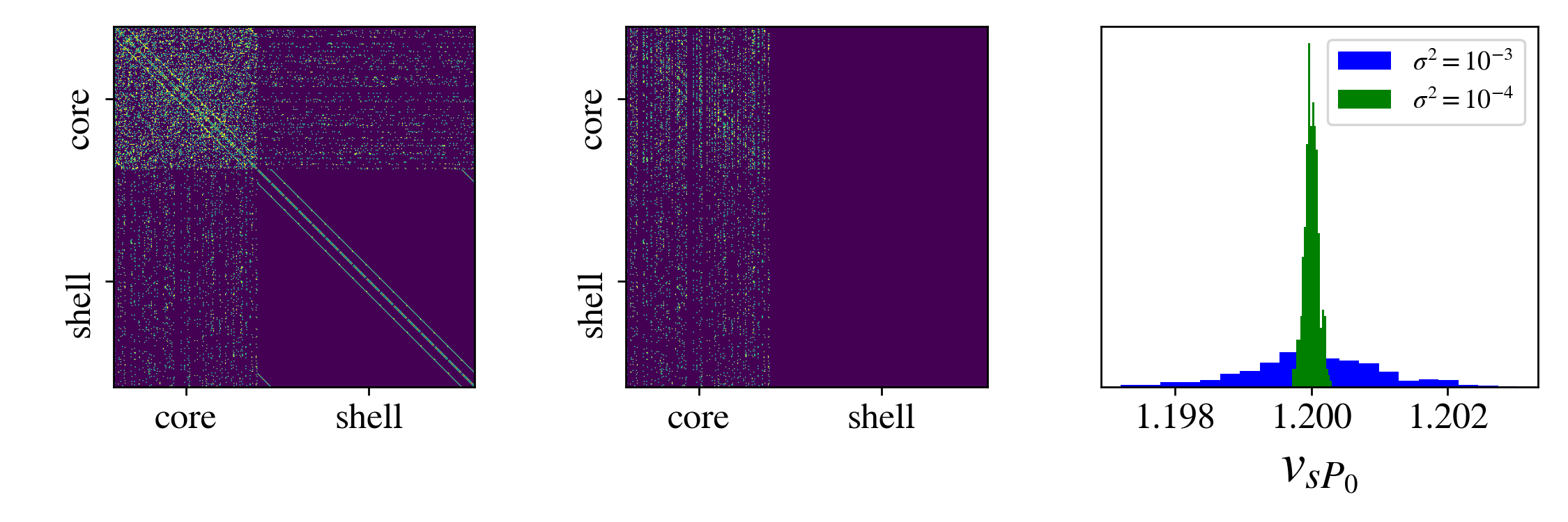
Figure 1: (left) GABA adjacency matrix, (middle) VIP adjacency matrix, (right) histograms sampled from different $v_{sP_{0}}$ considered here.

Putting all components together, each circadian neuron is described by 21 Ordinary Differential Equations (ODEs), each of which describes the time evolution of a relevant chemical species. When the entire network is simulated, the resulting system is 8925-dimensional.

III Algorithms for computing synchronization of large oscillating networks

III.1 Stroboscopic Map

The studied model is a periodically forced dynamical system, and computations are performed using a stroboscopic map, i.e., we evaluate the periodic solution at a selected, fixed phase of the forcing term Kevrekidis, Schmidt, and Aris (1986). This acts as a natural pinning condition: the period of forced oscillations is, by necessity, an integer multiple of the period of the forcing term. This is why the term “entrainment” (of the oscillator by the forcing) is used.

The dynamics of the problem are described by a system of ODEs, which has the general form:

$$\frac{\textrm{d}\bf{X}}{\textrm{d}t}=\mathbf{f}\left(\mathbf{X}(t);\lambda\right),$$ (1)

where $\bf{X}$ denotes the state vector, and $\lambda$ is a parameter of the system. To compute a periodic solution at a given period $T_{f}$, we seek $\mathbf{X}(0)$ satisfying:

$$\mathbf{R}\coloneqq\mathbf{X}(0)-\mathbf{X}(T_{f})=\mathbf{X}(0)-\bm{\Phi}_{T_{f}}\left(\mathbf{X}(0);\lambda\right),$$ (2)

with $\bm{\Phi}_{T_{f}}$ denoting the temporal evolution operator of the system that reports the solution after a time interval $T_{f}$.

One converges computationally to a periodic solution employing the Newton-Raphson iterative technique, which solves at each iteration the linearized system:

$$\left[\mathbf{I}-\frac{\partial\bm{\Phi}_{T_{f}}}{\partial\mathbf{X}(0)}\right]\delta\mathbf{X}(0)=-\left[\mathbf{X}(0)-\bm{\Phi}_{T_{f}}\left(\mathbf{X}(0)\right)\right]$$ (3)

and updates $\mathbf{X}(0)$ with $\mathbf{X}(0)+\delta\mathbf{X}(0)$ until convergence. Here, the computation of the variational matrix, $\mathbf{V}(t)\coloneqq\Large{\frac{\partial\bm{\Phi}_{T_{f}}}{\partial\mathbf{X}(0)}}$ requires the solution of the following set of ODEs:

$$\frac{\textrm{d}\mathbf{V}}{\textrm{d}t}=\mathbf{J}\cdot\mathbf{V},$$ (4)

where $\mathbf{J}$ is the Jacobian of $\mathbf{f}$, $\mathbf{J}\coloneqq\frac{\partial\bf{f}}{\partial\bf{X}}$, and initial condition: $\mathbf{V}(t=0)=\mathbf{I}$. When the Jacobian’s analytical derivation is nontrivial, one can resort to numerical approximations by calling the time stepper $\bm{\Phi}_{T_{f}}$ at appropriately perturbed values of the unknowns. This approach would be, however, impractical for large-scale problems. For this reason, Eq. 3 is solved with matrix-free iterative solvers, such as the Newton-GMRES (Generalized Minimum Residual) method Saad and Schultz (1986); Kelley, Kevrekidis, and Qiao (2004); Dickson et al. (2007); Vandekerckhove, Kevrekidis, and Roose (2009).

III.2 Matrix-Free Newton-GMRES

The decisive advantage of Newton-GMRES is that the explicit calculation and storage of the Jacobian of the fixed point problem is not required; instead, the action of the Jacobian on systematically selected vectors is approximated numerically. We only require matrix-vector multiplications, that can be estimated at low cost by calling $\bm{\Phi}_{T_{f}}$ from appropriately perturbed initial conditions Kelley (2003); Siettos, Pantelides, and Kevrekidis (2003). In particular, to solve Eq. (3) iteratively with GMRES, one estimates the directional derivative of $\bm{\Phi}_{T_{f}}$ on known vectors, $\mathbf{q}$:

$$\frac{\partial\bm{\Phi}_{T_{f}}}{\partial\mathbf{X}(0)}\cdot\mathbf{q}\approx\frac{\bm{\Phi}_{T_{f}}\left(\mathbf{X}(0)+\epsilon\mathbf{q}\right)-\bm{\Phi}_{T_{f}}\left(\mathbf{X}(0)\right)}{\epsilon},$$ (5)

where $\epsilon$ is a small and appropriately chosen scalar. Such matrix-vector multiplications are required to construct the $j-$th Krylov subspace, which for this problem is:

$$K_{j}=K_{j}(\mathbf{A},r_{o})=\textrm{span}\left\{r_{o},\mathbf{A}r_{o},...,\mathbf{A}^{j-1}r_{o}\right\},$$ (6)

where:

$$\mathbf{A}=\mathbf{I}-\frac{\partial\bm{\Phi}_{T_{f}}}{\partial\mathbf{X}(0)},\hskip 5.69046ptr_{o}=-\left[\mathbf{X}(0)-\bm{\Phi}_{T_{f}}\left(\mathbf{X}(0)\right)\right],$$ (7)

with $r_{o}$ being the initial error given that the initial guess to solve Eq. (3) is $\delta\mathbf{X}(0)^{(0)}=\mathbf{0}$. In practice, GMRES applies the Arnoldi iteration Arnoldi (1951) to find an orthonormal basis for $K_{j}$, by systematically evaluating matrix-vector products as described in Eq. (5).

III.3 Pseudo-arclength continuation

To trace entire periodic-solution branches by variation of a system parameter, $\lambda$, we apply the pseudo-arclength method Keller (1978); Doedel, Keller, and Kernevez (1991a, b); Dickson et al. (2007). The solution $\mathbf{X}(0)$ and the parameter $\lambda$ are expressed as functions of a new parameter, $s$, the branch (pseudo-) arclength, i.e.: $\mathbf{X}(0)=[\mathbf{X}(0)](s)$, and $\lambda=\lambda(s)$. By expressing the solution as a function of the arclength parameter, $\lambda$ is also an unknown and we require an additional equation, the so-called arclength constraint, which has the general form: $N(\mathbf{X}(0),\lambda)=0$. This results in an augmented system of non-linear equations, and the relevant linearized system at each Newton iteration is:

$$\begin{bmatrix}\mathbf{I}-\Large{\frac{\partial\bm{\Phi}_{T_{f}}}{\partial\mathbf{X}(0)}}&-\Large{\frac{\partial\bm{\Phi}_{T_{f}}}{\partial\lambda}}\\ \Large{\frac{\partial N}{\partial\mathbf{X}(0)}}&\Large{\frac{\partial N}{\partial\lambda}}\end{bmatrix}\begin{bmatrix}\delta\mathbf{X}(0)\\ \delta\lambda\end{bmatrix}=-\begin{bmatrix}\mathbf{X}(0)-\bm{\Phi}_{T_{f}}\left(\mathbf{X}(0)\right)\\ N(\mathbf{X}(0),\lambda).\end{bmatrix}$$ (8)

In our computations the arclength constraint has the following form:

$$N(\mathbf{X}(0),T_{f},\lambda)= \left<\frac{[\mathbf{X}(0)]_{1}-[\mathbf{X}(0)]_{0}}{\delta s},\mathbf{X}(0)-[\mathbf{X}(0)]_{1}\right>+$$ (9)

$$\frac{\lambda_{1}-\lambda_{0}}{\delta s}(\lambda-\lambda_{1})-\delta s,$$

where $\left([\mathbf{X}(0)]_{0},\lambda_{0}\right)$ and $\left([\mathbf{X}(0)]_{1},\lambda_{1}\right)$ respresent two previously computed periodic solutions, and $\delta s$ is the magnitude of the pseudo-arclength continuation step.

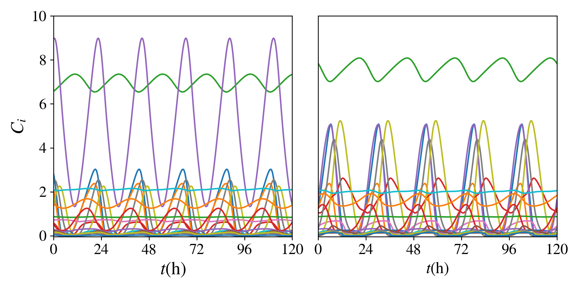
Figure 2: Timeseries of steady state oscillations of the (left) unforced system with natural period $T_{0}=22.04\mathrm{h}$, and (right) forced system with $T_{f}=24\mathrm{h}$. $C_{i}$ denotes the concentration of chemical species, $i$.

IV Results

IV.1 Single Neuron studies

When all neurons in a connected network are homogeneous, the network can in principle behave as each one of its individual neurons. We, therefore, begin our analysis by studying the behavior of a single circadian neuron.

As can be seen from Fig.2, in the absence of a photic stimulus, the circadian neuron will oscillate with its intrinsic frequency, while, in the presence of a photic stimulus, the neuron can get entrained. Notice that at the frequency locked “periodic steady state”, all the chemical species’ concentrations (normalized by $1\mathrm{nM}$ for simplicity) will oscillate with the same frequency but will not necessarily be at the same phase (e.g. not all species reach their maximum concentration simultaneously).

To explore entrained periodic solutions of a single circadian neuron, we perform pseudo-arclength continuation w.r.t the forcing angular frequency $\omega_{f}$ (reminder: $\omega_{f}=\frac{2\pi}{T_{f}}$), resulting in bifurcation diagrams like the one in Fig.3.

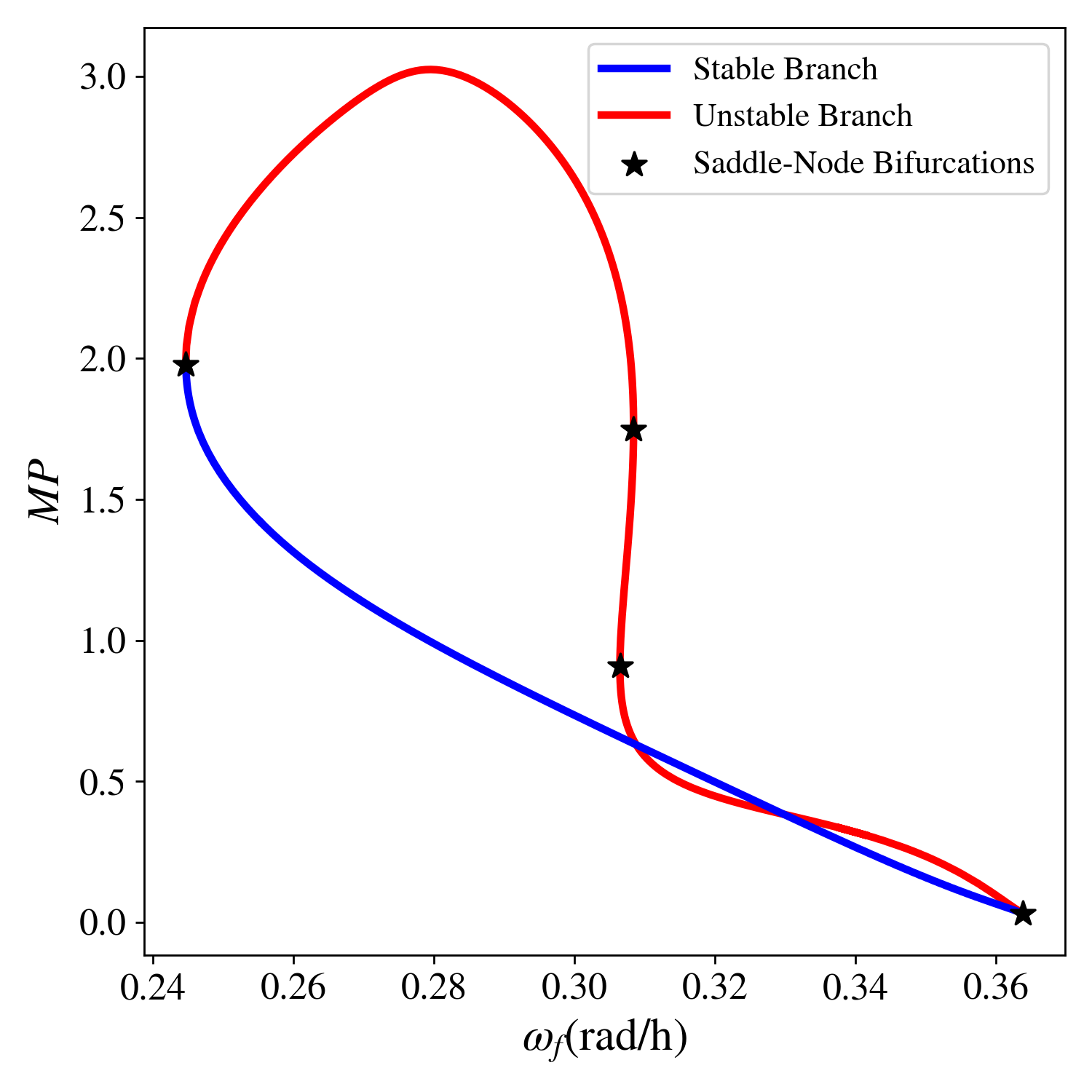
Figure 3: Bifurcation diagram for periodic steady states under photic stimulus for one circadian neuron. Here, the MP (Per mRNA) projection is shown. For reference: $\omega_{f}=0.262\mathrm{rad/h}$ for $T_{f}=24h$.

In bifurcation studies of entrainment problems, such loops are common when continuing solutions w.r.t. the forcing angular frequency Tomita and Kai (1979) and are termed isolas. Each point of the isola corresponds to a fixed point of the stroboscopic map, or, equivalently, to a periodic steady state of the original 21-dimensional ODE system. The limiting values of the bifurcation diagram w.r.t. the forcing angular frequency define the limits of entrainment and constitute saddle-node bifurcations of limit cycles. That is why the periodic solutions exchange stability at these points (see Fig. 3). Along the unstable branch (red) two additional saddle-node bifurcations are observed, further destabilizing the (already unstable) entrained solution.

To simulate the effect of the drug Longdaysin, we investigate how the synchronization limits change for different values of $k_{1}$ (normalized by $1\mathrm{h^{-1}}$ for simplicity). As suggested in St. John et al. (2014) we expect decreasing values of $k_{1}$, (which correspond to higher doses of Longdaysin) to lead to longer intrinsic (unforced) periods and larger oscillation amplitudes for the non-driven neurons. First, we perform continuation of the unforced system w.r.t. $k_{1}$ and examine the limit cycles at the two extreme limits of the $k_{1}$ interval (Fig.4). Then, we select a discrete, representative set of $k_{1}$ values, and calculate the limits of entrainment for each one of these values by constructing isolas (as in Fig. 3) with respect to the forcing frequency. Note that the nominal value of $k_{1}$ according to Vasalou, Herzog, and Henson (2011) is $k_{1}=0.49$ (also included).

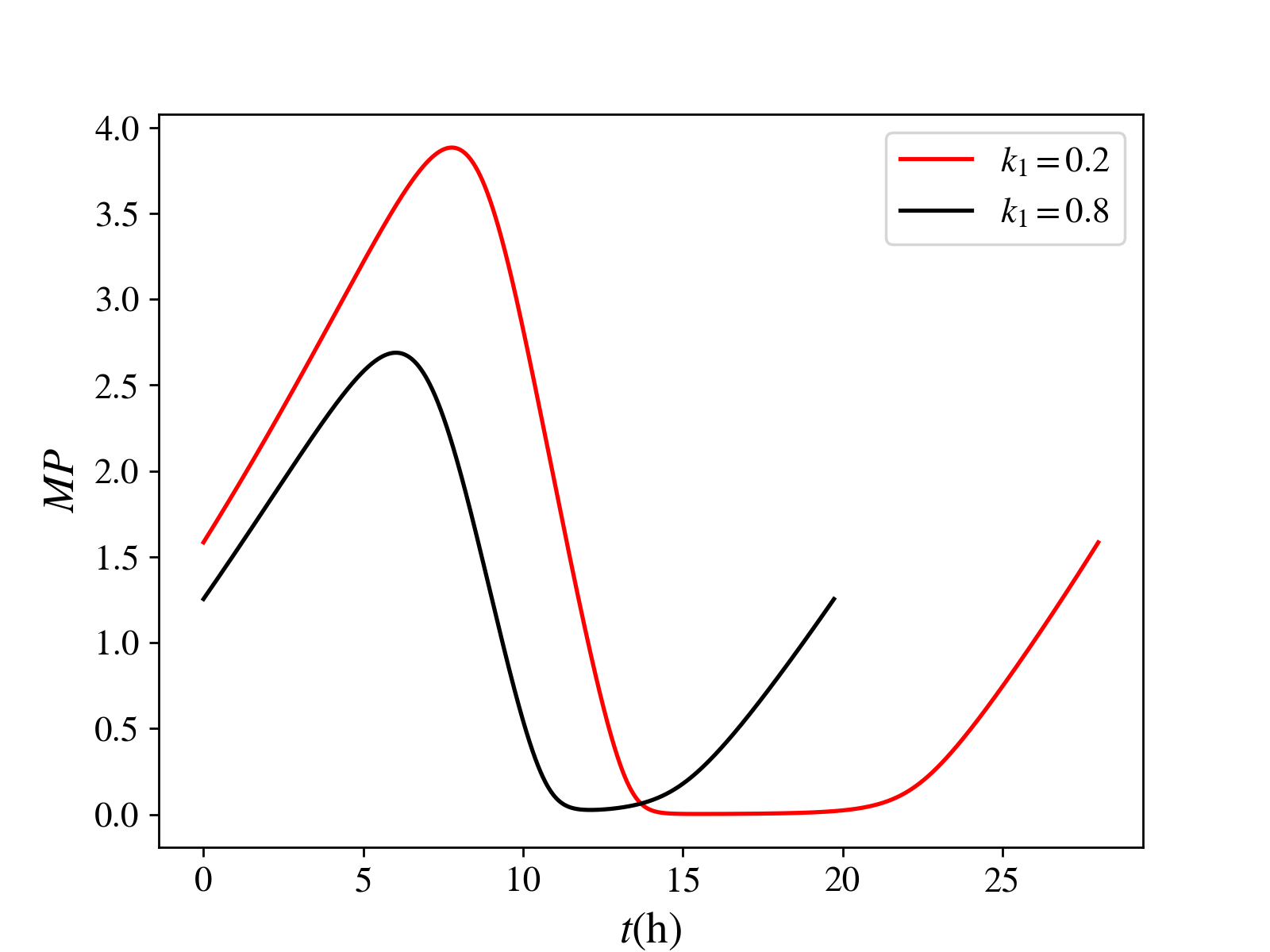
Figure 4: Unforced MP oscillations at the periodic steady state of $k_{1}=0.2$ and $k_{1}=0.8$.

We thus confirm that lower values of $k_{1}$ correspond to higher circadian periods and amplitudes of MP oscillations. It can also be seen from Fig.5 that lower values of $k_{1}$ result in tighter entrainment regions. The “natural” period of unforced oscillations always lies within the respective entrainment boundaries, as discussed in Tomita and Kai (1979). The bifurcation diagram in the $k_{1}-\omega_{f}$ space is equivalent to what is known in the literature as a resonance horn or Arnold tongue, and demarcates the parameter subregion where entrainment by an external forcing signal is feasible.

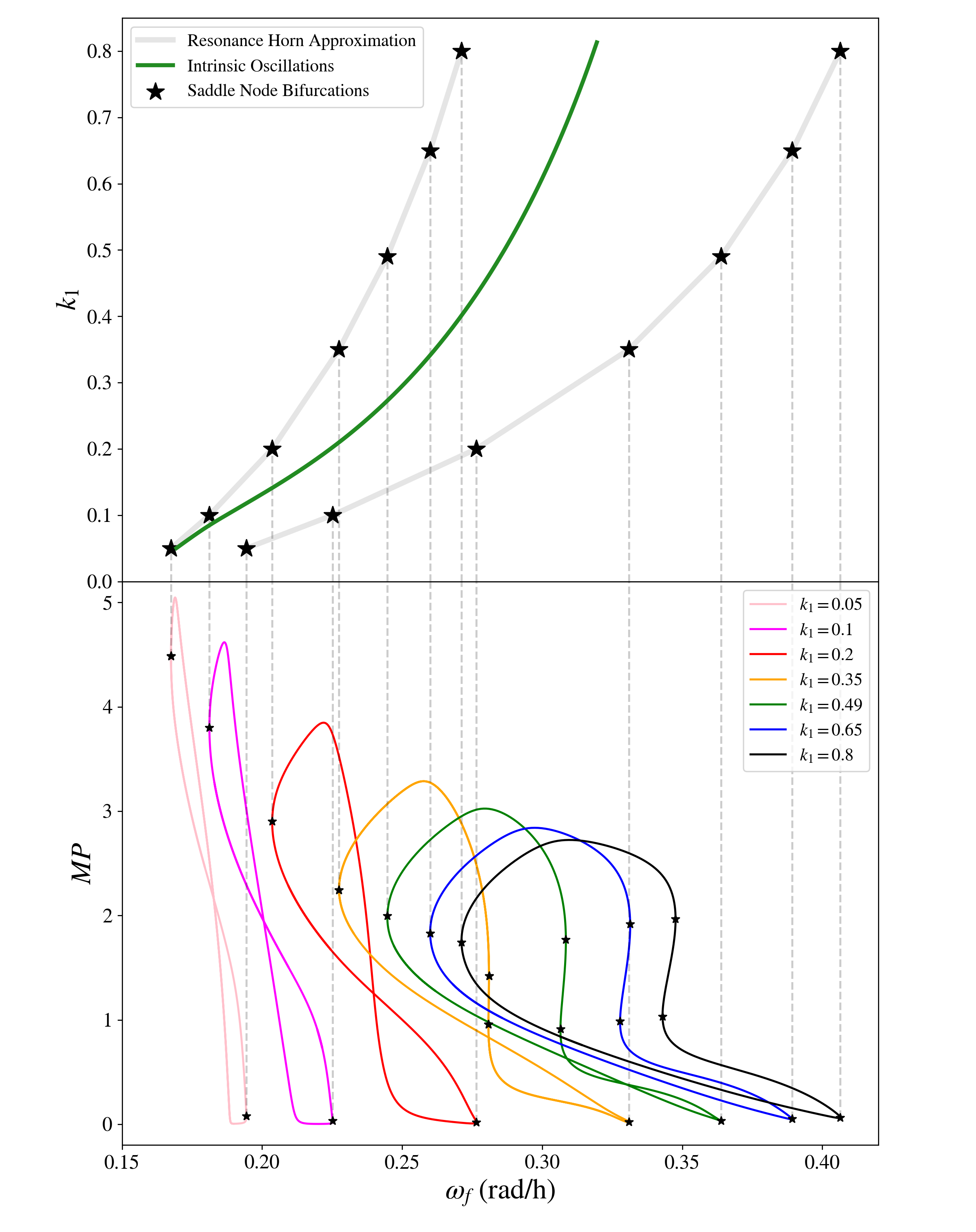
Figure 5: Bifurcation diagram for periodic steady states under photic stimulus for varying angular frequency $\omega_{f}$ and Longdaysin effect ($k_{1}$ value) in the case of a single circadian neuron. At the bottom subfigure, a collection of isolas is shown for discrete values of $k_{1}$. At the top figure, the resonance horn is approximated in the $\omega_{f}-k_{1}$ space.

Outside of the resonance horn in the $k_{1}-\omega_{f}$ space, various other dynamic responses are expected, e.g. quasiperiodicity, frequency locking, or chaos Tomita and Kai (1979). Fig. 6 shows quasiperiodic response for low values of $k_{1}$, at $\omega_{f}=0.16746\mathrm{rad/h}$ right after crossing the left saddle-node bifurcation (at $\omega_{f}=0.16749\mathrm{rad/h}$). Indeed, as it can be seen in the right panel of Fig. 6 the trajectories are now attracted to a high-dimensional torus.

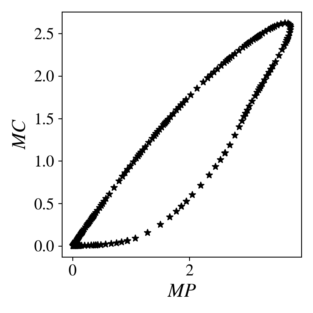
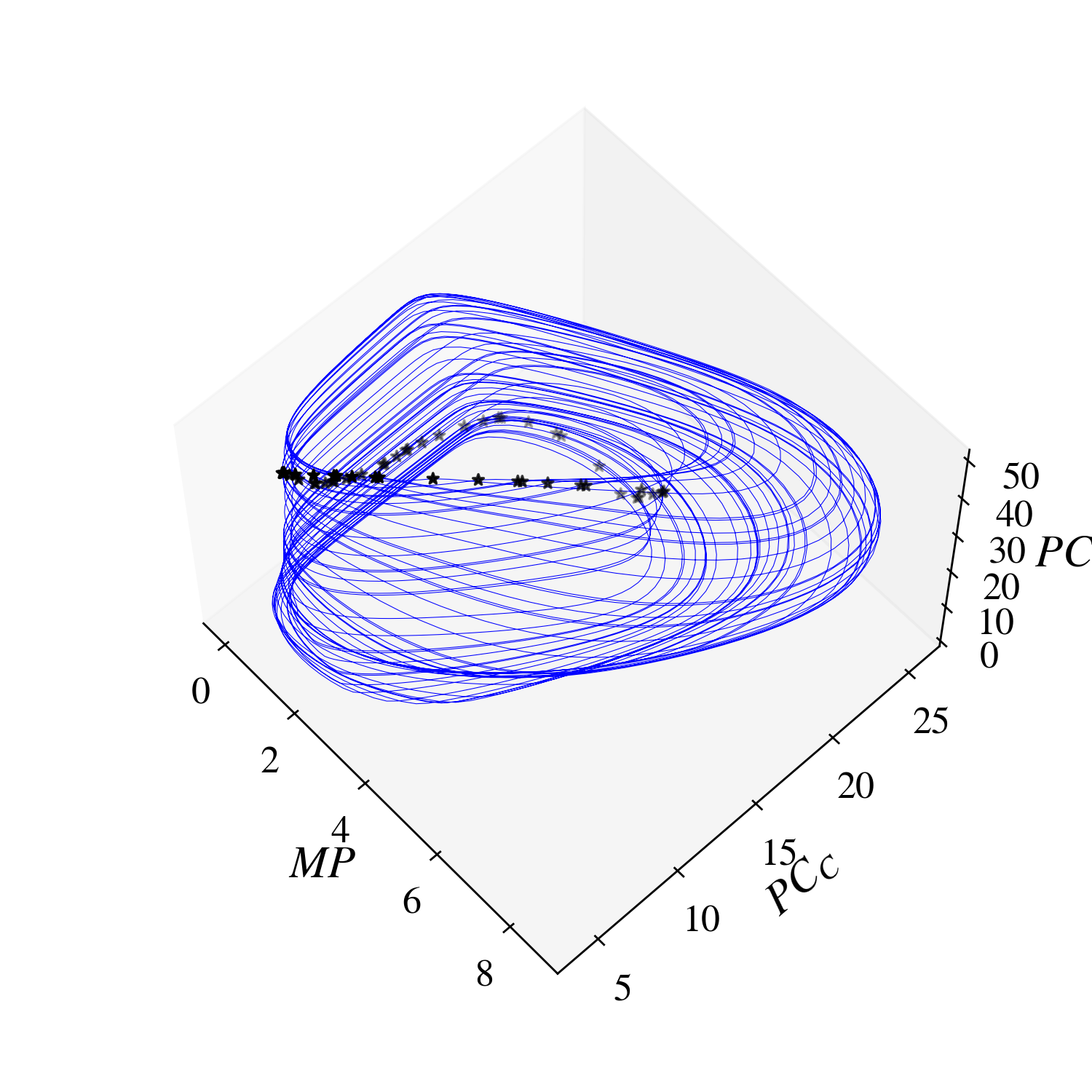
Figure 6: Loss of entrainment for $k_{1}=0.05,\omega_{f}=0.16746\mathrm{rad/h}$. Near the tip of the resonance horn (low $k_{1}$), quasiperiodicity is observed outside, but close to the entrainment limits. This can be confirmed by plotting iterates of the stroboscopic map (here, shown in the $MC-MP$ projection), where an invariant circle is observed (left). In the phase portrait representation (right), trajectories are attracted to a torus (here, the $MP-PC_{C}-PC$ projection is shown, along with stroboscopic map iterates). Note that $MP$: Per mRNA, $MB$: Bmal1 mRNA, $MC$: Cry mRNA, $PC$: nonphosphorylated Cry protein in the cytosol, $PC_{C}$: nonphosphorylated Per-Cry protein complex in the cytosol.

For higher $k_{1}$ values it is expected that different phenomena arise Kevrekidis, Schmidt, and Aris (1986); Tomita and Kai (1979). Indeed, for $k_{1}=0.49$ and $\omega_{f}=0.2446\mathrm{rad/h}$ a period-6 solution arises (frequency locking) after crossing the left bifurcation at $\omega_{f}=0.2447\mathrm{rad/h}$ (left panel, Fig. 7). Crossing the other limit of entrainment for $k_{1}=0.49$ (saddle-node bifurcation at $\omega_{f}=0.3638\mathrm{rad/h}$), chaos is observed to emerge for $\omega_{f}=0.3639\mathrm{rad/h}$ (right panel, Fig. 7).

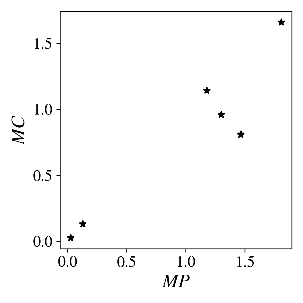
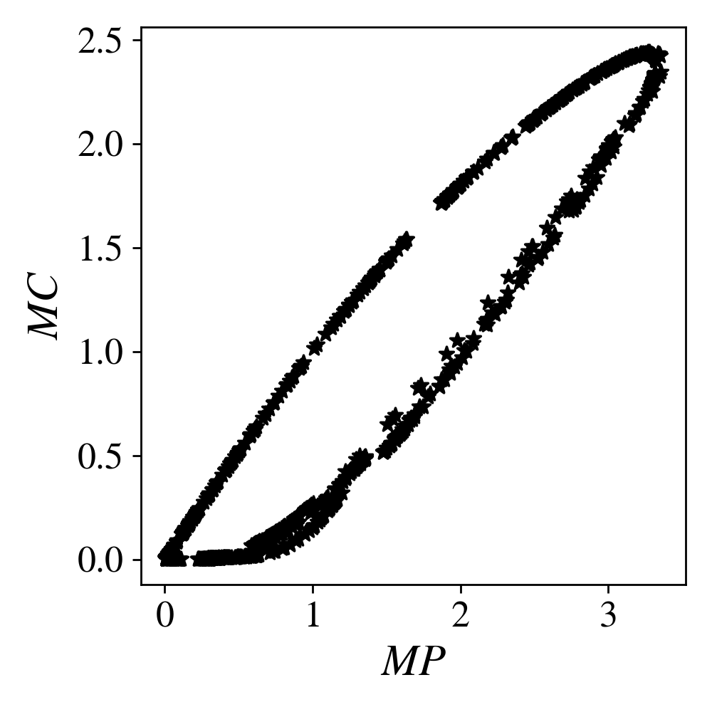
Figure 7: Loss of entrainment for $k_{1}=0.49:\omega_{f}=0.2446\mathrm{rad/h}$. (left panel) $\omega_{f}=0.3639\mathrm{rad/h}$ (right panel). Stroboscopic map iterates reveal frequency-locking and chaos respectively (here in the $MC-MP$ projection)

Figs.6, 7 stand as evidence that periodically forced circadian neurons demonstrate the entire gamut of dynamic responses typical of periodically forced dynamical systems Tomita and Kai (1979).

Subsequently, we perform continuaton of the periodic steady states w.r.t the duty cycle ($\phi$) for a fixed period (here, $T_{f}=24h$ or, equivalently, $\omega_{f}=0.268\mathrm{rad/h}$). In other words, we investigate entrainment of circadian neurons when the ratio of the length of the day (and, correspondingly, the duration of the night) changes.

As seen in Fig.8 there are entrainment limits w.r.t to the duty cycle as well. As anticipated, circadian neurons are unable to synchronize when the day/night phases become highly unbalanced. However, entrainment is not always lost in exactly the same way as the typical isolas we have encountered thus far.

For high day/night phase ratios, a saddle-node bifurcation marks the upper boundary of entrainment; but at low day/night ratios, the system undergoes a period doubling bifurcation (both the stable and the unstable branch). This means that the circadian neurons will return to the same state after two forcing periods. Interestingly, for some region, stable period-1 and period-2 solutions coexist, which means that circadian neurons are briefly bi-stable (Fig.9(a)). It is worth noting that the period-2 branches undergo an additional period-doubling bifurcation, leading to period-4 solutions. We hypothesize that this is the beginning of a period-doubling route to chaos (Fig. 9(b)) through a cascade of period-doubling bifurcations.

Note that integration of the ODEs describing neuronal dynamics of a single neuron was performed in Python’s solve_ivp platform, using the default RK23 integrator (Explicit Runge-Kutta method of order 3(2) Bogacki and Shampine (1989)), with absolute and relative tolerance at $10^{-8}$. Results where confirmed against MATLAB using the ode23 solver with relative tolerance at $10^{-7}$. Newton-Krylov GMRES was performed with our Python own code with tolerance $10^{-5}$, implemented as in Kelley, Kevrekidis, and Qiao (2004). Pseudo-arclength continuation was performed with our own Python code similarly to Doedel, Keller, and Kernevez (1991a), with an adaptive step, $\delta s$ (in the range $10^{-3}-10^{-1}$). The numerics for the neuronal network, results of which are presented in Section IV.2 are in similar ranges.

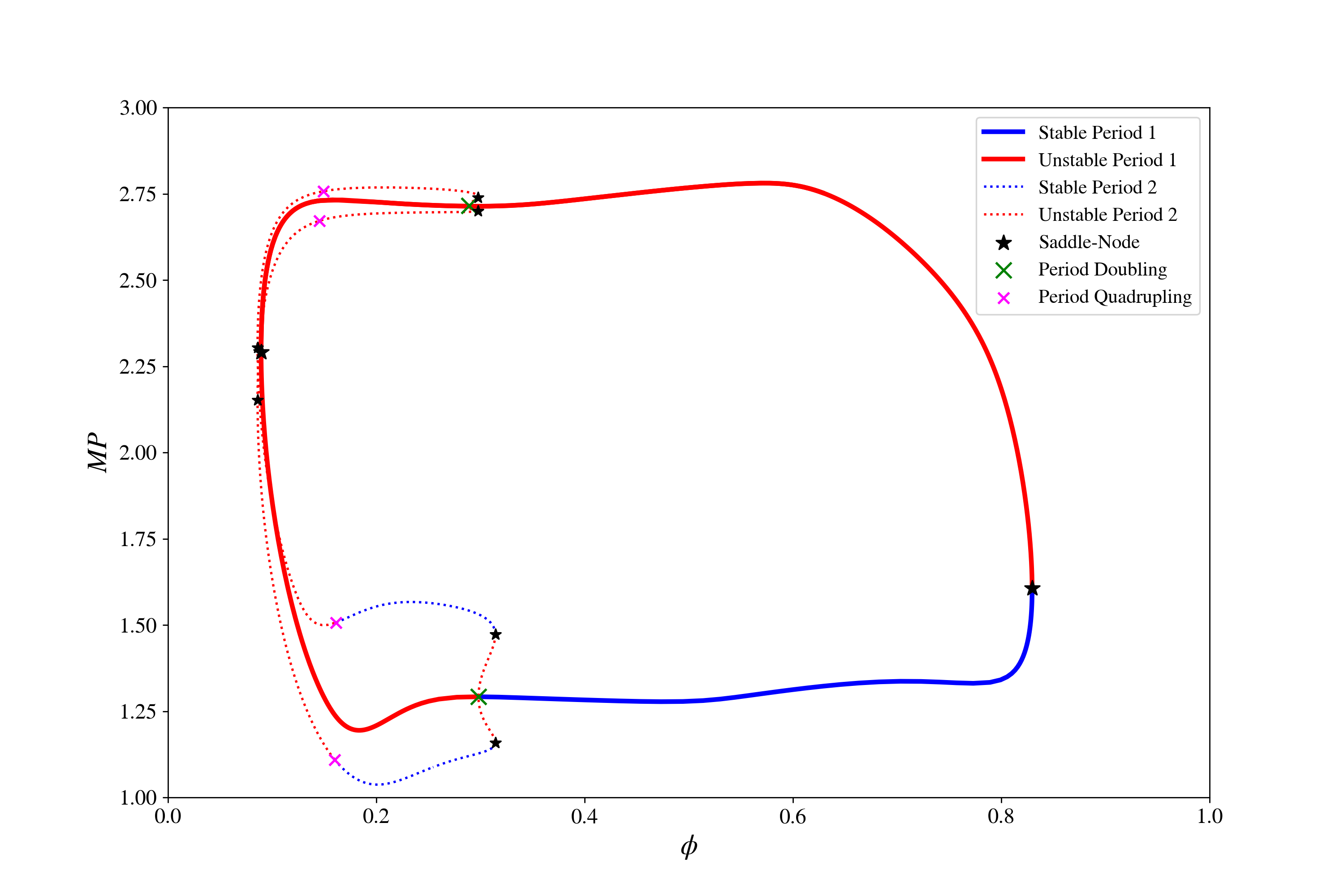
Figure 8: Bifurcation diagram for periodic steady states w.r.t the duty cycle $\phi$ under photic stimulus of fixed angular frequency $\omega_{f}=0.268\mathrm{rad/h}$ and without drug intervention ($k_{1}=0.49$) in the case of a single circadian neuron. Notice the additional bifurcations (leading to complex dynamics) towards lower day/night ratios.

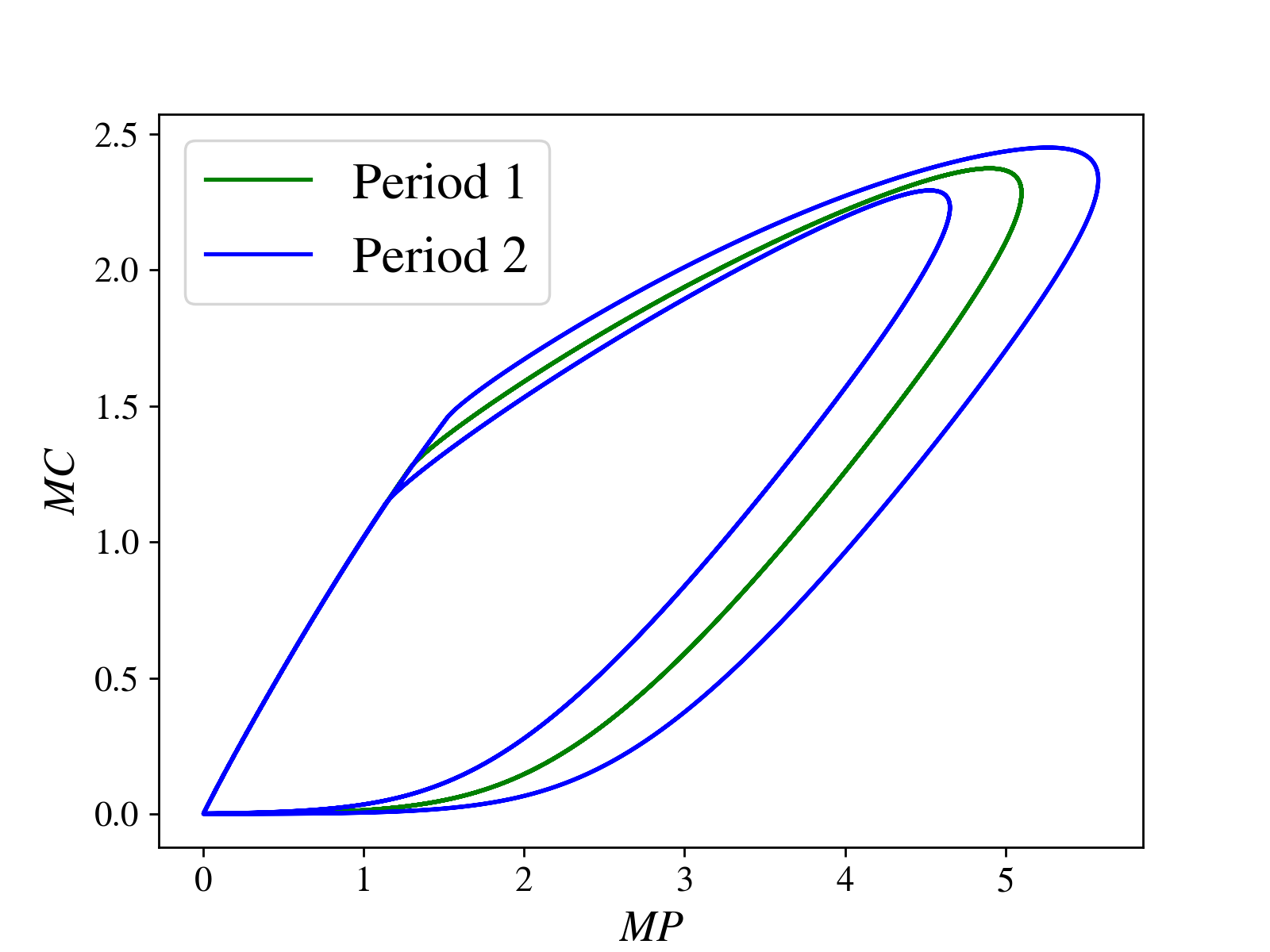
(a) $\phi=0.305$

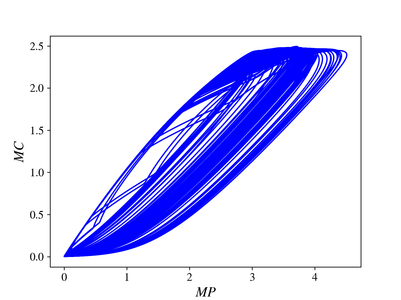
(b) $\phi=0.085$

Figure 9: Phase portraits at low $\phi$ values where bistability as well as chaos is observed.

IV.2 Heterogeneity in the Neuronal Network

In a realistic neuronal network each neuron is expected to be unique, or, in terms of computational modeling, to have its own intrinsic parameter values. As described in Section II, here we consider networks of 425 neurons that are heterogeneous w.r.t. the values of the parameter $v_{sP_{0}}$, for each neuron.

The effect of heterogeneity can be seen when plotting projections of the (now, $8925-$dimensional) limit cycle for two variables of each neuron (Fig. 11). We plot these limit cycles for two extents of heterogeneity (variance of the -here, normal- distribution of the heterogeneous parameter) and for five different simulated Longdaysin effects ($k_{1}$). As seen in Figs. 11 and 12 increasing heterogeneity causes the trajectories of different neurons to move further apart. However, all neurons follow qualitatively similar trajectories since the neuronal network is entrained.

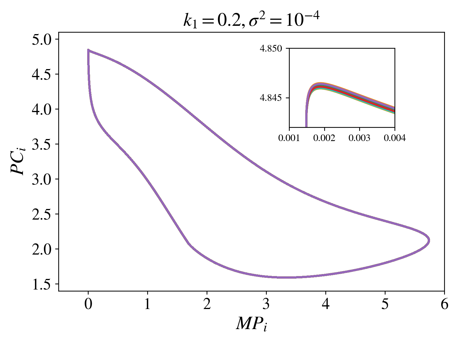
(a)

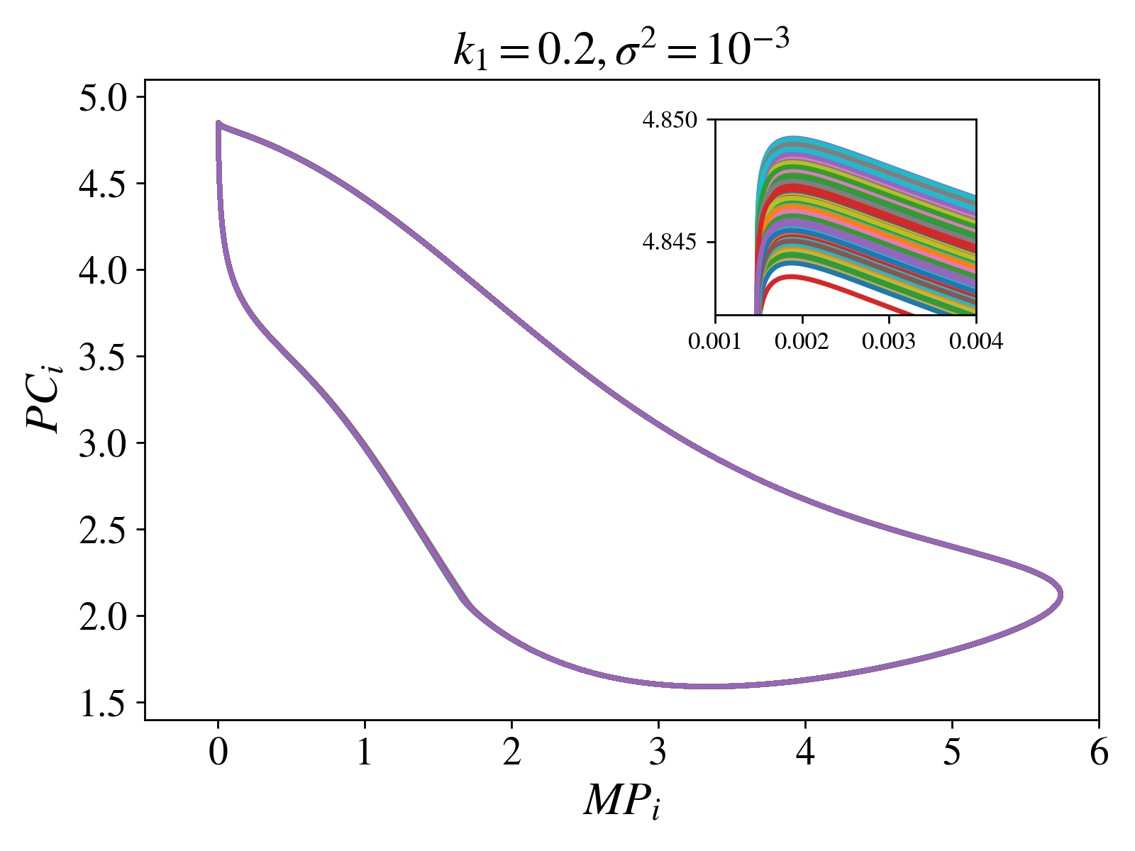
(b)

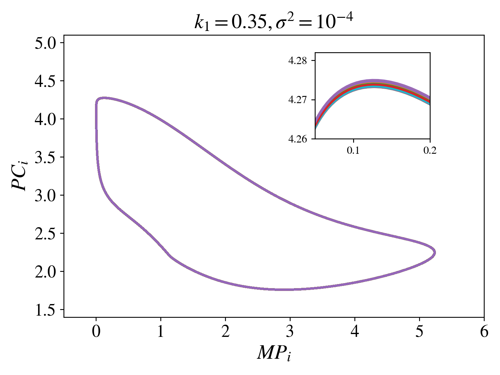
(c)

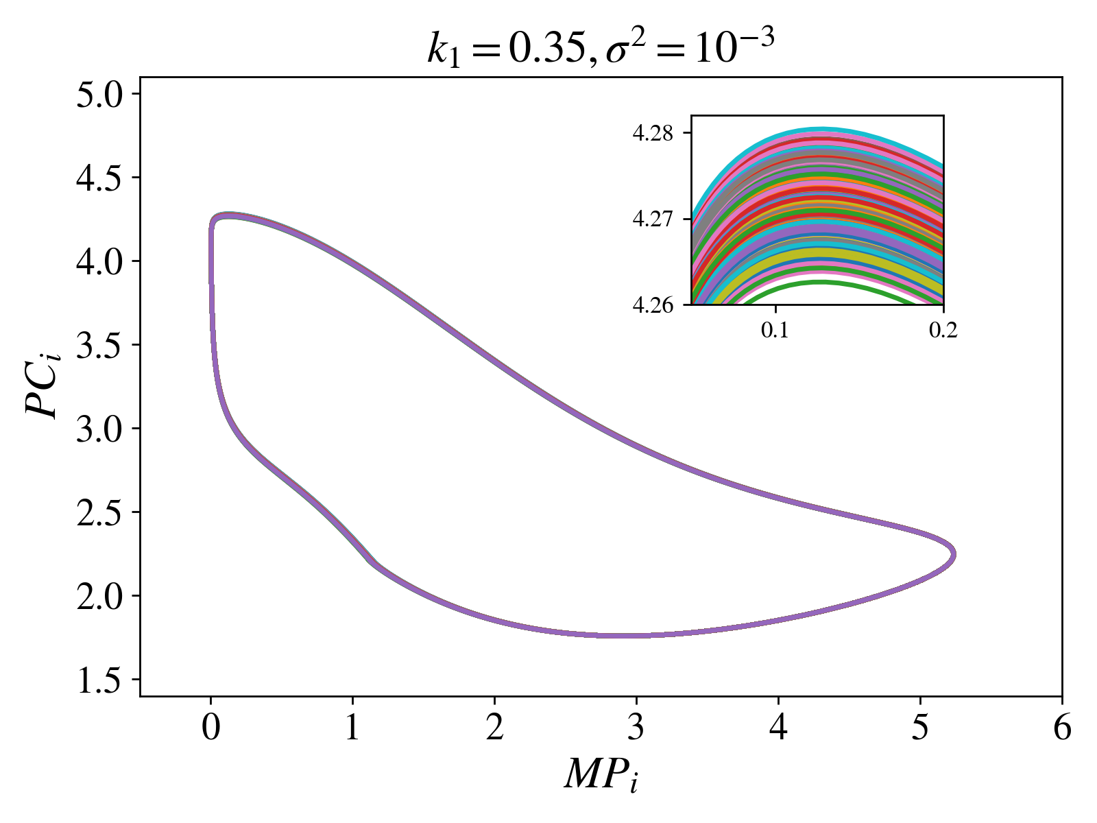
(d)

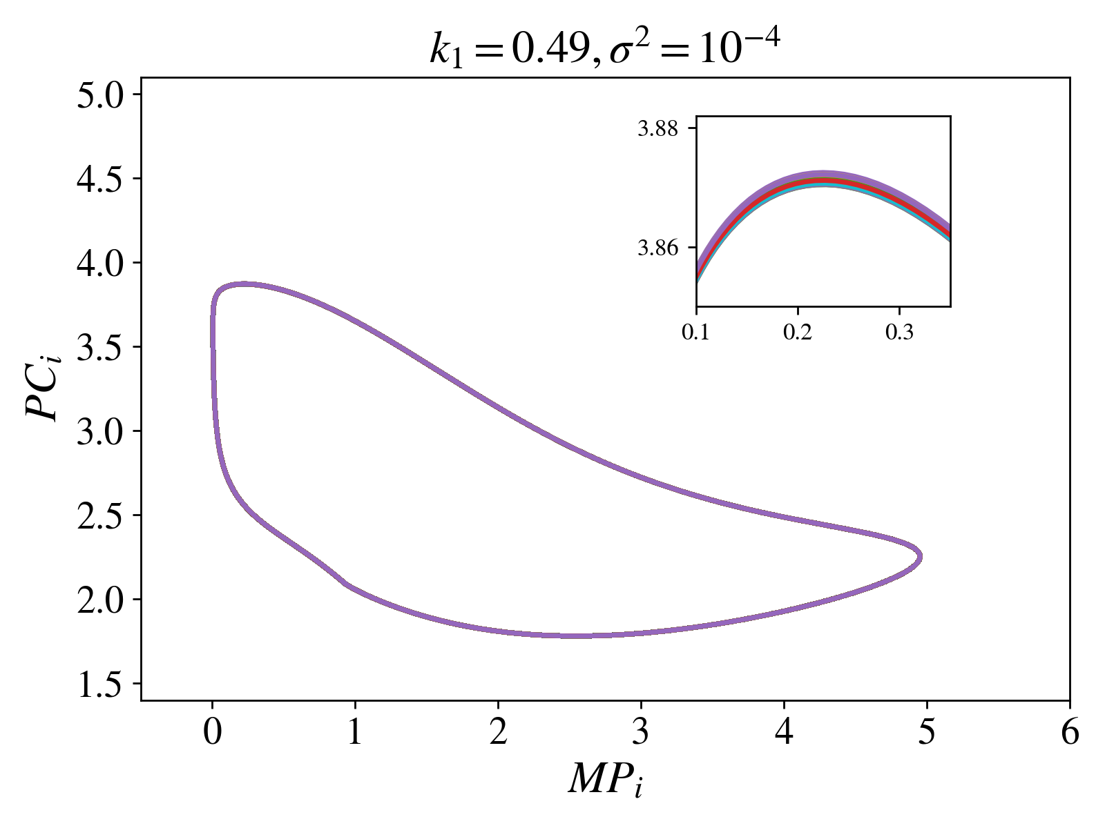
(e)

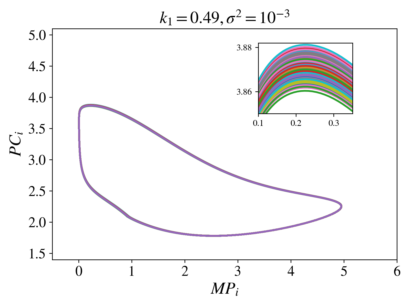
(f)

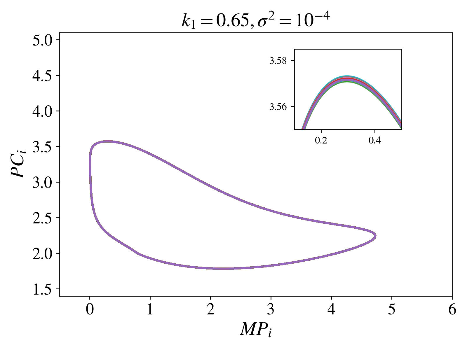
(a)

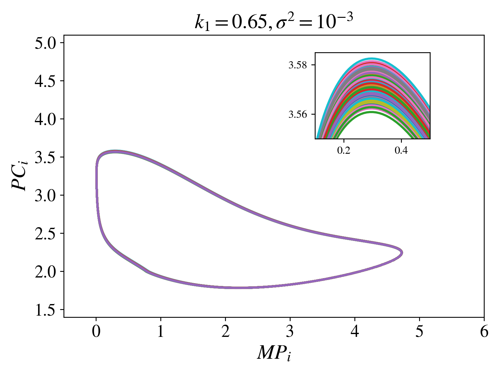
(b)

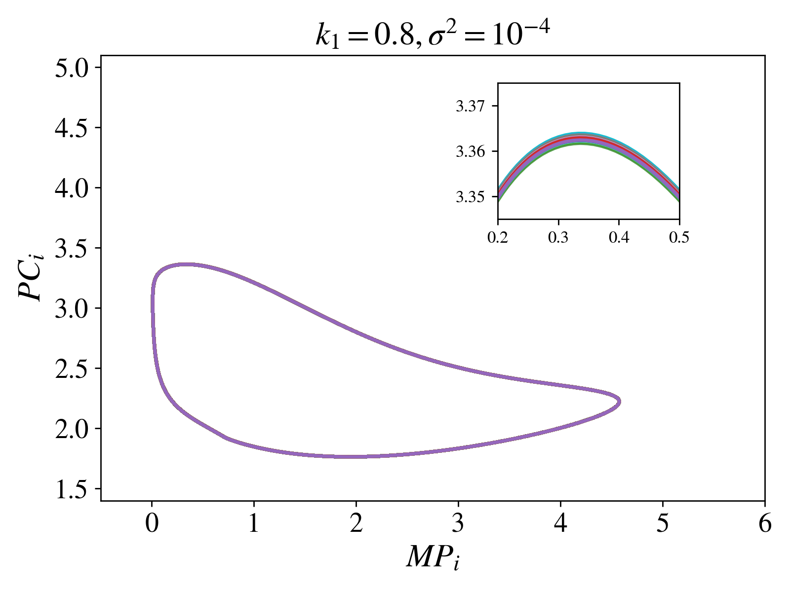
(c)

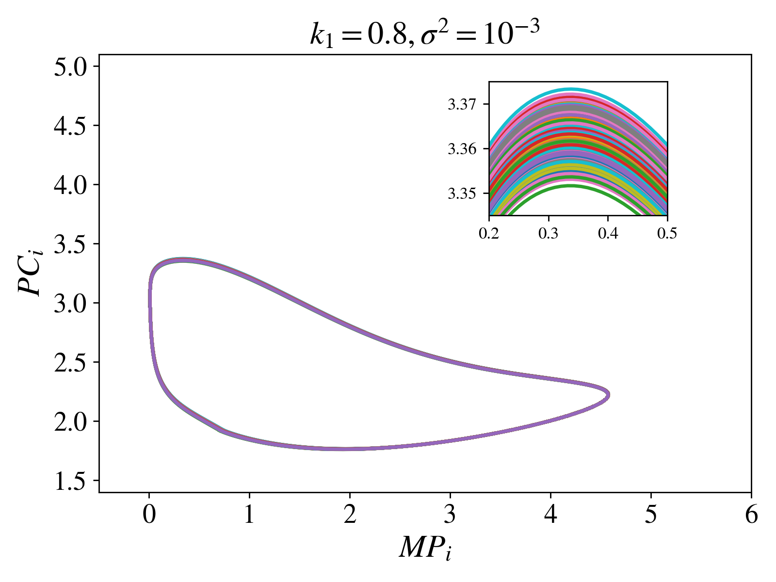
(d)

Figure 11: 2D projections of the $8925-$dimensional limit cycles ($i=1,...,8925)$), for $k_{1}$ in $\{0.2,0.35,0.49$ (nominal value)$,0.65,0.8\}$, for heterogeneity variance $10^{-3}$ or $10^{-4}$, with forcing angular frequency equal to the intrinsic one (for each $k_{1}$) and for $\phi=0.5$. Here the variables $PC_{i}$ and $MP_{i}$ are reported for every neuron, $i$.

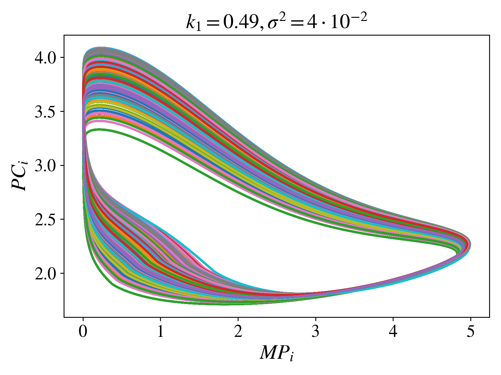
Figure 12: 2D projections of the $8925-$dimensional limit cycle for an even higher value of heterogeneity variance studied here ($\sigma^{2}=4\cdot 10^{-2}$), for comparison purposes. Here the variables $PC_{i}$ and $MP_{i}$ are reported for every neuron, $i$. This limit cycle was calculated for $k_{1}=0.49,\phi=0.5$ with forcing period $T_{f}=24\mathrm{h}$. This figure should be qualitatively compared to Figs. 10(e), 10(f).

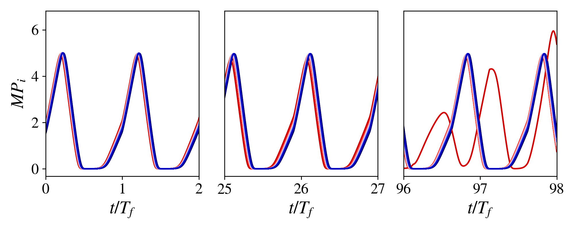
Figure 13: Loss of entrainment due to the emergence of a single “rogue” oscillator. Three panels show oscillation “snapshots” along a long trajectory. Initially (left panel), all neurons seem to be oscillating in synchrony. After some time (middle panel), the trajectory of one neuron slowly diverges from the rest, and for longer times (right panel) it starts oscillating erratically. Variable $MP_{i}$ is reported for every neuron $i$, while each neuron is colored by its heterogeneity $v_{sP_{0}}$ value; the rogue oscillator has the highest. Forcing parameters and heterogeneity variance value are mentioned in the text.

By analogy with Fig.5, we can computationally construct a resonance horn for each heterogeneity extent (Fig. 14). The entrainment limits do not change much with increasing neuron heterogeneity. This would seem to suggest robustness of the neuronal network to heterogeneity variations Komin et al. (2011).

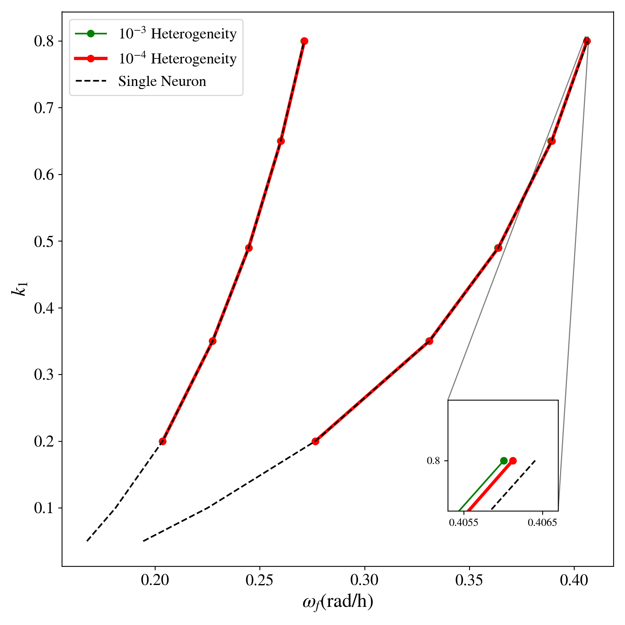
Figure 14: Superimposed resonance horns for the case of a single circadian neuron, and neuronal networks with varying extents of heterogeneity.

As in the case of single neuron studies, we can explore how entrainment is lost in the neuronal network. As can be seen in Fig. 13, after crossing the right saddle-node bifurcation for ($k_{1}=0.49$ and $\sigma^{2}=10^{-2},\omega_{f}=0.2455\mathrm{rad/h}$) a single “rogue” oscillator emerges. By that, we mean that even though most neurons appear to oscillate in synchrony, one of them gradually desynchronizes and starts oscillating “on its own” with varying amplitude. The emergence of such a “rogue” oscillator can be attributed to large variance of the heterogeneity parameter and is associated with bifurcations of the autonomous dynamical system Bold et al. (2007). In the dynamical systems literature a simple caricature of such a bifurcation is provided by the SNIPER (saddle-node infinite period) bifurcation Bertalan et al. (2017); Moon and Kevrekidis (2006).

Similarly to Fig.8 we can also continue periodic solutions of the high dimensional, heterogeneous neuronal network w.r.t. $\phi$, the day/night ratio (Fig.15). As expected, the bifurcation diagram for a single circadian neuron is again qualitatively similar to the large, mildly heterogeneous network diagram.

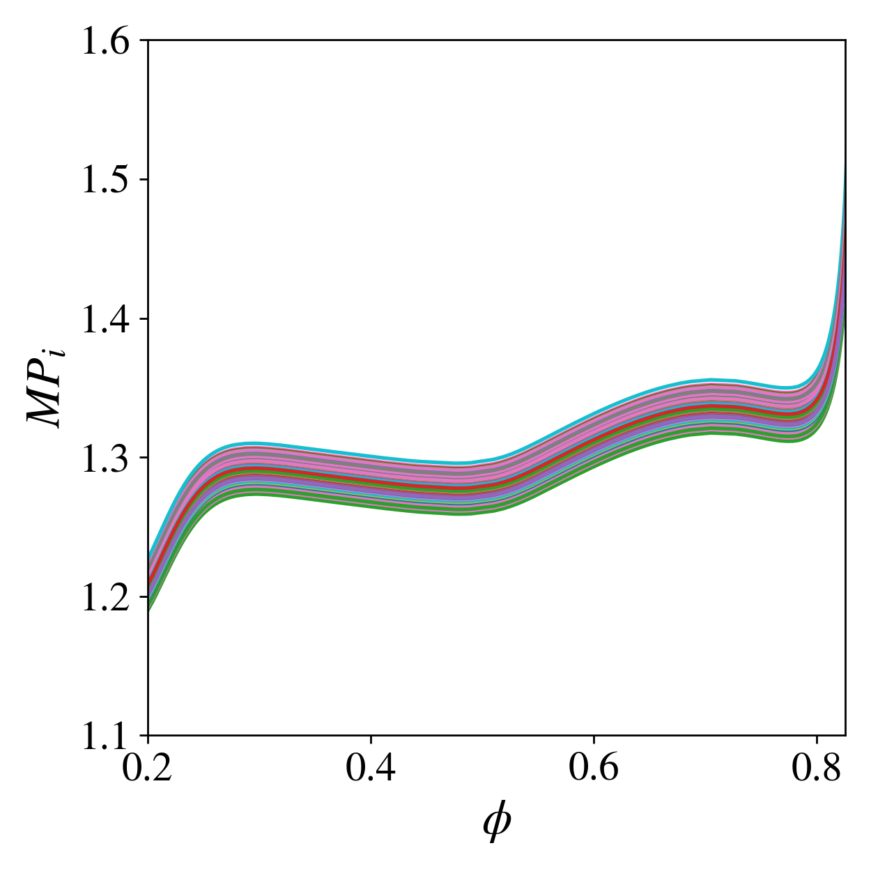
Figure 15: Continuation branch of periodic steady states solutions for the neuronal network w.r.t. the duty cycle $\phi$ for heterogeneity variance of value $\sigma^{2}=10^{-3}$ and $k_{1}=0.49,T_{f}=24h$. Here the variable $MP_{i}$ is reported for every neuron $i$ at the initial phase of the forcing. This should be compared to the lower branch in Fig. 8.

IV.3 A Data-Driven Embedding Space for Neuronal Heterogeneity.

Realistic neuronal networks are characterized by heterogeneity with respect to multiple physical properties. Enumeration and identification of such heterogeneities (and respective parameters for a computational model) from observed neuronal oscillation data is highly nontrivial, and is clearly affected by: (a) the quality and quantity of data; (b) stochasticity/noise inherent to measurements of biological systems; and (c) the complexity of the computational model and assumptions used in its formulation.

With increasing model complexity, it is clear that increasing parameter heterogeneity and variability (both for intrinsic kinetic parameters, and for structural network connectivity parameters) becomes important. When these parameters are not explicitly known, it is the variability of the neuronal behavior itself that encodes it; and so one can obtain a sense of the parameter heterogeneity from the neuronal time-series variability itself. In other words, it should be possible to infer the effective parametric heterogeneity/variability of the entire network by the richness of the variability of the observed oscillations of individual neurons. Here, we employ a data-driven approach to uncover an effective heterogeneity space purely from observed oscillation data. The algorithm we employ is Diffusion Maps (a nonlinear, manifold learning technique), to embed oscillation data in an effective, data-driven heterogeneity space Coifman and Lafon (2006); Thiem et al. (2021); Kemeth et al. (2018). The idea of creating such data-driven emergent spaces purely from observations was proposed in Kemeth et al. (2018, 2022) and it was used in the simple case of Kuramoto-type oscillators in Thiem et al. (2021).

As in Kemeth et al. (2018) we select data from a single phase of the limit cycle (the exact phase does not matter); the dataset therefore consists of 425 data points (number of neurons) in a 21-dimensional space (number of variables per neuron). As shown in Fig.16 diffusion maps reveals that the (synchronized) neuronal states are effectively one-dimensional, as $\psi_{1}$ seems to be the only independent eigenvector. The right panel of Fig.16 confirms that the observed data-based emergent heterogeneity descriptor $\psi_{1}$ in indeed one-to-one with the (true) intrinsic heterogeneity $v_{sP_{0}}$: the data-driven heterogeneity parametrization is one-to-one with the true physical one.

V Conclusions

This work was aimed at computationally exploring the limits of entrainment of circadian neurons and circadian neuronal networks. We employ modern techniques from scientific computing, such as matrix-free time-stepper based algorithms, to circumvent limitations inherent in high-dimensional dynamical systems. These algorithms enable the exploration of the simulated effect of (i) forcing frequency, (ii) forcing duty cycle, (iii) Longdaysin dosing level, and (iv) neuronal heterogeneity, on the ability of circadian neurons to entrain to the day/night cycle. Lastly, an unsupervised learning algorithm is used to discover an effective neuronal heterogeneity space from observed oscillation data.

A wealth of responses to different day/night cycle conditions is demonstrated, such as entrainment, quasiperiodicity, phase-locking and chaos. Linking fundamental concepts of nonlinear dynamics to computational neuroscience can lead to a holistic understanding of circadian dynamics and motivate real world applications. Especially in the case of simulated pharmacological effects, such a model can be thought as a computational “sandbox” for therapeutic (possibly, personalized) interventions to the SCN. Furthermore, combining scientific computing with machine learning can provide significant insights into the underlying degrees of freedom of systems as complex as the body’s own clock.

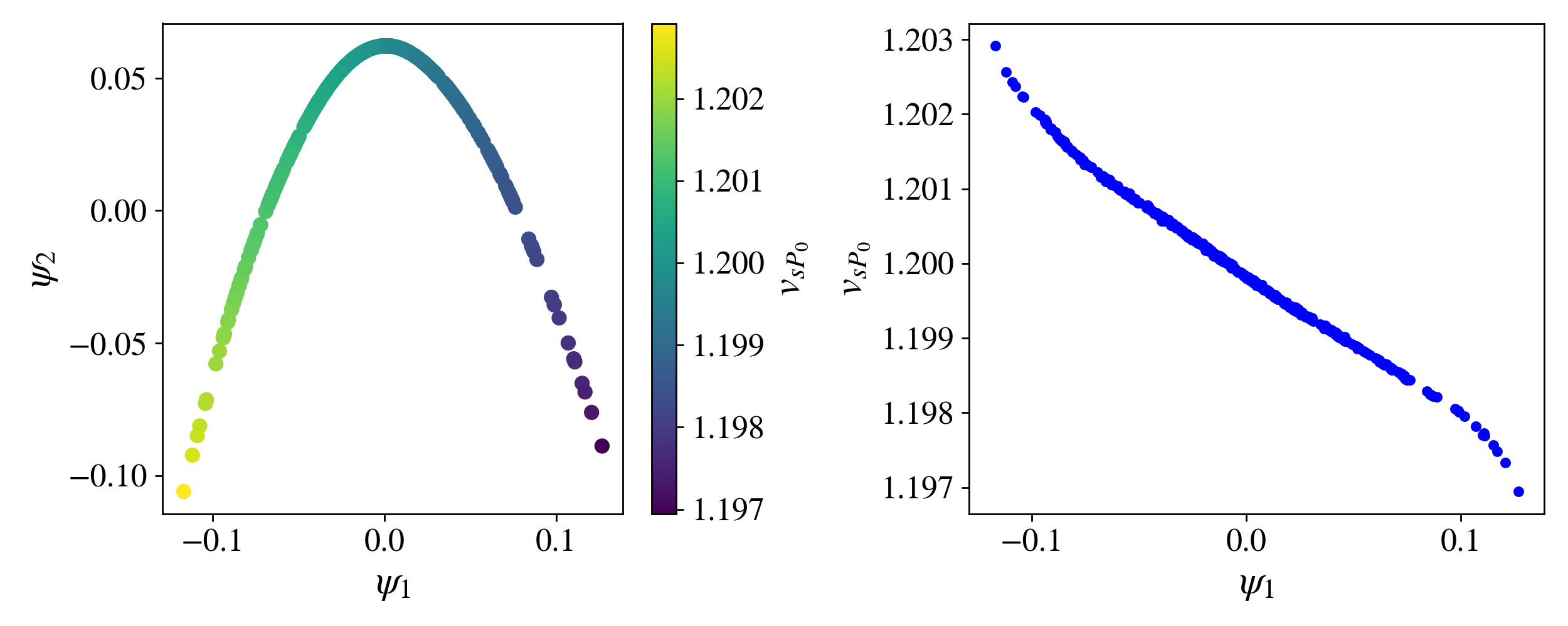
Figure 16: (left) Data from a single phase of the limit cycle plotted on the space defined by the first two nontrivial diffusion maps eigenvectors. All datapoints are colored by the a priori known heterogeneity parameter $v_{sP_{0}}$. Data are chosen from the case of $\phi=0.5,k_{1}=0.49,\sigma^{2}=10^{-3}$ for forcing angular velocity equal to the intrinsic one. (right) The first nontrivial diffusion maps eigenvector plotted against the heterogeneity parameter.

References

- Ma and Morrison (2022) M. A. Ma and E. H. Morrison, “Neuroanatomy, nucleus suprachiasmatic,” in StatPearls (StatPearls Publishing, Treasure Island (FL), 2022).
- Hastings, Maywood, and Brancaccio (2018) M. H. Hastings, E. S. Maywood, and M. Brancaccio, “Generation of circadian rhythms in the suprachiasmatic nucleus,” Nature Reviews Neuroscience 19, 453–469 (2018).
- Sack et al. (2007a) R. L. Sack, D. Auckley, R. R. Auger, M. A. Carskadon, K. P. Wright Jr., M. V. Vitiello, I. V. Zhdanova, and of Sleep Medicine American Academy, “Circadian rhythm sleep disorders: part i, basic principles, shift work and jet lag disorders. an american academy of sleep medicine review,” Sleep 30, 1460–1483 (2007a), 18041480[pmid].
- Sack et al. (2007b) R. L. Sack, D. Auckley, R. R. Auger, M. A. Carskadon, J. Wright, Kenneth P., M. V. Vitiello, and I. V. Zhdanova, “Circadian Rhythm Sleep Disorders: Part II, Advanced Sleep Phase Disorder, Delayed Sleep Phase Disorder, Free-Running Disorder, and Irregular Sleep-Wake Rhythm,” Sleep 30, 1484–1501 (2007b), https://academic.oup.com/sleep/article-pdf/30/11/1484/13663700/sleep-30-11-1484.pdf .
- Scheer et al. (2009) F. A. J. L. Scheer, M. F. Hilton, C. S. Mantzoros, and S. A. Shea, “Adverse metabolic and cardiovascular consequences of circadian misalignment,” Proceedings of the National Academy of Sciences of the United States of America 106, 4453–4458 (2009), 19255424[pmid].
- Nakano et al. (1991) S. Nakano, K. Uchida, T. Kigoshi, S. Azukizawa, R. Iwasaki, M. Kaneko, and S. Morimoto, “Circadian Rhythm of Blood Pressure in Normotensive NIDDM Subjects: Its Relationship to Microvascular Complications,” Diabetes Care 14, 707–711 (1991), https://diabetesjournals.org/care/article-pdf/14/8/707/341154/14-8-707.pdf .
- Savvidis and Koutsilieris (2012) C. Savvidis and M. Koutsilieris, “Circadian rhythm disruption in cancer biology,” Molecular Medicine 18, 1249–1260 (2012).
- Germain and Kupfer (2008) A. Germain and D. J. Kupfer, “Circadian rhythm disturbances in depression,” Human psychopharmacology 23, 571–585 (2008), 18680211[pmid].
- Vadnie and McClung (2017) C. A. Vadnie and C. A. McClung, “Circadian rhythm disturbances in mood disorders: Insights into the role of the suprachiasmatic nucleus,” Neural Plasticity 2017, 1504507 (2017).
- Turek and Losee-Olson (1986) F. W. Turek and S. Losee-Olson, “A benzodiazepine used in the treatment of insomnia phase-shifts the mammalian circadian clock,” Nature 321, 167–168 (1986).
- Sack et al. (2000) R. L. Sack, R. W. Brandes, A. R. Kendall, and A. J. Lewy, “Entrainment of free-running circadian rhythms by melatonin in blind people,” New England Journal of Medicine 343, 1070–1077 (2000), pMID: 11027741, https://doi.org/10.1056/NEJM200010123431503 .
- Huang et al. (2020) S. Huang, X. Jiao, D. Lu, X. Pei, D. Qi, and Z. Li, “Recent advances in modulators of circadian rhythms: an update and perspective,” Journal of Enzyme Inhibition and Medicinal Chemistry 35, 1267–1286 (2020), pMID: 32506972, https://doi.org/10.1080/14756366.2020.1772249 .
- St. John et al. (2014) P. C. St. John, T. Hirota, S. A. Kay, and F. J. Doyle, “Spatiotemporal separation of per and cry posttranslational regulation in the mammalian circadian clock,” Proceedings of the National Academy of Sciences 111, 2040–2045 (2014), https://www.pnas.org/content/111/5/2040.full.pdf .
- Hirota et al. (2012) T. Hirota, J. W. Lee, P. C. S. John, M. Sawa, K. Iwaisako, T. Noguchi, P. Y. Pongsawakul, T. Sonntag, D. K. Welsh, D. A. Brenner, F. J. Doyle, P. G. Schultz, and S. A. Kay, “Identification of small molecule activators of cryptochrome,” Science 337, 1094–1097 (2012), https://www.science.org/doi/pdf/10.1126/science.1223710 .
- Vasalou, Herzog, and Henson (2011) C. Vasalou, E. Herzog, and M. Henson, “Multicellular model for intercellular synchronization in circadian neural networks,” Biophysical Journal 101, 12–20 (2011).
- Vasalou and Henson (2011) C. Vasalou and M. A. Henson, “A multicellular model for differential regulation of circadian signals in the core and shell regions of the suprachiasmatic nucleus,” Journal of Theoretical Biology 288, 44–56 (2011).
- Leloup and Goldbeter (2003) J.-C. Leloup and A. Goldbeter, “Toward a detailed computational model for the mammalian circadian clock,” Proceedings of the National Academy of Sciences 100, 7051–7056 (2003), https://www.pnas.org/doi/pdf/10.1073/pnas.1132112100 .
- Leloup and Goldbeter (2004) J.-C. Leloup and A. Goldbeter, “Modeling the mammalian circadian clock: Sensitivity analysis and multiplicity of oscillatory mechanisms,” Journal of Theoretical Biology 230, 541–562 (2004), special Issue in honour of Arthur T. Winfree.
- To et al. (2007) T.-L. To, M. A. Henson, E. D. Herzog, and r. Doyle, Francis J, “A molecular model for intercellular synchronization in the mammalian circadian clock,” Biophysical journal 92, 3792–3803 (2007), 17369417[pmid].
- Vasalou and Henson (2010) C. Vasalou and M. A. Henson, “A multiscale model to investigate circadian rhythmicity of pacemaker neurons in the suprachiasmatic nucleus,” PLOS Computational Biology 6, 1–15 (2010).
- Henson (2013) M. Henson, “Multicellular models of intercellular synchronization in circadian neural networks,” Chaos, Solitons & Fractals 50, 48–64 (2013).
- Yamaguchi et al. (2003) S. Yamaguchi, H. Isejima, T. Matsuo, R. Okura, K. Yagita, M. Kobayashi, and H. Okamura, “Synchronization of cellular clocks in the suprachiasmatic nucleus,” Science 302, 1408–1412 (2003), https://www.science.org/doi/pdf/10.1126/science.1089287 .
- Kevrekidis, Schmidt, and Aris (1986) I. Kevrekidis, L. Schmidt, and R. Aris, “Some common features of periodically forced reacting systems,” Chemical Engineering Science 41, 1263–1276 (1986).
- Saad and Schultz (1986) Y. Saad and M. H. Schultz, “Gmres: A generalized minimal residual algorithm for solving nonsymmetric linear systems,” SIAM Journal on scientific and statistical computing 7, 856–869 (1986).
- Kelley, Kevrekidis, and Qiao (2004) C. T. Kelley, I. G. Kevrekidis, and L. Qiao, “Newton-krylov solvers for time-steppers,” (2004).
- Dickson et al. (2007) K. I. Dickson, C. T. Kelley, I. C. F. Ipsen, and I. G. Kevrekidis, “Condition estimates for pseudo-arclength continuation,” SIAM Journal on Numerical Analysis 45, 263–276 (2007), https://doi.org/10.1137/060654384 .
- Vandekerckhove, Kevrekidis, and Roose (2009) C. Vandekerckhove, I. Kevrekidis, and D. Roose, “An efficient newton-krylov implementation of the constrained runs scheme for initializing on a slow manifold,” Journal of Scientific Computing 39, 167–188 (2009).
- Kelley (2003) C. T. Kelley, Solving Nonlinear Equations with Newton’s Method (2003) pp. 57–83, https://epubs.siam.org/doi/pdf/10.1137/1.9780898718898.ch3 .
- Siettos, Pantelides, and Kevrekidis (2003) C. I. Siettos, C. C. Pantelides, and I. G. Kevrekidis, “Enabling dynamic process simulators to perform alternative tasks: A time-stepper-based toolkit for computer-aided analysis,” Industrial & Engineering Chemistry Research 42, 6795–6801 (2003), https://doi.org/10.1021/ie021062w .
- Arnoldi (1951) W. E. Arnoldi, “The principle of minimized iterations in the solution of the matrix eigenvalue problem,” Quarterly of Applied Mathematics 9, 17–29 (1951).
- Keller (1978) H. B. Keller, “Global homotopies and newton methods,” in Recent Advances in Numerical Analysis, edited by C. De Boor and G. H. Golub (Academic Press, 1978) pp. 73–94.
- Doedel, Keller, and Kernevez (1991a) E. Doedel, H. B. Keller, and J. P. Kernevez, “Numerical analysis and control of bifurcation problems (i): Bifurcation in finite dimensions,” International Journal of Bifurcation and Chaos 01, 493–520 (1991a), https://doi.org/10.1142/S0218127491000397 .
- Doedel, Keller, and Kernevez (1991b) E. Doedel, H. B. Keller, and J. P. Kernevez, “Numerical analysis and control of bifurcation problems (ii): Bifurcation in infinte dimensions,” International Journal of Bifurcation and Chaos 01, 745–772 (1991b), https://doi.org/10.1142/S0218127491000555 .
- Tomita and Kai (1979) K. Tomita and T. Kai, “Chaotic response of a limit cycle,” Journal of Statistical Physics 21, 65–86 (1979).
- Bogacki and Shampine (1989) P. Bogacki and L. Shampine, “A 3(2) pair of runge - kutta formulas,” Applied Mathematics Letters 2, 321–325 (1989).
- Komin et al. (2011) N. Komin, A. C. Murza, E. Hernández-García, and R. Toral, “Synchronization and entrainment of coupled circadian oscillators,” Interface Focus 1, 167–176 (2011).
- Bold et al. (2007) K. A. Bold, Y. Zou, I. G. Kevrekidis, and M. A. Henson, “An equation-free approach to analyzing heterogeneous cell population dynamics,” Journal of Mathematical Biology 55, 331–352 (2007).
- Bertalan et al. (2017) T. Bertalan, Y. Wu, C. Laing, C. W. Gear, and I. G. Kevrekidis, “Coarse-grained descriptions of dynamics for networks with both intrinsic and structural heterogeneities,” Frontiers in Computational Neuroscience 11 (2017), 10.3389/fncom.2017.00043.
- Moon and Kevrekidis (2006) S. J. Moon and I. G. Kevrekidis, “An equation-free approach to coupled oscillator dynamics: the kuramoto model example,” International Journal of Bifurcation and Chaos 16, 2043–2052 (2006).
- Coifman and Lafon (2006) R. R. Coifman and S. Lafon, “Diffusion maps,” Applied and Computational Harmonic Analysis 21, 5–30 (2006), special Issue: Diffusion Maps and Wavelets.
- Thiem et al. (2021) T. N. Thiem, F. P. Kemeth, T. Bertalan, C. R. Laing, and I. G. Kevrekidis, “Global and local reduced models for interacting, heterogeneous agents,” Chaos: An Interdisciplinary Journal of Nonlinear Science 31, 073139 (2021), https://doi.org/10.1063/5.0055840 .
- Kemeth et al. (2018) F. P. Kemeth, S. W. Haugland, F. Dietrich, T. Bertalan, K. Höhlein, Q. Li, E. M. Bollt, R. Talmon, K. Krischer, and I. G. Kevrekidis, “An emergent space for distributed data with hidden internal order through manifold learning,” IEEE access : practical innovations, open solutions 6, 77402–77413 (2018), 31179198[pmid].
- Kemeth et al. (2022) F. P. Kemeth, T. Bertalan, T. Thiem, F. Dietrich, S. J. Moon, C. R. Laing, and I. G. Kevrekidis, “Learning emergent partial differential equations in a learned emergent space,” Nature Communications 13, 3318 (2022).
- Lust and Roose (1998) K. Lust and D. Roose, “An adaptive newton–picard algorithm with subspace iteration for computing periodic solutions,” SIAM Journal on Scientific Computing 19, 1188–1209 (1998).