Quantum gravitational signatures in next-generation gravitational wave detectors

Abstract

A recent study established a correspondence between the Generalized Uncertainty Principle (GUP) and Modified theories of gravity, particularly Stelle gravity. We investigate the consequences of this correspondence for inflation and cosmological observables by evaluating the power spectrum of the scalar and tensor perturbations using two distinct methods. First, we employ PLANCK observations to determine the GUP parameter $\gamma_{0}$. Then, we use the value of $\gamma_{0}$ to investigate the implications of quantum gravity on the power spectrum of primordial gravitational waves and their possible detectability in the next-generation detectors, like Einstein Telescope and Cosmic explorer.

Since its discovery, the cosmic microwave background (CMB) has been an indispensable tool for understanding the very early universe. Consequently, observational cosmology has made incredible progress over the last three decades and thanks to the observation of temperature fluctuations at the last scattering surface, one has been able to identify the physical origins of the primordial density perturbations in the very early universe [1, 2, 3, 4, 5, 6, 7]. The inflationary paradigm provides a causal mechanism for the origin of these perturbations and the inflationary epoch magnifies the tiny fluctuations in the quantum fields present at the beginning of the epoch into classical perturbations that leave an imprint as anisotropies in the CMB [8, 9, 10, 11, 12, 13]. A key prediction of inflation is the generation of primordial gravitational waves (PGWs) [14, 15, 16].

Therefore, significant effort is currently underway to detect PGWs via B-mode polarization measurements of the CMB [17, 18, 19, 20, 21, 22, 5]. This is because B-modes of CMB are only sourced by the differential stretching of spacetime associated with the PGWs [16, 23]. However, the primordial B-mode polarization signal is weak and could be swamped inside dust emission in our galaxy [24, 20, 5]. Efforts are also underway to directly detect PGWs [25, 26, 27, 28, 29, 30]. In this work, we explicitly show that PGWs carry quantum gravitational signatures that can potentially be observed in the next-generation gravitational wave detectors such as the Einstein Telescope (ET) and Cosmic Explorer (CE).

Theories of Quantum Gravity (QG) predict the existence of a minimum measurable length and/or a maximum measurable momentum of particles [31, 32]. The experimental implications of this scale are explored in Quantum Gravity Phenomenology (QGP) [33]. This QGP/QG scale is most easily realized by deforming the standard Heisenberg uncertainty relation to the so-called Generalized Uncertainty Principle (GUP) [34, 35, 36, 37, 38, 39, 40, 41, 42, 43, 44, 45, 46, 47, 48, 49, 50, 51, 52, 53, 54, 55, 56, 57, 58, 59, 60, 61, 62, 63, 64, 65, 66, 67, 68, 69, 70, 71, 72, 73, 74, 75, 76, 77, 78, 79]. Recently, we proposed a Lorentz invariant implementation of GUP, wherein we modified the canonical commutation relation to [80]:

$$[x^{\mu},p^{\nu}]=i\hbar\eta^{\mu\nu}(1-\gamma p^{\sigma}p_{\sigma})-2i\hbar\gamma p^{\mu}p^{\nu},$$ (1)

where in natural units ($\hbar=c=1$),

$$\gamma=\gamma_{0}\,M_{\text{Planck}}^{-2}=\gamma_{0}\,l_{\text{Planck}}^{2},$$ (2)

is the Lorentz invariant scale, and $\gamma_{0}$ is a numerical parameter used to fix the scale . Experimental data and QG theories suggest that the intermediate scale $\gamma$ should be found somewhere between the electroweak length scale $\sim 10^{17}l_{\text{Planck}}$ and the Planck length scale.

In a recent study [81], we employed the GUP model with maximum momentum uncertainty in Eq. (1) to establish a relationship between the GUP-modified dynamics of a massless spin-2 field and Stelle gravity with mass degeneracy [82, 83, 84]. We also showed that the mass-degenerate Stelle gravity leads to inflation with a natural exit and can be mapped to Starobinsky gravity in the sense that the dynamics predicted by both models are the same. Using this, we obtained some of the best-known bounds on GUP parameters [81].

Recently, it was shown that the massive spin-2 modes in the Stelle gravity carry more energy than the scalar modes in Starobinsky model [85]. It is also known that the Starobinsky model is in perfect agreement with the Planck observations as it predicts a low value of the scalar-to-tensor ratio ($r$) [86, 6, 5, 7]. This leads to the following questions: Are there signatures distinguishing mass-degenerate Stelle gravity and Starobinsky model? What are the observable signatures of the GUP modified gravity? In this work, we address these questions by investigating the evolution of the scalar and tensor perturbations in these two scenarios.

In order for the inflationary model of the mass-degenerate Stelle gravity to be successful, it must lead to suitable primordial density perturbations that are consistent with the CMB observations [3, 5]. In this work, we evaluate the spectral tilt of the scalar perturbations $n_{\mathcal{R}}$, and the scalar to tensor ratio $r$. By comparing the primordial scalar power spectrum with the PLANCK [6, 5], we obtain the bounds on the GUP parameter. Interestingly, the values for $\gamma_{0}$ we obtain here are consistent with the bounds obtained in Refs. [81, 87, 88] and bounds from quantum mechanical considerations [80, 89, 90].

Using the bounds of $\gamma_{0}$, we evaluate the power spectrum of PGWs generated during inflation. We show that these can be observed in the upcoming gravitational wave detectors, such as ET [25] and CE  [29, 30]. Additionally, such detection can provide a direct constrain on the number of e-foldings of inflation.

From Stelle to $f(R)$ + Weyl-squared: In [81] we show that the gravitational action derived via Ostrogradsky method from the GUP modified Equations of Motion of a spin-2 field reads as follows:

$$S=\frac{1}{2\kappa}\int\,d^{4}x\,\sqrt{-g}\left[R-2\gamma\,R^{\mu\nu}R_{\mu\nu}+\gamma\,R^{2}\right]\,,$$ (3)

where $\kappa=8\pi G,\gamma$ is defined in Eq. (2), the full procedure is outlined in the Appendix. The above action is identical to Stelle gravity [82, 83, 84]. Interestingly, the masses of the two additional Yukawa Bosons coincide $(m_{\text{Yukawa}}=1/\sqrt{2\gamma})$ [81]. The new quadratic terms in the action can be written as the following linear combination

$$-2\gamma\,R^{\mu\nu}R_{\mu\nu}+\gamma\,R^{2}=-\gamma\left[-G^{2}+C^{2}-R^{2}/{3}\right]\,,$$ (4)

where $C^{2}=C_{\alpha\beta\rho\sigma}C^{\alpha\beta\rho\sigma}\equiv\mathcal{L}_{\text{Weyl}}$ is the Weyl tensor square . $G^{2}$ is the Gauss-Bonnet invariant, and $R^{2}$ is the Ricci scalar squared. Since the Gauss-Bonnet invariant is a boundary term in $(3+1)-$dimensions, it does not contribute to the dynamics [93]. Thus, action (3) is:

$$S_{f}=\frac{1}{2\kappa}\int d^{4}x\sqrt{-g}\left[f(R)-\gamma\mathcal{L}_{\text{Weyl}}\right];~{}f(R)=R+\frac{{\gamma}R^{2}}{3}$$ (5)

Using the fact that $\mathcal{L}_{\text{Weyl}}$ is invariant under conformal transformations, we do a series of transformations [94]. First, we define the inflaton field and its potential as

$$\phi\equiv\frac{df}{dR}~{}~{},~{}~{}~{}V(\phi)\equiv\frac{1}{2\kappa}\left(R\frac{df}{dR}-f\right)\,,$$ (6)

Next, we perform the following transformation [94]: $\tilde{g}_{\mu\nu}=g_{\mu\nu}({df}/{dR})=\phi g_{\mu\nu}$ , under which the potential transforms as

$$U\equiv\frac{1}{2\kappa\phi^{2}}\left(R\frac{df}{dR}-f\right)=\frac{1}{2\kappa}\frac{V}{\phi^{2}}\,,$$ (7)

where $f(R)$ is given in Eq. (5). Lastly, we redefine the scalar field $\phi$ as: $\chi\equiv\ln{\left[\phi\right]}/\sqrt{3\kappa}$, for which the potential $U(\chi)$ takes the form

$$U(\chi)=\frac{3}{4}\frac{M_{\text{Planck}}^{2}}{8\gamma}\left(1-e^{\sqrt{2/3}\chi/M_{\text{Planck}}}\right)^{2}\,.$$ (8)

Thus, the action (3) is transformed to:

$$\tilde{S}=\int\!\!d^{4}x\sqrt{-\tilde{g}}\left[\frac{\tilde{R}}{2\kappa}-\frac{\tilde{g}^{\mu\nu}}{2}\partial_{\mu}\chi\partial_{\nu}\chi-U(\chi)-\frac{\gamma}{2\kappa}\mathcal{L}_{\text{Weyl}}\right],$$ (9)

in which the scalar field has been separated from the curvature term. The equations of motion reduce to

$$\tilde{G}_{\mu\nu}-2\gamma\tilde{B}_{\mu\nu}=\kappa^{2}T^{\chi}_{\mu\nu},$$ (10)

where $G_{\mu\nu}$ is the Einstein tensor, Bach tensor ($B_{\mu\nu}$) is

$$\tilde{B}_{\mu\nu}\equiv\tilde{\nabla}^{\rho}\tilde{\nabla}^{\sigma}\tilde{C}_{\mu\rho\nu\sigma}-\frac{1}{2}\tilde{R}^{\rho\sigma}\tilde{C}_{\mu\rho\nu\sigma},$$ (11)

and $T_{\mu\nu}^{\chi}$ is the stress-energy tensor of the $\chi$ field which has the same form as a scalar field stress-energy tensor

$$T_{\mu\nu}^{\chi}\equiv\partial_{\mu}\chi\partial_{\nu}\chi-\delta_{\mu\nu}\left(\frac{1}{2}\tilde{g}^{\rho\sigma}\partial_{\rho}\chi\partial_{\sigma}\chi+U(\chi)\right)\,.$$ (12)

From Eq. (10) we see that the scalar field ($\chi$) and the geometrical part can be quantized independently.

As mentioned earlier, in Ref. [81], we analytically showed that Stelle gravity, when applied to a homogeneous, isotropic background, leads to inflation with exit. In this work, to connect to observables, we consider the following perturbed FRW line-element [9, 10]:

$${\rm d}s^{2} = a^{2}(\eta)\left[-(1+2\varphi){\rm d}\eta^{2}+2\partial_{i}B{\rm d}x^{i}{\rm d}\eta\right.$$

$$+\left.\left[(1+2\psi)\delta_{ij}+2\partial_{i}\partial_{j}E+h_{ij}\right]{\rm d}x^{i}{\rm d}x^{j}\right]\ ,$$

where the functions $\varphi$, $B$, $\psi$ and $E$ represent the scalar sector whereas the tensor $h_{ij}$, satisfying $h_{i}^{i}=\partial^{i}h_{ij}=0$, represent gravitational waves. $a(\eta)$ is the expansion factor in conformal time $\eta$. Note that all these first-order perturbations are functions of $(\eta,{\bf x})$. For convenience, we do not write the dependence explicitly. Interestingly, the GUP modified action (3), like Einstein gravity, leads to scalar and tensor fluctuations [95]. In other words, GUP modified action does not contain any growing vector fluctuations, or additional scalar and tensor fluctuations.

Substituting the above line-element (Quantum gravitational signatures in next-generation gravitational wave detectors) in Eq. (10), scalar perturbation equation (in Fourier 3-space) is [96, 97]:

$$\gamma\,\left[W^{(4)}-\frac{\ddot{H}}{\dot{H}}W^{(3)}\right]+C_{2}\,\ddot{W}+C_{1}\,\dot{W}+C_{0}\,W=0\,,$$ (14)

where $W=\psi-\varphi$, $H$ is the background Hubble parameter, and $\{C_{0},C_{1},C_{2}\}$ are coefficients determined by the wavenumber of the scalar perturbations $k$, the QG scale $\gamma$, the scale factor $a$, the Hubble parameter $H$, and their derivatives. The EoMs of the tensor perturbations are given by:

$$\Box\bar{h}_{ij}-2\mathcal{H}\,\bar{h}_{ij}^{\prime}-\frac{\gamma}{a^{2}}\Box^{2}\bar{h}_{ij}=0\,.$$ (15)

In the rest of this work, we use two distinct methods to connect to observables. First, we use the Fakeon procedure [95] to constraint the GUP parameter from the CMB observations [5]. Later, using the constraint on $\gamma_{0}$ from CMB observations, we derive the power spectrum of PGWs [96, 97], and compare with the design sensitivity of ET [25] and CE [29, 30].

Observables: Recently, imposing constraints of locality, unitarity, and renormalizability for quantum gravity, and using the fakeon procedure [98], it was shown that quantum gravity could contain only two more independent parameters than Einstein gravity. This was identified as the inflaton $\chi$ and the spin-2 fakeon $\chi_{\mu\nu}$ [95]. Interestingly, the extra degrees of freedom are turned into fake ones and projected away. Note that the Stelle action and the $f(R)+C^{2}$ action are renormalizable, although they contain Fadeev-Popov (non-malicious) ghosts.

Repeating the analysis [99, 95], yields the following expressions for the power spectra of the scalar and tensor perturbations, respectively:

$$\mathcal{P}(k)_{\mathcal{R}}=A_{\mathcal{R}}\left(\frac{k}{k^{*}}\right)^{n_{\mathcal{R}}-1} \mathcal{P}(k)_{T}=A_{T}\left(\frac{k}{k^{*}}\right)^{n_{T}}\,,$$ ; (16)

where $k_{*}$ is the wave-number of the fluctuations at the horizon crossing. ${P}(k)_{\mathcal{R}}$, $A_{\mathcal{R}}$ and $n_{\mathcal{R}}$ are the power spectrum, the amplitude, and the spectral tilt of the scalar perturbations respectively. Analogously, ${P}(k)_{T}$, $A_{T}$, and $n_{T}$ are the power spectrum, the amplitude, and the spectral tilt of the tensor perturbations. We will obtain these quantities during slow-roll inflation [10, 11].

During the slow-roll inflation, the number of e-folds of inflation $N$ can be rewritten in terms of the slow-roll parameter ($\varepsilon$):

$$N=\int_{\varepsilon}^{1}\frac{H(t(\varepsilon))}{\dot{\varepsilon}(t(\varepsilon))}\mathrm{d}\varepsilon\simeq\frac{1}{2\varepsilon}-\frac{1}{12}\ln\varepsilon+\text{ }\mathcal{O}(\varepsilon^{0}).$$ (17)

Thus, in the leading order, $\varepsilon$ and $N$ are inversely proportional, i. e., $\varepsilon\approx{1}/{2N}$. Up to the leading order, the amplitudes and the spectral tilts are given by

$$A_{\mathcal{R}}=\frac{Gm_{\phi}^{2}}{12\pi\varepsilon^{2}}\left(1-\sqrt{3\varepsilon}-(n_{\mathcal{R}}-1)(2-\gamma_{E}-\ln 2)\right)$$

$$n_{\mathcal{R}}-1=-4\sqrt{\frac{\varepsilon}{3}},\qquad n_{T}=-\frac{4}{3}\varepsilon$$ (18)

$$A_{T}=\frac{8Gm_{\phi}^{2}}{3\pi}\left[1-\frac{2}{\sqrt{3}}\sqrt{\varepsilon}-\frac{39}{54}\varepsilon-n_{T}(2-\gamma_{E}-\ln 2)\right]$$

$$r=\frac{A_{T}}{A_{\mathcal{R}}}=\frac{32\varepsilon}{3}\left[1+\sqrt{\frac{\varepsilon}{3}}+[n_{\mathcal{R}}-1-n_{T}][2-\gamma_{E}-\ln 2]\right]$$

where $m_{\phi}=1/\sqrt{2\gamma}$ is the mass of the spin-0 mode, and $\gamma_{E}$ is the Euler-Mascheroni constant. Since Bach tensor is conformally invariant, it vanishes in the conformal flat FRW geometry. To the leading order, the scalar (${P}(k)_{\mathcal{R}}$) and tensor (${P}(k)_{T}$) power-spectrum are:

$$\!\!\!\!\!A_{\mathcal{R}}=\frac{N^{2}}{18\pi\gamma_{0}};~{}A_{T}=\frac{1}{\pi\gamma_{0}}\,.$$ (19)

This is the first key result regarding which we would like to discuss the following points: First, the spectral tilt $n_{\mathcal{R}}$ and $n_{T}$, and the scalar-to-tensor ratio $r$, depend on $\gamma_{0}$. However, it does not contain additional deviations from the Bach tensor. Second, from the above expressions on $A_{\mathcal{R}}$ and $A_{\mathcal{T}}$, we can derive bounds on the magnitude of $\gamma_{0}$. We obtain this by comparing Eq. (19) with PLANCK observations [86, 100, 5]. Additionally, we compare the QG modified observables with Starobinsky model [8]. This is because the Starobinsky model perfectly agrees with the Planck observations as it predicts a low value of the scalar-to-tensor ratio and mass-degenerate Stelle gravity leads to inflation with a natural exit and can be mapped to Starobinsky gravity. Third, Fig. 1 contains the comparison of the spectral tilt of the scalar modes $n_{\mathcal{R}}$ and the scalar-tensor ratio $r$ in the Starobinsky and $f(R)+C^{2}$ gravity model. While the spectral tilt of the scalar power spectrum is the same in both cases, the introduction of $R_{\mu\nu}R^{\mu\nu}$ decreases the ratio between the scalar contribution and the tensor modes. This is because Stelle gravity contains extra massive spin-2 modes and they carry more energy compared to the scalar modes. This is consistent with the recent analysis where it is shown that QG effects suppress the tensor modes [85]. Finally, the bounds on the GUP parameter $\gamma_{0}$ can be obtained from the PLANCK observations [86, 100, 5]:

$$A_{\mathcal{R}}=2.474\pm 0.116\times 10^{-9}\,.$$ (20)

Comparing the theoretical results of Eq. (19) with the above expression leads to the following value for $\gamma_{0}$ for two different e-folds ($N=40$ and $N=60$) of inflation:

$$\gamma_{0}^{N=40}\approx 3.430\times 10^{10}\,,~{}~{}\gamma_{0}^{N=60}\approx 7.719\times 10^{10}.$$ (21)

Thus, the values for the intermediate scale are consistent with the bounds obtained in Refs. [81, 80, 89, 90, 88].

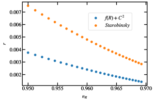
Figure 1: The graph represents the spectral tilt of the scalar perturbations $n_{\mathcal{R}}$ and the tensor to scalar ratio $r=A_{T}/A_{\mathcal{R}}$ from $N=40$ to $N=70$ number of e-folds. One can see the QG suppression of the tensor perturbations.

Power spectrum of PGWs: The next generation of ground-based GW detectors [25, 29, 30] and LISA [27] are expected to deliver data that will help to answer some of the deep questions in fundamental physics, astrophysics, and cosmology [101]. Modified theories of gravity have shown an impact on the PGWs power spectrum [102, 103]. Here, we show further that the quantum gravitational signatures in PGWs can potentially be observed in the next-generation gravitational wave detectors. Rewriting Eq. (15) as two second-order differential equations, in the Fourier domain, we have [96, 97]:

$$\frac{d^{2}\mu^{(1)}_{k}}{dz^{2}}+\left(1-\frac{2}{z^{2}}\right)\,\mu^{(1)}_{k}=0\,,$$ (22)

$$\frac{d^{2}\mu^{(2)}_{k}}{dz^{2}}+\left(1+\frac{1}{\gamma\,H^{2}\,z^{2}}\right)\,\mu^{(2)}_{k}=0\,,$$

where $\mu^{(1)}$ ($\mu^{(2)}$) corresponds to the standard gravitational wave (massive spin-2 mode from the modified theory), and $z\equiv-k\eta$. For pure de Sitter, the power spectrum can be evaluated exactly [104, 105] and is given by:

$$\mathcal{P}_{\rm PGW}(k) =\mathcal{P}_{0}(\gamma_{0},H)\left[1+\left[\frac{k}{k_{*}}\right]^{2}\right.$$ (23)

$$\left.-\frac{\pi}{2}\,\left[\frac{k}{k_{*}}\right]^{3}\!\!|\mathrm{e}^{\mathrm{i}\pi\,\nu/2}\,H^{(1)}_{\nu}\left[\frac{k}{k_{*}}\right]|^{2}\right],$$ (24)

where $\mathcal{P}_{0}(\gamma_{0},H)=(2\kappa\,H^{2}/\pi^{2})(1+2\gamma\,H^{2})$, $k_{*}=aH$ is the wavenumber at horizon crossing, $H^{(1)}_{\nu}$ is the Henkel function of the first kind, $H$ is the Hubble scale during inflation and $\nu=\frac{1}{4}\sqrt{1-\frac{4}{\gamma H^{2}}}$. The power spectrum given in Eq. (24) is valid for $\gamma_{0}>0$. For $\gamma_{0}=0$, the unmodified power spectrum for the PGWs is:

$$\mathcal{P}_{\rm PGW}(k)=\mathcal{P}_{0}(\gamma_{0},H)\left(\frac{k}{k_{*}}\right)^{n_{T}}\,.$$ (25)

Evaluating the power spectrum at the horizon crossing (i.e., $\eta\rightarrow 0$), for three values of $\gamma_{0}$ — $\{\gamma_{0}=0,\gamma_{0}^{N=40}$ and $\gamma_{0}^{N=60}\}$ (21) — we obtain the following values for the normalization constant $\mathcal{P}_{0}(\gamma_{0},H)$:

$$\mathcal{P}_{0}(\gamma_{0}=0,H=10^{15}{\rm GeV}) =1.329\times 10^{-25}$$ (26a)

$$\mathcal{P}_{0}(\gamma_{0,N=40},H=10^{15}{\rm GeV}) =4.841\times 10^{-29}$$ (26b)

$$\mathcal{P}_{0}(\gamma_{0,N=60},H=10^{15}{\rm GeV}) =2.152\times 10^{-29}\,,$$ (26c)

Fig. 2 contains the plot of the power spectrum of PGWs (for three different values of $\gamma_{0}$) as a function of frequency. From the figure, we infer that the power spectrum is almost constant for a large range of frequencies and is consistent with standard inflationary scenario [106]. Also, the degenerate Stelle gravity model suppresses the amplitude of PGWs. This implies that the longer the inflation, the larger the suppression of the amplitude of the PGWs. This is because the massive spin-2 modes carry less energy than the scalar modes [85]. Further, to quantify the detectability of PGWs in the upcoming GW detectors, we evaluate the energy density of PGWs [107]:

$$\Omega_{\text{GW}}(k)=\mathcal{P}_{\rm PGW}(k)\,(k^{2}/{(12H_{0}^{2})})\,.$$ (27)

where we have set the scale factor at the present time to unity,and $H_{0}=100\,h\,\text{km}\,\text{s}^{-1}\,\text{Mpc}^{-1}$. Figure 2 contains the plot of differential energy density is ${d(\Omega_{\text{GW}}(k))}/d\ln(k)$ as a function of $f$. From the figure, we infer that the differential energy density is 8-orders of magnitude larger in $kHz$ compared to $1~{}Hz$ range for all three values of $\gamma_{0}$. To confirm this, we now compare the projected characteristic strain for PGWs and the characteristic strain of the detectors. The characteristic strain of the PGWs is given by [108]:

$$h_{PGW}=\int\mathcal{P}_{\rm PGW}(f)\,df\,.$$ (28)

where $\mathcal{P}_{\rm PGW}(f)$ is given by Eq. (24). Since $\mathcal{P}_{\rm PGW}(f)$ is approximately constant with frequency (cf. Figure 2), we approximate $\mathcal{P}_{\rm PGW}(f)\approx\mathcal{P}_{0}(H,\gamma_{0})$. Thus, we get:

$$h_{PGW}\approx f\,\mathcal{P}_{0}(H,\gamma_{0})\,.$$ (29)

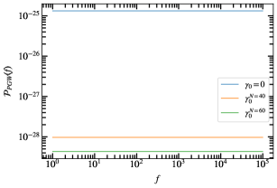
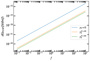
Figure 2: The top graph shows a logarithmic plot of the power spectrum $\mathcal{P}_{\rm PGW}(f)$ as a function of the frequency $f$ and the GUP parameter $\gamma_{0}$. The bottom graph shows the differential energy density of PGWs as a function of frequency.

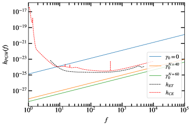
Figure 3: Logarithmic graph of the characteristic strain of the gravitational waves produced during inflation $h_{GW}$ as a function of frequency $f$ and the GUP parameter $\gamma_{0}$, compared to the characteristic strain of ET $h_{ET}$ [25] and CE $h_{CE}$ [29, 30].

Figure 3 contains the characteristic strain of PGWs for three different values of $\gamma_{0}$ (corresponding to different e-foldings of inflation) along with the design sensitivity of ET  [25] and CE  [29, 30]. From the figure, we infer the following: First, the characteristic strain of PGWs for the standard inflation (blue curve) is well within the observational capability of both ET and CE. Second, for degenerate Stelle gravity, as the number of e-foldings increases, the suppression of the amplitude of the PGWs is larger (orange and green curves). Hence, it is not possible to confirm their detection with confidence. However, the non-detectability of the PGWs will directly constrain the value of $\gamma_{0}$. Thus, ET [25] and CE [29, 30] can put a severe constraints on the value of the GUP parameter. Third, our analysis shows that LISA will not be able to detect PGWs as the characteristic strain is much larger than PGWs in low-frequency ($\sim 1~{}{\rm Hz}$). Lastly and most importantly, our analysis explicitly shows that we can strongly constrain the number of e-foldings of inflation from ET and CE.

Conclusions In conclusion, we demonstrated that our model is described by a linear combination of $f(R)$ gravity, particularly the Starobinsky model and Weyl-squared gravity. This allowed us to use the fakeon procedure [95] to obtain the scalar spectral tilt $n_{\mathcal{R}}$ and the tensor-scalar ratio $r$. Although our model and Starobinsky model are identical in the background FRW universe, they lead to different observable consequences in the linear order in perturbations. More specifically, we showed that the introduction of $R_{\mu\nu}R^{\mu\nu}$ decreases the ratio between the scalar contribution and the tensor modes. This is consistent with the recent analysis [85]. Using PLANCK observations, we determined the bounds on the GUP parameter $\gamma_{0}$. These bounds are consistent with bounds derived from other analysis [81, 80, 89, 90, 87, 88].

Later, using the constraint on $\gamma_{0}$ from the CMB observations, we explicitly showed that PWGs carry quantum gravitational signatures in their power spectrum and energy density. Furthermore, from Figure 3 one can conclude that these quantum gravitational effects will potentially be observable in the next-generation ground-based gravitational wave detectors such as ET and CE. Additionally, depending on the energy density of detected PGWs, one can strongly constrain the number of e-foldings of inflation using these detectors.

After the historical detection of GWs in the frequency range $100-10^{4}~{}{\rm Hz}$, there is a surge in activity for the possibility of detection of GWs in the MHz-GHz frequency range [109]. As mentioned earlier, for a large frequency range, $\mathcal{P}_{\rm PGW}$ is approximately constant. This means that high-frequency GW detectors with sensitivity around $10^{-20}$ can potentially detect PGWs. Such detectors will reveal a disparate view of the early universe compared to their electromagnetic counterparts.

Acknowledgments: The authors thank Avijit Chowdhury, Ashu Kushwaha, Abhishek Naskar and Vijay Nenmeli for their comments on the earlier draft. This work was supported by the Natural Sciences and Engineering Research Council of Canada. SS is supported by SERB-MATRICS grant.

Appendix

From the Relativistic GUP (RGUP) relation (1), it is clear that the position and momentum operators are no longer canonically conjugate. The introduction of a ”canonical” 4-momentum $p_{0}^{\mu}$ satisfying $[x^{\mu},p_{0}^{\nu}]=i\eta^{\mu\nu}$ simplifies calculations considerably. The ”physical” 4-momentum $p^{\mu}$ can be expressed in terms of $p_{0}^{\mu}$ as:

$$p^{\mu}=p_{0}^{\mu}(1-\gamma p_{0\nu}p_{0}^{\nu}).$$ (30)

In Ref. [81], we used the field theoretic approach to obtain a one-to-one correspondence between RGUP modified Spin-2 field theory and modified gravity:

1. The Lagrangian for a free spin-2 field must be bilinear in the field and its derivatives, $h_{\mu\nu}$. Relevant bilinears are readily enumerated.

2. Due to the long range of gravitational force, the mediating gauge bosons must be massless. Thus, we can assume that the Lagrangian consists solely of field derivatives and has no mass term.

3. We can create a minimal list by identifying pairs of bilinears that differ by surface terms. Thus, we can fix the action up to coefficients that are undetermined:

   $$\mathcal{L}=ah_{\mu\nu,\sigma}h^{\mu\nu,\sigma}+bh_{\mu\nu}\,^{,\nu}h^{\mu\sigma}\,_{,\sigma}+ch_{\mu\nu}\,^{,\nu}h^{\sigma}\,_{\sigma,\mu}+dh_{\mu}\,^{\mu}\,{}_{,\sigma}h^{\nu}\,_{\nu}\,{}^{,\sigma}$$

4. An interaction term of the form $\lambda h_{\mu\nu}T^{\mu\nu}$ takes into account the matter-gravity interactions. By adding this term to the preceding action and enforcing energy-momentum conservation (i.e. $\partial_{\mu}T^{\mu\nu}=0$), we obtain the following result:

   $$(2a+b)\Box h_{\mu\nu}\,^{\nu}+(b+c)h_{\nu\sigma}^{,\nu\sigma}\,{}_{,\mu}+(c+2d)\Box h_{\nu}\,^{\nu}\,{}_{,\mu}=0$$ (31)

   We can use the above expression to fix the coefficients.

The Lagrangian corresponding to the above EOM is

$$\mathcal{L}_{free}=\frac{1}{2}h_{\mu\nu,\sigma}h^{\mu\nu,\sigma}-h_{\mu\nu}\,^{,\nu}h^{\mu\sigma}\,_{,\sigma}+h_{\mu\nu}\,^{,\nu}h^{\sigma}\,_{\sigma,\mu}-\frac{1}{2}h_{\mu}\,^{\mu}\,{}_{,\sigma}h^{\nu}\,_{\nu}\,{}^{,\sigma}$$ (32)

The RGUP modified EOM are obtained from the position space representation of (30) (i.e. $\partial_{\mu}\rightarrow\partial_{\mu}(1-\gamma\Box)$). We have

$$G^{L}_{\mu\nu}+\gamma\mathcal{G}_{\mu\nu}=0,$$ (33)

where

$$\!\!\!\!\!\!\!\!\!\!\!\!\!\!\!\!\!\!\!\!\!\!\!\!\!G^{L}_{\mu\nu}=\Box h_{\mu\nu}-h_{\mu\sigma,\nu}^{\sigma}-h_{\nu\sigma,\mu}^{\sigma}+h_{\sigma,\mu\nu}\,^{\sigma}+\eta_{\mu\nu}h_{\sigma\rho}^{,\sigma\rho}-\eta_{\mu\nu}\Box h_{\sigma}^{\sigma},$$ (35)

$$\!\!\!\!\!\!\!\!\!\!\!\!\!\!\!\!\!\!\!\!\!\!\!\!\!\mathcal{G}_{\mu\nu}=\Box^{2}h_{\mu\nu}-\Box h_{\mu\sigma,\nu}^{,\sigma}-h_{\nu\sigma\mu}^{,\sigma}.+\Box h_{\sigma,\mu\nu}^{,\sigma}+\eta_{\mu\nu}h_{\sigma\rho}^{,\sigma\rho}-\eta_{\mu\nu}\Box^{2}h_{\sigma}^{\sigma}.~{}~{}$$

The above linearized equation of motion is identical to the equations of motion obtained by linearlized Stelle action [83, 81]:

$$S=\int\,d^{4}x\,\sqrt{-g}\left[\frac{1}{2\kappa^{2}}R-\alpha\,R^{\mu\nu}R_{\mu\nu}+\beta\,R^{2}\right]\,.$$

We showed that the linearized Stelle gravity equations of motion match (33) perfectly when $\alpha=2\beta=\gamma/\kappa^{2}$. In other words, we showed that $\alpha=2\beta$ Stelle gravity is the minimally modified, metric-only theory of gravity which models the effects of maximal momentum. Hence, the model we have used is a one-parameter model, and this equality is then translated into the $f(R)+C^{2}$ model that we used for the modeling of our inflation parameters.

References

- Smoot et al. [1992] G. F. Smoot, et al. (COBE), Structure in the COBE differential microwave radiometer first year maps, Astrophys. J. Lett. 396 (1992) L1–L5. doi:10.1086/186504.
- de Bernardis et al. [2000] P. de Bernardis, et al. (Boomerang), A Flat universe from high resolution maps of the cosmic microwave background radiation, Nature 404 (2000) 955–959. doi:10.1038/35010035. arXiv:astro-ph/0004404.
- Spergel et al. [2003] D. N. Spergel, et al. (WMAP), First year Wilkinson Microwave Anisotropy Probe (WMAP) observations: Determination of cosmological parameters, Astrophys. J. Suppl. 148 (2003) 175–194. doi:10.1086/377226. arXiv:astro-ph/0302209.
- Ogburn et al. [2010] R. W. Ogburn, et al., The BICEP2 CMB polarization experiment, in: W. S. Holland, J. Zmuidzinas (Eds.), Millimeter, Submillimeter, and Far-Infrared Detectors and Instrumentation for Astronomy V, volume 7741, SPIE, 2010, pp. 415 – 425. URL: https://doi.org/10.1117/12.857864. doi:10.1117/12.857864.
- Aghanim et al. [2020] N. Aghanim, et al. (Planck), Planck 2018 results. I. Overview and the cosmological legacy of Planck, Astron. Astrophys. 641 (2020) A1. doi:10.1051/0004-6361/201833880. arXiv:1807.06205.
- Akrami et al. [2020] Y. Akrami, et al. (Planck), Planck 2018 results. X. Constraints on inflation, Astron. Astrophys. 641 (2020) A10. doi:10.1051/0004-6361/201833887. arXiv:1807.06211.
- Ade et al. [2021] P. A. R. Ade, et al. (BICEP/Keck Collaboration), Improved constraints on primordial gravitational waves using planck, wmap, and bicep/keck observations through the 2018 observing season, Phys. Rev. Lett. 127 (2021) 151301. URL: https://link.aps.org/doi/10.1103/PhysRevLett.127.151301. doi:10.1103/PhysRevLett.127.151301.
- Starobinsky [1980] A. A. Starobinsky, A new type of isotropic cosmological models without singularity, Phys. Lett. B91 (1980) 99–102. doi:10.1016/0370-2693(80)90670-X.
- Kodama and Sasaki [1984] H. Kodama, M. Sasaki, Cosmological Perturbation Theory, Prog. Theor. Phys. Suppl. 78 (1984) 1–166. doi:10.1143/PTPS.78.1.
- Mukhanov et al. [1992] V. F. Mukhanov, H. A. Feldman, R. H. Brandenberger, Theory of cosmological perturbations. Part 1. Classical perturbations. Part 2. Quantum theory of perturbations. Part 3. Extensions, Phys. Rept. 215 (1992) 203–333. doi:10.1016/0370-1573(92)90044-Z.
- Lidsey et al. [1997] J. E. Lidsey, A. R. Liddle, E. W. Kolb, E. J. Copeland, T. Barreiro, M. Abney, Reconstructing the inflation potential : An overview, Rev. Mod. Phys. 69 (1997) 373–410. doi:10.1103/RevModPhys.69.373. arXiv:astro-ph/9508078.
- Lyth and Riotto [1999] D. H. Lyth, A. Riotto, Particle physics models of inflation and the cosmological density perturbation, Phys. Rept. 314 (1999) 1–146. doi:10.1016/S0370-1573(98)00128-8. arXiv:hep-ph/9807278.
- Bassett et al. [2006] B. A. Bassett, S. Tsujikawa, D. Wands, Inflation dynamics and reheating, Rev. Mod. Phys. 78 (2006) 537–589. doi:10.1103/RevModPhys.78.537. arXiv:astro-ph/0507632.
- Grishchuk and Sidorov [1990] L. P. Grishchuk, Y. V. Sidorov, Squeezed quantum states of relic gravitons and primordial density fluctuations, Phys. Rev. D 42 (1990) 3413–3421. doi:10.1103/PhysRevD.42.3413.
- Sathyaprakash and Schutz [2009] B. S. Sathyaprakash, B. F. Schutz, Physics, Astrophysics and Cosmology with Gravitational Waves, Living Rev. Rel. 12 (2009) 2. doi:10.12942/lrr-2009-2. arXiv:0903.0338.
- Guzzetti et al. [2016] M. C. Guzzetti, N. Bartolo, M. Liguori, S. Matarrese, Gravitational waves from inflation, Riv. Nuovo Cim. 39 (2016) 399–495. doi:10.1393/ncr/i2016-10127-1. arXiv:1605.01615.
- Baumann et al. [2009] D. Baumann, et al. (CMBPol Study Team), CMBPol Mission Concept Study: Probing Inflation with CMB Polarization, AIP Conf. Proc. 1141 (2009) 10–120. doi:10.1063/1.3160885. arXiv:0811.3919.
- Crill et al. [2008] B. P. Crill, et al., SPIDER: A Balloon-borne Large-scale CMB Polarimeter, Proc. SPIE Int. Soc. Opt. Eng. 7010 (2008) 70102P. doi:10.1117/12.787446. arXiv:0807.1548.
- Eimer et al. [2012] J. R. Eimer, et al., The cosmology large angular scale surveyor (CLASS): 40 GHz optical design, in: W. S. Holland, J. Zmuidzinas (Eds.), Millimeter, Submillimeter, and Far-Infrared Detectors and Instrumentation for Astronomy VI, volume 8452 of Society of Photo-Optical Instrumentation Engineers (SPIE) Conference Series, 2012, p. 845220. doi:10.1117/12.925464. arXiv:1211.0041.
- Ade et al. [2015] P. A. R. Ade, et al. (BICEP2, Planck), Joint Analysis of BICEP2/ and Data, Phys. Rev. Lett. 114 (2015) 101301. doi:10.1103/PhysRevLett.114.101301. arXiv:1502.00612.
- Ade et al. [2014] P. A. R. Ade, et al. (POLARBEAR), A Measurement of the Cosmic Microwave Background B-Mode Polarization Power Spectrum at Sub-Degree Scales with POLARBEAR, Astrophys. J. 794 (2014) 171. doi:10.1088/0004-637X/794/2/171. arXiv:1403.2369, [Erratum: Astrophys.J. 848, 73 (2017)].
- Gandilo et al. [2016] N. N. Gandilo, et al., The Primordial Inflation Polarization Explorer (PIPER), in: W. S. Holland, J. Zmuidzinas (Eds.), Millimeter, Submillimeter, and Far-Infrared Detectors and Instrumentation for Astronomy VIII, volume 9914 of Society of Photo-Optical Instrumentation Engineers (SPIE) Conference Series, 2016, p. 99141J. doi:10.1117/12.2231109. arXiv:1607.06172.
- Paoletti et al. [2022] D. Paoletti, F. Finelli, J. Valiviita, M. Hazumi, Planck and BICEP/Keck Array 2018 constraints on primordial gravitational waves and perspectives for future B-mode polarization measurements (2022). arXiv:2208.10482.
- Crowder and Cornish [2005] J. Crowder, N. J. Cornish, Beyond LISA: Exploring future gravitational wave missions, Phys. Rev. D 72 (2005) 083005. doi:10.1103/PhysRevD.72.083005. arXiv:gr-qc/0506015.
- Hild et al. [2011] S. Hild, et al., Sensitivity Studies for Third-Generation Gravitational Wave Observatories, Class. Quant. Grav. 28 (2011) 094013. doi:10.1088/0264-9381/28/9/094013. arXiv:1012.0908.
- Sato et al. [2017] S. Sato, et al., The status of DECIGO, J. Phys. Conf. Ser. 840 (2017) 012010. doi:10.1088/1742-6596/840/1/012010.
- Amaro-Seoane et al. [2017] P. Amaro-Seoane, et al., Laser Interferometer Space Antenna, arXiv e-prints (2017) arXiv:1702.00786. arXiv:1702.00786.
- Maggiore et al. [2020] M. Maggiore, et al., Science Case for the Einstein Telescope, JCAP 03 (2020) 050. doi:10.1088/1475-7516/2020/03/050. arXiv:1912.02622.
- Evans et al. [2021] M. Evans, et al., A Horizon Study for Cosmic Explorer: Science, Observatories, and Community (2021). arXiv:2109.09882.
- Srivastava et al. [2022] V. Srivastava, D. Davis, K. Kuns, P. Landry, S. Ballmer, M. Evans, E. D. Hall, J. Read, B. S. Sathyaprakash, Science-driven Tunable Design of Cosmic Explorer Detectors, Astrophys. J. 931 (2022) 22. doi:10.3847/1538-4357/ac5f04. arXiv:2201.10668.
- Garay [1995] L. J. Garay, Quantum gravity and minimum length, Int. J. Mod. Phys. A 10 (1995) 145–166. doi:10.1142/S0217751X95000085. arXiv:gr-qc/9403008.
- Hossenfelder [2013] S. Hossenfelder, Minimal Length Scale Scenarios for Quantum Gravity, Living Rev. Rel. 16 (2013) 2. doi:10.12942/lrr-2013-2. arXiv:1203.6191.
- Addazi et al. [2022] A. Addazi, et al., Quantum gravity phenomenology at the dawn of the multi-messenger era—A review, Prog. Part. Nucl. Phys. 125 (2022) 103948. doi:10.1016/j.ppnp.2022.103948. arXiv:2111.05659.
- Adler and Santiago [1999] R. J. Adler, D. I. Santiago, On gravity and the uncertainty principle, Mod. Phys. Lett. A 14 (1999) 1371. URL: http://dx.doi.org/10.1142/S0217732399001462. doi:10.1142/S0217732399001462.
- Adler et al. [2001] R. J. Adler, P. Chen, D. I. Santiago, The generalized uncertainty principle and black hole remnants, Gen. Relat. Grav. 33 (2001) 2101–2108. URL: http://dx.doi.org/10.1023/A:1015281430411. doi:10.1023/a:1015281430411.
- Ali and Majumder [2014] A. F. Ali, B. Majumder, Towards a cosmology with minimal length and maximal energy, Class. Quant. Grav. 31 (2014) 215007. URL: http://dx.doi.org/10.1088/0264-9381/31/21/215007. doi:10.1088/0264-9381/31/21/215007.
- Ali et al. [2015] A. F. Ali, M. Faizal, M. M. Khalil, Short distance physics of the inflationary de sitter universe, JCAP 2015 (2015) 025–025. URL: http://dx.doi.org/10.1088/1475-7516/2015/09/025. doi:10.1088/1475-7516/2015/09/025.
- Alonso-Serrano et al. [2018] A. Alonso-Serrano, M. P. Dabrowski, H. Gohar, Generalized uncertainty principle impact onto the black holes information flux and the sparsity of hawking radiation, Phys. Rev. D 97 (2018). URL: http://dx.doi.org/10.1103/PhysRevD.97.044029. doi:10.1103/physrevd.97.044029.
- Amati et al. [1989] D. Amati, M. Ciafaloni, G. Veneziano, Can spacetime be probed below the string size?, Phys. Lett. B 216 (1989) 41–47. URL: https://www.sciencedirect.com/science/article/pii/037026938991366X. doi:10.1016/0370-2693(89)91366-X.
- Amelino-Camelia [2013] G. Amelino-Camelia, Quantum-Spacetime phenomenology, Living Rev. Relativ. 16 (2013) 5. URL: http://dx.doi.org/10.12942/lrr-2013-5. doi:10.12942/lrr-2013-5.
- Bargueño and Vagenas [2015] P. Bargueño, E. C. Vagenas, Semiclassical corrections to black hole entropy and the generalized uncertainty principle, Phys. Letts. B 742 (2015) 15–18. URL: http://dx.doi.org/10.1016/j.physletb.2015.01.016. doi:10.1016/j.physletb.2015.01.016.
- Bambi and Urban [2007] C. Bambi, F. R. Urban, Natural extension of the generalised uncertainty principle, Class. Quant. Grav. 25 (2007) 095006. URL: http://dx.doi.org/10.1088/0264-9381/25/9/095006. doi:10.1088/0264-9381/25/9/095006.
- Bawaj et al. [2015] M. Bawaj, C. Biancofiore, M. Bonaldi, F. Bonfigli, A. Borrielli, G. Di Giuseppe, L. Marconi, F. Marino, R. Natali, A. Pontin, et al., Probing deformed commutators with macroscopic harmonic oscillators, Nature Communications 6 (2015). URL: http://dx.doi.org/10.1038/ncomms8503.
- Bojowald and Kempf [2011] M. Bojowald, A. Kempf, Generalized uncertainty principles and localization of a particle in discrete space, Phys. Rev. D 86 (2011) 085017. URL: http://dx.doi.org/10.1103/PhysRevD.86.085017. doi:10.1103/PhysRevD.86.085017.
- Bolen and Cavagliá [2005] B. Bolen, M. Cavagliá, (anti-)de sitter black hole thermodynamics and the generalized uncertainty principle, Gen. Relat. Grav. 37 (2005) 1255–1262. URL: https://doi.org/10.1007/s10714-005-0108-x. doi:10.1007/s10714-005-0108-x.
- Bosso and Das [2017] P. Bosso, S. Das, Generalized uncertainty principle and angular momentum, Annals of Physics 383 (2017) 416–438.
- Bosso et al. [2018] P. Bosso, S. Das, R. B. Mann, Potential tests of the Generalized Uncertainty Principle in the advanced LIGO experiment, Phys. Lett. B 785 (2018) 498–505. doi:10.1016/j.physletb.2018.08.061. arXiv:1804.03620.
- Bosso [2018] P. Bosso, Rigorous Hamiltonian and Lagrangian analysis of classical and quantum theories with minimal length, Phys. Rev. D 97 (2018) 126010. doi:10.1103/PhysRevD.97.126010. arXiv:1804.08202.
- Bosso and Obregón [2020] P. Bosso, O. Obregón, Minimal length effects on quantum cosmology and quantum black hole models, Class. Quant. Grav. 37 (2020) 045003. doi:10.1088/1361-6382/ab6038. arXiv:1904.06343.
- Burger et al. [2018] D. J. Burger, N. Moynihan, S. Das, S. Shajidul Haque, B. Underwood, Towards the Raychaudhuri Equation Beyond General Relativity, Phys. Rev. D 98 (2018) 024006. doi:10.1103/PhysRevD.98.024006. arXiv:1802.09499.
- Bushev et al. [2019] P. Bushev, J. Bourhill, M. Goryachev, N. Kukharchyk, E. Ivanov, S. Galliou, M. Tobar, S. Danilishin, Testing the generalized uncertainty principle with macroscopic mechanical oscillators and pendulums, Phys. Rev. D 100 (2019) 066020.
- Casadio and Scardigli [2020] R. Casadio, F. Scardigli, Generalized uncertainty principle, classical mechanics, and general relativity, Phys. Letts. B 807 (2020) 135558. URL: http://dx.doi.org/10.1016/j.physletb.2020.135558. doi:10.1016/j.physletb.2020.135558.
- Chang et al. [2011] L. N. Chang, Z. Lewis, D. Minic, T. Takeuchi, On the Minimal Length Uncertainty Relation and the Foundations of String Theory, Adv. High Energy Phys. 2011 (2011) 493514. doi:10.1155/2011/493514. arXiv:1106.0068.
- Cortes and Gamboa [2005] J. L. Cortes, J. Gamboa, Quantum uncertainty in doubly special relativity, Phys. Rev. D 71 (2005) 065015. doi:10.1103/PhysRevD.71.065015. arXiv:hep-th/0405285.
- Costa Filho et al. [2016] R. N. Costa Filho, J. P. M. Braga, J. H. S. Lira, J. S. Andrade, Extended uncertainty from first principles, Phys. Lett. B 755 (2016) 367–370. URL: https://www.sciencedirect.com/science/article/pii/S0370269316001313. doi:10.1016/j.physletb.2016.02.035.
- Dabrowski and Wagner [2020] M. P. Dabrowski, F. Wagner, Asymptotic generalized extended uncertainty principle, Eur. Phys. J. C 80 (2020) 676. URL: http://dx.doi.org/10.1140/epjc/s10052-020-8250-x. doi:10.1140/epjc/s10052-020-8250-x.
- Das and Vagenas [2008] S. Das, E. C. Vagenas, Universality of Quantum Gravity Corrections, Phys. Rev. Lett. 101 (2008) 221301. doi:10.1103/PhysRevLett.101.221301.
- Das et al. [2010] S. Das, E. C. Vagenas, A. F. Ali, Discreteness of Space from GUP II: Relativistic Wave Equations, Phys. Lett. B 690 (2010) 407–412. doi:10.1016/j.physletb.2010.05.052, [Erratum: Phys.Lett.B 692, 342–342 (2010)].
- Das et al. [2019] S. Das, S. S. Haque, B. Underwood, Constraints and horizons for de sitter with extra dimensions, Phys. Rev. D 100 (2019). URL: http://dx.doi.org/10.1103/PhysRevD.100.046013.
- Das et al. [2020] A. Das, S. Das, E. C. Vagenas, Discreteness of space from gup in strong gravitational fields, Phys. Letts. B 809 (2020) 135772. URL: http://dx.doi.org/10.1016/j.physletb.2020.135772. doi:10.1016/j.physletb.2020.135772.
- Garcia-Chung et al. [2021] A. Garcia-Chung, J. B. Mertens, S. Rastgoo, Y. Tavakoli, P. Vargas Moniz, Propagation of quantum gravity-modified gravitational waves on a classical FLRW spacetime, Phys. Rev. D 103 (2021) 084053. doi:10.1103/PhysRevD.103.084053. arXiv:2012.09366.
- Giddings [2020] S. B. Giddings, Black holes and other clues to the quantum structure of gravity, Galaxies 9 (2020) 16. URL: http://dx.doi.org/10.3390/galaxies9010016. doi:10.3390/galaxies9010016.
- Hamil et al. [2019] B. Hamil, M. Merad, T. Birkandan, Applications of the extended uncertainty principle in AdS and ds spaces, Eur. Phys. J. Plus 134 (2019) 278. URL: https://doi.org/10.1140/epjp/i2019-12633-y. doi:10.1140/epjp/i2019-12633-y.
- Hossenfelder [2006] S. Hossenfelder, Interpretation of quantum field theories with a minimal length scale, Phys. Rev. D 73 (2006) 105013. doi:10.1103/PhysRevD.73.105013.
- Kempf et al. [1995] A. Kempf, G. Mangano, R. B. Mann, Hilbert space representation of the minimal length uncertainty relation, Phys. Rev. D Part. Fields 52 (1995) 1108–1118. URL: http://dx.doi.org/10.1103/physrevd.52.1108. doi:10.1103/physrevd.52.1108.
- Kober [2010] M. Kober, Gauge Theories under Incorporation of a Generalized Uncertainty Principle, Phys. Rev. D 82 (2010) 085017. doi:10.1103/PhysRevD.82.085017.
- Konishi et al. [1990] K. Konishi, G. Paffuti, P. Provero, Minimum physical length and the generalized uncertainty principle in string theory, Phys. Letts. B 234 (1990) 276 – 284. URL: http://www.sciencedirect.com/science/article/pii/0370269390919274. doi:https://doi.org/10.1016/0370-2693(90)91927-4.
- Maggiore [1993] M. Maggiore, A generalized uncertainty principle in quantum gravity, Phys. Letts. B 304 (1993) 65 – 69. URL: http://www.sciencedirect.com/science/article/pii/0370269393914018. doi:https://doi.org/10.1016/0370-2693(93)91401-8.
- Marin et al. [2013] F. Marin, et al., Gravitational bar detectors set limits to Planck-scale physics on macroscopic variables, Nature Phys. 9 (2013) 71–73. doi:10.1038/nphys2503.
- Moradpour et al. [2021] H. Moradpour, S. Aghababaei, A. H. Ziaie, A note on effects of generalized and extended uncertainty principles on jüttner gas, Symmetry 13 (2021) 213. URL: https://www.mdpi.com/2073-8994/13/2/213. doi:10.3390/sym13020213.
- Mureika [2019] J. R. Mureika, Extended uncertainty principle black holes, Phys. Lett. B 789 (2019) 88–92. URL: https://www.sciencedirect.com/science/article/pii/S037026931830933X. doi:10.1016/j.physletb.2018.12.009.
- Myung et al. [2007] Y. S. Myung, Y.-W. Kim, Y.-J. Park, Black hole thermodynamics with generalized uncertainty principle, Phys. Letts. B 645 (2007) 393–397. URL: http://dx.doi.org/10.1016/j.physletb.2006.12.062. doi:10.1016/j.physletb.2006.12.062.
- Park [2008] M.-I. Park, The generalized uncertainty principle in (A)dS space and the modification of hawking temperature from the minimal length, Phys. Lett. B 659 (2008) 698–702. URL: https://www.sciencedirect.com/science/article/pii/S0370269307014980. doi:10.1016/j.physletb.2007.11.090.
- Snyder [1947] H. S. Snyder, Quantized space-time, Phys. Rev. 71 (1947) 38–41. URL: https://link.aps.org/doi/10.1103/PhysRev.71.38. doi:10.1103/PhysRev.71.38.
- Sprenger et al. [2011] M. Sprenger, P. Nicolini, M. Bleicher, Neutrino oscillations as a novel probe for a minimal length, Class. Quant. Grav. 28 (2011) 235019. URL: http://dx.doi.org/10.1088/0264-9381/28/23/235019. doi:10.1088/0264-9381/28/23/235019.
- Jaffino Stargen et al. [2019] D. Jaffino Stargen, S. Shankaranarayanan, S. Das, Polymer quantization and advanced gravitational wave detector, Phys. Rev. D 100 (2019) 086007. doi:10.1103/PhysRevD.100.086007. arXiv:1907.05863.
- Wang et al. [2016] B. Wang, C. Long, Z. Long, T. Xu, Solutions of the schrödinger equation under topological defects space-times and generalized uncertainty principle, The European Physical Journal Plus 131 (2016) 378.
- Bosso et al. [2020a] P. Bosso, S. Das, V. Todorinov, Quantum field theory with the generalized uncertainty principle i: Scalar electrodynamics, Ann. Phys. 422 (2020a) 168319. URL: http://dx.doi.org/10.1016/j.aop.2020.168319. doi:10.1016/j.aop.2020.168319.
- Bosso et al. [2020b] P. Bosso, S. Das, V. Todorinov, Quantum field theory with the generalized uncertainty principle II: Quantum electrodynamics, Ann. Phys. 424 (2020b) 168350. URL: http://dx.doi.org/10.1016/j.aop.2020.168350. doi:10.1016/j.aop.2020.168350.
- Todorinov et al. [2018] V. Todorinov, P. Bosso, S. Das, Relativistic generalized uncertainty principle, Ann. Phys. 405 (2018) 92–100. URL: http://dx.doi.org/10.1016/j.aop.2019.03.014. doi:10.1016/j.aop.2019.03.014.
- Nenmeli et al. [2021] V. Nenmeli, S. Shankaranarayanan, V. Todorinov, S. Das, Maximal momentum GUP leads to quadratic gravity, Phys. Lett. B 821 (2021) 136621. doi:10.1016/j.physletb.2021.136621. arXiv:2106.04141.
- Stelle [1978] K. S. Stelle, Classical gravity with higher derivatives, Gen. Relat. Grav. 9 (1978) 353–371. URL: https://doi.org/10.1007/BF00760427. doi:10.1007/BF00760427.
- Stelle [1977] K. S. Stelle, Renormalization of higher-derivative quantum gravity, Phys. Rev. D 16 (1977) 953–969. URL: https://link.aps.org/doi/10.1103/PhysRevD.16.953. doi:10.1103/PhysRevD.16.953.
- Noakes [1983] D. R. Noakes, The initial value formulation of higher derivative gravity, J. Math. Phys. 24 (1983) 1846–1850. URL: https://doi.org/10.1063/1.525906. doi:10.1063/1.525906.
- Chowdhury et al. [2022] A. Chowdhury, S. Xavier, S. Shankaranarayanan, Massive tensor modes carry more energy than scalar modes in quadratic gravity (2022). arXiv:2206.06756.
- Ade et al. [2016] P. A. R. Ade, et al. (Planck), Planck 2015 results. XX. Constraints on inflation, Astron. Astrophys. 594 (2016) A20. doi:10.1051/0004-6361/201525898. arXiv:1502.02114.
- Das et al. [2022] S. Das, M. Fridman, G. Lambiase, E. C. Vagenas, Baryon asymmetry from the generalized uncertainty principle, Phys. Lett. B 824 (2022) 136841. doi:10.1016/j.physletb.2021.136841. arXiv:2107.02077.
- Das et al. [2021] A. Das, S. Das, N. R. Mansour, E. C. Vagenas, Bounds on GUP parameters from GW150914 and GW190521, Phys. Lett. B 819 (2021) 136429. doi:10.1016/j.physletb.2021.136429. arXiv:2101.03746.
- Bosso [2021] P. Bosso, On the quasi-position representation in theories with a minimal length, Class. Quant. Grav. 38 (2021) 075021. URL: https://doi.org/10.1088/1361-6382/abe758. doi:10.1088/1361-6382/abe758.
- Bosso et al. [2021] P. Bosso, O. Obregón, S. Rastgoo, W. Yupanqui, Deformed algebra and the effective dynamics of the interior of black holes, Class. Quant. Grav. 38 (2021) 145006. doi:10.1088/1361-6382/ac025f.
- Hawking and Ellis [1973] S. W. Hawking, G. F. R. Ellis, The Large Scale Structure of Space-Time, Cambridge Monographs on Mathematical Physics, Cambridge University Press, 1973. doi:10.1017/CBO9780511524646.
- Wald [1984] R. M. Wald, General Relativity, Chicago Univ. Pr., Chicago, USA, 1984. doi:10.7208/chicago/9780226870373.001.0001.
- Lovelock [1971] D. Lovelock, The Einstein tensor and its generalizations, J. Math. Phys. 12 (1971) 498–501. doi:10.1063/1.1665613.
- Sotiriou and Faraoni [2010] T. P. Sotiriou, V. Faraoni, f(R) Theories Of Gravity, Rev. Mod. Phys. 82 (2010) 451–497. doi:10.1103/RevModPhys.82.451. arXiv:0805.1726.
- Anselmi et al. [2020] D. Anselmi, E. Bianchi, M. Piva, Predictions of quantum gravity in inflationary cosmology: effects of the Weyl-squared term, JHEP 07 (2020) 211. doi:10.1007/JHEP07(2020)211. arXiv:2005.10293.
- Deruelle et al. [2011] N. Deruelle, M. Sasaki, Y. Sendouda, A. Youssef, Inflation with a Weyl term, or ghosts at work, JCAP 03 (2011) 040. doi:10.1088/1475-7516/2011/03/040. arXiv:1012.5202.
- Deruelle et al. [2012] N. Deruelle, M. Sasaki, Y. Sendouda, A. Youssef, Lorentz-violating vs ghost gravitons: the example of Weyl gravity, JHEP 09 (2012) 009. doi:10.1007/JHEP09(2012)009. arXiv:1202.3131.
- Anselmi [2017] D. Anselmi, On the quantum field theory of the gravitational interactions, JHEP 06 (2017) 086. doi:10.1007/JHEP06(2017)086. arXiv:1704.07728.
- Sasaki and Tagoshi [2003] M. Sasaki, H. Tagoshi, Analytic black hole perturbation approach to gravitational radiation, Living Rev. Relativ. 6 (2003) 6. URL: http://dx.doi.org/10.12942/lrr-2003-6. doi:10.12942/lrr-2003-6.
- Bonga and Gupt [2016] B. Bonga, B. Gupt, Phenomenological investigation of a quantum gravity extension of inflation with the Starobinsky potential, Phys. Rev. D 93 (2016) 063513. doi:10.1103/PhysRevD.93.063513. arXiv:1510.04896.
- Barack et al. [2019] L. Barack, et al., Black holes, gravitational waves and fundamental physics: a roadmap, Class. Quant. Grav. 36 (2019) 143001. doi:10.1088/1361-6382/ab0587. arXiv:1806.05195.
- Oikonomou [2022] V. K. Oikonomou, -Gravity Generated Post-inflationary Eras and their Effect on Primordial Gravitational Waves (2022). doi:10.1002/andp.202200134. arXiv:2205.15405.
- Odintsov et al. [2022] S. D. Odintsov, V. K. Oikonomou, R. Myrzakulov, Spectrum of Primordial Gravitational Waves in Modified Gravities: A Short Overview, Symmetry 14 (2022) 729. doi:10.3390/sym14040729. arXiv:2204.00876.
- Shankaranarayanan and Sriramkumar [2004] S. Shankaranarayanan, L. Sriramkumar, Trans-Planckian corrections to the primordial spectrum in the infrared and the ultraviolet, Phys. Rev. D 70 (2004) 123520. doi:10.1103/PhysRevD.70.123520. arXiv:hep-th/0403236.
- Sriramkumar and Shankaranarayanan [2006] L. Sriramkumar, S. Shankaranarayanan, Path integral duality and Planck scale corrections to the primordial spectrum in exponential inflation, JHEP 12 (2006) 050. doi:10.1088/1126-6708/2006/12/050. arXiv:hep-th/0608224.
- Turner [1997] M. S. Turner, Detectability of inflation produced gravitational waves, Phys. Rev. D 55 (1997) R435–R439. doi:10.1103/PhysRevD.55.R435. arXiv:astro-ph/9607066.
- Smith et al. [2006] T. L. Smith, M. Kamionkowski, A. Cooray, Direct detection of the inflationary gravitational wave background, Phys. Rev. D 73 (2006) 023504. doi:10.1103/PhysRevD.73.023504. arXiv:astro-ph/0506422.
- Moore et al. [2015] C. J. Moore, R. H. Cole, C. P. L. Berry, Gravitational-wave sensitivity curves, Class. Quant. Grav. 32 (2015) 015014. doi:10.1088/0264-9381/32/1/015014. arXiv:1408.0740.
- Aggarwal et al. [2021] N. Aggarwal, et al., Challenges and opportunities of gravitational-wave searches at MHz to GHz frequencies, Living Rev. Rel. 24 (2021) 4. doi:10.1007/s41114-021-00032-5.