Nematic Tomonaga-Luttinger Liquid Phase in an $S\!=\!1/2$ Ferromagnetic-Antiferromagnetic Bond-Alternating Chain

Abstract

We numerically investigate the ground-state phase diagram of the $S\!=\!1/2$ ferromagnetic-antiferromagnetic bond-alternating chain, in which the ferromagnetic interactions are stronger than the antiferromagnetic ones, and the anisotropies of the former and latter interactions are of the Ising-type and the $XY$-type, respectively. We use various numerical methods, such as the level spectroscopy and phenomenological renormalization-group analyses of the numerical data obtained by the exact diagonalization method, and so on. The resultant phase diagrams contain the ferromagnetic, $XY$1, singlet-dimer, and up-up-down-down phases as well as the nematic Tomonaga-Luttinger liquid (nTLL) phase which appears in a wide region of the interaction parameters. Perturbation calculations from the strong limit of the ferromagnetic interactions reproduce fairly well the numerical results of the phase boundary lines associated with the nTLL phase in the phase diagrams.

1 Introduction

Over the past several decades, a great deal of numerical, theoretical, and experimental work has been devoted to clarifying the quantum phase transition in one-dimensional $S\!=\!1/2$ systems. As is well known, due to the strong quantum fluctuation, a variety of exotic quantum phases appear in the ground-state phase diagrams of these systems. A typical example attracted recently much attention is the nematic Tomonaga-Luttinger liquid (nTLL) phase [1, 2, 3, 4, 5, 6, 7, 8, 9, 10, 11, 12], which is characterized not only by the formation of two-magnon bound pairs but also by the dominant nematic four-spin correlation function.

Recently, we[12] have numerically explored the ground-state phase diagram of an $S\!=\!1/2$ anisotropic two-leg ladder with different leg interactions in the absence of external magnetic field. This system has frustration when the signs of the two kinds of leg interactions are different from each other. Then, we have found that, when the ferromagnetic rung interactions with the Ising-type anisotropy is much stronger than the antiferromagnetic leg interactions with the $XY$-type anisotropy, the nTLL phase appears in the unfrustrated region as well as in the frustrated region. For this phase in the former region, the asymptotic form of the nematic correlation function shows the power-law decay with the uniform character; on the other hand, for this phase in the latter region, that shows the power-law decay with the staggered character. Thus, both nTLL phases are different phases. As far as we know, this is the first report of the realization of the nTLL phase in an $S\!=\!1/2$ unfrustrated one-dimensional spin system under no external magnetic field.

According to this result, it is reasonably expected that the nTLL state appears as the zero-field ground state in general $S\!=\!1/2$ unfrustrated one-dimensional systems in which pairs of $S\!=\!1/2$ spins coupled strongly with the Ising-type ferromagnetic interaction are connected by the weak antiferromagnetic interactions. As an example of such systems, we investigate in this paper an $S\!=\!1/2$ ferromagnetic-antiferromagnetic bond-alternating chain. We express the Hamiltonian describing this system as

$${\cal H}=-J_{{\rm F}}\sum_{j=1}^{N/2}\bigl{\{}\Gamma_{{\rm F}}\bigl{(}S_{2j-1}^{x}S_{2j}^{x}+S_{2j-1}^{y}S_{2j}^{y}\bigr{)}+S_{2j-1}^{z}S_{2j}^{z}\bigr{\}}+J_{\rm AF}\sum_{j=1}^{N/2}\bigl{\{}S_{2j}^{x}S_{2j+1}^{x}+S_{2j}^{y}S_{2j+1}^{y}+\Delta_{{\rm AF}}\,S_{2j}^{z}S_{2j+1}^{z}\bigr{\}}\,,$$ (1)

where $S_{j}^{\mu}$ ($\mu\!=\!x,y,z$) is the $\mu$-component of the $S\!=\!1/2$ operator $S$_j at the $j$th site; $J_{{\rm F}}$ and $J_{{\rm AF}}$ denote, respectively, the magnitudes of the ferromagnetic and antiferromagnetic interactions; $\Gamma_{{\rm F}}$ and $\Delta_{{\rm AF}}$ are, respectively, the parameters representing the $XXZ$-type anisotropies of the former and latter interactions; $N$ is the total number of spins in the system, which is assumed to be a multiple of four. We assume that $J_{{\rm F}}\!>\!J_{{\rm AF}}\!>\!0.0$, $1.0\geq\Gamma_{{\rm F}}\geq 0.0$, and $1.0\geq|\Delta_{{\rm AF}}|$, that is, the ferromagnetic interactions are stronger than the antiferromagnetic ones, and the anisotropies of the former and latter interactions are of the Ising-type and the $XY$-type, respectively.

2 Ground-State Phase Diagram

First of all, we show in Fig. 1 our numerical results of the ground-state phase diagrams obtained in the following cases: (a) the phase diagram on the $\Delta_{\rm AF}$ versus $\Gamma_{\rm F}$ plane in the case of $J_{{\rm F}}\!=\!1.0$ and $J_{{\rm AF}}\!=\!0.1$, (b) that on the $\Delta_{\rm AF}$ versus $J_{\rm AF}$ plane in the case of $J_{{\rm F}}\!=\!1.0$ and $\Gamma_{{\rm F}}\!=\!0.8$, and (c) that on the $\Gamma_{\rm F}$ versus $J_{\rm AF}$ plane in the case of $J_{{\rm F}}\!=\!1.0$ and $\Delta_{{\rm AF}}\!=\!-0.12$. These diagrams contain the ferromagnetic (F), $XY$1, singlet-dimer (SD), and up-up-down-down (UUDD) phases in addition to the nTLL phase which appears in wide regions. The physical pictures of the SD and UUDD states are sketched in Fig. 2. The SD state is a unique and symmetry protected topological gapped state and the UUDD state is a doubly degenerate gapped state.

Figure 1: Ground-state phase diagrams (a) on the $\Delta_{\rm AF}$ versus $\Gamma_{\rm F}$ plane in the case of $J_{{\rm F}}\!=\!1.0$ and $J_{{\rm AF}}\!=\!0.1$, (b) on the $\Delta_{\rm AF}$ versus $J_{\rm AF}$ plane in the case of $J_{{\rm F}}\!=\!1.0$ and $\Gamma_{{\rm F}}\!=\!0.8$, and (c) on the $\Gamma_{\rm F}$ versus $J_{\rm AF}$ plane in the case of $J_{{\rm F}}\!=\!1.0$ and $\Delta_{{\rm AF}}\!=\!-0.12$, determined numerically in the present work. In (a’), (b’), and (c’), parts of (a), (b), and (c) are enlarged, respectively. The results of the perturbation calculations are shown in (a”), (b”), and (c”); by these calculations the $XY$1-SD, SD-UUDD, and F-$XY1$ phase transition lines cannot be obtained.

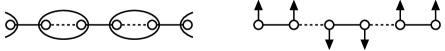
Figure 2: Physical pictures of the SD (left) and UUDD (right) states. Open circles denote $S\!=\!1/2$ spins, and solid and dotted lines denote ferromagnetic and antiferromagnetic bonds, respectively. Ellipses represent singlet pairs of two $S\!=\!1/2$ spins, while arrows denote fixed projection values of the $S\!=\!1/2$ spins. As can be seen from these figures, the SD phase is a unique gapped phase, while the UUDD phase is a doubly degenerate gapped phase.

Let us now discuss how to determine numerically the phase boundary lines in the phase diagram shown in Fig. 1. We denote, respectively, by $E_{0}^{\rm P}(N,M)$ and $E_{1}^{\rm P}(N,M)$, the lowest and second-lowest energy eigenvalues of the Hamiltonian ${\cal H}$ under periodic boundary conditions within the subspace of fixed $N$ and $M$, where $M(=\!0,\pm 1,\cdots,\pm N/2)$ is the total magnetization. Furthermore, we denote by $E_{0}^{\rm T}(N,M,P)$ the lowest eigenvalue of ${\cal H}$ under twisted boundary conditions within the subspace of fixed $N$, $M$, and $P$, where $P(=\!\pm 1)$ is the eigenvalue of the space inversion operator with respect to the twisted bond. We have numerically calculated these energies for finite-size systems with up to $N\!=\!28$ spins by means of the exact-diagonalization method. The ground-state energy of the finite-$N$ system is given by $E_{0}^{\rm P}(N,N/2)$ in the F phase and by $E_{0}^{\rm P}(N,0)$ in the other phases. In the following way, we have estimated the finite-size critical values of the interaction parameters for each phase transition. Then, the phase boundary line for the transition has been obtained by connecting the results for the $N\!\to\!\infty$ extrapolation of the finite-size critical values.

First, the phase transition between the $XY$1 and SD phases is the Berezinskii-Kosterlitz-Thouless (BKT) transition[13, 14]. It is known that for this transition, the level spectroscopy method developed by Nomura and Kitazawa[16] is very powerful for calculating the phase transition line. This method implies that the finite-size critical values are estimated from

$$\Delta E_{0}^{\rm P}(N,2)=\Delta E_{0}^{\rm T}(N,0,-1),$$ (2)

under the condition that $\Delta E_{0}^{\rm T}(N,0,+1)$ is larger than these excitations, where $\Delta E_{0}^{\rm P}(N,M)=E_{0}^{\rm P}(N,M)-E_{0}^{\rm P}(N,0)$ and $\Delta E_{0}^{\rm T}(N,M,P)=E_{0}^{\rm T}(N,M,P)-E_{0}^{\rm P}(N,0)$. This equation is also applicable to estimate the nTLL-UUDD phase transition line (see Appendix). Secondly, the phase transition between the SD and UUDD phases is the 2D Ising-type transition. Therefore, as is well known, the phase transition line is determined by the phenomenological renormalization-group (PRG) method[17]. Then, to estimate the finite-size critical values, we solve the PRG equation,

$$N\,\Delta E_{1}^{\rm P}(N,0)=(N+4)\,\Delta E_{1}^{\rm P}(N+4,0)\,,$$ (3)

where $\Delta E_{1}^{\rm P}(N,M)\equiv E_{1}^{\rm P}(N,M)-E_{0}^{\rm P}(N,M)$. Thirdly, as for the phase transition between the nTLL and $XY$1 phases, the nTLL state accompanies two-magnon bound-states, while the $XY$1 state does not. Therefore, in the ground-state magnetization curve for the finite-size system, the magnetization increases from $M\!=\!0$ to $M\!=\!2$ in the former state and from $M\!=\!0$ to $M\!=\!1$ in the latter state. Thus, the finite-size critical values are estimated from

$$\Delta E_{0}^{\rm P}(N,2)=2\,\Delta E_{0}^{\rm P}(N,1)\,.$$ (4)

We note that the binding energy of two magnons[12] is defined by $E_{\rm bind}(N)\!\equiv\!\Delta E_{0}^{\rm P}(N,2)\!-\!2\,\Delta E_{0}^{\rm P}(N,1)$. Accordingly, Eq.(4) is also the condition of $E_{\rm bind}(N)\!=\!0$. Lastly, it is apparent that the finite-size critical values for the phase transitions between the F phase and one of the $XY$1 and nTLL phases are estimated from

$$E_{0}^{\rm P}(N,N/2)\!=\!E_{0}^{\rm P}(N,0)\,.$$ (5)

3 Perturbation Theory

In the nTLL phase, the important states of two $S\!=\!1/2$ spins connected by the Ising-like ferromagnetic coupling $J_{\rm F}$ are $|\uparrow\uparrow\rangle$ and $|\downarrow\downarrow\rangle$, and the remaining two states $|(1/\sqrt{2})(\uparrow\downarrow\pm\downarrow\uparrow)\rangle$ have higher energies. To describe the nTLL state, we introduce a pseudo-spin operator $T$ with $T\!=\!1/2$, where $|T^{z}=1/2\rangle=|\uparrow\uparrow\rangle$ and $|T^{z}=-1/2\rangle=|\downarrow\downarrow\rangle$. We perturbationally derive the effective Hamiltonian $\cal H_{\rm eff}$ described by $T$. We take the first term of the right-hand side of Eq.(1) as the unperturbed Hamiltonian, and the second term as the perturbation. Up to the second order perturbation calculation, we obtain the following $XXZ$ model, apart from the energy shift,

$${\cal H}_{\rm eff}=\sum_{j=1}^{N/2}\left\{J_{\rm eff}^{\perp}(T_{j}^{x}T_{j+1}^{x}+T_{j}^{y}T_{j+1}^{y})+J_{\rm eff}^{z}T_{j}^{z}T_{j+1}^{z}\right\}$$ (6)

with

$$J_{\rm eff}^{\perp}=c_{1}-2c_{2}+c_{3},~{}~{}~{}~{}~{}J_{\rm eff}^{z}=b+c_{1}+2c_{2}+c_{3},$$ (7)

$$b=J_{\rm AF}\Delta_{\rm AF},~{}~{}~{}~{}~{}c_{1}={J_{\rm AF}^{2}\over 8J_{\rm F}(1-\Gamma_{\rm F})},~{}~{}~{}~{}~{}c_{2}={J_{\rm AF}^{2}\over 8J_{\rm F}},~{}~{}~{}~{}~{}c_{3}={J_{\rm AF}^{2}\over 8J_{\rm F}(1+\Gamma_{\rm F})},$$ (8)

where $J_{\rm eff}^{\perp}\geq 0$. The very well known exact solution[14] for Eq. (6) shows that the ground state phase diagram of ${\cal H}_{\rm eff}$ consists of the F phase, the TLL phase, and the Néel phase. These phases correspond, respectively, to the F phase, the nTLL phase and the UUDD phase of the original model (1). Thus, the F-nTLL boundary line of the original model (1) is determined by $J_{\rm eff}^{z}=-J_{\rm eff}^{\perp}$, while the nTLL-UUDD boundary line by $J_{\rm eff}^{z}=J_{\rm eff}^{\perp}$. We note that the same effective Hamiltonian with the periodic boundary condition is obtained irrespective of the periodic boundary condition or the twisted boundary condition of the original Hamiltonian (1).

The nTLL-$XY1$ boundary can be estimated by considering the energy cost of replacing a $|T^{z}=\pm 1/2\rangle$ pseudo-spin in the ${\cal H}_{\rm eff}$ picture by $|(1/\sqrt{2})(\uparrow\downarrow+\downarrow\uparrow)\rangle$. If this energy cost is negative, a macroscopic number of spin pair states with $|(1/\sqrt{2})(\uparrow\downarrow+\downarrow\uparrow)\rangle$ are generated, which brings about the breakdown of the ${\cal H}_{\rm eff}$ picture. On the other hand, if this energy cost is positive, the $|(1/\sqrt{2})(\uparrow\downarrow+\downarrow\uparrow)\rangle$ spin pair state are scarcely yielded, resulting in the stability of the ${\cal H}_{\rm eff}$ picture. The replacement of a pseudo-spin $|T^{z}=-1/2\rangle\Rightarrow|(1/\sqrt{2})(\uparrow\downarrow+\downarrow\uparrow)\rangle$ in the $M=0$ ground state leads to the $M=1$ state. Thus, if this cost is positive, the $M=1$ excitation is gapped, which is consistent with the picture of the nTLL state. We note that the replacement of a $|T^{z}=-1/2\rangle$ spin state by a $|T^{z}=+1/2\rangle$ one brings about the $M=2$ state. After some calculations, we obtain this energy cost as $(1/2)\{J_{\rm F}(1-\Gamma_{\rm F})-J_{\rm AF}\}$. Thus, the nTLL-$XY1$ boundary line is estimated by $J_{\rm AF}=J_{\rm F}(1-\Gamma_{\rm F})$.

The above three boundary lines are depicted in Figs. 1(a”), (b”), and (c”).

4 Concluding Remarks

We have determined the ground-state phase diagram of the $S\!=\!1/2$ ferromagnetic-antiferromagnetic bond-alternating chain described by the Hamiltonian of Eq. (1) by using mainly the numerical methods. Discussing the case where the ferromagnetic interactions with the Ising-type anisotropy are much stronger than the antiferromagnetic ones with the $XY$-type anisotropy, we have shown that in the phase diagrams (see Fig. 1), there appear the F, $XY$1, SD, and UUDD phases as well as the nTLL phase. We have also developed the perturbation theory, which qualitatively explains the numerically obtained phase boundary lines associated with the nTLL phase. This paper gives, in a succession of our previous work[12], a report of the appearance of the nTLL phase in an unfrustrated $S\!=\!1/2$ chain under no external magnetic field.

It should be noted that the SDW₂[3] (’SDW’ is an abbreviation for ’spin-density-wave’) does not appear in the ground-state phase diagram of the present model. The reason for this is as follows. In both of the nTLL state and the SDW₂ state, both of the nematic four-spin correlation $C_{2}(j)\equiv\langle S_{1}^{+}S_{2}^{+}S_{1+j}^{-}S_{2+j}^{-}\rangle$ and the longitudinal two-spin correlation $C_{z}(j)\equiv\langle S_{1}^{z}S_{1+j}^{z}\rangle$, where $j$ is even, decay in power laws. The former correlation is dominant in the nTLL state, while the latter is dominant in the SDW₂ state. Namely, $\eta_{2}<\eta_{z}$ in the nTLL state, whereas $\eta_{2}>\eta_{z}$ in the SDW₂ state, where $\eta_{2}$ and $\eta_{z}$ are the power-decay exponents of $C_{2}(j)$ and $C_{z}(j)$, respectively. Since there is the TLL relation $\eta_{2}\eta_{z}=1$, it holds $\eta_{2}>1$ in the SDW₂ state. However, this condition $\eta_{2}>1$ is nothing but the necessary condition for the UUDD state (see Appendix). In the zero magnetization case, the operator coming from the Umklapp process becomes relevant due to $\eta_{2}>1$, which leads to the UUDD state. Thus, the SDW₂ region does not exist in the ground state phase diagram. On the other hand, in the finite magnetization case, since the operator induced by the Umklapp process does not exist, the SDW₂ region appears in the phase diagram.

One can see several tricritical points in the phase diagrams given in Fig. 1; these are the F-$XY$1-nTLL, $XY$1-SD-UUDD, and $XY$1-UUDD-nTLL tricritical points in the case (a), the F-$XY$1-nTLL, $XY$1-SD-nTLL, and SD-UUDD-nTLL tricritical points in the case (b), and the SD-UUDD-nTLL and $XY$1-SD-nTLL tricritical points in the case (c). According to the discussion on the university class (see Appendix), on the other hand, two tricritical points associated with the $XY$1, SD, UUDD, and nTLL phases should merge into one $XY$1-SD-UUDD-nTLL tetracritical point. In order to obtain numerically this tetracritical point, it is indispensable to develop a new numerical method which is applicable commonly to the phase transition between the $XY1$ and nTLL phases and to that between the SD and UUDD phase. Since both of these transitions are of the 2D Ising-type, it seems not to be impossible to find this method. However, it is has not yet been succeeded at present, and thus this problem is beyond the scope of the present study. Furthermore, it may be expected that the nTLL phase appear even in the case where the antiferromagnetic interactions are stronger than the ferromagnetic interactions in the ground-state phase diagram of the present system, if $1.0\gg\Gamma_{{\rm F}}\!\geq\!0.0.$ and $1.0\gg|\Delta_{{\rm AF}}|$. We are now planning to perform this calculation, and the results will be reported in the near future.

Appendix A The Level Spectroscopy Method for the nTLL-UUDD Transition

Let us consider the transverse two-spin correlation $C_{1}(j)\equiv\langle S_{1}^{+}S_{1+j}^{-}\rangle$ and the nematic four-spin correlation $C_{2}(j)\equiv\langle S_{1}^{+}S_{2}^{+}S_{1+j}^{-}S_{2+j}^{-}\rangle$, where $j$ is even. Both of them decay in power laws in the $XY1$ phase with the relation $\eta_{2}=4\eta_{1}$ [12], where $\eta_{1}$ and $\eta_{2}$ are the power-decay exponents of $C_{1}(j)$ and $C_{2}(j)$, respectively. As is well known, the BKT transition from the $XY1$ phase to the unique gapped phase (the SD phase in the present case) occurs at $\eta_{1}=1/4$ (hence $\eta_{2}=1$), whereas to the doubly degenerate gapped phase (the UUDD phase in the present case) at $\eta_{1}=1$ (accordingly $\eta_{2}=4$) [15, 16]. In the level spectroscopy method by Nomura and Kitazawa[16] for the BKT transition between the $XY1$ phase and the SD phase, we search the $\eta_{2}=1$ line. This is clear from the fact that the excitation $\Delta E_{0}^{\rm P}(N,2)$ is used in Eq.(2), since $\Delta E_{0}^{\rm P}(N,2)$ is closely related to $\eta_{2}$ as $\eta_{2}=\lim_{N\to\infty}[N\Delta E_{0}^{\rm P}(N,2)/\pi v_{\rm s}]$, where $v_{\rm s}$ is the spin wave velocity [15, 16, 18, 19].

On the other hand, in the nTLL phase, $C_{1}(j)$ exhibits the exponential decay, while $C_{2}(j)$ the power decay. Thus, the role of $\eta_{1}$ in the BKT transitions from the $XY1$ phase is superseded by $\eta_{2}$ in those from the nTLL phase. Namely, the BKT transition from the nTLL phase to the unique gapped phase occurs at $\eta_{2}=1/4$, while that to the doubly degenerate gapped state at $\eta_{2}=1$. Hence, the BKT transition from the nTLL phase to the doubly degenerate gapped phase (the UUDD phase in the present case) can also be determined by Eq.(2) in which the line $\eta_{2}=1$ is searched.

Neither the BKT transition from the $XY1$ phase to the UUDD phase nor that from the nTLL phase to the SD phase occurs on the $\eta_{2}=1$ line. This is because the former transition should occur at $\eta_{1}=1$ ($\eta_{2}=4$) even if it occurs. Similarly the latter should occur at $\eta_{2}=1/4$ even if it occurs. Accordingly there should exist the $XY$1-SD-UUDD-nTLL tetracritical point on the $\eta_{2}=1$ line which is determined by Eq.(2). A similar discussion can also be applied to the $S\!=\!1$ chain with the XXZ and on-site anisotropies which has been discussed, for example, by Chen et al. [20]. Namely, the $XY$1-Haldane-Néel-nTLL tetracritical point should exist in this $S\!=\!1$ chain.

References

- [1] A. V. Chubukov, Phys. Rev. B 44, 4693 (1991).
- [2] T. Vekua, A. Honecker, H.-J. Mikeska and F. Heidrich-Meisner, Phys. Rev. B 76, 174420 (2007).
- [3] T. Hikihara, L. Kecke, T. Momoi and A. Furusaki, Phys. Rev. B 78, 144404 (2008).
- [4] J. Sudan, A. Lüscher and A. M. Läuchli, Phys. Rev. B 80, 140402(R) (2009).
- [5] T. Sakai, T. Tonegawa and K. Okamoto, Phys. Status Solidi B 247, 583 (2010).
- [6] M. Sato, T. Hikihara and T. Momoi, Phys. Rev. Lett. 110, 077206 (2013).
- [7] O. A. Starykh and L. Balents, Phys. Rev. B 89, 104407 (2014).
- [8] N. Büttgen, K. Nawa, T. Fujita, M. Hagiwara, P. Kuhns, A. Prokofiev, A. P. Reyes, L. E. Svistov, K. Yoshimura and M. Takigawa, Phys. Rev. B 90, 134401 (2014).
- [9] A. Orlova, E. L. Green, J. M. Law, D. I. Gorbunov, G. Chanda, S. Krämer, M. Horvatić, R. K. Kremer, J. Wosnitza and G. L. J. A. Rikken, Phys. Rev. Lett. 118, 247201 (2017).
- [10] A. Parvej and M. Kumar, Phys. Rev. B 96, 054413 (2017).
- [11] M. Bosioc̆ić, F. Bert, S. E. Dutton, R. J. Cava, P. J. Baker, M. Poz̆ek and P. Mendels, Phys. Rev. B 96, 224424 (2017).
- [12] T. Tonegawa, T. Hikihara, K. Okamoto, S. C. Furuya and T. Sakai, J. Phys. Soc. Jpn. 87, 104002 (2018).
- [13] Z. L. Berezinskii, Sov. Phys. JETP 34, 610 (1971); J. M. Kosterlitz and D. J. Thouless, J. Phys. C 6, 1181 (1973).
- [14] T. Giamarchi, Quantum Physics in One Dimension (Clarendon Press, Oxford, 2003).
- [15] A. Kitazawa, K. Nomura and K. Okamoto, Phys. Rev. Lett. 76, 4038 (1996).
- [16] K. Nomura and A. Kitazawa, J. Phys. A 31, 7341 (1998).
- [17] M. P. Nightingale, Physica A 83, 561 (1976).
- [18] J. L. Cardy, J. Phys. A: Math. Gen. 17, L385 (1984).
- [19] T. Sakai, Phys. Rev. B 58, 6268 (1998).
- [20] W. Chen, K. Hida and B. C. Sanctuary, Phys. Rev.B 67, 104401 (2003).