Beta-Sorted Portfolios

Abstract

Beta-sorted portfolios—portfolios comprised of assets with similar covariation to selected risk factors—are a popular tool in empirical finance to analyze models of (conditional) expected returns. Despite their widespread use, little is known of their statistical properties in contrast to comparable procedures such as two-pass regressions. We formally investigate the properties of beta-sorted portfolio returns by casting the procedure as a two-step nonparametric estimator with a nonparametric first step and a beta-adaptive portfolios construction. Our framework rationalizes the well-known estimation algorithm with precise economic and statistical assumptions on the general data generating process. We provide conditions that ensure consistency and asymptotic normality along with new uniform inference procedures allowing for uncertainty quantification and general hypothesis testing for financial applications. We show that the rate of convergence of the estimator is non-uniform and depends on the beta value of interest. We also show that the widely-used Fama-MacBeth variance estimator is asymptotically valid but is conservative in general, and can be very conservative in empirically-relevant settings. We propose a new variance estimator which is always consistent and provide an empirical implementation which produces valid inference. In our empirical application we introduce a novel risk factor – a measure of the business credit cycle – and show that it is strongly predictive of both the cross-section and time-series behavior of U.S. stock returns.

Keywords: Beta pricing models, portfolio sorting, nonparametric estimation, partitioning, kernel regression, smoothly-varying coefficients.

1 Introduction

Deconstructing expected returns into idiosyncratic factor loadings and corresponding prices of risk for interpretable factors is an evergreen pursuit in the empirical finance literature. When factors are observable, there are two workhorse approaches that continue to enjoy widespread use. The first approach, Fama-MacBeth two-pass regressions, have been extensively studied in the financial econometrics literature. The second approach, which we refer to as beta-sorted portfolios, has received scant attention in the econometrics literature despite its empirical popularity.

Beta-sorted portfolios are commonly characterized by the following two-step procedure, which incorporates beta-adaptive portfolios construction. In a first step, time-varying risk factor exposures are estimated through (backwards-looking) weighted time-series regressions of asset returns on the observed factors. The most popular implementation uses rolling window regressions, often with a choice of a five-year window. In a second step, the estimated factor exposures, based on data up to the previous period, are ordered and used to group assets into portfolios. These portfolios then represent assets with a similar degree of exposure to the risk factors, and the degree of return differential for differently exposed assets is used to assess the compensation for bearing this common risk. Most frequently this is achieved by differencing the portfolio returns from the two most extreme portfolios. Finally, an average over time of these return differentials is taken to infer whether the risk is priced unconditionally—whether the portfolio earns systematic (and significant) excess returns. Notwithstanding the simple and intuitive nature of the methodology, little is known of the formal properties of this estimator and its associated inference procedures.

We provide a comprehensive framework to study the economic and statistical properties of beta-sorted portfolios. We first translate the two-step estimation algorithm with beta-adaptive portfolio construction into a corresponding statistical model. We show that the model has key features which are important to consider for valid interpretation of the empirical results. For example, in this setup, no-arbitrage conditions are not imposed and instead imply testable hypotheses. Within this framework, we introduce general sampling assumptions allowing for smoothly-varying factor loadings, persistent (possibly nonstationary) factors, and conditional heteroskedasticity across time and assets. We then study the asymptotic properties of the beta-sorted portfolio estimator and associated test statistics in settings with large cross-sectional and time-series sample sizes (i.e., $n,T\to\infty$).

We provide a host of new methodological and theoretical results. First, we introduce conditions that ensure consistency and asymptotic normality of the full-sample estimator of average expected returns. Importantly, we characterize precise conditions on the bandwidth sequence of the first-stage kernel regression estimator, $h$, and the number of portfolios, $J$, relative to growth in $n$ and $T$. We show that the rate of convergence of the estimator depends on the value of beta that is chosen. For beta values closer to zero the rate of convergence is faster and is slower otherwise; in fact, for values of beta away from zero we show that the rate of convergence of the estimator is only $\sqrt{T}$, despite an effective sample size of the order $nT$, reflecting specific properties of the setting of interest. However, we also show that certain features of average expected returns such as the discrete second derivative—which represents a butterfly spread trade—can be estimated with higher precision through faster rates of convergence for all values of beta, namely, $\sqrt{nT/J}$ for a single risk factor. This result also accommodates more powerful tests for testing the null hypothesis of no-arbitrage. Finally, we also provide novel results on uniform inference for the beta-sorted portfolio estimator for both a single period and the grand mean. This facilitates the construction of uniform confidence bands which allows for inference on a variety of hypotheses of interest such as monotonicity or inference on maximum-return trading strategies.

We also uncover some limitations of current empirical practice employing beta-sorted portfolios methodology. First, as with all nonparametric estimators, the choice of tuning parameters, $h$ and $J$, are key to successful performance and are dependent on the sample sizes $n$ and $T$. In contrast, empirical practice often chooses window length in the first step and total portfolios in the second step irrespective of the sample size at hand. Second, we show that the widely-used Fama and MacBeth (1973) variance estimator, is not consistent in general but only when conditional expected returns are constant over time for a fixed beta. However, we show that the Fama-MacBeth variance estimator still leads to valid, albeit possibly conservative, inferences. Unfortunately, in empirically-relevant settings it appears that the Fama-MacBeth variance estimator can be very conservative. To address this limitation, we propose a new variance estimator which is always consistent and provide an empirical implementation which produces valid inference. In our empirical application we show that our new variance estimator provides much sharper inference than the Fama-MacBeth variance estimator. We also show that differential returns for a single time period, often used as inputs for assessing the time-series properties of conditional expected returns, are contaminated by an additional term when risk factors are serially correlated.

From a theoretical perspective, beta-sorted portfolios present a number of technical challenges originating from the two-step estimation algorithm with beta-adaptive portfolio construction, since it relies on two nested nonparametric estimation steps together with a portfolio construction based on a first-step nonparametric generated regressor. More precisely, the first-stage nonparametrically estimated factor loadings enter directly into the (non-smooth) partitioning scheme further complicating the analysis. To our knowledge, we are the first to prove validity of such an approach.

This paper is most related to the large literature studying asset pricing models with observable factors. Given our focus on conditional asset pricing models with large panels in both the cross-section and time-series dimension, this paper is most closely related to Gagliardini, Ossola, and Scaillet (2016) (see also Gagliardini, Ossola, and Scaillet, 2020). Gagliardini, Ossola, and Scaillet (2016) introduce a general framework and econometric methodology for inference in large-dimensional conditional factors under no-arbitrage restrictions. They allow for risk exposures, which are parametric functions of observable variables and provide conditions to consistently estimate, and conduct inference on the prices of risk. Although the statistical model under study shares important similarities with the setup of Gagliardini, Ossola, and Scaillet (2016), there are substantial differences, and the models explored previously in the literature do not nest our setup. For example, the classical beta-sorted portfolio estimator implies a data-generating process that does not (necessarily) exclude arbitrage opportunities and supposes risk exposures which are smoothly-varying. Furthermore, we show that valid estimation and inference can be achieved without requiring an assumption of the functional form of the conditional expectation of the risk factors. See Section 2 for more details.

Our paper is also related to the financial econometrics literature on nonparametric estimation and inference. In particular, the two steps of the beta-sorted portfolio algorithm align individually with Ang and Kristensen (2012), who study kernel regression estimators of time-varying alphas and betas, and Cattaneo, Crump, Farrell, and Schaumburg (2020) who study portfolio sorting estimators given observed individual characteristic variables. However, the linkage between the two steps, including the role of the generated (nonparametrically estimated) regressor in the second-stage nonparametric partitioning estimator has not been studied before. Finally, our paper is also related to Raponi, Robotti, and Zaffaroni (2020) who study estimation and inference of the ex-post risk premia. In analogy, we show that estimation and inference in our general setting are sensitive to the specific object of interest chosen. For example, we show that a faster convergence rate of the estimator can be obtained by centering at realized systematic returns rather than conditional expected returns. See Section 4 for more details.

In our empirical application we introduce a novel risk factor – a measure of the business credit cycle – and show that it is strongly predictive of both the cross-section and time-series behavior of U.S. stock returns. Moreover, we show the effectiveness of our new variance estimator as inference is much sharper relative to the Fama-MacBeth variance estimator.

This paper is organized as follows. In Section 2, we introduce our general data-generating process and show how it rationalizes the two-step algorithm used to construct beta-sorted portfolios. In Section 3, we study the theoretical properties of the first-step estimators of the time-varying risk factor exposures. Using these results, in Section 4 we establish the theoretical properties of the second-step nonparametric estimator. To facilitate feasible inference, Section 5 introduces pointwise and uniform inference procedures for the grand-mean estimator including characterizing the properties of the commonly-used Fama-MacBeth variance estimator. Section 6 presents an empirical application, and Section 7 concludes. Detailed assumptions and proofs of the results are relegated to a Supplemental Appendix (hereafter, SA).

Notation and conventions

It is useful to introduce the following notation. For a constant $k\in N$ and a vector $v=(v_{1},\ldots,v_{d})^{\top}\in\mathbb{R}^{d},$ we denote $|v|_{k}=(\sum_{i=1}^{d}|v_{i}|^{k})^{1/k}$, $|v|=|v|_{2}$ and $|v|_{\infty}=\max_{i\leq d}|v_{i}|$. For a matrix $A=(a_{ij})_{1\leq i\leq m,1\leq j\leq n}$, we define the spectral norm $|A|_{2}=\max_{|v|=1}|Av|$, the max norm $|A|_{\max}=\max_{1\leq i\leq m,1\leq j\leq n}|a_{i,j}|$, $|A|_{1}=\max_{1\leq j\leq n}\sum_{i=1}^{m}a_{i,j}$, and $|A|_{\infty}=\max_{1\leq i\leq m}\sum_{j=1}^{n}a_{i,j}$. For a function $f,$ we denote $|f|_{\infty}=\sup_{x\in\mathcal{X}}|f(x)|$, where $\mathcal{X}$ denotes the support. We set $(a_{n}:n\geq 1)$ and $(b_{n}:n\geq 1)$ to be positive number sequences. We write $a_{n}=\textit{O}(b_{n})$ or $a_{n}\lesssim b_{n}$ (resp. $a_{n}\asymp b_{n}$) if there exists a positive constant $C$ such that $a_{n}/b_{n}\leq C$ (resp. $1/C\leq a_{n}/b_{n}\leq C$) for all large $n$, and we denote $a_{n}=\textit{o}(b_{n})$ (resp. $a_{n}\sim b_{n}$), if $a_{n}/b_{n}\to 0$ (resp. $a_{n}/b_{n}\to C$). Limits are taken as $n,T\to\infty$ unless otherwise stated explicitly. $\mbox{plim}X_{n}=X$ means that $X_{n}\to_{\mathbb{P}}X$. $\to_{\mathcal{L}}$ denotes convergence in law. Define $X_{n}=O_{\mathbb{P}}(a_{n}):\mbox{lim}_{n\to\infty}\mathbb{P}(|X_{n}|\geq\delta_{\varepsilon}a_{n})\to 0\quad\forall\varepsilon>0$. Define $X_{n}=o_{\mathbb{P}}(a_{n}):\forall\varepsilon,\delta>0\quad\exists N_{\varepsilon,\delta}\quad\text{ such that }\mathbb{P}(|X_{n}|\geq\delta a_{n})\leq\varepsilon\quad\forall n>N_{\varepsilon,\delta}$. Let $X_{n}\lesssim_{\mathbb{P}}a_{n}$ means $X_{n}=O_{\mathbb{P}}(a_{n})$.

2 Model setup

We introduce a general statistical model of asset returns and show how the proposed model naturally aligns with the two steps that comprise the beta-sorted portfolio algorithm. We discuss the relevant properties of the model especially with respect to the potential presence of arbitrage opportunities.

2.1 Modeling returns

Let $R_{it}$ denote the return of asset $i$ at time $t$. We assume that asset returns are generated by the linear stochastic coefficient model,

$$R_{it}=\alpha_{it}+\beta_{it}^{\top}f_{t}+\varepsilon_{it},\qquad i=1,\cdots,n_{t},\qquad t=1,\cdots,T,$$ (2.1)

where $\alpha_{it}\in\mathbb{R}$ and $\beta_{it}\in\mathbb{R}^{d}$ ($d\geq 1$) are random coefficients which are measurable to a filtration based on the past information, $f_{t}$ is a vector of observable risk factors, and $\varepsilon_{it}$ is an idiosyncratic error term. We allow for an unbalanced panel, but assume that $n\leq n_{t}\leq n_{u}$ and $n\asymp n_{u}$, so that each cross-section contributes to the asymptotic properties of the estimator.

We define the filtration $\mathcal{F}_{n,T,t-1}=\sigma((\alpha_{it})^{n_{t},t}_{i=1,t=1},(\beta_{it})^{n_{t},t}_{i=1,t=1},(f_{t})^{t-1}_{t=1},(\varepsilon_{it})_{i=1,t=1}^{n_{t},t-1})$. Hereafter, we suppress the $n$ and $T$ as in $\mathcal{F}_{n,T,t-1}$ and denote it as $\mathcal{F}_{t-1}$ for simplicity of notation. We define another cross-sectional invariant filtration $\mathcal{G}_{t-1}$. Suppose that $\beta_{it}=G_{\beta}(\eta_{i},g_{1},\cdots,g_{t-1},f_{1},\cdots,f_{t-1},\omega_{it})$, where $\eta_{i}$ is independent and identically distributed (i.i.d.) over $i$, $g_{t}$ are i.i.d. factors over $t$, and $\omega_{it}$ are i.i.d. over $t$ and $i$. Then, the cross-section invariant sigma field is $\mathcal{G}_{t}=\sigma(f_{1},\cdots,f_{t},g_{1},\cdots,g_{t})$. This setup may appear restrictive but is in fact general: we can always increase the dimension of the random variables entering the sigma field to accommodate more complex designs. Consequently, without loss of generality, we assume $\mathbb{E}(f_{t}|\mathcal{G}_{t-1})=\mathbb{E}(f_{t}|\mathcal{F}_{t-1})$.

To obtain the structural form of our model, we denote $\mu_{t}(\beta)$ as the conditional expected return of an asset with risk exposure $\beta$. Thus,

$$\mathbb{E}(R_{it}|\mathcal{F}_{t-1})=\mu_{t}(\beta_{it}),$$ (2.2)

so that using equation (2.1) we have,

$$\mu_{t}(\beta_{it})=\alpha_{it}+\beta_{it}^{\top}\mathbb{E}(f_{t}|\mathcal{F}_{t-1}).$$ (2.3)

Finally, combining equations (2.1) and (2.3), we obtain the structural form

$$R_{it}=\mu_{t}(\beta_{it})+\beta_{it}^{\top}(f_{t}-\mathbb{E}[f_{t}|\mathcal{F}_{t-1}])+\varepsilon_{it}.$$ (2.4)

To distinguish conditional expected returns, $\mu_{t}(\beta_{it})$, from systematic realized returns, we define

$${M}_{t}(\beta_{it})=\mu_{t}(\beta_{it})+\beta_{it}^{\top}(f_{t}-\mathbb{E}[f_{t}|\mathcal{F}_{t-1}])=\alpha_{it}+\beta_{it}^{\top}f_{t}$$

to represent the latter object.

Equation (2.4) may be compared to the standard beta pricing model (e.g., Cochrane, 2005, Chapter 12) and generalizations thereof (e.g., Cochrane, 1996; Adrian, Crump, and Moench, 2015; Gagliardini, Ossola, and Scaillet, 2016). The most noteworthy difference between equation (2.4) is the presence of the (possibly) nonlinear, time-varying function $\mu_{t}\left(\beta_{it}\right)$. When $R_{it}$ represent excess returns then the no-arbitrage restriction implies that $\mu_{t}\left(\beta_{it}\right)=\beta_{it}^{\top}\lambda_{t}$ for some $\lambda_{t}$ (Gagliardini, Ossola, and Scaillet, 2016). Our model nests, but does not require, the imposition of the absence of arbitrage opportunities so that

$$R_{it} =\mu_{t}(\beta_{it})+\beta_{it}^{\top}(f_{t}-\mathbb{E}[f_{t}|\mathcal{F}_{t-1}])+\varepsilon_{it},$$

$$=\underset{\text{deviation from no-arbitrage}}{\underbrace{\big{(}\mu_{t}(\beta_{it})-\beta_{it}^{\top}\lambda_{t})}}+\beta_{it}^{\top}\lambda_{t}+\beta_{it}^{\top}(f_{t}-\mathbb{E}[f_{t}|\mathcal{F}_{t-1}])+\varepsilon_{it}.$$

The presence of this additional term representing the deviation from no-arbitrage restrictions can be motivated by appealing to structural models which feature violations of the law of one price. Such a setup as in equation (2.4) could arise, for example, in the margin-constraints model of Garleanu and Pedersen (2011) under the assumption that the security’s margin is a nonlinear function of its past beta.

To see why equation (2.4) rationalizes the beta-sorted portfolio algorithm, consider the two steps in the case when $d=1$.

Step 1: Estimation of $\alpha_{it}$ and $\beta_{it}$.

For each individual asset, we calculate the local constant estimator for $\alpha_{it}$ and $\beta_{it}$ as,

$$\left(\widehat{\alpha}_{it_{0}},\widehat{\beta}_{it_{0}}\right)^{\top}=\Big{(}\sum^{t_{0}-1}_{t=1}K((t-t_{0})/(Th))X_{t}X_{t}^{\top}\Big{)}^{-1}\Big{(}\sum^{t_{0}-1}_{t=1}K((t-t_{0})/(Th))X_{t}R_{it}\Big{)},$$ (2.5)

where $X_{t}=(1,f_{t})^{\top}$, $K(\cdot)$ is a kernel function and $h$ a positive bandwidth determining the length of the rolling window. This construction purposely does not have “look-ahead bias”; moreover, the estimators $\widehat{\alpha}_{it_{0}}$ and $\widehat{\beta}_{it_{0}}$ do not use data from time $t_{0}$ in their construction (a “leave-one-out” estimator). This estimation of the time-varying random coefficients can be interpreted as a kernel regression of equation (2.1) for each cross-section unit. When $K(\cdot)$ takes on a constant value for the most recent prior $H$ time periods, and zero otherwise, we obtain the familiar rolling window regression estimator with window size $H$. $\blacksquare$

Step 2: Sorting portfolios using estimated $\beta_{it}$.

To see that this comprises cross-sectional nonparametric estimation observe that, for fixed $t$, Equation (2.2) is the conditional mean of interest. We define $\mathcal{B=}[\beta_{l},\beta_{u}]$ as the support of the possible realizations of $\beta_{it}$ across $i$ and $t$. For each $t=1,\ldots,T$, let us define a beta-adaptive partition of this support as

$$\widehat{P}_{jt}=[\widehat{\beta}_{(\lfloor n_{t}(j-1)/J_{t}\rfloor)t},\widehat{\beta}_{(\lfloor n_{t}j/J_{t}\rfloor)t}),\qquad\qquad j=1,\ldots J_{t}-1$$

$$\widehat{P}_{jt}=[\widehat{\beta}_{(\lfloor n_{t}(J-1)/J\rfloor)t},\widehat{\beta}_{(n_{t})t}],\qquad\qquad j=J_{t},$$

where $\lfloor.\rfloor$ denotes the floor function and $\widehat{\beta}_{(\ell)t}$ denotes the $\ell$th order statistic of the estimated betas in the first step across $i$ for fixed $t$, i.e., the order statistics of $\{\widehat{\beta}_{it}:i=1,\ldots,n_{t}\}$. The number of portfolios $J_{t}$, and their random structure (i.e., break-point positions based on estimated $\beta_{it}$), vary for each time period. Then, define

$$\widehat{p}_{jt}(\beta)=\mathbf{1}\{\beta\in\widehat{P}_{jt}\},$$

with $\mathbf{1}\{\cdot\}$ the indicator function, and $\widehat{\Phi}_{t}=[\widehat{\Phi}_{i,j,t}]_{n_{t}\times J_{t}}^{\top}$ the matrix with element $\widehat{\Phi}_{i,j,t}=\widehat{p}_{jt}(\widehat{\beta}_{it})$. We also let $\widehat{p}_{jt}(\beta)$ be $\widehat{p}_{jt}$ in later sections. We can then obtain

$$\widehat{a}_{t}=(\widehat{\Phi}_{t}{\widehat{\Phi}}_{t}^{\top})^{-1}({\widehat{\Phi}}_{t}R_{t}),$$

which represent the average returns of assets in $\widehat{P}_{jt}$ for $j=1,\ldots,J_{t}$ at time $t$. Define $\widehat{a}_{jt}$ as the $j$th element of $\hat{a}_{t}$.

Letting $\widehat{a}_{lt}$ and $\widehat{a}_{ut}$ be the portfolio returns of the two extreme portfolios, a common object of interest is the differential average returns in the most extreme portfolios:

$$\frac{1}{T}\sum_{t=1}^{T}(\widehat{a}_{ut}-\widehat{a}_{lt})=\frac{1}{T}\sum_{t=1}^{T}\Big{(}\widehat{\mu}_{t}(\beta_{u})-\widehat{\mu}_{t}(\beta_{l})\Big{)},$$

where

$$\widehat{\mu}_{t}(\beta)=\sum_{j=1}^{J_{t}}\widehat{p}_{jt}(\beta)\widehat{a}_{jt}.$$ (2.6)

More generally, many other estimators of interest in finance can be defined as transformations of the stochastic processes $(\widehat{\mu}_{t}(\beta):\beta\in\mathcal{B})$, for each cross-section.

Similarly, other estimators of interest can be considered by averaging across time. These estimators can be thought of as transformations of the stochastic process $(\widehat{\mu}(\beta):\beta\in\mathcal{B})$ with

$$\widehat{\mu}(\beta)=\frac{1}{T}\sum_{t=1}^{T}\widehat{\mu}_{t}(\beta)=\frac{1}{T}\sum_{t=1}^{T}\sum_{j=1}^{J_{t}}\widehat{p}_{jt}(\beta)\widehat{a}_{jt}.$$ (2.7)

For example, we can estimate conditional expected returns for all values of $\beta$ rather than only values near $\beta_{l}$ and $\beta_{u}$. Correspondingly, $\widehat{\mu}_{t}(\beta)$ and $\widehat{\mu}(\beta)$ may be directly interpreted as nonparametric estimators of expected returns. $\blacksquare$

A few comments are in order. First, the above two steps are completely in line with the empirical finance literature. Importantly, at no point in the two-step algorithm is the requirement to estimate the conditional expectation of the risk factors, $\mathbb{E}[f_{t}|\mathcal{F}_{t-1}]$, and so the researcher remains agnostic about the dynamics of these risk factors. We will revisit this issue in the next section. Second, the practice of moving-window regressions to accommodate time variation in $\beta_{it}$ suggests a slowly-varying coefficient model as previously used in finance applications such as in Ang and Kristensen (2012) and Adrian, Crump, and Moench (2015). However, in contrast to these previous formulations, we do not condition on the realizations of the random processes $\alpha_{it}$ and $\beta_{it}$. Instead, we retain the randomness in these objects so that the second-stage beta-sorted portfolio estimator can have a well-defined limit as $n,T\to\infty$. Third, an alternative to the smoothly-varying coefficients approach is to specify $\beta_{it}$ as a functions of individual characteristics and possibly also of economy-wide variables (see, for example, Gagliardini, Ossola, and Scaillet, 2020, and references therein). Our approach can straightforwardly accommodate such settings by modifying the kernel regressions appropriately.

Finally, the more general estimation approach described in equations (2.6) and (2.7), with more details in Section 4, does not constitute spurious generality. The conventional implementation of beta-sorted portfolios relies on a constant choice of $J_{t}=J\,\,\forall t$ and so averages $J$ portfolios across all time periods. However, if the cross-sectional distribution of the $\beta_{it}$ are changing over time then there is no guarantee that each portfolio represents assets with sufficiently similar betas. For example, it may be that assets with values of $\beta$ near $1/2$ fall in the sixth portfolio at times and the fifth portfolio at other times and so on. Thus, the conventional estimator will be, in general, both more biased and more variable than the estimators suggested in equations (2.6) and (2.7), all else equal. This is of special importance when we are interested in expected returns for intermediate values of betas and also in situations where tests of monotonicity or shape restrictions are of interest.

3 First step: rolling regressions

The first step involves a kernel regression of a linear stochastic coefficients model. Recall that $X_{t}=(1,f_{t})$ and define $b_{it}=(\alpha_{it},\beta_{it})$. Then, we can rewrite equation (2.1) as

$$R_{it_{0}}=X_{t_{0}}^{\top}b_{it_{0}}+\varepsilon_{it_{0}}.$$

We assume that $\mathbb{E}(\varepsilon_{it}|\mathcal{F}_{t-1})=\mathbb{E}{{}_{t-1}}(\varepsilon_{it})=0$ and, because $\alpha_{it}$ and $\beta_{it}$ are measurable with respect to $\mathcal{F}_{t-1}$, then $\alpha_{it_{0}}$ and $\beta_{it_{0}}$ can be identified as

$$b_{it_{0}}=\mathbb{E}(X_{t_{0}}X_{t_{0}}^{\top}|\mathcal{F}_{t_{0}-1})^{-1}\mathbb{E}(X_{t_{0}}R_{it_{0}}|\mathcal{F}_{t_{0}-1}).$$

The kernel estimator from (2.5) is then $\widehat{b}_{it_{0}}=(\widehat{\alpha}_{it_{0}},\widehat{\beta}_{it_{0}})^{\top}$. In order to accommodate the random coefficients we exploit the fact that $\sum^{t_{0}-1}_{t=1}K((t-t_{0})/(Th))X_{t}X_{t}^{\top}$ and $\sum^{t_{0}-1}_{t=1}K((t-t_{0})/(Th))X_{t}R_{it}$ are close, in the appropriate sense, to $\sum^{t_{0}-1}_{t=1}\mathbb{E}[K((t-t_{0})/(Th))X_{t}X_{t}^{\top}|\mathcal{F}_{t-1}]$ and $\sum^{t_{0}-1}_{t=1}\mathbb{E}[K((t-t_{0})/(Th))X_{t}R_{it}|\mathcal{F}_{t-1}]$, since their difference are summands of martingale difference sequences.

To formalize the intuition and establish uniform consistency and asymptotic normality of $\widehat{b}_{it_{0}}$ we require technical, but relatively standard, assumptions on the underlying data generating process. We report these assumptions in the Appendix (Assumptions 16–21) and discuss them briefly here. Assumption 16 ensures that the one-sided kernel $K(\cdot)$ satisfies standard properties such as being nonzero on a compact support and twice continuously differentiable. The one-sided kernel ensures that we do not have any look-ahead bias, so the procedure can be interpreted as real-time estimation, and also to define the appropriate conditional moments for the second step discussed in the next section. Assumption 17 imposes some structure on the time series properties of the factor $f_{t}$ but is quite general and allows for certain forms of nonstationary behavior. We could relax some of these assumptions to allow for even more complex time-series properties at the expense of more detailed notation and proofs. Assumption 17 also imposes moment conditions on the idiosyncratic error term, $\varepsilon_{it}$. Assumption 18 ensures that $b_{it_{0}}$ is well defined for all $t_{0}$. Assumptions 19 and 21 are regularity conditions on the rate of decay of the time-series dependence of the risk factors. Finally, Assumption 20 ensures that the alphas and betas, although random, are sufficiently smooth over time (i.e., satisfying a Lipschitz-type condition). Similar assumptions are generally imposed in varying coefficient models (see, for example, Zhang and Wu, 2015).

We first provide a uniform consistency results of our estimator $\widehat{b}_{it_{0}}$ over $i$ and $t$. We require this result to precisely control the effect of estimating $\beta_{it}$ in the first step when entering the second-step estimator. We establish this consistency on a compact interval of a trimmed support with trimming length $\lfloor Th\rfloor$. Let $q$ denote the parameter in Assumption 17.

Theorem 3.1.

Suppose Assumptions 16–21 hold, and let $r_{T}=(Th)^{-1}(T^{1/q}+\sqrt{Th\log T})\to 0$, $h\to 0$, and $\log(n_{u}T)/Th\to 0$. Then,

$$\max_{1\leq i\leq n}\sup_{\lfloor Th\rfloor\leq t_{0}\leq T-\lfloor Th\rfloor}\big{|}\widehat{b}_{it_{0}}-b_{it_{0}}\big{|} \lesssim_{\mathbb{P}}\delta_{T},$$

where $\delta_{T}=(r_{T}+\sqrt{\log(n_{u}T)}/\sqrt{Th}+h)$.

Theorem B.6 provides uniform rates of convergence for the first-stage kernel estimators of the betas. Naturally, these rates depend on $n$, $T$, and $h$ but are also directly dependent on $q$ which represents the number of bounded moments of the idiosyncratic error term. For very large $q$, essentially the uniformity is attained at rate only slower by a $\log(T)$ factor. Importantly, the theorem shows that we attain the same uniform rate for the leave-one-out estimator which ensures our theoretical results mimic empirical practice exactly.

Although estimation of $\mu(\cdot)$ is generally of interest, there are some situations where inference on $\beta_{it}$ directly is instead the primary goal. To introduce the necessary results we need to present some additional useful notation. To allow for a flexible class of time series processes we model the factor, $f_{t}$, as a sum of two components, $f_{t}=\tau_{t}+x_{t}$, where $\tau_{t}$ is a smoothly-varying process and $x_{t}$ is a strictly stationary process. Then we can define $\tau_{t}=\tau^{\prime}(t/T)$ for a smooth function $\tau^{\prime}:[0,1]\mapsto\mathbb{R}$. Also define, $\Sigma_{x}=\mathbb{E}[(1,x_{t})(1,x_{t})^{\top}]$, $\tilde{\tau}(t_{0}/T)=(1,\tau^{\prime}(t_{0}/T))^{\top}$. We let $\Sigma_{A}=\Sigma_{x}+\tilde{\tau}(t_{0}/T)\tilde{\tau}(t_{0}/T)^{\top}$, $\Sigma_{B}=\sigma_{\varepsilon,0}^{2}\mathbb{E}(X_{t_{0}}X^{\top}_{t_{0}})\int_{-1}^{0}K^{2}(s)ds$. $\Sigma_{b}=\Sigma_{A}^{-1}\Sigma_{B}\Sigma_{A}^{-1}=\Sigma_{A}^{-1}\sigma_{\varepsilon,0}^{2}\int_{-1}^{0}K^{2}(s)ds$. With these definitions in place, we next show asymptotic normality of our estimator $\widehat{b}_{it_{0}}$.

Theorem 3.2 (Asymptotic Normality).

Let $h\sqrt{hT}\to 0$, $h\to 0$, $Th\to\infty$, $r_{AT}+r_{T}\to 0$ then, under Assumptions 16-21, we have that

$$\sqrt{Th}\Sigma_{b}^{-1/2}\big{(}\widehat{b}_{it_{0}}-b_{it_{0}}\big{)}\to_{\mathcal{L}}\mathsf{N}(0,I).$$ (3.1)

where $r_{AT}$ is defined in the Appendix.

We show in the appendix that the limiting asymptotic distribution is invariant to whether the leave-one-out or general kernel estimator is used. The results in Theorem B.7 can to be extended to distribution results which are uniform over $t$; however, we don’t pursue this here as our main focus is on the beta-sorted estimator. Finally, note that to construct a confidence interval for ${b}_{it_{0}}$ based on $\widehat{b}_{it_{0}}$, we require a consistent estimator of the asymptotic variance of $\widehat{b}_{it_{0}}$. Using residuals from the initial step, i.e., $\widehat{\varepsilon}_{it}$, $\sigma_{t}^{2}$ can be estimated by

$$(\widehat{\sigma}^{2}_{t_{0}},\widehat{\varsigma}^{2}_{t_{0}})^{\top}=\operatorname*{arg\,min}_{c_{0},c_{1}}\sum_{t=1}^{t_{0}-1}\sum_{i=1}^{n_{t}}K\Big{(}\frac{t-t_{0}}{Th}\Big{)}\big{(}\widehat{\varepsilon}^{2}_{it}-c_{0}-c_{1}(t-t_{0})/T\big{)}^{2}.$$

So $\widehat{\Sigma}_{b}$ can be obtained by $TA(t_{0})^{-1}\widehat{\sigma}(t_{0}/T)\int_{0}^{1}K^{2}(w)dw$.

4 Second step: beta sorts

The second step of the estimation procedure is to sort assets by their value of $\widehat{\beta}_{it}$ obtained from the procedure described in the previous section. Recall that the structural form of our model is

$$R_{it} =\mu_{t}(\beta_{it})+\beta_{it}^{\top}(f_{t}-\mathbb{E}(f_{t}|\mathcal{F}_{t-1}))+\varepsilon_{it}$$

$$=M_{t}(\beta_{it})+\varepsilon_{it},$$

and under our assumptions we have $\mathbb{E}({\varepsilon}_{it}|\mathcal{F}_{t-1},\beta_{it})=\mathbb{E}({\varepsilon}_{it}|\mathcal{F}_{t-1})=0$.

To gain intuition, suppose that the $\beta_{it}$ were observed. The second equality makes clear that, for a fixed $t$, we can only nonparametrically estimate the unknown function $M_{t}(\cdot)$ rather than the direct object of interest $\mu_{t}(\cdot)$. However,

$$\frac{1}{T}\sum_{t=1}^{T}{M}_{t}(\beta)=\frac{1}{T}\sum_{t=1}^{T}\mu_{t}(\beta)+\frac{1}{T}\sum_{t=1}^{T}\beta^{\top}(f_{t}-\mathbb{E}(f_{t}|\mathcal{F}_{t-1})).$$ (4.1)

The second term has summands, $\beta^{\top}(f_{t}-\mathbb{E}(f_{t}|\mathcal{F}_{t-1}))$, which are a martingale difference sequence with respect to $\mathcal{F}_{t}$ and so we would expect this sample average to converge to zero in probability; consequently, this would ensure that $T^{-1}\sum_{t=1}^{T}{M}_{t}(\beta)$ and $T^{-1}\sum_{t=1}^{T}\mu_{t}(\beta)$ are uniformly (in $\beta$) close in probability for large $T$. A further complication, of course, is introduced by using an estimated $\beta_{it}$ in the second-stage nonparametric regression. Nevertheless, in this section, we will make these arguments rigorous and provide appropriate conditions for consistency and asymptotic normality for the beta-sorted portfolio estimator.

To motivate the assumptions we introduce shortly, note that we may rewrite our model as

$$R_{it}=\alpha_{it}+\beta_{it}^{\top}\mathbb{E}(f_{t}|\mathcal{F}_{t-1})+\tilde{\varepsilon}_{it},$$

where $\tilde{\varepsilon}_{it}=\beta_{it}^{\top}(f_{t}-\mathbb{E}(f_{t}|\mathcal{F}_{t-1}))+\varepsilon_{it}$ represents the sum of two different martingale difference sequences. This form makes clear that we require assumptions on $\alpha_{it}$ and $\beta_{it}$ to be able to approximate the grand mean, $T^{-1}\sum_{t=1}^{T}\mu_{t}(\beta)$, with high probability.

We assume that $\beta_{it}=\beta_{i}(t/T,\mathcal{F}_{t-1})$ (c.f. Assumption 20 in the appendix), which is a smooth random function over time. We will further assume that $\beta_{it}$ are, conditional on $\mathcal{G}_{t-1}$, i.i.d. over $i$. This sampling assumption was introduced in Andrews (2005) and has been utilized in the financial econometrics literature by Gagliardini, Ossola, and Scaillet (2016) and Cattaneo, Crump, Farrell, and Schaumburg (2020). Under this assumption, for a fixed time $t$, $\beta_{it}$ follows a conditional distribution $F_{\beta,t}(\cdot)=\mathbb{P}(\beta_{it}\leq\cdot|\mathcal{G}_{t-1})$ for each time period $t$. Thus, we define the transformed variable $U_{it}=F_{\beta,t}(\beta_{it})$, which are i.i.d. uniform $[0,1]$ random variables over $i$ conditioning on $\mathcal{G}_{t-1}$. Define $F_{\beta,n,t}(\cdot)=\frac{1}{n_{t}}\sum_{i=1}^{n_{t}}\bm{1}\{\beta_{it}\leq\cdot\}$ and $F^{-1}_{\beta,n,t}$ as the empirical counterparts of the conditional CDF and quantile functions $F_{\beta,t}$ and $F^{-1}_{\beta,t}$. The order statistics of $\beta_{it}$ over $i$ for fixed $t$ is denoted as $\beta_{(i)t}=F_{\beta,n,t}^{-1}(i/n_{t})$. In our setup, we have that $\alpha_{it}$ is a function of $\beta_{it}$, and thus a continuous function of $U_{it}$, that is,

$$\alpha_{it}=\alpha(\beta_{it})=\alpha(F_{\beta,t}(U_{it}))$$

and the function $\alpha(F_{\beta,t}(.))$ will be smooth with respect to $U_{it}$; similarily, $\beta_{it}$ can be regarded as a smooth functional of $F_{\beta,t}(.)$.

To gain intuition for the procedure, assume again (temporarily) that we could observe $\beta_{it}$. Define $\Phi_{i,j,t}^{*}=\bm{1}(F^{-1}_{\beta,t}((j-1)/J_{t})\leq\beta_{it}<F^{-1}_{\beta,t}((j)/J_{t}))$ which corresponds the event where $\beta_{it}$ is realized between these two conditional quantiles. These represent the (infeasible) basis functions which underpin the partitioning estimator. We can then define the population best linear predictor as,

$$a_{t}^{*}=(a^{*}_{1t},\cdots,a_{J_{t}t}^{*})^{\top}=\mbox{arg}\min_{a_{1t},\cdots,a_{J_{t}t}}\mathbb{E}\Big{[}\Big{(}R_{it}-\sum_{j=1}^{J_{t}}a_{jt}{\Phi_{i,j,t}^{*}}\Big{)}^{2}\Big{|}\mathcal{G}_{t-1}\Big{]}.$$ (4.2)

We can then rewrite equation (2.4) as

$$R_{it}=\sum_{j=1}^{J_{t}}a_{jt}^{*}{\Phi^{*}_{i,j,t}}+\flat_{it}+\tilde{\varepsilon}_{it},$$

where $\flat_{it}=\mu_{t}(\beta_{it})-\sum_{j=1}^{J_{t}}a_{jt}^{*}{\Phi^{*}_{i,j,t}}$ represents the approximation bias term.

In order to characterize the theoretical properties of the portfolio estimator it is necessary to introduce some additional notation to present the different basis functions which underpin our analysis. Define $\Phi_{i,j,t}=\bm{1}(U_{it}\in[U_{(\lfloor(j-1)n_{t}/J_{t}\rfloor),t},U_{(\lfloor(j)n_{t}/J_{t}\rfloor),t}))=\bm{1}(F^{-1}_{\beta,n,t}((j-1)/J_{t})\leq\beta_{it}<F^{-1}_{\beta,n,t}((j)/J_{t}))$ and, for estimated $\beta_{it}$, its counterpart $\widehat{\Phi}_{i,j,t}=\bm{1}(F^{-1}_{\widehat{\beta},n,t}((j-1)/J_{t})\leq\widehat{\beta}_{it}<F^{-1}_{\widehat{\beta},n,t}(j/J_{t}))$. Finally, we denote the stacked elements as $\Phi_{i,t}=[\Phi_{i,j,t}]_{j}$, $\widehat{\Phi}_{i,t}=[\widehat{\Phi}_{i,j,t}]_{j}$ and ${\Phi}_{i,t}^{*}=[{\Phi}^{*}_{i,j,t}]_{j}$ for $J_{t}\times 1$ vectors and stack further as $J_{t}\times n_{t}$ matrices denoted by $\Phi^{*}_{t}=[\Phi_{i,j,t}^{*}]_{j,i}$ and similarly for $\widehat{\Phi}_{t}$ and ${\Phi}_{t}$.

To obtain a feasible estimator we cannot rely on $\Phi^{*}_{t}$ but instead, as introduced in Section 2.1, we utilize $\widehat{\Phi}_{t}$. Recall that $\widehat{a}_{t}=\{\widehat{\Phi}_{t}{\widehat{\Phi}}_{t}^{\top}\}^{-1}\{{\widehat{\Phi}}_{t}R_{t}\}$ and for any $\beta\in[\beta_{l},\beta_{u}]$ and the grand mean estimator $\widehat{\mu}(\beta)=T^{-1}\sum_{t=1}^{T}\widehat{p}_{t}(\beta)^{\top}\widehat{a}_{t}$ is given in (2.7). Let $\flat_{t}=[\flat_{it}]_{i}$. To analyze the rate of the beta sorted estimator $\widehat{a}_{t}$, we shall prove that under certain conditions,

$$\widehat{a}_{t} =\{{\widehat{\Phi}}_{t}{\widehat{\Phi}}_{t}^{\top}\}^{-1}\{({\widehat{\Phi}}_{t}[{{\Phi}}_{t}^{*\top}{a}_{t}^{*}+\tilde{\varepsilon}_{t}+\flat_{t}])\},$$

$$=a_{t}^{*}+\{n_{t}^{-1}{\Phi}^{*}_{t}{\Phi}_{t}^{*\top}\}^{-1}(n_{t}^{-1}{\Phi}^{*}_{t}\tilde{\varepsilon}_{t})+\{n_{t}^{-1}{\Phi}^{*}_{t}{\Phi}_{t}^{*\top}\}^{-1}(n_{t}^{-1}{\Phi}^{*}_{t}\flat_{t})+\textit{o}_{\mathbb{P}}(1).$$

To make these statements precise, we require additional assumptions (formally stated in the Appendix). Assumption 22 imposes regularity conditions on the conditional distribution of the $\beta_{it}$ ensuring that it is sufficiently well behaved. These assumptions ensure the partitioning estimator is well defined with the probability of empty portfolios vanishing asymptotically and, furthermore, that $\tilde{q}_{j}$ is of the order $J^{-1}$ where $\tilde{q}_{jt}=\int^{F_{\beta,t}^{-1}(\kappa_{jt})}_{F_{\beta,t}^{-1}(\kappa_{j-1t})}f_{\beta,t}d\beta$ with $k_{jt}=\lfloor n_{t}j/J_{t}\rfloor$. . Assumption 23 sets the properties of the uniform convergence rate of $\beta_{it}$ and corresponds directly to the results in Theorem B.6. Assumption 9 imposes restrictions on the relative rate of $n_{t}$ and $J_{t}$ . Assumption 24 assumes the smoothness of the function $\alpha(.)$, and ensures that the $\alpha$ is a well-behaved function of $\beta$. Assumption 25 imposes some additional moment and smoothness conditions on the conditional distribution of $\beta_{it}$. In the SA we establish that, under our assumptions, we may ignore the generated errors of the first-stage estimation of the $\beta_{it}$ when analyzing the second stage portfolio sorting estimator.

We now have laid the necessary foundation to obtain a linearization of the grand mean estimator:

Theorem 4.1 (Leading term linearization).

Suppose Assumptions 22-23 and 24-26 hold. Then, uniformly in $\beta$,

$$\frac{1}{{T}}\sum_{t=1}^{T}\{\widehat{\mu}_{t}(\beta)-\mu_{t}(\beta)\}=\frac{1}{{T}}\sum_{t=1}^{T}\widehat{p}_{t}(\beta)^{\top}[\operatorname*{diag}(\tilde{q}_{jt})^{-1}n_{t}^{-1}\Phi_{t}^{*}\tilde{\varepsilon}_{t}]+\textit{O}_{\mathbb{P}}((J^{-1}\vee h))+\textit{o}_{\mathbb{P}}(T^{-1/2}),$$

where the first term is the leading term and the second term is the bias term. Moreover,

$$\frac{1}{{T}}\sum_{t=1}^{T}\widehat{p}_{t}(\beta)^{\top}[\operatorname*{diag}(\tilde{q}_{jt})^{-1}n_{t}^{-1}\Phi_{t}^{*}\tilde{\varepsilon}_{t}]$$

$$\quad=\frac{1}{{T}}\sum_{t=1}^{T}\widehat{p}_{t}(\beta)^{\top}\operatorname*{diag}(\tilde{q}_{jt})^{-1}\frac{1}{n_{t}}\sum_{i=1}^{n_{t}}\Phi_{i,t}^{*}\varepsilon_{it}$$

$$\qquad\qquad+\frac{1}{{T}}\sum_{t=1}^{T}\widehat{p}_{t}(\beta)^{\top}\operatorname*{diag}(\tilde{q}_{jt})^{-1}\frac{1}{n_{t}}\sum_{i=1}^{n_{t}}\Phi_{i,t}^{*}\beta_{it}(f_{t}-\mathbb{E}(f_{t}|\mathcal{F}_{t-1})).$$

Theorem B.14 introduces the key properties of the grand mean estimator. Importantly, the theorem shows the leading term is comprised of two elements: the first term would appear in any generic nonparametric problem whereas the second term is specific to the asset pricing setup. Importantly, the second term is of the order $\textit{O}_{\mathbb{P}}(T^{-1/2})$ representing the summation of the product of the conditional beta and the deviation of the factor from its conditional mean, $(f_{t}-\mathbb{E}\left[f_{t}|\mathcal{F}_{t-1}\right])$. Thus, despite an effective sample size of $nT$ in concert with a nonparametric procedure with tuning parameter $J$, the grand mean estimator, for some values of $\beta$, achieves only a $\sqrt{T}$ rate of convergence. That said, for values of $\beta$ near zero, the second term becomes degenerate and the first term dominates leading to a faster rate of convergence, namely, $\textit{O}_{\mathbb{P}}(\sqrt{J/nT})$.

Remark 4.2.

An alternative approach that could be considered is to center the estimator, $T^{-1}\sum_{t=1}^{T}\widehat{\mu}_{t}(\beta)$ at $T^{-1}\sum_{t=1}^{T}{M}_{t}(\beta)$, rather than $T^{-1}\sum_{t=1}^{T}{\mu}_{t}(\beta)$. This would have the advantage of producing a uniform rate of convergence of the estimator as the second term in equation (4.1) is removed from the asymptotic distribution. This is analogous to centering the estimator at the ex-post risk premia (see, e.g., Raponi, Robotti, and Zaffaroni (2020)) and can be thought of as centering at average realized systematic returns. However, inference on this object appears to be of less interest, in general, and so we do not pursue this approach further.

Next we provide a pointwise central limit theorem for $\widehat{\mu}(\beta)$ which allows us to make pointwise inference on the estimator of $T^{-1}\sum_{t=1}^{T}\mu_{t}(.)$. We define $E_{n_{t},j}=\tilde{q}_{jt}^{-1}\mathbb{E}({\Phi}^{*}_{i,j,t}\beta_{it}|\mathcal{G}_{t-1})$. Recall that $\mathbb{E}_{t-1}(\Phi_{i,j_{t},t}^{*})=\tilde{q}_{jt}=\mathbb{E}(\Phi_{i,j_{t},t}^{*}|\mathcal{F}_{t-1}).$

Theorem 4.3 (Pointwise central limit theorem).

Suppose Assumptions 16-21, 22-23 and 24-26 hold. Then, pointwise in $\beta$,

$$\frac{\frac{1}{\sqrt{T}}\sum_{t=1}^{T}\{\widehat{\mu}_{t}(\beta)-\mu_{t}(\beta)\}-bias(\beta)}{{\mathbb{E}(\hat{\sigma}}{(\beta)})^{1/2}}\to_{\mathcal{L}}\mathsf{N}(0,1),$$

where

$$\hat{\sigma}{(\beta)}=\sigma_{f}(\beta)+\sigma_{\varepsilon}(\beta)$$

with

$$\sigma_{f}(\beta)=T^{-1}\sum_{t=1}^{T}(\sum_{j=1}^{J_{t}}\widehat{p}_{j,t}(\beta)E^{2}_{n_{t},j}{\mathop{\hbox{Var}}}(f_{t}-\mathbb{E}(f_{t}|\mathcal{F}_{t-1})),$$

$$\sigma_{\varepsilon}(\beta)=T^{-1}\sum_{t=1}^{T}\sum_{j=1}^{J_{t}}n_{t}^{-2}\sum_{i}\widehat{p}_{j,t}(\beta)\tilde{q}_{jt}^{-2}\mathbb{E}({\Phi}^{*}_{i,j,t}\varepsilon_{it}^{2}|\mathcal{G}_{t-1}),$$

and

$$bias(\beta) =T^{-1}\sum_{t=1}^{T}\widehat{p}_{t}(\beta)^{\top}{(n_{t}^{-1}\Phi_{t}^{*}\Phi_{t}^{*\top})}^{-1}(n_{t}^{-1}\Phi_{t}^{*}\flat_{t})$$

$$\qquad+T^{-1}\sum_{t=1}^{T}\widehat{p}_{t}(\beta)^{\top}{\operatorname*{diag}(\tilde{q}_{j})}^{-1}(n_{t}^{-1}(\widehat{\Phi}_{t}\widehat{\Phi}_{t}^{\top}-\widehat{\Phi}_{t}{\Phi}_{t}^{*\top})a_{t}^{*}),$$

which is a term of order $(J^{-1}\vee h)$.

The theorem provides the basis of our feasible inference procedures discussed in the next section. It is important to note that the two components of the appropriate standard deviation, $\sigma_{f}(\beta)$ and $\sigma_{\epsilon}(\beta)$, are orthogonal. We will exploit this property to conduct feasible inference without assuming a specific functional form for $\mathbb{E}(f_{t}|\mathcal{F}_{t-1})$.

Remark 4.4 (Extension to multivariate $\beta$).

The algorithm and proof are written for the case of $d=1$. It would not be hard to develop for multivariate $\beta$ corresponding to fixed $d>1$. For multiple-characteristic portfolios we can adopt the Cartesian products of marginal intervals. That is, we first partition each characteristic into $J_{t}$ intervals, using its marginal quantiles, and then form $J_{t}^{d}$ portfolios by taking the Cartesian products of all such intervals. The pointwise convergence results of the beta-sorted portfolio estimator could be extended to this general case. Note also, the curse of dimensionality could be avoided by assuming additively separability.

5 Feasible (uniform) inference for the grand mean

In order to conduct feasible inference on the grand mean we require a consistent estimator of the asymptotic variance given by Theorem B.15. In existing empirical applications, the so-called Fama-MacBeth variance estimator is utilized. In this section we discuss the properties of both the Fama-MacBeth variance estimator and also a simple new plug-in variance estimator. We show that both variance estimators provide valid inference. The plug-in variance estimator is as simple to implement as the Fama-MacBeth variance estimator and, as we show in the next section, appears to provide much more precise inference in empirical applications.

Accurate inference is vital in order to assess whether observed realized returns of a specific trading strategy withstand statistical scrutiny. We link these practical questions with rigorous formation of uniform statistical tests. We highlight three important types of uniform inference hypotheses that corresponds to trading a specific, high-minus-low or butterfly trade portfolio respectively. We provide a valid uniform inference procedure for the grand mean estimator using the Fama-MacBeth variance estimator. This will allow us to conduct inference on more complex hypotheses of interest such as tests of monotonicity or tests of nonzero differential expected returns across the support of $\beta_{it}$.

5.1 A plug-in variance estimator

We can use the results in Theorems B.14 and B.15 to construct a plug-in variance estimator. To see the logic of our approach, first consider the case where we observe $\mathbb{E}(f_{t}|\mathcal{F}_{t-1})$. Then a natural plug-in variance estimator is,

$$\tilde{\sigma}_{\mathtt{PI}}(\beta)= T^{-1}\sum_{t=1}^{T}\sum_{j=1}^{J_{t}}n_{t}^{-2}\hat{q}_{jt}^{-2}\left(\sum_{i=1}^{n_{t}}\widehat{p}_{jt}(\beta)\widehat{p}_{jt}(\beta_{it})\beta_{it}\right)^{2}(f_{t}-\mathbb{E}(f_{t}|\mathcal{F}_{t-1}))^{2}$$

$$\qquad+T^{-1}\sum_{t=1}^{T}\sum_{j=1}^{J_{t}}n_{t}^{-2}\hat{q}_{jt}^{-2}\sum_{i=1}^{n_{t}}\widehat{p}_{jt}(\beta)\widehat{p}_{jt}(\beta_{it})\hat{\varepsilon}_{it}^{2},$$ (5.1)

where $\hat{q}_{jt}=n_{t}^{-1}\sum_{i=1}^{n_{t}}\widehat{p}_{jt}(\beta_{it})\bm{1}\{\sum_{i=1}^{n_{t}}\widehat{p}_{jt}(\beta_{it})\neq 0\}$. Of course, $\tilde{\sigma}_{\mathtt{PI}}(\beta)$ is infeasible. As a feasible alternative, consider

$$\hat{\sigma}_{\mathtt{PI}}(\beta)= T^{-1}\sum_{t=1}^{T}\sum_{j=1}^{J_{t}}n_{t}^{-2}\hat{q}_{jt}^{-2}\left(\sum_{i=1}^{n_{t}}\widehat{p}_{jt}(\beta)\widehat{p}_{jt}(\beta_{it})\beta_{it}\right)^{2}(f_{t}-h_{t-1}(\hat{\vartheta}))^{2}$$

$$\qquad+T^{-1}\sum_{t=1}^{T}\sum_{j=1}^{J_{t}}n_{t}^{-2}\hat{q}_{jt}^{-2}\sum_{i=1}^{n_{t}}\widehat{p}_{jt}(\beta)\widehat{p}_{jt}(\beta_{it})\hat{\varepsilon}_{it}^{2},$$ (5.2)

where $h_{t-1}(\hat{\vartheta})$ is a feasible parametric estimate of $\mathbb{E}(f_{t}|\mathcal{F}_{t-1})$ using only information contained in $\mathcal{G}_{t-1}$. Importantly, even if this estimator is misspecified $\hat{\sigma}_{\mathtt{PI}}(\beta)$ will still produce valid, albeit conservative, inference because of the asymptotic orthogonality of the two terms in Theorems B.14 and B.15.

5.2 The Fama-MacBeth estimator

Recall the definition of of $\widehat{\mu}_{t}(\beta)$ and $\widehat{\mu}(\beta)$ as in equation (2.6) and (2.7). The Fama-Macbeth variance estimator may then be constructed as

$$\widehat{\sigma}_{\mathtt{FM}}(\beta)=\frac{1}{T}\sum_{t=1}^{T}\Big{(}\widehat{\mu}_{t}(\beta)-\widehat{\mu}(\beta)\Big{)}^{2}.$$ (5.3)

The estimator may be motivated by the classical sample variance estimator where $\widehat{\mu}_{t}(\beta)$ for $t=1,\ldots,T$ serve as the sample “observations.” Following similar reasoning, we shall denote an estimator of $\mbox{Cov}(\widehat{\mu}(\beta_{1}),\widehat{\mu}(\beta_{2}))$ as the following. For any $\beta_{1},\beta_{2}$,

$$\widehat{\sigma}_{\mathtt{FM}}(\widehat{\mu}(\beta_{1}),\widehat{\mu}(\beta_{2}))=\frac{1}{T}\sum_{t=1}^{T}\Big{(}\widehat{\mu}_{t}(\beta_{1})-\widehat{\mu}(\beta_{1})\Big{)}\Big{(}\widehat{\mu}_{t}(\beta_{2})-\widehat{\mu}(\beta_{2})\Big{)}.$$ (5.4)

Note that in the special case of $\beta_{1}=\beta_{2}$ we obtain $\widehat{\sigma}_{\mathtt{FM}}(\beta)$. To discuss the asymptotic properties of this variance estimator we need to define some specific population counterparts.

First, define

$$\sigma_{f}(\beta_{1},\beta_{2}) =T^{-1}\sum_{t=1}^{T}\mathbb{E}\Big{[}\{\widehat{p}_{t}(\beta_{1})^{\top}\operatorname*{diag}(\tilde{q}_{jt})^{-1}\mathbb{E}(\Phi_{it}^{*}\beta_{it}|\mathcal{G}_{t-1})\}$$

$$\qquad\qquad\qquad\times\{\widehat{p}_{t}(\beta_{2})^{\top}\operatorname*{diag}(\tilde{q}_{jt})^{-1}\mathbb{E}(\Phi_{it}^{*}\beta_{it}|\mathcal{G}_{t-1})\}\mathbb{E}\{(f_{t}-\mathbb{E}(f_{t}|\mathcal{F}_{t-1}))^{2}\}\Big{]}.$$

The quantity $\sigma_{f}(\beta_{1},\beta_{2})$ represents the first-order asymptotic variance utilizing the results in Theorems B.14 and B.15. We also need to define the additional population objects, $\sigma_{\mu}(\beta)=T^{-1}\sum_{t=1}^{T}\mathbb{E}[({\mu}_{t}(\beta)-T^{-1}\sum_{t=1}^{T}{\mu}_{t}(\beta))^{2}]$ and $\sigma_{\mu}(\beta_{1},\beta_{2})=T^{-1}\sum_{t=1}^{T}\mathbb{E}[{\mu}_{t}(\beta_{1})-T^{-1}\sum_{t=1}^{T}{\mu}_{t}(\beta_{1}))({\mu}_{t}(\beta_{2})-T^{-1}\sum_{t=1}^{T}{\mu}_{t}(\beta_{2}))]$. Then, $\sigma_{\mu}(\beta)$ and $\sigma_{\mu}(\beta_{1},\beta_{2})$ represent the population average time variation and co-variation in the conditional expected returns. Finally, denote $\mathbb{J}$ as a set which collects the appropriate $j$s (identity of the relevant bin) over time. Thus, $\mathbb{J}_{1}$ indicates the bins that $\beta_{1}$ falls into for each time $t$ for $t=1,\ldots,T$. With these objects defined, we can now state the following properties of the Fama-MacBeth variance estimator.

Lemma 5.1.

Under the conditions of Theorem B.6 and B.14, for $\beta_{1}$, $\beta_{2}$ corresponding to $\mathbb{J}_{1}$, $\mathbb{J}_{2}$ respectively, we have

$$\sup_{\beta_{1},\beta_{2}\in[\beta_{l},\beta_{u}]}|\widehat{\sigma}_{\mathtt{FM}}(\widehat{\mu}(\beta_{1}),\widehat{\mu}(\beta_{2}))-\sigma_{f}(\beta_{1},\beta_{2})-\sigma_{\mu}(\beta_{1},\beta_{2})|=\textit{o}_{\mathbb{P}}(1/{\sqrt{\log J}}).$$

Note that the above results implies that

$$\sup_{\beta\in[\beta_{l},\beta_{u}]}|\widehat{\sigma}_{\mathtt{FM}}(\beta)-\sigma_{f}(\beta)-\sigma_{\mu}(\beta)|=\textit{o}_{\mathbb{P}}(1/{\sqrt{\log J}}).$$

Lemma B.16 shows that the asymptotic limit of the Fama-MacBeth variance estimator is comprised of two terms. The first term is the population target, $\sigma_{f}(\beta)$ and $\sigma_{f}(\beta_{1},\beta_{2})$, respectively, which represents the limiting variance from Theorem B.15. The second term is an extraneous term, $\sigma_{\mu}(\beta)$ and $\sigma_{\mu}(\beta_{1},\beta_{2})$, respectively, which are non-negative by definition. Intuitively, we can understand this result from the following decomposition of the summands of the Fama-MacBeth variance estimator:

$$\widehat{\mu}_{t}(\beta)-\frac{1}{T}\sum_{t=1}^{T}\widehat{\mu}_{t}(\beta)=(\widehat{\mu}_{t}(\beta)-\mu_{t}(\beta))-\frac{1}{T}\sum_{t=1}^{T}\big{(}\widehat{\mu}_{t}(\beta)-\mu_{t}(\beta)\big{)}+\Big{(}\mu_{t}(\beta)-\frac{1}{T}\sum_{t=1}^{T}\mu_{t}(\beta)\Big{)}$$

It is the third term in this equation that contributes the additional term to the probability limit of $\widehat{\sigma}_{\mathtt{FM}}(\beta)$. Consequently, the Fama-MacBeth variance estimator overstates the true asymptotic variance of the estimator by exactly this extraneous term. In the special case when $\mu_{t}(\beta)$ is constant over time then $\sigma_{\mu}(\beta)$ and $\sigma_{\mu}(\beta_{1},\beta_{2})$ are equal to zero and Lemma B.16 establishes uniform consistency of the Fama-MacBeth variance estimator. Otherwise, the variance estimator will overstate the true variance and lead to a conservative inference.

However, Lemma B.16 has the positive implication that the Fama-MacBeth variance estimator is consistent for the asymptotic variance of the expression $T^{-1}\sum_{t=1}^{T}(\widehat{\mu}_{t}(\beta)-\mu(\beta))$ where $\mu(\beta)=\mbox{plim}_{T\to\infty}T^{-1}\sum_{t=1}^{T}\widehat{\mu}_{t}(\beta)$. That said, this facilitates inference only on an object, $\mu(\beta)$, that is arguably of less interest than $T^{-1}\sum_{t=1}^{T}{\mu}_{t}(\beta)$. This latter object, representing the sample average conditional expected returns, is of more direct relevance to economic inference since there can be no further information available for a given sample of $T$ time series observations.

Remark 5.2.

It is important to note that Lemma B.16 also implies that valid inference may be conducted on the average conditional expected returns without the need to stipulate the form of the conditional expectation of the risk factors. This stands in contrast to alternative estimation approaches in, for example, Adrian, Crump, and Moench (2015) and Gagliardini, Ossola, and Scaillet (2016), where a first-order Markovian structure is imposed. In practice, specifying the correct functional form including the appropriate conditioning variables for the risk factor dynamics is a challenge. This is one notable advantage of the estimation approach we study here.

5.3 Uniform inference of the grand mean estimator

The estimator of the grand-mean function offers us the chance to test the hypothesis regarding price anomaly. In this subsection, we provide a rigorous formulation of a uniform test for the grand-mean estimator. This facilitates us to conduct various uniform tests related to the grand-mean estimator. Namely, we aim to test the following null hypothesis,

$$\mathsf{H}_{0}:\mu(\beta)=0,\forall\beta\in[\beta_{l},\beta_{u}],$$

against the alternative,

$$\mathsf{H}_{A}:\mu(\beta)\neq 0,\mbox{for some }\beta.$$

Before we present a theorem which gives us the critical value of the uniform test, we shall discuss the estimator of the elements of variance-covariance matrix for the grand mean estimator in the strong approximation theorem. As indicated by Theorem B.14, the long-run variance of the lead term $T^{-1}\sum_{t=1}^{T}\sum_{j=1}^{J_{t}}\widehat{p}_{jt}(\beta)(f_{t}-\mathbb{E}(f_{t}))E_{n_{t},j}+T^{-1}\sum_{t=1}^{T}\sum_{j=1}^{J_{t}}\widehat{p}_{jt}(\beta)^{\top}\operatorname*{diag}(\tilde{q}_{jt})^{-1}{n_{t}}^{-1}\sum_{i=1}^{n_{t}}\Phi_{i,j,t}^{*}\varepsilon_{it}$ is defined as follows

$$\tilde{\sigma}(\beta_{1},\beta_{2}) =\sigma_{f}(\beta_{1},\beta_{2})$$

$$+\frac{1}{T}\sum_{t=1}^{T}\sum_{s=1}^{T}\sum_{j=1}^{J_{t}}\sum_{l=1}^{J_{s}}\mathbb{E}\Big{[}\big{(}\mathbb{E}(f_{t}|\mathcal{F}_{t-1})-\mathbb{E}(f_{t})\big{)}\big{(}\mathbb{E}(f_{s}|\mathcal{F}_{s-1})-\mathbb{E}(f_{s})\big{)}E_{n_{t},j}E_{n_{s},l}\widehat{p}_{jt}(\beta_{1})\widehat{p}_{ls}(\beta_{2})\Big{]}$$

$$+T^{-1}\sum_{t=1}^{T}\sum_{j=1}^{J_{t}}n_{t}^{-2}\sum_{i}\mathbb{E}\{\widehat{p}_{jt}(\beta_{1})\tilde{q}_{jt}^{-2}\mathbb{E}({\Phi}^{*}_{i,j,t}\varepsilon_{it}^{2}|\mathcal{G}_{t-1})\bm{1}\{\beta_{1}=\beta_{2}\}\}$$

$$=\sigma_{f}(\beta_{1},\beta_{2})+\sigma_{\mu}(\beta_{1},\beta_{2})+T^{-1}\sum_{t=1}^{T}\sum_{j=1}^{J_{t}}n_{t}^{-2}\sum_{i}\mathbb{E}\{\widehat{p}_{jt}(\beta_{1})\tilde{q}_{jt}^{-2}\mathbb{E}({\Phi}^{*}_{i,j,t}\varepsilon_{it}^{2}|\mathcal{G}_{t-1})\bm{1}\{\beta_{1}=\beta_{2}\}\}.$$

And $\sigma(\beta_{1},\beta_{2})=\sigma_{f}(\beta_{1},\beta_{2})+T^{-1}\sum_{t=1}^{T}\sum_{j=1}^{J_{t}}n_{t}^{-2}\sum_{i}\mathbb{E}\{\widehat{p}_{jt}(\beta_{1})\tilde{q}_{jt}^{-2}\mathbb{E}({\Phi}^{*}_{i,j,t}\varepsilon_{it}^{2}|\mathcal{G}_{t-1})\}\bm{1}\{\beta_{1}=\beta_{2}\}.$ In particular, the variance is $\tilde{\sigma}(\beta)=\tilde{\sigma}(\beta,\beta)$, with $\sigma(\beta)=\sigma(\beta,\beta)$ and $\sigma_{\mu}(\beta)=\sigma_{\mu}(\beta,\beta)$. We define $\mathbb{E}[\sigma(\beta)]^{-1/2}G_{T}(\beta)$ as a Gaussian process on a proper probability space with covariance $\mathbb{E}[\sigma(\beta_{1})]^{-1/2}\mathbb{E}[\sigma(\beta_{1},\beta_{2})]\mathbb{E}[\sigma(\beta_{2})]^{-1/2}$, and similarly for $\mathbb{E}[\tilde{\sigma}(\beta)]^{-1/2}\tilde{G}_{T}(\beta)$ relative to
$\mathbb{E}[\tilde{\sigma}(\beta_{1})]^{-1/2}\mathbb{E}[\tilde{\sigma}(\beta_{1},\beta_{2})]\mathbb{E}[\tilde{\sigma}(\beta_{2})]^{-1/2}$. We define $\widehat{\sigma}(\beta)$ ($\widehat{\sigma}(\beta_{1},\beta_{2})$) as an estimator of $\sigma(\beta)$ (${\sigma}(\beta_{1},\beta_{2})$) as well. From Lemma B.16 the Fama-Macbeth variance is close to $\tilde{\sigma}(\beta_{1},\beta_{2})$ rather than to $\sigma(\beta_{1},\beta_{2})$. We now provide a corollary facilitating the uniform inference on the function $\mu(\beta)$ or $T^{-1}\sum_{t=1}^{T}\mu_{t}(\beta)$.

Lemma 5.3.

Under the conditions of Theorem B.6, B.14, Assumption 29 and $\sqrt{T}(1/J\vee h)\to 0$, we have,

$$\sup_{x\in\mathbb{R}}\Big{|}\mathbb{P}\Big{(}\sup_{\beta\in\mathcal{B}}\Big{|}\frac{1}{\sqrt{T\mathbb{E}[\widehat{\sigma}(\beta)]}}\sum_{t=1}^{T}\big{(}\widehat{\mu}_{t}(\beta)-{\mu}_{t}(\beta)\big{)}\Big{|}\leq x\Big{)}-\mathbb{P}\Big{(}\sup_{\beta\in\mathcal{B}}\big{|}G_{T}(\beta)\big{|}\leq x\Big{)}\Big{|}\to 0.$$ (5.5)

By the above lemma, we shall expect the asymptotic distribution of $\sup_{\beta\in\mathcal{B}}\Big{|}\frac{1}{\sqrt{T\mathbb{E}[\widehat{\sigma}(\beta)]}}\sum_{t=1}^{T}\big{(}\widehat{\mu}_{t}(\beta)\big{)}\Big{|}$ under the null hypothesis to be approximated by the one of $\sup_{\beta\in\mathcal{B}}|G_{T}(\beta)|$. This result facilitates constructing a critical value of our proposed test statistic. Lemma B.21 allows us to form an asymptotically valid uniform inference for the grand mean function. We can obtain uniform confidence bands and test the hypothesis $\mathsf{H}_{0}$. To construct the uniform confidence band, it is implied from the Lemma B.21 that if we define ${L}_{T}(\beta)=\widehat{\mu}(\beta)-{\sigma}(\beta)^{1/2}{q}_{\alpha}/{\sqrt{T}}$, and ${U}_{T}(\beta)=\widehat{\mu}(\beta)+{\sigma}(\beta)^{1/2}{q}_{\alpha}/{\sqrt{T}}$. We have, with a prefixed confidence level $\alpha$,

$$\mathbb{P}\Big{(}\frac{1}{T}\sum_{t=1}^{T}{\mu}_{t}(\beta)\in[{L}_{T}(\beta),{U}_{T}(\beta)],\text{ for all }\beta\in\mathcal{B}\Big{)}\to 1-\alpha.$$

Therefore, $[{L}_{T}(\cdot),{U}_{T}(\cdot)]$ is the uniform confidence band of the estimator $\widehat{\mu}(\cdot)$. To make inference on $\mu(\cdot)$, and functionals thereof, we can replace the variance estimator $\hat{\sigma}(\beta)$ by the corresponding variance estimator of $\tilde{\sigma}(\beta)$. In addition to the confidence interval, Lemma B.21 also provides formal justification for a uniform inference procedure. In particular, the critical value to test $\mathsf{H}_{0}$ utilizing the statistics $\sup_{\beta}\hat{\mu}(\beta)/\hat{\sigma}(\beta)^{1/2}$ can be obtained by simulating the quantile of the maximum of a Gaussian random vector. The Gaussian random vector shares the same variance-covariance structure as $G_{T}(\beta)$ on a set of preselected discrete points. Therefore to make inference on ${\mu}(\beta)$ to test $\mathsf{H}_{0}$ we can follow the procedure:

Algorithm 1 Uniform inference for averages over $\widehat{\mu}(\beta)$.

1:$n_{t},T\geq 0$

2:Estimate ${\tilde{\Sigma}}$ as $\widehat{\tilde{\Sigma}}$.

3:Simulate standard normal random variables $Z^{(s)}$ of $J_{a}\times 1$ dimension for $s=1,\cdots,S$ times, where $S$ is the number of bootstrap samples.

4:Multiply $\tilde{Z}^{(s)}=\widehat{\tilde{\Sigma}}^{1/2}Z^{(s)}$, where $\widehat{\tilde{\Sigma}}=\operatorname*{diag}(\widehat{\tilde{\Sigma}})^{-1/2}\widehat{\tilde{\Sigma}}\operatorname*{diag}(\widehat{\tilde{\Sigma}})^{-1/2}$.

5:Obtain the $1-\alpha$ quantile of $|\tilde{Z}|_{\infty}$ from the above sample, and we denote it as $\widehat{q}_{1-\alpha}$.

6:Create the confidence band $[\widehat{\mu}(\beta)-\widehat{\sigma}(\beta)^{1/2}\widehat{q}_{1-\alpha}/{\sqrt{T}},\widehat{\mu}(\beta)+\widehat{\sigma}(\beta)^{1/2}\widehat{q}_{1-\alpha}/{\sqrt{T}}]$, where $\widehat{L}_{T}(\beta)=\widehat{\mu}(\beta)-\widehat{\sigma}(\beta)^{1/2}\widehat{q}_{1-\alpha}/{\sqrt{T}}$ and $\widehat{U}_{T}(\beta)=\widehat{\mu}(\beta)-\widehat{\sigma}(\beta)^{1/2}\widehat{q}_{1-\alpha}/{\sqrt{T}}$. If $0$ is within the confidence band we cannot reject $\mathsf{H}_{0}$.

5.4 Uniform inference for the high-minus-low estimator

Besides the test regarding the simple null hypothesis $\mathsf{H}_{0}$, we further show several additional tests that utilize the grand mean estimator. The most common inference procedure in the empirical finance literature is to compare the time-average of returns from the two extreme portfolios (i.e., the portfolios which encompass the evaluation points $\beta_{l}$ and $\beta_{u}$) as discussed in Section 2. The goal is to assess whether a long-short portfolio trading strategy earns statistically significant returns, i.e., has a nonzero unconditional risk premium. However, we can use our general framework and new theoretical results to formulate a more powerful test to assess the properties of expected returns. In particular, consider the following null and alternative hypotheses,

$$\mathsf{H}_{0}^{(1)}:\sup_{\beta\in\mathcal{B}}\mu(\beta)-\inf_{\beta\in\mathcal{B}}\mu(\beta)=0,$$ (5.6)

versus,

$$\mathsf{H}_{A}^{(1)}:\sup_{\beta\in\mathcal{B}}\mu(\beta)-\inf_{\beta\in\mathcal{B}}\mu(\beta)\neq 0.$$ (5.7)

In words, under the null hypothesis there is no profitable long-short strategy available. In the special case when $\mu(\beta)$ is monotonic, then this null hypothesis is equivalent to $\mu(\beta_{u})-\mu(\beta_{l})=0$. Thus, we nest the popular high minus low portfolio inference approach but instead test for the presence of any profitable long-short strategy.

The high-minus-low statistics can also be re-expressed in the following form,

$$\sup_{\beta\in\mathcal{B}}\widehat{\mu}(\beta)-\inf_{\beta\in\mathcal{B}}\widehat{\mu}(\beta) =\sup_{\beta\in\mathcal{B}}\widehat{\mu}(\beta)+\sup_{\beta\in\mathcal{B}}-\widehat{\mu}(\beta)$$

$$=\sup_{\beta\in\mathcal{B}}\Big{(}\frac{1}{T}\sum_{t=1}^{T}\sum^{J_{t}}_{j=1}\widehat{p}_{jt}(\beta)\widehat{a}_{jt}\Big{)}+\sup_{\beta\in\mathcal{B}}\Big{(}-\frac{1}{T}\sum_{t=1}^{T}\sum_{j=1}^{J_{t}}\widehat{p}_{jt}(\beta)\widehat{a}_{jt})\Big{)},$$

where we denote $\beta^{*}$ as the point attaining $\sup_{\beta\in\mathcal{B}}(\frac{1}{T}\sum_{t=1}^{T}\sum^{J_{t}}_{j=1}\widehat{p}_{jt}(\beta)\widehat{a}_{jt})$ and $\beta^{**}$ as the point attaining $\sup_{\beta\in\mathcal{B}}(-\frac{1}{T}\sum_{t=1}^{T}\sum_{j=1}^{J_{t}}\widehat{p}_{jt}(\beta)\widehat{a}_{jt}))$. Similar to the previous section, we can obtain a strong approximation results which implies a critical value test $\mathsf{H}_{0}^{(1)}$ and a uniform confidence band for the proposed high-minus-low estimator. To this end, we define the statistics, $\mathcal{T}_{T}=[T^{-1}(\sum_{t=1}^{T}\sum^{J_{t}}_{j=1}\widehat{p}_{jt}(\beta^{**})(\widehat{a}_{j,t}-{a}^{*}_{j,t}))-T^{-1}(\sum_{t=1}^{T}\sum^{J_{t}}_{j=1}\widehat{p}_{jt}(\beta^{*})(\widehat{a}_{jt}-{a}^{*}_{jt}))]/(\widehat{\sigma}(\beta^{*})+\widehat{\sigma}(\beta^{**})-2\widehat{\sigma}(\beta^{*},\beta^{**}))^{1/2}$ and $\tilde{T}_{z}=[{G}_{T}(\beta^{**}){\sigma}(\beta^{**})-{G}_{T}(\beta^{*}){\sigma}(\beta^{*})]/({{\sigma}}(\beta^{*})+{{\sigma}}(\beta^{**})-2{{\sigma}}(\beta^{*},\beta^{**}))^{1/2}.$

Lemma 5.4.

Under the conditions of Theorem B.6, B.14, Assumption 29 and $\sqrt{T}(1/J\vee h)\to 0$, we have,

$$\sup_{x\in\mathbb{R}}\Big{|}\mathbb{P}\Big{(}\Big{|}\mathcal{T}_{T}\Big{|}\leq x\Big{)}-\mathbb{P}\Big{(}\big{|}\tilde{T}_{z}\big{|}\leq x\Big{)}\Big{|}\to 0.$$ (5.8)

We note that the above lemma is implied by Corollary B.8.1. The above results also imply that we can approximate the quantile of $\Big{|}\mathcal{T}_{T}\Big{|}$ by the quantile of $\big{|}\tilde{T}_{z}\big{|}$ uniformly well. Therefore the test based on the statistics $\sup_{\beta\in\mathcal{B}}\widehat{\mu}(\beta)-\inf_{\beta\in\mathcal{B}}\widehat{\mu}(\beta)$ can obtain critical values by simulation from their Gaussian counterparts. The confidence interval can also be obtained similarly from the previous section. We summarise the test procedure in the following algorithm. In short, the algorithm remains quite similar to the previous section, except that the quantiles are obtained from a different vector of Gaussian vectors corresponding to the lemma above.

Algorithm 2 Algorithms for inference of the high-minus-low portfolio.

1:$n_{t},T\geq 0$

2:Estimate $\tilde{\Sigma}$.

3:Simulate standard normal random variables $Z^{(s)}$ of $J_{a}\times 1$ dimension for $s=1,\cdots,S$ times.

4:Obtain $\widehat{\mu}(\beta_{\max})=\max_{\beta}T^{-1}\sum_{t=1}^{T}\widehat{\mu}_{t}(\beta_{\max})$ and $\widehat{\mu}(\beta_{\min})=\min_{\beta}T^{-1}\sum_{t=1}^{T}\widehat{\mu}_{t}(\beta_{\min})$. Denote $\mathbb{J}$ as the indices of $j$ over time corresponding to a specific value of $\beta$. Obtain $\widehat{\mathbb{J}}^{*}$ and $\widehat{\mathbb{J}}^{**}$ correspondingly. And $\widehat{\mu}_{g}=\widehat{\mu}(\beta_{\max})-\widehat{\mu}(\beta_{\min})$.

5:Multiply $\widehat{\tilde{\Sigma}}^{1/2}$, we get $\tilde{Z}^{(s)}=\widehat{\tilde{\Sigma}}^{1/2}Z^{(s)}$. Obtain $\tilde{Z}^{(s)}_{\widehat{\mathbb{J}}^{*}}-\tilde{Z}^{(s)}_{\widehat{\mathbb{J}}^{**}}$.

6:Obtain the $1-\alpha$ quantile of $|\tilde{Z}^{(s)}_{\widehat{\mathbb{J}}^{*}}-\tilde{Z}^{(s)}_{\widehat{\mathbb{J}}^{**}}|$ from the above sample, and we denote as $\widehat{q}_{1-\alpha}$. ($\tilde{Z}^{(s)}_{\widehat{\mathbb{J}}^{*}}$ $\tilde{Z}^{(s)}_{\widehat{\mathbb{J}}^{**}}$ are the Gaussian limit corresponding to $\beta_{\max}$ and $\beta_{min}$ repectively.)

7:Create the confidence band $[\widehat{\mu}(\beta)-\widehat{\sigma}(\beta)^{1/2}\widehat{q}_{1-\alpha}/{\sqrt{T}},\widehat{\mu}(\beta)+\widehat{\sigma}(\beta)^{1/2}\widehat{q}_{1-\alpha}/{\sqrt{T}}]$, where $\widehat{L}_{T}(\beta)=\widehat{\mu}(\beta)-\widehat{\sigma}(\beta)^{1/2}\widehat{q}_{1-\alpha}/{\sqrt{T}}$ and $\widehat{U}_{T}(\beta)=\widehat{\mu}(\beta)-\widehat{\sigma}(\beta)^{1/2}\widehat{q}_{1-\alpha}/{\sqrt{T}}$. If $0$ is within the confidence band we cannot reject $\mathsf{H}_{0}$.

5.5 Uniform inference for the difference-in-difference estimator

In this section we introduce one final testing setup with the associated test statistic. The null hypothesis and the test statistic can be motivated by a ”butterfly” trading strategy which is a generalization of the long-short trading strategy, which represents a discrete first derivative, to that of a discrete second derivative. As discussed earlier, the discrete second derivative also directly links the model to the presence (or absence) of arbitrage opportunities. Moreover, along with the practical relevance of testing for the presence of a profitable butterfly trade, we observe that the statistical properties of the inference procedure are different from those of the preceding inference procedures introduced in this section. In particular, in the previous section we observe that the estimator $\widehat{\mu}(\beta)$ has a non-uniform rate of convergence. This arises for exactly the same reason that for fixed $t$ we can only consistently estimate ${M}_{t}(\beta)$ rather than the preferred estimand $\mu_{t}(\beta)$. However, by taking a discrete second derivative we can eliminate this first-order term because

$${M}_{t}\left(\beta_{1}\right)-{M}_{t}\left(\beta_{2}\right)-\left({M}_{t}\left(\beta_{2}\right)-{M}_{t}\left(\beta_{3}\right)\right)=\mu_{t}\left(\beta_{1}\right)-\mu_{t}\left(\beta_{2}\right)-\left[\mu_{t}\left(\beta_{2}\right)-\mu_{t}\left(\beta_{3}\right)\right],$$

whenever $\beta_{1}-\beta_{2}=\beta_{2}-\beta_{3}$ with three distinct points $\beta_{1},\beta_{2},\beta_{3}\in[\beta_{l},\beta_{u}]$. As mentioned early, this object can be interpreted as a “butterfly” trade where one goes long one unit of each of two assets (one with $\beta_{1}$ and one with $\beta_{3}$) and short two units of an asset (with $\beta_{2}$). The null hypothesis can then be formulated as

$$\mathsf{H}_{0,\mathtt{diff}}:\sup_{\beta_{1}+\beta_{3}-2\beta_{2}=0}\left|\frac{1}{T}\sum_{t=1}^{T}[\mu_{t}(\beta_{1})+\mu_{t}(\beta_{3})-2\mu_{t}(\beta_{2})]\right|=0,$$

versus the alternative one

$$\mathsf{H}_{A,\mathtt{diff}}:\sup_{\beta_{1}+\beta_{3}-2\beta_{2}=0}\left|\frac{1}{T}\sum_{t=1}^{T}[\mu_{t}(\beta_{1})+\mu_{t}(\beta_{3})-2\mu_{t}(\beta_{2})]\right|\neq 0.$$

In words, under the null hypothesis, there does not exist a profitable version of this trading approach. Thus, we adopt the following test statistic involving:

$$\sup_{\beta_{1}+\beta_{3}=2\beta_{2}}\frac{1}{T}\sum_{t=1}^{T}\{\widehat{\mu}_{t}(\beta_{1})+\widehat{\mu}_{t}(\beta_{3})-2\widehat{\mu}_{t}(\beta_{2})\}.$$

To have valid conference bands and critical values for the test, we shall study the asymptotic distribution of $\widehat{\mu}_{t}(\beta_{1})+\widehat{\mu}_{t}(\beta_{3})-2\widehat{\mu}_{t}(\beta_{2})$. Under the conditions of Theorem B.14, we have the following leading term expansion

$$\{\widehat{\mu}_{t}(\beta_{1})+\widehat{\mu}_{t}(\beta_{3})-2\widehat{\mu}_{t}(\beta_{2})-(\mu_{t}(\beta_{1})+\mu_{t}(\beta_{3})-2\mu_{t}(\beta_{2}))\}$$

$$\quad=\frac{1}{T}\sum_{t=1}^{T}\frac{1}{n_{t}}\sum_{i=1}^{n_{t}}\sum_{j=1}^{J_{t}}(\widehat{p}_{jt}(\beta_{1})+\widehat{p}_{jt}(\beta_{3})-2\widehat{p}_{jt}(\beta_{2}))\tilde{q}_{j}^{-1}\Phi_{i,j,t}^{*}\varepsilon_{it}+\textit{O}_{\mathbb{P}}(h\vee J^{-1}).$$

Before we show the theoretical results implying the critical value of a test, we first define the normalized variance both in an estimated form and in its population version. As mentioned already, unlike previous subsections, since the term involving $f_{t}-\mathbb{E}(f_{t}|\mathcal{F}_{t-1})$ is differenced out, we have a better rate of convergence for all values of $\beta$. Namely, we have $\sqrt{T}\sqrt{n_{t}}/\sqrt{J}$ without the rile of the $\sqrt{T}$ rate induced by the factor term as discussed above. Define the variance of $T^{-1}\sum_{t=1}^{T}\sqrt{Tn_{t}/J_{t}}(\widehat{\mu}_{t}(\beta_{1})+\widehat{\mu}_{t}(\beta_{3})-2\widehat{\mu}_{t}(\beta_{2}))$ is approximately by
$\hat{\sigma}_{D}(\beta_{1,}\beta_{3},\beta_{2})=T^{-1}\sum_{t=1}^{T}n_{t}^{-1}J_{t}^{-1}\sum_{i=1}^{n_{t}}(\sum_{j}\mathbb{E}\{(\widehat{p}_{jt}(\beta_{1})+\widehat{p}_{jt}(\beta_{3})-2\widehat{p}_{jt}(\beta_{2}))^{2}\tilde{q}_{j}^{-2}(\Phi_{i,j,t}^{*}\sigma_{t}^{2}))\}$. We let $\beta_{1,2,3}$ as an abbreviation for $\beta_{1},\beta_{2},\beta_{3}$ and $\beta_{1,2,3}^{\prime}$ as an abbreviation for $\beta_{1}^{\prime},\beta_{2}^{\prime},\beta_{3}^{\prime}$. We define the limit as the following

$$\mbox{Cov}(\beta_{1,2,3},\beta_{1,2,3}^{\prime})=\frac{1}{Tn_{t}J_{t}}\sum_{t=1}^{T}\sum_{i=1}^{n_{t}}\sum_{j=1}^{J_{t}}\mathbb{E}\{\widehat{p}_{jt}(\beta_{1,2,3})\widehat{p}_{jt}(\beta^{\prime}_{1,2,3})\tilde{q}_{j}^{-2}(\Phi_{i,j,t}^{*}\sigma_{t}^{2})\},$$

where recall that $\sigma_{t}^{2}$ is defined in Assumption 28.

Define

$$\widehat{p}{}_{jt}(\beta_{1},\beta_{2},\beta_{3})=\widehat{p}_{jt}(\beta_{1})+\widehat{p}_{jt}(\beta_{3})-2\widehat{p}_{jt}(\beta_{2}).$$

Recall $\sigma_{j}^{2}=\tilde{q}_{j}^{-1}\sigma_{t}^{2}/J_{t}$. Assume that exist a $\sigma\text{($\beta_{1},\beta_{2},\beta_{3}$)}<\infty$, such that

$$\frac{1}{T}\sum_{t=1}^{T}\sum_{j=1}^{J_{t}}\mathbb{E}([\widehat{p}_{jt}(\beta_{1},\beta_{2},\beta_{3})]^{2}\sigma^{2}_{j})=\sigma_{D}(\beta_{1,2,3}).$$

Define $\sigma_{d}(\beta)=T^{-1}\sum_{t=1}^{T}\sum_{j=1}^{J_{t}}\mathbb{E}(\sigma_{t}^{2}\tilde{q}_{j}^{-1}\widehat{p}_{jt}(\beta))$.

The following theorem states that we can use the quantile of the Gaussian process $\sup_{\beta_{1},\beta_{2},\beta_{3}}|G(\beta_{1,}\beta_{2},\beta_{3})|$ to approximate the distribution of our statistics of interest under the null. Thus the corresponding algorithm is listed as well afterwards.

Theorem 5.5.

Assume the conditions of Theorem B.6, B.14, Assumption 29, 27 and $\sqrt{Tn_{u}/J}(1/J\vee h)\to 0$. Also we define $G(\beta_{1},\beta_{2},\beta_{3})$ as a Gaussian process with a finite number of jumps corresponding to the value of $\beta_{1},\beta_{2},\beta_{3}$, within each piece a standard normal distribution and across different points of the process has correlation
$\mbox{Cov}(\beta_{1,2,3},\beta_{1,2,3}^{\prime})/(\sigma_{D}(\beta_{1,2,3})^{1/2}\sigma_{D}(\beta_{1,2,3}^{\prime})^{1/2}).$

$$\sup_{x}|\mathbb{P}(|\sup_{\beta_{1,}\beta_{2},\beta_{3}}|T^{-1}\sum_{t=1}^{T}\sqrt{Tn_{t}/{J_{t}}}\{\widehat{\mu}_{t}(\beta_{1})+\widehat{\mu}_{t}(\beta_{3})-2\widehat{\mu}_{t}(\beta_{2})$$

$$-(\mu_{t}(\beta_{1})+\mu_{t}(\beta_{3})-2\mu_{t}(\beta_{2}))\}/\widehat{\sigma}_{D}(\beta_{1,2,3})^{1/2}\geq x)-\mathbb{P}(\sup_{\beta_{1},\beta_{2},\beta_{3}}|G(\beta_{1,}\beta_{2},\beta_{3})|\geq x)|\to 0,$$

Algorithm 3 Algorithms for inference for the difference-in-difference estimator.

1:$n_{t},T\geq 0$

2:Estimate $\sigma_{D}(\beta_{1,2,3})$ and ${\mbox{Cov}}(\beta_{1,2,3},\beta_{1,2,3}^{\prime})$. Select a grid of $\beta_{1}$ ($J_{a}$) and $\beta_{3}(\neq\beta_{1})$ ($J_{a}$) and then fix the relationship $2\beta_{2}=\beta_{1}+\beta_{3}$.

3:Simulate standard normal random variables $Z^{(s)}$ of $J_{a}(J_{a}-1)\times 1$ dimension for $s=1,\cdots,S$ times.

4:Obtain $\widehat{\mu}(\beta_{1})=T^{-1}\sum_{t=1}^{T}\widehat{p}_{jt}(\beta_{1})\widehat{a}_{jt}$(similar for $\beta_{2}$ and $\beta_{3}$). And $\tilde{Z}_{T}(\beta_{1,2,3})=\sup_{\beta_{1,2,3}}\{\widehat{\mu}(\beta_{1})+\widehat{\mu}(\beta_{3})-2\widehat{\mu}(\beta_{2})\}$.

5:Multiplying $\widehat{\tilde{\Sigma}}_{D}$( $\widehat{\tilde{\Sigma}}_{D}$ is a matrix with element as the correlation $\widehat{\mbox{Cov}}(\beta_{1,2,3},\beta_{1,2,3}^{\prime})/(\widehat{\sigma}_{D}^{1/2}(\beta_{1,2,3})\widehat{\sigma}_{D}^{1/2}(\beta_{1,2,3}^{\prime}))$) , we get $\tilde{Z}^{(s)}=\widehat{\tilde{\Sigma}}^{1/2}Z^{(s)}$. Obtain $|\tilde{Z}^{(s)}|_{\max}$.

6:Obtain the $1-\alpha$ quantile of $|\tilde{Z}^{(s)}|_{\max}$ from the above sample, and we denote as $\widehat{q}_{1-\alpha}$.

7:Create the confidence interval $[\tilde{Z}_{T}(\beta_{1,2,3})-{\widehat{\sigma}_{D}(\beta_{1,2,3})}^{1/2}\min_{t}\widehat{q}_{1-\alpha}\sqrt{J_{t}}/{\sqrt{nT}},$

8:$\tilde{Z}_{T}(\beta_{1,2,3})+{\widehat{\sigma}_{D}(\beta_{1,2,3})}^{1/2}\max_{t}\widehat{q}_{1-\alpha}\sqrt{J_{t}}/{\sqrt{nT}}]$. We cannot reject $H_{0,diff}$ if $0$ is contained in the confidence interval.

Remark 5.6.

The grand mean allows for inference on unconditional risk premia but we would also like to accommodate inference on conditional risk premia. For example, a risk factor may be associated with a significant risk premium in certain time periods but unconditionally earns no risk premium. Conversely, the conditional risk premium may be zero under some conditions but not unconditionally. Drawing inferences about conditional risk premia can provide additional information to understand the economic mechanisms underpinning the risk-return trade-off. In particular, we aim to test the following null hypothesis:

$$\mathsf{H}_{0}^{diff}:\mu_{t}(\beta_{1})-\mu_{t}(\beta_{2})-[\mu_{t}(\beta_{2})-\mu_{t}(\beta_{3})]=0.$$ (5.9)

Corollary B.11.1 in the Appendix provides justification for the inference procedure below to test $\mathsf{H}_{0}^{diff}$. Essentially, the test statistic is a maximum constructed over a finite number of points $\beta_{j},\beta_{j^{\prime}}$. As for the previous tests, we shall work with a fixed grid $[\beta_{j}]_{j}$. Then there are $J_{t}\times(J_{t}-1)/2$ total number of such points. Thus, for a vector of $\beta_{v}$ which are taken in every partition, we can formulate the test statistics as $|B_{J_{t}}\widehat{{M}}_{t}|_{\infty}$, where $\widehat{{M}}_{t}=[\widehat{{M}}_{t}(\beta_{j})]_{j}$, where $B_{J_{t}}$ is a $J_{t}(J_{t}-1)/2\times J_{t}$ dimensional matrix with row entries corresponding to the linear combinations of $\left|\widehat{{M}}_{t}\left(\beta_{1}\right)-\widehat{{M}}_{t}\left(\beta_{2}\right)-\left[\widehat{{M}}_{t}\left(\beta_{2}\right)-\widehat{{M}}_{t}\left(\beta_{3}\right)\right]\right|=\widetilde{{M}}_{t}(\beta_{1,2,3})$.

Algorithm 4 Algorithm for uniform inference concerning $\mathsf{H}_{0}^{diff}$

1:$n_{t},T\geq 0$

2:Pick $\beta_{1}\in\beta_{v}$ and $\beta_{3}(\neq\beta_{1})\in\beta_{v}$, then $\beta_{2}$ follows . Calculate the residuals $\widehat{\varepsilon}_{it}$. Obtain $\widehat{\sigma}_{t}(\beta_{1,2,3})$ .

3:Simulate standard normal random variables $B_{J_{t}}[\operatorname*{diag}(\widehat{\sigma}_{j})]Z^{(s)}$ of $J_{t}\times 1$ dimension for $s=1,\cdots,S$ times, where $S$ is the number of bootstrap samples. Obtain the $1-\alpha$ quantile of $|B_{J_{t}}[\operatorname*{diag}(\widehat{\sigma}_{j})]{Z}^{(s)}|_{\infty}$ from the above sample, and we denote as $\widehat{q}_{1-\alpha,t}$.

4:Create the confidence band for $\mu_{t}(\beta_{1})-\mu_{t}(\beta_{2})-[\mu_{t}(\beta_{2})-\mu_{t}(\beta_{3})]$, i.e.

5:$[\widetilde{{M}}_{t}(\beta_{1,2,3})-\widehat{q}_{1-\alpha,t}{\sqrt{J_{t}}}/{\sqrt{n_{t}}},\widetilde{{M}}_{t}(\beta_{1,2,3})+\widehat{q}_{1-\alpha,t}{\sqrt{J_{t}}}/{\sqrt{n_{t}}}]$. We reject the null $\mathsf{H}_{0}^{\left(diff\right)}$ if $|\sqrt{n_{t}}B_{J_{t}}\widehat{M}_{t}/\sqrt{J_{t}}|_{\infty}>\widehat{q}_{1-\alpha,t}.$

6 Empirical Application

In this section, we introduce a novel risk factor and show that it is strongly predictive of both the cross-section and time-series behavior of U.S. stock returns. We also utilize this application to illustrate the practical advantages of the novel theoretical results presented earlier in the paper.

Our risk factor is a new measure of the business credit cycle. The business credit cycle is commonly evaluated by means of ratios of credit aggregates to measures of output. Although theoretically appealing, a drawback to these approaches is that it is difficult to parse out movements in credit ratios that are arising from composition changes in the aggregates as compared to all other movements. Here we take a different approach. We rely on the Federal Reserve’s Senior Loan Officer Opinion Survey (SLOOS) as our proxy for the “credit” portion of the ratio and the ISM Manufacturing Index as our measure of the “output” portion. This has three distinct advantages. First, as the SLOOS and ISM are both diffusion indices, they have uniform behavior across their history even in the face of changes in the structure of the economy. Second, they are much more timely than credit aggregates and national accounts data which tend to be released with a substantial lag. Third, they are not subject to revision. Thus we have a timely factor which we can evaluate in real time with no look-ahead bias.

Our factor is simply constructed as

$$\mathrm{CCW}_{t}=\left(\frac{1}{2}\cdot\mathrm{SLOOS}_{t}+50\right)+\mathrm{ISM}_{t},$$ (6.1)

where $\mathrm{SLOOS}_{t}$ is the net percentage of large domestic banks tightening standards for commercial and industrial loans to all firms and $\mathrm{ISM}_{t}$ is the ISM index. Although both the SLOOS and the ISM are diffusion indices, they are scaled differently and so the affine transformation of the SLOOS is implemented so that they are both on the same scale (between 0 and 100). To understand why this is (the inverse of) a credit-to-output type measure note that a fall in the SLOOS corresponds to easier lending standards (higher credit growth) and a fall in the ISM to less output. Thus, when the CCW variable is low, credit-to-output is high. A similar logic applies for when the CCW variable is high. Our factor is available starting in January 1965 when the first SLOOS was implemented.

As a preliminary check for the validity of our factor we assess its ability to predict future market returns. Specifically, a implication of our setup (see equation (2.1)) is that if the factor is serially correlated then lagged values should be predictive of future equity returns. To show this, we consider the standard predictive regression setup and run predictive regressions of the form,

$$r_{t+h}=a+b\cdot z_{t}+v_{t}.$$ (6.2)

We utilize the standard predictors obtained from Welch and Goyal (2008) as a benchmark comparison along with our risk factor. In Table 1 we present in-sample $R^{2}$ from predictive regressions for forecast horizons of 1, 3, 6, and 12 months ahead. The first fourteen rows present the results for the benchmark predictors investigated in Welch and Goyal (2008). The next row, labelled “CGP” reports results using only the SLOOS portion of our risk factor as in Chava, Gallmeyer, and Park (2015). Finally, The last row, labelled “CCW” provides the results for our new risk factor. The results are stark. The in-sample $R^{2}$ from our new risk factor far outstrips that of the other predictors considered. To ensure our results are not a consequence of overfitting, in Table 2 we present out-of-sample $R^{2}$ results using a training sample up to the end of 1989. Again, the results are stark with our risk factor outperforming each of the other predictors by a wide margin.

Table 1: In-sample Predictive Regressions: $R^{2}$ This table reports $R^{2}$ (in percent) from predictive regressions of excess stock returns on an individual predictor variables from Welch and Goyal (2008) for horizons of 1, 3, 6, and 12 months ahead. The row labelled “CGP” reports results for the SLOOS only portion of our risk factor as studied in citeCGP2015. The row labelled “CCW” reports results for our proposed risk factor. The sample period is 1965m1–2019m12.

	$h=1$	$h=3$	$h=6$	$h=12$
(log) Dividend Price Ratio	0.09	0.30	0.72	1.41
(log) Dividend Yield	0.11	0.32	0.75	1.44
(log) Earnings Price Ratio	0.03	0.04	0.06	0.26
(log) Dividend Payout Ratio	0.02	0.20	0.57	0.69
Stock Variance	1.06	0.13	0.13	0.66
Book-to-Market Ratio	0.00	0.01	0.06	0.12
Net Equity Expansion	0.14	0.21	0.44	1.24
Treasury Bill Yield	0.40	0.81	1.13	1.58
Long Term Treasury Yield	0.13	0.18	0.17	0.00
Long Term Treasury Return	1.08	0.66	1.82	1.31
Term Spread	0.51	1.39	2.44	7.30
Default Yield Spread	0.25	0.78	2.13	3.06
Default Return Spread	0.30	0.25	0.30	0.03
(lagged) Inflation	0.01	0.48	1.88	2.21
CGP	1.28	3.06	3.65	4.30
CCW	2.87	7.81	10.55	13.21

Table 2: Out-of-Sample Predictive Regressions: $R^{2}$ This table reports out-of-sample $R^{2}$ from expanding window predictive regressions of excess stock returns on an individual predictor from Welch and Goyal (2008) for horizons of 1,3,6, and 12 months ahead. The row labelled “CGP” reports results for the SLOOS only portion of our risk factor as studied in Chava, Gallmeyer, and Park (2015). The row labelled “CCW” reports results for our proposed risk factor. Positive values have been bolded. The training period is 1965m1–1989m12 and the evaluation sample is 1990m1–2019m12.

	$h=1$	$h=3$	$h=6$	$h=12$
(log) Dividend Price Ratio	-1.75	-3.78	-6.75	-12.77
(log) Dividend Yield	-1.83	-3.73	-6.83	-12.27
(log) Earnings Price Ratio	-0.96	-1.98	-3.27	-6.91
(log) Dividend Payout Ratio	-1.33	-1.23	-0.07	0.82
Stock Variance	-0.91	-0.50	-0.52	0.67
Book-to-Market Ratio	-0.58	-1.15	-2.07	-5.30
Net Equity Expansion	-2.34	-6.43	-13.70	-20.44
Treasury Bill Yield	-0.00	0.77	1.72	2.36
Long Term Treasury Yield	-0.02	-0.22	-0.65	-4.85
Long Term Treasury Return	-1.18	-0.59	-1.08	-1.66
Term Spread	-0.88	-1.15	0.49	6.94
Default Yield Spread	-2.28	-3.85	-4.12	-3.04
Default Return Spread	-1.10	0.70	0.45	0.22
(lagged) Inflation	-0.17	1.44	3.88	3.50
CGP	1.77	4.51	5.22	4.75
CCW	3.76	9.62	11.66	8.74

We can now investigate how our risk factor performs in explaining the cross-section of equity returns. We implement our estimators as described in Sections 3 and 4. We use monthly data from the Center for Research in Security Prices (CRSP) over the sample period January 1926 to December 2019. We restrict these data to those firms listed on the New York Stock Exchange (NYSE), American Stock Exchange (AMEX), or Nasdaq and use only returns on common shares (i.e., CRSP share code 10 or 11). To deal with delisting returns we follow the procedure described in Bali, Engle, and Murray (2016). When forming market equity we use quotes when closing prices are not available and set to missing all observations with $0$ shares outstanding. For our risk factor we use a measure of the business credit cycle described in equation (6.1). For simplicity, we utilize five-year rolling regressions to estimate betas and we choose the number of portfolios as $J_{t}=J_{1}\cdot(n_{t}/n_{\mathrm{max}})^{\frac{1}{2}}$ where $J_{1}=10$. The latter choice can be motivated by appealing to Cattaneo, Crump, Farrell, and Schaumburg (2020) as the optimal choice of portfolios under the simplifying assumption that all $\beta_{it}$ were known.

We first consider pointwise inference. Figure 1 presents our estimate of the grand mean, $\hat{\mu}(\beta)=T^{-1}\sum_{t=1}^{T}\hat{\mu}_{t}(\beta)$ in the black line. There is a clear downward slope in the relationship between $\beta$ and expected returns – although it does not appear to be linear. The grey vertical lines in Figure 1 depict pointwise confidence intervals at each selected point in the support of $\beta$. The top chart in Figure 1 uses the plug-in variance estimator we introduced in equation (5.2) whereas the bottom chart uses the Fama and MacBeth (1973) variance estimator. To implement our plug-in variance estimator we use an AR(1) specification in our risk factor. We can clearly see the difference in the precision for drawing inferences from the data. The confidence intervals based on our new plug-in variance estimator are substantially shorter than those of the FM variance estimator. This shows clear evidence that the conservativeness of the FM estimator that was proven in Section 5 has practical implications for empirical work. We can see this even more clearly in Table 3 where we present the point estimate for selected values of $\beta$ along with lower and upper bounds for confidence intervals constructed with the two different variance estimators. The results are striking. Across all values of $\beta$ and for both nominal coverage rates, the confidence intervals formed using our plug-in variance estimator are approximately 30% of the length of those using the FM variance estimator.

Figure 1: Pointwise Inference on Expected Returns. This figure shows the grand mean estimate, $\hat{\mu}(\beta)=T^{-1}\sum_{t=1}^{T}\hat{\mu}_{t}(\beta)$ (black line) with associated pointwise confidence intervals (grey vertical lines). The top chart constructs confidence intervals using the plug-in variance estimator introduced in equation (5.2) while the bottom chart uses the Fama-MacBeth variance estimator. The nominal coverage is 95%. The sample period is 1965m1–2019m12.

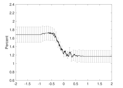
(a) Plug-In Variance Estimator

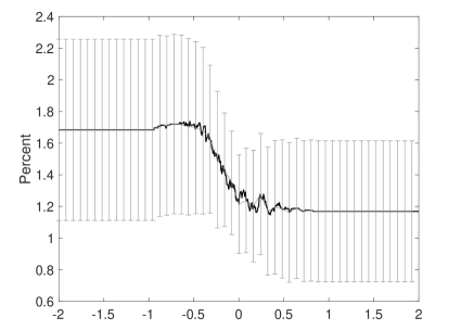
(b) Fama-MacBeth Variance Estimator

The improved precision of our new variance estimator is replicated when we shift to uniform confidence bands for the grand mean rather than pointwise confidence intervals. Figure 2 is the counterpart to Figure 1 with uniform confidence bands constructed as discussed in Section 5. The bottom chart shows the uniform confidence bands formed using the FM variance estimator. The bands are so wide as to be essentially uninformative. In contrast, the top chart displays the confidence bands formed using our new variance estimator. We can reject a constant function and also clearly reject a monotonically decreasing relationship. In contrast, we fail to reject a monontonically decreasing relationship – either linear or nonlinear.

Table 3: Pointwise Inference: This table presents the grand mean estimate, $\hat{\mu}(\beta)=T^{-1}\sum_{t=1}^{T}\hat{\mu}_{t}(\beta)$ along with pointwise upper and lower bounds for nominal coverage of 95% and 99%. Confidence intervals constructed using the plug-in variance estimator introduced in equation (5.2) are denoted by “PI-LB” abd “PI-UB” whereas those using the Fama-MacBeth variance estimator are denoted by “FM-LB” and “FM-UB”.The sample period is 1965m1–2019m12.

		90% Coverage				95% Coverage
$\beta$	$\hat{\mu}(\beta)$	PI-LB	PI-UB	FM-LB	FM-UB	PI-LB	PI-UB	FM-LB	FM-UB
-1.00	1.68	1.50	1.87	1.00	2.26	1.47	1.90	1.00	2.37
-0.50	1.72	1.57	1.87	1.06	2.27	1.54	1.90	1.06	2.38
-0.25	1.53	1.41	1.65	1.01	1.97	1.39	1.67	1.01	2.05
0.00	1.24	1.19	1.30	0.88	1.55	1.18	1.31	0.88	1.61
0.25	1.26	1.15	1.37	0.80	1.65	1.13	1.39	0.80	1.72
0.50	1.18	1.05	1.31	0.66	1.62	1.03	1.34	0.66	1.70
1.00	1.17	1.03	1.31	0.64	1.61	1.00	1.34	0.64	1.70

Figure 2: Uniform Inference on Expected Returns. This figure shows the grand mean estimate, $\hat{\mu}(\beta)=T^{-1}\sum_{t=1}^{T}\hat{\mu}_{t}(\beta)$ (black line) with associated uniform confidence bands (shaded area). The top chart constructs uniform confidence bands using the plug-in variance estimator introduced in equation (5.2) while the bottom chart uses the Fama-MacBeth variance estimator. The nominal coverage is 95%. The sample period is 1965m1–2019m12.

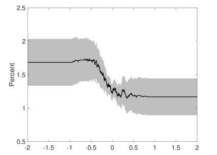
(a) Plug-In Variance Estimator

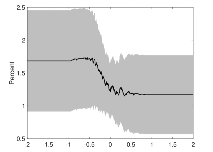
(b) Fama-MacBeth Variance Estimator

7 Conclusion

Beta-sorted portfolios are a commonly used empirical tool in asset pricing. In a first step, time-varying factor exposures are estimated by weighted regressions of asset returns on an observable risk factor to ascertain how returns co-move with the variable of interest. In a second step, individual assets are grouped into portfolios by similar factor exposures and differential returns are assessed as a function of differential exposures. Yet the simple and intuitively appealing algorithm belies a more complicated statistical setting involving a two-step estimation procedure where each stage involves non-parametric estimation.

We provide a comprehensive statistical framework which rationalizes this commonly-used estimator. Armed with this foundation we study the theoretical properties of beta-sorted portfolios linking directly to the choice of estimation window in the first step and the number of portfolios in the second step which serves as the tuning parameters for each nonparametric estimator. We introduce conditions that ensure consistency and asymptotic normality for a single cross-section and for the grand mean estimator. We also introduce new uniform inference procedures which allow for more general and varied hypothesis testing than currently available in the literature. However, we also discover some limitations of current practices and provide new guidance on appropriate implementation and interpretation of empirical results.

References

In this subsection, we show the theoretical properties of the first-step estimation of $\alpha_{it}$ and $\beta_{it}$ as in the model (2.1). For a time series $X_{t,l}$, we define $X_{t,l}=g_{l}(\xi_{t},\xi_{t-1},\cdots,\xi_{-\infty})$. $\delta_{q,m}(X_{.,l})=\max_{t}\|X_{t,l}-X_{t-m,l}^{*}\|_{q}$ with $X_{t,l}^{*}$ as a process with $\xi_{0}$ replaced by $\xi_{0}^{*}$ (i.i.d. copy of $\xi_{0}$). We define $\Theta_{m^{0},q}(f_{.})=\sum_{m\geq m^{0}}\delta_{q,m}(f_{.})$, with $m^{0}$ as an integer. Without loss of generality, we shall assume that $n\leq n_{t}\leq n_{u}$ (and without loss of generality $n_{t}$ and $n_{u}$ are of the same order) throughout the section. Define $\tilde{A}(t_{0})=\sum_{t}\mathbb{E}({X}_{t}X_{t}^{\top}|\mathcal{F}_{t-1})w(t,t_{0})$ and $\tilde{B}_{i}(t_{0})=\sum_{t}\mathbb{E}(X_{t}R_{it}|\mathcal{F}_{t-1})w(t,t_{0})$. Define ${A}(t_{0})=\sum_{t}X_{t}X_{t}^{\top}w(t,t_{0})$ and ${B}_{i}(t_{0})=\sum_{t}X_{t}R_{it}w(t,t_{0})$. Recall that $w(t,t_{0})=h^{-1}K((t-t_{0})/(Th))$. We suppress the dependency of $t_{0}$ by the elements as in $\tilde{A}(t_{0}),\tilde{B}_{i}(t_{0}),{A}(t_{0})$. We define $\overline{B}_{i}(t_{0})=\overline{B}_{i}(t_{0})=\sum_{t}\mathbb{E}(X_{t}X_{t}^{\top}|\mathcal{F}_{t-1})w(t,t_{0})b_{it_{0}}=\tilde{A}b_{it_{0}}$. We define $r_{T}=(Th)^{-1}(T^{1/q}+(Th\log T)^{1/2})$, for an integer $q>4$.

Assumption 1.

We assume that the bounded differentiable one-sided kernel function $K(.)$ takes support in [-1,0], and satisfies $\int^{0}_{-1}K(u)du=1$. $K(.)\in C^{2}[-1,0]$. $T\to\infty,h\to 0,Th\to\infty$.

Assumption 2.

Assume that $f_{t}=\tau^{\prime}(t/T)+x_{t}$, where $x_{t}$ is a stationary process. The trend function $\tau^{\prime}(.)$ is bounded by $c_{\tau}$ and is second order differentiable. $\mathbb{E}(x_{t})=0$. We assume that $\mathbb{E}(\varepsilon_{it}|\mathcal{F}_{t-1},x_{t})=0$ and it implies that $\mathbb{E}(\varepsilon_{it}|\mathcal{F}_{t-1})=0$. We define $\mathbb{E}(\varepsilon_{it}^{2}|\mathcal{F}_{t-1},x_{t})=\sigma(\mathcal{F}_{t-1},t/T)^{2}=\sigma_{t}^{2},$ and define $\mathbb{E}x_{t}=0$. $\|\varepsilon_{it}\|_{2q}\leq c$. $\mathbb{E}(\varepsilon_{it}^{2}|\mathcal{F}_{t-1},x_{t-1})=\mathbb{E}(\varepsilon_{it}^{2}|\mathcal{F}_{t-1})$. $\sigma_{\varepsilon,0}^{2}=\mathbb{E}(\varepsilon_{t_{0}}^{2})=\mathbb{E}(\sigma_{t_{0}}^{2})>0$. The error term $\varepsilon_{it_{0}}$ has finite $q$th moment with $q>4$. $(T)^{2/q-1}n_{u}^{2/q}\ll h$.

It shall be noted that $T^{2/q-1}n_{u}^{2/q}\ll h$ favors a high moment condition for example if $q=8$, we just need $T^{-3/4}n^{1/4}\ll h$.

Assumption 3.

There exists a constant $c,C_{A,\max}$ such that $\min_{t_{0}}\lambda_{\min}(T^{-1}\mathbb{E}(\tilde{A}(t_{0})))>c^{-1}>0$, $c^{-1}<\min_{t_{0}}\lambda_{min}(T^{-1}\mathbb{E}A(t_{0}))\leq\max_{t_{0}}\lambda_{max}(T^{-1}\mathbb{E}A(t_{0}))<C_{A,\max}$ and $\min_{t_{0}}\lambda_{\min}(T^{-1}\mathbb{E}(B_{i}(t_{0})))>c^{-1}>0$. $\max_{t_{0}}\lambda_{\max}(T^{-1}\mathbb{E}(B_{i}(t_{0})))<C_{B}$ for a positive constant $C_{B}$.

Assumption 4.

We define $\sigma_{x}^{2}=\mathbb{E}(x_{t}^{2})<\infty$ and $\sigma_{x4}=\mathbb{E}(x_{t}^{4})<\infty$, and we assume that they are both bounded by a positive constant $c_{x,q}$. We define the constant $c_{x}=2\sigma_{x}^{2}\int^{0}_{-1}K(s)^{2}ds$. We denote $\Sigma_{x}=\mathbb{E}[(1,x_{t})^{\top}(1,x_{t})]$, $\tilde{\tau}(t_{0}/T)=(1,\tau^{\prime}(t_{0}/T))^{\top}$. We let $\Sigma_{A}=\Sigma_{x}+\tilde{\tau}(t_{0}/T)\tilde{\tau}(t_{0}/T)^{\top}$, $\Sigma_{B}=\sigma_{\varepsilon,0}^{2}\mathbb{E}(X_{t_{0}}X^{\top}_{t_{0}})\int_{-1}^{0}K^{2}(s)ds$. Assume that both $\Sigma_{A}$ and $\Sigma_{B}$ has eigenvalues bounded from the below and the above.

Assumption 5.

(Lipschitz condition) We assume that the $\alpha_{it}=\alpha_{i}(t/T,\mathcal{F}_{t-1})$ and $\beta_{it}=\beta_{i}(t/T,\mathcal{F}_{t-1})$ satisfying for any $t,t^{\prime}\in[Th,T-Th]$, $|\alpha_{it}-\alpha_{it^{\prime}}|\leq C_{\alpha}(\mathcal{F}_{t-1})|t-t^{\prime}|/T$ and $|\beta_{it}-\beta_{it^{\prime}}|\leq C_{\beta}(\mathcal{F}_{t-1})|t-t^{\prime}|/T$, where $C_{\alpha}(\mathcal{F}_{t-1}),C_{\beta}(\mathcal{F}_{t-1})$ are two $\mathcal{F}_{t-1}$ measurable functions. Moreover,
$\max_{t}|C_{\alpha}(\mathcal{F}_{t-1})|,\max_{t}|C_{\beta}(\mathcal{F}_{t-1})|$ are bounded by constants $C_{\alpha},C_{\beta}$. Assume $\alpha_{it},\beta_{it}$ are bounded uniformly over $i,t$ .

Assumption 6.

In particular for any positive integer $m$, we assume that $\Theta_{m,2q}(f_{t})=m^{-v}$ and $\max_{t}\|f_{t}\|_{2q}$ is bounded, for $2v>1/2-1/q$, with $q>4$, for a positive constant $v$.

Define $r_{T}=(Th)^{-1}(T^{1/q}+(Th\log T)^{1/2})$. Let $q_{n}=J_{u}\vee n_{u}\vee T$ . $h\vee r_{T}\vee\sqrt{\log(q_{n})}/{\sqrt{Th}}=\delta_{T}$.

Assumption 7.

$F_{\beta,t}(x)$ is continuously differentiable on the compact interval $B_{\delta}=[\beta_{l}-\delta_{T},\beta_{u}+\delta_{T}]$ ($\delta_{T}$ is a positive constant). $\beta_{it}$ are i.i.d. conditioning on $\mathcal{G}_{t-1}$(sigma field of time invariant factors). $\varepsilon_{it}$ are independent conditioning on all three of the filtration $\cup(\mathcal{F}_{t-1},\sigma(f_{t}))$, $\mathcal{G}_{t-1}$ and $\mathcal{F}_{t-1}$ respectively. The condition density of $\beta_{it}$ is denoted as $f_{\beta,t}(x)$. $C_{\beta,max}>\max_{t}\max_{x\in B_{\delta}}f_{\beta,t}(x)>\min_{t}\min_{x\in B_{\delta}}f_{\beta,t}(x)>c_{\beta,min}>0$, which is also first order continuous differentiable with bounded derivatives. $\mathbb{E}(\beta_{it}\Phi_{it}^{*}|\mathcal{G}_{t-1})\asymp_{p}J_{t}^{-1}$, $\min_{j_{t}}\mathbb{E}_{t-1}(\Phi_{i,j_{t},t}^{*}\varepsilon_{it}^{2})\asymp_{p}J_{t}^{-1}$ and $\tilde{q}_{j_{t}}=\int^{F_{\beta,t}^{-1}(\kappa_{j})}_{F_{\beta,t}^{-1}(\kappa_{j-1})}f_{\beta,t}d\beta\asymp_{p}J_{t}^{-1}$.

Define $a_{nT}=\max_{t}(\sqrt{\delta_{T}}c_{n_{u}T}/{\sqrt{n_{t}}})\vee\sqrt{\log T}\sqrt{n_{t}}^{-1}$, where $c_{n_{u}T}$ is a positive constant.

Assumption 8.

We let $\max_{t}n_{t}\leq n_{u}$, $n\leq n_{t}$, $J\leq J_{t}\leq J_{u}$, $J_{u}\asymp J$ and $n_{u}\asymp n$. Recall $r_{T}=(Th)^{-1}(T^{1/q}+(Th\log T)^{1/2})$, with $q>4$. We assume that Assumptions 16 to 21 are maintained such that $\max_{i}\sup_{t}|\widehat{\beta}_{it}-\beta_{it}|\lesssim_{\mathbb{P}}\delta_{T}$ and $J_{u}^{-1}\gg\frac{\sqrt{\log(q_{n})}}{\sqrt{n}}$ . $\delta_{T}\to 0$ , $r_{T}\to 0$. We assume that $a_{nT}\to 0$.

We note that the above assumption implies that $J\log q_{n}/{n}\ll 1$. Define $\delta=(\delta_{T}+a_{nT})^{1/2}\sqrt{\log q_{n}}/{\sqrt{n}}$.

Assumption 9.

$J(\delta_{T}+a_{nT})^{1/2}\sqrt{\log q_{n}}/{\sqrt{n}}\ll 1$.

Assumption 10.

We assume that ${\alpha}(\beta)$ is continuously differentiable of the first order, and with the first derivative bounded from the above by positive constant $c_{\alpha}$.

We first order observations as $\ell=\ell(i,t)=\sum_{t_{0}=1}^{t-1}n_{t}+i$, $1\leq i\leq n_{t},1\leq t_{0}\leq T$. We let $\mathcal{F}^{\beta}_{\ell-1}$ denote the sigma field of $\beta_{\ell}$ up to the order of $\ell-1$.

Assumption 11.

We let $\tilde{\beta}_{\ell,j}=\beta_{\ell,j}-F^{-1}_{\beta,t}(\kappa_{j})$. $\tilde{\beta}_{\ell,j}$ are different over time, however the dependence can still decay as the series of $\beta_{it}$. We assume that $\bm{1}(-u\leq\tilde{\beta}_{\ell,j}<u)=\psi_{\ell,j}(u)$. We assume that $\max_{\ell,j}\mathbb{E}(\beta_{\ell,j}^{2}\bm{1}(-u\leq\tilde{\beta}_{\ell,j}<u)|\mathcal{F}^{\beta}_{\ell-1})\leq C\beta_{u}^{2}u$, $\max_{\ell,j}\mathbb{E}(\varepsilon_{\ell}^{2}\bm{1}(-u\leq\tilde{\beta}_{\ell,j}<u)|\mathcal{F}^{\beta}_{\ell-1})\leq C\beta_{u}^{2}u$, for a constant $C$. Moreover we assume that $\|\max_{j}\mathbb{E}(\psi_{.,j}(u)|\mathcal{F}^{\beta}_{.-1})\|_{q,\zeta}\leq u^{1/q}C_{q,\zeta}$, $\|\max_{j}\mathbb{E}(\psi_{.,j}(u)\beta_{.,j}|\mathcal{F}^{\beta}_{.-1})\|_{q,\zeta}\leq u^{1/q}C^{\prime}_{q,\zeta}$, for an integer $q>4$.

Define ${\overline{\delta}}_{T}=\sqrt{\log q_{n}}/\sqrt{nT}\vee h\vee\sqrt{\log(q_{n})}/{\sqrt{nTh}}$.

Assumption 12.

${(a_{nT}/{\sqrt{T}}+\overline{\delta}_{T})}\vee J{(a_{nT}+{\delta}_{T})}^{1/2}/{\sqrt{nT}}\lesssim h\vee J^{-1}\ll\sqrt{T}^{-1}$.

We shall give an example on the plausible rate of $n,T,J,h$ which is admissible to the above assumptions. For example, we can assume that $n=T$, $J=\textit{O}(T^{1/3})$ and $h=\textit{O}(T^{-1/3})$.

We notice that the conditions $\|\max_{j}\mathbb{E}(\psi_{.,j}(u)\beta_{.}|\mathcal{F}^{\beta}_{.-1})\|_{q,\zeta}\leq u^{1/q}C^{\prime}_{q,\zeta}$ are easily satisfied. Let us illustrate for the stationary case of $\beta_{\ell}$. For example if we assume that $f_{\beta,t}(\beta|\mathcal{F}^{\beta}_{t-1})$ is differentiable with respect to $\beta$ and its i.i.d. innovation $\varepsilon_{0}$ (slightly abuse of notation), then we can derive that,

$$\mathbb{E}(\psi_{.,j}(u)\beta_{\ell,j}|\mathcal{F}^{\beta}_{\ell-1})-\mathbb{E}(\psi_{.,j}(u)\beta_{\ell,j}|\mathcal{F}^{\beta*}_{\ell-1})$$

$$= \int^{u+F^{-1}_{\beta,t}(\kappa_{j})}_{-u+F^{-1}_{\beta,t}(\kappa_{j})}\beta f_{\beta,t}(\beta|\mathcal{F}^{\beta}_{\ell-1})d\beta-\int^{{u+F^{-1}_{\beta,t}(\kappa_{j})}}_{-u+F^{-1}_{\beta,t}(\kappa_{j})}\beta f_{\beta,t}(\beta|\mathcal{F}^{{\beta}*}_{\ell-1})d\beta$$

$$\leq 2u|\varepsilon_{0}-\varepsilon_{0}^{*}||\beta_{u}\partial f(\tilde{\beta}|\tilde{\mathcal{F}}_{\ell-1})/(\partial\varepsilon_{0}\partial\beta)|,$$

where $\tilde{\beta}$ is a point between the intersection of $\cap_{j}(-u+F_{\beta,t}^{-1}(\kappa_{j}),u+F_{\beta,t}^{-1}(\kappa_{j}))$, and $\tilde{\mathcal{F}}_{\ell-1}$ is the filtration with $\varepsilon_{0}$ replaced by some value. We take the $\|.\|_{q}$ norm of the above object. If we can ensure that $|\varepsilon_{0}-\varepsilon_{0}^{*}||\beta_{u}||\partial f(\tilde{\beta}|\tilde{\mathcal{F}}_{\ell-1})/(\partial\varepsilon_{0}\partial\beta)\|_{q}$ decrease sufficient fast according to the lag $\ell$, then the conditions holds. We let $\delta^{\prime}=\Delta_{T}/{\sqrt{T}}$. Define $\mathbb{N}_{J}=\bigcup_{t=1\cdots,T}N_{J_{t}}$. ${\overline{\delta}}_{T}=\sqrt{\log q_{n}}/\sqrt{nT}\vee h\vee\sqrt{\log(q_{n})}/{\sqrt{nTh}}$.

Assumption 13.

Let $\widehat{\sigma}^{1/2}_{D}(\beta_{1,2,3})$ be a consistent estimator for $\sigma_{D}(\beta_{1,2,3})$ satisfying $\widehat{\sigma}_{D}(\beta_{1,2,3})^{1/2}-{\sigma}_{D}(\beta_{1,2,3})^{1/2}=\textit{o}{{}_{\mathbb{P}}}(r_{1,2,3})$, and the rate $r_{1,2,3}\to 0$. $\sigma_{d}(\beta)$ is bounded from the below and the above uniformly over $\beta$. $\max_{j,t}\|\Phi_{i,j,t}^{*}\varepsilon_{it}\tilde{q}_{j}^{-1}\|_{q}\lesssim J^{1-1/q}$.

Since we have $1/{J_{t}}*{J_{t}}^{2}({J_{t}}^{-1}(\delta_{T}+a_{nT})+\sqrt{\delta_{T}}T^{1/2q}(n_{t}^{-1/2}J_{t}^{-1/2}))=\textit{o}{{}_{\mathbb{P}}}(\text{$\text{$\text{$\delta_{2}$}$}$})$ and $(1/J_{t}(l_{n,T}/n_{t}+J_{t}^{-1})J_{t}^{2}(l_{n,T}/n_{t})J_{t}^{-1}J_{t}^{2})=\textit{o}{{}_{\mathbb{P}}}(\delta_{1}).$ Recall that $\delta_{1}=\sqrt{a_{nT}+\delta_{T}}J_{t}/\sqrt{n_{t}}+a_{nT}+\delta_{T}$, $\delta_{2}=\delta_{T}+a_{nT}+\sqrt{\delta_{T}}T^{1/(2q)}n_{t}^{-1/2}J_{t}^{1/2}$.

Assumption 14.

Let $\varepsilon_{it}=_{d}\sigma_{t}\eta_{it}$ conditional on $\mathcal{F}_{t-1}$, with $\sigma_{t}^{2}=\mathbb{E}(\varepsilon_{it}^{2}|\mathcal{F}_{t-1})$, and $\eta_{it}$ be a standard Gaussian random variable defined on a proper probability space. Exists two positive constants $c,C>0$,

$$c\leq\min_{j}\sigma_{j}\leq\max_{j}\sigma_{j}\leq C.$$

And we have $\delta_{1T}+\delta_{2T}<<1/{\sqrt{\log J}}.$ $n_{t}^{-1/2+1/(2q)}\sqrt{J_{t}}<<\sqrt{J_{t}}^{-1}.$ Moreover, $\sqrt{n_{t}/J_{t}}(h\vee J_{t}^{-1})\to 0$.

Assumption 15.

Assume that with probability one, $E_{n_{t},j}/\sigma_{j}$s are bounded from the below and the above for all $t,j$. $\sup_{\beta}\{\widehat{\sigma}(\beta)^{1/2}-\sigma(\beta)^{1/2}\}=\textit{O}_{\mathbb{P}}(r_{\sigma})$ for some constant $r_{\sigma}$. Assume $r_{\sigma}T^{-1/2+1/2q}J_{a}^{1/2q}\to 0$ and $r_{\sigma}\to 0$. $c\leq\inf_{\beta}\sigma(\beta)=\sup_{\beta}\sigma(\beta)\leq C$. $c\leq\min_{\beta}\tilde{\sigma}(\beta)=\sup_{\beta}\tilde{\sigma}(\beta)\leq C$. $\|E_{n_{t},j}-E_{n_{t},j-1}\|_{2q}\leq cJ_{t}^{-1}$, for a positive constant $c>0$. $\|f_{t}-\mathbb{E}(f_{t}|\mathcal{F}_{t-1})\|_{2q}<C,$ for a positive $C>0$. Assume that the grid is $\overline{\beta}_{v}=[\beta_{1},\beta_{2},\cdots,\beta_{c/\tilde{\delta}}]$. This corresponds to ${J}_{a,\delta}$ distinct value of $\beta$. We shall assume that for avoiding singularity of the variance covariance matrix. We need to ensure that $\sigma(\beta_{j},\beta_{j^{\prime}})\neq\sigma(\beta_{j},\beta_{j})\quad\mbox{or}\quad\sigma(\beta_{j^{\prime}},\beta_{j^{\prime}})$. Let $[\widehat{\sigma}(\beta_{i},\beta_{i^{\prime}})/{\widehat{\sigma}^{1/2}(\beta_{i})\widehat{\sigma}(\beta_{i^{\prime}})^{1/2}}]_{i,i^{\prime}}=\Sigma_{J_{a,\delta},J_{a,\delta}}$. We shall assume that $c<\lambda_{\min}(\Sigma_{J_{a},\delta})<\lambda_{\max}(\Sigma_{J_{a},\delta})<C^{\prime}$, with $C^{\prime},c>0$. Let $J_{a,\delta}\lesssim\exp(T^{\varepsilon^{\prime}})$, with $\varepsilon^{\prime}=1/9$.

Appendix A Setup

A.1 Assumptions

In this subsection, we show the theoretical properties of the first-step estimation of $\alpha_{it}$ and $\beta_{it}$. For a time series $X_{t,l}$, we define $X_{t,l}=g_{l}(\xi_{t},\xi_{t-1},\cdots,\xi_{-\infty})$. $\delta_{q,m}(X_{.,l})=\max_{t}\|X_{t,l}-X_{t-m,l}^{*}\|_{q}$ with $X_{t,l}^{*}$ as a process with $\xi_{0}$ replaced by $\xi_{0}^{*}$ (i.i.d. copy of $\xi_{0}$). We define $\Theta_{m^{0},q}(f_{.})=\sum_{m\geq m^{0}}^{\infty}\delta_{q,m}(f_{.})$, with $m^{0}$ as an integer. Without loss of generality, we shall assume that $n\leq n_{t}\leq n_{u}$ (and without loss of generality $n_{t}$ and $n_{u}$ are of the same order) throughout the section. Define $\tilde{A}(t_{0})=\sum_{t=1}^{T}\mathbb{E}({X}_{t}X_{t}^{\top}|\mathcal{F}_{t-1})w(t,t_{0})$ and $\tilde{B}_{i}(t_{0})=\sum_{t=1}^{T}\mathbb{E}(X_{t}R_{it}|\mathcal{F}_{t-1})w(t,t_{0})$. Define ${A}(t_{0})=\sum_{t=1}^{T}X_{t}X_{t}^{\top}w(t,t_{0})$ and ${B}_{i}(t_{0})=\sum_{t=1}^{T}X_{t}R_{it}w(t,t_{0})$. Recall that $w(t,t_{0})=h^{-1}K((t-t_{0})/(Th))$. We suppress the dependency of $t_{0}$ by the elements as in $\tilde{A}(t_{0}),\tilde{B}_{i}(t_{0}),{A}(t_{0})$. We define
$\overline{B}_{i}(t_{0})=\overline{B}_{i}(t_{0})=\sum_{t=1}^{T}\mathbb{E}(X_{t}X_{t}^{\top}|\mathcal{F}_{t-1})w(t,t_{0})b_{it_{0}}=\tilde{A}b_{it_{0}}$. We define $r_{T}=(Th)^{-1}(T^{1/q}+(Th\log T)^{1/2})$, for an integer $q>4$.

Assumption 16.

We assume that the bounded differentiable one-sided kernel function $K(.)$ takes support in [-1,0], and satisfies $\int^{0}_{-1}K(u)du=1$. $K(.)\in C^{2}[-1,0]$. $T\to\infty,h\to 0,Th\to\infty$.

Assumption 17.

Assume that $f_{t}=\tau^{\prime}(t/T)+x_{t}$, where $x_{t}$ is a stationary process. The trend function $\tau^{\prime}(.)$ is bounded by $c_{\tau}$ and is second order differentiable. $\mathbb{E}(x_{t})=0$. We assume that $\mathbb{E}(\varepsilon_{it}|\mathcal{F}_{t-1},x_{t})=0$ and it implies that $\mathbb{E}(\varepsilon_{it}|\mathcal{F}_{t-1})=0$. We define $\mathbb{E}(\varepsilon_{it}^{2}|\mathcal{F}_{t-1},x_{t})=\sigma(\mathcal{F}_{t-1},t/T)^{2}=\sigma_{t}^{2}$. $\|\varepsilon_{it}\|_{2q}\leq c$, and $c>0$. $\mathbb{E}(\varepsilon_{it}^{2}|\mathcal{F}_{t-1},x_{t-1})=\mathbb{E}(\varepsilon_{it}^{2}|\mathcal{F}_{t-1})$. $\sigma_{\varepsilon,0}^{2}=\mathbb{E}(\varepsilon_{t_{0}}^{2})=\mathbb{E}(\sigma_{t_{0}}^{2})>0$. The error term $\varepsilon_{it_{0}}$ has finite $q$th moment with $q>4$. $(T)^{2/q-1}n_{u}^{2/q}\ll h$.

It shall be noted that $T^{2/q-1}n_{u}^{2/q}\ll h$ favors a high moment condition for example if $q=8$, we just need $T^{-3/4}n^{1/4}\ll h$.

Assumption 18.

There exists a constant $c,C_{A,\max}$ such that $\min_{t_{0}}\lambda_{\min}(T^{-1}\mathbb{E}(\tilde{A}(t_{0})))>c^{-1}>0$, $c^{-1}<\min_{t_{0}}\lambda_{min}(T^{-1}\mathbb{E}[A(t_{0})])\leq\max_{t_{0}}\lambda_{max}(T^{-1}\mathbb{E}[A(t_{0})])<C_{A,\max}$ and $\min_{t_{0}}\lambda_{\min}(T^{-1}\mathbb{E}(B_{i}(t_{0})))>c^{-1}>0$. $\max_{t_{0}}\lambda_{\max}(T^{-1}\mathbb{E}(B_{i}(t_{0})))<C_{B}$ for a positive constant $C_{B}$.

Assumption 19.

We define $\sigma_{x}^{2}=\mathbb{E}(x_{t}^{2})<\infty$ and $\sigma_{x4}=\mathbb{E}(x_{t}^{4})<\infty$, and we assume that they are both bounded by a positive constant $c_{x,q}$. We define the constant $c_{x}=2\sigma_{x}^{2}\int^{0}_{-1}K(s)^{2}ds$. We denote $\Sigma_{x}=\mathbb{E}[(1,x_{t})^{\top}(1,x_{t})]$, $\tilde{\tau}(t_{0}/T)=(1,\tau^{\prime}(t_{0}/T))^{\top}$. We let $\Sigma_{A}=\Sigma_{x}+\tilde{\tau}(t_{0}/T)\tilde{\tau}(t_{0}/T)^{\top}$, $\Sigma_{B}=\sigma_{\varepsilon,0}^{2}\mathbb{E}(X_{t_{0}}X^{\top}_{t_{0}})\int_{-1}^{0}K^{2}(s)ds$. Assume that both $\Sigma_{A}$ and $\Sigma_{B}$ has eigenvalues bounded from the below and the above.

Assumption 20.

(Lipschitz condition) We assume that the $\alpha_{it}=\alpha_{i}(t/T,\mathcal{F}_{t-1})$ and $\beta_{it}=\beta_{i}(t/T,\mathcal{F}_{t-1})$ satisfying for any $t,t^{\prime}\in[Th,T-Th]$, $|\alpha_{it}-\alpha_{it^{\prime}}|\leq C_{\alpha}(\mathcal{F}_{t-1})|t-t^{\prime}|/T$ and $|\beta_{it}-\beta_{it^{\prime}}|\leq C_{\beta}(\mathcal{F}_{t-1})|t-t^{\prime}|/T$, where $C_{\alpha}(\mathcal{F}_{t-1}),C_{\beta}(\mathcal{F}_{t-1})$ are two $\mathcal{F}_{t-1}$ positive measurable functions. Moreover,
$\max_{t}|C_{\alpha}(\mathcal{F}_{t-1})|,\max_{t}|C_{\beta}(\mathcal{F}_{t-1})|$ are bounded by constants $C_{\alpha},C_{\beta}$. Assume $\alpha_{it},\beta_{it}$ are bounded uniformly over $i,t$ .

Remark A.1.

Note that under our assumptions we have that

$$\mathbb{E}T^{-1}\sum_{t=1}^{T}x_{t}^{2}w(t,t_{0})=\sigma_{x}^{2}T^{-1}\sum_{t=1}^{T}w(t,t_{0})=\sigma^{2}_{x}.$$ (A.1)

And

$$T^{-1}\sum_{t=1}^{T}\tau^{\prime}(t/T)^{2}w(t,t_{0})=\tau^{\prime}(t_{0}/T)^{2}+\textit{O}(h).$$ (A.2)

$$\mathop{\hbox{Var}}(\sqrt{h/T}^{-1}\sum_{t=1}^{T}w(t,t_{0})\varepsilon_{it}f_{t})=\sigma_{\varepsilon,0}^{2}(\sigma^{2}_{x}+\tau^{\prime}(t_{0}/T)^{2})\int^{0}_{-1}K(s)^{2}ds+\textit{O}(h).$$ (A.3)

Thus we conclude $T^{-1}\mathbb{E}(A)=\Sigma_{x}+\tilde{\tau}(t_{0}/T)\tilde{\tau}(t_{0}/T)^{\top}+\textit{O}(h)$.

Remark A.2 (Admissible processes of $\beta$).

Suppose that $\beta_{it}=G_{\beta}(\eta_{i},g_{1},\cdots,g_{t-1},f_{1},\cdots,f_{t-1},\omega_{it-1})$, where $\eta_{i}$ is iid over $i$, $g_{t}$ is i.i.d. factors over $t$, and $\omega_{it-1}$ are i.i.d. over $t$ and $i$. We denote the common factor sigma field as $\mathcal{G}_{t-1}=\sigma(f_{1},\cdots,f_{t-1},g_{1},\cdots,g_{t-1})$. The function $\beta_{it}$ shall be smooth over time, and conditional i.i.d. conditioning on the sigma field $\mathcal{G}_{t-1}$.

Assumption 21.

In particular for any positive integer $m$, we assume that $\Theta_{m,2q}(f_{t})=m^{-v}$ and $\max_{t}\|f_{t}\|_{2q}$ is bounded, for $2v>1/2-1/q$, with $q>4$, for a positive constant $v$.

Remark A.3.

We shall see that Assumption 16 ensures the basic property of the kernel functions. The one-sided kernel is adopted to avoid the look- ahead bias term. Also it is important for us to adopt the one-sided kernel in this step, as in the second step, our theoretical results works with conditioning on the filtration in the past. The generated error induced by estimating beta is thus fixed with respect to the conditioned filtration. Assumption 17 poses some general structure of the factor $f_{t}$ and also impose some basic assumptions of the error term $\varepsilon_{it}$ to ensure the validity of our estimator. We set the factor to be a trend stationary process, and we assume homoscedasticity over time for the simplicity of our analysis. It would be not hard to extend to more general settings. Moreover, we also assume finite $2q$ th moment. Assumption 18 sets the proper behavior of the matrix in the population. It is related to the identification of our estimator. Assumptions 19- 21 are regular conditions on the decay rate of the dependency for factors. Note that we can relax the assumption on the boundedness of ${\alpha}_{it}$ and $\beta_{it}$. Assumption 21 implies that $\Theta_{m,q}(\mathbb{E}(f_{.}|f_{.-1}))$, $\Theta_{m,q}(\mathbb{E}(f_{.}|f_{.-1}))$ are bounded by constants $c_{\theta}$, $\Theta_{m,q}(f^{2}_{.})=m^{-v}$, for a positive constant $v$. In sum, we shall assume that the alphas and betas are suffiiciently smooth over time, and the temporal dependency of factors shall be weak.

Define $r_{T}=(Th)^{-1}(T^{1/q}+(Th\log T)^{1/2})$. Let $q_{n}=J_{u}\vee n_{u}\vee T$ . $h\vee r_{T}\vee\sqrt{\log(q_{n})}/{\sqrt{Th}}=\delta_{T}$.

Assumption 22.

$F_{\beta,t}(x)$ is continuously differentiable on the compact interval $B_{\delta}=[\beta_{l}-\delta_{T},\beta_{u}+\delta_{T}]$ ($\delta_{T}$ is a positive constant). $\beta_{it}$ are i.i.d. conditioning on $\mathcal{G}_{t-1}$(sigma field of time invariant factors). $\varepsilon_{it}$ are independent conditioning on all three of the filtration $\cup(\mathcal{F}_{t-1},\sigma(f_{t}))$, $\mathcal{G}_{t-1}$ or $\mathcal{F}_{t-1}$ respectively. The condition density of $\beta_{it}$ is denoted as $f_{\beta,t}(x)$. $C_{\beta,max}>\max_{t}\max_{x\in B_{\delta}}f_{\beta,t}(x)>\min_{t}\min_{x\in B_{\delta}}f_{\beta,t}(x)>c_{\beta,min}>0$, which is also first order continuous differentiable with bounded derivatives. $\mathbb{E}(\beta_{it}\Phi_{it}^{*}|\mathcal{G}_{t-1})\asymp_{p}J_{t}^{-1}$, $\min_{j_{t}}\mathbb{E}_{t-1}(\Phi_{i,j_{t},t}^{*}\varepsilon_{it}^{2})\asymp_{p}J_{t}^{-1}$ and $\tilde{q}_{j_{t}}=\int^{F_{\beta,t}^{-1}(\kappa_{j})}_{F_{\beta,t}^{-1}(\kappa_{j-1})}f_{\beta,t}d\beta\asymp_{p}J_{t}^{-1}$.

Remark A.4 (Discussion of the conditional iid assumptions for $\beta_{it}$.).

Suppose $Z_{it}$ and $Z_{t}$ are observable. Let us look the simplest model

$$R_{it}=\alpha_{it}+\beta_{it}f_{t}+\varepsilon_{it},$$ (A.4)

where $\alpha_{it}$ is a function of $\beta_{it}$. We see that $Z_{t}$ and $Z_{t-1}(U_{it})$ are measurable with respect to $\mathcal{F}_{t-1}$. Suppose that $U_{it}$ are iid random variables over time (independent of any object as the above). In Gagliardini, Ossola, and Scaillet (2019), they assume,

$$\beta_{it}(U_{it})=B(U_{it})Z_{t-1}+C(U_{it})Z_{t-1}(U_{it}),$$ (A.5)

where $B(U_{it}),C(U_{it})$ are parameters which are solely functions of $U_{it}$.

We can observe that conditioning on ${\mathcal{G}}_{t-1}=\sigma(Z_{t-1}(.),Z_{t-1})$, $\beta_{it}(U_{it})$ will have only source of randomness from $(U_{it})_{i,t}$ and therefore are iid over $i$. We can express $\beta_{it}(U_{it})=g(U_{it},Z_{t-1},Z_{t-1}(.))$. To ensure that $g(U_{it},Z_{t-1},Z_{t-1}(.))$ is smooth over $t$. Furthermore the smoothness assumption on $Z_{t-1}$ and $Z_{t-1}(U_{it})$ over $t$ is required for us and but NOT for required for Gagliardini, Ossola, and Scaillet (2019). However, the structure in Equation (A.5) is not necessary for us, therefore there exist models where we can cover but not covered by Gagliardini, Ossola, and Scaillet (2019). For example if we set, $\beta_{t}$ is a vector of $\beta_{it}$. $n_{t}=n$,

$$\beta_{t}=c\eta_{t-2}+a(t/T)\eta_{t-1},$$ (A.6)

where $\eta_{t}$ are iid random vectors over $t$, and forms random smooth curve over $t$. $a(t/T)$ is a smooth trend function over time, such as $a(t/T)=(t/T)^{2}$. $\eta_{t-1},\eta_{t-2}$ are measurable to $\mathcal{F}_{t-1}$. The structure in Gagliardini, Ossola, and Scaillet (2019) is then violated.

Define $a_{nT}=\max_{t}(\sqrt{\delta_{T}}c_{n_{u}T}/{\sqrt{n_{t}}})\vee\sqrt{\log T}\sqrt{n_{t}}^{-1}$, where $c_{n_{u}T}$ is a positive constant.

Assumption 23.

We let $\max_{t}n_{t}\leq n_{u}$, $n\leq n_{t}$, $J\leq J_{t}\leq J_{u}$, $J_{u}\asymp J$ and $n_{u}\asymp n$. Recall $r_{T}=(Th)^{-1}(T^{1/q}+(Th\log T)^{1/2})$, with $q>4$. We assume that Assumptions 16 to 21 are maintained such that $\max_{i}\sup_{t}|\widehat{\beta}_{it}-\beta_{it}|\lesssim_{\mathbb{P}}\delta_{T}$ and $J_{u}^{-1}\gg\frac{\sqrt{\log(q_{n})}}{\sqrt{n}}$ . $\delta_{T}\to 0$ , $r_{T}\to 0$. We assume that $a_{nT}\to 0$. We note that the above assumption implies that $J\log q_{n}/{n}\ll 1$. Define $\delta=(\delta_{T}+a_{nT})^{1/2}\sqrt{\log q_{n}}/{\sqrt{n}}$. $J(\delta_{T}+a_{nT})^{1/2}\sqrt{\log q_{n}}/{\sqrt{n}}\ll 1$.

Assumption 24.

We assume that ${\alpha}(\beta)$ is continuously differentiable of the first order, and with the first derivative bounded from the above by a positive constant $c_{\alpha}$.

Remark A.5.

Asssumption 22 is regarding the property of the density of $\beta_{it}$. Assumption 23 sets the property of the uniform rate of $\beta_{it}$. We see that it corresponds to Theorem B.6. Assumption 23 assumes the relative rate of $n_{t}$ and $J_{t}$ . Assumption 24 assumes the smoothness of the function $\alpha(.)$.

Remark A.6.

(Discussion of rate) We assume that $q$ to be sufficiently large and the choice of $h$ and $n_{u}$ are satisfied so that

$$\sqrt{\log(n_{u}T)}\gg T^{1/q}(Th)^{-1/2},$$

then $\delta_{T}=h+\sqrt{\log(n_{u}T)}/\sqrt{Th}$. Assume that

$$\sqrt{\log(n_{u}T)}/{\sqrt{n}}\ll 1,$$

then $a_{nT}=\sqrt{h/n}+\sqrt{\log T}/\sqrt{n}$. Thus $\delta_{T}+a_{nT}=\sqrt{\log T}/\sqrt{n}\vee h\vee\sqrt{\log(n_{u}T)}/{\sqrt{Th}}$. Assumption 24 thus assumes that

$$(\sqrt{\log T}/\sqrt{n}\vee h\vee\sqrt{\log(n_{u}T)}/{\sqrt{Th}})^{1/2}J/{\sqrt{n_{t}}}\ll 1.$$

We first order observations as $\ell=\ell(i,t)=\sum_{t_{0}=1}^{t-1}n_{t}+i$, $1\leq i\leq n_{t},1\leq t_{0}\leq T$. We let $\mathcal{F}^{\beta}_{\ell-1}$ denote the sigma field of $\beta_{\ell}$ up to the order of $\ell-1$.

Assumption 25.

We let $\tilde{\beta}_{\ell,j}=\beta_{\ell,j}-F^{-1}_{\beta,t}(\kappa_{j})$. $\tilde{\beta}_{\ell,j}$ are different over time, however the dependence can still decay as the series of $\beta_{it}$. We assume that $\bm{1}(-u\leq\tilde{\beta}_{\ell,j}<u)=\psi_{\ell,j}(u)$. We assume that $\max_{\ell,j}\mathbb{E}(\beta_{\ell,j}^{2}\bm{1}(-u\leq\tilde{\beta}_{\ell,j}<u)|\mathcal{F}^{\beta}_{\ell-1})\leq C\beta_{u}^{2}u$, $\max_{\ell,j}\mathbb{E}(\varepsilon_{\ell}^{2}\bm{1}(-u\leq\tilde{\beta}_{\ell,j}<u)|\mathcal{F}^{\beta}_{\ell-1})\leq C\beta_{u}^{2}u$, for a constant $C$. Moreover we assume that $\|\max_{j}\mathbb{E}(\psi_{.,j}(u)|\mathcal{F}^{\beta}_{.-1})\|_{q,\zeta}\leq u^{1/q}C_{q,\zeta}$, $\|\max_{j}\mathbb{E}(\psi_{.,j}(u)\beta_{.,j}|\mathcal{F}^{\beta}_{.-1})\|_{q,\zeta}\leq u^{1/q}C^{\prime}_{q,\zeta}$, for an integer $q>4$.

Define ${\overline{\delta}}_{T}=\sqrt{\log q_{n}}/\sqrt{nT}\vee h\vee\sqrt{\log(q_{n})}/{\sqrt{nTh}}$.

Assumption 26.

${(a_{nT}/{\sqrt{T}}+\overline{\delta}_{T})}\vee J{(a_{nT}+{\delta}_{T})}^{1/2}/{\sqrt{nT}}\lesssim h\vee J^{-1}\ll\sqrt{T}^{-1}$.

Remark A.7.

Following the rate discussion of Remark A.6, the above conditions can be implied by

$$\sqrt{\log q_{n}}/(\sqrt{nT})\ll h^{3/2}\vee h^{1/2}J^{-1},$$

$$\{{(\log q_{n})^{1/4}}/{n^{1/4}}\vee h^{1/2}\vee(\sqrt{\log q_{n}}/{\sqrt{Th}})^{1/2}\}\lesssim\sqrt{nT}(J^{-1}h\vee J^{-2})\ll\sqrt{n}.$$

We shall give an example on the plausible rate of $n,T,J,h$ which is admissible to the above assumptions. For example, we can assume that $n=T$, $J=\textit{O}(T^{1/3})$ and $h=\textit{O}(T^{-1/3})$.

For a positive constant $C^{\prime}_{q,\zeta}$, we notice that the conditions $\|\max_{j}\mathbb{E}(\psi_{.,j}(u)\beta_{.}|\mathcal{F}^{\beta}_{.-1})\|_{q,\zeta}\leq u^{1/q}C^{\prime}_{q,\zeta}$ are easily satisfied. Let us illustrate for the stationary case of $\beta_{\ell}$. Let $f_{\beta,t}(\beta|.),F_{\beta,t}(\beta|.)$ be density and distribution function corresponding to different filtrations. For example if we assume that $f_{\beta,t}(\beta|\mathcal{F}^{\beta}_{t-1})$ is differentiable with respect to $\beta$ and its i.i.d. innovation $\varepsilon_{0}$ (slightly abuse of notation), then we can derive that,

$$\mathbb{E}(\psi_{.,j}(u)\beta_{\ell,j}|\mathcal{F}^{\beta}_{\ell-1})-\mathbb{E}(\psi_{.,j}(u)\beta_{\ell,j}|\mathcal{F}^{\beta*}_{\ell-1})$$

$$= \int^{u+F^{-1}_{\beta,t}(\kappa_{j})}_{-u+F^{-1}_{\beta,t}(\kappa_{j})}\beta f_{\beta,t}(\beta|\mathcal{F}^{\beta}_{\ell-1})d\beta-\int^{{u+F^{-1}_{\beta,t}(\kappa_{j})}}_{-u+F^{-1}_{\beta,t}(\kappa_{j})}\beta f_{\beta,t}(\beta|\mathcal{F}^{{\beta}*}_{\ell-1})d\beta$$

$$\leq 2u|\varepsilon_{0}-\varepsilon_{0}^{*}||\beta_{u}\partial f(\tilde{\beta}|\tilde{\mathcal{F}}_{\ell-1})/(\partial\varepsilon_{0}\partial\beta)|,$$

where $\tilde{\beta}$ is a point between the intersection of $\cap_{j}(-u+F_{\beta,t}^{-1}(\kappa_{j}),u+F_{\beta,t}^{-1}(\kappa_{j}))$, and $\tilde{\mathcal{F}}_{\ell-1}$ is the filtration with $\varepsilon_{0}$ replaced by some value. We take the $\|.\|_{q}$ norm of the above object. If we can ensure that $|\varepsilon_{0}-\varepsilon_{0}^{*}||\beta_{u}||\partial f(\tilde{\beta}|\tilde{\mathcal{F}}_{\ell-1})/(\partial\varepsilon_{0}\partial\beta)\|_{q}$ decrease sufficient fast according to the lag $\ell$, then the conditions holds. We let $\delta^{\prime}=\Delta_{T}/{\sqrt{T}}$. Define $\mathbb{N}_{J}=\bigcup_{t=1\cdots,T}N_{J_{t}}$. ${\overline{\delta}}_{T}=\sqrt{\log q_{n}}/\sqrt{nT}\vee h\vee\sqrt{\log(q_{n})}/{\sqrt{nTh}}$.

Remark A.8.

Following the rate discussion of Remark A.6, the above conditions can be implied by

$$\sqrt{\log q_{n}}/(\sqrt{nT})\ll h^{3/2}\vee h^{1/2}J^{-1},$$

$$\{{(\log q_{n})^{1/4}}/{n^{1/4}}\vee h^{1/2}\vee(\sqrt{\log q_{n}}/{\sqrt{Th}})^{1/2}\}\lesssim\sqrt{nT}(J^{-1}h\vee J^{-2})\ll\sqrt{n}.$$

Assumption 27.

Let $\widehat{\sigma}^{1/2}_{D}(\beta_{1,2,3})$ be a consistent estimator for $\sigma_{D}(\beta_{1,2,3})$ satisfying $\widehat{\sigma}_{D}(\beta_{1,2,3})^{1/2}-{\sigma}_{D}(\beta_{1,2,3})^{1/2}=\textit{o}{{}_{\mathbb{P}}}(r_{1,2,3})$, and the rate $r_{1,2,3}\to 0$. $\sigma_{d}(\beta)$ is bounded from the below and the above uniformly over $\beta$. $\max_{j,t}\|\Phi_{i,j,t}^{*}\varepsilon_{it}\tilde{q}_{j}^{-1}\|_{q}\lesssim J^{1-1/q}$.

Remark A.9.

(Inconsistency of $\widehat{\mu}_{t}(\beta)$ for fixed $t$.) To facilitate the inference for fix $t$ we shall consider the following procedure. Since by Theorem B.6,

$$|\widehat{a}_{t}-a_{t}^{*}-\operatorname*{diag}(\tilde{q}_{jt})^{-1}n_{t}^{-1}\Phi_{t}^{*}\tilde{\varepsilon}_{t}|_{\infty}=\textit{o}{{}_{\mathbb{P}}}(1).$$ (A.7)

We see that

$$[n_{t}^{-1}\Phi_{t}^{*}\tilde{\varepsilon}_{t}]_{j}=n_{t}^{-1}\sum_{i=1}^{n_{t}}\Phi_{i,j,t}^{*}\tilde{\varepsilon}_{it},$$

$$= n_{t}^{-1}\sum_{i=1}^{n_{t}}\Phi_{i,j,t}^{*}\beta_{it}(f_{t}-\mathbb{E}(f_{t}|\mathcal{F}_{t-1}))+n_{t}^{-1}\sum_{i=1}^{n_{t}}\Phi_{i,j,t}^{*}{\varepsilon}_{it},$$

$$= n_{t}^{-1}\sum_{i=1}^{n_{t}}\{\Phi_{i,j,t}^{*}\beta_{it}-\mathbb{E}{{}_{t-1}}(\Phi_{i,j,t}^{*}\beta_{it})\}(f_{t}-\mathbb{E}(f_{t}|\mathcal{F}_{t-1}))+n_{t}^{-1}\sum_{i=1}^{n_{t}}\Phi_{i,j,t}^{*}{\varepsilon}_{it}$$

$$+\{\mathbb{E}{{}_{t-1}}(\Phi_{i,j,t}^{*}\beta_{it})\}(f_{t}-\mathbb{E}(f_{t}|\mathcal{F}_{t-1})).$$

Denote $\tilde{f}_{t}=(f_{t}-\mathbb{E}(f_{t}|\mathcal{F}_{t-1}))$ and $\psi_{i,j,t}=\{\Phi_{i,j,t}^{*}\beta_{it}-\mathbb{E}[(\Phi_{i,j,t}^{*}\beta_{it})|\mathcal{G}_{t-1}]\}$, then we have the leading term in the $\widehat{a}_{j,t}-a_{j,t}$ as $\{\mathbb{E}{{}_{t-1}}(\Phi_{i,j,t}^{*}\beta_{it})\}(f_{t}-\mathbb{E}(f_{t}|\mathcal{F}_{t-1}))$, which is of order $\textit{O}_{\mathbb{P}}(1)$. So this term explains the inconsistency of the estimator $\widehat{\mu}_{t}(\beta)$ to $\mu_{t}(\beta)$.

Remark A.10 (Omitted factors).

The omitted factor bias issue has been studied in Giglio and Xiu (2021). In case of misspecification or mispricing, there exists non-smooth and non-exogenous components in $\alpha_{it}$. We shall consider the following alternative procedure. Similar to Gagliardini, Ossola, and Scaillet (2016), we can impose the following structure for the conditional expectation of the factor $f_{t}$ i.e., $\mathbb{E}\left[\left.f_{t}\right|\mathcal{G}_{t-1}\right]=\zeta_{t}+\Psi_{t}^{\top}z_{t-1}^{f}$, where $z_{t-1}^{f}$ is a vector of underlying factors, $\Psi_{t}$ is the loading, and $\mu_{t}$ is a time-varying mean. Thus we have

$$R_{it} = \mu_{t}\left(\beta_{it}\right)+\beta_{it}^{\top}\left(f_{t}-\mathbb{E}\left[\left.f_{t}\right|\mathcal{G}_{t-1}\right]\right)+\varepsilon_{it}$$

$$= \mu_{t}\left(\beta_{it}\right)+\beta_{it}^{\top}\left(f_{t}-\zeta_{t}-\Psi_{t}^{\top}z_{t-1}^{f}\right)+\varepsilon_{it}$$

$$= \underset{\text{smooth constant}}{\underbrace{\left[\mu_{t}\left(\beta_{it}\right)-\beta_{it}^{\top}\zeta_{t}\right]}}+\underset{\text{term of interest}}{\underbrace{\beta_{it}^{\top}f_{t}}}-\underset{\text{control variables}}{\underbrace{\left[\beta_{it}^{\top}\Psi_{t}^{\top}z_{t-1}^{f}\right]}}+\varepsilon_{it}\text{.}$$

Following the above model, we can modify the estimation procedure by controlling for the factors $\Psi_{t}^{\top}z_{t-1}^{f}$. Namely we run kernel regression of $R_{it}$ on $\left(1,f_{t}^{\top},z_{t-1}^{f\top}\right)^{\top}.$ Then the second step is the same as the previous steps, we can sort portfolios based on $\widehat{\beta}_{it}$ and take averages over time.

Remark A.11 (Leave $t_{0}$ out estimator.).

In the beta sorting step, we shall use a leave $t_{0}$ out estimator to ensure that $\widehat{p}_{t}(\beta)$ is purely measurable to $\mathcal{F}_{t-1}$. This is a theoretical arrangement to facilitate our derivation of the property of the beta sorted estimator. In this remark we show that this would not change the statistical property of the estimator in the first step. We define the leave one out estimator to be

$$\widehat{b}_{i(-t_{0})}=[\sum_{t\neq t_{0}}(w(t,t_{0})X_{t}X_{t}^{\top})]^{-1}\{\sum_{t\neq t_{0}}w(t,t_{0})X_{t}R_{it}\}.$$

Since we are using a one sided kernel, the estimator $\widehat{b}_{i(-t_{0})}$ only use information up to time $t_{0}-1$. Compared to the estimator

$$\widehat{b}_{it_{0}}=[\sum_{t=1}^{T}(w(t,t_{0})X_{t}X_{t}^{\top})]^{-1}\{\sum_{t}w(t,t_{0})X_{t}R_{it}\}.$$

We can derive that

$$\max_{i,t_{0}\in[\lfloor Th\rfloor,T-\lfloor Th\rfloor]}|\widehat{b}_{it_{0}}-\widehat{b}_{i(-t_{0})}|_{\infty}$$

$$\leq\sup_{t_{0}}|(Th)^{-1}X_{t_{0}}X_{t_{0}}^{\top}|_{\infty}|T[\sum_{t\neq t_{0}}(w(t,t_{0})X_{t}X_{t}^{\top})]^{-1}|_{\infty}|T[\sum_{t=1}^{T}(w(t,t_{0})X_{t}X_{t}^{\top})]^{-1}|_{\infty}$$

$$\max_{i,t_{0}}|T^{-1}\sum_{t\neq t_{0}}(w(t,t_{0})X_{t}R_{it})|_{\infty}$$

$$+\sup_{t_{0}}\max_{i}|(Th)^{-1}X_{t_{0}}R_{it_{0}}|_{\infty}|[T^{-1}\sum_{t\neq t_{0}}w(t,t_{0})X_{t}X_{t}^{\top}]^{-1}|_{\infty}$$

$$\lesssim_{\mathbb{P}}(Th)^{-1}T^{1/q}\lesssim r_{T}.$$

We now show that $\widehat{b}_{i(-t_{0})}$ is close $\widehat{b}_{i(-t_{0})}$ in a uniform sense. Thus Theorem B.6 and B.7 still hold under the same conditions.

Since we have $1/{J_{t}}*{J_{t}}^{2}({J_{t}}^{-1}(\delta_{T}+a_{nT})+\sqrt{\delta_{T}}T^{1/2q}(n_{t}^{-1/2}J_{t}^{-1/2}))=\textit{o}{{}_{\mathbb{P}}}(\text{$\text{$\text{$\delta_{2}$}$}$})$ and $(1/J_{t}(l_{n,T}/n_{t}+J_{t}^{-1})J_{t}^{2}(l_{n,T}/n_{t})J_{t}^{-1}J_{t}^{2})=\textit{o}{{}_{\mathbb{P}}}(\delta_{1}).$

Recall that $\delta_{1}=\sqrt{a_{nT}+\delta_{T}}J_{t}/\sqrt{n_{t}}+a_{nT}+\delta_{T}$, $\delta_{2}=\delta_{T}+a_{nT}+\sqrt{\delta_{T}}T^{1/(2q)}n_{t}^{-1/2}J_{t}^{1/2}$.

Assumption 28.

Let $\varepsilon_{it}=_{d}\sigma_{t}\eta_{it}$ conditional on $\mathcal{F}_{t-1}$, with $\sigma_{t}^{2}=\mathbb{E}(\varepsilon_{it}^{2}|\mathcal{F}_{t-1})$, and $\eta_{it}$ be a standard Gaussian random variable defined on a proper probability space. Exists two positive constants $c,C>0$,

$$c\leq\min_{j}\sigma_{j}\leq\max_{j}\sigma_{j}\leq C.$$

And we have $\delta_{1T}+\delta_{2T}<<1/{\sqrt{\log J}}.$ $n_{t}^{-1/2+1/(2q)}\sqrt{J_{t}}<<\sqrt{J_{t}}^{-1}.$ Moreover, $\sqrt{n_{t}/J_{t}}(h\vee J_{t}^{-1})\to 0$.

Remark A.12.

Following the remark A.6, $\delta_{T}+a_{nT}=\sqrt{\log T}/\sqrt{n}\vee h\vee\sqrt{\log(n_{u}T)}/{\sqrt{Th}}$. The above assumption implies that

$$J_{t}^{3/2}\sqrt{a_{nT}+\delta_{T}}/\sqrt{n_{t}}\ll 1,$$

and

$$a_{nT}+\delta_{T}\ll\sqrt{J_{t}}^{-1}.$$

Assumption 29.

Assume that with probability one, $E_{n_{t},j}/\sigma_{j}$s are bounded from the below and the above for all $t,j$. $\sup_{\beta}\{\widehat{\sigma}(\beta)^{1/2}-\sigma(\beta)^{1/2}\}=\textit{O}_{\mathbb{P}}(r_{\sigma})$ for some constant $r_{\sigma}$. Assume $r_{\sigma}T^{-1/2+1/2q}J_{a}^{1/2q}\to 0$ and $r_{\sigma}\to 0$. $c\leq\inf_{\beta}\sigma(\beta)=\sup_{\beta}\sigma(\beta)\leq C$. $c\leq\min_{\beta}\tilde{\sigma}(\beta)=\sup_{\beta}\tilde{\sigma}(\beta)\leq C$. $\|E_{n_{t},j}-E_{n_{t},j-1}\|_{2q}\leq cJ_{t}^{-1}$, for a positive constant $c>0$. $\|f_{t}-\mathbb{E}(f_{t}|\mathcal{F}_{t-1})\|_{2q}<C,$ for a positive $C>0$. Assume that the grid is $\overline{\beta}_{v}=[\beta_{1},\beta_{2},\cdots,\beta_{c/\tilde{\delta}}]$. This corresponds to ${J}_{a,\delta}$ distinct value of $\beta$. We shall assume that for avoiding singularity of the variance covariance matrix. We need to ensure that $\sigma(\beta_{j},\beta_{j^{\prime}})\neq\sigma(\beta_{j},\beta_{j})\quad\mbox{or}\quad\sigma(\beta_{j^{\prime}},\beta_{j^{\prime}})$. Let $[\widehat{\sigma}(\beta_{i},\beta_{i^{\prime}})/{\widehat{\sigma}^{1/2}(\beta_{i})\widehat{\sigma}(\beta_{i^{\prime}})^{1/2}}]_{i,i^{\prime}}=\Sigma_{J_{a,\delta},J_{a,\delta}}$. We shall assume that $c<\lambda_{\min}(\Sigma_{J_{a},\delta})<\lambda_{\max}(\Sigma_{J_{a},\delta})<C^{\prime}$, with $C^{\prime},c>0$. Let $J_{a,\delta}\lesssim\exp(T^{\varepsilon^{\prime}})$, with $\varepsilon^{\prime}=1/9$.

Appendix B Results

B.1 Preliminary Technical Lemmas

We first show some useful lemmas.

Lemma B.1 (Burkholder (1988); Rio (2009)).

Let $q>1,q^{\prime}=\min\{q,2\}$, and $M_{T}=\sum_{t=1}^{T}\xi_{t}$, where $\xi_{t}\in\mathcal{L}^{q}$ are martingale differences. Then

$$\lVert M_{T}\rVert_{q}^{q^{\prime}}\leq K_{q}^{q^{\prime}}\sum_{t=1}^{T}\lVert\xi_{T}\rVert_{q}^{q^{\prime}},\quad\text{where }K_{q}=\max\{(q-1)^{-1},\sqrt{q-1}\}.$$

Lemma B.2 (Freedman’s inequality).

Let $\xi_{a,i}$ be a martingale difference sequence, $\mathcal{F}_{i}$ be the filtration and $V_{a}=\sum^{n}_{i=1}\mathbb{E}(\xi^{2}_{a,i}|\mathcal{F}_{i-1})$ and $M_{a}=\max_{1\leq l\leq n}\sum^{l}_{i=1}\xi_{a,i}$, we have,

$$\mathbb{P}(\max_{a\in\mathcal{A}}|M_{a}|\geq z)\leq\sum^{n}_{i=1}\mathbb{P}(\max_{a\in\mathcal{A}}\xi_{a,i}\geq u)+2\mathbb{P}(\max_{a\in\mathcal{A}}V_{a}\geq v)+2|\mathcal{A}|e^{-z^{2}/(2zu+2v)}.$$ (B.1)

For a $p-$ dimensional random variable $X_{jt}$, we define
$\|X_{j,.}\|_{q,\varsigma}=\mbox{sup}_{m_{0}}(m_{0}+1)^{\varsigma}\sum_{m\geq m_{0}}{\delta_{q,m}(X_{j,.})}<\infty$.

Lemma B.3 (Theorem 6.2 of Zhang and Wu (2017) Tail probabilities for high dimensional partial sums).

For a zero-mean $p$-dimensional random variable $X_{t}\in{\rm I\!R}^{p}$, let $S_{n}=\sum^{n}_{t=1}X_{t}$ and assume that $\||X_{\cdot}|_{\infty}\|_{q,\varsigma}<\infty,$ where $q>4$ and $\varsigma\geq 0$, and $\Phi_{2,\varsigma}=\underset{1\leq j\leq p}{\max}\|X_{j,\cdot}\|_{2,\varsigma}<\infty$.
i) If $\varsigma>1/2-1/q$, then for $x\gtrsim\sqrt{n\log p}\Phi_{2,\varsigma}+n^{1/q}(\log p)^{3/2}\||X_{\cdot}|_{\infty}\|_{q,\varsigma}$,

$$\mathbb{P}(|S_{n}|_{\infty}\geq x)\leq\frac{C_{q,\varsigma}n(\log p)^{q/2}\||X_{\cdot}|_{\infty}\|^{q}_{q,\varsigma}}{x^{q}}+C_{q,\varsigma}\exp\bigg{(}\frac{-C_{q,\varsigma}x^{2}}{n\Phi^{2}_{2,\varsigma}}\bigg{)}.$$

ii) If $0<\varsigma<1/2-1/q$, then for $x\gtrsim\sqrt{n\log p}\Phi_{2,\varsigma}+n^{1/2-\varsigma}(\log p)^{3/2}\||X_{\cdot}|_{\infty}\|_{q,\varsigma}$,

$$\mathbb{P}(|S_{n}|_{\infty}\geq x)\leq\frac{C_{q,\varsigma}n^{q/2-\varsigma q}(\log p)^{q/2}\||X_{\cdot}|_{\infty}\|^{q}_{q,\varsigma}}{x^{q}}+C_{q,\varsigma}\exp\bigg{(}\frac{-C_{q,\varsigma}x^{2}}{n\Phi^{2}_{2,\varsigma}}\bigg{)}.$$

Lemma B.4 (Uniform rate).

By Assumptions 16- 21, we have

$$\sup_{\lfloor Th\rfloor\leq t_{0}\leq T-\lfloor Th\rfloor}T^{-1}|A(t_{0})-\mathbb{E}A(t_{0})|_{\max}\lesssim_{p}(Th)^{-1}(T^{1/q}+(Th\log T)^{1/2}),$$ (B.2)

$$\sup_{\lfloor Th\rfloor\leq t_{0}\leq T-\lfloor Th\rfloor}T^{-1}|\tilde{A}(t_{0})-\mathbb{E}\tilde{A}(t_{0})|_{\max}\lesssim_{p}(Th)^{-1}(T^{1/q}+(Th\log T)^{1/2}),$$ (B.3)

$$\max_{i}\sup_{\lfloor Th\rfloor\leq t_{0}\leq T-\lfloor Th\rfloor}T^{-1}|\tilde{B}_{i}(t_{0})-\mathbb{E}B_{i}(t_{0})|_{\max}\lesssim_{p}(Th)^{-1}(T^{1/q}+(Th\log T)^{1/2}),$$ (B.4)

$$\sup_{\lfloor Th\rfloor\leq t_{0}\leq T-\lfloor Th\rfloor}T^{-1}|A(t_{0})-\tilde{A}(t_{0})|_{\max}\lesssim_{p}\sqrt{\log T}/(\sqrt{T}\sqrt{h}),$$ (B.5)

$$\max_{i}\sup_{\lfloor Th\rfloor\leq t_{0}\leq T-\lfloor Th\rfloor}T^{-1}|B_{i}(t_{0})-\tilde{B}_{i}(t_{0})|_{\max}\lesssim_{p}\sqrt{\log(n_{u}T)}/(\sqrt{T}\sqrt{h}).$$ (B.6)

Proof.

As we have

$$T^{-1}\sup_{\lfloor Th\rfloor\leq t_{0}\leq T-\lfloor Th\rfloor}|A_{i}(t_{0})-\mathbb{E}A_{i}(t_{0})|_{\max}$$

$$= \mbox{sup}_{t_{0}}|T^{-1}\sum_{t=1}^{T}\{x_{t}x_{t}^{\top}-\mathbb{E}(x_{t}x_{t}^{\top})\}w(t,t_{0})|_{\max}+\mbox{sup}_{t_{0}}|T^{-1}\sum_{t=1}^{T}\{x_{t}\lambda^{\prime}(t/T)^{\top}\}w(t,t_{0})|_{\max}$$

$$+\mbox{sup}_{t_{0}}|T^{-1}\sum_{t=1}^{T}\{\lambda^{\prime}(t/T)x_{t}^{\top}\}w(t,t_{0})|_{\max}$$

$$= I_{1}+I_{2}+I_{3}.$$

Also by Assumption 21 we assume that $\Theta_{m,2q}(x_{.,l})=m^{-v}$, for $2v>1/2-1/q$, then we have by Lemma A.3 as in Zhang and Wu (2012), we define $r_{T}=(Th)^{-1}(T^{1/q}+(Th\log T)^{1/2})$

$$I_{1},I_{2},I_{3}\lesssim_{p}r_{T}.$$

We note that this results holds for nonstationary $x_{t}$ as well. Similarly (B.3) holds. (B.4) holds give then fact that $\|x_{.}\varepsilon_{i.}-x_{.}^{*}\varepsilon^{*}_{i.}\|_{q}\leq{\|\varepsilon_{it}\|_{2q}\|x_{t}-x_{t}^{*}\|_{2q}}$ for $t\neq 0$. Then we have $\|\varepsilon_{it}\|_{2q}\leq c$.

The rate in (B.5) and (B.6) can be similarly proved by the Freedman’s inequality in B.2 and similar bounding technique following lemma B.5. ∎

Lemma B.5 (Uniform rate).

Assume $u_{t}$ and $v_{it}$ which are martingale differences over $t$ ($i\in 1,\cdots,n$, $t\in 1,\cdots,T$). Let $2v>1/2-1/q$. For a positive constant $C_{v}$, assume $\Theta_{m,2q}(u_{.})<C_{v}$ , and $\max_{t}\|u_{t}\|_{2q}<C_{v}$ for $q>4$. $\Theta_{m,2q}(v_{.})<C_{v}$. Assume $\Theta_{m,2q}(v_{i}.)<C_{v}$ , and $\max_{t}\|v_{it}\|_{2q}<M$ for $q>4$. $\Theta_{m,2q}(v_{.})<C_{v}$.

If we assume that $T^{-1+2/q}\ll h$, then we have,

$$\sup_{\lfloor Th\rfloor\leq t_{0}\leq T-\lfloor Th\rfloor}T^{-1}|\sum_{t=1}^{T}w(t,t_{0})u_{t}|\lesssim_{p}(Th)^{-1/2}(\log T)^{1/2},$$ (B.7)

moreover if we have $(T)^{2/q-1}n^{2/q}\ll h$, then we have,

$$\max_{i}\sup_{\lfloor Th\rfloor\leq t_{0}\leq T-\lfloor Th\rfloor}T^{-1}|\sum_{t=1}^{T}w(t,t_{0})v_{it}|\lesssim_{p}(Th)^{-1/2}(\log T)^{1/2}.$$ (B.8)

Proof.

We have by summation by part

$$\max_{t_{0}}|(\sum_{t=1}^{T}u_{t}w(t,t_{0}))| \leq\max_{t_{0}}\max_{t=t_{0}-\lfloor Th\rfloor\leq\ell\leq t_{0}-1}|\sum_{t=1}^{\ell}u_{t}||\sum_{t_{0}-\lfloor Th\rfloor}^{t_{0}-1}[b_{it}w(t,t_{0})-b_{it-1}w(t-1,t_{0})]|$$

$$+\max_{t_{0}}|\sum_{t=t_{0}-\lfloor Th\rfloor}^{t_{0}}u_{t}|w(t_{0},t_{0}).$$

Now since $|\sum_{t_{0}-\lfloor Th\rfloor}^{t_{0}-1}[b_{it}w(t,t_{0})-b_{it-1}w(t-1,t_{0})]|\leq\lfloor Th\rfloor/(Th)\lesssim 1$, due to the Lipschitz property of $b_{it}$, and the definition of kernel. Now apply the Freedman’s inequality in B.2, to the term $\max_{t_{0}}|\sum_{t=t_{0}-\lfloor Th\rfloor}^{t_{0}}u_{t}|$ and $\max_{t_{0}}\max_{t_{0}-\lfloor Th\rfloor\leq\ell\leq t_{0}-1}|\sum_{t=1}^{\ell}u_{t}|$, then the results follows from the assumptions.

Let $\lambda$ be a positive constant. Since we know that for martingales, we have
$\mathbb{P}(\max_{t_{0}-\lfloor Th\rfloor\leq\ell\leq t_{0}-1}|\sum_{t=t_{0}-\lfloor Th\rfloor}^{\ell}u_{t}|\geq 2\lambda)\leq\mathbb{P}(|\sum_{t=t_{0}-\lfloor Th\rfloor}^{\ell}u_{t}|\geq\lambda)$, c.f. for example Theorem 2.4 Hall and Heyde (2014). Thus
$\max_{t_{0}}\max_{t_{0}-\lfloor Th\rfloor\leq\ell\leq t_{0}-1}|\sum_{t=1}^{\ell}u_{t}|\lesssim\max_{t_{0}\in 2\lfloor Th\rfloor,3\lfloor Th\rfloor,\cdots,T-\lfloor Th\rfloor}|\sum^{t_{0}}_{t=t_{0}-\lfloor Th\rfloor}u_{t}|$. ∎

Recall that $\hat{a}_{t}=\{\hat{\Phi}_{t}{\hat{\Phi}}_{t}^{\top}\}^{-1}\{{\hat{\Phi}}_{t}R_{t}\}$, we now derive a linearization for the estimator $a_{t}^{*}$ at each time point $t$. Recall that $\tilde{q}_{jt}=\int^{F_{\beta,t}^{-1}(\kappa_{jt})}_{F_{\beta,t}^{-1}(\kappa_{j-1t})}f_{\beta,t}d\beta$. $[]_{j}$ denote the $j$th element of a vector.

B.2 Main Theorems

Theorem B.6.

Suppose Assumptions 16–21 hold, and let $r_{T}=(Th)^{-1}(T^{1/q}+\sqrt{Th\log T})\to 0$, $h\to 0$, and $\log(n_{u}T)/Th\to 0$. Then,

$$\max_{1\leq i\leq n}\sup_{\lfloor Th\rfloor\leq t_{0}\leq T-\lfloor Th\rfloor}\big{|}\widehat{b}_{it_{0}}-b_{it_{0}}\big{|} \lesssim_{\mathbb{P}}\delta_{T},$$

where $\delta_{T}=(r_{T}+\sqrt{\log(n_{u}T)}/\sqrt{Th}+h)$.

Theorem B.7 (Asymptotic Normality).

Let $h\sqrt{hT}\to 0$, $h\to 0$, $Th\to\infty$, $r_{AT}+r_{T}\to 0$ then, under Assumptions 16-21, we have that

$$\sqrt{Th}\Sigma_{b}^{-1/2}\big{(}\widehat{b}_{it_{0}}-b_{it_{0}}\big{)}\to_{\mathcal{L}}\mathsf{N}(0,I).$$ (B.9)

where $r_{AT}$ is defined in the Appendix.

Lemma B.8 (Rate of $\hat{\beta}_{(k_{j}),t}$).

Conditional on ${\mathcal{G}}_{t-1}$, we have under Assumptions 22 and 23,

$$\max_{t,j}(\hat{\beta}_{(k_{jt}),t}-F_{\hat{\beta},t}^{-1}(\kappa_{jt}))\lesssim_{p}a_{nT},$$ (B.10)

$$\max_{t,j}(\hat{\beta}_{(k_{jt}),t}-F_{{\beta},t}^{-1}(\kappa_{jt}))\lesssim_{p}a_{nT}\vee\delta_{T}.$$ (B.11)

In the following lemma, we show the uniform rate of the order statistics of $\hat{\beta}_{it}$. It shall be noted that due to the Assumption 22, $\beta_{it}$s are conditionally independent and identically distributed conditioning on $\mathcal{G}_{t-1}$.

Recall that $\tilde{q}_{jt}=\int^{F_{\beta,t}^{-1}(\kappa_{jt})}_{F_{\beta,t}^{-1}(\kappa_{j-1t})}f_{\beta,t}d\beta\lesssim_{p}J_{t}^{-1}\leq J^{-1}$ due to Assumption 22. In the following, we show a few useful lemmas that facilitates further derivation. Denote $\tilde{\delta}_{T}=(\sqrt{\log T}/\sqrt{n})\vee h\vee(\sqrt{\log(n_{u}T)}/{\sqrt{nTh}})$.

To derive the rate of $\widehat{\mu}_{t}$, we shall define a few objects for the ease of derivations. We define $k_{jt}=\lfloor n_{t}j/J_{t}\rfloor$, $\kappa_{j}=j/J_{t}$. The following assumptions are imposed to ensure the proper rate of our estimator. We denote $n_{a}=\sum_{t=1}^{T}n_{t}$. Assume $n_{a}\asymp nT$, and $n$, $n_{u}$ are of the same order.

Lemma B.9.

Conditional on ${\mathcal{G}}_{t-1}$, given Assumptions 22 to 23, we have,

$$\mathbb{P}(\min_{j}|\beta_{(k_{jt}),t}-\beta_{(k_{j-1t}),t}|>2c_{\beta,\min}^{-1}1/J_{t})\to 0,$$

$$\mathbb{P}(\min_{t}\min_{j}|\beta_{(k_{jt}),t}-\beta_{(k_{j-1t}),t}|>2c_{\beta,\min}^{-1}1/J)\to 0.$$

Also we have the bias term, with a slow varying term $c_{n_{t}}$,

$$\max_{t,j}|\sum^{n_{t}}_{i=1}(\bm{1}(\hat{\beta}_{it}\in\hat{P}_{jt})-\bm{1}(\beta_{it}\in P_{jt}))|\lesssim_{p}\max_{t}\sqrt{n_{t}}\sqrt{a_{nT}+{\delta}_{T}}c_{n_{t}}+n_{t}(a_{nT}+\tilde{\delta}_{T})/J_{t}=l_{n,T},$$

$$\max_{t}|\flat_{t}|_{\infty}\lesssim_{p}1/J_{t}\leq 1/J.$$

Now we show the estimation accuracy of a few partial sums with the plugged in beta. Recall that $\delta=(\delta_{T}+a_{nT})^{1/2}\sqrt{\log q_{n}}/{\sqrt{n}}$. The following lemma is for fixed time point, and conditioning on $\mathcal{G}_{t-1}$.

Lemma B.10.

Conditional on ${\mathcal{G}}_{t-1}$, under Assumptions 22-24, we have,

$$H_{1}= n_{t}^{-1}\hat{\Phi}_{t}\hat{\beta}_{t}-n_{t}^{-1}{\Phi}^{*}_{t}{\beta}_{t}=n_{t}^{-1}\sum_{i}(\hat{\Phi}_{i,t}\hat{\beta}_{it}-{\Phi}^{*}_{i,t}{\beta}_{it})\lesssim_{p}\delta+(\tilde{\delta}_{T}+a_{nT})/J=h_{1},$$

$$H_{2}= n_{t}^{-1}\hat{\beta}_{t}^{\top}\hat{\beta}_{t}-n_{t}^{-1}{\beta_{t}}^{\top}{\beta}_{t}=n_{t}^{-1}\sum_{i}(\hat{\beta}_{it}^{2}-\beta_{it}^{2})\lesssim_{p}\tilde{\delta}_{T}=h_{2},$$

$$H_{3}= n_{t}^{-1}\hat{\Phi}_{t}^{\top}\tilde{\varepsilon}_{t}-n_{t}^{-1}\Phi_{t}^{*}\tilde{\varepsilon}_{t}=n_{t}^{-1}\sum_{i}(\hat{\Phi}_{i,t}\tilde{\varepsilon}_{it}-{\Phi}^{*}_{i,t}\tilde{\varepsilon}_{it})\lesssim_{p}\delta+(\tilde{\delta}_{T}+a_{nT})/J=h_{1}.$$

We take the $\|.\|_{q}$ norm of the above object. If we can ensure that $|\varepsilon_{0}-\varepsilon_{0}^{*}||\beta_{u}|\|\partial f(\tilde{\beta}|\tilde{\mathcal{F}}_{\ell-1})/(\partial\varepsilon_{0}\partial\beta)\|_{q}$ decrease sufficient fast according to the lag $\ell$, then the conditions holds. We let $\delta^{\prime}=\delta/{\sqrt{T}}$. Define $\mathbb{N}_{J}=\bigcup_{t=1\cdots,T}N_{J_{t}}$. Recall that ${\overline{\delta}}_{T}=\sqrt{\log q_{n}}/\sqrt{nT}\vee h\vee\sqrt{\log(q_{n})}/{\sqrt{nTh}}$.

Lemma B.11.

Under Assumptions 22-23 and 24-25,

$$\tilde{H}_{1}= \sup_{z}T^{-1}\sum_{t}\{n_{t}^{-1}\hat{p}_{t}(z)^{\top}\hat{\Phi}_{t}\hat{\beta}_{t}-n_{t}^{-1}\hat{p}_{t}(z)^{\top}{\Phi}^{*}_{t}{\beta}_{t}\}$$

$$=\sup_{z}T^{-1}\sum_{t}n_{t}^{-1}\sum_{i}\hat{p}_{t}(z)^{\top}(\hat{\Phi}_{i,t}\hat{\beta}_{it}-{\Phi}^{*}_{i,t}{\beta}_{it})\lesssim_{p}\delta^{\prime}\vee(a_{nT}/{\sqrt{T}}+{\overline{\delta}}_{T})/J=h_{1}^{\prime},$$

$$\tilde{H}_{2}= T^{-1}\sum_{t}n_{t}^{-1}\{\hat{\beta}_{t}^{\top}\hat{\beta}_{t}-{\beta_{t}}^{\top}{\beta}_{t}\}=T^{-1}\sum_{t}n_{t}^{-1}\sum_{i}(\hat{\beta}_{it}^{2}-\beta_{it}^{2})\lesssim_{p}{\overline{\delta}}_{T},$$

$$\tilde{H}_{3}= \sup_{z}T^{-1}\sum_{t}\{n_{t}^{-1}\hat{p}_{t}(z)^{\top}\hat{\Phi}_{t}^{\top}\tilde{\varepsilon}_{t}-n_{t}^{-1}\hat{p}_{t}(z)^{\top}\Phi_{t}^{*}\tilde{\varepsilon}_{t}\}$$

$$=\sup_{z}T^{-1}\sum_{t}n_{t}^{-1}\sum_{i}\hat{p}_{t}(z)^{\top}(\hat{\Phi}_{i,t}\tilde{\varepsilon}_{it}-{\Phi}^{*}_{i,t}\tilde{\varepsilon}_{it})\lesssim_{p}\delta^{\prime}\vee(a_{nT}/{\sqrt{T}}+{\overline{\delta}}_{T})/(\sqrt{T}J)=h_{3}^{\prime},$$

$$\tilde{H}_{4}= |\max_{\mathbb{J}\in B_{\mathbb{J}}}T^{-1}\sum_{t}\sum^{n_{t}}_{i=1}(\bm{1}(\hat{\beta}_{it}\in\hat{P}_{jt})-\bm{1}(\beta_{it}\in P_{jt}))|\lesssim_{p}h^{\prime}_{1}.$$

Theorem B.12.

Conditional on ${\mathcal{G}}_{t-1}$, under Assumptions 22-24,

$$[\hat{a}_{t}-a_{t}^{*}-diag(\tilde{q}_{jt})^{-1}n_{t}^{-1}\Phi_{t}^{*}\tilde{\varepsilon}_{t}]_{j}=\textit{o}_{p}(1).$$ (B.12)

Assumption 30.

Assume that $\sup_{\beta}|\hat{\sigma}{(\beta)}/\mathbb{E}(\hat{\sigma}{(\beta)})-1|=\textit{O}_{p}((\log(nT))^{-1})$ and $0<c\leq\min_{\beta}|\hat{\sigma}{(\beta)}/\mathbb{E}(\hat{\sigma}{(\beta)}|\leq\max_{\beta}|\hat{\sigma}{(\beta)}/\mathbb{E}(\hat{\sigma}{(\beta)}|\leq C$.

In the following, we present a lemma which shows the estimator $\hat{\sigma}(\beta)$ does not affect the accuracy when plug in the the partial sums.

Lemma B.13.

Under assumption 30, we have

$$\sup_{\beta}|\frac{\frac{1}{\sqrt{T}}\sum_{t=1}^{T}\{\widehat{\mu}_{t}(\beta)-\mu_{t}(\beta)\}-bias(\beta)}{\hat{\sigma}{(\beta)}^{1/2}}-\frac{\frac{1}{\sqrt{T}}\sum_{t=1}^{T}\{\widehat{\mu}_{t}(\beta)-\mu_{t}(\beta)\}-bias(\beta)}{[\mathbb{E}\{\hat{\sigma}{(\beta)}\}]^{1/2}}|\to_{p}0.$$

Proof.

Let

$$\mathbb{E}(\hat{\sigma}{(\beta)})=T^{-1}\sum_{t=1}^{T}\sum_{j=1}^{J_{t}}\mathbb{E}(\widehat{p}_{jt}(\beta)E^{2}_{n_{t},j}{\mathop{\hbox{Var}}}(f_{t}-\mathbb{E}(f_{t}|\mathcal{F}_{t-1})))+T^{-1}\sum_{t=1}^{T}\sum_{j=1}^{J_{t}}n_{t}^{-2}\sum_{i}\mathbb{E}(\widehat{p}_{jt}(\beta)\tilde{q}_{jt}^{-2}\mathbb{E}({\Phi}^{*}_{i,j,t}\varepsilon_{it}^{2}|\mathcal{G}_{t-1}))$$

Since $\sup_{\beta}|\hat{\sigma}{(\beta)}/\mathbb{E}(\hat{\sigma}{(\beta)})-1|=\sup_{\beta}|[\{\hat{\sigma}{(\beta)}/\mathbb{E}(\hat{\sigma}{(\beta)})\}^{1/2}-1][\{\hat{\sigma}{(\beta)}/\mathbb{E}(\hat{\sigma}{(\beta)})\}^{1/2}+1].$ The proof step follows from showing first $\frac{\frac{1}{\sqrt{T}}\sum_{t=1}^{T}\{\widehat{\mu}_{t}(\beta)-\mu_{t}(\beta)\}-bias(\beta)}{\hat{\sigma}{(\beta)}^{1/2}}$ is close to $\frac{\frac{1}{\sqrt{T}}\sum_{t=1}^{T}\{\widehat{\mu}_{t}(\beta)-\mu_{t}(\beta)\}-bias(\beta)}{[\mathbb{E}\{\hat{\sigma}{(\beta)}\}]^{1/2}}$.

The above two conditions imply the conclusion.

∎

Theorem B.14 (Leading term linearization).

Suppose Assumptions 22-23 and 24-26 hold. Then, uniformly in $\beta$,

$$\frac{1}{{T}}\sum_{t=1}^{T}\{\widehat{\mu}_{t}(\beta)-\mu_{t}(\beta)\}=\frac{1}{{T}}\sum_{t=1}^{T}\widehat{p}_{t}(\beta)^{\top}[\operatorname*{diag}(\tilde{q}_{jt})^{-1}n_{t}^{-1}\Phi_{t}^{*}\tilde{\varepsilon}_{t}]+\textit{O}_{\mathbb{P}}((J^{-1}\vee h))+\textit{o}_{\mathbb{P}}(T^{-1/2}),$$

where the first term is the leading term and the second term is the bias term. Moreover,

$$\frac{1}{{T}}\sum_{t=1}^{T}\widehat{p}_{t}(\beta)^{\top}[\operatorname*{diag}(\tilde{q}_{jt})^{-1}n_{t}^{-1}\Phi_{t}^{*}\tilde{\varepsilon}_{t}]$$

$$\quad=\frac{1}{{T}}\sum_{t=1}^{T}\widehat{p}_{t}(\beta)^{\top}\operatorname*{diag}(\tilde{q}_{jt})^{-1}\frac{1}{n_{t}}\sum_{i=1}^{n_{t}}\Phi_{i,t}^{*}\varepsilon_{it}$$

$$\qquad\qquad+\frac{1}{{T}}\sum_{t=1}^{T}\widehat{p}_{t}(\beta)^{\top}\operatorname*{diag}(\tilde{q}_{jt})^{-1}\frac{1}{n_{t}}\sum_{i=1}^{n_{t}}\Phi_{i,t}^{*}\beta_{it}(f_{t}-\mathbb{E}(f_{t}|\mathcal{F}_{t-1})).$$

Theorem B.15 (Pointwise central limit theorem).

Suppose Assumptions 16-21, 22-23 and 24-26 hold. Then, pointwise in $\beta$,

$$\frac{\frac{1}{\sqrt{T}}\sum_{t=1}^{T}\{\widehat{\mu}_{t}(\beta)-\mu_{t}(\beta)\}-bias(\beta)}{{\mathbb{E}(\hat{\sigma}}{(\beta)})^{1/2}}\to_{\mathcal{L}}\mathsf{N}(0,1),$$

where

$$\hat{\sigma}{(\beta)}=T^{-1}\sum_{t=1}^{T}(\sum_{j=1}^{J_{t}}\widehat{p}_{j,t}(\beta)E^{2}_{n_{t},j}{\mathop{\hbox{Var}}}(f_{t}-\mathbb{E}(f_{t}|\mathcal{F}_{t-1}))+T^{-1}\sum_{t=1}^{T}\sum_{j=1}^{J_{t}}n_{t}^{-2}\sum_{i}\widehat{p}_{j,t}(\beta)\tilde{q}_{jt}^{-2}\mathbb{E}({\Phi}^{*}_{i,j,t}\varepsilon_{it}^{2}|\mathcal{G}_{t-1})$$

and let

$$\hat{\sigma}{(\beta)}=\sigma_{f}(\beta)+\sigma_{\varepsilon}(\beta)$$

and

$${bias(\beta)=(T^{-1}\sum_{t=1}^{T}\widehat{p}_{t}(\beta)^{\top}{(n_{t}^{-1}\Phi_{t}^{*}\Phi_{t}^{*\top})}^{-1}(n_{t}^{-1}\Phi_{t}^{*}\flat_{t})+T^{-1}\sum_{t=1}^{T}\widehat{p}_{t}(\beta)^{\top}{\operatorname*{diag}(\tilde{q}_{j})}^{-1}(n_{t}^{-1}(\widehat{\Phi}_{t}\widehat{\Phi}_{t}^{\top}-\widehat{\Phi}_{t}{\Phi}_{t}^{*\top})a_{t}^{*}))}$$

which is a term of order $(J^{-1}\vee h)$.

B.3 On the accuracy of the variance estimator.

Lemma B.16.

Under the conditions of Theorem B.6 and B.14, for $\beta_{1}$, $\beta_{2}$ corresponding to $\mathbb{J}_{1}$, $\mathbb{J}_{2}$ respectively, we have

$$\sup_{\beta_{1},\beta_{2}\in[\beta_{l},\beta_{u}]}|\widehat{\sigma}_{\mathtt{FM}}(\widehat{\mu}(\beta_{1}),\widehat{\mu}(\beta_{2}))-\sigma_{f}(\beta_{1},\beta_{2})-\sigma_{\mu}(\beta_{1},\beta_{2})|=\textit{o}_{\mathbb{P}}(1/{\sqrt{\log J}}).$$

We define the residual as $\hat{{\varepsilon}}_{it}=R_{it}-\hat{\mu}_{t}(\beta_{it})$. The first lemma shows that the residuals are uniformly consistent to the true one and the variance estimator is valid as shown in the next lemma.

Lemma B.17.

Under conditions of Theorem B.6 and $T^{1/{2q}}\ll Th,T^{1/q}\ll\sqrt{Th}$, we have the residuals satisfying,

$$\max_{t_{0}}|\hat{\varepsilon}_{it_{0}}-\varepsilon_{it_{0}}|\lesssim_{p}\delta_{T}T^{1/q}=\textit{o}(1).$$ (B.13)

Recall that we define $\mathcal{G}_{t-1}$ as a filtration and ${\beta}_{it}$ is conditionally iid conditioning on it. We define $\mathbb{E}(\varepsilon_{it}^{2}|\mathcal{F}_{t-1})=\mathbb{E}(\varepsilon_{it}^{2}|\mathcal{G}_{t-1})=\sigma_{t}^{2}$. Let $\tilde{q}_{j_{t}}=\mathbb{E}_{t-1}(\Phi_{i,j_{t},t}^{*})=\mathbb{E}(\Phi_{i,j_{t},t}^{*}|\mathcal{G}_{t-1})$, and $\mathbb{E}(\Phi_{i,j_{t},t}^{*}\varepsilon_{it}^{2})|\mathcal{G}_{t-1})=\sigma_{t}^{2}\tilde{q}_{j_{t}}$. We denote for any random variable $X$, $\mathbb{E}_{t-1}(X)=\mathbb{E}(X|\mathcal{G}_{t-1})$. Define the variance estimator for a fixed time point $t$ as $\hat{\sigma}_{j_{t}}^{2}=n_{t}/J_{t}(\sum_{i}\hat{\Phi}_{i,j_{t},t}\hat{\varepsilon}_{it}^{2})(\sum_{i}\hat{\Phi}_{i,j_{t},t})^{-2}$. We see that $\sigma_{j_{t}}^{2}=1/J_{t}(\mathbb{E}_{t-1}(\Phi_{i,j_{t},t}^{*}\varepsilon_{it}^{2}))(\mathbb{E}_{t-1}(\Phi_{i,j_{t},t}^{*}))^{-2}=J_{t}^{-1}\sigma_{t}^{2}\tilde{q}_{j_{t}}^{-1}$. The variance estimator of $\hat{L}_{t}(\beta)$ on the whole support of $\beta$ is defined as $\hat{\sigma}_{t}(\beta)=\sum_{j_{t}}\hat{p}_{j_{t}}(\beta)\hat{\sigma}_{j_{t}}^{2}$ targeting at $\sigma_{t}(\beta)=\sum_{j_{t}}\hat{p}_{j_{t}}(\beta){\sigma}_{j_{t}}^{2}$ in the population.

From Assumptions 22, we have $\min_{j_{t}}J_{t}\tilde{q}_{j_{t}}\geq c$, and $J_{t}\min_{j_{t}}\mathbb{E}_{t-1}(\Phi_{i,j_{t},t}^{*}\varepsilon_{it}^{2})\geq c$ with probability 1. Let $\delta_{1}=\sqrt{a_{nT}+\delta_{T}}J_{t}/\sqrt{n_{t}}+a_{nT}+\delta_{T}$, and $\delta_{2}=\delta_{T}+a_{nT}+\sqrt{\delta_{T}}T^{1/(2q)}n_{t}^{-1/2}J_{t}^{1/2}$.

Lemma B.18.

Under the assumptions of Theorem B.12, $\sqrt{\delta_{T}}T^{1/(2q)}n_{t}^{-1/2}J_{t}^{1/2}\to 0$, we have,

$$\max_{t}\sup_{\beta}|\sigma_{t}(\beta)-\hat{\sigma}_{t}(\beta)|\lesssim_{p}\delta_{1}+\delta_{2}=\textit{o}(1).$$

B.4 Test and theory on the difference estimator.

Next we discuss the procedure to test $\mbox{sup}_{\beta_{1}+\beta_{3}=2\beta_{2}}|\mu_{t}\left(\beta_{1}\right)-\mu_{t}\left(\beta_{2}\right)-\left[\mu_{t}\left(\beta_{2}\right)-\mu_{t}\left(\beta_{3}\right)\right]|=0$. Let $\hat{\sigma}_{t}(\beta_{1,2,3})=\sum_{j_{t}}[\hat{p}_{j_{t}}(\beta_{1})+\hat{p}_{j_{t}}(\beta_{3})-2\hat{p}_{j_{t}}(\beta_{2})]^{2}\hat{\sigma}^{2}_{j_{t}}$. Also ${\sigma}_{t}(\beta_{1,2,3})=\sum_{j_{t}}[\hat{p}_{j_{t}}(\beta_{1})+\hat{p}_{j_{t}}(\beta_{3})-2\hat{p}_{j_{t}}(\beta_{2})]^{2}{\sigma}^{2}_{j_{t}}$. We shall consider the test statistics

$$T_{n,t}(\beta_{1,2,3}) = \sup_{\beta_{1},\beta_{2},\beta_{3}:\beta_{1}+\beta_{3}=2\beta_{2}}|\hat{L}_{t}\left(\beta_{1}\right)-\hat{L}_{t}\left(\beta_{2}\right)-\left[\hat{L}_{t}\left(\beta_{2}\right)-\hat{L}_{t}\left(\beta_{3}\right)\right]$$

$$-\{{L}_{t}\left(\beta_{1}\right)-{L}_{t}\left(\beta_{2}\right)-\left[{L}_{t}\left(\beta_{2}\right)-{L}_{t}\left(\beta_{3}\right)\right]\}|/[\hat{\sigma}_{t}(\beta_{1,2,3})^{1/2}]|,$$

$$T_{t}(\beta_{1,2,3}) = \sup_{\beta_{1},\beta_{2},\beta_{3}:\beta_{1}+\beta_{3}=2\beta_{2}}|(\hat{p}_{t}^{\top}(\beta_{1})-2\hat{p}_{t}^{\top}(\beta_{2})+\hat{p}_{t}^{\top}(\beta_{3}))\{\mbox{diag}[\tilde{q}_{jt}]\}^{-1}\{n_{t}^{-1}\Phi_{t}^{*}\varepsilon_{t}\}$$

$$/[{\sigma}_{t}(\beta_{1,2,3})^{1/2}]|,$$

$$Z_{t}(\beta_{1,2,3}) = \sup_{\beta_{1},\beta_{2},\beta_{3}:\beta_{1}+\beta_{3}=2\beta_{2}}|\sum_{j_{t}}(\hat{p}_{j_{t}}^{\top}(\beta_{1})-2\hat{p}_{j_{t}}^{\top}(\beta_{2})+\hat{p}_{j_{t}}^{\top}(\beta_{3}))Z_{j_{t}}\sigma_{j_{t}}$$

$$/[{\sigma}_{t}(\beta_{1,2,3})^{1/2}]|,$$

where $Z_{j_{t}}$ is a standard normal random variable.

Theorem B.19.

Under conditions of Theorem B.6 and Assumption 28, we have

$$\sup_{\beta\in[\beta_{l},\beta_{u}]}\frac{\widehat{{M}}_{t}(\beta)-{M}_{t}(\beta)}{\sqrt{J_{t}\widehat{\sigma}_{t}(\beta)/n_{t}}} =\sup_{\beta\in[\beta_{l},\beta_{u}]}\widehat{p}_{t}^{\top}(\beta)\{\operatorname*{diag}[\tilde{q}_{jt}]\sigma_{t}(\beta)^{1/2}\}^{-1}\{(\sqrt{n}_{t}\sqrt{J}_{t})^{-1}\Phi_{t}^{*}\varepsilon_{t}\}$$

$$\qquad+\textit{o}_{\mathbb{P}}(1/\sqrt{J_{t}}\vee\sqrt{n_{t}}h/\sqrt{J_{t}}\vee\sqrt{n_{t}/J_{t}}J_{t}^{-1}).$$

To approximate the quantile, we have,

$$\sup_{x\in\mathbb{R}}\Big{|}\mathbb{P}\Big{(}\sup_{\beta\in[\beta_{l},\beta_{u}]}Z_{n_{t}}(\beta)\leq x\Big{)}-\mathbb{P}\Big{(}\sup_{\beta\in[\beta_{l},\beta_{u}]}Z_{t}(\beta)\leq x\Big{)}\Big{|}\to 0.$$

Corollary B.19.1.

Under the conditions of Theorem B.19 and Assumption 28, we have, conditional on $\mathcal{F}_{t-1}$,

$$\sup_{\beta_{1},\beta_{2},\beta_{3}:\beta_{1}+\beta_{3}=2\beta_{2}}\sqrt{n_{t}/J_{t}}|T_{n,t}(\beta_{1,2,3})-T_{t}(\beta_{1,2,3})|\lesssim_{p}1/\sqrt{J_{t}}\vee\sqrt{n_{t}}h/\sqrt{J_{t}}\vee\sqrt{n_{t}/J_{t}}J_{t}^{-1},$$

$$\sup_{\beta_{1},\beta_{2},\beta_{3}:\beta_{1}+\beta_{3}=2\beta_{2}}\sqrt{n_{t}/J_{t}}|T_{n,t}(\beta_{1,2,3})-Z_{t}(\beta_{1,2,3})|\lesssim_{p}1/\sqrt{J_{t}}\vee\sqrt{n_{t}}h/\sqrt{J_{t}}\vee\sqrt{n_{t}/J_{t}}J_{t}^{-1}.$$

And

$$\sup_{x\in\mathbb{R}}|\mathbb{P}(\sup_{\beta_{1},\beta_{2},\beta_{3}:\beta_{1}+\beta_{3}=2\beta_{2}}Z_{n_{t}}(\beta_{1,2,3})\leq x)-\mathbb{P}(\sup_{\beta_{1},\beta_{2},\beta_{3}:\beta_{1}+\beta_{3}=2\beta_{2}}Z_{t}(\beta_{1,2,3})\leq x)|\to 0.$$ (B.14)

Adopting the conditions and proofs as in Theorem B.12. It is not hard to derive that, $|\{\hat{\Phi}_{t}\hat{\Phi}_{t}^{\top}\}^{-1}\{\hat{\Phi}_{t}({\Phi}_{t}^{*\top}L_{t}^{*})\}-L_{t}^{*}|_{\max}\lesssim_{p}J_{t}l_{n,T}/{n_{t}}$, $|\{\hat{\Phi}_{t}\hat{\Phi}_{t}^{\top}\}^{-1}\{\hat{\Phi}_{t}C_{t}|_{\max}\lesssim_{p}1/J_{t}$, and
$|\{\hat{\Phi}_{t}\hat{\Phi}_{t}^{\top}\}^{-1}[\{\hat{\Phi}_{t}\varepsilon_{t}\}-\{{\Phi}^{*}_{t}\varepsilon_{t}\}]|_{\max}\lesssim_{p}J_{t}l_{n,T}/{n_{t}}$. $|(\{n_{t}^{-1}\hat{\Phi}_{t}\hat{\Phi}_{t}^{\top}\}^{-1}-\operatorname*{diag}\{\tilde{q}_{jt}\}^{-1})\{n_{t}^{-1}{\Phi}^{*}_{t}\varepsilon_{t}\}|_{\max}\lesssim|n_{t}^{-1}{\Phi}^{*}_{t}\varepsilon_{t}|_{\max}\sqrt{\log{J_{t}}}J_{t}^{3/2}/{\sqrt{n_{t}}}$. The following corollary provides the theoretical support of the uniform confidence band.

We define $Z_{t}(\beta)=\sum_{j_{t}}\hat{p}_{j_{t},t}(\beta)Z_{j_{t}}$, where $Z_{j_{t}}$s are standard normal random variables.

Corollary B.19.2.

Under conditions of Theorem B.12, and Assumption 28,

$$\mathbb{P}(\sup_{\beta}\sqrt{n_{t}/J_{t}}T_{c,t}(\beta)-Z_{t}(\beta)\geq\delta_{lt}\vee\sqrt{J_{t}}^{-1})\to 0,$$

$$\mathbb{P}(\sup_{\beta}\sqrt{n_{t}/J_{t}}(\hat{L}_{t}(\beta)-\hat{L}_{t}(\beta)^{H^{1}})/\hat{\sigma}^{1/2}_{t}(\beta)-Z_{t}(\beta)\geq\delta_{lt}\vee\sqrt{J_{t}}^{-1})\to 0,$$

$$\mathbb{P}(\sup_{\beta}\sqrt{n_{t}/J_{t}}(\hat{L}_{t}(\beta)-\hat{L}_{t}(\beta)^{H^{2}})/\hat{\sigma}^{1/2}_{t}(\beta)-Z_{t}(\beta)\geq\delta_{lt}\vee\sqrt{J_{t}}^{-1})\to 0.$$

Moreover, the above the results implies that,

$$\sup_{x}\mathbb{P}(\sup_{\beta}(\sqrt{n_{t}/J_{t}}T_{c,t}(\beta)\geq x)-\mathbb{P}(\sup_{\beta}Z_{t}(\beta\geq x)\to 0,$$ (B.15)

$$\sup_{x}\mathbb{P}(\sup_{\beta}\sqrt{n_{t}/J_{t}}(\hat{L}_{t}(\beta)-\hat{L}_{t}(\beta)^{H^{1}})/\hat{\sigma}_{t}(\beta)^{1/2}\geq x)-\mathbb{P}(\sup_{\beta}Z_{t}(\beta)\geq x)\to 0,$$ (B.16)

$$\sup_{x}\mathbb{P}(\sup_{\beta}\sqrt{n_{t}/J_{t}}(\hat{L}_{t}(\beta)-\hat{L}_{t}(\beta)^{H^{2}})/\hat{\sigma}_{t}(\beta)^{1/2}\geq x)-\mathbb{P}(\sup_{\beta}Z_{t}(\beta)\geq x)\to 0.$$ (B.17)

In the following we discuss how to make uniform inference on $T^{-1}\sum_{t}\mu_{t}(\beta)$ by applying a strong approximation of the leading term $T^{-1}\sum_{t}\sum_{j_{t}}\hat{p}_{j_{t},t}(\beta)(f_{t}-\mathbb{E}(f_{t}|\mathcal{F}_{t-1}))E_{n_{t},j_{t}}$ of $T^{-1}\sum_{t}\{\hat{\mu}_{t}(\beta)-\mu_{t}(\beta)\}$, (and recall that $E_{n_{t},j}=\tilde{q}_{jt}^{-1}\mathbb{E}({\Phi}^{*}_{i,j,t}\beta_{it}|\mathcal{G}_{t-1})$). As we can see that it is a partial sum of martingale difference sequence. The term $\hat{\mu}(\beta)-\mu(\beta)$ is dominated by $T^{-1}\sum_{t}\sum_{j_{t}}\hat{p}_{j_{t},t}(\beta)(f_{t}-\mathbb{E}(f_{t}))E_{n_{t},j_{t}}$ though. Let $\mathbb{J}_{1}$ and $\mathbb{J}_{2}$ be two sequence of indices corresponding to two distinct evaluation point $\beta_{1}$ and $\beta_{2}$. We shall provide results on approximating the maximum over a finite number of points.

Lemma B.20.

We define $\mathbb{E}_{\mathbb{J}_{1}}=(E_{n_{t},j_{t}})_{t}$, where $j_{t}\in\mathbb{J}_{1}$. And $\mathbb{E}_{\mathbb{J}_{2}}=(E_{n_{t},j_{t}})_{t}$ ($T\times 1$), where $j_{t}\in\mathbb{J}_{2}$. $\Sigma_{f}=\mbox{diag}(\mathop{\hbox{Var}}(f_{t}-\mathbb{E}(f_{t}|\mathcal{F}_{t-1})))$. Therefore $C_{\mathbb{J}_{1},\mathbb{J}_{2}}=\mbox{lim}_{T\to\infty}T^{-1}\mathbb{E}_{\mathbb{J}_{1}}^{\top}\Sigma_{f}\mathbb{E}_{\mathbb{J}_{2}}>0$. Recall that $J_{a}=|B_{\mathbb{J}}|$ are the cardinality of $B_{\mathbb{J}}$. So let $\tilde{\Sigma}$ be a matrix of dimension $J_{a}\times J_{a}$ with element $C_{\mathbb{J}_{1},\mathbb{J}_{2}}$. $C_{\mathbb{J},\mathbb{J}}=\mbox{diag}(\tilde{\Sigma})$. Assume that $\tilde{Z}_{\mathbb{J}}$ follows a normal distribution with $N(0,\mbox{diag}(\tilde{\Sigma})^{-1/2}\tilde{\Sigma}\mbox{diag}(\tilde{\Sigma})^{-1/2})$. Under the conditions of Theorem B.12, B.14 and $\sqrt{T}(1/J\vee h)\to 0$, we have

$$\mbox{sup}_{x}|\mathbb{P}(\max_{\mathbb{J}\in B_{\mathbb{J}}}|T^{-1/2}\sum_{t}(C_{\mathbb{J},\mathbb{J}})^{-1/2}(\hat{a}_{j_{t},t}-{a}^{*}_{j_{t},t})|\geq x)-\mathbb{P}(\max_{\mathbb{J}\in B_{\mathbb{J}}}|\tilde{Z}_{\mathbb{J}}|\geq x)|\to 0.$$ (B.18)

B.5 Theorems on the uniform inference for time average estimators

Lemma B.21.

Under the conditions of Theorem B.6, B.14, Assumption 29 and $\sqrt{T}(1/J\vee h)\to 0$, we have,

$$\sup_{x\in\mathbb{R}}\Big{|}\mathbb{P}\Big{(}\sup_{\beta\in\mathcal{B}}\Big{|}\frac{1}{\sqrt{T\mathbb{E}[\widehat{\sigma}(\beta)]}}\sum_{t=1}^{T}\big{(}\widehat{\mu}_{t}(\beta)-{\mu}_{t}(\beta)\big{)}\Big{|}\leq x\Big{)}-\mathbb{P}\Big{(}\sup_{\beta\in\mathcal{B}}\big{|}G_{T}(\beta)\big{|}\leq x\Big{)}\Big{|}\to 0.$$ (B.19)

Lemma B.22.

Under the conditions of Theorem B.6, B.14, Assumption 29 and $\sqrt{T}(1/J\vee h)\to 0$, we have,

$$\sup_{x\in\mathbb{R}}\Big{|}\mathbb{P}\Big{(}\Big{|}\mathcal{T}_{T}\Big{|}\leq x\Big{)}-\mathbb{P}\Big{(}\big{|}\tilde{T}_{z}\big{|}\leq x\Big{)}\Big{|}\to 0.$$ (B.20)

The following theorem states that we can use the quantile of the Gaussian process $\sup_{\beta_{1},\beta_{2},\beta_{3}}|G(\beta_{1,}\beta_{2},\beta_{3})|$ to approximate the distribution of our statistics of interest under the null. Thus the corresponding algorithm is listed as well afterwards.

Theorem B.23.

Assume the conditions of Theorem B.6, B.14, Assumption 29, 27 and $\sqrt{Tn_{u}/J}(1/J\vee h)\to 0$. Also we define $G(\beta_{1},\beta_{2},\beta_{3})$ as a Gaussian process with a finite number of jumps corresponding to the value of $\beta_{1},\beta_{2},\beta_{3}$, within each piece a standard normal distribution and across different points of the process has correlation
$\mbox{Cov}(\beta_{1,2,3},\beta_{1,2,3}^{\prime})/(\sigma_{D}(\beta_{1,2,3})^{1/2}\sigma_{D}(\beta_{1,2,3}^{\prime})^{1/2}).$

$$\sup_{x}|\mathbb{P}(|\sup_{\beta_{1,}\beta_{2},\beta_{3}}|T^{-1}\sum_{t=1}^{T}\sqrt{Tn_{t}/{J_{t}}}\{\widehat{\mu}_{t}(\beta_{1})+\widehat{\mu}_{t}(\beta_{3})-2\widehat{\mu}_{t}(\beta_{2})$$

$$-(\mu_{t}(\beta_{1})+\mu_{t}(\beta_{3})-2\mu_{t}(\beta_{2}))\}/\widehat{\sigma}_{D}(\beta_{1,2,3})^{1/2}\geq x)-\mathbb{P}(\sup_{\beta_{1},\beta_{2},\beta_{3}}|G(\beta_{1,}\beta_{2},\beta_{3})|\geq x)|\to 0,$$

Appendix C Proofs

C.1 Proof of Theorem B.6.

Proof.

We shall abbreviate $\sup_{\lfloor Th\rfloor\leq t_{0}\leq T-\lfloor Th\rfloor}$ as $\sup_{t_{0}}$ in the following steps. Since
$\tilde{B}_{i}=\sum_{t}\mathbb{E}(X_{t}R_{it}|\mathcal{F}_{t-1})w(t,t_{0})=\sum_{t}\mathbb{E}(X_{t}X_{t}^{\top}|\mathcal{F}_{t-1})b_{it}w(t,t_{0})$, due to the assumption 17. And by summation by part $\max_{i}T^{-1}|\tilde{B}_{i}-\overline{B}_{i}|_{\infty}\lesssim|T^{-1}\sum_{t}\mathbb{E}(X_{t}X_{t}^{\top}|\mathcal{F}_{t-1})w(t,t_{0})|_{\infty}\\ \max_{i}|\sum_{t_{0}-\lfloor Th\rfloor\leq t\leq t_{0}-1}(b_{it}-b_{i(t-1)})|$. Because $\max_{i}|\sum_{t_{0}-\lfloor Th\rfloor\leq t\leq t_{0}-1}(b_{it}-b_{i(t-1)})|\leq hC_{\beta}$ by assumption 20, we have $T^{-1}|\tilde{B}_{i}-\overline{B}_{i}|_{\infty}\lesssim T^{-1}|\sum_{t}\mathbb{E}(X_{t}X_{t}^{\top}|\mathcal{F}_{t-1})C_{\beta}w(t,t_{0})|_{\infty}h$.
As by assumption 16 to 20,

$$\sup_{t_{0}}|\mathbb{E}[T^{-1}\sum_{t}\mathbb{E}[X_{t}X_{t}^{\top}|\mathcal{F}_{t-1}]C_{\beta}w(t,t_{0})]|_{\infty}\leq C,$$ (C.1)

where $C$ is positive constant only depend on $c_{\lambda}$,$C_{\beta}$, and $c_{x,q}$.
Moreover, $|T^{-1}\sum_{t}\{\mathbb{E}[X_{t}X_{t}^{\top}|\mathcal{F}_{t-1}]-\mathbb{E}(X_{t}X_{t}^{\top})\}w(t,t_{0})|_{\infty}\lesssim_{p}(Th)^{-1/2}\vee(Th)^{-1+1/q}$, by Assumption 21, and theorem 2 of Wu and Wu (2016). The $\lesssim_{p}$ depends on $c_{\theta}$. And similar uniform arguments as in Lemma B.4, $\sup_{t_{0}}|T^{-1}\sum_{t}\{\mathbb{E}[X_{t}X_{t}^{\top}|\mathcal{F}_{t-1}]-\mathbb{E}(X_{t}X_{t}^{\top})\}w(t,t_{0})|_{\infty}\lesssim_{p}r_{T}$. Thus we know $\max_{i}\sup_{t_{0}}T^{-1}|\tilde{B}_{i}-\overline{B}_{i}|_{\infty}=\textit{O}_{p}(h)$, provided that $r_{T}=\textit{o}_{p}(1)$. Also we have

$$\max_{i}\sup_{t_{0}}|\tilde{A}^{-1}(\tilde{B}_{i}-\overline{B}_{i})|_{\infty}\lesssim|\tilde{A}^{-1}\tilde{A}|_{\infty}\max_{i}|T^{-1}\sum_{t_{0}-\lfloor Th\rfloor\leq t\leq t_{0}-1}(b_{it}-b_{i(t-1)})|_{\infty}\leq hC_{\beta}.$$ (C.2)

Then we look the following term,

$$A^{-1}B_{i}-\tilde{A}^{-1}\tilde{B}_{i}=-A^{-1}(A-\tilde{A})\tilde{A}^{-1}B_{i}+A^{-1}(B_{i}-\tilde{B}_{i}).$$ (C.3)

We denote $|A|_{\max}=\max_{i,j}|(A)_{i,j}|$, where $()_{i,j}$ denote the element on $i$th row and $j$th column of a matrix, and $|A|_{\infty}=\max_{i}\sum_{j}(A)_{i,j}$.

Recall assumption 17 and 19. We define the constant $c_{x}=2\sigma_{x}^{2}\int^{0}_{-1}K(s)^{2}ds$. $s_{f1}=\sum_{t}(f_{t}-\mathbb{E}(f_{t}|\mathcal{F}_{t-1}))w(t,t_{0})$, and $s_{f2}=\sum_{t}(f_{t}^{2}-\mathbb{E}(f_{t}^{2}|\mathcal{F}_{t-1}))w(t,t_{0})$.

$$A-\tilde{A}=[0,s_{f1};s_{f1},s_{f2}].$$ (C.4)

Following Freedman’s inequality as in Lemma B.2 and similar argument as in Lemma B.4 in the Appendix, we have,

$$\sup_{t_{0}}|\sum_{t}(f_{t}-\mathbb{E}(f_{t}|\mathcal{F}_{t-1}))w(t,t_{0})||\lesssim_{p}c_{T}\sqrt{c_{x}}\sqrt{T\log T}/\sqrt{h},$$ (C.5)

for some large enough constant $c_{T}$.

$$s_{f2} = \sum_{t}2(x_{t}-\mathbb{E}_{t-1}(x_{t-1}))\lambda^{\prime}(t/T)w(t,t_{0})$$

$$+\sum_{t}\{x_{t}^{2}-\mathbb{E}(x_{t}^{2}|\mathcal{F}_{t-1})\}w(t,t_{0}),$$

$$\lesssim_{p} \lambda^{\prime}(t_{0}/T)\sqrt{T/h}\sqrt{c_{x}}c_{T}+\sqrt{T/h}\sqrt{\mathbb{E}(x_{t}^{4})\int^{0}_{-1}K(s)^{2}ds}c_{T}.$$

Moreover $\sup_{t_{0}}s_{f2}\lesssim_{p}\lambda^{\prime}(t_{0}/T)\sqrt{T\log T/h}\sqrt{c_{x}}c_{T}+\sqrt{T\log T/h}\sqrt{\mathbb{E}(x_{t}^{4})\int^{0}_{-1}K(s)^{2}ds}c_{T}$ as derived in Lemma B.4. Also

$$\sup_{t_{0}}T^{-1}|A-\tilde{A}|_{\infty}\lesssim_{p}c^{\prime}\sqrt{\log T/(Th)}=r_{AT},$$ (C.6)

where $c^{\prime}$ depends on $c_{T},$ $\sqrt{c_{x}}$, $\sqrt{\mathbb{E}(x_{t}^{4})\int^{0}_{-1}K(s)^{2}ds}$ and $\lambda^{\prime}(t_{0}/T)$.

Now we look at $B_{i}-\tilde{B}_{i}$. Assume $\mathbb{E}(f_{t}\varepsilon_{it}|\mathcal{F}_{t-1})=0$, (implied by $\mathbb{E}(\varepsilon_{it}|\mathcal{F}_{t-1},x_{t})=0$ and $\mathbb{E}(\varepsilon_{it}|\mathcal{F}_{t-1})=0$ in Asssumption 17). We can see that similarly for $B_{i}-\tilde{B}_{i}$, we have,

$$B_{i}-\tilde{B}_{i}=\sum_{t}X_{t}\varepsilon_{it}w(t,t_{0})+\sum_{t}(X_{t}X_{t}^{\top}-\mathbb{E}{{}_{t-1}}X_{t}X_{t}^{\top})w(t,t_{0})b_{it}.$$ (C.7)

$\sum_{t}X_{t}\varepsilon_{it}w(t,t_{0})$ is a summand of martingale difference sequence. Recall that we denote $\sigma_{\varepsilon}^{2}(i/T)=\mathbb{E}(\varepsilon_{i}^{2})$, $\sigma_{\varepsilon,0}^{2}=\mathbb{E}(\varepsilon_{t_{0}}^{2})$. Thus again by Lemma B.2 and B.4, we have

$$\max_{i}\sup_{t_{0}}|\sum^{T}_{t=1}\varepsilon_{it}w(t,t_{0})|\lesssim_{p}c_{T}\sqrt{\sigma_{\varepsilon,0}^{2}\frac{T\log(nT)}{h}\int^{0}_{-1}K^{2}(s)ds}.$$ (C.8)

And according to Assumption 17, Lemma B.2 and B.4, we have $\mathbb{E}(\varepsilon_{it}^{2}|\mathcal{F}_{t-1},x_{t})=\sigma_{\varepsilon}^{2}(t/T,\mathcal{F}_{t-1})$, and $\mathbb{E}x_{t}=0$.

$$\max_{i}\sup_{t_{0}}|\sum^{T}_{t=1}f_{t}\varepsilon_{it}w(t,t_{0})|\lesssim_{p}c_{T}\{2\sigma_{\varepsilon,0}\lambda^{\prime}(t_{0}/T)\vee\sigma_{x}\sigma_{\varepsilon,0}\}\sqrt{\int^{0}_{-1}K^{2}(s)ds}\sqrt{T\log(nT)/h}.$$ (C.9)

Moreover if $r_{AT}\to 0$,

$$\max_{i}\sup_{t_{0}}|T^{-1}\sum_{t}(X_{t}X_{t}^{\top}-\mathbb{E}{{}_{t-1}}X_{t}X_{t}^{\top})w(t,t_{0})b_{it}-(A-\tilde{A})b_{it_{0}}|_{\max}\leq\sup_{t_{0}}|A-\tilde{A}|_{\max}h=\textit{O}_{p}(r_{AT}h)$$ (C.10)

by Assumption 20.

Thus we have

$$\max_{i}\sup_{t_{0}}|B_{i}-\tilde{B}_{i}|_{2}\lesssim_{p}r_{AT},$$

due to the rate of $|(A-\tilde{A})|_{2}$ and the boundedness of $b_{it_{0}}$ as in Assumption 20. Assume that $\lambda_{\min}(T^{-1}\mathbb{E}(\tilde{A}))>c^{-1}>0$, for a constant $c$. Since $A$ and $\mathbb{E}(A)$ are symmetric real matrices. We then have $\mathbb{P}(|TA^{-1}|_{2}\leq\lambda_{\min}(T^{-1}A)^{-1}\leq c)\leq\mathbb{P}(\lambda_{\min}(T^{-1}A)\geq c^{-1})$. Now since $\lambda_{\min}(T^{-1}A)=\min_{|v|_{2}=1}|T^{-1}Av|_{2}\geq\min_{|v|_{2}=1}|\mathbb{E}(T^{-1}A)v|_{2}-\max_{|v|_{2}=1}|T^{-1}\{A-\mathbb{E}(A)\}v|_{2}.$ Since $\min_{|v|_{2}=1}|T^{-1}\mathbb{E}(A)v|_{2}=\lambda_{min}(T^{-1}\mathbb{E}(A))>c^{-1}$, we need to show that $\max_{|v|_{2}=1}|T^{-1}\{A-\mathbb{E}(A)\}v|_{2}\geq c^{-1}/2$ with probability approach 1. This is shown in Lemma B.4.

We now write

$$\max_{i}\sup_{t_{0}}|A^{-1}B_{i}-\tilde{A}^{-1}\tilde{B}_{i}|_{2}\leq 2\max_{i}\sup_{t_{0}}T|A^{-1}|_{2}T^{-1}|A-\tilde{A}|_{2}T|\tilde{A}^{-1}|_{2}T^{-1}|B_{i}|_{2}T|A^{-1}|_{2}$$

$$+2\max_{i}\sup_{t_{0}}T|A^{-1}|_{2}T^{-1}|B_{i}-\tilde{B}_{i}|_{2}.$$

The rate of $T^{-1}|A-\tilde{A}|_{2}$ is in view of equation (C.1), note that for fixed dimension matrix, the norm as equivalent. Also we have $T|A^{-1}|_{2}\leq(\lambda_{min}(T^{-1}A))^{-1}\leq c$ by Assumption 18. $\max_{t_{0}}T|\tilde{A}^{-1}|_{2}\leq(\min_{t_{0}}\lambda_{min}(T^{-1}A)-\max_{t_{0}}\lambda_{max}(T^{-1}(\tilde{A}-A)))^{-1}\lesssim_{p}(c^{-1}-r_{AT})^{-1}$, which is bounded by a positive constant as $T\to\infty$. Regarding the rate of $\sup_{t_{0}}\max_{i}T^{-1}|B_{i}|_{2}$, we have

$$\sup_{t_{0}}\max_{i}T^{-1}|B_{i}|_{2}$$

$$\leq \sup_{t_{0}}\max_{i}T^{-1}|B_{i}-\tilde{B}_{i}|_{2}+\sup_{t_{0}}\max_{i}T^{-1}|\tilde{B}_{i}-\mathbb{E}{B}_{i}|_{2}+\sup_{t_{0}}\max_{i}\mathbb{E}(B_{i})$$

$$\lesssim_{p} r_{AT}+r_{T}+C_{B},$$

which is due to Lemma B.4 and assumption 18.

Thus we have $\max_{i}\sup_{t_{0}}|A^{-1}B_{i}-\tilde{A}^{-1}\tilde{B}_{i}|_{2}\lesssim_{p}(r_{T}+\sqrt{\log(nT)}/\sqrt{Th}+h)$.

∎

C.2 Proof of Theorem B.7

Next we provide a pointwise central limit theorem for $\widehat{\mu}(\beta)$ which allows us to make pointwise inference on the estimator of $T^{-1}\sum_{t=1}^{T}\mu_{t}(.)$. We define $E_{n_{t},j}=\tilde{q}_{jt}^{-1}\mathbb{E}({\Phi}^{*}_{i,j,t}\beta_{it}|\mathcal{G}_{t-1})$, which may degenerate for some $j$. Recall that $\mathbb{E}_{t-1}(\Phi_{i,j_{t},t}^{*})=\tilde{q}_{jt}=\mathbb{E}(\Phi_{i,j_{t},t}^{*}|\mathcal{F}_{t-1}).$

Let $\tilde{f}_{t}=f_{t}-\mathbb{E}(f_{t}|\mathcal{F}_{t-1})$,

$$\eta_{t,n_{t}}(\beta)=\mathbb{E}(\hat{\sigma}(\beta))^{-1/2}\sum_{j_{t}}\hat{p}_{j_{t},t}(\beta)(\tilde{f}_{t}E_{n_{t},j_{t}}+\tilde{q}_{jt}^{-1}n_{t}^{-1}\sum_{i}\Phi_{i,j_{t},t}^{*}\varepsilon_{it}).$$

Define

$$T_{n,1}(\beta)=\sum_{j_{t}}\hat{p}_{j_{t},t}(\beta)\mathbb{E}(\hat{\sigma}(\beta))^{-1/2}{\sqrt{T}^{-1}}\sum_{t}(f_{t}-\mathbb{E}(f_{t}|\mathcal{F}_{t-1}))\tilde{q}_{jt}^{-1}n_{t}^{-1}\sum_{i}{\Phi}^{*}_{i,j_{t},t}\beta_{it}$$

and

$$T_{n,2}(\beta)=\sum_{j_{t}}\hat{p}_{j_{t},t}(\beta)\mathbb{E}(\hat{\sigma}(\beta))^{-1/2}{\sqrt{T}^{-1}}\sum_{t}\tilde{q}_{jt}^{-1}n_{t}^{-1}\sum_{i}{\Phi}^{*}_{i,j_{t},t}\varepsilon_{it}.$$

Then we have

$$T_{n,1}(\beta)+T_{n,2}(\beta) =\mathbb{E}(\hat{\sigma}(\beta))^{-1/2}\sqrt{T}^{-1}\sum_{t}\sum_{j_{t}}\hat{p}_{j_{t},t}(\beta)(\tilde{f}_{t}E_{n_{t},j_{t}}+\tilde{q}_{jt}^{-1}n_{t}^{-1}\sum_{i}\Phi_{i,j_{t},t}^{*}\varepsilon_{it})$$

$$=\sqrt{T}^{-1}\sum_{t}\eta_{t,n_{t}}(\beta).$$

Define an integer $q\geq 2+2\delta$. Recall that $\delta_{q,m}(X_{.})=\max_{t}\|X_{t}-X_{t-m}^{*}\|_{q}$, where $X_{t-m}^{*}$ is replaced with an iid copy at time point $0$. Define $\Theta_{m_{0},q}(X_{.})=\sum_{m\geq m_{0}}\delta_{q,m}(X_{.})$. Let $\xi>0$ be a positive constant. Recall the definition of the dependence adjusted norm:

$\max_{j_{t}}\|\hat{p}_{j_{t},.}(\beta)\tilde{f}_{.}E_{n_{t},j_{t}}\|_{q,\xi}=\max_{j_{t}}\sup_{m_{0}\geq 0}m_{0}^{\xi}\Theta_{m_{0},q}(\hat{p}_{j_{t},.}(\beta)\tilde{f}_{.}E_{n_{t},j_{t}})$ and similarly for $\max_{i,j_{t}}\|\Phi_{i,j_{t},.}^{*}\varepsilon_{i.}\|_{q,\xi}$.

Proof.

Since we have already proved that $\max_{i}\sup_{t_{0}}|\tilde{A}^{-1}(\tilde{B}_{i}-\overline{B}_{i})|_{\infty}\leq hC_{\beta}$. We just need look at the term,

$$(\hat{b}_{it_{0}}-b_{it_{0}})$$

$$=A^{-1}B_{i}-\tilde{A}^{-1}\tilde{B}_{i}=-A^{-1}(A-\tilde{A})\tilde{A}^{-1}B_{i}+A^{-1}(B_{i}-\tilde{B}_{i})+\textit{O}_{p}(h),$$

$$=-A^{-1}(A-\tilde{A})\tilde{A}^{-1}B_{i}+A^{-1}(B_{i}-\tilde{B}_{i})+\textit{O}_{p}(h),$$

$$=-A^{-1}(A-\tilde{A})\tilde{A}^{-1}(B_{i}-\tilde{A}b_{it_{0}})-A^{-1}\{(A-\tilde{A})b_{it_{0}}-(B_{i}-\tilde{B}_{i})\}+\textit{O}_{p}(h),$$

$$=I_{11}+I_{12}+\textit{O}_{p}(h).$$

From the proof of Theorem B.6, we have $|I_{11}|_{2}\lesssim_{p}r_{AT}h$. $I_{12}=-A^{-1}\sum_{t}w(t,t_{0})\varepsilon_{it}X_{t}+\textit{O}_{p}(r_{AT}h)$. Thus we shall apply a martingale central limit theorem on the term
$-(T^{-1}A)^{-1}\sqrt{h/T}\sum_{t}w(t,t_{0})\varepsilon_{it}X_{t}$, which correspond to the leading term of $\sqrt{Th}(\hat{b}_{it_{0}}-b_{it_{0}})$. We shall prove that it is close to $-(T^{-1}\mathbb{E}(A))^{-1}\sqrt{h/T}\sum_{t}w(t,t_{0})\varepsilon_{it}X_{t}$.

For this purpose we check,

$$T(A^{-1}-(\mathbb{E}A)^{-1})=-(I+(T^{-1}\mathbb{E}A)^{-1}T^{-1}(A-\mathbb{E}A))^{-1}(T^{-1}\mathbb{E}A)^{-1}T^{-1}(A-\mathbb{E}A)(T^{-1}\mathbb{E}A)^{-1}.$$

By Assumption 18, $c^{-1}<\lambda_{min}(T^{-1}\mathbb{E}A)\leq\lambda_{max}(T^{-1}\mathbb{E}A)<C_{A,\max}$. Since we proved that $T^{-1}|A-\mathbb{E}A|_{2}\lesssim_{p}r_{AT}\vee r_{T}$ by Lemma B.4. So we have

$$T^{-1}|A^{-1}-(\mathbb{E}A)^{-1}|_{2}\lesssim c^{2}r_{AT}(1-c(T^{-1}|A-\mathbb{E}A|_{2})^{-1})\lesssim_{p}c^{2}r_{AT}\vee r_{T}.$$

Thus $\sqrt{T/h}|-A^{-1}\sum_{t}w(t,t_{0})\varepsilon_{it}X_{t}-\mathbb{E}(A)^{-1}\sum_{t}w(t,t_{0})\varepsilon_{it}X_{t}|_{2}\lesssim_{p}r_{AT}\vee r_{T}$. As $\textit{O}_{p}((r_{AT}\vee r_{T}\vee h)=\textit{o}_{p}(1)$, by the assumption of this theorem. Then we have the elements of $\sqrt{Th}\Sigma_{b}^{-1/2}(\hat{b}_{it_{0}}-b_{it_{0}})=\sqrt{h/T}\Sigma_{b}^{-1/2}\Sigma_{A}^{-1}\sum_{t}X_{t}w(t,t_{0})\varepsilon_{it}+\textit{O}_{p}(1)$ as a martingale difference with respect to $\mathcal{F}_{t-1}$ by Assumption 17.
We shall use Corollary 3.1 in Hall and Heyde (2014), with $\eta$ therein as $1$. The following two assumption are needed to be verified. For a constant $c>0$,

• $\mathbb{E}|h/T\sum_{t}\mathbb{E}(\varepsilon_{it}^{2}w(t,t_{0})^{2}(e_{l}^{\top}\Sigma_{b}^{-1/2}(\Sigma_{A})^{-1}X_{t})^{2}|\mathcal{F}_{t-1})-1|\to 0$,

• $\sum_{t}h/T\mathbb{E}[(\varepsilon_{it}^{2}w(t,t_{0})^{2}(e_{l}^{\top}\Sigma_{b}^{-1/2}(\Sigma_{A})^{-1}X_{t})^{2}\bm{1}\{\sqrt{h}\varepsilon_{it}w(t,t_{0})(e_{l}^{\top}\Sigma_{b}^{-1/2}(\Sigma_{A})^{-1}X_{t})/\sqrt{T}>c\})|\mathcal{F}_{t-1}]\to 0$.

For i) we have,

$$h/T\sum_{t}\mathbb{E}(\varepsilon_{it}^{2}w(t,t_{0})^{2}(e_{l}^{\top}\Sigma_{b}^{-1/2}X_{t})^{2}|\mathcal{F}_{t-1})$$

$$=e_{l}^{\top}\Sigma_{b}^{-1/2}\Sigma_{b}\Sigma_{b}^{-1/2}e_{l}+\textit{O}(h)$$

$$=1+\textit{O}(h).$$

Therefore i) holds under Assumption 16- 21 and $h\sqrt{hT}\to 0$. ii) holds obviously when $1/Th\to 0$ under Assumption 16- 21 and $w(t,t_{0})^{2}\lesssim h^{-2}$. The desired results follow.

∎

C.3 Proof of Lemma B.8.

Proof.

Recall from Theorem B.6 we have the rate $\max_{i}\sup_{t}|\hat{\beta}_{it}-\beta_{it}|\lesssim_{p}c_{n_{u}}(h+(Th)^{-1/2}(\log T)^{1/2})=\delta_{T}$. Recall that we let $k_{jt}=\lfloor n_{t}j/J_{t}\rfloor$, $\kappa_{jt}=j/J_{t}$. According to for example Corollary 21.5, page 307, Van der Vaart (2000).

$$\hat{\beta}_{(k_{jt}),t}-F_{\hat{\beta},t}^{-1}(\kappa_{jt})=-(F_{\hat{\beta},n,t}(F_{\hat{\beta},t}^{-1}(\kappa_{jt}))-F_{\hat{\beta},t}(F_{\hat{\beta},t}^{-1}(\kappa_{jt})))/f_{\hat{\beta},t}(F_{\hat{\beta},t}^{-1}(\kappa_{jt}))+\textit{o}_{p}(1/\sqrt{n_{t}}).$$ (C.11)

Let the set $\mathbb{N}_{J_{t}}=\{F_{\hat{\beta},t}^{-1}(\kappa_{jt})\}_{j_{t}=1,\cdots,J_{t}}$. We denote $G_{n,\beta,t}(x)=\sqrt{n_{t}}(F_{{\beta},n,t}(x)-F_{\beta,t}(x))$. For sufficient large constant $c_{n_{u}t}$, we have,

$$|(F_{\hat{\beta},n,t}(F_{\hat{\beta},t}^{-1}(\kappa_{jt}))-F_{\hat{\beta},t}(F_{\hat{\beta},t}^{-1}(\kappa_{jt})))/f_{\hat{\beta},t}(F_{\hat{\beta},t}^{-1}(\kappa_{j}))|$$

$$\leq \max_{t}c_{\beta,\min}^{-1}\sup_{|u|\leq\delta_{T},x\in\mathbb{N}_{J_{t}}}(n_{t}^{-1/2}|G_{n,\beta,t}(x+u)-G_{n,\beta,t}(x)|+n_{t}^{-1/2}|G_{n,\beta,t}(x)|)$$

$$\lesssim_{p} \max_{t}c_{\beta,\min}^{-1}\sqrt{\delta_{T}\log{J_{t}}}c_{n_{u}t}/{\sqrt{n_{t}}}+\textit{O}_{p}(\sqrt{\log(T\vee J_{t})}\sqrt{n_{t}}^{-1})=a_{nT},$$

where the second last line is due to Assumption 22 and the fact that $|F_{\hat{\beta},t}^{-1}(\kappa_{jt})-F_{{\beta},t}^{-1}(\kappa_{jt})|\lesssim_{p}\delta_{T}$; the last line is due to the modulus of continuity by Lemma 2.3 as in Stute (1982), the Assumption 22 and the uniform inequality in Massart (1990) with the union bound. Recall that we define $a_{nT}=\max_{t}(\sqrt{\delta_{T}\log{J_{t}}}c_{n_{u}t}/{\sqrt{n_{t}}})\vee\sqrt{\log(T\vee J_{t})}\sqrt{n_{t}}^{-1}$. ∎

C.4 Proof of Lemma B.9

Proof.

Step 1 We define that $U_{(\tilde{k}_{jt}),t}$ is between $U_{(k_{jt}),t}$ and $U_{(k_{j-1t}),t}$, and we have for the last line $1/J_{t}-2/(J_{t}(n_{t}+1))\leq(k_{jt}-k_{j-1t})/(n_{t}+1)\leq 1/J_{t}+2/(J_{t}(n_{t}+1))$. Since $U_{(k_{jt}),t}-U_{(k_{j-1t}),t}$ follow beta distribution with parameter $(k_{jt}-k_{j-1t},n_{t}+1-(k_{jt}-k_{j-1t}))$, therefore $\mathbb{E}[(U_{(k_{jt}),t})-(U_{(k_{j-1t}),t})]=(k_{jt}-k_{j-1t})/(n_{t}+1)$. Following B.10, in Bobkov, Gentil, and Ledoux (2001),

$$\mathbb{P}(\min_{t}\min_{j}|\beta_{(k_{jt}),t}-\beta_{(k_{j-1t}),t}|>2c_{\beta,\min}^{-1}1/J_{t})$$

$$\leq\mathbb{P}(\max_{t}\max_{j}|\beta_{(k_{jt}),t}-\beta_{(k_{j-1t}),t}|>2c_{\beta,\min}^{-1}1/J_{t})$$

$$\leq\sum_{t}\sum^{J_{t}}_{j=1}\mathbb{P}(|F^{-1}_{\beta,t}(U_{(k_{jt}),t})-F^{-1}_{\beta,t}(U_{(k_{j-1t}),t})|\geq 2c_{\beta,\min}^{-1}1/J_{t})$$

$$\leq\sum_{t}\sum^{J_{t}}_{j=1}\mathbb{P}(f^{-1}_{\beta,t}(F^{-1}_{\beta,t}(U_{(\tilde{k}_{jt}),t}))|(U_{(k_{j}),t})-(U_{(k_{j-1t}),t})|\geq 2c_{\beta,\min}^{-1}1/J_{t})$$

$$\leq\sum_{t}\sum^{J_{t}}_{j=1}\mathbb{P}(c_{\beta,\min}^{-1}|(U_{(k_{jt}),t})-(U_{(k_{j-1t}),t})-\mathbb{E}((U_{(k_{jt}),t})-(U_{(k_{j-1t}),t}))|$$

$$\geq 2c_{\beta}^{-1}1/J_{t}-c_{\beta,\min}^{-1}\mathbb{E}((U_{(k_{jt}),t})-(U_{(k_{j-1t}),t})))$$

$$\leq\sum_{t}\sum^{J_{t}}_{j=1}\mathbb{P}(c_{\beta,\min}^{-1}|(U_{(k_{jt}),t})-(U_{(k_{j-1t}),t})-\mathbb{E}((U_{(k_{jt}),t})-(U_{(k_{j-1t}),t}))|$$

$$\geq 2c_{\beta}^{-1}1/J_{t}-c_{\beta,\min}^{-1}(k_{jt}-k_{j-1t})/(n_{t}+1))$$

$$\leq 2TJ_{u}\max_{t}\exp(-C^{\prime}(n_{t}+1)(c_{\beta,\min}^{-1}J_{t}^{-1}(1-(n_{t}+1)^{-1}))^{2}),$$

the above term is tending to $0$ provided the fact that by Assumption 23, we have $J^{-1}\gg\frac{\sqrt{\log TJ}}{\sqrt{n+1}}$, which implies that $J_{t}^{-1}(1-(n_{t}+1)^{-1})\gg\frac{\sqrt{\log J_{t}}}{\sqrt{n_{t}+1}}$.

Conditioning on the event $\{\max_{t}\max_{j}|\beta_{(k_{jt}),t}-\beta_{(k_{j-1t},t)}|\leq 1/J\}$, which we can prove that the probability is tending to 1, we have the following inequality,

$$\max_{t,j}|\sum^{n_{t}}_{i=1}(\bm{1}(\hat{\beta}_{it}\in\hat{P}_{jt})-\bm{1}(\beta_{it}\in P_{jt}))|$$

$$\leq \max_{t,j}\sqrt{n_{t}}|G_{n,\hat{\beta},t}(\hat{\beta}_{(k_{jt}),t})-G_{n,{\beta},t}({\beta}_{(k_{jt}),t})|+\sqrt{n_{t}}\max_{t,j}|G_{n,\hat{\beta},t}(\hat{\beta}_{(k_{j-1t}),t})-G_{n,{\beta},t}({\beta}_{(k_{j-1t}),t})|$$

$$+\sum_{i=1}^{n_{t}}(P(\hat{\beta}_{it}\in\hat{P}_{jt})-P(\beta_{it}\in P_{jt})),$$

$$\leq \max_{t}2\sqrt{n_{t}}\sup_{|u|\leq a_{nT}+\delta_{T},x\in\mathbb{N}_{J_{t}}}|G_{n,{\beta},t}(x+u)-G_{n,{\beta},t}(x)|$$

$$+\sum_{i=1}^{n_{t}}(P(\hat{\beta}_{it}\in\hat{P}_{jt})-P(\beta_{it}\in P_{jt})),$$

$$\lesssim_{p} \max_{t}\sqrt{n_{t}}\sqrt{a_{nT}+\delta_{T}}c_{n_{u}t}+n_{t}(a_{nT}+\tilde{\delta}_{T})/J_{t}=l_{n,T},$$

where the inequality is based on the rate of $\max_{j,t}|\hat{\beta}_{(k_{jt}),t}-\beta_{(k_{jt}),t}|\lesssim_{p}a_{nT}$, and $\max_{i,t}|\hat{\beta}_{it}-\beta_{it}|\lesssim_{p}\delta_{T}$. So according to the modulus of continuity by Lemma 2.3 as in Stute (1982).

Step 2 Recall that our population target is defined as,

$$a_{t}^{*}=[\mathbb{E}(\Phi_{t}^{*}\Phi_{t}^{*\top}|\mathcal{G}_{t-1})]^{-1}[\mathbb{E}(\Phi_{t}^{*}\mu_{t}(\beta_{.t})^{\top}|\mathcal{G}_{t-1})].$$

Define $\sigma(\beta_{.t}))$ as the sigma field of $[\beta_{it}]_{i}$. Also we define an intermediate version of the estimator as,

$$\tilde{a}_{t}^{*}=[\Phi_{t}^{*}\Phi_{t}^{*\top}][\mathbb{E}(\Phi_{t}^{*}R_{.t}^{\top}|\mathcal{G}_{t-1},\sigma(\beta_{.t}))].$$

Let $\mu_{t}(\beta_{.t})$ be $1\times n_{t}$ vector of $[\mu_{t}(\beta_{it})]_{i}^{\top}$. Moreover, we see the conditional version equals to,

$$\mathbb{E}(\Phi_{t}^{*}R_{.t}^{\top}|\mathcal{G}_{t-1},\sigma(\beta_{.t}))=\mathbb{E}(\Phi_{t}^{*}R_{.t}^{\top}|\mathcal{G}_{t-1},\sigma(\beta_{.t}))=\Phi_{t}^{*}\mu_{t}(\beta_{.t})^{\top}.$$

Thus we have the intermediate estimator defined as,

$$\tilde{a}_{t}^{*}=[\Phi_{t}^{*}\Phi_{t}^{*\top}]^{-1}[\Phi_{t}^{*}\mu_{t}(\beta_{.t})].$$

The bias term is thus expressed as,

$$\flat_{t}(\beta)=\mu_{t}(\beta)-\hat{p}_{t}(\beta)^{\top}a_{t}^{*}=\mu_{t}(\beta)-\hat{p}_{t}(\beta)^{\top}\tilde{a}{}_{t}^{*}+\hat{p}_{t}(\beta)^{\top}\tilde{a}{}_{t}^{*}-\hat{p}_{t}(\beta)^{\top}a_{t}^{*},$$

since

$$|\mu_{t}(\beta)-p_{t}(\beta)^{\top}\tilde{a}{}_{t}^{*}|\leq\max_{j}|\mu_{t}(\beta_{(k_{j,t}),t})-\mu_{t}(\beta_{(k_{j-1,t}),t})|,$$

$$\sup_{\beta}|\flat_{t}(\beta)| \leq\max_{j}|\mu_{t}(\beta_{(k_{j,t}),t})-\mu_{t}(\beta_{(k_{j-1,t}),t})|+|a_{t}^{*}-\tilde{a}{}_{t}^{*}|_{\infty}$$

$$\text{$\lesssim_{p}1/J_{t}$}.$$

$$|a_{t}^{*}-\tilde{a}{}_{t}^{*}|_{\infty} =|[\mathbb{E}(\Phi_{t}^{*}\Phi_{t}^{*\top}|\mathcal{G}_{t-1})]^{-1}[\mathbb{E}(\Phi_{t}^{*}\mu_{t}(\beta_{.t})^{\top}|\mathcal{G}_{t-1})]-[\Phi_{t}^{*}\Phi_{t}^{*\top}]^{-1}[\mathbb{E}(\Phi_{t}^{*}R_{.t}^{\top}|\mathcal{G}_{t-1},\sigma(\beta_{.t}))]|_{\infty}$$

$$=|[\mathbb{E}(\Phi_{t}^{*}\Phi_{t}^{*\top}|\mathcal{G}_{t-1})]^{-1}(\Phi_{t}^{*}\Phi_{t}^{*\top}-\mathbb{E}(\Phi_{t}^{*}\Phi_{t}^{*\top}|\mathcal{G}_{t-1}))[\Phi_{t}^{*}\Phi_{t}^{*\top}]^{-1}[\mathbb{E}(\Phi_{t}^{*}R_{.t}^{\top}|\mathcal{G}_{t-1},\sigma(\beta_{.t}))]+$$

$$|[\mathbb{E}(\Phi_{t}^{*}\Phi_{t}^{*\top}|\mathcal{G}_{t-1})]^{-1}][-\Phi_{t}^{*}\mu_{t}(\beta_{.t})+\mathbb{E}(\Phi_{t}^{*}\mu_{t}(\beta_{.t})^{\top}|\mathcal{G}_{t-1})]|_{\infty}$$

$$\lesssim_{p}J_{t}^{-1},$$

where the above inequality is due to Bernstein inequalities. Moreover, we have,

$$\max_{t,j}|\mu_{t}({\beta}_{(k_{jt}),t})-\mu_{t}({\beta}_{(k_{j-1t}),t})|,$$

$$\leq \max_{t,j}c_{\alpha,\min}|{\beta}_{(k_{jt}),t}-{\beta}_{(k_{j-1t}),t}|\lesssim_{p}1/J,$$

where the last inequality follows from Assumption 23. And the last claim follows from the above derivation. Thus the statement is proved.

Step 3 Analyzing $\sum_{i=1}^{n_{t}}(\mathbb{P}(\hat{\beta}_{it}\in\hat{P}_{jt})-\mathbb{P}(\beta_{it}\in P_{jt}))$.
We shall let

$$\hat{\beta}_{it}-\beta_{it}=-e_{2}^{\top}(T^{-1}E(A))^{-1}\sqrt{h/T}\sum_{t^{\prime}}w(t^{\prime},t)\varepsilon_{it^{\prime}}X_{t^{\prime}}+\textit{O}_{p}(r_{AT}h)+e_{2}^{\top}b_{i}^{\prime}(t/T)E(X_{t}X_{t}^{\top})h=v_{it}+w_{it},$$

where the first term corresponds to the variance and the second term corresponds to the bias term. $v_{it}$ is of order $\sqrt{Th}^{-1}$and $w_{it}$ is of order $h$.

$$\sum_{i=1}^{n_{t}}(\mathbb{P}(\hat{\beta}_{it}\in\hat{P}_{jt})-\mathbb{P}(\beta_{it}\in P_{jt}))$$

$$= \sum_{i=1}^{n_{t}}(\mathbb{P}(\beta_{it}\leq F_{n,\hat{\beta},t}^{-1}(j/J_{t})+(\beta_{it}-\hat{\beta}_{it}))-\mathbb{P}(\beta_{it}\leq F_{n,\beta,t}^{-1}(j/J_{t})))$$

$$- \sum_{i=1}^{n_{t}}(\mathbb{P}(\beta_{it}\leq F_{n,\hat{\beta},t}^{-1}((j-1)/J_{t})+(\beta_{it}-\hat{\beta}_{it}))-\mathbb{P}(\beta_{it}\leq F_{\beta,t}^{-1}((j-1)/J_{t}))).$$

Since,

$$\sum_{i}[\mathbb{P}(\beta_{it}\leq F_{n,\hat{\beta},t}^{-1}(j/J_{t})+(\beta_{it}-\hat{\beta}_{it}))-\mathbb{P}(\beta_{it}\leq F_{n,\beta,t}^{-1}(j/J_{t}))]$$

$$= \sum_{i}[\mathbb{P}(\beta_{it}\leq F_{\beta,t}^{-1}(j/J)+F_{n,\hat{\beta},t}^{-1}(j/J_{t})-F_{\beta,t}^{-1}(j/J_{t})+(\beta_{it}-\hat{\beta}_{it}))-\mathbb{P}(\beta_{it}\leq F_{\beta,t}^{-1}(j/J_{t}))].$$

We let

$$F_{n,\hat{\beta},t}^{-1}(j/J_{t})-F_{\beta,t}^{-1}(j/J_{t})+(\beta_{it}-\hat{\beta}_{it})=c_{n,j,t}+v_{it}+w_{it}.$$

$$c_{n,j,t}=n_{t}^{-1}\sum_{i}[\bm{1}(\hat{\beta}_{it}\leq F_{\beta,t}^{-1}(j/J_{t}))-P(\hat{\beta}{}_{it}\leq F_{\beta,t}^{-1}(j/J_{t}))]+\mbox{\tiny$\mathcal{O}$}_{p}(\sqrt{n_{t}}^{-1}).$$

Thus let $\tilde{c}_{n,j_{t}}$ be a middle point between $F_{n,\hat{\beta},t}^{-1}(j/J_{t})+(\beta_{it}-\hat{\beta}_{it})$ and $F_{{\beta},t}^{-1}(j/J_{t})$.

$$n_{t}^{-1}\sum_{i=1}^{n_{t}}(\mathbb{P}(\beta_{it}\leq F_{n,\hat{\beta},t}^{-1}(j/J_{t})+(\beta_{it}-\hat{\beta}_{it}))-\mathbb{P}(\beta_{it}$$

$$\leq F_{\beta,t}^{-1}(j/J_{t})))=n_{t}^{-1}\sum_{i}(f_{\beta,t}(\tilde{c}_{i,j_{t}})(c_{n,j,t}+v_{it}+w_{it}))+\mbox{\tiny$\mathcal{O}$}_{p}(h+\sqrt{n_{t}Th}^{-1}+\sqrt{n_{t}}^{-1}),$$

$$=n_{t}^{-1}\sum_{i}(f_{\beta,t}(\tilde{c}_{i,j_{t}})(c_{n,j,t}))+n_{t}^{-1}\sum_{i}(f_{\beta,t}(\tilde{c}_{i,j_{t}})v_{it})$$

$$+n_{t}^{-1}\sum_{i}(f_{\beta,t}(\tilde{c}_{i,j_{t}})w_{it})+\mbox{\tiny$\mathcal{O}$}_{p}(h+\sqrt{n_{t}Th}^{-1}+\sqrt{n_{t}}^{-1}).$$

So we have,

$$\sum_{i=1}^{n_{t}}(\mathbb{P}(\hat{\beta}_{it}\in\hat{P}_{jt})-\mathbb{P}(\beta_{it}\in P_{jt}))$$

$$=\sum_{i=1}^{n_{t}}(\mathbb{P}(\beta_{it}\leq F_{n,\hat{\beta},t}^{-1}(j/J_{t})+(\beta_{it}-\hat{\beta}_{it}))-\mathbb{P}(\beta_{it}\leq F_{n,\beta,t}^{-1}(j/J_{t})))$$

$$-\sum_{i=1}^{n_{t}}(\mathbb{P}(\beta_{it}\leq F_{n,\hat{\beta},t}^{-1}((j-1)/J_{t})+(\beta_{it}-\hat{\beta}_{it}))+\mathbb{P}(\beta_{it}\leq F_{\beta,t}^{-1}((j-1)/J_{t})))$$

$$=n_{t}^{-1}[\sum_{i}f_{\beta,t}^{\prime}(c_{i,j,t})(F_{n,\hat{\beta},t}^{-1}(j/J)-F_{n,\hat{\beta},t}^{-1}((j-1)/J))(v_{it}+w_{it})]$$

$$+\mbox{\tiny$\mathcal{O}$}_{p}(h/J_{t}+\sqrt{n_{t}Th}^{-1}/J_{t}+\sqrt{n_{t}}^{-1}/J_{t}),$$

$$=n_{t}^{-1}[\sum_{i}f_{\beta,t}^{\prime}(c_{i,j,t})(F_{\beta,t}^{-1}(j/J)-F_{\beta,t}^{-1}((j-1)/J)-c_{n,j,t}+c_{n,j-1,t})(v_{it}+w_{it})]$$

$$+\mbox{\tiny$\mathcal{O}$}_{p}(h/J_{t}+\sqrt{n_{t}Th}^{-1}/J_{t}+\sqrt{n_{t}}^{-1}/J_{t}).$$

Let $\tilde{j}/J_{t}$ be some value between $(j-1)/J$ and $j/J$. The leading term corresponding to the bias of order $h$ is as follows

$$\lim_{n_{t}\to\infty}n_{t}^{-1}\sum_{i}f_{\beta,t}^{\prime}(c_{i,j,t})(F_{\beta,t}^{-1}(j/J)-F_{\beta,t}^{-1}((j-1)/J))w_{it}$$

$$=\lim_{n_{t}\to\infty}n_{t}^{-1}\sum_{i}f_{\beta,t}^{\prime}(c_{i,j,t})(f_{\beta,t}(F_{\beta,t}^{-1}(\tilde{j}/J_{t})))w_{it}/J_{t}=\textit{O}_{p}(h/J_{t}).$$

∎

C.5 Proof of Lemma B.10

Proof.

We will need inequalities to bound the objects $H_{1},H_{2},H_{3}$. We will adopt uniform concentration inequalities as the following steps.

$$G_{1}: = \{f_{\beta}(u_{1},x):\bm{1}(x-u_{1}\leq\beta\leq x+u_{1})\beta,|u_{1}|\leq a_{nT}+\delta_{T},x\in\mathbb{N}_{J_{t}}\},$$

$$G_{2}: = \{f_{\beta}(u_{1}):(\beta+u_{1})^{2}-\beta^{2},|u_{1}|\leq\delta_{T}\},$$

$$G_{3}: = \{f_{\beta,{\varepsilon}}(u_{1},x):\bm{1}(\beta\leq x+u_{1}){\varepsilon}-\bm{1}(\beta\leq x){\varepsilon},|u_{1}|\leq a_{nT}+\delta_{T},x\in\mathbb{N}_{J_{t}}\}.$$

Those are functional classes that are changing with respect to $n_{t},T$, and $G_{1},G_{2},G_{3}$ are all bounded functional class, and can be written trivially by the sum or product of two VC- classes, and therefore of polynomial discrimination. Thus we let $F_{1}(\beta),F_{2}(\beta),F_{3}(\beta,\varepsilon)$ are envelope of the functional class $G_{1}$, $G_{2}$ and $G_{3}$. $|f,g|_{1}=\mathbb{E}|f-g|$, $|f,g|{{}_{1,n}}=\mathbb{E}{{}_{n}}|f_{.}-g_{.}|$ . Therefore exist a constant $V$ such that. Let $F_{1}=\mathbb{E}|F_{1}(\beta)|$, $F_{2}=\mathbb{E}|F_{2}(\beta)|$, and $F_{3}=\mathbb{E}|F_{3}(\beta,\varepsilon)|$. Moreover, let $F_{1,n}=|F_{1}(\beta)|_{1,n}$, $F_{2,n}=|F_{2}(\beta)|_{1,n}$, and $F_{3,n}=|F_{3}(\beta,\varepsilon)|_{1,n}$. $\mathcal{N}(\epsilon F_{1},G_{1},|.|_{1})$, $\mathcal{N}(\epsilon F_{2},G_{2},|.|_{1})$ and $\mathcal{N}(\epsilon F_{3},G_{3},|.|_{1,n})\lesssim(1/\epsilon)^{V}$, and similarly $\mathcal{N}(\epsilon F_{1,n},G_{2},|.|_{1,n})$, $\mathcal{N}(\epsilon F_{2,n},G_{2},|.|_{1,n})$ and $\mathcal{N}(\epsilon F_{3,n},G_{3},|.|_{1,n})\lesssim_{p}J_{t}(1/\epsilon)^{V}$.

We use the inequality as in Lemma 3.2 in van de Geer (2000).

We look at $\sup_{x\in\mathbb{N}_{J_{t}},|u_{1}|\leq a_{nT}+\delta_{T}}n_{t}^{-1}\sum^{n_{t}}_{t=1}\bm{1}(x\leq\beta_{it}\leq x+u)\varepsilon_{it}$(or replace $\varepsilon_{it}$ with $\beta_{it}$) and
$\sup_{x\in\mathbb{N}_{J_{t}},|u_{1}|\leq a_{nT}+\delta_{T}}n_{t}^{-1}\sum^{n_{t}}_{t=1}\{\bm{1}(x\leq\beta_{it}\leq x+u)\beta_{it}-\mathbb{E}(\bm{1}(x\leq\beta_{it}\leq x+u)\beta_{it})\}$. Since by Markov plus Bernstein inequality,

$$\mathbb{P}(n_{t}^{-1}\sum_{i}\varepsilon_{it}\geq\xi_{n})\leq\mathbb{P}(\max_{i}|\varepsilon_{it}|\geq M_{n})+\mathbb{P}(\sum_{i}\varepsilon_{it}\bm{1}(\varepsilon_{it}\leq M_{n})\geq\xi_{n})$$

$$\leq \sum_{i}\mathbb{E}(\varepsilon_{it}^{2}/M_{n}^{2})+C_{1}\exp(-n_{t}\xi_{n}^{2}/(4\sigma^{2}_{\varepsilon}(t/T)+M_{n}\xi_{n})).$$

Take $\xi_{n}=\sqrt{n_{t}}^{-1}c_{n_{t}}$, and $M_{n}=\sqrt{n_{t}}c_{m}$, with $c_{n_{t}}$ and $c_{m}$ are large enough constant.

We take the metric $|f,g|_{2,n}=\sqrt{n_{t}^{-1}\sum_{i}(f(x_{i})-g(x_{i}))^{2}}$. We let $G_{1}^{\prime}:=\{f_{u_{1},x}(\beta):\bm{1}(x\leq\beta\leq x+u_{1}),|u_{1}|\leq a_{nT}+\delta_{T},x\in\mathbb{N}_{J_{t}}\}.$

Since $\sup_{x,|u_{1}|\leq\delta_{T}+a_{nT}}n_{t}^{-1}\sum^{n_{t}}_{i=1}\bm{1}(x-u_{1}\leq\beta_{it}\leq x+u_{1})\lesssim_{p}(\delta_{T}+a_{nT})\vee(n_{t}^{-1/2}(\delta_{T}+a_{nT})^{1/2}\sqrt{\log n_{t}J_{t}})$. Thus $\sup_{g\in G_{1}}\|g\|_{n,2}\leq(\delta_{T}+a_{nT})^{1/2}\vee(n_{t}^{-1/2}(\delta_{T}+a_{nT})^{1/2}\sqrt{\log n_{t}J_{t}})^{1/2}\leq(\delta_{T}+a_{nT})^{1/2}=R$.

Then use the inequality as in Lemma 3.2 in van de Geer (2000) with $|.|_{1,n}$ replaced by $|.|_{2,n}$. Then the rate follows by setting,

$$\tilde{\delta} = Rc_{nt}c_{\delta}/\sqrt{n_{t}},$$ (C.12)

$$\epsilon = Rc_{nt}c_{\epsilon}/\sqrt{n_{t}},$$ (C.13)

$$K = M_{n}^{2},$$ (C.14)

$\int^{R}_{\epsilon/(4K)}H^{1/2}(u,G_{1}^{\prime},|.|_{n_{t},2})du\leq RH^{1/2}(\epsilon/(4K),G_{1}^{\prime},|.|_{n_{t},2})=R\sqrt{\log(V(a_{nT}+\delta_{T})*4*K/\epsilon)}$. To make sure that $\sqrt{n_{t}}(\delta-\epsilon)\geq R\sigma_{\varepsilon}\sqrt{V\log((a_{nT}+\delta_{T})*4*K/\epsilon)}$, we should set $c_{nt}\gg\sqrt{\log n_{u}J_{u}}$, with proper choice of constant $c_{\delta}-c_{\epsilon}$. We can achieve

$$\sup_{x\in\mathbb{N}_{J_{t}},|u_{1}|\leq a_{nT}+\delta_{T}}n_{t}^{-1}\sum^{n_{t}}_{t=1}\bm{1}(x\leq\beta_{it}\leq x+u_{1})\varepsilon_{it}\lesssim_{p}\delta.$$ (C.15)

Moreover, for the term $\sup_{x\in[\beta_{l},\beta_{u}],|u_{1}|\leq a_{nT}+\delta_{T}}n_{t}^{-1}\sum^{n_{t}}_{t=1}\{\bm{1}(x\leq\beta_{it}\leq x+u)\beta_{it}-\mathbb{E}(\bm{1}(x\leq\beta_{it}\leq x+u)\beta_{it})\}$, we can repeat the above steps by setting $M=|\beta_{u}|$ and thus $\sqrt{n_{t}}(\tilde{\delta}-\epsilon)\geq R|\beta_{u}|\sqrt{V\log((a_{nT}+\delta_{T})*4*K/\epsilon)}$, we should set $c_{nt}\gg\sqrt{\log(n_{t}J_{t})}$. The choice of $c_{\delta}$ and $c_{\epsilon}$ shall be adapted. So we have

$$\sup_{x\in\mathbb{N}_{J_{t}},|u_{1}|\leq a_{nT}+\delta_{T}}n_{t}^{-1}\sum^{n_{t}}_{t=1}\{\bm{1}(x\leq\beta_{it}\leq x+u)\beta_{it}-\mathbb{E}(\bm{1}(x\leq\beta_{it}\leq x+u)\beta_{it})\}\lesssim_{p}\delta.$$ (C.16)

Since $\sup_{|u|\leq a_{nT}+\delta_{T},|x-y|\leq 1/J}|n_{t}^{-1}\sum_{i}\mathbb{E}\{(\bm{1}(x\leq\beta_{it}\leq x+u)-\bm{1}(y\leq\beta_{it}\leq y+u))\beta_{it}\}|\lesssim(a_{nT}+\delta_{T})/J$, the above derivation in equation (C.15) and (C.16), and the third statement in Lemma B.9 we can conclude that,

$$H_{1} =n_{t}^{-1}\sum_{i}\hat{\Phi}_{i,t}(\hat{\beta}_{it}-{\beta}_{it})+n_{t}^{-1}\sum_{i}(\hat{\Phi}_{i,t}-{\Phi}^{*}_{i,t}){\beta}_{it},$$

$$\lesssim_{p}\delta_{T}(1/J\vee l_{n,T}/\sqrt{n})+(\delta+\tilde{\delta}_{T}/J+a_{nT}/J)\leq\delta+(\tilde{\delta}_{T}+a_{nT})/J=h_{1},$$

$$H_{2} \lesssim_{p}\tilde{\delta}_{T}=h_{2},$$

$$H_{3} \leq\sup_{|u_{1}|\leq\delta_{T}}|n_{t}^{-1}\sum_{i}\bm{1}(x\leq\beta_{it}\leq x+u)\beta_{it}\{f_{t}-\mathbb{E}[f_{t}|\mathcal{F}_{t-1}]\}|$$

$$+\sup_{|u_{1}|\leq\delta_{T}}|n_{t}^{-1}\sum^{n_{t}}_{i=1}\bm{1}(x\leq\beta_{it}\leq x+u)\varepsilon_{it}|,$$

$$\lesssim_{p}\delta+(a_{nT}+\tilde{\delta}_{T})/J+l_{n,T}/{{n_{t}}}\leq\delta+(\tilde{\delta}_{T}+a_{nT})/J=h_{1}.$$

∎

C.6 Proof of Lemma B.11

Proof.

We first order observations as $\ell=\ell(i,t_{0})=\sum_{t=1}^{t_{0}-1}n_{t}+i$, $1\leq i\leq n_{t},1\leq t\leq T$. So that we can order observation as the following $\varepsilon_{it}\to\varepsilon_{\ell}$. We now define the pooled filtration $\mathcal{F}^{\beta}_{\ell-1}=\sigma(\beta_{l}:l=1,\cdots,\ell-1)$. Recall the definition of the functional classes $G_{1},G_{2},G_{3}$, which are all bounded. $j_{t}\in 1,\cdots,J_{t}$ is denoted as a particular indice of a partition interval at time point $t$. We define the vector of indices as $\mathbb{J}=[j_{1},j_{2},j_{3},\cdots,j_{T}]$, $\mathbb{J}\in B_{\mathbb{J}}$ and we assume that $|B_{\mathbb{J}}|\leq J_{a}$, where $J_{a}=\textit{O}(J)$. It is clear that if the $J_{t}$ and $n_{t}$ are the same for each time then we can have $J_{a}=J$.

We brief $n_{\ell}$ as $n_{t}T\asymp n_{a}$.

Define $f_{H_{1}}(z)=T^{-1}\sum_{t}n_{t}^{-1}\sum_{i}\hat{p}_{t}(z)^{\top}[\hat{\Phi}_{i,t}\hat{\beta}_{it}-\Phi_{i,t}^{*}\beta_{it}]$. Denote a $B_{\delta}$ as a set of points in $[\beta_{l},\beta_{u}]$, $|B_{\delta}|=J_{a}$. We see that $\mbox{sup}_{z}f_{H_{1}}(z)=\mbox{sup}_{z}|f_{H_{1}}(z)-f_{H_{1}}(\pi(z))|+\sup_{z\in B_{\delta}}|f_{H_{1}}(z)|$, where $\pi(z)$ is the closest point of $z$ in $B_{\delta}$. Since $\mbox{sup}_{z}|f_{H_{1}}(z)-f_{H_{1}}(\pi(z))|\leq\max_{j_{t},t}T^{-1}|n_{t}^{-1}\sum_{i}[\hat{\Phi}_{i,j_{t},t}\hat{\beta}_{it}-{\Phi}^{*}_{i,j_{t},t}{\beta}_{it}]\lesssim\sup_{z\in B_{\delta}}|f_{H_{1}}(z)|$. It suffice to look at the rate of $|\sup_{|u|\leq a_{nT}+\delta_{T}}\max_{\mathbb{J}\in B_{\mathbb{J}}}\sum_{\ell}n_{\ell}^{-1}\{{\psi}_{\ell,j_{t}}(u)\varepsilon_{\ell}\}|$ and $|\sup_{|u|\leq a_{nT}+\delta_{T}}\max_{\mathbb{J}\in B_{\mathbb{J}}}\sum_{\ell}n_{\ell}^{-1}\{{\psi}_{\ell,j_{t}}(u)\beta_{\ell}-\mathbb{E}({\psi}_{\ell,j_{t}}(u)\beta_{\ell})\}|$.

We will show as follows that
$|\sup_{|u|\leq a_{nT}+\delta_{T}}\max_{\mathbb{J}\in B_{\mathbb{J}}}\sum_{\ell}n_{\ell}^{-1}({\psi}_{\ell,j_{t}}(u)\beta_{\ell}-\mathbb{E}({\psi}_{\ell,j_{t}}(u)\beta_{\ell}))|\lesssim_{p}c_{n}\sqrt{\log(n_{u}J_{u})(a_{nT}+\delta_{T})}/{\sqrt{n_{a}}}$. We define that $\xi_{\ell}(x,u)=(\bm{1}(-u\leq\tilde{\beta}_{\ell,j_{t}}\leq+u){\beta}_{\ell,j_{t}})$, then we have, $\sum_{t}\sum_{i}T^{-1}n_{t}^{-1}(\bm{1}(-u\leq\tilde{\beta}_{\ell,j_{t}}\leq u){\beta}_{\ell})=\sum_{\ell}n_{\ell}^{-1}\xi_{\ell}(x,u)$. $\xi_{\ell}(x,u)-\mathbb{E}(\xi_{\ell}(x,u)|\mathcal{F}^{\beta}_{\ell-1})$ form a martingale difference sequence with respect to the filtration $\mathcal{F}^{\beta}_{\ell-1}$. The random object $\bm{1}(-u\leq\tilde{\beta}_{\ell,j_{t}}\leq u){\varepsilon}_{\ell}$ is itself a martingale difference, as $\mathbb{E}({\varepsilon}_{\ell}\beta_{\ell}|\mathcal{F}^{\beta}_{\ell-1})=\mathbb{E}(\beta_{\ell}\mathbb{E}({\varepsilon}_{\ell}|\mathcal{F}_{\ell-1})|\mathcal{F}^{\beta}_{\ell-1})=0$. We now show the rate,

$$\sup_{x\in[\beta_{l},\beta_{u}],|u|\leq a_{nT}+\delta_{T}}|\sum_{\ell}n_{\ell}^{-1}\xi_{\ell}(x,u)|.$$

We denote $n_{a}=\sum_{t}n_{t}$. Denote the functional class $G_{n_{a},1}=\{f(.):(\tilde{\beta},\beta,u)\to f(u)=(\bm{1}(-u\leq\tilde{\beta}\leq u){\beta}),|u|\leq a_{nT}+\delta_{T}\}$. We denote the bracketing number $\mathcal{N}_{[]}(\varepsilon_{n_{a}},G_{n_{a},1},|.|_{1,n_{a}})$, where $|.|_{1,n_{a}}$ is the empirical norm with $n_{a}^{-1}\sum_{\ell}|f_{\ell}-g_{\ell}|$ .

We shall separate to the following steps,

• We show that $\mathbb{P}^{*}(\mathcal{N}_{[]}(\varepsilon_{n_{a}},G_{n_{a},1},|.|_{1,n_{a}})\leq M_{n_{a}}(\varepsilon_{n_{a}})/4)$, with $M_{n_{a}}(\varepsilon_{n_{a}}/4)$ being less $(4(\delta_{T}+a_{nT})/\varepsilon_{n_{a}})^{V}$, for a fixed constant $V$.

• $$\sup_{x\in[\beta_{l},\beta_{u}],|u|\leq a_{nT}+\delta_{T}}|\sum_{\ell}n_{\ell}^{-1}\xi_{\ell}(x,u)|\leq\varepsilon_{n}+\sup_{\xi_{\ell}(.)\in G_{n,1,\varepsilon_{n}}}|\sum_{\ell}n_{\ell}^{-1}\xi_{\ell}(x,u)|,$$

  where $G_{n,1,\varepsilon_{n}}$ collects all the $\varepsilon_{n}$ lower brackets.

• We do a decomposition following
  $\sup_{\xi_{\ell}(.)\in G_{n_{a},1,\varepsilon_{n_{a}}}}\sum_{\ell}n_{\ell}^{-1}\xi_{\ell}(x,u)\\ =\sup_{\xi_{\ell}(.)\in G_{n_{a},1,\varepsilon_{n_{a}}}}\sum_{\ell}n_{\ell}^{-1}(\xi_{\ell}(x,u)-\mathbb{E}_{\ell-1}\xi_{\ell}(x,u))+\sup_{\xi_{\ell}(.)\in G_{n_{a},1,\varepsilon_{n_{a}}}}\sum_{\ell}n_{\ell}^{-1}\mathbb{E}_{\ell-1}(\xi_{\ell}(x,u)-\mathbb{E}\xi_{\ell}(x,u))$. The first term can be analyzed by Lemma B.2 and the second term can be analyzed by Lemma B.3.

We assume the dependence adjusted norm of $\|\sup_{|u|\leq{a_{nT}+\delta_{T}}}\xi_{.}(x,u))\|_{q,\alpha}\lesssim({a_{nT}+\delta_{T}})^{1/q}$. $\max J_{t}\leq J_{u}$, also for partitions with different grids for different time, the union combination of all values shall not be exceeding $J_{a}$. Namely the partition lead to
$T^{-1}\sum_{t}n_{t}^{-1}\sum_{i}\sum_{j_{t}}p_{j_{t},t}(z)(\hat{\Phi}_{i,j_{t},t}\hat{\beta}_{it}-{\Phi}^{*}_{i,j_{t},t}{\beta}_{it})$ taking on finite many values $J_{a}$ exhausting $z\in[\beta_{l},\beta_{u}]$. This is ensured by the partition to be not so different across time. Without loss of generality we shall prove with $J_{t}\asymp J$ for all $t$.

Step 1

For Step 1, we have that $\mathcal{N}_{[]}(\varepsilon_{n_{a}}/4,G_{n_{a},1},\mathbb{E}|.|)\lesssim(4(\delta_{T}+a_{nT})/\varepsilon_{n_{a}})^{V}=M_{n}^{\prime}(\varepsilon_{n_{a}})$, for $M_{n}^{\prime}(\varepsilon_{n_{a}})$ number of brackets $[f^{(k)}_{l},f^{(k)}_{u}]$, $k\in 1,\cdots,M_{n}^{\prime}(\varepsilon_{n_{a}})$, with bounded functions defined as $b^{(k)}=f^{(k)}_{u}-f^{(k)}_{l}$, and $\mathbb{E}|b^{(i)}|\leq\varepsilon_{n_{a}}/4$. Denote $b^{(i)}_{\ell}$ as a function taking value at point $i,t$. We brief $M_{n}^{\prime}(\varepsilon_{n_{a}})$ to $M_{n}^{\prime}$. Since the event $\lim\sup_{f\in G_{1,n_{a}}}\min_{i\in[1,\cdots,M_{n}^{\prime}]}|f-f_{u}^{(i)}|_{1,n_{a}}\leq\varepsilon_{n_{a}}$ implies that $\mathcal{N}_{[]}(\varepsilon_{n_{a}},G_{n_{a},1},|.|_{1,n_{a}})\leq M_{n}^{\prime}$. Therefore $\mathbb{E}|f-\pi(f_{u}^{(i)})|\leq\varepsilon_{n_{a}}/4$, where $\pi(f_{u}^{(i)})$ is the adjacent upper bracket $f$.

$$\mathbb{P}(\mathcal{N}_{[]}(\varepsilon_{n_{a}},G_{n_{a},1},|.|_{1,n_{a}})\leq M_{n}^{\prime}),$$

$$\geq\mathbb{P}(\lim\sup_{f\in G_{1,n_{a}}}\min_{i\in[1,\cdots,M_{n}^{\prime}]}|f-f_{u}^{(i)}|_{1,n_{a}}\leq\varepsilon_{n_{a}}),$$

$$\geq\mathbb{P}(\lim\sup_{f\in G_{1,n_{a}}}|f-\pi(f_{u}^{(i)})|_{1,n_{a}}\leq\varepsilon_{n_{a}}),$$

$$\geq\mathbb{P}(\lim\max_{i\in 1,\cdots,M_{n}^{\prime}}|b^{(i)}|_{1,n_{a}}\leq\varepsilon_{n_{a}}).$$

We shall then analyze the event $\max_{i\in 1,\cdots,M_{n}^{\prime}}|b^{(i)}|_{1,n_{a}}\geq\varepsilon_{n_{a}}$.

$$\mathbb{P}(\max_{i\in 1,\cdots,M_{n}^{\prime}}|b^{(i)}|_{1,n_{a}}-\mathbb{E}|b^{(i)}|+\mathbb{E}|b^{(i)}|\geq\varepsilon_{n_{a}})$$ (C.17)

$$\leq\mathbb{P}(\max_{i\in 1,\cdots,M_{n}^{\prime}}|b^{(i)}|_{1,n_{a}}-\mathbb{E}|b^{(i)}|\geq 3\varepsilon_{n_{a}}/4).$$ (C.18)

We let $|b^{(i)}|_{1,n_{a},.-1}=\sum_{\ell}\mathbb{E}_{{}_{\ell-1}}(b^{(i)}_{\ell})$. We then apply Lemma B.2 and Lemma B.3 again to the term $\max_{i\in 1,\cdots,M_{n}^{\prime}}|b^{(i)}|_{1,n_{a}}-|b^{(i)}|_{1,n_{a},.-1}$ and $\max_{i\in 1,\cdots,M_{n}^{\prime}}|b^{(i)}|_{1,n_{a},.-1}-\mathbb{E}|b^{(i)}_{\ell}|$.

Due the specific definition of $G_{n_{a},1}$, the brackets can be selected to ensure that $\mathbb{E}(\mathbb{E}_{l-1}|b^{(i)}|^{2})\asymp\varepsilon_{n_{a}}$. We obtain that $\max_{i\in 1,\cdots,M_{n}^{\prime}}|b^{(i)}|_{1,n_{a}}-|b^{(i)}|_{1,n_{a},.-1}\lesssim_{p}\sqrt{\varepsilon_{n_{a}}}\sqrt{\log(J_{a}M_{n}^{\prime})}c_{n_{a}}/\sqrt{n_{a}}$, where $\lesssim_{p}$ depend on $\beta_{u}$, provided that $(n_{a}^{-1}\vee n^{-\frac{q-2}{q-1}})\ll\varepsilon_{n_{a}}$. Also

$$\max_{i\in 1,\cdots,M_{n}^{\prime}}|b^{(i)}|_{1,n_{a},.-1}-\mathbb{E}|b^{(i)}_{\ell}|\lesssim_{p}\sqrt{\varepsilon_{n_{a}}}\sqrt{\log(JM_{n}^{\prime})}c_{n_{a}}/\sqrt{n_{a}}\vee c_{n_{a}}\log[M_{n}^{\prime}J_{a}]^{1/2}\varepsilon_{n_{a}}^{1/(2q)}{n_{a}}^{1/q-1},$$

since the above rate $\ll 3\varepsilon_{n_{a}}/4.$ Therefore with sufficiently large $c_{n_{a}}$ we have

$$\sum^{\infty}_{n_{a}=1}\mathbb{P}(\max_{i\in 1,\cdots,M_{n}^{\prime}}|b^{(i)}|_{1,n_{a}}-\mathbb{E}|b^{(i)}_{\ell}|\geq 3\varepsilon_{n_{a}}/4)<\infty.$$

So by the Borel Cantelli Lemma, we can ensure that $\lim\max_{i\in 1,\cdots,M_{n}^{\prime}}|b^{(i)}|_{1,n}\leq\varepsilon_{n_{a}}$ happens almost surely.
Step 2 This easily follows by definition of bracketing number.

Step 3 We show that

$$\sup_{\xi_{l}\in G_{n,1,\varepsilon_{n}}}|\sum_{\ell}n_{\ell}^{-1}\xi_{\ell}(x,u)|=\sup_{\xi_{\ell}\in G_{n,1,\varepsilon_{n}}}|\sum_{\ell}n_{\ell}^{-1}\{\xi_{\ell}(x,u)-\mathbb{E}{{}_{\ell-1}}\xi_{\ell}(x,u)\}|$$

$$+\sup_{\xi_{\ell}\in G_{n,1,\varepsilon_{n}}}|\sum_{\ell}n_{\ell}^{-1}\mathbb{E}{{}_{\ell-1}}\xi_{\ell}(x,u)\}-\mathbb{E}\xi_{\ell}(x,u)\}|.$$

$\max_{i\in 1,\cdots,M_{n}^{\prime}}|b^{(i)}|_{1,n_{a}}-|b^{(i)}|_{1,n_{a},.-1}\lesssim_{p}\sqrt{a_{nT}+\delta_{T}}\sqrt{\log(J_{a}M_{n}^{\prime})}c_{n_{a}}/\sqrt{n_{a}}$, where $\lesssim_{p}$ depend on $\beta_{u}$. Also

$$\max_{i\in 1,\cdots,M_{n}^{\prime}}|b^{(i)}|_{1,n_{a},.-1}-\mathbb{E}|b^{(i)}|\lesssim_{p}\sqrt{a_{nT}+\delta_{T}}\sqrt{\log(J_{a}M_{n}^{\prime})}c_{n_{a}}/\sqrt{n_{a}}\vee c_{n_{a}}\log[M_{n}^{\prime}J_{a}]^{1/2}(a_{nT}+\delta_{T})^{1/(q)}n_{a}^{1/q-1}.$$

We shall pick that $n_{a}^{-1}\ll\varepsilon_{n_{a}}\ll\sqrt{a_{nT}+\delta_{T}}\sqrt{\log(J_{a}M_{n}^{\prime})}c_{n_{a}}/\sqrt{n_{a}}$, so that $\log(J_{a}M_{n}^{\prime})\leq 2\log n_{a}$. We assume that

$$\sqrt{a_{nT}+\delta_{T}}\sqrt{\log(J_{a}M_{n}^{\prime})}c_{n_{a}}/\sqrt{n_{a}}\gg c_{n_{a}}\log[M_{n}^{\prime}J]^{1/2}(a_{nT}+\delta_{T})^{1/(q)}n_{a}^{1/q-1},$$

which can be implied by

$$(a_{nT}+\delta_{T})\gg n_{a}^{-1}.$$

According to remark A.6, this condition is implied by $\sqrt{\log T}/\sqrt{n}\vee h\vee\sqrt{\log(n_{u}T)}/{\sqrt{Th}}\gg n_{a}^{-1}$.

Then we have that

$$\sup_{x\in[\beta_{l},\beta_{u}],|u|\leq a_{nT}+\delta_{T}}|\sum_{\ell}\xi_{\ell}(x,u)|\lesssim_{p}\sqrt{a_{nT}+\delta_{T}}\sqrt{\log(n_{a})}c_{n_{a}}/\sqrt{n_{a}}=\delta^{\prime}.$$

According to remark A.6, $\delta^{\prime}=(\sqrt{\log T}/\sqrt{n}\vee h\vee\sqrt{\log(n_{u}T)}/{\sqrt{Th}})^{1/2}\sqrt{\log n_{a}}C_{n_{a}}/{\sqrt{n_{a}}}$.

Recall that $\mathbb{J}=[j_{1},j_{2},j_{3},\cdots,j_{T}]$, $\mathbb{J}\in B_{\mathbb{J}}$ and $|B_{\mathbb{J}}|\leq J_{a}$. Denote $\hat{\Phi}_{i,j_{t},t}$ as $\hat{\Phi}_{\ell,j_{t}}$, and similar for ${\Phi}_{i,j_{t},t}$ and ${\Phi}^{*}_{i,j_{t},t}$.

$$\sup_{z}T^{-1}\sum_{t}n_{t}^{-1}\hat{p}_{t}(z)^{\top}(\hat{\Phi}_{t}\hat{\beta}_{t}-{\Phi}_{t}^{*}{\beta}_{t})$$

$$= \sup_{z}T^{-1}\sum_{t}n_{t}^{-1}\sum_{i}\sum_{j_{t}}\hat{p}_{j_{t},t}(z)(\hat{\Phi}_{i,j_{t},t}\hat{\beta}_{it}-{\Phi}_{i,j_{t},t}^{*}{\beta}_{it})$$

$$\leq \max_{\mathbb{J}\in B_{\mathbb{J}}}T^{-1}\sum_{t}n_{t}^{-1}\sum_{i}(\hat{\Phi}_{i,j_{t},t}\hat{\beta}_{it}-{\Phi}_{i,j_{t},t}^{*}{\beta}_{it})$$

$$\leq |\sup_{|u_{\ell}|\leq a_{nT}+\delta_{T}}\max_{\mathbb{J}\in B_{\mathbb{J}}}\sum_{\ell}n_{\ell}^{-1}(\hat{\Phi}_{\ell,j_{t}}u_{\ell})|+2|\sup_{|u_{\ell}|\leq a_{nT}+\delta_{T}}\max_{\mathbb{J}\in B_{\mathbb{J}}}\sum_{\ell}n_{\ell}^{-1}\{{\psi}_{\ell,j_{t}}(u_{\ell})\beta_{\ell}-\mathbb{E}({\psi}_{\ell,jt}(u_{\ell})\beta_{\ell})\}|$$

$$+|T^{-1}\sum^{T}_{t=1}\mathbb{E}\{\hat{\beta}_{it}\bm{1}(F^{-1}_{n_{t},\hat{\beta},t}(\kappa_{j_{t}-1})\leq\beta_{it}\leq F^{-1}_{n_{t},\hat{\beta},t}(\kappa_{j_{t}}))\}$$

$$-\mathbb{E}\{\beta_{it}\bm{1}(F^{-1}_{\beta,t}(\kappa_{jt-1})\leq\beta_{it}\leq F^{-1}_{\beta,t}(\kappa_{jt}))\}|$$

$$\lesssim_{p} c_{n_{a}}\sqrt{\log(J_{a})(a_{nT}+J_{a}^{-1}\overline{\delta}_{T}+c_{n_{a}})}\sqrt{\log(n_{a}J_{a})(a_{nT}+\delta_{T})}/{\sqrt{n_{a}}}$$

$$+J_{a}^{-1}(\overline{\delta}_{T}+a_{nT}/{\sqrt{T}})$$

$$\leq \delta^{\prime}+J_{a}^{-1}(\overline{\delta}_{T}+a_{nT}/{\sqrt{T}})$$

where the last line of the rate is derived as above, and it follows similarly from step 3 Lemma B.8.
Next we analyze the rate of $T^{-1}\sum_{t}n_{t}^{-1}\sum_{i}(\hat{\beta}_{it}^{2}-\beta_{it}^{2})$,

$$T^{-1}\sum_{t}n_{t}^{-1}\sum_{i}(\hat{\beta}_{it}^{2}-\beta_{it}^{2})$$

$$\leq T^{-1}\sum_{t}n_{t}^{-1}\sum_{i}[v_{it}+w_{it}][2\beta_{it}+v_{it}+w_{it}]$$

$$\lesssim_{p} (\sqrt{nTh}^{-1}+h),$$

where the last time follows from Lemma B.2 and B.3.

$$\sup_{z}T^{-1}\sum_{t}n_{t}^{-1}\sum_{i}\sum_{j_{t}}\hat{p}_{j_{t},t}(z)(\hat{\Phi}_{i,j_{t},t}\tilde{\varepsilon}_{it}-{\Phi}_{i,j,t}^{*}\tilde{\varepsilon}_{it})$$

$$\leq \max_{\mathbb{J}\in B_{\mathbb{J}}}T^{-1}\sum_{t}n_{t}^{-1}\sum_{i}(\hat{\Phi}_{i,j_{t},t}\tilde{\varepsilon}_{it}-{\Phi}_{i,j_{t},t}^{*}\tilde{\varepsilon}_{it})$$

$$\leq 2\max_{\mathbb{J}\in B_{\mathbb{J}}}|\sum_{\ell}n_{\ell}^{-1}\{(\hat{\Phi}_{\ell,j_{t}}-{\Phi}_{\ell,j_{t}}^{*})\tilde{\varepsilon}_{\ell}\}|$$

$$+\max_{\mathbb{J}\in B_{\mathbb{J}}}|T^{-1}\sum_{t}(f_{t}-\mathbb{E}(f_{t}|\mathcal{F}_{t-1}))n_{t}^{-1}\sum_{i}(\hat{\Phi}_{i,j_{t},t}-{\Phi}_{i,j_{t},t}^{*})\beta_{it}|$$

$$\lesssim_{p} c_{n_{a}}\sqrt{\log(n_{a})(a_{nT}+\delta_{T})}/{\sqrt{n_{a}}}+(\sqrt{T})^{-1}h_{1},$$

$$\lesssim c_{n_{a}}\sqrt{\log(n_{a})(a_{nT}+\delta_{T})}/{\sqrt{n_{a}}}+(\delta_{T}+a_{nT})^{1/2}\sqrt{\log q_{n}}/{\sqrt{nT}}+(\overline{\delta}_{T}+a_{nT}/{\sqrt{T}})/J$$

$$\lesssim \delta^{\prime},$$

where the last line of the rate will be derived as the above and partly follows from B.2, and $h_{1}$ is derived in Lemma B.10.

∎

C.7 Proof of Theorem B.12

Proof.

We see that

$$[n_{t}^{-1}\Phi_{t}^{*}\tilde{\varepsilon}_{t}]_{j}=n_{t}^{-1}\sum_{i=1}^{n_{t}}\Phi_{i,j,t}^{*}\tilde{\varepsilon}_{it}$$

$$= n_{t}^{-1}\sum_{i=1}^{n_{t}}\Phi_{i,j,t}^{*}\beta_{it}(f_{t}-\mathbb{E}(f_{t}|\mathcal{F}_{t-1}))+n_{t}^{-1}\sum_{i=1}^{n_{t}}\Phi_{i,j,t}^{*}{\varepsilon}_{it}$$

$$= \textit{O}_{p}(1/J_{t})+\textit{O}_{p}(1/{\sqrt{n_{t}J_{t}}}).$$

Recall the definition $C_{n_{t}}=\hat{\Phi}_{t}{\hat{\Phi}}_{t}^{\top}$ and $D_{n_{t}}={\hat{\Phi}}_{t}\tilde{\varepsilon}_{t}$. $\tilde{C}_{n_{t}}={\Phi}^{*}_{t}{\Phi}_{t}^{*\top}$ and $\tilde{D}_{n_{t}}={\Phi}^{*}_{t}\tilde{\varepsilon}_{t}$.

$$\hat{a}_{t}-a_{t}^{*} = C_{nt}^{-1}[\hat{\Phi}_{t}\Phi_{t}^{*}-C_{nt}]a_{t}^{*}+C_{nt}^{-1}D_{nt}+C_{nt}^{-1}[\hat{\Phi}_{t}\flat_{t}].$$ (C.19)

By equation (C.19), we have that

$$|\hat{a}_{t}-a_{t}^{*}-\operatorname*{diag}(\tilde{q}_{jt})^{-1}\Phi_{t}^{*}\tilde{\varepsilon}_{t}|_{\max}$$

$$= |\{\hat{\Phi}_{t}\hat{\Phi}_{t}^{\top}\}^{-1}\{\hat{\Phi}_{t}\tilde{\varepsilon}_{t}\}-(\Phi_{t}^{*}\Phi_{t}^{*\top})^{-1}\Phi_{t}^{*}\tilde{\varepsilon}_{t}|_{\max}$$

$$+|[(n_{t}^{-1}\Phi_{t}^{*}\Phi_{t}^{*\top})^{-1}-\operatorname*{diag}(\tilde{q}_{jt})^{-1}]n_{t}^{-1}\Phi^{*}_{t}\tilde{\varepsilon}_{t}|_{\max}$$

$$+|\{{\hat{\Phi}}_{t}{\hat{\Phi}}_{t}^{\top}\}^{-1}\{{\hat{\Phi}}_{t}\flat_{t}\}|_{\max}+|C_{nt}^{-1}[\hat{\Phi}_{t}\Phi_{t}^{*}-C_{nt}]a_{t}^{*}|_{\max}.$$

Step 1 We show the rate of $|\{\hat{\Phi}_{t}\hat{\Phi}_{t}^{\top}\}^{-1}\{\hat{\Phi}_{t}\tilde{\varepsilon}_{t}\}-(\Phi_{t}^{*}\Phi_{t}^{*\top})^{-1}\Phi_{t}^{*}\tilde{\varepsilon}_{t}|_{\max}=\textit{o}_{p}(1)$.

We define $\mathbb{E}[\Phi_{t,i,j}^{*}\beta_{it}|\mathcal{G}_{t-1}]=\int^{F_{\beta,t}^{-1}(\kappa_{j_{t}})}_{F_{\beta,t}^{-1}(\kappa_{j_{t}-1})}\beta dF_{\beta,t}(\beta)=E_{\beta,j,t}(u)$. Due to the boundedness of the density function, we have $E_{\beta,j,t}(u)\lesssim_{p}J_{t}^{-1}|\beta_{u}|$.

We first check the closeness of the first component which is denoted $C_{n_{t}}^{-1}D_{n_{t}}-\tilde{C}_{n_{t}}^{-1}\tilde{D}_{n_{t}}=-C_{n_{t}}^{-1}(C_{n_{t}}-\tilde{C}_{n_{t}})\tilde{C}^{-1}_{n_{t}}{D}_{n_{t}}+\tilde{C}_{n_{t}}^{-1}(D_{n_{t}}-\tilde{D}_{n_{t}})$. Since the matrices ($C_{n_{t}},\tilde{C}_{n_{t}}$) involved are diagonal, $|C_{n_{t}}|_{\max}$ agrees with $|C_{n_{t}}|_{\infty}$ and $|C_{n_{t}}|_{1}$.

So we prove that $|C_{n_{t}}^{-1}D_{n_{t}}-\tilde{C}_{n_{t}}^{-1}\tilde{D}_{n_{t}}|_{\max}\leq|C_{n_{t}}^{-1}|_{\max}|(C_{n_{t}}-\tilde{C}_{n_{t}})|_{\max}|\tilde{C}^{-1}_{n_{t}}|_{\max}|{D}_{n_{t}}|_{\max}+|\tilde{C}_{n_{t}}^{-1}|_{\max}|(D_{n_{t}}-\tilde{D}_{n_{t}})|_{\max}\ll 1$. Recall the definition of $h_{1},h_{2}$ in Lemma B.10. Define $h_{4}=1/J^{2}_{t}\vee c_{n_{t}}/(J_{t}{\sqrt{n_{t}J_{t}}})\vee(c_{n_{t}}/{\sqrt{n_{t}J_{t}}})^{2}$, $\tilde{h}_{4}=(c_{n_{t}}\sqrt{\log{J_{t}}}/{\sqrt{n_{t}J_{t}}})\vee J_{t}^{-1}$. It is not hard to see that $\tilde{h}_{4}\lesssim J_{t}^{-2}$ and ${h}_{4}\lesssim J_{t}^{-1}$. First we have from Lemma B.10, we have

$$|\tilde{C}_{n_{t}}-C_{n_{t}}|_{\max}\leq\max_{j_{t}}|\sum^{n_{t}}_{i=1}(\bm{1}(\hat{\beta}_{it}\in\hat{P}_{jt})-\bm{1}(\beta_{it}\in P_{jt}))|$$

$$\lesssim_{p} l_{n,T}.$$

Recall that $l_{n,T}=\sqrt{n_{t}}\sqrt{a_{nT}+\delta_{T}}C_{nt}+(a_{nT}+\delta_{T})n_{t}/J_{t}$. Moreover, from Lemma B.10,

$$|D_{n_{t}}-\tilde{D}_{n_{t}}|_{\max}\leq|\hat{\Phi}_{t}\tilde{\varepsilon}_{t}-\Phi^{*}_{t}\tilde{\varepsilon}_{t}|_{\max},$$

$$\lesssim_{p}h_{1}n_{t}\ll J_{t}^{-1}n_{t}.$$

From the rate in the Remark A.6 and Assumption 23 the above two conditions are ensured. By Bernstein inequality, we have $\max_{j}|[n_{t}^{-1}\Phi_{t}^{*}\beta_{t}]_{j}-\tilde{q}_{jt}|\lesssim_{p}c_{n_{t}}\sqrt{\log J_{t}}/{\sqrt{n_{t}J_{t}}}$, where $c_{n_{t}}$ is a positive constant.

Step 2 Recall that we denote $\tilde{q}_{jt}=\int^{F_{\beta,t}^{-1}(\kappa_{j})}_{F_{\beta,t}^{-1}(\kappa_{j-1})}f_{\beta,t}d\beta\lesssim_{p}J_{t}^{-1}$. We have by Bernstein inequality, $\max_{j}|n_{t}^{-1}\sum_{t}\bm{1}(\beta_{it}\in P_{jt})-\tilde{q}_{jt}|\lesssim_{p}c_{n_{t}}{\sqrt{\log J_{t}}}/(\sqrt{n_{t}J_{t}})$. Therefore we have by assumption 23,

$$|[(n_{t}^{-1}\Phi_{t}^{*}\Phi_{t}^{*\top})^{-1}-\operatorname*{diag}(\tilde{q}_{jt})^{-1}]n_{t}^{-1}\Phi^{*}_{t}\tilde{\varepsilon}_{t}|_{\max}\lesssim_{p}c_{n_{t}}(\sqrt{\log J_{t}}/\sqrt{nJ_{t}})(J_{t}^{2})(J_{t}^{-1}\vee\sqrt{J_{t}\log J_{t}}/{\sqrt{n_{t}J_{t}}})\ll 1.$$

We then show that the bias term $\{{\hat{\Phi}}_{t}{\hat{\Phi}}_{t}^{\top}\}^{-1}\{{\hat{\Phi}}_{t}\flat_{t}\}$ is very close to the term $\{n_{t}^{-1}{\Phi}^{*}_{t}{\Phi}_{t}^{*\top}\}^{-1}(n_{t}^{-1}{\Phi}^{*}_{t}\flat_{t})$. Also by the property of the partition estimator $|\flat_{t}|_{\infty}\lesssim_{p}1/J_{t}$(c.f. Lemma B.9. ). Thus by similar steps from the previous derivation we have that $|\{{\hat{\Phi}}_{t}{\hat{\Phi}}_{t}^{\top}\}^{-1}\{{\hat{\Phi}}_{t}\flat_{t}\}|_{\max}\lesssim_{p}1/J$ .

$|C_{nt}^{-1}[\hat{\Phi}_{t}\Phi_{t}^{*}-C_{nt}]a_{t}^{*}|_{\max}<<_{p}1$ by the assumption 24.

Thus the conclusion holds.

∎

C.8 Proof of Theorem B.14

Proof.

We first analyze the leading term. We let $\varepsilon_{t}^{1}=(\beta_{it}(f_{t}-\mathbb{E}(f_{t}|\mathcal{F})))_{i}$ and recall that $\varepsilon_{t}=[\varepsilon_{it}]_{i}$. Then we have,

$$\sqrt{T}^{-1}\sum^{T}_{t}\hat{p}_{t}(\beta)^{\top}[\operatorname*{diag}(\tilde{q}_{jt})^{-1}n_{t}^{-1}\Phi_{t}^{*}]\tilde{\varepsilon}_{t}$$

$$= \sqrt{T}^{-1}\sum^{T}_{t}\hat{p}_{t}(\beta)^{\top}[\operatorname*{diag}(\tilde{q}_{jt})^{-1}n_{t}^{-1}\Phi_{t}^{*}]\varepsilon_{t}$$

$$+\sqrt{T}^{-1}\sum^{T}_{t}\hat{p}_{t}(\beta)^{\top}[\operatorname*{diag}(\tilde{q}_{jt})^{-1}n_{t}^{-1}\Phi_{t}^{*}]\varepsilon_{t}^{1},$$

by the assumption that $\tilde{q}_{jt}\asymp_{p}J_{t}^{-1}$, and the fact that $\{\Phi_{\ell,jt}^{*}\varepsilon_{\ell}\}$ is a martingale difference sequence with respect to $\mathcal{F}^{\beta}_{\ell-1}$. Apply Lemma B.2 and by Assumption 23,

$$|{T}^{-1}\sum^{T}_{t}\hat{p}_{t}(\beta)^{\top}[\operatorname*{diag}(\tilde{q}_{jt})^{-1}n_{t}^{-1}\Phi_{t}^{*}\varepsilon_{t}|_{\max}\lesssim_{p}\frac{1}{\sqrt{T}}J(\sqrt{\log(n_{a}J)}/(\sqrt{nJ}))\lesssim\frac{1}{\sqrt{J}\sqrt{T}}\ll 1/{\sqrt{T}},$$ (C.20)

and by Bernstein inequality and the assumption that $\mathbb{E}(\beta_{it}\Phi_{it}^{*})\asymp_{p}J^{-1}$,

$$|{T}^{-1}\sum^{T}_{t}\hat{p}_{t}(\beta)^{\top}[\operatorname*{diag}(\tilde{q}_{jt})^{-1}n_{t}^{-1}\Phi_{t}^{*}\varepsilon_{t}^{1}|_{\max}=|T^{-1}\sum_{t}(f_{t}-\mathbb{E}(f_{t}|\mathcal{F}_{t-1}))[n_{t}^{-1}\sum_{i}\operatorname*{diag}(\tilde{q}_{jt})^{-1}\beta_{it}\Phi_{it}^{*}]_{jt}|_{\max}$$

$$\lesssim_{p}J\{\sqrt{T}^{-1}(1/J+\sqrt{\log(n_{u}J_{a})}/{\sqrt{nJ}})\leq\sqrt{T}^{-1}+\sqrt{TJ}^{-1}\leq\sqrt{T}^{-1}.$$

Therefore by Assumption 23, the above object has rate $\sqrt{T}^{-1}$, then
$J\sqrt{T}^{-1}(J^{-2}+\sqrt{\log(n_{u}J_{a})}/(J\sqrt{nJ})+(\sqrt{\log(n_{u}J_{a})}/\sqrt{nJ})^{2})\ll\frac{1}{\sqrt{T}}$. The leading term $T^{-1}\sum_{t}(f_{t}-\mathbb{E}f_{t}|\mathcal{F}_{t-1})n_{t}^{-1}\sum_{i}\beta_{it}\Phi_{it}^{*}\lesssim_{p}\sqrt{T}^{-1}$.

First of all, we have that,

$$\hat{\alpha}(\beta)-\alpha(\beta) = T^{-1}\sum_{t}\{\hat{p}_{t}(\beta)^{\top}\hat{a}_{t}-\hat{p}_{t}(\beta)^{\top}a_{t}^{*}\},$$

$$= T^{-1}\sum_{t}\hat{p}_{t}(\beta)^{\top}(\hat{a}_{t}-a_{t}^{*}).$$

Recall that $\mathbb{J}=[j_{1},j_{2},j_{3},\cdots,j_{T}]$, $\mathbb{J}\in B_{\mathbb{J}}$ and $|B_{\mathbb{J}}|\leq J$.

We denote $a_{jt}^{*}$($\hat{a}_{jt}$) as the $j_{t}$ component of $a^{*}_{t}$ ($\hat{a}_{t}$).

We will evaluate $[\max_{\mathbb{J}\in B_{\mathbb{J}}}T^{-1}\sum_{t}\{\hat{a}_{jt}-{a}_{jt}^{*}\}]$ in the upcoming derivation. By Assumption 25, we have $\sqrt{a_{nT}}/{\sqrt{T}}+\overline{\delta}_{T}\sqrt{\log(nJ)}/{\sqrt{n_{t}}}\ll J^{-1}$.

Now we have

$$T^{-1}\sum_{t}\hat{p}_{t}(\beta)^{\top}(\hat{a}_{t}-a_{t}^{*})$$

$$=T^{-1}\sum_{t}\hat{p}_{t}(\beta)^{\top}(C_{n_{t}}^{-1}D_{n_{t}}-\tilde{C}_{n_{t}}^{-1}\tilde{D}_{n_{t}})$$

$$-T^{-1}\sum^{T}_{t}\hat{p}_{t}(\beta)^{\top}[(\operatorname*{diag}(\tilde{q}_{jt})^{-1}-(n_{t}^{-1}\Phi_{t}^{*}\Phi_{t}^{*\top})^{-1})n_{t}^{-1}\Phi_{t}^{*}\tilde{\varepsilon}_{t}]$$

$$+T^{-1}\sum^{T}_{t}\hat{p}_{t}(\beta)^{\top}[\operatorname*{diag}(\tilde{q}_{jt})^{-1}n_{t}^{-1}\Phi_{t}^{*}\tilde{\varepsilon}_{t}]$$

$$= I_{1}+I_{2}+I_{3}.$$

We now prove that $|I_{1}+I_{2}|_{\max}=\textit{o}_{p}(1/{\sqrt{T}})$ and $|I_{3}|_{\max}=\textit{O}_{p}(1/{\sqrt{T}})$ .

We first check the rate of $I_{1}$ which is denoted $T^{-1}\sum_{t}\hat{p}_{t}(\beta)^{\top}(C_{n_{t}}^{-1}D_{n_{t}}-\tilde{C}_{n_{t}}^{-1}\tilde{D}_{n_{t}})=-T^{-1}\sum_{t}\hat{p}_{t}(\beta)^{\top}C_{n_{t}}^{-1}(C_{n_{t}}-\tilde{C}_{n_{t}})\tilde{C}^{-1}_{n_{t}}{D}_{n_{t}}+T^{-1}\sum_{t}\hat{p}_{t}(\beta)^{\top}\tilde{C}_{n_{t}}^{-1}(D_{n_{t}}-\tilde{D}_{n_{t}})$.

So $|T^{-1}\sum_{t}\hat{p}_{t}(\beta)^{\top}(C_{n_{t}}^{-1}D_{n_{t}}-\tilde{C}_{n_{t}}^{-1}\tilde{D}_{n_{t}})|_{\max}\leq\max_{t}\{|C_{n_{t}}^{-1}|_{\max}|\tilde{C}^{-1}_{n_{t}}|_{\max}|{D}_{n_{t}}|_{\max}\}|T^{-1}\sum_{t}\hat{p}_{t}(\beta)^{\top}(C_{n_{t}}-\tilde{C}_{n_{t}})|_{\max}+\max_{t}\{|\tilde{C}_{n_{t}}^{-1}|_{\max}\}|T^{-1}\sum_{t}\hat{p}_{t}(\beta)^{\top}(D_{n_{t}}-\tilde{D}_{n_{t}})|_{\max}$. Recall that $n_{u}=\max_{t}n_{t}$, $n_{a}\asymp n_{u}T$.

Thus by Lemma B.11, we have

$$|\max_{\mathbb{J}\in B_{\mathbb{J}}}T^{-1}\sum_{t}[\tilde{C}_{n_{t}}-C_{n_{t}}]_{jt}|\leq|\max_{\mathbb{J}\in B_{\mathbb{J}}}T^{-1}\sum_{t}\sum^{n_{t}}_{i=1}(\bm{1}(\hat{\beta}_{it}\in\hat{P}_{jt})-\bm{1}(\beta_{it}\in P_{jt}))|$$

$$\lesssim_{p} h^{\prime}_{1}n_{u}\ll(J^{-1}n_{u}).$$

Similarly by Lemma B.11, we have

$$|\max_{\mathbb{J}\in B_{\mathbb{J}}}T^{-1}\sum_{t}[D_{n_{t}}-\tilde{D}_{n_{t}}]_{jt}|\leq|\max_{\mathbb{J}\in B_{\mathbb{J}}}T^{-1}\sum_{t}[\hat{\Phi}_{t}\tilde{\varepsilon}_{t}-\Phi^{*}_{t}\tilde{\varepsilon}_{t}]_{jt}|$$

$$\lesssim_{p}(h_{3}^{\prime}+h^{\prime}_{1}(h_{1}+\tilde{h}_{4})+\sqrt{T}^{-1}\tilde{h}_{4}\delta_{T}+\tilde{h}_{4}/\sqrt{T})n_{u}\ll J^{-1}\sqrt{T}^{-1}n_{u}.$$

Therefore

$$|I_{1}| = |-T^{-1}\sum_{t}\hat{p}_{t}(\beta)^{\top}C_{n_{t}}^{-1}(C_{n_{t}}-\tilde{C}_{n_{t}})\tilde{C}^{-1}_{n_{t}}{D}_{n_{t}}|+|T^{-1}\sum_{t}\hat{p}_{t}(\beta)^{\top}\tilde{C}_{n_{t}}^{-1}(D_{n_{t}}-\tilde{D}_{n_{t}})|$$

$$\lesssim_{p}J^{-2}\max_{t}|n_{t}^{-1}(C_{n_{t}}-\tilde{C}_{n_{t}})|_{\max}|\max_{\mathbb{J}\in B_{\mathbb{J}}}T^{-1}\sum_{t}n_{t}^{-1}[D_{n_{t}}]_{jt}|$$

$$\ll J\sqrt{T}^{-1}\tilde{h}_{4}$$

$$\lesssim\sqrt{T}^{-1}.$$

For the second term, we have

$$|I_{2}| = \max_{t,j_{t}}|(\operatorname*{diag}(\tilde{q}_{jt})^{-1}-(n_{t}^{-1}\Phi_{t}^{*}\Phi_{t}^{*\top})^{-1})|\max_{\mathbb{J}\in B_{\mathbb{J}}}|T^{-1}\sum^{T}_{t}[n_{t}^{-1}\Phi_{t}^{*}\tilde{\varepsilon}_{t}]_{j_{t}}|$$

$$\ll_{p} J^{2}(\sqrt{\log q_{n}}/\sqrt{nJ})\sqrt{T}^{-1}\tilde{h}_{4}$$

$$\lesssim \sqrt{T}^{-1}.$$

So we have $|I_{1}|,|I_{2}|\ll_{p}\sqrt{T}^{-1}$ .

Moreover, by equation (C.20), $|I_{3}|=\textit{O}_{p}(\sqrt{T}^{-1})$.

Now we look at $I_{4}$. We denote $\tilde{E}_{nt}=n_{t}^{-1}\Phi_{t}^{*}\flat_{t}$, and $E_{nt}=n_{t}^{-1}\hat{\Phi}_{t}(I-P_{\hat{\beta},t})\flat_{t}$

$$|I_{4}| \leq |I_{4}-T^{-1}\sum_{t}\hat{p}_{t}(\beta)^{\top}{(n_{t}^{-1}\Phi_{t}^{*}\Phi_{t}^{*\top})}^{-1}(n_{t}^{-1}\Phi_{t}^{*}\flat_{t})|+|T^{-1}\sum_{t}\hat{p}_{t}(\beta)^{\top}\tilde{D}_{nt}\tilde{E}_{nt}|$$

$$\leq |T^{-1}\sum_{t}\hat{p}_{t}(\beta)^{\top}C_{n_{t}}^{-1}(C_{n_{t}}-\tilde{C}_{n_{t}})\tilde{C}^{-1}_{n_{t}}{E}_{n_{t}}|+|T^{-1}\sum_{t}\hat{p}_{t}(\beta)^{\top}\tilde{C}_{n_{t}}^{-1}(E_{n_{t}}-\tilde{E}_{n_{t}})|$$

$$+ |T^{-1}\sum_{t}\hat{p}_{t}(\beta)^{\top}\tilde{D}_{nt}\tilde{E}_{nt}|.$$

We know from Lemma B.9 that $\max_{t}|\flat_{t}|_{\max}\lesssim_{p}1/J$. We have that $|T^{-1}\sum_{t}\hat{p}_{t}(\beta)^{\top}C_{n_{t}}^{-1}(C_{n_{t}}-\tilde{C}_{n_{t}})\tilde{C}^{-1}_{n_{t}}{E}_{n_{t}}\ll_{p}J^{2}{(J\sqrt{T})}^{-1}(J^{-1}\vee\sqrt{\log q_{n}}/{n})1/J\lesssim J^{-1}\sqrt{T}^{-1}$. Also $|T^{-1}\sum_{t}\hat{p}_{t}(\beta)^{\top}\tilde{C}_{n_{t}}^{-1}(E_{n_{t}}-\tilde{E}_{n_{t}})|\lesssim_{p}J(\delta^{\prime}\vee(a_{nT}+\tilde{\delta}_{T})/J)(1/J)\lesssim J^{-1}\wedge\sqrt{T}^{-1}$. Let $\bm{1}_{n_{t}}$ be a $n_{t}\times 1$ vector of ones. For the term $T^{-1}\sum_{t}\hat{p}_{t}(\beta)^{\top}{(n_{t}^{-1}\Phi_{t}^{*}\Phi_{t}^{*\top})}^{-1}(n_{t}^{-1}\Phi_{t}^{*}\flat_{t})$, we have $|\max_{\mathbb{J}\in B_{\mathbb{J}}}T^{-1}\sum_{t}[((n_{t}^{-1}\Phi_{t}^{*}\Phi_{t}^{*\top})^{-1}(n_{t}^{-1}\Phi_{t}^{*}\bm{1}_{n_{t}})]_{jt}|\lesssim_{p}1$.
Thus we have $T^{-1}\sum_{t}\hat{p}_{t}(\beta)^{\top}{(n_{t}^{-1}\Phi_{t}^{*}\Phi_{t}^{*\top})}^{-1}(n_{t}^{-1}\Phi_{t}^{*}\flat_{t})\lesssim_{p}J^{-1}$. It follows that $|I_{4}|\lesssim_{p}J^{-1}$.

∎

C.9 Proof of Theorem B.15

Proof.

Recall the definition that $\hat{\sigma}_{j_{t}}^{2}=n_{t}/J_{t}(\sum_{i}\hat{\Phi}_{i,j_{t},t}\hat{\varepsilon}_{it}^{2})(\sum_{i}\hat{\Phi}_{i,j_{t},t})^{-2}$.
We see that $\sigma_{j_{t}}^{2}=1/J_{t}(\mathbb{E}_{t-1}(\Phi_{i,j_{t},t}^{*}\varepsilon_{it}^{2}))(\mathbb{E}_{t-1}(\Phi_{i,j_{t},t}^{*}))^{-2}$. Recall that $\mathbb{E}_{t-1}(\Phi_{i,j_{t},t}^{*})=\tilde{q}_{jt}.$
Recall that $\sigma_{t}(\beta)=\sum_{j_{t}}\hat{p}_{j_{t}}(\beta){\sigma}_{j_{t}}^{2}$, and $\hat{\sigma}_{t}(\beta)=\sum_{j_{t}}\hat{p}_{j_{t}}(\beta)\hat{\sigma}_{j_{t}}^{2}$. $\sigma_{\varepsilon}(\beta)=T^{-1}\sum_{t}J_{t}\sigma_{t}(\beta).$

We have proved that the leading term $[\{n_{t}^{-1}{\Phi}^{*}_{t}{\Phi}_{t}^{*\top}\}^{-1}(n_{t}^{-1}{\Phi}^{*}_{t}\tilde{\varepsilon}_{t})]_{j}$ is close to $[\tilde{q}_{jt}^{-1}n_{t}^{-1}\sum_{i}{\Phi}^{*}_{t,i,j}\tilde{\varepsilon}_{t}]_{j}$.

Define for each $t$, the bin covering $0$ as $B_{t,0}$. So there exists a point $\beta_{t,0}\in B_{t,0}$, $F_{{\beta},t}^{-1}(\lfloor j_{t,0}/n_{t}\rfloor)\leq 0$ and $F_{{\beta},t}^{-1}(\lfloor(j_{t,0}+1)/n_{t}\rfloor)\geq 0$. We let $\varepsilon_{it}^{1}=\beta_{it}(f_{t}-\mathbb{E}(f_{t}|\mathcal{F}_{t-1}))$. First we prove the normality for $\bm{1}(\beta\not\in\cup_{t}B_{t,0})$. Recall that we define $E_{n_{t},j_{t}}=\tilde{q}_{jt}^{-1}\mathbb{E}({\Phi}^{*}_{i,j,t}\beta_{it}|\mathcal{G}_{t-1})$. Then we have

$$[{\sqrt{T}^{-1}}\sum_{t}\tilde{q}_{jt}^{-1}n_{t}^{-1}{\Phi}^{*}_{t}\tilde{\varepsilon}_{t}]_{j_{t}}$$

$$= [{\sqrt{T}^{-1}}\sum_{t}\tilde{q}_{jt}^{-1}n_{t}^{-1}\sum_{i}{\Phi}^{*}_{i,j_{t},t}\varepsilon_{it}^{1}+{\sqrt{T}^{-1}}\sum_{t}\tilde{q}_{jt}^{-1}n_{t}^{-1}\sum_{i}{\Phi}^{*}_{i,j_{t},t}\varepsilon_{it}]$$

$$= [{\sqrt{T}^{-1}}\sum_{t}(f_{t}-\mathbb{E}(f_{t}|\mathcal{F}_{t-1}))\tilde{q}_{jt}^{-1}n_{t}^{-1}\sum_{i}{\Phi}^{*}_{i,j_{t},t}\beta_{it}+{\sqrt{T}^{-1}}\sum_{t}\tilde{q}_{jt}^{-1}n_{t}^{-1}\sum_{i}{\Phi}^{*}_{i,j_{t},t}\varepsilon_{it}]$$

$$= {\sqrt{T}^{-1}}\sum_{t}(f_{t}-\mathbb{E}(f_{t}|\mathcal{F}_{t-1}))\tilde{q}_{jt}^{-1}n_{t}^{-1}\sum_{i}({\Phi}^{*}_{i,j_{t},t}\beta_{it}-E_{n_{t},j_{t}})+{\sqrt{T}^{-1}}\sum_{t}\tilde{q}_{jt}^{-1}n_{t}^{-1}\sum_{i}{\Phi}^{*}_{i,j_{t},t}\varepsilon_{it}$$

$$+\sqrt{T}^{-1}\sum_{t}(f_{t}-\mathbb{E}(f_{t}|\mathcal{F}_{t-1}))E_{n_{t},j_{t}}$$

$$= \textit{O}_{p}(J\sqrt{\log q_{n}}/\sqrt{nJ})+\textit{O}_{p}(\sqrt{J}/\sqrt{n})+\sqrt{T}^{-1}\sum_{t}(f_{t}-\mathbb{E}(f_{t}|\mathcal{F}_{t-1}))E_{n_{t},j_{t}}$$

$$= \sqrt{T}^{-1}\sum_{t}(f_{t}-\mathbb{E}(f_{t}|\mathcal{F}_{t-1}))E_{n_{t},j_{t}}+\textit{o}_{p}(1).$$

By the Assumption 17 we have $\mathbb{E}(\varepsilon_{it}|\mathcal{F}_{t-1})=0$ and since we have $\mathbb{E}(\tilde{f}_{t}|\mathcal{F}_{t-1})=0$. Then

$$\mathbb{E}(\eta_{t,n_{t}}(\beta)|\mathcal{F}_{t-1})=0,$$

$$\mathbb{E}(|\eta_{t,n_{t}}(\beta)|)<\infty.$$

Therefore by assumption 22, $\eta_{t,n_{t}}(\beta)$ are MDS with respect to $\mathcal{F}_{t-1}$.

Now we shall verify the following, according to Corollary 3.1 in Hall and Heyde (2014),

$$\mathbb{E}|1/T\sum_{t}\mathbb{E}(\eta_{t,n_{t}}(\beta)^{2}|\mathcal{F}_{t-1})-1|\to 0,$$ (C.21)

and for $\varepsilon>0$

$$1/T\sum_{t}\mathbb{E}(\eta_{t,n_{t}}(\beta)^{2}\bm{1}(\eta_{t,n_{t}}(\beta)/\sqrt{T}>\varepsilon)|\mathcal{F}_{t-1})\to_{p}0.$$ (C.22)

Since the two terms $T_{n,1}(\beta)$ and $T_{n,2}(\beta)$ are uncorrelated, due to assumption 22,

$$\mathbb{E}(\eta_{t,n_{t}}(\beta)^{2}|\mathcal{F}_{t-1}) =\mathbb{E}(\mathbb{E}(\sigma(\beta))^{-1}\sum_{j_{t}}\hat{p}_{j_{t},t}(\beta)\tilde{f}_{t}^{2}E_{n_{t},j_{t}}^{2}|\mathcal{F}_{t-1})$$

$$+\mathbb{E}(\mathbb{E}(\sigma(\beta))^{-1}\sum_{j_{t}}\hat{p}_{j_{t},t}(\beta)\tilde{q}_{jt}^{-2}n_{t}^{-2}\sum_{i}\Phi_{i,j_{t},t}^{*}\varepsilon_{it}^{2}|\mathcal{F}_{t-1}),$$

and

$$\mathbb{E}(\sigma(\beta))^{-1}\sum_{j_{t}}\hat{p}_{j_{t},t}(\beta)\tilde{q}_{jt}^{-2}n_{t}^{-2}\sum_{i}\Phi_{i,j_{t},t}^{*}\varepsilon_{it}^{2}|\mathcal{F}_{t-1})=\mathbb{E}(\sigma(\beta))^{-1}\sum_{j_{t}}\hat{p}_{j_{t},t}(\beta)\tilde{q}_{jt}^{-2}n_{t}^{-2}\sum_{i}\Phi_{i,j_{t},t}^{*}\mathbb{E}(\varepsilon_{it}^{2}|\mathcal{F}_{t-1}).$$

We can proceed with the following steps. Thus the equation (C.21) holds by the definition of $\sigma(\beta)$, assumption 22 and the following steps. Let $x_{t,n_{t}}=\mathbb{E}(\eta_{t,n_{t}}(\beta)^{2}|\mathcal{F}_{t-1})-1$. We shall operate an MDS decompoisiton with respect to $\mathcal{G}_{t-1}$. Thus we have $\mathbb{E}|1/T\sum_{t}\mathbb{E}(\eta_{t,n_{t}}(\beta)^{2}|\mathcal{F}_{t-1})-1|\leq[\mathbb{E}|1/T\sum_{t}\mathbb{E}(\eta_{t,n_{t}}(\beta)^{2}|\mathcal{F}_{t-1})-1|^{(1+\delta)}]^{1/(1+\delta)}\leq\sqrt{T}(\max_{j_{t}}\|\hat{p}_{j_{t},.}(\beta)\tilde{f}_{.}E_{n_{t},j_{t}}\|_{q,\xi}\vee\max_{i,j_{t}}\|\Phi_{i,j_{t},.}^{*}\varepsilon_{i.}\|_{q,\xi})T^{-1}\to 0$, by Buckerholder inequality. Now we verify equation in (C.22).

We first show that,

$$\mathbb{E}(\eta_{t,n_{t}}(\beta)^{2+2\delta}) \leq c\mathbb{E}[\mathbb{E}(\sigma(\beta))^{-1/2}\sum_{j_{t}}\hat{p}_{j_{t},t}(\beta)(\tilde{f}_{t}E_{n_{t},j_{t}})]^{2+2\delta}+$$

$$+ c\mathbb{E}[\mathbb{E}(\sigma(\beta))^{-1/2}\sum_{j_{t}}\hat{p}_{j_{t},t}(\beta)\tilde{q}_{jt}^{-1}n_{t}^{-1}\sum_{i}\Phi_{i,j_{t},t}^{*}\varepsilon_{it}]^{2+2\delta}(Buckerholder)$$

$$\lesssim c+n_{t}^{-(2+2\delta)}(\sigma_{f}(\beta)+{n_{t}}^{-1-\delta})^{-1}(\sqrt{n_{t}})^{2+2\delta},$$

where the last line is due to Lemma B.1 and assumption 22. Then the central limit theorem follows.

Then it holds that for all $\varepsilon>0,\quad\sum_{t}\mathbb{E}\left[(\eta_{t,n_{t}}(\beta)/\sqrt{T})^{2}I\left(\eta_{t,n_{t}}(\beta)/{\sqrt{T}}>\varepsilon\right)\right]\rightarrow 0$, this hold obviously due to $\mathbb{E}\left[(\eta_{t,n_{t}}(\beta)/\sqrt{T})^{2}I\left(\eta_{t,n_{t}}(\beta)/\sqrt{T}>\varepsilon\right)\right]\leq T^{-1-\delta}\mathbb{E}(|\eta_{t,n_{t}}(\beta)|^{2+2\delta}/\varepsilon^{2\delta})$ due to Markov inequalities. Then we have $1/T\sum_{t}\mathbb{E}(\eta_{t,n_{t}}(\beta)^{2}\bm{1}(\eta_{t,n_{t}}(\beta)>{T}\varepsilon)|\mathcal{F}_{t-1})\to_{p}0$ due to
($1/T\sum_{t}\{\mathbb{E}(\eta_{t,n_{t}}(\beta)^{2}\bm{1}(\eta_{t,n_{t}}(\beta)>{T}\varepsilon)|\mathcal{F}_{t-1})-\mathbb{E}(\eta_{t,n_{t}}(\beta)^{2}\bm{1}(\eta_{t,n_{t}}(\beta)>{T}\varepsilon))\}\to_{p}0$). The central limit theorem then holds.

∎

C.10 Proof of Lemma B.16

Proof.

We shall define ${{\tilde{\mu}}}_{t}(\beta)=\hat{p}_{t}(\beta)^{\top}a^{*}_{t}$. We define $e_{t}(\beta)=\hat{p}_{t}(\beta)^{\top}diag(\tilde{q}_{jt})^{-1}n_{t}^{-1}\Phi_{t}^{*}\tilde{\varepsilon}_{t}$.

Let $g_{t}(\beta)=\hat{\mu}_{t}(\beta)-T^{-1}\sum_{t}\hat{\mu}_{t}(\beta)$, $h_{t}(\beta)={\tilde{\mu}}_{t}(\beta)+e_{t}(\beta)-T^{-1}\sum_{t}(\tilde{\mu}_{t}(\beta)+e_{t}(\beta))$. First we show that

$$\sup_{\beta}T^{-1}\sum_{t}[\hat{\mu}_{t}(\beta)-T^{-1}\sum_{t}\{\tilde{\mu}_{t}(\beta)\}]^{2}-T^{-1}\sum_{t}[{\tilde{\mu}}_{t}(\beta)+e_{t}(\beta)-T^{-1}\sum_{t}(\tilde{\mu}_{t}(\beta)+e_{t}(\beta))]^{2}$$

$$= \sup_{\beta}T^{-1}\sum_{t}[g_{t}(\beta)-h_{t}(\beta)][g_{t}(\beta)+h_{t}(\beta)]$$

$$\leq \sup_{\beta}\max_{t}|g_{t}(\beta)+h_{t}(\beta)|(T^{-1}\sum_{t}|[g_{t}(\beta)-h_{t}(\beta)]|)$$

$$\leq \sup_{\beta}\max_{t}|g_{t}(\beta)+h_{t}(\beta)|2(T^{-1}\sum_{t}|\hat{\mu}_{t}(\beta)-{\tilde{\mu}}_{t}(\beta)-e_{t}(\beta)|).$$

Thus under the conditions of Theorem B.12 and B.14, we have the rate

$$\mbox{sup}_{\beta}\max_{t}|g_{t}(\beta)+h_{t}(\beta)|2|T^{-1}\sum_{t}|\hat{\mu}_{t}(\beta)-{\tilde{\mu}}_{t}(\beta)-e_{t}(\beta)||<<_{p}1.$$

Then we study the following,

$$T^{-1}\sum_{t}[{\tilde{\mu}}_{t}(\beta)+e_{t}(\beta)-T^{-1}\sum_{t}(\tilde{\mu}_{t}(\beta)+e_{t}(\beta))]^{2},$$

$$= T^{-1}\sum_{t}[{\tilde{\mu}}_{t}(\beta)-T^{-1}\sum_{t}(\tilde{\mu}_{t}(\beta))]^{2}+T^{-1}\sum_{t}[e_{t}(\beta)-T^{-1}\sum_{t}(e_{t}(\beta))]^{2}$$

$$+2T^{-1}\sum_{t}\{e_{t}(\beta)-T^{-1}\sum_{t}e_{t}(\beta)\}\{\tilde{\mu}_{t}(\beta)-T^{-1}\sum_{t}\tilde{\mu}_{t}(\beta)\}].$$

$$= T^{-1}\sum_{t}[{\tilde{\mu}}_{t}(\beta)-T^{-1}\sum_{t}(\tilde{\mu}_{t}(\beta))]^{2}+\sup_{\beta}T^{-1}\sum_{t}[e_{t}(\beta)-T^{-1}\sum_{t}e_{t}(\beta)]^{2}+\mbox{\tiny$\mathcal{O}$}_{p}(1).$$

Since $\sup_{\beta}T^{-1}\sum_{t}[e_{t}(\beta)-T^{-1}\sum_{t}e_{t}(\beta)]^{2}=\sup_{\beta}T^{-1}\sum_{t}e^{2}_{t}(\beta)-(T^{-1}\sum_{t}e_{t}(\beta))^{2}$.

Similar to the Lemma B.3 under the $q$th moment conditions of $f_{t}-\mathbb{E}(f_{t}|\mathcal{F}_{t-1})$, we have

$$\sup_{\beta}(T^{-1}\sum_{t}e^{2}_{t}(\beta)-(T^{-1}\sum_{t}e_{t}(\beta))^{2}-\sigma(\beta))\lesssim_{p}T^{-1}(J_{a}^{1/q}+(T\log J_{a})^{1/2})\to 0.$$ (C.23)

Similarly we have $T^{-1}\sum_{t}[{\tilde{\mu}}_{t}(\beta)-T^{-1}\sum_{t}(\tilde{\mu}_{t}(\beta))]^{2}-\sigma_{\mu}(\beta)\ll_{p}1$.

Thus the desire results follows.

We now show that the covariance estimator is consistent,

$$\sup_{\beta_{1},\beta_{2}}T^{-1}\sum_{t}[g_{t}(\beta_{1})g_{t}(\beta_{2})-h_{t}(\beta_{1})h_{t}(\beta_{2})]$$

$$\leq \sup_{\beta_{1},\beta_{2}}[|T^{-1}\sum_{t}|g_{t}(\beta_{1})-h_{t}(\beta_{1})||\vee|T^{-1}\sum_{t}|g_{t}(\beta_{2})-h_{t}(\beta_{2})||]\max_{t}\{|g_{t}(\beta_{1})\vee{h}_{t}(\beta_{2})|\}.$$

Moreover, due to $\mathbb{E}(\mu_{t}(\beta_{2})e_{t}(\beta_{1}))=0$, for any $t$ and $\beta_{1}$ and $\beta_{2}$, we have

$$\sup_{\beta_{1},\beta_{2}}T^{-1}\sum_{t}h_{t}(\beta_{1})h_{t}(\beta_{2})$$

$$= \sup_{\beta_{1},\beta_{2}}T^{-1}\sum_{t}^{T}e_{t}(\beta_{1})e_{t}(\beta_{2})-(T^{-1}\sum_{t}^{T}e_{t}(\beta_{1}))(T^{-1}\sum_{t}^{T}e_{t}(\beta_{2}))$$

$$+ \sup_{\beta_{1},\beta_{2}}T^{-1}\sum_{t}^{T}\tilde{\mu}_{t}(\beta_{1})\tilde{\mu}_{t}(\beta_{2})-(T^{-1}\sum_{t}^{T}\tilde{\mu}_{t}(\beta_{1}))(T^{-1}\sum_{t}^{T}\tilde{\mu}_{t}(\beta_{2}))$$

$$+ \sup_{\beta_{1},\beta_{2}}T^{-1}\sum_{t}^{T}\tilde{\mu}_{t}(\beta_{1})e_{t}(\beta_{2})-(T^{-1}\sum_{t}^{T}\tilde{\mu}_{t}(\beta_{1}))(T^{-1}\sum_{t}^{T}e_{t}(\beta_{2}))$$

$$+ \sup_{\beta_{1},\beta_{2}}T^{-1}\sum_{t}^{T}\mu_{t}(\beta_{2})e_{t}(\beta_{1})-(T^{-1}\sum_{t}^{T}\tilde{\mu}_{t}(\beta_{2}))(T^{-1}\sum_{t}^{T}e_{t}(\beta_{1}))$$

$$= \sup_{\beta_{1},\beta_{2}}T^{-1}\sum_{t}^{T}e_{t}(\beta_{1})e_{t}(\beta_{2})-(T^{-1}\sum_{t}^{T}e_{t}(\beta_{1}))(T^{-1}\sum_{t}^{T}e_{t}(\beta_{2}))$$

$$+ \sup_{\beta_{1},\beta_{2}}T^{-1}\sum_{t}^{T}\tilde{\mu}_{t}(\beta_{1})\tilde{\mu}_{t}(\beta_{2})-(T^{-1}\sum_{t}^{T}\tilde{\mu}_{t}(\beta_{1}))(T^{-1}\sum_{t}^{T}\tilde{\mu}_{t}(\beta_{2}))+\mbox{\tiny$\mathcal{O}$}_{p}(1).$$

Suppose that $\mathbb{J}_{1}$ and $\mathbb{J}_{2}$ corresponds to different bin indices according to $\beta_{1}$ and $\beta_{2}$ at time $t$. And similar to the argument above,

$$T^{-1}\sum_{t}^{T}e_{t}(\beta_{1})e_{t}(\beta_{2})-(T^{-1}\sum_{t}^{T}e_{t}(\beta_{1}))(T^{-1}\sum_{t}^{T}e_{t}(\beta_{2}))-C_{\mathbb{J}_{1},\mathbb{J}_{2}}\lesssim_{p}T^{-1}(J_{a}^{2/q}+(T\log J_{a}^{2})^{1/2})\to 0.$$

$$\sup_{\beta_{1},\beta_{2}}T^{-1}\sum_{t}^{T}\tilde{\mu}_{t}(\beta_{1})\tilde{\mu}_{t}(\beta_{2})-(T^{-1}\sum_{t}^{T}\tilde{\mu}_{t}(\beta_{1}))(T^{-1}\sum_{t}^{T}\tilde{\mu}_{t}(\beta_{2}))-\sigma_{\mu}(\beta_{1},\beta_{2})$$

$$\lesssim_{p}T^{-1}(J_{a}^{2/q}+(T\log J_{a}^{2})^{1/2})+1/J\to 0.$$

∎

C.11 Proof of Lemma B.17 and B.18

Proof.

We shall prove that the residual $\hat{\varepsilon}_{it_{0}}$ is close to ${\varepsilon}_{it_{0}}$ in a uniform manner over $t_{0}$.

$$\max_{t_{0}}(\hat{\varepsilon}_{it_{0}}-\varepsilon_{it_{0}}) =\max_{t_{0}}[1,f_{t_{0}}]^{\top}([\sum_{i=1}^{T}w(t,t_{0})X_{t}X_{t}^{\top}]^{-1}\sum_{i=1}^{T}w(t,t_{0})X_{t}R_{it}-b_{i(-t_{0})}),$$

$$=\max_{t_{0}}[1,f_{t_{0}}]^{\top}([\sum_{i=1}^{T}w(t,t_{0})X_{t}X_{t}^{\top}]^{-1}\sum_{i=1}^{T}w(t,t_{0})X_{t}X_{t}^{\top}(b_{it}-b_{i(-t_{0})})$$

$$\qquad+\max_{t_{0}}[1,f_{t_{0}}]^{\top}[\sum_{i=1}^{T}w(t,t_{0})X_{t}X_{t}^{\top}]^{-1}(\sum_{i=1}^{T}w(t,t_{0})X_{t}\varepsilon_{it}),$$

$$\lesssim\delta_{T}\max_{1\leq t_{0}\leq T}|f_{t_{0}}|_{\infty},$$

where recall that $h\vee r_{T}\vee\sqrt{\log(q_{n})}/{\sqrt{Th}}=\delta_{T}$, and $r_{T}=(Th)^{-1}(T^{1/q}+(Th\log T)^{1/2})$.

$$\max_{t_{0}}(\hat{\varepsilon}_{it_{0}}-\varepsilon_{it_{0}})\lesssim_{p}\delta_{T}T^{1/q}.$$ (C.24)

∎

Proof to Lemma B.18.

Proof.

To prove the consistency of $\hat{\sigma}^{2}_{j_{t}}$, we have,

$$\max_{j_{t}}(\hat{\sigma}^{2}_{j_{t}}-\sigma^{2}_{j_{t}}),$$

$$= (\max_{j_{t}}\hat{\sigma}_{j_{t}}^{2}-n_{t}/J_{t}(\sum\Phi_{i,j_{t},t}^{*}\varepsilon_{it}^{2})(\sum_{i}\Phi_{i,j_{t},t}^{*})^{-2})$$

$$+(\max_{j_{t}}n_{t}/J_{t}(\sum\Phi_{i,j_{t},t}^{*}\varepsilon_{it}^{2})(\sum_{i}\Phi_{i,j_{t},t}^{*})^{-2}-\sigma^{2}_{j_{t}}).$$

The second term follows from Bernstein inequality. For the first term, we have,

$$\max_{j_{t}}\hat{\sigma}_{j_{t}}^{2}-n_{t}/J_{t}(\sum\Phi_{i,j_{t},t}^{*}\varepsilon_{it}^{2})(\sum_{i}\Phi_{i,j_{t},t}^{*})^{-2},$$

$$=\max_{j_{t}}n_{t}/J_{t}(\sum_{i}\hat{\Phi}_{i,j_{t},t}\hat{\varepsilon}_{it}^{2})(\sum_{i}\hat{\Phi}_{i,j_{t},t})^{-2}-n_{t}/J_{t}(\sum_{i}\hat{\Phi}_{i,j_{t},t}\hat{\varepsilon}_{it}^{2})(\sum_{i}\Phi_{i,j_{t},t}^{*})^{-2}$$

$$+\max n_{t}/J_{t}(\sum_{i}\hat{\Phi}_{i,j_{t},t}\hat{\varepsilon}_{it}^{2})(\sum_{i}\Phi_{i,j_{t},t}^{*})^{-2}-n_{t}/J_{t}(\sum\Phi_{i,j_{t},t}^{*}\varepsilon_{it}^{2})(\sum_{i}\Phi_{i,j_{t},t}^{*})^{-2},$$

$$=I+II.$$

Among I and II, we derive the bound for the terms respectively,

$$I=$$

$$\max_{j_{t}}1/J_{t}(n_{t}^{-1}\sum_{i}\hat{\Phi}_{i,j_{t},t}\hat{\varepsilon}_{it}^{2})(n_{t}^{-1}\sum_{i}\hat{\Phi}_{i,j_{t},t})^{-2}\{(n_{t}^{-1}\sum_{i}{}\hat{\Phi}_{i,j_{t},t})^{2}$$

$$-(n_{t}^{-1}\sum_{i}{}_{i}\Phi_{i,j_{t},t}^{*})^{2}\}(n_{t}^{-1}\sum_{i}{}\Phi_{i,j_{t},t}^{*})^{-2},$$

$$=1/J_{t}(n_{t}^{-1}\sum_{i}\hat{\Phi}_{i,j_{t},t}\hat{\varepsilon}_{it}^{2})(n_{t}^{-1}\sum_{i}\hat{\Phi}_{i,j_{t},t})^{-2}\{(n_{t}^{-1}\sum_{i}\hat{\Phi}_{i,j_{t},t})$$

$$-(n_{t}^{-1}\sum_{i}\Phi_{i,j_{t},t}^{*})\}\{(n_{t}^{-1}\sum_{i}\hat{\Phi}_{i,j_{t},t})+(n_{t}^{-1}\sum_{i}\Phi_{i,j_{t},t}^{*})\}(n_{t}^{-1}\sum_{i}\Phi_{i,j_{t},t}^{*})^{-2},$$

$$=\textit{O}_{p}(1/J_{t}(l_{n,T}/n_{t}+J_{t}^{-1})J_{t}^{2}(l_{n,T}/n_{t})J_{t}^{-1}J_{t}^{2})=\textit{O}_{p}(\sqrt{a_{nT}+\delta_{T}}J_{t}/\sqrt{n_{t}}+a_{nT}+\delta_{T})=\textit{O}_{p}(\delta_{1}),$$

which is due to the derivations in Lemma B.9, B.10 and B.17.

$$II$$

$$=\max_{j_{t}}n_{t}/J_{t}(\sum_{i}\Phi_{i,j_{t},t}^{*})^{-2}\sum_{i}\hat{\Phi}_{i,j_{t},t}\hat{\varepsilon}_{it}^{2}-\Phi_{i,j_{t},t}^{*}\varepsilon_{it}^{2}),$$

$$=n/J_{t}(\sum_{i}\Phi_{i,j_{t},t}^{*})^{-2}\{\sum_{i}(\hat{\Phi}{}_{i,j_{t},t}-\Phi_{i,j_{t},t}^{*})\varepsilon_{it}^{2}+\sum_{i}\Phi_{i,j_{t},t}^{*}(\hat{\varepsilon}_{it}^{2}-\varepsilon_{it}^{2})\},$$

$$=n_{t}/J_{t}(\sum_{i}\Phi_{i,j_{t},t}^{*})^{-2}\{\sum_{i}(\hat{\Phi}{}_{i,j_{t},t}-\Phi_{i,j_{t},t}^{*})\varepsilon_{it}^{2}+\sum_{i}\Phi_{i,j_{t},t}^{*}(\hat{\varepsilon}_{it}-\varepsilon_{it})(\hat{\varepsilon}_{it}+\varepsilon_{it})\},$$

$$=1/J_{t}(n_{t}^{-1}\sum_{i}\Phi_{i,j_{t},t}^{*})^{-2}\{n_{t}^{-1}\sum_{i}(\hat{\Phi}{}_{i,j_{t},t}-\Phi_{i,j_{t},t}^{*}\varepsilon_{it}^{2})$$

$$+\max_{t_{0}}(|n_{t}^{-1}\sum_{i}\Phi_{i,j_{t},t}^{*}(\hat{\varepsilon}_{it}+\varepsilon_{it}))(\hat{\varepsilon}_{it_{0}}-\varepsilon_{it_{0}})|\},$$

$$\leq 1/J_{t}(n_{t}^{-1}\sum_{i}\Phi_{i,j_{t},t}^{*})^{-2}\{n_{t}^{-1}\sum_{i}(\hat{\Phi}{}_{i,j_{t},t}-\Phi_{i,j_{t},t}^{*})\varepsilon_{it}^{2}+\max_{t_{0}}n_{t}^{-1}\sum_{i}\Phi_{i,j_{t},t}^{*}(\hat{\varepsilon}_{it}-\varepsilon_{it})(\hat{\varepsilon}_{it_{0}}+\varepsilon_{it_{0}})\},$$

$$\lesssim_{p}1/J_{t}*J_{t}^{2}(J_{t}^{-1}(\delta_{T}+a_{nT})+\sqrt{\delta_{T}}T^{1/(2q)}n_{t}^{-1/2}J_{t}^{-1/2}),$$

$$=\textit{O}_{p}(\delta_{T}+a_{nT}+\sqrt{\delta_{T}}T^{1/(2q)}n_{t}^{-1/2}J_{t}^{1/2}),$$

$$=\textit{O}_{p}(\delta_{2}),$$

which is due to the derivations in Lemma B.9, B.10 and B.17.

Thus we have the uniform rate for the variance estimator as follows,

$$\max_{j_{t}}(\hat{\sigma}^{2}_{j_{t}}-\sigma^{2}_{j_{t}})$$

$$= I+II+\max_{j_{t}}n_{t}/J_{t}(\sum\Phi_{i,j_{t},t}^{*}\varepsilon_{it}^{2})(\sum_{i}\Phi_{i,j_{t},t}^{*})^{-2}-\sigma^{2}_{j_{t}}$$

$$= \max_{j_{t}}J_{t}^{-1}(n_{t}^{-1}\sum_{i}\Phi_{i,j_{t},t}^{*}\varepsilon_{it}^{2}-\mathbb{E}_{t-2}(\Phi_{i,j_{t},t}^{*}\varepsilon_{it}^{2}))(n_{t}^{-1}\sum_{i}\Phi_{i,j_{t},t}^{*})^{-2}$$

$$+ \max_{j_{t}}J_{t}^{-1}(n_{t}^{-1}\sum_{i}\Phi_{i,j_{t},t}^{*})^{-2}(n_{t}^{-1}\sum_{i}\Phi_{i,j_{t},t}^{*}-\tilde{q}_{j_{t}})(n_{t}^{-1}\sum_{i}\Phi_{i,j_{t},t}^{*}+\tilde{q}_{j_{t}})(\tilde{q}_{j_{t}})^{-2}\mathbb{E}_{t-1}(\Phi_{i,j_{t},t}^{*}\varepsilon_{it}^{2})$$

$$\lesssim_{p} c_{n_{t}}\sqrt{\log J_{t}/n_{t}J_{t}}J_{t}^{-1}J_{t}^{2}+J_{t}^{-1}J_{t}^{2}c_{n_{t}}\sqrt{\log J_{t}/n_{t}J_{t}}J_{t}^{-1}J_{t}^{2}J_{t}^{-1}$$

$$\lesssim c_{n_{t}}\sqrt{J_{t}\log J_{t}/n_{t}}.$$

Since we have the following, then the above bounds can be applied to prove the uniform rate of $\sigma_{t}(\beta)-\hat{\sigma}_{t}(\beta)$.

$$\sup_{\beta}\sigma_{t}(\beta)-\hat{\sigma}_{t}(\beta) =\sum_{j_{t}}\hat{p}_{j_{t}}(\beta)(\sigma_{j_{t}}^{2}-\hat{\sigma}_{j_{t}}^{2})$$

$$=\max_{j_{t}}|\sigma_{j_{t}}^{2}-\hat{\sigma}_{j_{t}}^{2}|.$$

Thus the results follows. ∎

C.12 Proof of Theorem B.19

Recall that $\hat{\sigma}_{j_{t}}^{2}=n_{t}/J_{t}(\sum_{i}\hat{\Phi}_{i,j_{t},t}\hat{\varepsilon}_{it}^{2})(\sum_{i}\hat{\Phi}_{i,j_{t},t})^{-2}$.
We see that $\sigma_{j_{t}}^{2}=1/J_{t}(\mathbb{E}_{t-1}(\Phi_{i,j_{t},t}^{*}\varepsilon_{it}^{2}))(\mathbb{E}_{t-1}(\Phi_{i,j_{t},t}^{*}))^{-2}$. Recall that $\mathbb{E}_{t-1}(\Phi_{i,j_{t},t}^{*})=\tilde{q}_{jt}.$
Recall that $\sigma_{t}(\beta)=\sum_{j_{t}}\hat{p}_{j_{t}}(\beta){\sigma}_{j_{t}}^{2}$, and $\hat{\sigma}_{t}(\beta)=\sum_{j_{t}}\hat{p}_{j_{t}}(\beta)\hat{\sigma}_{j_{t}}^{2}$.

For the test statistics ${\sqrt{n_{t}}/\sqrt{J_{t}}}\{\hat{L}_{t}(\beta)-L_{t}(\beta)\}/\hat{\sigma}_{t}(\beta)^{1/2}$.

• We show that the leading term $Z_{n_{t}}(\beta)={\sqrt{n_{t}}/\sqrt{J_{t}}}\{(\hat{L}_{t}(\beta)-L_{t}(\beta))\}/\hat{\sigma}_{t}(\beta)^{1/2}$
  is $\sum_{j_{t}}\hat{p}_{j_{t}}(\beta)\sqrt{1/(n_{t}J_{t})}\tilde{q}_{j_{t}}^{-1}\sum_{i}\Phi_{i,j_{t},t}^{*}\varepsilon_{it}/{\sigma}_{t}(\beta)^{1/2}$. Namely, we have

  $$\sup_{\beta}{\sqrt{n_{t}}/\sqrt{J_{t}}}(\hat{L}_{t}(\beta)-L_{t}(\beta))/\hat{\sigma}_{t}(\beta)^{1/2}=\sup_{\beta}\sqrt{n_{t}}/\sqrt{J_{t}}\hat{p}_{t}^{\top}(\beta)\{\mbox{diag}[\tilde{q}_{jt}]\sigma_{t}(\beta)^{1/2}\}^{-1}\{n_{t}^{-1}\Phi_{t}^{*}\varepsilon_{t}\}$$

  $$+\textit{O}_{p}(\sqrt{n_{t}}/(\sqrt{J_{t}}J_{t})\vee\sqrt{n_{t}}h/\sqrt{J_{t}}\vee 1/\sqrt{J_{t}}).$$

• We need to assume that $\varepsilon_{it}$ are conditional iid on $\mathcal{F}_{t-1}$. We show a coupling step for the leading term in the previous step by conditioning on $\mathcal{F}_{t-1}$. Namely
  $\sum_{j_{t}}\hat{p}_{j_{t}}(\beta)\sqrt{1/(n_{t}J_{t})}\tilde{q}_{j_{t}}^{-1}\sum_{i}\Phi_{i,j_{t},t}^{*}(\varepsilon_{it}-\sigma_{t}\eta_{it})/{\sigma}^{1/2}_{t}(\beta)=\textit{o}_{p}(n_{t}^{-1/2+1/(2q)}\sqrt{J_{t}})$ is of small order by applying a Komlós-Major-Tusnády (KMT) strong approximation argument. We let $\sigma_{t-1}^{2}=\mathbb{E}(\varepsilon_{it}^{2}|\mathcal{F}_{t-1})$, and $\eta_{it}$ is iid standard random variable conditional on $\mathcal{F}_{t-1}$. We can see that $\varepsilon_{it}=_{d}\sigma_{t}\eta_{it}$ conditional on $\mathcal{F}_{t-1}$.

• We shall prove that $\sum_{j_{t}}\hat{p}_{j_{t}}(\beta)\sqrt{1/(n_{t}J_{t})}\tilde{q}_{j_{t}}^{-1}\sum_{i}\Phi_{i,j_{t},t}^{*}\sigma_{t}\eta_{it}/\sigma^{1/2}_{t}(\beta)$ which is conditional Gaussian distributed and is close enough to a Gaussian random variable $Z_{t}(\beta)$. We define $Z_{t}(\beta)=\sum_{j_{t}}\hat{p}_{j_{t}}(\beta)Z_{j_{t}}$, where $Z_{j_{t}}$s are standard Gaussian random variable. The argument is due to Gaussian maximal inequalities.

Step 1 Recall that $\delta_{1}=\sqrt{a_{nT}+\delta_{T}}J_{t}/\sqrt{n_{t}}+a_{nT}+\delta_{T}$, $\delta_{2}=\delta_{T}+a_{nT}+\sqrt{\delta_{T}}T^{1/(2q)}n_{t}^{-1/2}J_{t}^{1/2}$. We first show that the standardization with estimated variance is negligible.

$$\sup_{\beta}{\sqrt{n_{t}}/\sqrt{J_{t}}}\{\hat{L}_{t}(\beta)-L_{t}(\beta)\}/\hat{\sigma}^{1/2}_{t}(\beta)-{\sqrt{n_{t}}/\sqrt{J_{t}}}\{\hat{L}_{t}(\beta)-L_{t}(\beta)\}/\sigma^{1/2}_{t}(\beta)$$

$$\lesssim\sup_{\beta}\text{$c(\delta_{1}+\delta_{2})|{\sqrt{n_{t}}/\sqrt{J_{t}}}\{\hat{L}_{t}(\beta)-L_{t}(\beta)\}/\sigma_{t}(\beta)^{1/2}|$}.$$

By the Bernstein inequality.

Let $X_{1},\ldots,X_{n}$ be independent zero-mean random variables. Suppose that $\left|X_{i}\right|\leq M$ ($M$ is a positive constant) almost surely, for all $i$. Then, for all positive $t$.

$$\mathbb{P}\left(\sum_{i=1}^{n}X_{i}\geq t\right)\leq\exp\left(-\frac{\frac{1}{2}t^{2}}{\sum_{i=1}^{n}\mathbb{E}\left[X_{i}^{2}\right]+\frac{1}{3}Mt}\right)$$ (C.25)

If we assume that the $q-$th moment of $\varepsilon_{it}^{2}$ is finite, then we shall study the inequalities on the event $\mathcal{A}=\{\max_{i}\varepsilon_{it}^{2}\Phi_{i,j_{t},t}^{*}\leq M\}$. $P(\mathcal{A}^{c})\lesssim n_{t}/(M^{q}J_{t})$, by Assumption 17.

Let $M=c_{n_{t}}n_{t}^{1/q}/J_{t}^{1/q}$, we have $P(\mathcal{A}^{c})\leq 1/(c_{n_{t}}^{q}).$ Now apply Bernstein inequality, conditional on $\mathcal{F}_{t-1}$, we have

$$\max_{j_{t}}n_{t}^{-1}\sum_{i}(\Phi_{i,j_{t},t}^{*}-\tilde{q}_{j_{t}}) \lesssim_{p}c_{n_{t}}\sqrt{\log J_{t}/n_{t}J_{t}}.$$

$$\max_{j_{t}}n_{t}^{-1}\sum_{i}(\Phi_{i,j_{t},t}^{*}\varepsilon_{it}^{2}-\mathbb{E}_{t-1}(\Phi_{i,j_{t},t}^{*}\varepsilon_{it}^{2})) \lesssim_{p}c_{n_{t}}(\sqrt{\log J_{t}/n_{t}J_{t}}+n_{t}^{-1+1/q}J_{t}^{-1/q}\log J_{t}).$$

It is not hard to see that for $q>4,$ if $J_{t}(\log J_{t})^{2}/n_{t}\lesssim 1$, by assumption 23, then we have $c_{n_{t}}(\sqrt{\log J_{t}/n_{t}J_{t}}+n_{t}^{-1+1/q}J_{t}^{-1/q}\log J_{t})\leq c_{n_{t}}\sqrt{\log J_{t}/n_{t}J_{t}}.$

By Lemma B.18, we have $\hat{\sigma}_{j_{t}}^{2}-\sigma_{j_{t}}^{2}\lesssim_{p}\sqrt{J_{t}\log J_{t}/n_{t}}$

$$(1/\hat{\sigma}_{t}(\beta)^{1/2}-1/\sigma_{t}(\beta)^{1/2})=((\sigma_{t}(\beta)^{1/2}-\hat{\sigma}_{t}(\beta)^{1/2})/\hat{\sigma}_{t}(\beta)^{1/2}\sigma_{t}(\beta)^{1/2}).$$

We take the following steps,

$${\sqrt{n_{t}}/\sqrt{J_{t}}}\{\hat{L}_{t}(\beta)-L_{t}(\beta)\}/\hat{\sigma}_{t}(\beta)^{1/2}-{\sqrt{n_{t}}/\sqrt{J_{t}}}\{\hat{L}_{t}(\beta)-L_{t}(\beta)\}/{\sigma}_{t}(\beta)^{1/2},$$

$$= {\sqrt{n_{t}}/\sqrt{J_{t}}}\{\hat{L}_{t}(\beta)-L_{t}(\beta)\}/\sigma_{t}(\beta)^{1/2}(\sigma_{t}(\beta)^{1/2}/\hat{\sigma}_{t}(\beta)^{1/2}-1),$$

$$\leq |{\sqrt{n_{t}}/\sqrt{J_{t}}}\{\hat{L}_{t}(\beta)-L_{t}(\beta)\}/\sigma_{t}(\beta)^{1/2}||(\sigma_{t}(\beta)^{1/2}/\hat{\sigma}_{t}^{1/2}(\beta)-1)|.$$

Thus

$$\sup_{\beta}{\sqrt{n_{t}}/\sqrt{J_{t}}}\{\hat{L}_{t}(\beta)-L_{t}(\beta)\}/\hat{\sigma}_{t}(\beta)^{1/2}-{\sqrt{n_{t}}/\sqrt{J_{t}}}\{\hat{L}_{t}(\beta)-L_{t}(\beta)\}/\sigma_{t}^{1/2}(\beta)$$

$$\leq \sup_{\beta}|{\sqrt{n_{t}}/\sqrt{J_{t}}}\{\hat{L}_{t}(\beta)-L_{t}(\beta)\}/\sigma_{t}^{1/2}(\beta)|\sup_{\beta}|(\sigma^{1/2}_{t}(\beta)/\hat{\sigma}^{1/2}_{t}(\beta)-1)|.$$

By assumption 28, we have,

$$P(\sup_{\beta}|(\sigma_{t}(\beta)^{1/2}/\hat{\sigma}_{t}^{1/2}(\beta)-1)|\geq x),$$

$$= P(\max_{j_{t}}|(\sigma_{j_{t}}/\hat{\sigma}_{j_{t}}-1)|\geq x),$$

$$\leq P(\max_{j_{t}}|(\sigma_{j_{t}}/\hat{\sigma}_{j_{t}}-1)(\sigma_{j_{t}}/\hat{\sigma}_{j_{t}}+1)|\geq x),$$

$$\leq P(\max_{j_{t}}|(\sigma_{j_{t}}^{2}/\hat{\sigma}_{j_{t}}^{2}-1)|\geq x).$$

Since by Lemma B.18

$$\max_{j_{t}}|\hat{\sigma}_{j_{t}}^{2}-\sigma_{j_{t}}^{2}|=\textit{O}_{p}((\delta_{1}+\delta_{2})).$$

The event for the positive constant $c>0$ (defined in Assumption 28) happens with probability approaching 1,

$$\max_{j_{t}}|\hat{\sigma}_{j_{t}}^{2}-\sigma_{j_{t}}^{2}|\leq c/2.$$

We have, by Assumption 28, with probability approaching $1$, $\forall$ $j_{t}$, we have, exist a positive constant $c$,

$$\hat{\sigma}_{j_{t}}^{2}\geq\sigma_{j_{t}}^{2}-c/2\geq c/2.$$

So we have,

$$\mathbb{P}(\max_{j_{t}}|(\sigma_{j_{t}}^{2}/\hat{\sigma}_{j_{t}}^{2}-1)|\geq x),$$

$$\leq \mathbb{P}(\max_{j_{t}}|(\sigma_{j_{t}}^{2}-\hat{\sigma}_{j_{t}}^{2})|\geq xc/2).$$

Thus we have

$$\sup_{\beta}|(\sigma_{t}(\beta)/\hat{\sigma}_{t}(\beta)-1)|\lesssim_{p}c(\delta_{1}+\delta_{2}).$$

It is not hard to derive that under the conditions of Theorem B.12. Similar to the derivation,

$$(\hat{L}_{t}(\beta)-L_{t}(\beta))=\hat{p}_{t}^{\top}(\beta)\{\mbox{diag}[\tilde{q}_{jt}]\}^{-1}\{n_{t}^{-1}\Phi_{t}^{*}\varepsilon_{t}\}+\textit{O}_{p}(1/J_{t}\vee h).$$ (C.26)

Then

$$\sup_{\beta}{\sqrt{n_{t}}/\sqrt{J_{t}}}(\hat{L}_{t}(\beta)-L_{t}(\beta))/\sigma_{t}(\beta)=\sup_{\beta}\sqrt{n_{t}}/\sqrt{J_{t}}\hat{p}_{t}^{\top}(\beta)\{\mbox{diag}[\tilde{q}_{jt}]\sigma_{t}(\beta)^{1/2}\}^{-1}\{n_{t}^{-1}\Phi_{t}^{*}\varepsilon_{t}\}$$

$$+\textit{O}_{p}(\sqrt{n_{t}}/(\sqrt{J_{t}}J_{t})\vee\sqrt{n_{t}}h/\sqrt{J_{t}}\vee 1/\sqrt{J_{t}}).$$

So the first step is proved.

Step 2 We now show the steps of strong approximation. We couple the sequence
$\sum_{j_{t}}\hat{p}_{j_{t}}(\beta)\sqrt{n_{t}/J_{t}}\tilde{q}_{j_{t}}^{-1}\sum_{i}\Phi_{i,j_{t},t}^{*}\varepsilon_{it}/\sigma_{t}(\beta)^{1/2}$ by $\sum_{j_{t}}\hat{p}_{j_{t}}(\beta)\sqrt{n_{t}/J_{t}}\tilde{q}_{j_{t}}^{-1}\sum_{i}\Phi_{i,j_{t},t}^{*}(\sigma_{t}\eta_{it})/{\sigma}_{t}(\beta)^{1/2}$ , where $\varepsilon_{it}=_{d}\sigma_{i}\eta_{it}$ conditional on $\mathcal{F}_{t-1}$.

Now we cite a KMT type theorem to show that such a coupling exists.

Theorem C.1.

(Theorem 2.1, Berkes, Liu, and Wu (2014)) Assume that $X_{i}\in\mathcal{L}^{p}$ ($p$ is an integer.) with mean $0,p>2$, and there exists $\alpha>p$ such that

$$\Theta_{\alpha,p}:=\sum_{j=-\infty}^{\infty}|j|^{1/2-1/\alpha}\delta_{j,p}^{p/\alpha}<\infty$$

($\delta_{j,p}$ is $\delta_{j,p}(X_{i})$). Further assume that there exists a positive integer sequence $\left(m_{k}\right)_{k=1}^{\infty}$ such that

$$M_{\alpha,p}:=\sum_{k=1}^{\infty}3^{k-k\alpha/p}m_{k}^{\alpha/2-1}<\infty,$$

$$\sum_{k=1}^{\infty}\frac{3^{kp/2}\Theta_{m_{k},p}^{p}}{3^{k}}<\infty,$$

and

$$\Theta_{m_{k},p}+\min_{l\geq 0}\left(\Theta_{l,p}+l3^{k(2/p-1)}\right)=\textit{o}\left(\frac{3^{k(1/p-1/2)}}{(\log k)^{1/2}}\right).$$

Then there exists a probability space $\left(\Omega_{c},\mathcal{A}_{c},\mathrm{P}_{c}\right)$ on which we can define random variables $X_{i}^{c}$ with the partial sum process $S_{n}^{c}=\sum_{i=1}^{n}X_{i}^{c}$, and a standard Brownian motion $\mathbb{B}_{c}(\cdot)$, such that $\left(X_{i}^{c}\right)_{i\in\mathbb{Z}}\stackrel{{\scriptstyle\mathcal{D}}}{{=}}\left(X_{i}\right)_{i\in\mathbb{Z}}$ and (2.7),

$$S_{n}^{c}-\sigma\mathbb{B}_{c}(n)=\textit{o}_{a.s.}\left(n^{1/p}\right)\quad\text{ in }\left(\Omega_{c},\mathcal{A}_{c},\mathrm{P}_{c}\right).$$

We can see that for iid data the dependence assumption naturally satisfies by assuming that $\varepsilon_{it}$ has finite $q$th moment, with $q>$4, and by Assumption 17, we have, conditional on $\mathcal{F}_{t-1},$

$$\max_{1\leq l\leq n_{t}-1}|\sum_{i}^{l}(\varepsilon_{it}-\sigma_{t}\eta_{it})|=\textit{O}_{p}(n_{t}^{1/(2q)}).$$

We define

$$K(\beta,\beta_{it})=\sum_{j_{t}}\text{$\hat{p}_{j_{t}}(\beta)\sqrt{1/(n_{t}J_{t})}\tilde{q}_{j_{t}}^{-1}$}\Phi_{i,j_{t},t}^{*}/\sigma_{t}(\beta)^{1/2}.$$

Then conditional on $\mathcal{F}_{t-1},$by summation by part,

$$\sup_{\beta}|\sum_{i}K(\beta,\beta_{it})(\varepsilon_{it}-\sigma_{it}\eta_{it})|$$

$$\leq\sup_{\beta}|\sum_{i}^{n_{t}-1}[K(\beta,\beta_{(i)t})-K(\beta,\beta_{(i-1)t})]|\max_{1\leq l\leq n_{t}-1}|\sum_{i}^{l}\varepsilon_{it}-\sigma_{it}\eta_{it}|+K(\beta,\beta_{(n_{t})t})|\sum_{i}^{n_{t}}\varepsilon_{it}-\sigma_{t}\eta_{it}|$$

$$\lesssim\max_{1\leq l\leq n_{t}-1}|\sum_{i}^{l}(\varepsilon_{it}-\sigma_{t}\eta_{it})|\sqrt{J_{t}/n_{t}}$$

$$\lesssim_{p}n_{t}^{-1/2+1/(2q)}\sqrt{J_{t}}.$$

Step 3,

We now show that the conditional normal process $\sum_{i}K(\beta,\beta_{it})(\sigma_{t}\eta_{it})=_{d}\sqrt{\sum_{i}K(\beta,\beta_{it})^{2}}Z=Z_{n_{t}}$ ($Z$ is a standard normal variable) is close enough to the Gaussian variable $Z_{t}(\beta)$, which we show by Gaussian maximal inequalities. Recall that we define $Z_{t}(\beta)=\sum_{j_{t}}\hat{p}_{j_{t}}(\beta)Z_{j_{t}}$ ($Z_{j_{t}}$s are iid standard normal random variable) as a conditional Gaussian process, conditional on $\mathcal{G}_{t-1}$, $Z_{t}(\beta)$ is conditional Gaussian process. Recall $\sigma_{j_{t}}^{2}=\tilde{q}_{j_{t}}^{-1}\sigma_{t}^{2}/J_{t}$, and $\sigma_{t}(\beta)^{1/2}=\sum_{j_{t}}\hat{p}_{j_{t}}(\beta)\sigma_{j_{t}}$. $\beta_{j_{t}}$ lies in the interior point of $\hat{P}_{j_{t}}$. Recall that $\beta_{j_{t}}$ are some interior point for each partition $j_{t}$. Since we know that by Gaussian Maximal inequality, conditional on $\mathcal{F}_{t-1}$,

$$\mathbb{P}(\sup_{\beta}|\sum_{i}\{K(\beta,\beta_{it})\sigma_{t}\eta_{it}\}-Z_{t}(\beta)|\geq x|\mathcal{F}_{t-1}),$$

$$\lesssim \sqrt{\log{J_{t}}}\max_{j_{t}}|\sigma_{t}\sqrt{\sum_{i}K(\beta_{j_{t}},\beta_{it})^{2}}-1|,$$

$$\leq \sqrt{\log{J_{t}}}\max_{j_{t}}|{\sum_{i}K(\beta_{j_{t}},\beta_{it})^{2}\sigma_{t}^{2}}-1|,$$

$$\leq \sqrt{\log{J_{t}}}\max_{j_{t}}(n_{t})^{-1}|\sum_{i}(\tilde{q}_{j_{t}}^{-1}\Phi^{*}_{i,j_{t},t}-1)|,$$

$$\lesssim_{p} \sqrt{\log{J_{t}}}\sqrt{J_{t}}\sqrt{\log J_{t}}/\sqrt{n_{t}}.$$

Step 4, We shall look at

$$\sup_{x}\mathbb{P}(\sup_{\beta}Z_{n_{t}}(\beta)\leq x)-\mathbb{P}(\sup_{\beta}Z_{t}(\beta)\leq x).$$ (C.27)

Define a positive constant $\xi>0$.

$$\sup_{x}|\mathbb{P}(\sup_{\beta}Z_{n_{t}}(\beta)\leq x)-\mathbb{P}(\sup_{\beta}Z_{t}(\beta)\leq x)|$$

$$\leq |\mathbb{P}(\sup_{\beta}|Z_{n_{t}}(\beta)-Z_{t}(\beta)|\geq\xi)|+|\sup_{x}\mathbb{P}(x\leq\sup_{\beta}Z_{t}(\beta)\leq x+\xi)|.$$

Due to the anticoncentration property of $Z(\beta)$ conditional on $\mathcal{F}_{t-1}$ as in Lemma C.2, and the dominant convergence theorem, we have, for $\xi\lesssim\sqrt{J_{t}}^{-1}$

$$|\sup_{x}\mathbb{P}(x\leq\sup_{\beta}Z_{t}(\beta)\leq x+\xi)|,$$

$$|\mathbb{E}(\sup_{x}\mathbb{P}(x\leq\sup_{\beta}Z_{t}(\beta)\leq x+\xi|\mathcal{F}_{t-1}))|,$$

$$|\sup_{x}\mathbb{E}\mathbb{P}(x\leq\sup_{\beta}Z_{t}(\beta)\leq x+\xi|\mathcal{F}_{t-1})|,$$

$$\lesssim_{p}\sqrt{\log J_{t}}/\sqrt{{J_{t}}},$$

Notice that $\sup_{\beta}Z_{t}(\beta)=\max_{j_{t}}Z_{j_{t}}$. The above statement is derived based on Lemma C.2. In particular, we have $X_{j}=Z_{j_{t}}$, $\sigma_{j}=\sigma_{j_{t}}$. From Assumption 28, we have $\min_{j_{t}}\sigma_{j_{t}}>0$. Also $\epsilon=\xi>0$ as the correspondence the Lemma. $\mathbb{E}[\max_{j_{t}}Z_{j_{t}}/\sigma_{j_{t}}]\lesssim\sqrt{\log J_{t}}$ by Gaussian maximal inequality.

Define $\mathcal{L}\left(\max_{1\leq j\leq p}X_{j},\epsilon\right)=\sup_{t}\mathbb{P}(|\max_{j}X_{j}-t|\leq\epsilon).$

Theorem C.2.

(Anti-concentration: Chernozhukov, Chetverikov, Kato, et al. (2013)). Let $\left(X_{1},\ldots,X_{p}\right)^{T}$ be a centered Gaussian random vector in $\mathbb{R}^{p}$ with $\sigma_{j}^{2}:=\mathbb{E}\left[X_{j}^{2}\right]>0$ for all $1\leq j\leq p.$ Moreover, let $\underline{\sigma}:=\min_{1\leq j\leq p}\sigma_{j},\bar{\sigma}:=\max_{1\leq j\leq p}\sigma_{j}$, and $a_{p}:=\mathbb{E}\left[\max_{1\leq j\leq p}\left(X_{j}/\sigma_{j}\right)\right]$ (i) If the variances are all equal, namely $\underline{\sigma}=\bar{\sigma}=\sigma$, then for every $\epsilon>0$

$$\mathcal{L}\left(\max_{1\leq j\leq p}X_{j},\epsilon\right)\leq 4\epsilon\left(a_{p}+1\right)/\sigma$$

(ii) If the variances are not equal, namely $\underline{\sigma}<\bar{\sigma}$, then for every $\epsilon>0$,

$$\mathcal{L}\left(\max_{1\leq j\leq p}X_{j},\epsilon\right)\leq C\epsilon\left\{a_{p}+\sqrt{1\vee\log(\underline{\sigma}/\epsilon)}\right\}$$

where $C>0$ depends only on $\underline{\sigma}$ and $\bar{\sigma}$.

Since $\sup_{\xi}|\mathbb{P}(\sup_{\beta}|Z_{n_{t}}(\beta)-Z_{t}(\beta)|\geq\xi)-\mathbb{P}(\sup_{\beta}|Z_{n_{t}}(\beta)-Z_{t}(\beta)|\geq\xi|\mathcal{F}_{t-1})|\to_{p}0$, which follows similar arguments as in the proof of Theorem SA-4.1, Cattaneo, Crump, Farrell, and Feng (2022).

C.13 Proof of Corollary B.19.1 and B.19.2

The proof is similar to the previous paper and therefore omitted.

C.14 Proof of Lemma B.20

Proof.

Since by Theorem B.14, we have

$$T^{-1/2}\sum_{t}(\hat{\mu}_{t}(\beta)-{\mu}_{t}(\beta))=T^{-1/2}\sum_{t}\sum_{j_{t}}\hat{p}_{j_{t},t}(\beta)(f_{t}-\mathbb{E}(f_{t}|\mathcal{F}_{t-1}))E_{n_{t},j_{t}}+\textit{o}_{p}(1).$$ (C.28)

Now we can use Theorem C.3 to conduct our uniform inference for beta sorting estimators. The strong approximation results can be applied on the term $T^{-1/2}\sum_{t}\sum_{j_{t}}\hat{p}_{j_{t},t}(\beta)(f_{t}-\mathbb{E}(f_{t}|\mathcal{F}_{t-1}))E_{n_{t},j_{t}}$. From any $\mathbb{J}_{1},\mathbb{J}_{2}\in B_{\mathbb{J}}$.

Assume that $\tilde{Z}_{t,j}$ follows a normal distribution with $N(0,\mbox{diag}(\tilde{\Sigma})^{-1/2}\tilde{\Sigma}\mbox{diag}(\tilde{\Sigma})^{-1/2})$, $c\leq\lambda_{\min}(\tilde{\Sigma})\leq\lambda_{\max}(\tilde{\Sigma})\leq C$,

$$\max_{\mathbb{J}\in B_{\mathbb{J}}}|T^{-1/2}\sum_{t}C_{\mathbb{J},\mathbb{J}}^{-1/2}(f_{t}-\mathbb{E}(f_{t}|\mathcal{F}_{t-1}))E_{n_{t},j_{t}}-\tilde{Z}_{\mathbb{J}}|=\textit{O}_{p}(T^{-\varepsilon^{\prime}}),$$ (C.29)

where $\varepsilon^{\prime}$ is a constant between $1/6$ to $0$. $\bar{\Sigma}=\mbox{diag}(\tilde{\Sigma})^{-1/2}\tilde{\Sigma}\mbox{diag}(\tilde{\Sigma})^{-1/2}$.

∎

C.15 Proof of Corollary B.21

Proof.

For a constant $\delta>0$ (defined within the proof only).

Let $\tilde{\mathbb{{U}}}_{T}(\beta)=T^{-1/2}\sum_{t}\hat{\sigma}(\beta)^{-1/2}(\hat{\mu}_{t}(\beta)-\hat{\mu}_{t}(\beta))$.

Denote

$${\mathbb{U}}_{T}(\beta)=T^{-1/2}\sum_{t}\hat{\sigma}_{FM}(\beta,\beta)^{-1/2}(\hat{\mu}_{t}(\beta)-\hat{\mu}(\beta)).$$ (C.30)

We shall derive

$$\mathbb{P}(\sup_{\beta}\tilde{\mathbb{U}}_{T}(\beta)\geq x)-\mathbb{P}(\sup_{\beta}G_{T}(\beta)\geq x)$$

$$\leq\mathbb{P}(\sup_{\beta}|\tilde{\mathbb{U}}_{T}(\beta)-G_{T}(\beta)|\geq\delta)+\sup_{x}\mathbb{P}(x\leq\sup_{\beta}G_{T}(\beta)\leq x+\delta).$$

Define $\mathbb{U}_{T}^{*}(\beta)=T^{-1/2}\sum_{t}{\sigma}(\beta)^{-1/2}(\hat{\mu}_{t}(\beta)-{\mu}_{t}(\beta))$. Next we shall study $\sup_{\beta}\tilde{\mathbb{U}}_{T}(\beta)$ with the replaced true ${\sigma}(\beta)$. Since $\mathbb{P}(\sup_{\beta}|\tilde{\mathbb{U}}_{T}(\beta)-G_{T}(\beta)|\geq\delta)\leq\mathbb{P}(\sup_{\beta}|\tilde{\mathbb{U}}_{T}(\beta)-\mathbb{U}^{*}_{T}(\beta)|\geq\delta/2)+\mathbb{P}(\sup_{\beta}|\mathbb{U}^{*}_{T}(\beta)-G_{T}(\beta)|\geq\delta/2)$. From Assumption 29, we have that $\sup_{\beta}|\tilde{\mathbb{U}}_{T}(\beta)-\mathbb{U}_{T}^{*}(\beta)|\leq(\sigma(\beta)^{-1/2}-\hat{\sigma}(\beta)^{-1/2})(T^{-1/2}\sum_{t}(\hat{\mu}_{t}(\beta)-\mu_{t}(\beta)))\lesssim{\textit{O}_{p}(r_{\sigma})\sup_{\beta}|\mathbb{U}_{T}^{*}(\beta)|}\lesssim r_{\sigma}T^{-1/2+1/2q}J_{a}^{1/2q}\lesssim T^{-\varepsilon^{\prime}}$.

For the term $\mathbb{P}(\sup_{\beta}|\tilde{\mathbb{U}}_{T}(\beta)-G_{T}(\beta)|\geq\delta)$ we analyze via a linearization following Theorem B.14 and strong approximation to the leading term. For the term $\sup_{x}\mathbb{P}(x\leq\sup_{\beta}G_{T}(\beta)\leq x+\delta)$ we study via anticoncentration inequalities for Gaussian processes (c.f. Lemma C.2.) Because of Assumption 29 and there are at most $J_{a}$ jumps in the limiting process (recall $J_{a}$ is the number combined intervals over time), we have for $\delta\lesssim\sqrt{J}^{-1}$, $\sup_{x}\mathbb{P}(x\leq\sup_{\beta}G_{T}(\beta)\leq x+\delta)\lesssim\sqrt{\log J_{a}}/\sqrt{J}$.

Next we study, $\mathbb{P}(\sup_{\beta}|\tilde{\mathbb{U}}_{T}(\beta)-G_{T}(\beta)|\geq\delta)$. For a fine enough grid on the interval $[\beta_{l},\beta_{u}]$. For a small positive constant $\tilde{\delta}$, we denote the grids as $B_{\tilde{\delta}}=[\beta_{1},\beta_{2},\cdots,\beta_{c/\tilde{\delta}}]$, and $\pi(\beta)$ denotes the closest point of $\beta$ in terms of the absolute norm $|.|$. We select the partition such that $G_{T}\circ\pi_{\tilde{\delta}}(\beta)=Z_{\mathbb{J}}$. Denote $\pi_{\tilde{\delta}}(\beta)$ as the closest point of $\beta$ in terms of metric $|.|$ in $B_{\delta}$.

Recall that we let $\tilde{\mathbb{U}}_{T}(\beta)={\text{$\sqrt{{T}}$}}\{\hat{\mu}(\beta)-T^{-1}\sum_{t}\mu_{t}(\beta)\}/\hat{\sigma}^{1/2}(\beta)$. We define $\sigma(\beta)^{-1/2}G_{T}(\beta)$ as a Gaussian process on a proper probability space with covariance $\sigma(\beta_{1})^{-1/2}\sigma(\beta_{1},\beta_{2})\sigma(\beta_{2})^{-1/2}$.

Define $\tilde{\mathbb{U}}_{T}\circ\pi_{\tilde{\delta}}(\beta)$ as the process $\tilde{\mathbb{U}}_{T}$ evaluated at the grid points $B_{\tilde{\delta}}$.

The following relations will be proved below for some $1/6>\varepsilon^{\prime}>0$ and some $J\rightarrow\infty$ :

• (Coupling with a Normal Vector)let the limit variance covariance matrix be $\Sigma(\beta_{\mathbb{J}})=\lim_{T\to\infty}\mathbb{C}\mathrm{ov}(\tilde{\mathbb{U}}_{T}\circ\pi_{\tilde{\delta}}(\beta_{\mathbb{J}})$, denote $\mathbb{J}$ as the number of elements within $B_{\tilde{\delta}}$, there exists $G_{T}\circ\pi_{\delta}(\beta_{\mathbb{J}})\sim N\left(0,\Sigma(\beta_{\mathbb{J}})\right)$ such that

  $$r_{2}=|\tilde{\mathbb{U}}_{T}\circ\pi_{\tilde{\delta}}(\beta_{\mathbb{J}})-Z_{\mathbb{J}}|_{\infty}=\textit{O}_{p}(T^{-\varepsilon^{\prime}}\vee\sqrt{T}(J^{-1}\vee h))=\textit{o}\left(T^{-\varepsilon^{\prime}}\right);$$

The follow steps proves the statement (1). Denote for a small enough positive constant $\varepsilon$

$$\hat{\beta}_{(j)_{,}t} =F_{\hat{\beta},t}^{-1}(j/J_{t}),$$

$$\hat{\beta}_{(j)_{,}t}^{-} =F_{\hat{\beta},t}^{-1}(j/J_{t})-\varepsilon.$$

We denote $B_{\mathbb{J}}$ as the collection $\hat{\beta}_{(j)_{,}t}$ for all $j_{t}$ and $t$. Thus we have,

$$\sup_{\beta\in[\beta_{l},\beta_{u}]}|\sqrt{T}\sum_{t}\{\hat{\mu}_{t}(\beta)^{1/2}-\mu_{t}(\beta)\}/\hat{\sigma}(\beta)^{1/2}-\sqrt{T}\{\hat{\mu}_{t}(\pi(\beta))-\mu_{t}(\pi(\beta))\}/\hat{\sigma}(\pi(\beta))^{1/2}|$$

$$\leq \sup_{\beta\in[\beta_{l},\beta_{u}]}|\sqrt{T}^{-1}\{\sum_{t}\sum_{j_{t}}\{\hat{p}_{j_{t},t}(\beta)E_{n_{t},j_{t}}/\hat{\sigma}(\beta)^{1/2}-\hat{p}_{j_{t},t}\text{($\pi$($\beta$))}E_{n_{t},j_{t}}/\hat{\sigma}(\pi(\beta))^{1/2}\}\{f_{t}-E(f_{t}|\mathcal{F}_{t-1})\}|$$

$$+\textit{o}_{p}(T^{-1/2+1/2q}).$$

Moreover for the leading term we have,

$$\sqrt{T}^{-1}\max_{\beta\in B_{\mathbb{J}}}|\sum_{t=l}^{T-1}(\sum_{j_{t}}\hat{p}_{j_{t},t}(\beta)E_{n_{t},j_{t}}/\hat{\sigma}(\beta)^{1/2}-\sum_{j_{t}}\hat{p}_{j_{t},t}\text{($\beta^{-}$)}E_{n_{t},(j_{t}-1)}/\hat{\sigma}(\beta^{-})^{1/2})\{f_{t}-E(f_{t}|\mathcal{F}_{t-1})\}|$$

$$\leq \sqrt{T}^{-1}\max_{\beta\in B_{\mathbb{J}}}|\sum_{t}(\sum_{j_{t}}\hat{p}_{j_{t},t}(\beta)E_{n_{t},j_{t}}/\hat{\sigma}_{j_{t}}-\sum_{j_{t}}\hat{p}_{j_{t},t}\text{($\beta^{-}$)}E_{n_{t},(j_{t}-1)}/\hat{\sigma}_{j_{t}-1})\{f_{t}-E(f_{t}|\mathcal{F}_{t-1})\}|$$

$$\leq \sqrt{T}^{-1}\max_{\beta\in B_{\mathbb{J}}}|\sum_{t}[(\sum_{j_{t}}\hat{p}_{j_{t},t}(\beta)E_{n_{t},j_{t}}/\hat{\sigma}_{j_{t}}-\sum_{j_{t}}\hat{p}_{j_{t},t}(\beta)E_{n_{t},j_{t}}/\sigma_{j_{t}}-\sum_{j_{t}}\hat{p}_{j_{t},t}(\beta^{-})E_{n_{t},(j_{t}-1)}/\hat{\sigma}_{j_{t}-1}$$

$$+ \sum_{j_{t}}\hat{p}_{j_{t},t}\text{($\beta^{-}$)}E_{n_{t},(j_{t}-1)}/\sigma_{j_{t}-1})\{f_{t}-E(f_{t}|\mathcal{F}_{t-1})\}]|$$

$$+ \sqrt{T}^{-1}\max_{\beta\in B_{\mathbb{J}}}|\sum_{t}[\sum_{j_{t}}\hat{p}_{j_{t},t}(\beta)E_{n_{t},j_{t}}/\sigma_{j_{t}}-\sum_{j_{t}}\hat{p}_{j_{t},t}(\beta^{-})E_{n_{t},(j_{t}-1)}/\sigma_{j_{t}-1}]\{f_{t}-E(f_{t}|\mathcal{F}_{t-1})\}|$$

$$\leq \sqrt{T}^{-1}\max_{t,j_{t}}|(E_{n_{t},j_{t}}/\hat{\sigma}_{j_{t}}-E_{n_{t},(j_{t})}/\sigma_{j_{t}})\{f_{t}-E(f_{t}|\mathcal{F}_{t-1})\}|$$

$$+\sqrt{T}^{-1}\max_{t,j_{t}}|(E_{n_{t},j_{t}-1}/\hat{\sigma}_{j_{t}-1}-{E_{n_{t},j_{t}-1}}/\sigma_{j_{t}-1})\{{f_{t}}{-E}(f_{t}|\mathcal{F}_{t-1})\}|$$

$$+\sqrt{T}^{-1}\max_{t,j_{t}}|(E_{n_{t},j_{t}}/\sigma_{j_{t}}-E_{n_{t},(j_{t}-1)}/\sigma_{j_{t}-1})\{f_{t}{-E}(f_{t}|\mathcal{F}_{t-1})\}|$$

$$\lesssim_{p} \sqrt{T}^{-1}T^{1/2q}(J_{u}^{1/2q}{J}^{-1}\vee(\delta_{1}+\delta_{2}))\max_{t}\|f_{t}-\mathbb{E}(f_{t}|\mathcal{F}_{t-1})\|_{2q}^{1/2}.$$

Thus $r_{1}\lesssim_{p}\sqrt{T}^{-1}T^{1/2q}\max_{t}\|f_{t}-\mathbb{E}(f_{t}|\mathcal{F}_{t-1})\|_{2q}$. The second last inequality is due the fact that $\hat{\beta}_{(j_{t})t}$ are not equal with probability one for different $j_{t}$ and $t$, and the jump points occurs $\hat{\beta}_{(j),t}$. The last inequality is due to the boundedness of the $2q$th moment of $f_{t}{-\mathbb{E}}(f_{t}|\mathcal{F}_{t-1})$, the moment of $(E_{n_{t},j_{t}}/\sigma_{j_{t}}-E_{n_{t},(j_{t}-1)}/\sigma_{j_{t}-1})$ is order $J_{t}^{-1}$ (c.f. Assumption 29), and $\max_{j_{t}}\sigma_{j_{t}}-\hat{\sigma}_{j_{t}}=\mbox{\tiny$\mathcal{O}$}_{p}(1)$.
The follow steps proves the statement (3). By the maximal inequality for Gaussian random variables, we have

$$r_{3}\lesssim_{p}\sqrt{\log(J_{a})}\sqrt{J}^{-1}.$$

The follow steps prove the statement (2) by verifying conditions of Theorem C.3(i)-iv)). We mention the correspondence between subjects in the Theorem and our case. Recall that for the grid $\overline{\beta}_{v}=[\beta_{1},\beta_{2},\cdots,\beta_{c/\tilde{\delta}}]$. This corresponds to ${J}_{a,\delta}$ distinct value of $\beta$. From Assumption 29 for avoiding singularity of the variance covariance matrix. We have $\sigma(\beta_{j_{t}},\beta_{j_{t}^{\prime}})\neq\sigma(\beta_{j_{t}},\beta_{j_{t}})\quad\mbox{or}\quad\sigma(\beta_{j_{t}^{\prime}},\beta_{j_{t}^{\prime}})$. In the theorem $n=T$, $X_{t}=\sqrt{T}^{-1}\sum_{t=1}^{T}\sum_{j_{t}}\hat{p}_{t,j_{t}}(\overline{\beta}_{v})E_{n_{t},j_{t}}[f_{t}-\mathbb{E}(f_{t}|\mathcal{F}_{t-1})]/\hat{\sigma}(\beta)^{1/2}$. Also $p=J_{a,\tilde{\delta}}$. Thus the $\Sigma_{z}$ in the theorem therein corresponds to $[\hat{\sigma}(\beta_{i},\beta_{i^{\prime}})/{\hat{\sigma}^{1/2}\hat{\sigma}(\beta_{i^{\prime}})^{1/2}}]_{i,i^{\prime}}$, which is a $\Sigma_{J_{a,\delta},J_{a,\delta}}$ dimension matrix. We shall assume that $c<\lambda_{\min}(\Sigma_{J_{a},\delta})<\lambda_{\max}(\Sigma_{J_{a},\delta})<C^{\prime}$, with $C^{\prime},c>0$. This proves iii). Moreover, to prove ii), we shall assume that $m=\textit{O}(T^{1/6})$, $M=\textit{O}(T^{1/3})$, $J_{a,\delta}\lesssim\exp(T^{\varepsilon^{\prime}})$, with $\varepsilon^{\prime}=1/9$. To derive the strong approximation for $\sup_{\beta\in B_{\tilde{\delta}}}T^{-1/2}\sum_{t}\sum_{j_{t}}\hat{p}_{j_{t},t}(\beta)(f_{t}-\mathbb{E}(f_{t}|\mathcal{F}_{t-1}))E_{n_{t},j_{t}}$ uniformly over $\beta$. We note that it is equivalent to look at strong approximation for $\max_{\mathbb{J}}T^{-1/2}\sum_{t}\hat{p}_{j_{t},t}(\beta)(f_{t}-\mathbb{E}(f_{t}|\mathcal{F}_{t-1}))E_{n_{t},j_{t}}$. $\hat{p}_{j_{t},t}(\beta)(f_{t}-\mathbb{E}(f_{t}|\mathcal{F}_{t-1}))E_{n_{t},j_{t}}$ is involved, and it is still martingale difference sequence with respect to $\mathcal{F}_{t-1}$, as $\hat{p}_{j_{t},t}(\beta)$ is measurable with respect to $\mathcal{F}_{t-1}$. It remains to check the dependence adjusted norm for $\hat{p}_{j_{t},t}(\beta)(f_{t}-\mathbb{E}(f_{t}|\mathcal{F}_{t-1}))E_{n_{t},j_{t}}$. We see that since $\hat{p}_{j_{t},t}(\beta)$ is uniformly bounded by $1$. For martingale differences, let $e_{t,j_{t}}=(\hat{p}_{j_{t},t}(\beta)(f_{t}-\mathbb{E}(f_{t}|\mathcal{F}_{t-1}))E_{n_{t},j_{t}}$, and $\delta_{q,m}(e_{.,j_{t},l})=0$ for $l>0$ (recall that $e_{.,j_{t},l}$ is defined by $e_{.,j_{t}}$ replaced with an iid copy of the $l$th lag.) Thus due to the property of martingale differences the dependence adjusted norm is just the norm itself $\Theta_{m^{0},q}(e_{.},j_{t})=\|\hat{p}_{j_{t},t}(\beta)(f_{t}-\mathbb{E}(f_{t}|\mathcal{F}_{t-1}))E_{n_{t},j_{t}}\|_{q}\leq\|(f_{t}-\mathbb{E}(f_{t}|\mathcal{F}_{t-1}))\|_{2q}\|E_{n_{t},j_{t}}\|_{2q}$. Then by Assumption 29, ii) is verified regarding the bounded dependence adjusted norm.

∎

C.16 Proof of Theorem B.23

Proof.

Define the standardized process as the following,

$$\tilde{U}_{T}(\beta_{1},\beta_{2},\beta_{3})=$$

$$|T^{-1}\sum_{t}\sqrt{Tn_{t}/{J_{t}}}\{\hat{\mu}_{t}(\beta_{1})+\hat{\mu}_{t}(\beta_{3})-2\hat{\mu}_{t}(\beta_{2})-(\mu_{t}(\beta_{1})+\mu_{t}(\beta_{3})-2\mu_{t}(\beta_{2}))\}/\hat{\sigma}_{D}(\beta_{1,2,3})^{1/2}|.$$

$${U}_{T}(\beta_{1},\beta_{2},\beta_{3})=$$

$$|T^{-1}\sum_{t}\sqrt{Tn_{t}/{J_{t}}}\{\hat{\mu}_{t}(\beta_{1})+\hat{\mu}_{t}(\beta_{3})-2\hat{\mu}_{t}(\beta_{2})-(\mu_{t}(\beta_{1})+\mu_{t}(\beta_{3})-2\mu_{t}(\beta_{2}))\}/{\sigma}_{D}(\beta_{1,2,3})^{1/2}|.$$

Define the centered and standardized process as the leading term as follows,

$$Z_{T}(\beta_{1},\beta_{2},\beta_{3})=\sqrt{T}T^{-1}\sum_{t}\sqrt{n_{t}/J_{t}}n_{t}^{-1}\sum_{i}\sum_{j_{t}}(\hat{p}_{j_{t},t}(\beta_{1})+\hat{p}_{j_{t},t}(\beta_{3})-2\hat{p}_{j_{t},t}(\beta_{2}))$$

$$\tilde{q}_{j_{t}}^{-1}\Phi_{i,j_{t},t}^{*}\varepsilon_{it}/{\sigma}_{D}(\beta_{1,2,3})^{1/2}.$$

We shall analyze the leading term of the above statistics object,

$$\sup_{\beta_{1,}\beta_{2},\beta_{3}}|\tilde{U}_{T}(\beta_{1},\beta_{2},\beta_{3})|$$

$$= \sup_{\beta_{1,}\beta_{2},\beta_{3}}|{U}_{T}(\beta_{1},\beta_{2},\beta_{3})|+\textit{O}_{p}(r_{1,2,3}),$$

$$= \sup_{\beta_{1,}\beta_{2},\beta_{3}}|Z_{T}(\beta_{1},\beta_{2},\beta_{3})|+\textit{O}_{p}(r_{1,2,3}\vee\sqrt{Tn_{u}/J}J^{-1}\vee\sqrt{Tn_{u}/J}h),$$

where the first equality is due to Assumption 27, and the second equality is due to Theorem B.14. We shall then prove the following steps:

• (Coupling with a Normal Vector)let the limit variance covariance matrix be $\Sigma(\beta_{\mathbb{J}_{1}},\beta_{\mathbb{J}_{2}},\beta_{\mathbb{J}_{3}})=\lim_{T\to\infty}\mathbb{C}\mathrm{ov}({{U}}_{T}\circ\pi_{\tilde{\delta}}(\beta_{\mathbb{J}_{1}},\beta_{\mathbb{J}_{2}},\beta_{\mathbb{J}_{3}})$, denote $\mathbb{J}_{1},\mathbb{J}_{2},\mathbb{J}_{3}$ as the number of elements within $B_{\tilde{\delta}}$, there exists $G_{T}\circ\pi_{\delta}(\beta_{\mathbb{J}})\sim N\left(0,\Sigma(\beta_{\mathbb{J}_{1},\mathbb{J}_{2},\mathbb{J}_{3}}))\right]$ such that

  $$r_{2}^{\prime}=|\tilde{\mathbb{U}}_{T}\circ\pi_{\tilde{\delta}}(\beta_{\mathbb{J}_{1},\mathbb{J}_{2},\mathbb{J}_{3}})-Z_{\mathbb{J}_{1},\mathbb{J}_{2},\mathbb{J}_{3}}|_{\infty}=\textit{O}_{p}(T^{-\varepsilon^{\prime}}\vee\sqrt{T}(J^{-1}\vee h))=\textit{o}\left((nT)^{-\varepsilon^{\prime}}\right);$$

  Let $Z_{T}(\beta)$ be a mean zero Gaussian process, with variance $\sigma_{d}(\beta)=\mbox{lim}_{T\to\infty}T^{-1}\sum_{t}\sigma_{t}^{2}\tilde{q}_{j_{t}}^{-1}\hat{p}_{j_{t},t}(\beta)$. Since we have

  $$|\tilde{\mathbb{U}}_{T}\circ\pi_{\tilde{\delta}}(\beta_{\mathbb{J}_{1},\mathbb{J}_{2},\mathbb{J}_{3}})-Z_{\mathbb{J}_{1},\mathbb{J}_{2},\mathbb{J}_{3}}|_{\infty}$$

  $$\leq C\mbox{sup}_{\beta\in\beta_{v}}|\sum_{t}\sqrt{T}^{-1/2}\sqrt{n_{t}J_{t}}^{-1}\sum_{j_{t}}\Phi_{i,j_{t},t}^{*}\tilde{q}_{j_{t}}^{-1}\varepsilon_{it}\hat{p}_{j_{t},t}(\beta)-Z_{T}(\beta)|\max_{\beta}(\sigma^{1/2}(\beta))/\min_{\beta}\sigma_{D}^{1/2}(\beta_{1,2,3}).$$

  Apply Theorem C.3 again, with $n$ correspond to $\sum_{t}n_{t}\asymp n_{u}T$. $X_{t}$ corresponds to $\Phi_{i,j_{t},t}^{*}\varepsilon_{it}\hat{p}_{j_{t},t}(\beta_{v})\tilde{q}_{j_{t}}$. $\Sigma_{z}$ corresponds to $\operatorname*{diag}(\sigma_{d}(\beta_{v}))$. Since by Assumption 27, $\max_{\beta\in\beta_{v}}\sigma_{d}(\beta)$ is bounded from the above and $\min_{\beta\in\beta_{v}}\sigma_{d}(\beta)$ is bounded from the below. In addition, we have by Assumption 27, the $q$th moment of $\max_{j_{t},t}\|\Phi_{i,j_{t},t}^{*}\tilde{q}_{j_{t}}^{-1}\varepsilon_{it}\|_{q}\lesssim J^{1-1/q}$. Thus we can prove that

  $$\mbox{sup}_{\beta\in\beta_{v}}|\sum_{t}\sqrt{T}^{-1/2}\sqrt{n_{t}J_{t}}^{-1}\sum_{j_{t}}\Phi_{i,j_{t},t}^{*}\tilde{q}_{j_{t}}^{-1}\varepsilon_{it}\hat{p}_{j_{t},t}(\beta)-Z_{T}(\beta)|=\textit{O}_{p}((n_{u}T)^{-\varepsilon^{\prime}}),$$ (C.31)

  for a constant $0<\varepsilon^{\prime}<1/6$.

∎

C.17 Strong approximation for weakly dependent processes

Let us first derive results for nonstationary high dimensional time series. We denote $X_{t}$ ($t\in 1,\cdots,n$) as a $p-$ dimension zero mean time series, we let $X_{t,j}=H_{t,j}(\varepsilon_{t},\varepsilon_{t-1},\cdots)$. We let $X_{t,j}=H_{t,j}(\varepsilon_{t},\varepsilon_{t-1},\cdots,\varepsilon_{t-k}^{*},\cdots)$, where $\varepsilon_{t-k}^{*}$ is an independent i.i.d. copy of $\varepsilon_{t-k}$ . We can denote the dependence adjusted norm as

$$\delta_{j,k,q}=\sup_{t}\|X_{t,j}-X_{t,j}^{k*}\|.\\$$ (C.32)

We denote $\Gamma_{\alpha,q}=\sup_{l\geq 0}l^{-\alpha}(\sum_{j}(\sum_{k\geq l}\delta_{j,k,q})^{q})^{1/q}$. And $\Theta_{q,\alpha}=\||X_{.}|_{\infty}\|_{q,\alpha}(\log p)^{3/2}\wedge\Gamma_{\alpha,q}$. $\Psi_{2,\alpha}=\max_{j}\sup_{l\geq 0}l^{-\alpha}(\sum_{k\geq l}\delta_{j,k,q})$.

Theorem C.3.

Suppose that $X_{t}$ is a $p-$ dimensional mean zero nonstationary time series then on a rich probability space, there exists a Gaussian random variable $Z$ such that i)
$\Sigma_{z}=\lim_{n\to\infty}n^{-1}\sum_{t}\sum_{l\geq 0}\mathbb{E}(X_{t}X_{t-l}^{\top})$, and $Z\sim\operatorname{N}(0,\Sigma_{z})$. Assume that $X_{t}$ has elementwise bounded $q$th moment ($q>4$). The element of $X_{t}$ is $X_{t,j}$. ii) $\log(p)^{3}\leq L$ and $\log p\ll(M/m)^{1/3}$. The dependence adjusted norm for $X_{t}$, i.e. $\Theta_{q,\alpha}$ and $\Psi_{2,\alpha}$ are bounded. We define the dependence adjusted norm for $Z_{t}$ as $\Phi_{\psi_{1},\alpha^{\prime}}=\max_{q}q^{-\alpha^{\prime}}\max_{j}\Theta^{z}_{\alpha^{\prime},q,j}.$ Let $\beta=2/(1+2\alpha^{\prime})$. Let $\alpha^{\prime}=1,$ $\beta=2/3$. iii) We assume that for the long run variance $\Sigma_{z}$, $\lambda_{\max}(\Sigma_{z})\leq C$ and $\lambda_{\min}(\Sigma_{z})\geq c>0$, then we have,

$$\mathbb{P}(|\sqrt{n}^{-1/2}\sum_{t}X_{t}-Z|_{\infty}\geq\delta(p,L,m,q,\alpha))\to 0.$$ (C.33)

Note that we shall let the small blocks $m\ll M$ and $L=\lfloor n/(m+M)\rfloor$. iv) $\delta(p,L,m,q,\alpha)\to 0$. We let $n\gg mL(\log p)^{2}$, and $\delta(p,L,m,q,\alpha)\lesssim L^{-1/6}(\log p)^{3/2}\vee L^{-1/2+1/q}(\log p)^{1-1/q}p^{1/q}\vee m^{-\alpha}\sqrt{\log p}\vee m^{1/2-1/q-\alpha}n^{1/q-1/2}\ll 1$ for $\alpha>1/2-1/q$. And ${L}^{-1/2}\sqrt{\log p^{3}}\log(p\vee L)\ll\delta(p,L,m,q,\alpha))$. $(\log p)^{1/{\beta}}m^{-\alpha}\vee\sqrt{mL}(\log p)^{1/\beta}\ll\sqrt{n}$. $\{(\log p)^{1/{\beta}}m^{-\alpha}\vee\sqrt{mL}(\log p)^{1/{\beta}}\}/{\sqrt{n}}\lesssim\delta(p,L,m,q,\alpha)\ll 1$.

Remark C.4.

(discussion of rates) We see that $q,m,M,L,p$ interplays with each other. Compared to the iid case, we have observation loss, with respect to blocks. The term $L^{-1/6}(\log p)^{3/2}\vee L^{-1/2+1/q}(\log p)^{1-1/q}p^{1/q}$ corresponds to the rate in the iid case with $L$ replaced by $n$ in Theorem 2.1 Chernozhukov, Chetverikov, and Kato (2016). We show an example, when we set $q$ to be large enough and $p$ to be small enough such that $L^{-1/2+1/q}(\log p)^{1-1/q}p^{1/q}\vee m^{1/2-1/q-\alpha}n^{1/q-1/2}$ are of small order. We analyze $L^{-1/6}(\log p)^{3/2}\vee m^{-\alpha}\sqrt{\log p}$. For example let $L=n^{2/3}$, then $n^{1/(9\alpha)}\ll m\ll M\lesssim n^{1/3}$. Then $L^{-1/6}(\log p)^{3/2}\vee m^{-\alpha}\sqrt{\log p}\lesssim n^{-1/9}(\log p)^{3/2}$. It would also be noted that if the dependence is rather weak $\alpha$ can be very large and therefore the rate of $m$ can be small and the block size can diverge less slowly. Thus we can see that for $q$ to be large enough, the rate $\delta(p,L,m,q,\alpha)$ can be of the following order ${L}^{-1/2}\sqrt{\log p^{3}}\log(p\vee L)\ll\delta(p,L,m,q,\alpha)\asymp L^{-1/6}(\log p)^{3/2}\vee(\log p)^{3/2}\sqrt{m/M}$.

Proof.

• Step 1 divide observations into block, approximate by m dependent blocks.
  We denote $X_{t,m}=\mathbb{E}(X_{t}|\varepsilon_{t-m},\cdots,\varepsilon_{t})$. We shall divide the observations into big blocks of size $M$ and small blocks of size $m$.

  $$L_{b}=[(b-1)(M+m)+1,bM+(b-1)m]$$ (C.34)

  $$S_{b}=[bM+(b-1)m+1,b(M+m)].$$ (C.35)

  This in total leads to $L=\lfloor T/(m+M)\rfloor$. We then throw away the observations in small blocks to construct approximation of the partial sums by partial sum independent blocks. Namely we denote

  $$Y_{b,m}=\sum_{t\in L_{b}}X_{t}$$

  $$T_{b}=\sum_{b=1}^{L_{b}}Y_{b,m}.$$

  The m- dependent counterpart is denoted as

  $$\tilde{Y}_{b,m}=\sum_{t\in L_{b}}X_{t,m}$$

  $$\tilde{T}_{b}=\sum_{b=1}^{L_{b}}\tilde{Y}_{b,m}.$$

  According to similar steps as in Lemma 7.1 Zhang and Wu (2017), we have that if $\Theta_{q,\alpha}<\infty$. We let $\alpha>1/2-1/q$. Then we have

  $$\mathbb{P}(|\sum_{t}X_{t}-\sum_{b=1}^{L_{b}}\tilde{Y}_{b,m}|_{\infty}\geq y)\leq f(y,m),$$ (C.36)

  where $f(y,m)$ is denoted as

  $$y^{-q}nm^{q/2-1-\alpha q}\Theta^{q}_{q,\alpha}+p\exp(-C_{q,\alpha}y^{2}m^{2\alpha}/n\Psi^{2}_{2,\alpha}).$$ (C.37)

  By choose sufficient large $m$ we can arrange $\sum_{b}\tilde{Y}_{b,m}$ to be sufficiently close to $\sum_{t}X_{t}$. If $\Theta_{q,\alpha}$ and $\Psi_{2,\alpha}$ are bounded, we need to assume $n^{1/q}m^{1/2-1/q-\alpha}n^{-1/2}\ll 1$ and $n^{1/2}m^{-\alpha}\sqrt{\log p}n^{-1/2}\ll 1$. $y$ shall be set $n^{1/q}m^{1/2-1/q-\alpha}n^{-1/2}\vee n^{1/2}m^{-\alpha}\sqrt{\log p}n^{-1/2}\ll yn^{-1/2}\ll 1$.

• Approximate independent blocks by Gaussian random variables.
  

  As $\sum_{b}\tilde{Y}_{b,m}$ are partial sum of independent blocks by construction, we shall apply Theorem 3.1 as in Chernozhukov, Chetverikov, and Kato (2016). We denote $Y_{b,m,j}$ as the $j$th element of $Y_{b,m}$. $g(\delta)=\frac{\log^{2}p}{\delta^{3}\sqrt{L}}\{L_{n}+M_{L,1}(\delta)+M_{L,2}(\delta)\}$. We denote $Z_{b}$ as a $p$ dimension mean zero Gaussian random variable with variance covariance structure as $\mathbb{E}(Y_{b}Y_{b}^{\top})$, then

  $$\mathbb{P}(\max_{j}|\sum_{b}\sqrt{L}^{-1/2}\tilde{Y}_{b,m,j}|\in A)-\mathbb{P}(\max_{j}|\sum_{b}\sqrt{L}^{-1/2}Z_{b,j}|\in A^{\delta})$$

  $$\leq g(\delta),$$ (C.38)

  where the term in $g(\delta)$ involves $L_{n}=\mbox{max}_{b,j}\mathbb{E}(|Y_{b,j}|^{3})$,

  $$M_{L,1}(\delta)=L^{-1}\sum_{b}\mathbb{E}[\max_{j}|Y_{b,j}|^{3}\bm{1}\{\max_{j}|Y_{b,j}|\geq\delta\sqrt{L}/\log p\}],$$

  and

  $$M_{L,2}(\delta)=L^{-1}\sum_{b}\mathbb{E}[\max_{j}|Z_{b,j}|^{3}\bm{1}\{\max_{j}|Z_{b,j}|\geq\delta\sqrt{L}/\log p\}].$$

  As the statement in (Step 2) would imply

  $$\mathbb{P}(\max_{j}|\sqrt{L}^{-1/2}\sum_{b}(\tilde{Y}_{b,j}-Z_{b,j})|\geq\delta)\leq g(\delta).$$

  Now we can see that with properly chosen $m,\delta,y$,

  $$\mathbb{P}(\sqrt{L}^{-1/2}|\sum_{t}X_{t}-\sum_{b}{Z}_{b}|_{\infty}\geq\delta+y)\leq f(y,m)+g(\delta),$$ (C.39)

  we shall pick $m$ $M$, $\delta$ such that $\delta/\sqrt{M+m}\ll 1$ and $g(\delta)\to 0$.

  To analyze the rate of $g(\delta)$ we make use of the following lemma,

  Lemma C.5 (Burkholder (1988), Rio (2009)).

  Let $q>1$, $q^{\prime}=\min(q,2)$. Let $M_{n}=\sum^{n}_{t=1}\xi_{t}$; where $\xi_{t}\in\mathcal{L}^{q}$ (i.e., $\|\xi_{t}\|_{q}<\infty$) are martingale differences. Then

  $$\|M_{n}\|_{q}^{q^{\prime}}\leq K^{q^{\prime}}_{q}\sum_{t=1}^{n}\|\xi_{t}\|^{q^{\prime}}_{q}\quad\text{where}\quad K_{q}=\max((q-1)^{-1},\sqrt{q-1}).$$

  Denote $\theta_{q,j,\alpha}=\sup_{l\geq 0}l^{-\alpha}\sum_{k\geq l}\delta_{j,k,q}$, by Lemma C.5,

  $$L_{n} = \mbox{max}_{b,j}\mathbb{E}(|Y_{b,j}|^{3})\lesssim M^{3/2}\theta_{q,j,\alpha}^{3}.$$

  ${v}_{L,q}=\max_{b}(\mathbb{E}(\max_{j}|Y_{b,j}|^{q}))^{1/q}\lesssim(M^{1/2}\theta_{q,j,\alpha})$.

  $$M_{L,1}(\delta)=(L)^{-1}\sum_{b}\mathbb{E}\max_{j}|Y_{b,j}|^{3}\bm{1}\{\max_{j}|Y_{b,j}|\geq\delta\sqrt{L}/\log p\}$$

  $$\lesssim \frac{(\log p)^{q-3}}{(\delta\sqrt{L})^{q-3}}v^{q}_{L,q}p\lesssim\frac{(\log p)^{q-3}}{(\delta\sqrt{L})^{q-3}}(M^{q/2}\theta^{q}_{q,j,\alpha})p,$$

  following the steps as the proof of Theorem 2.1 of Chernozhukov, Chetverikov, and Kato (2016), however we have a better bound for the $M_{nT,2}(\delta)$. For a Gaussian random variable we have, $Z_{b,j}$ follows a $N(0,\Sigma_{b,jj})$, let $\xi=\max_{1\leq j\leq p}|Z_{b,j}|/\Sigma_{b,jj}^{1/2}$,

  $$\mathbb{E}|\xi|^{3}\bm{1}(\xi\geq t)$$

  $$= \mathbb{P}(\xi>t)t^{3}+3\int^{\infty}_{t}\mathbb{P}(\xi>x)x^{2}dx$$

  $$\leq p/(t\sqrt{2\pi})\exp(-t^{2}/2)+6p\int^{\infty}_{t}\frac{1}{\sqrt{2\pi}s}\exp(-s^{2}/2)s^{2}ds$$

  $$\lesssim pt^{2}\exp(-t^{2}/2)+(\sqrt{2\pi})^{-1}6p\int^{\infty}_{t}-d\exp(-s^{2}/2)$$

  $$\lesssim t^{2}\exp(-t^{2}/2)p/\sqrt{2\pi}+6p\exp(-t^{2}/2)\sqrt{2\pi}^{-1},$$

  by the inequality of a Gaussian distribution

  $$\mathbb{P}(|Z|>t)\leq\frac{2}{t\sqrt{2\pi}}\exp(-t^{2}/2).$$ (C.40)

  It thus follows that, if we assume that $\theta_{q,j,\alpha}$ is bounded,

  $$M_{L,2}(\delta)\lesssim M^{3/2}\{\delta\sqrt{L}/(\sqrt{M}\log p)\}^{2}[\exp(-\{\delta\sqrt{L}/(\sqrt{M}{2\log p}^{3/2})\}^{2})].$$ (C.41)

  Thus to ensure that $g(\delta)\to 0$ if the involved dependence adjusted norm is bounded, we need to have $T_{yn2}=M^{1/2}L^{-1/6}(\log p)^{2/3}\vee{p}^{1/(q)}M^{1/2}{(\log p)}^{1-1/q}/{\sqrt{L}^{(q-2)/q}}$ and $\delta\lesssim T_{yn2}$. ${L}^{-1/2}\sqrt{\log p^{3}}\sqrt{M}\log(p\vee L)\ll\delta$, and $\delta/{\sqrt{M+m}}\to 0$.

• Approximate Gaussian partial sums
  We define $T_{yn1}=n^{1/q}m^{1/2-1/q-\alpha}n^{-1/2}\vee n^{1/2}m^{-\alpha}\sqrt{\log p}n^{-1/2}$ as obtained in Step 1. Let $T_{yn1}\to 0$. As both $Z$ and $\sum_{b}Z_{b}$ are Gaussian random variables, we can derive the rate following an concentration inequality using a sub Gaussian norm. We define $\Phi_{\psi_{1},\alpha^{\prime}}=\max_{q}q^{-\alpha^{\prime}}\max_{j}\Theta^{z}_{\alpha^{\prime},q,j}.$ Let $\beta=2/(1+2\alpha^{\prime})$. Let $\alpha^{\prime}=1,$ $\beta=2/3$.
  We define $Z_{n}=n^{-1/2}\sum_{i}^{n}Z_{i}$ such that $\mathbb{E}(Z_{t}Z_{t-l}^{\top})=\mathbb{E}(X_{t}X_{t-l}^{\top})$. In the next step we bound

  $$\mathbb{P}(|(\sqrt{n}Z_{n}-\sum_{b}Z_{b})|_{\infty}\geq y^{\prime})\leq f^{\prime}(y^{\prime},\delta),$$ (C.42)

  where $f^{\prime}(y^{\prime},\delta)$ is taking form of $p\exp(-C_{\beta}(y^{\prime}m^{\alpha}/(\sqrt{n})\Phi_{\psi_{1},\alpha})^{{}^{\beta}})+p\exp(-C_{\beta}(y^{\prime}/(\sqrt{mL}\Phi_{\psi_{1},\alpha}))^{\beta})$ by Zhang and Wu (2017)(Lemma 7.1 (ii)). Therefore, we need to ensure $(\log p)^{1/{\beta}}m^{-\alpha}(\sqrt{n})\vee\sqrt{mL}(\log p)^{1/\beta}\ll y^{\prime}$ to make the right hand side function $f^{\prime}(y^{\prime},\delta)$ tends to zero. The rate is fine tuned by combining the above three steps, $y^{\prime}/\sqrt{n}\ll 1$.

∎

References

• (1)
• Adrian, Crump, and Moench (2015) Adrian, T., R. K. Crump, and E. Moench (2015): “Regression-based estimation of dynamic asset pricing models,” Journal of Financial Economics, 118(2), 211–244.
• Andrews (2005) Andrews, D. W. K. (2005): “Cross-Section Regression with Common Shocks,” Econometrica, 73(5), 1551–1585.
• Ang and Kristensen (2012) Ang, A., and D. Kristensen (2012): “Testing conditional factor models,” Journal of Financial Economics, 106(1), 132–156.
• Ang, Liu, and Schwarz (2020) Ang, A., J. Liu, and K. Schwarz (2020): “Using Stocks or Portfolios in Tests of Factor Models,” Journal of Financial and Quantitative Analysis, 55(3), 709–750.
• Bai and Zhou (2015) Bai, J., and G. Zhou (2015): “Fama–MacBeth two-pass regressions: Improving risk premia estimates,” Finance Research Letters, 15, 31–40.
• Bali, Engle, and Murray (2016) Bali, T. G., R. F. Engle, and S. Murray (2016): Empirical Asset Pricing: The Cross Section of Stock Returns. John Wiley & Sons, Inc., Hoboken, NJ.
• Barras, Gagliardini, and Scaillet (2022) Barras, L., P. Gagliardini, and O. Scaillet (2022): “Skill, Scale, and Value Creation in the Mutual Fund Industry,” Journal of Finance, 77(1), 601–638.
• Berkes, Liu, and Wu (2014) Berkes, I., W. Liu, and W. B. Wu (2014): “Komlós–Major–Tusnády approximation under dependence,” The Annals of Probability, 42(2), 794–817.
• Bobkov, Gentil, and Ledoux (2001) Bobkov, S. G., I. Gentil, and M. Ledoux (2001): “Hypercontractivity of Hamilton–Jacobi equations,” Journal de Mathématiques Pures et Appliquées, 80(7), 669–696.
• Boons, Duarte, De Roon, and Szymanowska (2020) Boons, M., F. Duarte, F. De Roon, and M. Szymanowska (2020): “Time-varying inflation risk and stock returns,” Journal of Financial Economics, 136(2), 444–470.
• Bryzgalova (2015) Bryzgalova, S. (2015): “Spurious factors in linear asset pricing models,” LSE manuscript, 1(3).
• Burkholder (1988) Burkholder, D. L. (1988): “Sharp inequalities for martingales and stochastic integrals,” Astérisque, 157-158, 75–94.
• Cattaneo, Crump, Farrell, and Feng (2022) Cattaneo, M. D., R. K. Crump, M. H. Farrell, and Y. Feng (2022): “On binscatter,” arXiv preprint arXiv:1902.09608.
• Cattaneo, Crump, Farrell, and Schaumburg (2020) Cattaneo, M. D., R. K. Crump, M. H. Farrell, and E. Schaumburg (2020): “Characteristic-sorted portfolios: Estimation and inference,” Review of Economics and Statistics, 102(3), 531–551.
• Cattaneo, Farrell, and Feng (2020) Cattaneo, M. D., M. H. Farrell, and Y. Feng (2020): “Large sample properties of partitioning-based series estimators,” Annals of Statistics, 48(3), 1718–1741.
• Chava, Gallmeyer, and Park (2015) Chava, S., M. Gallmeyer, and H. Park (2015): “Credit conditions and stock return predictability,” Journal of Monetary Economics, 74, 117–132.
• Chen and Kan (2004) Chen, R., and R. Kan (2004): “Finite sample analysis of two-pass cross-sectional regressions,” The Review of Financial Studies (forthcoming).
• Chen, Han, and Pan (2021) Chen, Y., B. Han, and J. Pan (2021): “Sentiment Trading and Hedge Fund Returns,” Journal of Finance, 76(4), 2001–2033.
• Chernozhukov, Chetverikov, and Kato (2016) Chernozhukov, V., D. Chetverikov, and K. Kato (2016): “Empirical and multiplier bootstraps for suprema of empirical processes of increasing complexity, and related Gaussian couplings,” Stochastic Processes and their Applications, 126(12), 3632–3651.
• Chernozhukov, Chetverikov, Kato, et al. (2013) Chernozhukov, V., D. Chetverikov, K. Kato, et al. (2013): “Gaussian approximations and multiplier bootstrap for maxima of sums of high-dimensional random vectors,” The Annals of Statistics, 41(6), 2786–2819.
• Chordia, Goyal, and Shanken (2017) Chordia, T., A. Goyal, and J. A. Shanken (2017): “Cross-sectional asset pricing with individual stocks: betas versus characteristics,” Available at SSRN 2549578.
• Cochrane (2005) Cochrane, J. (2005): Asset Pricing. Princeton University Press, Princeton, Revised edition.
• Cochrane (1996) Cochrane, J. H. (1996): “A Cross-Sectional Test of an Investment-Based Asset Pricing Model,” Journal of Political Economy, 104(3), 572–621.
• Cochrane (2011) Cochrane, J. H. (2011): “Presidential address: Discount rates,” The Journal of finance, 66(4), 1047–1108.
• Connor, Hagmann, and Linton (2012) Connor, G., M. Hagmann, and O. Linton (2012): “Efficient semiparametric estimation of the Fama–French model and extensions,” Econometrica, 80(2), 713–754.
• Connor, Li, and Linton (2021) Connor, G., S. Li, and O. B. Linton (2021): “A Dynamic Semiparametric Characteristics-based Model for Optimal Portfolio Selection,” Research Paper 21-1, Michael J. Brennan Irish Finance Working Paper Series.
• Connor and Linton (2007) Connor, G., and O. Linton (2007): “Semiparametric estimation of a characteristic-based factor model of common stock returns,” Journal of Empirical Finance, 14(5), 694–717.
• Crump and Luck (2023) Crump, R. K., and S. Luck (2023): “The SLOOS and Economic Downturns,” Working paper.
• Eisdorfer, Froot, Ozik, and Sadka (2021) Eisdorfer, A., K. Froot, G. Ozik, and R. Sadka (2021): “Competition Links and Stock Returns,” Review of Financial Studies.
• Fama and French (2008) Fama, E. F., and K. R. French (2008): “Dissecting anomalies,” The Journal of Finance, 63(4), 1653–1678.
• Fama and MacBeth (1973) Fama, E. F., and J. D. MacBeth (1973): “Risk, Return, and Equilibrium: Empirical Tests,” Journal of Political Economy, 81(3), 607–636.
• Fan, Ke, Liao, and Neuhierl (2022) Fan, J., Z. T. Ke, Y. Liao, and A. Neuhierl (2022): “Structural Deep Learning in Conditional Asset Pricing,” .
• Fan, Liao, and Wang (2016) Fan, J., Y. Liao, and W. Wang (2016): “Projected principal component analysis in factor models,” Annals of statistics, 44(1), 219.
• Fan, Londono, and Xiao (2022) Fan, Z., J. M. Londono, and X. Xiao (2022): “Equity tail risk and currency risk premiums,” Journal of Financial Economics, 143(1), 484–503.
• Freyberger, Neuhierl, and Weber (2020) Freyberger, J., A. Neuhierl, and M. Weber (2020): “Dissecting Characteristics Nonparametrically,” Review of Financial Studies, 33(5), 2326–2377.
• Gagliardini, Ossola, and Scaillet (2016) Gagliardini, P., E. Ossola, and O. Scaillet (2016): “Time-Varying Risk Premium in Large Cross-Sectional Equity Data Sets,” Econometrica, 84(3), 985–1046.
• Gagliardini, Ossola, and Scaillet (2019)    (2019): “Estimation of large dimensional conditional factor models in finance,” Swiss Finance Institute Research Paper, (19-46).
• Gagliardini, Ossola, and Scaillet (2020)    (2020): “Estimation of large dimensional conditional factor models in finance,” Handbook of Econometrics, 7, 219–282.
• Garleanu and Pedersen (2011) Garleanu, N., and L. H. Pedersen (2011): “Margin-based asset pricing and deviations from the law of one price,” The Review of Financial Studies, 24(6), 1980–2022.
• Giglio and Xiu (2021) Giglio, S., and D. Xiu (2021): “Asset pricing with omitted factors,” Journal of Political Economy, 129(7), 000–000.
• Goldberg and Nozawa (2021) Goldberg, J., and Y. Nozawa (2021): “Liquidity Supply in the Corporate Bond Market,” Journal of Finance, 76(2), 755–796.
• Gospodinov, Kan, and Robotti (2014) Gospodinov, N., R. Kan, and C. Robotti (2014): “Misspecification-robust inference in linear asset-pricing models with irrelevant risk factors,” The Review of Financial Studies, 27(7), 2139–2170.
• Gospodinov and Robotti (2013) Gospodinov, N., and C. Robotti (2013): “Asset Pricing Theories, Models, and Tests,” in Portfolio Theory and Management, ed. by H. K. Baker, and G. Filbeck, chap. 3. Oxford University Press.
• Goyal (2012) Goyal, A. (2012): “Empirical cross-sectional asset pricing: a survey,” Financial Markets and Portfolio Management, 26(1), 3–38.
• Hall and Heyde (2014) Hall, P., and C. C. Heyde (2014): Martingale limit theory and its application. Academic press.
• Jagannathan and Wang (1998) Jagannathan, R., and Z. Wang (1998): “An asymptotic theory for estimating beta-pricing models using cross-sectional regression,” The Journal of Finance, 53(4), 1285–1309.
• Kelly, Pruitt, and Su (2019) Kelly, B. T., S. Pruitt, and Y. Su (2019): “Characteristics are covariances: A unified model of risk and return,” Journal of Financial Economics, 134(3), 501–524.
• Kleibergen (2009) Kleibergen, F. (2009): “Tests of risk premia in linear factor models,” Journal of econometrics, 149(2), 149–173.
• Kleibergen, Lingwei, and Zhan (2019) Kleibergen, F., K. Lingwei, and Z. Zhan (2019): “Identification robust testing of risk premia in finite samples,” The Journal of Financial Econometrics.
• Lown and Morgan (2006) Lown, C., and D. P. Morgan (2006): “The Credit Cycle and the Business Cycle: New Findings Using the Loan Officer Opinion Survey,” Journal of Money, Credit and Banking, 38(6), 1575–1597.
• Lown and Morgan (2002) Lown, C. S., and D. P. Morgan (2002): “Credit Effects in the Monetary Mechanism,” FRBNY Economic Policy Review, 8(1), 217–235.
• Lown, Morgan, and Rohatgi (2000) Lown, C. S., D. P. Morgan, and S. Rohatgi (2000): “Listening to Loan Officers: The Impact of Commercial Credit Standards on Lending and Output,” FRBNY Economic Policy Review, 6(2), 1–16.
• Massart (1990) Massart, P. (1990): “The tight constant in the Dvoretzky-Kiefer-Wolfowitz inequality,” The annals of Probability, pp. 1269–1283.
• Nagel (2013) Nagel, S. (2013): “Empirical cross-sectional asset pricing,” Annu. Rev. Financ. Econ., 5(1), 167–199.
• Raponi, Robotti, and Zaffaroni (2020) Raponi, V., C. Robotti, and P. Zaffaroni (2020): “Testing Beta-Pricing Models Using Large Cross-Sections,” The Review of Financial Studies, 33(6), 2796–2842.
• Rio (2009) Rio, E. (2009): “Moment inequalities for sums of dependent random variables under projective conditions,” J Theor Probab, 22(1), 146–163.
• Schreft and Owens (1991) Schreft, S. L., and R. E. Owens (1991): “Survey Evidence of Tighter Credit Conditions: What Does It Mean?,” Federal Reserve Bank of Richmond Economic Quarterly, 77, 29–34.
• Shanken and Zhou (2007) Shanken, J., and G. Zhou (2007): “Estimating and testing beta pricing models: Alternative methods and their performance in simulations,” Journal of Financial Economics, 84(1), 40–86.
• Stute (1982) Stute, W. (1982): “The oscillation behavior of empirical processes,” The annals of Probability, pp. 86–107.
• van de Geer (2000) van de Geer, S. (2000): Empirical Processes in M-estimation, vol. 6. Cambridge university press.
• Van der Vaart (2000) Van der Vaart, A. W. (2000): Asymptotic statistics, vol. 3. Cambridge university press.
• Welch and Goyal (2008) Welch, I., and A. Goyal (2008): “A Comprehensive Look at The Empirical Performance of Equity Premium Prediction,” Review of Financial Studies, 21, 1455–1508.
• Wu and Wu (2016) Wu, W.-B., and Y. N. Wu (2016): “Performance bounds for parameter estimates of high-dimensional linear models with correlated errors,” Electronic Journal of Statistics, 10(1), 352–379.
• Zhang and Wu (2017) Zhang, D., and W. B. Wu (2017): “Gaussian approximation for high dimensional time series,” The Annals of Statistics, 45(5), 1895–1919.
• Zhang and Wu (2012) Zhang, T., and W. B. Wu (2012): “Inference of time-varying regression models,” The Annals of Statistics, 40(3), 1376–1402.
• Zhang and Wu (2015)    (2015): “Time-varying nonlinear regression models: nonparametric estimation and model selection,” The Annals of Statistics, 43(2), 741–768.