Time-dependent variational principle with controlled bond expansion for matrix product states

Abstract

(Dated: )

We present a controlled bond expansion (CBE) approach to simulate quantum dynamics based on the time-dependent variational principle (TDVP) for matrix product states. Our method alleviates the numerical difficulties of the standard, fixed-rank one-site TDVP integrator by increasing bond dimensions on the fly to reduce the projection error. This is achieved in an economical, local fashion, requiring only minor modifications of standard one-site TDVP implementations. We illustrate the performance of CBE–TDVP with several numerical examples on finite quantum lattices.

DOI:

Introduction.— The time-dependent variational principle (TDVP) [1, 2, 3, 4] is a standard tool for time-evolving the Schrödinger equation on a constrained manifold parametrizing the wave function. Tensor networks (TN) offer efficient parametrizations based on low-rank approximations [5, 6, 7, 8, 9, 10, 11, 12]. Their combination, TN–TDVP, holds much potential for studying the dynamics of quantum lattice models [13, 14, 15, 16, 17, 18, 19, 20, 21, 22, 23, 24, 25, 26, 27, 28, 26, 29, 30, 31, 32], quantum field theories [33, 34], and quantum chemistry problems [35, 36, 37, 38, 39, 40].

Here, we focus on matrix product states (MPSs), an elementary class of TN states. Their time evolution, pioneered in Refs. [41, 42, 43], can be treated using a variety of methods, reviewed in Refs. [8, 44]. Among these, MPS–TDVP [15, 18, 19, 20, 21, 22], which uses Lie-Trotter decomposition to integrate a train of tensors sequentially, arguably gives the best results regarding both physical accuracy and performance [44]: it (i) is applicable for long-ranged Hamiltonians, and its one-site (1s) version (1TDVP) ensures (ii) unitary time evolution, (iii) energy conservation [45, 15] and (iv) numerical stability [18, 21, 23].

A drawback of 1TDVP, emphasized in Refs. 46, 47, 48, is use of a fixed-rank integration scheme. This offers no way of dynamically adjusting the MPS rank (or bond dimension), as needed to track the entanglement growth typically incurred during MPS time evolution. For this, a rank-adaptive two-site (2s) TDVP (2TDVP) algorithm can be used [22], but it has much higher computational costs and in practice does not ensure properties (ii-iii).

To remedy this drawback, we introduce a rank-adaptive integrator for 1TDVP that is more efficient than previous ones [49, 50, 51, 52]. It ensures properties (i-iv) at the same numerical costs as 1TDVP, with marginal overhead. Our key idea is to control the TDVP projection error [22, 53, 49] by adjusting MPS ranks on the fly via the controlled bond expansion (CBE) scheme of Ref. [54]. CBE finds and adds subspaces missed by 1s schemes but containing significant weight from $H\Psi$. When used for DMRG ground state searches, CBE yields 2s accuracy with faster convergence per sweep, at 1s costs [54]. CBE–TDVP likewise comes at essentially 1s costs.

MPS basics.— Let us recall some MPS basics, adopting the notation of Refs. 55, 54. For an $\mathscr{L}$-site system an open boundary MPS wave function $\Psi$ having dimensions $d$ for physical sites and $D$ for virtual bonds can always be written in site-canonical form,

$$\Psi =\,\raisebox{-8.53581pt}{\includegraphics[width=325.215pt]{Eq/sitecanonical.pdf}}\,.$$ (1)

The tensors $C_{\ell}\!$ (), $A_{\ell}\!$ () and $B_{\ell}\!$ () are variational parameters. $A_{\ell}$ and $B_{\ell}$ are left and right-sided isometries, respectively, projecting $Dd$-dimensional parent (${\scriptstyle{\rm P}}$) spaces to $D$-dimensional kept (${\scriptstyle{\rm K}}$) images spaces; they obey

$$\raisebox{-18.49428pt}{ \includegraphics[width=382.88454pt]{Eq/IsometryWithIdentity}}.$$ (2)

The gauge relations $C_{\ell}\!=\!A_{\ell}\Lambda_{\ell}\!=\!\Lambda_{{\ell-1}}B_{\ell}$ ensure that Eq. (1) remains unchanged when moving the orthogonality center $C_{\ell}$ from one site to another.

The Hamiltonian can likewise be expressed as a matrix product operator (MPO) with virtual bond dimension $w$,

$$H=\raisebox{-8.53581pt}{\includegraphics[width=325.215pt]{Eq/mpo.pdf}}\,.$$ (3)

Its projection to the effective local state spaces associated with site $\ell$ or bond $\ell$ yields effective one-site or zero-site Hamiltonians, respectively, computable recursively via

$$H_{\ell}^{\mathrm{1s}} =\raisebox{-14.22636pt}{\includegraphics[width=312.20692pt]{Eq/heff1.pdf}}\,\,,$$ (4a)

$$H_{\ell}^{\mathrm{b}} =\raisebox{-14.22636pt}{\includegraphics[width=245.42642pt]{Eq/heff0.pdf}}\!\!.$$ (4b)

These act on 1s or bond representations of the wave function, $\psi^{\mathrm{1s}}_{\ell}\!=\!C_{\ell}(\raisebox{-1.42262pt}{\includegraphics[width=16.04504pt]{Fig/CircleWhiteC}})$ or $\psi^{\mathrm{b}}_{\ell}\!=\!\Lambda_{\ell}(\raisebox{0.0pt}{\includegraphics[width=14.43723pt]{Fig/EllipseWhiteLambda}})$, respectively.

Let ${\overline{A}}_{\ell}\!$ () and ${\overline{B}}_{\ell}\!$ () be isometries that are orthogonal complements of $A_{\ell}$ and $B_{\ell}$, with discarded (${\scriptstyle{\rm D}})$ image spaces of dimension $\overline{D}\!=\!D(d\!-\!1)$, obeying orthonormality and completeness relations complementing Eq. (2) [54]:

$$\raisebox{-11.38109pt}{ \includegraphics[width=385.92152pt]{Eq/AdditionalOrthonormalityRelationsMain}},$$ (5a)

$$\raisebox{-9.10486pt}{ \includegraphics[width=384.188pt]{Eq/CompletenessRelationsMain}}.$$ (5b)

Tangent space projector.— Next, we recapitulate the TDVP strategy. It aims to solve the Schrödinger equation, $\mathrm{i}\dot{\Psi}\!=\!H\Psi$, constrained to the manifold $\mathcal{M}$ of all MPSs of the form (1), with fixed bond dimensions. Since $H\Psi$ typically has larger bond dimensions than $\Psi$ and hence does not lie in $\mathcal{M}$, the TDVP aims to minimize $\|\mathrm{i}\dot{\Psi}\!-\!H\Psi\|$ within $\mathcal{M}$. This leads to

$$\mathrm{i}\dot{\Psi}(t)=\mathcal{P}^{1\mathrm{s}}(t)H\Psi(t),$$ (6)

where $\mathcal{P}^{1\mathrm{s}}(t)$ is the projector onto the tangent space of $\mathcal{M}$ at $\Psi(t)$, i.e. the space of all 1s variations of $\Psi(t)$:

$$\mathcal{P}^{1\mathrm{s}}=\raisebox{-9.95845pt}{\includegraphics[width=270.14572pt]{Eq/GlobalTangentSpaceProjector.pdf}}$$ (7)

$$\;=\raisebox{-9.95845pt}{\includegraphics[width=391.55879pt]{Eq/GlobalTangentSpaceProjectorExpressedThroughComplementsRevised}}\,.$$

The form in the first line was derived by Lubich, Oseledts, and Vandereycken [21] (Theorem 3.1), and transcribed into MPS notation in Ref. [22]. For further explanations of its form, see Refs. [55, 56]. The second line, valid for any ${\bar{\ell}}\!=\!1,\dots,{\mbox{\small$\mathscr{L}$}}\!-\!1$, follows via Eq. (5b); Eq. (5a) implies that all its terms conveniently are mutually orthogonal, and that the projector property $(\mathcal{P}^{1\mathrm{s}})^{2}=\mathcal{P}^{1\mathrm{s}}$ holds [55].

One-site TDVP.— The 1TDVP algorithm [21, 22] represents Eq. (6) by $2{\mbox{\small$\mathscr{L}$}}\!-\!1$ coupled equations, $\mathrm{i}\dot{C}_{\ell}\!=\!H^{\mathrm{1s}}_{\ell}C_{\ell}$ and $\mathrm{i}\dot{\Lambda}_{\ell}\!=\!-H^{\mathrm{b}}_{\ell}\Lambda_{\ell}$, stemming, respectively, from the $\mathscr{L}$ single-site and ${\mbox{\small$\mathscr{L}$}}\!-\!1$ bond projectors of $\mathcal{P}^{1\mathrm{s}}$ (Eq. (7), first line). Evoking a Lie-Trotter decomposition, they are then decoupled and for each time step solved sequentially, for $C_{\ell}$ or $\Lambda_{\ell}$ (with all other tensors fixed). For a time step from $t$ to $t^{\prime}\!=\!t+{\delta}$ one repeatedly performs four substeps, e.g. sweeping right to left: (1) Integrate $\mathrm{i}\dot{C}_{{\ell+1}}\!=\!H_{{\ell+1}}^{\mathrm{1s}}C_{{\ell+1}}$ from $t$ to $t^{\prime}$; (2) QR factorize $C_{{\ell+1}}(t^{\prime})\!=\!\Lambda_{\ell}(t^{\prime})B_{{\ell+1}}(t^{\prime})$; (3) integrate $\mathrm{i}\dot{\Lambda}_{\ell}\!=\!-H_{\ell}^{\mathrm{b}}\Lambda_{\ell}$ from $t^{\prime}$ to $t$; and (4) update $A_{\ell}(t)C_{{\ell+1}}(t)\to C_{\ell}(t)B_{\ell+1}(t^{\prime})$, with $C_{\ell}(t)=A_{\ell}(t)\Lambda_{\ell}(t)$.

1TDVP has two leading errors. One is the Lie-Trotter decomposition error. It can be reduced by higher-order integration schemes [57, 45]; we use a third-order integrator with error $\mathcal{O}({\delta}^{3})$ [58]. The second error is the projection error from projecting the Schrödinger equation into the tangent space of $\mathcal{M}$ at $\Psi(t)$, quantified by $\Delta_{P}\!=\!\|(\mathbbm{1}\!-\!\mathcal{P}^{1\mathrm{s}})H\Psi(t)\|^{2}$. It can be reduced brute force by increasing the bond dimension, as happens when using 2TDVP [22, 44, 47], or through global subspace expansion [50]. Here, we propose a local approach, similar in spirit to that of Ref. [52], but more efficient, with 1s costs, and without stochastic ingredients, in contrast to [40].

Controlled bond expansion.— Our key idea is to use CBE to reduce the 2s contribution in $\Delta_{P}$, given by $\Delta_{P}^{2\perp}\!=\!\bigl{\|}\mathcal{P}^{2\perp}H\Psi\bigr{\|}^{2}$, where $\mathcal{P}^{2\perp}=\mathcal{P}^{\mathrm{2s}}(1\!-\!\mathcal{P}^{1\mathrm{s}})$. Here, $\mathcal{P}^{\mathrm{2s}}$ is the projector onto 2s variations of $\Psi$, and $\mathcal{P}^{2\perp}$ its component orthogonal to the tangent space projector (see also [55]):

$$\mathcal{P}^{\mathrm{2s}} =\raisebox{-8.9626pt}{\includegraphics[width=267.10875pt]{Eq/TwoSiteProjector.pdf}}\,,$$ (8a)

$$\mathcal{P}^{2\perp} =\raisebox{-8.9626pt}{\includegraphics[width=115.34572pt]{Eq/OrthogonalTwoSiteProjector}}\,,\quad\Delta_{P}^{2\perp}=\!\raisebox{-16.36032pt}{\includegraphics[width=130.08731pt]{Eq/2sProjectionErrorVariance}}\!.$$ (8b)

Now note that $\Delta_{P}^{2\perp}$ is equal to $\Delta_{E}^{2\perp}=\|\mathcal{P}^{2\perp}(H\!-\!E)\Psi\|^{2}$, the 2s contribution to the energy variance [53, 54, 55]. In Ref. [54], discussing ground state searches via CBE–DMRG, we showed how to minimize $\Delta_{E}^{2\perp}$ at 1s costs: each bond $\ell$ can be expanded in such a manner that the added subspace carries significant weight from $\mathcal{P}^{2\perp}H\Psi$. This expansion removes that subspace from the image of $\mathcal{P}^{2\perp}$, thus reducing $\Delta_{E}^{2\perp}$ significantly. Consider, e.g., a right-to-left sweep and let ${\widetilde{A}}{}^{\mathrm{tr}}_{\ell}$ () be a truncation of ${\overline{A}}_{\ell}$ () having an image spanning such a subspace, of dimension $\widetilde{D}$, say. To expand bond $\ell$ from $D$ to $D+\widetilde{D}$, we replace $A_{\ell}(\raisebox{-1.42262pt}{\includegraphics[width=16.04504pt]{Fig/TriangleWhiteA}})$ by $A_{\ell}^{\mathrm{ex}}(\raisebox{-1.42262pt}{\includegraphics[width=16.04504pt]{Fig/TriangleGreenA}})$, $C_{\ell+1}(\raisebox{-1.42262pt}{\includegraphics[width=16.04504pt]{Fig/CircleWhiteC}})$ by $C_{\ell+1}^{{\mathrm{ex}}}(\raisebox{-1.42262pt}{\includegraphics[width=16.04504pt]{Fig/CircleGreenC}})$ and $H^{\mathrm{1s}}_{\ell+1}$ by $H^{\mathrm{1s},{\mathrm{ex}}}_{\ell+1}$, with expanded tensors defined as

$$\!\raisebox{-11.38109pt}{ \includegraphics[width=390.25534pt]{Eq/ExpandAC}}\!\!,$$ (9)

$$\qquad H^{(1,{\mathrm{ex}})}_{\ell+1}=\raisebox{-13.37277pt}{ \includegraphics[width=223.75072pt]{Eq/HeffGrid}}\,.$$ (10)

Note that $\Psi$ remains unchanged, $A^{\mathrm{ex}}_{\ell}C_{\ell+1}^{{\mathrm{ex}}}=A_{\ell}C_{\ell+1}$.

Similarly, the projection error $\Delta_{P}^{2\perp}$ can be minimized through a suitable choice of the truncated complement ${\widetilde{A}}{}^{\mathrm{tr}}_{\ell}(\raisebox{-1.42262pt}{\includegraphics[width=16.04504pt]{Fig/TriangleOrangeA}})$ [54]. We find ${\widetilde{A}}{}^{\mathrm{tr}}_{\ell}$ using the so-called shrewd selection strategy of Ref. [54] (Figs. 1 and 2 there); it avoids computation of ,  and has 1s costs regarding CPU and memory, thus becoming increasingly advantageous for large $D$ and $d$. Shrewd selection involves two truncations ($D\!\to\!D^{\prime}$ and $\widehat{D}\!\to\!\widetilde{D}$ in Ref. [54]). Here, we choose these to respect singular value thresholds of $\epsilon^{\prime}\!=\!10^{-4}$ and $\widetilde{\epsilon}\!=\!10^{-6}$, respectively; empirically, these yield good results in the benchmark studies presented below.

CBE–TDVP.— It is straightforward to incorporate CBE into the 1TDVP algorithm: simply expand each bond $\ell$ from $D\!\to\!D\!+\!\widetilde{D}$ before time-evolving it. Concretely, when sweeping right-to-left, we add step (0): expand $A_{\ell},C_{\ell+1},H^{\mathrm{1s}}_{\ell+1}\to A^{\mathrm{ex}}_{\ell},C^{\mathrm{ex}}_{\ell+1},H^{\mathrm{1s},{\mathrm{ex}}}_{\ell+1}$ following Eq. (9) (and by implication also $\Lambda_{\ell},H^{\mathrm{b}}_{\ell}\to\Lambda^{\mathrm{ex}}_{\ell},H^{\mathrm{b},{\mathrm{ex}}}_{\ell}$). The other steps remain as before, except that in (2) we replace the QR factorization by an SVD. This allows us to reduce (trim) the bond dimension from $D+\widetilde{D}$ to a final value $D_{\mathrm{f}}$, as needed in two situations [49, 59, 51]: First, while standard 1TDVP requires keeping and even padding small singular values in order to retain a fixed bond dimension [13, 18], that is not necessary here. Instead, for bond trimming, we discard small singular values below an empirically determined threshold $\epsilon=10^{-12}$. This keeps the MPS rank as low as possible, without impacting the accuracy [49]. Second, once $D+\widetilde{D}$ exceeds $D_{\mathrm{max}}$, we trim it back down to $D_{\mathrm{max}}$ aiming to limit computational costs. The trimming error is characterized by its discarded weight, $\xi(t)$, which we either control or monitor. The TDVP properties of (ii) unitary evolution and (iii) energy conservation [51] hold to within order $\xi(t)$.

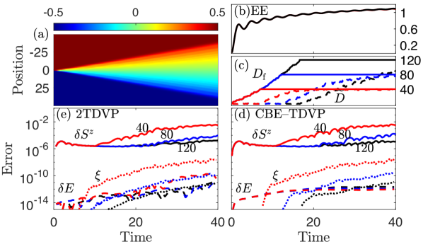
Figure 1: 100-site XX spin chain: Time evolution of a domain wall, computed with time step ${\delta}=0.05$ and U$(1)$ spin symmetry. (a) Local magnetization profile $S^{z}_{\ell}(t)$. (b) Entanglement entropy EE$(t)$ between the left and the right half of the chain. (c) Bond dimension $D_{\mathrm{f}}(t)$ and its pre-trimming expansion $\widetilde{D}(t)$ per time step, for $D_{\mathrm{max}}\!=\!120$. (d,e) Error analysis: magnetization $\delta S^{z}(t)$ (solid line),i.e., the maximum deviation (over $\ell$) of $S_{\ell}^{z}(t)$ from the exact result, , energy $\delta E(t)$ (dashed line), and discarded weight $\xi(t)$ (dotted line) for $D_{\mathrm{max}}\!=\!40$ (red), $80$ (blue) and $120$ (black), computed with (d) CBE–TDVP or (e) 2TDVP. Remarkably, the errors are comparable in size, although CBE–TDVP has much smaller computational costs.

Results.— We now benchmark CBE–TDVP for three spin models, then illustrate its performance for large $d$ using the Peierls–Hubbard model with $d=36$. Our benchmark comparisons track the time evolution of the entanglement entropy EE($t$) between the left and right halves of a chain, the bond dimensions $D_{\mathrm{f}}(t)$ and $\widetilde{D}(t)$, the discarded weight $\xi(t)$, the deviations from exact results of spins expectation values, $\delta S(t)$, and the energy change, $\delta E(t)$, which should vanish for unitary time evolution.

XX model: domain wall motion.— We consider a spin chain with Hamiltonian $H_{\mathrm{XX}}=\sum_{\ell}(S^{x}_{\ell}S^{x}_{\ell+1}+S^{y}_{\ell}S^{y}_{\ell+1})$. We compute the time evolution of the local magnetization profile $S^{z}_{\ell}(t)=\braket{\Psi(t)}{\widehat{S}_{\ell}^{z}}{\Psi(t)}$, initialized with a sharp domain wall, $\ket{\Psi(0)}\!=\!\ket{\uparrow\uparrow\!\ldots\!\uparrow\downarrow\downarrow\!\ldots\!\downarrow}$. For comparison, the analytical solution for ${\mbox{\small$\mathscr{L}$}}\to\infty$ reads [60] $S^{z}_{\ell}(t)=-1/2\sum_{n=1-\ell}^{\ell-1}J_{n}(t)^{2}$, for $\ell\geq 1$ (right half) and $S^{z}_{\ell}=-S^{z}_{1-\ell}$ otherwise, where $J_{n}(t)$ is the Bessel function of the first kind. The domain wall spreads with time [Fig. 1(a)], entailing a steady growth of the entanglement entropy (EE) between the left and right halves of the spin chain [Fig. 1(b)]. $D(t)$ and $\widetilde{D}(t)$ [Fig. 1(c)] start from 1 and 0. Initially, $\widetilde{D}$ remains remarkably small ($\lesssim 10$), while $D_{\mathrm{f}}$ increases in steps of $\widetilde{D}$ until reaching $D_{\mathrm{max}}$. Thereafter $\widetilde{D}$ increases noticeably, but remains below $D_{\mathrm{max}}$ for all times shown here. This reflects CBE frugality—bonds are expanded only as much as needed.

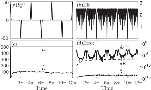
Figure 2: 100-site one-axis twisting model: Time evolution of an initially $x$-polarized spin state, computed using ${\delta}=0.01$ and $\mathbb{Z}_{2}$ spin symmetry. (a) Total spin $S^{\rm{tot}}_{x}(t)$, (b) entanglement entropy, and (c) bond dimensions. (d) Error analysis: error in total spin density $\delta s^{\rm{tot}}_{x}(t)$ (solid line), energy $\delta E(t)$ (dashed line), and discarded weight $\xi(t)$ (dotted line), for $D_{\mathrm{max}}=500$.

Figure 1(d) illustrates the effects of changing $D_{\mathrm{max}}$, following the error analysis of Ref. 61. The leading error is quantified by $\delta S^{z}(t)$ (solid line), the maximum deviation (over $\ell$) of $S_{\ell}^{z}(t)$ from the exact result. Comparing the data for $D_{\mathrm{max}}=40,80,120$, we observe a finite bond dimension effect: The error $\delta S^{z}$ increases appreciably once the discarded weight $\xi$ (dotted line) becomes larger than $10^{-11}$. By contrast, the energy change (dashed line) stays small irrespective of the choice of $D_{\mathrm{max}}$. (For more discussion of error accumulation, see Ref. [56].) Figure 1(e) shows a corresponding error analysis for 2TDVP, computed using $D\!=\!D_{\mathrm{max}}$; its errors are comparable to those of CBE–TDVP, though the latter is much cheaper.

One-axis twisting (OAT) model: quantum revivals.— The OAT model has a very simple Hamiltonian, $H_{\mathrm{OAT}}=(\sum_{\ell}S^{z}_{\ell})^{2}/2$, but its long-range interactions are a challenge for tensor network methods using real-space parametrizations. We study the evolution of $S^{\mathrm{tot}}_{x}(t)=\bra{\Psi(t)}\sum_{\ell}\widehat{S}^{x}_{\ell}\ket{\Psi(t)}$, for an initial $\ket{\Psi(0)}$ having all spins $x$-polarized (an MPS with $D=1$). The exact result, $S^{\rm{tot}}_{x}(t)=(L/2){\rm{cos}}^{L-1}(t/2)$, exhibits periodic collapses and revivals [62]. Yang and White [50] have studied the short-time dynamics using TDVP with global subspace expansion, reaching times $t\leq 0.5$. CBE–TDVP is numerically stable for much longer times [Fig. 2(a)]; it readily reached $t=12\pi$, completing three cycles. (More would have been possible with linear increase in computation time.) This stability is remarkable, since the rapid initial growth of the entanglement entropy, the finite time-step size, and the limited bond dimension [Fig. 2(b,c)] cause some inaccuracies, which remain visible throughout [Fig. 2(d)]. However, such numerical noise evidently does not accumulate over time and does not spoil the long-time dynamics: CBE–TDVP retains the treasured properties (i-iv) of 1TDVP, up to the truncation tolerance governed by $\xi$.

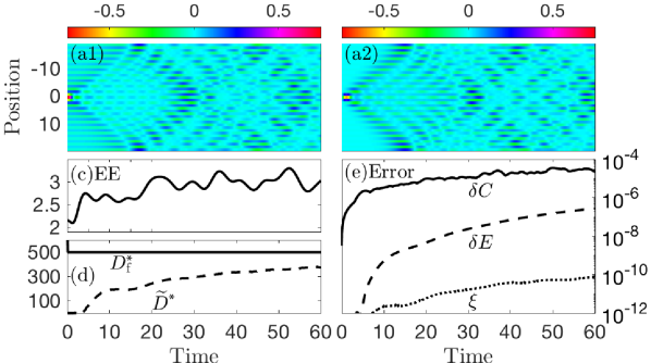
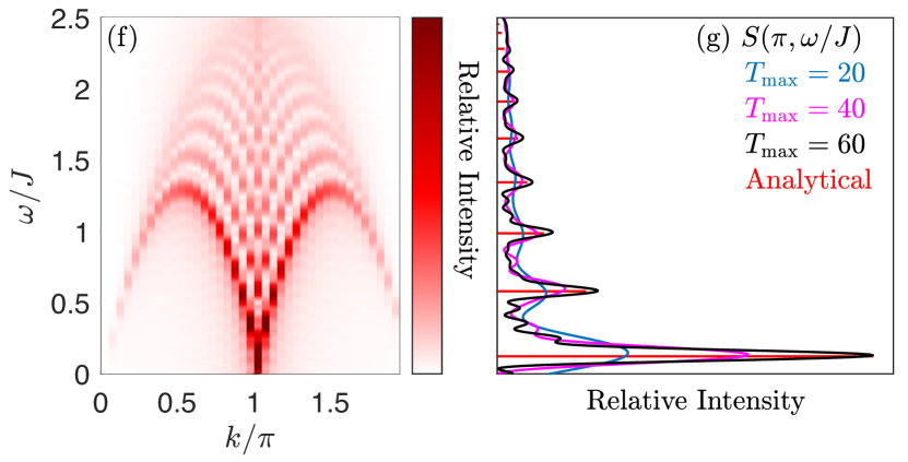
Figure 3: 40-site SU(2) Haldane-Shastry model: (a-d) Time evolution of a spin excitation, computed with ${\delta}=0.05$ and SU$(2)$ spin symmetry. (a1,a2) Real and imaginary parts of $C(x,t)$, (b) entanglement entropy, and (c) bond dimensions. (d) Error analysis: $\delta C(t)$, the maximum of $\delta C(x,t)$ over $x$ (solid line), energy $\delta E(t)$ (dashed line) and discarded weight $\xi(t)$ (dotted line), for $D_{\mathrm{max}}=500$. (f) Normalized spectral function $S(k,\omega)/S(\pi,0)$, obtained using $t_{\mathrm{max}}=60$. (g) $S(\pi,\omega)/S(\pi,0)$, obtained using $t_{\mathrm{max}}=20,40$, $60$; red lines indicate exact peak heights.

$\rm{SU}(2)$ Haldane-Shastry model: spectral function.— Our final benchmark example is the SU$(2)$ Haldane-Shastry model on a ring of length $\mathscr{L}$, with Hamiltonian

$$H_{\textrm{HS}}=J\sum_{\ell<\ell^{\prime}\leq{\scriptscriptstyle\!\mathscr{L}}}\frac{\pi^{2}{\bf{S}}_{\ell}\cdot{\bf{S}}_{\ell^{\prime}}}{{\mbox{\small$\mathscr{L}$}}^{2}{\rm{sin}}^{2}\frac{\pi}{{\scriptscriptstyle\!\mathscr{L}}}(\ell-\ell^{\prime})}.$$ (11)

Its ground state correlator, $C(x,t)\!=\!\braket{\Psi_{0}}{\widehat{\bf{S}}_{x}(t)\widehat{\bf{S}}_{0}(0)}{\Psi_{0}}$, is related by discrete Fourier transform to its spectral function, $S(k,\omega)$, given by ($0<\ell^{\prime}<\ell\leq{\mbox{\small$\mathscr{L}$}}/2$) [63, 64]

$$S\!\left(2(\ell+\ell^{\prime})\tfrac{\pi}{{\scriptscriptstyle\!\mathscr{L}}},\tfrac{\pi^{2}}{{\scriptscriptstyle\!\mathscr{L}}^{2}}((\ell+\ell^{\prime}){\mbox{\small$\mathscr{L}$}}-2(\ell^{2}+{\ell^{\prime}}^{2})+\ell-\ell^{\prime})\right)$$ (12)

$$\quad=\frac{2\ell-2\ell^{\prime}-1}{(2\ell-1)({\mbox{\small$\mathscr{L}$}}-2\ell^{\prime}-1)}\prod_{\overline{\ell}=\ell^{\prime}+1}^{\ell-1}\frac{2\overline{\ell}({\mbox{\small$\mathscr{L}$}}-2\overline{\ell})}{(2\overline{\ell}-1)({\mbox{\small$\mathscr{L}$}}-2\overline{\ell}-1)}.$$

Figures 3(a,b) show the real and the imaginary parts of $C(x,t)$, computed using CBE–TDVP. For early times ($t\leq 20$), the local excitation introduced at $\ell=0$, $t=0$ spreads ballistically, as reported previously [65, 66, 28]. Once the counter-propagating wavefronts meet on the ring, an interference pattern emerges. Our numerical results remain accurate throughout, as shown by the error analysis in Fig. 3(e). Figure 3(f) shows the corresponding spectral function $S(k,\omega)$, obtained by discrete Fourier transform of $C(x,t)$ using a maximum simulation time of $t_{\mathrm{max}}$. Figure 3(g) shows a cut along $k\!=\!\pi$: peaks can be well resolved by increasing $t_{\mathrm{max}}$, with relative heights in excellent agreement with the exact Eq. (12).

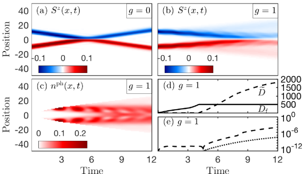
Figure 4: Peierls–Hubbard model: Real-space scattering of two electron wave packets, for $U\!=\!10$ and $\omega_{\mathrm{ph}}\!=\!3$, computed with ${\delta}=0.05$, $n_{\mathrm{max}}^{\mathrm{ph}}\!=\!=8$ and U(1) spin symmetry. (a,b) Spin magnetic moment $S^{z}(x,t)$ for $g\!=\!0$ and $g\!=\!1$. (c) Phonon density $n^{\mathrm{ph}}(x,t)$, (d) bond dimensions, and (e) error analysis: energy $\delta E(t)$ (dashed line) and discarded weight $\xi(t)$ (dotted line), all computed for $g\!=\!1$, with $D_{\mathrm{max}}=500$.

Peierls–Hubbard model:​ scattering dynamics.— Finally, we consider the scattering dynamics of interacting electrons coupled to phonons. This interaction leads to non-trivial low-energy physics involving polarons [67, 68, 69, 70, 71, 72, 73, 74, 75, 76, 77, 78, 79]; the numerical study of polaron dynamics is currently attracting increasing attention [69, 80, 81, 82, 83, 84]. Here, we consider the 1-dimensional Peierls–Hubbard model,

$$H_{\textrm{PH}} =\sum_{\ell}Un_{\ell\uparrow}n_{\ell\downarrow}+\sum_{\ell}\omega_{\mathrm{ph}}b^{\dagger}_{\ell}b^{\vphantom{dagger}}_{\ell}$$ (13)

$$\;\;+\sum_{\ell\sigma}(c^{\dagger}_{\ell\sigma}c^{\vphantom{dagger}}_{{\ell+1}\sigma}\!+\!\mathrm{h.c.})\bigl{(}-t+b^{\dagger}_{\ell}\!+\!b^{\vphantom{dagger}}_{\ell}\!-\!b^{\dagger}_{{\ell+1}}\!-\!b_{{\ell+1}}\bigr{)}\,.$$

Spinful electrons with onsite interaction strength $U$ and hopping amplitude $t\!=\!1$, and local phonons with frequency $\omega_{\mathrm{ph}}$, are coupled with strength $g$ through a Peierls term modulating the electron hopping.

We consider two localized wave packets with opposite spins, average momenta $k=\pm\pi/2$ and width $W$ [85, 86], initialized as $\ket{\Psi_{\pm}}=\sum_{\ell}Ae^{-(\frac{x_{\ell}\mp x_{0}}{W})^{2}}e^{\mp\mathrm{i}kx_{\ell}}c_{\ell\pm}^{\dagger}\ket{0}$, where $\ket{0}$ describes an empty lattice. Without electron-phonon coupling [$g=0$, Fig. 4(a)], there is little dispersion effect through the time of flight, and the strong interaction causes an elastic collision. By contrast, for a sizable coupling in the nonperturbative regime [77, 79] [$g\!=\!1$, Figs. 4(b-e)], phonons are excited by the electron motion [Fig. 4(c)]. After the two electrons have collided, they show a tendency to remain close to each other (though a finite distance apart, since $U$ is large) [Fig. 4(b)]; they thus seem to form a bi-polaron, stabilized by a significant phonon density in the central region [Fig. 4(c)].

We limited the phonon occupancy to $n^{\mathrm{ph}}_{\mathrm{max}}\!=\!8$ per site. Then, $d=4(n^{\mathrm{ph}}_{\mathrm{max}}\!+\!1)\!=\!36$, and $\overline{D}\!=\!35D_{\mathrm{f}}$ is so large that 2TDVP would be utterly unfeasible. By contrast, CBE–TDVP requires a comparatively small bond expansion of only $\widetilde{D}(t)\leq{4D_{\mathrm{max}}}$ for the times shown; after that, the discarded weight $\xi(t)$ becomes substantial [Figs. 4(d,e)].

Conclusions and outlook.— Among the schemes for MPS time evolution, 1TDVP has various advantages (see introduction), but its projection error is uncontrolled. 2TDVP remedies this, albeit at 2s costs, $\mathcal{O}(d^{2}wD^{3})$, and is able to simulate dynamics reliably [44]. CBE–TDVP at 1s costs, $\mathcal{O}(dwD^{3})$ achieves the same accuracy as 2TDVP. Moreover, CBE–TDVP comes with significantly slower growth of bond dimensions $D$ in time, which speeds up the calculations further (see Ref. [56]).

Our benchmark tests of CBE–TDVP, on three exactly solvable spin models (two with long-range interactions), demonstrate its reliability. Our results on the Peierls–Hubbard model suggest that bi-polarons form during electron scattering—an effect not previously explored numerically. This illustrates the potential of CBE–TDVP for tracking complex dynamics in computationally very challenging models.

For applications involving the time evolution of MPSs defined on “doubled” local state spaces, with effective local bond dimensions $d_{\mathrm{eff}}=d^{2}$, the cost reduction of CBE–TDVP vs. 2TDVP, $\mathcal{O}(d^{2}wD^{3})$ vs. $\mathcal{O}(d^{4}wD^{3})$, will be particularly dramatic. Examples are finite temperature properties, treated by purification of the density matrix [87] or dissipation-assisted operator evolution [88]; and the dynamics of open quantum systems [89], described by Liouville evolution of the density matrix [90, 91, 92] or by an influence matrix approach [93].

We thank Andreas Weichselbaum and Frank Pollmann for stimulating discussions, and Seung-Sup Lee, Juan Espinoza, Matan Lotem, Jeongmin Shim and Andreas Weichselbaum for helpful comments on our manuscript. Our computations employed the QSpace tensor library [94, 95]. This research was funded in part by the Deutsche Forschungsgemeinschaft under Germany’s Excellence Strategy EXC-2111 (Project No. 390814868), and is part of the Munich Quantum Valley, supported by the Bavarian state government through the Hightech Agenda Bayern Plus.

Supplemental material: Time-dependent variational principle with controlled bond expansion for matrix product states

S-1 Single site (fixed rank) tangent space projector

The structure (7) of the tangent space projector $\mathcal{P}^{1\mathrm{s}}$ can be motivated by the following short-cut argument (equivalent to invoking gauge invariance [21, 22]). If $\Psi$ is represented as an MPS, then its tangent vectors $\delta\Psi$ under the fixed-rank approximation can be expressed as a sum of MPSs each containing one derivative of a local tensor. This representation is not unique, but its gauge redundancy can be easily removed. To do so, let us first consider the variation of MPS in Eq. (1) on a single bond $\ell$, i.e., $A_{\ell}C_{\ell+1}\!=\!A_{\ell}\Lambda_{\ell}B_{\ell+1}$, while the other tensors remain fixed (and hence are not depicted below). Its first order variation then gives us $\delta A_{\ell}\Lambda_{\ell}B_{\ell+1}+A_{\ell}\delta\Lambda_{\ell}B_{\ell+1}+A_{\ell}\Lambda_{\ell}\delta B_{\ell+1}$. By further rewriting $\delta A_{\ell}\Lambda_{\ell}$ as $A_{\ell}\Lambda^{\prime}_{\ell}+{\overline{A}}_{\ell}{\overline{\Lambda}}{}^{\prime}_{\ell}$ and $\Lambda_{\ell}\delta B_{\ell+1}$ as $\Lambda^{\prime\prime}_{\ell}B_{\ell+1}+{\overline{\Lambda}}{}^{\prime\prime}_{\ell}{\overline{B}}_{\ell+1}$, we obtain the following unique decomposition,

$$\raisebox{-7.11317pt}{\includegraphics[width=382.88454pt]{Eq/LocalVariationOfPsi}},$$ (S1)

with ${\widetilde{\Lambda}}_{\ell}=\Lambda^{\prime}_{\ell}+\delta\Lambda_{\ell}+\Lambda^{\prime\prime}_{\ell}$. The three terms on the right are mutually orthogonal to each other. Each of them belongs to the image space of one of the following three orthogonal projectors:

$$\raisebox{-9.10486pt}{\includegraphics[width=187.75687pt]{Eq/LocalVariationProjectorSimplified}}\,;$$ (S2)

their sum is a tangent space projector for $A_{\ell}\Lambda_{\ell}B_{\ell+1}$. Repeating the same argument for all the bonds, while avoiding double counting, i.e., including every term only once, we readily obtain $\mathcal{P}^{1\mathrm{s}}$ given by the second line of Eq. (7).

Therefore, given an MPS of the form (1), $\mathcal{P}^{1\mathrm{s}}$ is indeed the orthogonal projector onto its tangent space under the fixed-rank approximation. For real-time evolution, applying the Hamiltonian to $\ket{\Psi}$ leads the state out of its tangent space. In the 1TDVP scheme, $H\ket{\Psi}$ is approximated by $\mathcal{P}^{1\mathrm{s}}H\ket{\Psi}$, its orthogonal projection onto the tangent space, leading to Eq. (6).

S-2 Analysis of CBE-TDVP error propagation

The TDVP time evolution of an MPS under the fixed-rank approximation is unitary, with energy conservation if the Hamiltonian is time-independent. Expanding the tangent space does not spoil these desirable properties, provided that no truncations are performed. However, then the bond dimension would keep growing with time, which is not practical for studies of long-time dynamics.

With our CBE approach, we instead restrict the bond dimension growth by bond trimming using $\epsilon=10^{-12}$, and also stopping the increase of $D_{\mathrm{f}}$ once it has reached a specified maximal value $D_{\mathrm{max}}$. Due to these truncations, the desirable TDVP properties are no longer satisfied exactly. However, for each time step they do hold within the truncation error, as shown by Ceruti, Kusch, and Lubich [51]. Thus, the time evolution per time step is almost unitary. Nevertheless, errors can accumulate with time, hence it is unclear a priori to what extent the desirable TDVP properties survive over long times.

To investigate this, we revisit our first benchmark example for the domain wall motion of the XX model. We use CBE–TDVP (while exploiting $U(1)$ spin symmetry) to compute the forward-backward fidelity [Fig. S-1(a)]

$$F(\bar{t})=|\!\braket{\Psi_{-}(\bar{t})}{\Psi_{+}(t)}\!|^{2}\,,\quad\bar{t}\!=\!t_{\mathrm{max}}\!-\!t\in[0,t_{\mathrm{max}}]\,.$$ (S3)

Here, $\ket{\Psi_{+}(t)}\!=\!e^{-\mathrm{i}Ht}\ket{\Psi(0)}$ is obtained through forward evolution for time $t$, and $\ket{\Psi_{-}(\bar{t})}\!=\!e^{\mathrm{i}H\bar{t}}\ket{\Psi_{+}(t_{\mathrm{max}})}$ through forward evolution until time $t\!=\!t_{\mathrm{max}}$, then back-evolution for $\bar{t}\!=\!t_{\mathrm{max}}\!-\!t$ to get back to time $t$. The deviation of the fidelity from unity, $\delta F(\bar{t})\!=\!1\!-\!F(\bar{t})$, equals zero for unitary evolution; increases with $\bar{t}$ if time evolution is computed using truncations; and tends to 1 for $\bar{t}\to t_{\mathrm{max}}$ if truncations are too severe.

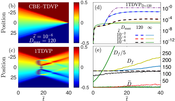
Figure S-1: (a) Forward-backward time evolution for the computation of $F(t)$. (b,c) Back-evolution of the domain wall, described by $\ket{\Psi_{-}(\bar{t})}$, computed using (b) CBE–TDVP and (c) 1TDVP. (d) Time evolution of $\delta F(\bar{t})=1-F(\bar{t})$, computed via 1TDVP with $D=120$ (dash-dotted line), and via CBE–TDVP using three values of $\widetilde{\epsilon}$, and either with $D_{\rm{max}}\!=\!120$ (dashed lines) or $D_{\rm{max}}\!=\!\infty$ (solid lines). (e) Time evolution of the corresponding bond dimensions $D_{\mathrm{f}}(\bar{t})$ (solid lines) and $\widetilde{D}(\bar{t})$ (dots). (The solid green curve shows $D_{\mathrm{f}}/5$.)

Figure 1(b) shows the back-evolution of the domain wall described by $\ket{\Psi_{-}(\bar{t})}$ as $\bar{t}$ increases from $0$ to $t_{\mathrm{max}}=40$, where both $\ket{\Psi_{+}(t)}$ and $\ket{\Psi_{-}(\bar{t})}$ were computed using CBE–TDVP with the truncation parameters stated in the main text, namely $\widetilde{\epsilon}\!=\!10^{-6}$ and $D_{\mathrm{max}}\!=\!120$. The corresponding $\delta F(\bar{t})$ (Fig. 1(d), black dashes) shows initial transient growth, but then saturates at a remarkably small plateau value of $6.7\times 10^{-5}$. Moreover, the corresponding bond expansion per update, $\widetilde{D}(\bar{t})$ (Fig. 1(e), black dots), increases only fairly slowly. For these truncation settings, the CBE–TDVP errors are thus clearly under good control and do not accumulate rapidly, so that long-time evolution can be computed accurately.

The fidelity becomes worse ($\delta F(\bar{t})$ increases) if the singular-value threshold for bond expansion, $\widetilde{\epsilon}$, is raised (Fig. 1(d), dashed lines). Nevertheless, even for $\widetilde{\epsilon}$ as large as $10^{-2}$ we find long-time plateau behavior for $\delta F(\bar{t})$, implying that the errors remain controlled. This illustrates the robustness of CBE–TDVP. The plateau value can be decreased by increasing $D_{\mathrm{max}}$, but the reduction becomes significant only if $\widetilde{\epsilon}$ is sufficiently small. Even for $D_{\mathrm{max}}\!=\!\infty$ (Fig. 1(d), solid lines) the plateau reduction relative to $D_{\mathrm{max}}\!=\!120$ is modest, whereas the corresponding growth in $D_{\mathrm{f}}$ (Fig. 1(e), solid lines) becomes so rapid that this setting is not recommended in practice.

Finally, Figs. 1(c) and 1(d) (dash-dotted, purple line) also show 1TDVP results, computed with $D=120$: the domain wall fails to recontract to a point, and the fidelity reaches zero ($\delta F(\bar{t})$ reaches $1$). This occurs even though 1TDVP uses no truncations besides the tangent space projection, and hence yields unitary time evolution. This poor performance illustrates a key limitation of 1TDVP when exploiting symmetries (as here): time evolution involves transitions to sectors having quantum numbers not yet present, but 1TDVP  cannot include these, due to the fixed-rank nature of its tangent space projection. CBE–TDVP by construction lifts this restriction.

S-3 Comparison of CPU time for CBE–TDVP and 2TDVP

In this section, we compare the CPU time for CBE–TDVP and 2TDVP. As a demonstration, we use the one-axis twisting (OAT) model discussed in Results in the main text. All CPU time measurements were done on a single core of an Intel Core i7-9750H processor.

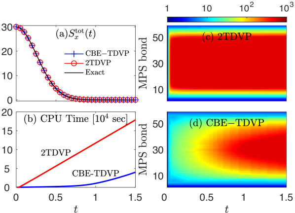
Figure S-2: $60$-site one-axis twisting model for spin $S=1/2$: Time evolution of an initially $x$-polarized spin state, computed using ${\delta}\!=\!0.01$, $D_{\mathrm{max}}\!=\!500$, and $\mathbb{Z}_{2}$ spin symmetry. (a) Total spin $S^{\rm{tot}}_{x}(t)$ for CBE–TDVP (blue), 2TDVP (red) and the exact solution (black). (b) CPU time for CBE-TDVP (blue) and 2TDVP (red). (c,d) Color scale plot of the bond dimension as a function of time for all MPS bonds, for (c) 2TDVP and (d) CBE–TDVP.

First, we compare the early-time behavior of CBE–TDVP and 2TDVP. From $t=0$ to $1.5$, both methods yield good accuracy as shown in Fig. S-2(a). The CPU time spent to achieve this, however, is quite different. In Fig. S-2(b), we see that while the 2TDVP takes about two days, CBE–TDVP accomplishes the same time span overnight.

The main reason for this difference does not lie in the 1s vs. 2s scaling of CBE–TDVP vs. 2TDVP (discussed below), because $d=2$ (for $S=1/2$) is small, and CBE involves some algorithmic overhead for determining the truncated complement ${\widetilde{A}}{}^{\mathrm{tr}}_{\ell}(\raisebox{-1.42262pt}{\includegraphics[width=16.04504pt]{Fig/TriangleOrangeA}})$. Instead, the difference reflects the fact that the growth in MPS bond dimension $D(t)$ with time is much slower for CBE-TDVP than 2TDVP. This implies dramatic cost savings, since both methods have time complexity proportional to $D^{3}$. Figure S-2(c,d) show the time evolution of bond dimensions for all MPS bonds for CBE–TDVP and 2TDVP respectively. For 2TDVP [Fig. S-2(c)], the bond dimensions grow almost exponentially and quickly saturate to their specified maximal value, here $D_{\rm{max}}=500$. This saturation is reflected by the early onset of linear growth in the CPU time in Fig. S-2(b). By contrast, the bond dimensions of CBE–TDVP show a much slower growth [Fig. S-2(d)], yielding a strong reduction in CPU time compared to 2TDVP.

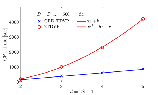
Figure S-3: CPU time per sweep for the $20$-site one-axis twisting model, computed for several values of $S$, at $D_{\rm{max}}=500$.

Second, we demonstrate that when $D$ is fixed, the time complexity of CBE–TDVP vs. 2TDVP scales as $d$ vs. $d^{2}$, implying 1s vs. 2s scaling. Figure S-3 shows this by displaying the CPU time per sweep for the OAT model for several different values of the spin $S$, with the MPS bond dimension fixed at $D_{\mathrm{max}}=500$.

References

- Dirac [1930] P. A. M. Dirac, Note on exchange phenomena in the Thomas atom, Math. Proc. Camb. Philos. Soc. 26, 376 (1930).
- McLachlan [1964] A. McLachlan, A variational solution of the time-dependent Schrodinger equation, Molecular Physics 8, 39 (1964).
- Meyer et al. [1990] H.-D. Meyer, U. Manthe, and L. Cederbaum, The multi-configurational time-dependent Hartree approach, Chem. Phys. Lett. 165, 73 (1990).
- Deumens et al. [1994] E. Deumens, A. Diz, R. Longo, and Y. Öhrn, Time-dependent theoretical treatments of the dynamics of electrons and nuclei in molecular systems, Rev. Mod. Phys. 66, 917 (1994).
- Verstraete et al. [2008] F. Verstraete, V. Murg, and J. Cirac, Matrix product states, projected entangled pair states, and variational renormalization group methods for quantum spin systems, Adv. Phys 57, 143 (2008).
- Cirac and Frank Verstraete [2009] J. I. Cirac and Frank Verstraete, Renormalization and tensor product states in spin chains and lattices, J. Phys. A Math. 42, 504004 (2009).
- Eisert et al. [2010] J. Eisert, M. Cramer, and M. B. Plenio, Colloquium: Area laws for the entanglement entropy, Rev. Mod. Phys. 82, 277 (2010).
- Schollwöck [2011] U. Schollwöck, The density-matrix renormalization group in the age of matrix product states, Ann. Phys. 326, 96 (2011).
- Stoudenmire and White [2012] E. Stoudenmire and S. R. White, Studying two-dimensional systems with the density matrix renormalization group, Annu. Rev. Condens. Matter Phys. 3, 111 (2012).
- Bridgeman and Chubb [2017] J. C. Bridgeman and C. T. Chubb, Hand-waving and interpretive dance: an introductory course on tensor networks, J. Phys. A Math. 50, 223001 (2017).
- Orús [2019] R. Orús, Tensor networks for complex quantum systems, Nat. Rev. Phys. 1, 538 (2019).
- Silvi et al. [2019] P. Silvi, F. Tschirsich, M. Gerster, J. Jünemann, D. Jaschke, M. Rizzi, and S. Montangero, The tensor networks anthology: Simulation techniques for many-body quantum lattice systems, SciPost Phys. Lect. Notes , 8 (2019).
- Koch and Lubich [2007] O. Koch and C. Lubich, Dynamical low-rank approximation, SIAM J. Matrix Anal. Appl. 29, 434 (2007).
- Koch and Lubich [2010] O. Koch and C. Lubich, Dynamical tensor approximation, SIAM J. Matrix Anal. Appl. 31, 2360 (2010).
- Haegeman et al. [2011] J. Haegeman, J. I. Cirac, T. J. Osborne, I. Pižorn, H. Verschelde, and F. Verstraete, Time-dependent variational principle for quantum lattices, Phys. Rev. Lett. 107, 070601 (2011).
- Koffel et al. [2012] T. Koffel, M. Lewenstein, and L. Tagliacozzo, Entanglement entropy for the long-range Ising chain in a transverse field, Phys. Rev. Lett. 109, 267203 (2012).
- Hauke and Tagliacozzo [2013] P. Hauke and L. Tagliacozzo, Spread of correlations in long-range interacting quantum systems, Phys. Rev. Lett. 111, 207202 (2013).
- Lubich and Oseledets [2013] C. Lubich and I. V. Oseledets, A projector-splitting integrator for dynamical low-rank approximation, BIT Numer. Math. 54, 171 (2013).
- Lubich et al. [2013] C. Lubich, T. Rohwedder, R. Schneider, and B. Vandereycken, Dynamical approximation by hierarchical Tucker and tensor-train tensors, SIAM J. Matrix Anal. Appl. 34, 470 (2013).
- Haegeman et al. [2013] J. Haegeman, T. J. Osborne, and F. Verstraete, Post-matrix product state methods: To tangent space and beyond, Phys. Rev. B 88, 075133 (2013).
- Lubich et al. [2015] C. Lubich, I. V. Oseledets, and B. Vandereycken, Time integration of tensor trains, SIAM J. Numer. Anal. 53, 917 (2015).
- Haegeman et al. [2016] J. Haegeman, C. Lubich, I. Oseledets, B. Vandereycken, and F. Verstraete, Unifying time evolution and optimization with matrix product states, Phys. Rev. B 94, 165116 (2016).
- Kieri et al. [2016] E. Kieri, C. Lubich, and H. Walach, Discretized dynamical low-rank approximation in the presence of small singular values, SIAM J. Numer. Anal. 54, 1020 (2016).
- Zauner-Stauber et al. [2018] V. Zauner-Stauber, L. Vanderstraeten, M. T. Fishman, F. Verstraete, and J. Haegeman, Variational optimization algorithms for uniform matrix product states, Phys. Rev. B 97, 045145 (2018).
- Vanderstraeten et al. [2019] L. Vanderstraeten, J. Haegeman, and F. Verstraete, Tangent-space methods for uniform matrix product states, SciPost Phys. Lect. Notes , 7 (2019).
- Bauernfeind and Aichhorn [2020] D. Bauernfeind and M. Aichhorn, Time Dependent Variational Principle for Tree Tensor Networks, SciPost Phys. 8, 24 (2020).
- Rams and Zwolak [2020] M. M. Rams and M. Zwolak, Breaking the entanglement barrier: Tensor network simulation of quantum transport, Phys. Rev. Lett. 124, 137701 (2020).
- Secular et al. [2020] P. Secular, N. Gourianov, M. Lubasch, S. Dolgov, S. R. Clark, and D. Jaksch, Parallel time-dependent variational principle algorithm for matrix product states, Phys. Rev. B 101, 235123 (2020).
- Kloss et al. [2020] B. Kloss, D. R. Reichman, and Y. B. Lev, Studying dynamics in two-dimensional quantum lattices using tree tensor network states, SciPost Phys. 9, 70 (2020).
- Ceruti et al. [2021] G. Ceruti, C. Lubich, and H. Walach, Time integration of tree tensor networks, SIAM J. Numer. Anal. 59, 289 (2021).
- Kohn and Santoro [2021] L. Kohn and G. E. Santoro, Efficient mapping for Anderson impurity problems with matrix product states, Phys. Rev. B 104, 014303 (2021).
- Van Damme et al. [2021] M. Van Damme, R. Vanhove, J. Haegeman, F. Verstraete, and L. Vanderstraeten, Efficient matrix product state methods for extracting spectral information on rings and cylinders, Phys. Rev. B 104, 115142 (2021).
- Milsted et al. [2013] A. Milsted, J. Haegeman, and T. J. Osborne, Matrix product states and variational methods applied to critical quantum field theory, Phys. Rev. D 88, 085030 (2013).
- Gillman and Rajantie [2017] E. Gillman and A. Rajantie, Topological defects in quantum field theory with matrix product states, Phys. Rev. D 96, 094509 (2017).
- Schröder and Chin [2016] F. A. Y. N. Schröder and A. W. Chin, Simulating open quantum dynamics with time-dependent variational matrix product states: Towards microscopic correlation of environment dynamics and reduced system evolution, Phys. Rev. B 93, 075105 (2016).
- del Pino et al. [2018] J. del Pino, F. A. Y. N. Schröder, A. W. Chin, J. Feist, and F. J. Garcia-Vidal, Tensor network simulation of non-Markovian dynamics in organic polaritons, Phys. Rev. Lett. 121, 227401 (2018).
- Kurashige [2018] Y. Kurashige, Matrix product state formulation of the multiconfiguration time-dependent Hartree theory, J. Chem. Phys. 149, 194114 (2018).
- Kloss et al. [2019] B. Kloss, D. R. Reichman, and R. Tempelaar, Multiset matrix product state calculations reveal mobile Franck-Condon excitations under strong Holstein-type coupling, Phys. Rev. Lett. 123, 126601 (2019).
- Xie et al. [2019] X. Xie, Y. Liu, Y. Yao, U. Schollwöck, C. Liu, and H. Ma, Time-dependent density matrix renormalization group quantum dynamics for realistic chemical systems, J. Chem. Phys. 151, 224101 (2019).
- Xu et al. [2022] Y. Xu, Z. Xie, X. Xie, U. Schollwöck, and H. Ma, Stochastic adaptive single-site time-dependent variational principle, JACS Au 2, 335 (2022).
- Vidal [2004] G. Vidal, Efficient simulation of one-dimensional quantum many-body systems, Phys. Rev. Lett. 93, 040502 (2004).
- Daley et al. [2004] A. J. Daley, C. Kollath, U. Schollwöck, and G. Vidal, Time-dependent density-matrix renormalization-group using adaptive effective Hilbert spaces, J. Stat. Mech.: Theor. Exp. P04005 (2004).
- White and Feiguin [2004] S. R. White and A. E. Feiguin, Real-time evolution using the density matrix renormalization group, Phys. Rev. Lett. 93, 076401 (2004).
- Paeckel et al. [2019] S. Paeckel, T. Köhler, A. Swoboda, S. R. Manmana, U. Schollwöck, and C. Hubig, Time-evolution methods for matrix-product states, Ann. Phys. 411, 167998 (2019).
- Hairer et al. [2006] E. Hairer, C. Lubich, and G. Wanner, Geometric Numerical Integration (Springer-Verlag, 2006).
- Kloss et al. [2018] B. Kloss, Y. B. Lev, and D. Reichman, Time-dependent variational principle in matrix-product state manifolds: Pitfalls and potential, Phys. Rev. B 97, 024307 (2018).
- Goto and Danshita [2019] S. Goto and I. Danshita, Performance of the time-dependent variational principle for matrix product states in the long-time evolution of a pure state, Phys. Rev. B 99, 054307 (2019).
- Chanda et al. [2020] T. Chanda, P. Sierant, and J. Zakrzewski, Time dynamics with matrix product states: Many-body localization transition of large systems revisited, Phys. Rev. B 101, 035148 (2020).
- Dektor et al. [2021] A. Dektor, A. Rodgers, and D. Venturi, Rank-adaptive tensor methods for high-dimensional nonlinear PDEs, J. Sci. Comput. 88, 36 (2021).
- Yang and White [2020] M. Yang and S. R. White, Time-dependent variational principle with ancillary Krylov subspace, Phys. Rev. B 102, 094315 (2020).
- Ceruti et al. [2022] G. Ceruti, J. Kusch, and C. Lubich, A rank-adaptive robust integrator for dynamical low-rank approximation, BIT Numer. Math. (2022).
- Dunnett and Chin [2021] A. J. Dunnett and A. W. Chin, Efficient bond-adaptive approach for finite-temperature open quantum dynamics using the one-site time-dependent variational principle for matrix product states, Phys. Rev. B 104, 214302 (2021).
- Hubig et al. [2018] C. Hubig, J. Haegeman, and U. Schollwöck, Error estimates for extrapolations with matrix-product states, Phys. Rev. B 97, 045125 (2018).
- Gleis et al. [2022a] A. Gleis, J.-W. Li, and J. von Delft, Controlled bond expansion for DMRG ground state search at single-site costs, arXiv:2207.14712 [cond-mat.str-el] (2022a).
- Gleis et al. [2022b] A. Gleis, J.-W. Li, and J. von Delft, Projector formalism for kept and discarded spaces of matrix product states, arXiv:2207.13161 [quant-ph] (2022b).
- [56] See Supplemental Material at [url] for: (S-1) an explanation of the structure of the tangent space projector ; (S-2) an analysis of the fidelity of CBE–TDVP: we show that under backward time evolution (implemented by changing the sign of ), the domain wall recontracts to a point; and (S-3) a comparison of the CPU time costs of CBE–TDVP vs. 2TDVP. The Supplemental Material includes Refs. [51, 21, 22] .
- McLachlan [1995] R. I. McLachlan, On the numerical integration of ordinary differential equations by symmetric composition methods, SIAM J. Sci. Comput 16, 151 (1995).
- [58] A first-order integrator, with error , involves a single left-to-right sweep or right-to-left sweep through the entire chain. For 1TDVP, and are adjoint operations, with , hence higher-order integrators can be obtained through symmetric compositions [57]. We use one of third order (error ): , for one time step, for the next .
- Vanhecke et al. [2021] B. Vanhecke, M. V. Damme, J. Haegeman, L. Vanderstraeten, and Frank Verstraete, Tangent-space methods for truncating uniform MPS, SciPost Phys. Core 4, 4 (2021).
- Antal et al. [1999] T. Antal, Z. Rácz, A. Rákos, and G. M. Schütz, Transport in the chain at zero temperature: Emergence of flat magnetization profiles, Phys. Rev. E 59, 4912 (1999).
- Gobert et al. [2005] D. Gobert, C. Kollath, U. Schollwöck, and G. Schütz, Real-time dynamics in spin- chains with adaptive time-dependent density matrix renormalization group, Phys. Rev. E 71, 036102 (2005).
- Dooley and Spiller [2014] S. Dooley and T. P. Spiller, Fractional revivals, multiple-Schrödinger-cat states, and quantum carpets in the interaction of a qubit with qubits, Phys. Rev. A 90, 012320 (2014).
- Yamamoto et al. [2000a] T. Yamamoto, Y. Saiga, M. Arikawa, and Y. Kuramoto, Exact dynamical structure factor of the degenerate Haldane-Shastry model, Phys. Rev. Lett. 84, 1308 (2000a).
- Yamamoto et al. [2000b] T. Yamamoto, Y. Saiga, M. Arikawa, and Y. Kuramoto, Exact dynamics of the SU(K) Haldane-Shastry model, J. Phys. Soc. Japan 69, 900 (2000b).
- Haldane and Zirnbauer [1993] F. D. M. Haldane and M. R. Zirnbauer, Exact calculation of the ground-state dynamical spin correlation function of a antiferromagnetic Heisenberg chain with free spinons, Phys. Rev. Lett. 71, 4055 (1993).
- Zaletel et al. [2015] M. P. Zaletel, R. S. K. Mong, C. Karrasch, J. E. Moore, and F. Pollmann, Time-evolving a matrix product state with long-ranged interactions, Phys. Rev. B 91, 165112 (2015).
- Bonča et al. [2000] J. Bonča, T. Katrašnik, and S. A. Trugman, Mobile bipolaron, Phys. Rev. Lett. 84, 3153 (2000).
- Clay and Hardikar [2005] R. T. Clay and R. P. Hardikar, Intermediate phase of the one dimensional half-filled Hubbard-Holstein model, Phys. Rev. Lett. 95, 096401 (2005).
- Fehske and Trugman [2007] H. Fehske and S. A. Trugman, Numerical solution of the Holstein polaron problem, in Polarons in Advanced Materials, edited by A. S. Alexandrov (Springer Netherlands, Dordrecht, 2007) p. 393.
- Hague et al. [2007] J. P. Hague, P. E. Kornilovitch, J. H. Samson, and A. S. Alexandrov, Superlight small bipolarons in the presence of a strong Coulomb repulsion, Phys. Rev. Lett. 98, 037002 (2007).
- Hardikar and Clay [2007] R. P. Hardikar and R. T. Clay, Phase diagram of the one-dimensional Hubbard-Holstein model at half and quarter filling, Phys. Rev. B 75, 245103 (2007).
- Tezuka et al. [2007] M. Tezuka, R. Arita, and H. Aoki, Phase diagram for the one-dimensional Hubbard-Holstein model: A density-matrix renormalization group study, Phys. Rev. B 76, 155114 (2007).
- Fehske et al. [2008] H. Fehske, G. Hager, and E. Jeckelmann, Metallicity in the half-filled Holstein-Hubbard model, Europhys Lett. 84, 57001 (2008).
- Marchand et al. [2010] D. J. J. Marchand, G. De Filippis, V. Cataudella, M. Berciu, N. Nagaosa, N. V. Prokof’ev, A. S. Mishchenko, and P. C. E. Stamp, Sharp transition for single polarons in the one-dimensional Su-Schrieffer-Heeger model, Phys. Rev. Lett. 105, 266605 (2010).
- Hohenadler and Assaad [2013] M. Hohenadler and F. F. Assaad, Excitation spectra and spin gap of the half-filled Holstein-Hubbard model, Phys. Rev. B 87, 075149 (2013).
- Hohenadler [2016] M. Hohenadler, Interplay of site and bond electron-phonon coupling in one dimension, Phys. Rev. Lett. 117, 206404 (2016).
- Sous et al. [2018] J. Sous, M. Chakraborty, R. V. Krems, and M. Berciu, Light bipolarons stabilized by Peierls electron-phonon coupling, Phys. Rev. Lett. 121, 247001 (2018).
- Reinhard et al. [2019] T. E. Reinhard, U. Mordovina, C. Hubig, J. S. Kretchmer, U. Schollwöck, H. Appel, M. A. Sentef, and A. Rubio, Density-matrix embedding theory study of the one-dimensional Hubbard–Holstein model, J. Chem. Theory Comput. 15, 2221 (2019).
- Nocera et al. [2021] A. Nocera, J. Sous, A. E. Feiguin, and M. Berciu, Bipolaron liquids at strong Peierls electron-phonon couplings, Phys. Rev. B 104, L201109 (2021).
- Golež et al. [2012] D. Golež, J. Bonča, and L. Vidmar, Dissociation of a Hubbard-Holstein bipolaron driven away from equilibrium by a constant electric field, Phys. Rev. B 85, 144304 (2012).
- Werner and Eckstein [2013] P. Werner and M. Eckstein, Phonon-enhanced relaxation and excitation in the Holstein-Hubbard model, Phys. Rev. B 88, 165108 (2013).
- Chen et al. [2015] L. Chen, Y. Zhao, and Y. Tanimura, Dynamics of a one-dimensional Holstein polaron with the hierarchical equations of motion approach, J. Phys. Chem. Lett. 6, 3110 (2015).
- Fetherolf et al. [2020] J. H. Fetherolf, D. Golež, and T. C. Berkelbach, A unification of the Holstein polaron and dynamic disorder pictures of charge transport in organic crystals, Phys. Rev. X 10, 021062 (2020).
- Pandey et al. [2021] B. Pandey, G. Alvarez, and E. Dagotto, Excitonic wave-packet evolution in a two-orbital Hubbard model chain: A real-time real-space study, Phys. Rev. B 104, L220302 (2021).
- Al-Hassanieh et al. [2008] K. A. Al-Hassanieh, F. A. Reboredo, A. E. Feiguin, I. González, and E. Dagotto, Excitons in the one-dimensional Hubbard model: A real-time study, Phys. Rev. Lett. 100, 166403 (2008).
- Moreno et al. [2013] A. Moreno, A. Muramatsu, and J. M. P. Carmelo, Charge and spin fractionalization beyond the Luttinger-liquid paradigm, Phys. Rev. B 87, 075101 (2013).
- Verstraete et al. [2004a] F. Verstraete, J. J. Garcia-Ripoll, and J. I. Cirac, Matrix product density operators: Simulation of finite-temperature and dissipative systems, Phys. Rev. Lett. 93, 207204 (2004a).
- Rakovszky et al. [2022] T. Rakovszky, C. W. von Keyserlingk, and F. Pollmann, Dissipation-assisted operator evolution method for capturing hydrodynamic transport, Phys. Rev. B 105, 075131 (2022).
- Weimer et al. [2021] H. Weimer, A. Kshetrimayum, and R. Orús, Simulation methods for open quantum many-body systems, Rev. Mod. Phys. 93, 015008 (2021).
- Lindblad [1976] G. Lindblad, On the generators of quantum dynamical semigroups, Comm. Math. Phys. 48, 119 (1976).
- Verstraete et al. [2004b] F. Verstraete, J. J. García-Ripoll, and J. I. Cirac, Matrix product density operators: Simulation of finite-temperature and dissipative systems, Phys. Rev. Lett. 93, 207204 (2004b).
- Zwolak and Vidal [2004] M. Zwolak and G. Vidal, Mixed-state dynamics in one-dimensional quantum lattice systems: A time-dependent superoperator renormalization algorithm, Phys. Rev. Lett. 93, 207205 (2004).
- Lerose et al. [2021] A. Lerose, M. Sonner, and D. A. Abanin, Influence matrix approach to many-body floquet dynamics, Phys. Rev. X 11, 021040 (2021).
- Weichselbaum [2012] A. Weichselbaum, Non-Abelian symmetries in tensor networks: A quantum symmetry space approach, Ann. Phys. 327, 2972 (2012).
- Weichselbaum [2020] A. Weichselbaum, X-symbols for non-Abelian symmetries in tensor networks, Phys. Rev. Res. 2, 023385 (2020).