A multiplicity-preserving crossover operator on graphs

Abstract.

Evolutionary algorithms usually explore a search space of solutions by means of crossover and mutation. While a mutation consists of a small, local modification of a solution, crossover mixes the genetic information of two solutions to compute a new one. For model-driven optimization (MDO), where models directly serve as possible solutions (instead of first transforming them into another representation), only recently a generic crossover operator has been developed. Using graphs as a formal foundation for models, we further refine this operator in such a way that additional well-formedness constraints are preserved: We prove that, given two models that satisfy a given set of multiplicity constraints as input, our refined crossover operator computes two new models as output that also satisfy the set of constraints.

1. Introduction

Model-driven optimization (MDO) performs optimization directly on domain-specific models. Early motivation for developing MDO has been that modeling allows for a very expressive representation of optimization problems and their solutions across different domains; at the same time, it allows expressing problems and solutions in domain-specific (modeling) languages, potentially making optimization more accessible for domain experts, e.g., (Burton et al., 2012; Burton and Poulding, 2013; Hegedüs et al., 2015). Furthermore, the explicit representation as a model enables one to leverage domain knowledge to explore the search space more effectively (Hegedüs et al., 2015; Zschaler and Mandow, 2016). While already been used in (Hegedüs et al., 2015), there has been increased awareness recently that MDO makes the search and its employed operators amenable to the application of formal methods: exploiting the formal grounding that graphs, graph transformations, and logics on graphs provide for models, their transformations, and their properties, properties of search operators or the whole search process can be tested or even formally verified (Burdusel et al., 2021; Horcas et al., 2022; Taentzer et al., 2022; John et al., 2022b).

In practical applications of MDO, often evolutionary algorithms have been used to perform the actual optimization, e.g., (ben Fadhel et al., 2012; Abdeen et al., 2014; Fleck et al., 2017; Horcas et al., 2022). In an evolutionary algorithm, normally crossover and mutation drive the search (see, e.g., (Eiben and Smith, 2015)): Typically, given an objective (or fitness) function (or a set of these) that formalizes the properties to be optimized, an evolutionary algorithm starts with an initial population of randomly generated solutions. Then, until a termination condition is met, a new population is computed from the current one. For that, pairs of solutions are randomly selected from the current population, to which crossover is applied with a certain probability; solutions with high fitness have a higher chance of being selected. Crossover recombines parts of the two solutions, mixing their genetic information. After crossover, the computed offspring can additionally be subjected to mutation, where small local changes are performed. From the old population and the newly computed solutions the next population is randomly selected, again taking the fitness of individual solutions (but possibly also other considerations like maintenance of diversity) into account. An optimization problem can also be constrained, meaning that additional feasibility constraints restrict which solutions are considered to be feasible. In the context of evolutionary algorithms, various approaches have been suggested to deal with feasibility constraints (Michalewicz, 1995; Coello, 2010). These include immediately discarding infeasible solutions, developing methods to repair them, decrementing their fitness (according to the amount of violation of the feasibility constraints), or designing crossover and mutation operators in such a way that feasibility of solutions is always preserved.

In MDO, so far, model transformations have served as the primary means to perform evolutionary search (ben Fadhel et al., 2012; Abdeen et al., 2014; Hegedüs et al., 2015; Fleck et al., 2017; Burdusel et al., 2021; Horcas et al., 2022; John et al., 2022b). But, as we will argue in more detail later (see Sect. 2), performing crossover directly on models has not been adequately developed yet. Recently, a generic crossover operator on graphs, which can serve as a basis for crossover on models, has been introduced (Taentzer et al., 2022); in the following, we refer to this operator as generic crossover. When applying generic crossover to two models, it is guaranteed that the computed offspring at least conforms to the structure that is specified by the given meta-model. However, meta-models, including those that provide a syntax for the solution of optimization problems, are typically equipped with additional well-formedness (or, in this context, feasibility) constraints. The most basic and important of these are multiplicities, restricting the allowed incidence relations in instance models. The generic crossover operator does not take any feasibility constraints into account, i.e., solutions computed via crossover might violate the given constraints, even if the input solutions satisfied these. In this work, we refine the generic crossover operator from (Taentzer et al., 2022) towards secure crossover in such a way that it cannot any longer introduce violations of multiplicity constraints. Practical experience in MDO with evolutionary algorithms that are solely based on mutation as an operator shows that evolutionary search can profit if the used mutation rules cannot introduce new violations of feasibility constraints (Burdusel et al., 2021; Horcas et al., 2022; John et al., 2022b). Therefore, developing crossover of models in such a way that feasibility is preserved is a promising enterprise.

The direct contribution of this work is this refinement of an existing crossover operator on graphs in such a way that it preserves the validity of multiplicity constraints. By detailedly developing the according algorithms and formally proving their desired properties, we further substantiate the intuition that using models directly as representation of solutions of an optimization problem facilitates the reasoning about search operators and processes. It is hardly conceivable to develop a crossover operator that preserves multiplicities when models are encoded, e.g., as bit strings. A few algorithmic details are transferred to Appendix A. All proofs (and some additional results) are provided in Appendix B.

2. Related work

In this work, we develop a crossover operator on graphs that preserves multiplicities. Generally, this operator refines the one introduced in (Taentzer et al., 2022); it is also inspired by crossover operators on permutations (see, e.g., (Potvin, 1996)) to only compute one offspring. In the following, we discuss how crossover has been performed in MDO so far, and we discuss other crossover operators on graphs (or similar structures).

Crossover in MDO

In MDO, two encoding approaches have emerged: the rule- and the model-based approach (John et al., 2019). In the rule-based approach (e.g., (ben Fadhel et al., 2012; Abdeen et al., 2014; Hegedüs et al., 2015; Fleck et al., 2017; Bill et al., 2019)), the data structure on which optimization is performed is a sequence of applications of model transformation rules. Such sequences also represent models (by applying the sequence to a fixed start model). Since the chosen representation is a sequence, classic crossover operators like $k$-point or universal crossover are directly applicable. However, crossovers may result in a sequence of transformations that is not applicable to the start model. Repair techniques have been suggested to mitigate that problem: inapplicable transformations of a sequence can be discarded (Abdeen et al., 2014) or replaced by placeholders or random applicable transformations (Bill et al., 2019). These repairs, however, only serve to obtain a sequence of applicable model transformations. Whether or not the model that a sequence of transformations computes satisfies feasibility constraints remains unclear.

In the model-based approach (e.g., (Zschaler and Mandow, 2016; Burdusel et al., 2021; Horcas et al., 2022)), optimization is directly performed on models. Model transformation rules serve as mutation operators. Zschaler and Mandow have suggested that ideas from model differencing and merging could serve as basis for a crossover operator directly applicable to models (Zschaler and Mandow, 2016). However, except for a specific application in which crossover has been based on transformation rules (Horcas et al., 2022), evolutionary search on models as search space has been performed via mutation only (John et al., 2019; Burdusel et al., 2021; John et al., 2022b). To address this situation, we first developed the mentioned generic crossover operator for graph-like structures (Taentzer et al., 2022). Being generic and based on graphs, it can serve as a formal foundation for crossover operators on models, independently of their semantics or the employed modeling technology. However, its application can introduce violations of feasibility constraints.

In parallel work (John et al., 2022a), we suggest how to adapt that generic crossover operator to models from the Eclipse Modeling Framework (EMF) (Eclipse, 2022). We ensure that the results of crossover conform to the general structure of EMF models; however, we do not take additional well-formedness constraints like multiplicities into account. In a first small evaluation, evolutionary search can profit from using both crossover and mutation (compared to only using mutation) but only if violations of feasibility constraints that crossover introduced are immediately repaired. Crossover hampers search when used without repair. These results indicate that directly preserving multiplicities, like we suggest in the current work, is a promising enterprise. If possible, directly preserving constraints is a more general approach as ad hoc repair operations might not always be available.

Crossover on graphs

There are various approaches to crossover on graphs (or similar structures), more often than not with a specific semantics of the considered graphs in mind. Since we address typed graphs and multiplicity constraints, which are both very general concepts, we restrict our comparison to other crossover operators that generally work on graphs and do not depend (too much) on their assumed semantics. Crossover operators of which we are aware that can be quite generically applied to graphs are (Globus et al., 2000; Niehaus, 2004; Machado et al., 2010). In (Globus et al., 2000), connectedness properties of a graph are preserved, while in (Niehaus, 2004) heuristics are used to increase the likelihood of preserving acyclicity or certain reachability properties. In (Machado et al., 2010), no preservation of constraints is addressed. To the best of our knowledge, we are the first to formally ensure the preservation of such complex properties as multiplicities for a crossover operator on graphs.

3. Running example

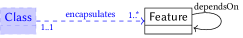
Figure 1. Metamodel (type graph) for the CRA case

The class responsibility assignment (CRA) case is an easy to grasp use case for MDO that is still practically interesting. Having been suggested as a contest problem in (Fleck et al., 2016), it continues to be used as a problem to illustrate new concepts in MDO with and to benchmark them against (Burdusel et al., 2021; John et al., 2022b).

In the CRA case, a set of Features, representing Attributes and Methods, and their interdependencies are given. It is searched for an optimal assignment of the Features to Classes. Typically, a solution is considered to be of high quality if its assignment of Features to Classes exhibits low coupling between the Classes and high cohesion inside of them; for details and a formalization of coupling and cohesion as objective functions we refer to (Fleck et al., 2016).

Fig. 1 depicts a metamodel (or type graph) that provides a syntax to represent concrete problem instances and solutions for the CRA case as models (for brevity, it is considerably simplified compared to the metamodel provided in (Fleck et al., 2016)). The black nodes serve to model problem instances, namely a set of Features and their interdependencies. The blue, dashed elements (Classes and their incident edges) serve to extend problem instances to solutions, namely to assign Features to Classes. The multiplicities serve to further prescribe which instances of the metamodel are to be considered as valid (or feasible) solutions. In our example they express that every Class should at least encapsulate one Feature ($1..*$) and that every Feature should be encapsulated by exactly one Class ($1..1$).

4. Preliminaries

In this section we present our formal preliminaries, namely graphs, computation elements with multiplicities, which serve as a formal basis for models, and the generic crossover operator that we refine in this work.

Definition 4.1 (Graph. Graph morphism).

A (directed) graph $G=(V,E,\mathit{src},\allowbreak\mathit{tar})$ consists of finite sets of nodes $V$ and edges $E$, and source and target functions $\mathit{src},\mathit{tar}\colon E\to V$.

Given two graphs $G$ and $H$, a graph morphism $f=(f_{V},f_{E})\colon G\to H$ is a pair of functions $f_{V}\colon V_{G}\to V_{H}$ and $f_{E}\colon E_{G}\to E_{H}$ such that $f_{V}(\mathit{src}_{G}(e))=\mathit{src}_{H}(f_{E}(e))$ and $f_{V}(\mathit{tar}_{G}(e))=\mathit{tar}_{H}(f_{E}(e))$ for all edges $e\in E_{G}$. A graph morphism is injective/surjective/bijective if both of its components are.

A typed graph is a graph together with a graph morphism into a fixed type graph. Intuitively, the type graph provides the available types for nodes and edges and their allowed incidence relations. Using typing to provide graphs with a richer syntax is well-established (Ehrig et al., 2006), in particular also when using typed graphs as formal basis for models (Biermann et al., 2012). For our application, however, it is advantageous to consider type graphs with more structure: Some elements of the type graph serve to model the problem that has to be optimized and others to create a solution. Encoding this distinction into the type graph has led to the definition of computation type graphs and their computation graphs (Taentzer et al., 2022; John et al., 2022b). Multiplicities allow expressing certain structural constraints (namely, lower and upper bounds on edge types) that cannot be captured by typing alone; a graph-based formalization is provided in (Taentzer and Rensink, 2005). In the following definition of a computation type graph with multiplicities and its computation graphs we bring together the definition of a type graph with multiplicities with the one of computation (type) graphs.

Definition 4.2 (Computation type graph with multiplicities. Computation graph).

A multiplicity is a pair $[i,j]\in\mathbb{N}\times(\mathbb{N}\cup\{*\})$ such that $i\leq j$ or $j=*$; $\mathit{Mult}$ denotes the set of all multiplicities. A set $X$ satisfies a multiplicity $m=[i,j]$ if $\lvert X\rvert\geq i$ and either $\lvert X\rvert\leq j$ or $j=*$; this satisfaction is denoted as $\lvert X\rvert\in m$. Via $m^{\mathrm{lb}}$ and $m^{\mathrm{ub}}$ we denote the projections to the first or second component.

A computation type graph with multiplicities is a tuple $\overline{\mathit{TG}}=(\mathit{TG}_{\mathrm{P}}\subseteq\mathit{TG},m_{\mathrm{src}},m_{\mathrm{tar}})$, where $\mathit{TG}$ is a graph, $\mathit{TG}_{\mathrm{P}}$ a designated subgraph, and $m_{\mathrm{src}},m_{\mathrm{tar}}\colon E_{\mathit{TG}}\to\mathit{Mult}$ are functions, called edge multiplicity functions. The graph $\mathit{TG}$ is called the type graph, and $\mathit{TG}_{\mathrm{P}}$ the problem type graph.

A computation graph $\overline{G}=(G,t_{G})$ over $\overline{\mathit{TG}}$ is a graph $G$ together with a graph morphism $t_{G}\colon G\to\mathit{TG}$. The intersection of $G$ with $\mathit{TG}_{\mathrm{P}}$ (in $\mathit{TG}$) is called the problem graph of $\overline{G}$ and is denoted as $G_{\mathrm{P}}$. A morphism $f\colon\overline{G}\to\overline{H}$ between computation graphs $\overline{G}=(G,t_{G})$ and $\overline{H}=(H,t_{H})$ is a graph morphism $f\colon G\to H$ such that $t_{H}\circ f=t_{G}$.

A computation graph $\overline{G}=(G,t_{G})$ typed over $\mathit{TG}$ is said to satisfy the multiplicities of a computation type graph with multiplicities $(\mathit{TG}_{\mathrm{P}}\subseteq\mathit{TG},m_{\mathrm{src}},m_{\mathrm{tar}})$ if

• for all edges $e\in E_{\mathit{TG}}$ and all nodes $p\in\{n\in V_{G}\mid t_{G}(n)=\mathit{src}_{\mathit{TG}}(e)\}$ it holds that

  $$\lvert\{e^{\prime}\in E_{G}\mid t_{G}(e^{\prime})=e\text{ and }\mathit{src}_{G}(e^{\prime})=p\}\rvert\in m_{\mathrm{tar}}(e)$$

  and

• for all edges $e\in E_{\mathit{TG}}$ and all nodes $p\in\{n\in V_{G}\mid t_{G}(n)=\mathit{tar}_{\mathit{TG}}(e)\}$ it holds that

  $$\lvert\{e^{\prime}\in E_{G}\mid t_{G}(e^{\prime})=e\text{ and }\mathit{tar}_{G}(e^{\prime})=p\}\rvert\in m_{\mathrm{src}}(e).$$

A computation graph defines a problem instance via its problem graph; (candidate) solutions are all computation graphs with coinciding problem graphs.

Definition 4.3 (Problem instance. Search space. Solution).

Given a computation type graph with multiplicities $\overline{TG}=(\mathit{TG}_{\mathrm{P}}\subseteq\mathit{TG},m_{\mathrm{src}},\allowbreak m_{\mathrm{tar}})$, a problem instance for $\overline{\mathit{TG}}$ is a computation graph $\overline{\mathit{PI}}$ over $\overline{\mathit{TG}}$. The search space $\mathcal{S}(\overline{\mathit{PI}})$ defined by $\overline{\mathit{PI}}$ consists of all computation graphs $\overline{G}$ over $\overline{\mathit{TG}}$ for which there exists (a typing-compatible) isomorphism between the problem graphs $G_{\mathrm{P}}$ and $\mathit{PI}_{\mathrm{P}}$; elements of $\mathcal{S}(\overline{\mathit{PI}})$ are called candidate solutions, or solutions for short, for the problem instance $\overline{\mathit{PI}}$. A solution is feasible if it satisfies the multiplicity constraints of $\overline{\mathit{TG}}$ and infeasible otherwise.

Example 4.4.

Formally, the metamodel for the CRA case depicted in Fig. 1 can considered to be a computation type graph with multiplicities; the black elements constitute the problem type graph; the multiplicity functions are defined by the annotations of the edges. Fig. 2 presents two feasible computation graphs $\overline{G}$ and $\overline{H}$. The typing is indicated by denoting the nodes with their types; edge types are omitted for brevity (they can unambiguously be inferred). The identifiers f1 etc. just serve to be able to speak about the individual elements. Because the problem graphs of $\overline{G}$ and $\overline{H}$ (the black Features plus edge) coincide, they constitute (feasible) solutions for the same problem instance.

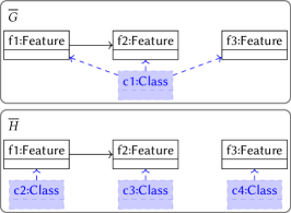
Figure 2. Two computation graphs for the CRA case that constitute solutions for the same problem instance

Summarizing, our setting is that a fixed meta-model with multiplicities provides the syntax to model different instances of an optimization problem and their solutions. In our example, the general optimization problem is the CRA case and concrete problem instances are different configurations of Features and their interdependencies for which an optimal assignment to Classes has to be found. Generally, the problem model of an instance model determines for which problem instance this model is a solution, i.e., to which search space it belongs. Evolutionary search, then, is performed for a concrete problem instance, i.e., inside of a fixed search space, which is determined by the isomorphic problem models of its members. As mentioned in Sects. 1 and 2, it is established to use model transformations (which do not change the problem part) as mutation operators during evolutionary search. This paper is concerned with developing a crossover operator that takes two solutions from the same search space as input and computes offspring solutions that belong to the same search space. At that the crossover operator shall produce feasible offsprings from feasible input.

As foundation for that, we recall the generic crossover operator that has been introduced in (Taentzer et al., 2022). There, crossover is declaratively defined and no constructive algorithm is provided; furthermore, it is defined in an abstract category-theoretic setting. Intuitively, that crossover operator prescribes that two input solutions are to be split into two parts each and these parts are to be recombined crosswise by computing a union. This results in two new solutions, also called offspring. A crossover point serves to identify elements from the two input solutions, i.e., it designates elements that are only to appear once in the union. The next definition specializes generic crossover to computation graphs.

Definition 4.5 (Generic crossover).

Given a computation type graph with multiplicities $\overline{\mathit{TG}}$, a problem instance $\overline{\mathit{PI}}$ for it, and two solutions $\overline{G}$ and $\overline{H}$ from $\mathcal{S}(\overline{\mathit{PI}})$, applying generic crossover amounts to the following:

1. Splitting: The underlying graph $G$ of $\overline{G}$ is split into two subgraphs $G_{1},G_{2}\subseteq G$ such that

   1. both $G_{1}$ and $G_{2}$ contain $G_{\mathrm{P}}$ and

   2. every element of $G$ belongs to either $G_{1}$ or $G_{2}$ (or both).

   $G_{1}$ and $G_{2}$ become computation graphs by defining their typing morphisms as the respective restrictions of $t_{G}$. The intersection $G_{\mathrm{I}}$ of $G_{1}$ and $G_{2}$ (in $G$) is called split point. The graph $H$ is split in the same way.

2. Relating $G$ and $H$ (crossover point): A further solution for $\mathit{PI}$, i.e., a computation graph $\overline{\mathit{CP}}=(\mathit{CP},t_{\mathit{CP}})$ with problem graph $\mathit{CP}_{\mathrm{P}}$ being isomorphic to $\mathit{PI}_{\mathrm{P}}$ is determined such that $\mathit{CP}$ can be considered to be a subgraph of both split points $G_{\mathrm{I}}$ and $H_{\mathrm{I}}$. Formally, this means that there are injective morphisms from $\overline{\mathit{CP}}$ to $\overline{G_{\mathrm{I}}}$ and $\overline{H_{\mathrm{I}}}$. The solution $\overline{\mathit{CP}}$ (together with the two injective morphisms) is called a crossover point.

3. Recombining: The underlying graph $G_{1}H_{2}$ of the first offspring solution $\overline{G_{1}H_{2}}$ is computed as the union of $G_{1}$ and $H_{2}$ over $\mathit{CP}$. That is, elements from $G_{1}$ and $H_{2}$ that share a preimage in $\mathit{CP}$ only appear once in the result. A typing morphism $t_{G_{1}H_{2}}\colon G_{1}H_{2}\to\mathit{TG}$ is obtained by combining the ones of $G_{1}$ and $H_{2}$; hence, a computation graph $\overline{G_{1}H_{2}}$ is computed. A second offspring solution $\overline{G_{2}H_{1}}$ is computed analogously by unifying $G_{2}$ and $H_{1}$ over $\mathit{CP}$.

The results obtained in (Taentzer et al., 2022) ensure that the two offspring solutions computed in that way are indeed solutions for the given problem model $\overline{\mathit{PI}}$: their typing morphisms are well-defined and their problem graphs are isomorphic to $\mathit{PI}_{\mathrm{P}}$ (Taentzer et al., 2022, Prop. 2). Moreover, no matter how the splits of the input graphs $G$ and $H$ are chosen, a crossover point can be found; thus, crossover is always applicable (Taentzer et al., 2022, Lem. 1). Albeit, the computed offspring does not need to satisfy the given multiplicity constraints, even if the inputs $G$ and $H$ and/or the split parts $G_{1},G_{2},H_{1},H_{2}$ do.

Example 4.6.

Figure 3 depicts two solutions that can result from applying generic crossover to the computation graphs $\overline{G}$ and $\overline{H}$ from Fig. 2. In the corresponding computations, $G$ is split such that $G_{1}$ does not contain the reference from Class c1 to Feature f3 and $G_{2}$ is the whole of $G$. Consequently, $G_{\mathrm{I}}$ coincides with $G_{1}$. Similarly, $H$ is split by omitting the reference from Class c4 to Feature f3 in $H_{1}$ and omitting Class c3 together with its reference from $H_{2}$. Consequently, $H_{\mathrm{I}}$ contains the three Classes c2, c3, c4 but only the reference from c2 to f1. As crossover point, we choose a graph that, beyond the given problem graph, contains a common preimage for Classes c1 and c2 and their respective reference to Feature f1, thus identifying them. As can be seen, the resulting offspring $\overline{G_{1}H_{2}}$ is desirable as it assigns the independent Feature f3 to its own Class. In contrast, offspring $\overline{G_{2}H_{1}}$ is infeasible, containing an empty Class (i.e., a Class with no Feature) and a multiply assigned Feature.

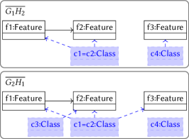
Figure 3. Two computation graphs resulting as offspring from generic crossover

We close this section with introducing some abbreviating notations and simplifying assumptions. First, we assume the problem graphs of the occurring computation graphs to be identical (and not merely isomorphic). Furthermore, from a formal point of view, morphisms (and inclusions) relate the different occurring graphs like split parts, split points, crossover points etc. Considering these explicitly leads to quite some notational overhead. To avoid that, we use common names of variables and indices to convey the relation between elements. For example, we write $x_{G}$, $x_{G_{1}}$, $x_{\mathit{PI}_{\mathrm{P}}}$, $x_{\mathit{CP}}$, etc. to indicate that the node $x_{\mathit{CP}}$ from crossover point $\mathit{CP}$ is mapped to the node $x_{\mathit{PI}_{\mathrm{P}}}$ in the problem part, the node $x_{G_{1}}$ in split part $G_{1}$ of a computation graph $G$, etc.

5. Introducing secure crossover on graphs

In this section, we introduce our crossover operator, which we call secure crossover, and prove its central properties, namely being multiplicity-preserving (feasibility-preserving) and still being able to produce any valid graph as offspring (coverage of search space). As mentioned, we develop our crossover operator as a refinement of the one introduced in (Taentzer et al., 2022) and recalled in Sect. 4. Our construction is guided by the following objectives.

1. Applied to feasible input graphs, secure crossover shall compute feasible offsprings.

2. The search space should not get unnecessarily restricted by our operator.

   At least, it should be possible to obtain every feasible graph as a result from crossover. That is, our operator should not cut off feasible regions from the search space.

3. It should be possible to perform crossover efficiently.

Finding splits of two graphs, however, and a crossover point such that both computed offspring solutions satisfy all multiplicities seems to require intensive analysis and becomes very inefficient. Therefore, we take inspiration from crossover operators that have been developed for the case where permutations (of numbers) are chosen as representation. There, to ensure that crossover of two permutations results in a permutation again, several crossover operators have been developed that only compute one offspring solution (see, e.g., (Potvin, 1996) for an overview). Analogously, in this work the basic idea is to focus entirely on one offspring solution. Computing a single feasible offspring requires significantly less computational effort than ensuring both offsprings to be feasible. We suspect that it could be cheaper to apply the operator we propose in this paper twice, instead of trying to compute an application of a crossover operator with two feasible offsprings.

Since, for formal reasons, we still want our suggested crossover operator to adhere to the definition of generic crossover, we suggest a trivial way to compute a second solution (namely, to just unify the whole given solution graphs $G$ and $H$ over the crossover point selected to compute the first offspring). However, in an implementation one would probably just omit this step as the likelihood of this second offspring being valuable is very low. Accordingly, in the following we entirely focus on the presentation of the computation of the first offspring.

In all of the following, we assume to be given two computation graphs $\overline{G}$ and $\overline{H}$ that are solutions for the same fixed problem instance $\overline{\mathit{PI}}$ (all typed over the same computation type graph with multiplicities $\overline{TG}$). We will mainly speak about their underlying graphs $G$, $H$, $\mathit{PI}$, etc. and treat their typing implicitly. Recall that $\mathit{PI}_{\mathrm{P}}$ refers to the problem graph of $\mathit{PI}$ that captures the concrete problem instance that is to be optimized.

5.1. General procedure

Our general procedure is presented in Algorithm 1 and works as follows: We construct a subgraph $G_{\mathrm{sub}}$ of $G$ as a first split part in such a way that $G_{\mathrm{sub}}$ is always feasible when $G$ is (line 1). Knowing $G_{\mathrm{sub}}$, we construct $H_{\mathrm{sub}}$ (as a second split part of $H$) and a crossover point $\mathit{CP}$ in parallel, monitoring that applying crossover with that data is not going to introduce new violations of the multiplicity constraints (lines 2–4). Computing the crossover point $\mathit{CP}$ and $H_{\mathrm{sub}}$ simultaneously allows for a much easier handling of the upper bound of the multiplicities: Whenever a node is included into $\mathit{CP}$, all edges that attach to that node’s counterparts in $G_{\mathrm{sub}}$ and $H_{\mathrm{sub}}$ will be present in the offspring, attached to that node from $\mathit{CP}$. This can lead to the resulting amount of edges being higher than the multiplicity permits. If we were to compute $H_{\mathrm{sub}}$ first, we would therefore not be able to ensure that a later choice of $\mathit{CP}$ could not lead to any breach of a maximum. These breaches would either need to be avoided when computing $\mathit{CP}$, which might not always be possible, or we would be forced to alter $G_{\mathrm{sub}}$ and $H_{\mathrm{sub}}$, creating a lot of additional computational effort. This can be avoided by selecting $\mathit{CP}$ alongside the subgraph $H_{\mathrm{sub}}$. Finally, the offspring solution $O_{1}$ is computed as the union of $G_{\mathrm{sub}}$ and $H_{\mathrm{sub}}$ over $\mathit{CP}$ (line 5). As already mentioned, to still comply with generic crossover, we formally also compute a second offspring $O_{2}$ as the union of $G$ and $H$ over $\mathit{CP}$; however, we do not expect to perform this computation in practice.

Algorithm 1 secureCrossover($G,H,\mathit{PI}_{\mathrm{P}}$)

1:$G_{\mathrm{sub}}\leftarrow$ createGsub($G,\mathit{PI}_{\mathrm{P}}$)

2:global $\mathit{CP},H_{\mathrm{sub}}\leftarrow\mathit{PI}_{\mathrm{P}}$

3:constructCP($G_{\mathrm{sub}},H$)

4:processFreeNodes($G_{\mathrm{sub}},H,H_{\mathrm{sub}})$

5:$O_{1}\leftarrow G_{\mathrm{sub}}\cup_{\mathit{CP}}H_{\mathrm{sub}}$

6:$O_{2}\leftarrow G\cup_{\mathit{CP}}H$

5.2. Creating $G_{\mathrm{sub}}$

The creation of $G_{\mathrm{sub}}$ is detailed in Algorithm 2. We initialize $G_{\mathrm{sub}}$ with $\mathit{PI}_{\mathrm{P}}$ as the problem graph is to be included anyhow. Then, for all remaining nodes of $G$, we check whether they are already included in $G_{\mathrm{sub}}$ (e.g., because they serve as target node for an included egde) and, if not, we randomly decide whether or not the node should be included (line 5). For included nodes, we also include adjacent edges (line 8). Both nodes and edges are understood to be included into $G_{\mathrm{sub}}$ with they same type they have in $\overline{G}$. Formally, $G_{\mathrm{sub}}$ becomes a computation graph over $\overline{TG}$ by defining its type function $t_{G_{\mathrm{sub}}}$ as restriction of $t_{G}$ to $G_{\mathrm{sub}}$. For simplicity, we leave this implicit in the pseudocode and in all of the following.

Algorithm 2 createGsub($G,\mathit{PI}_{\mathrm{P}}$)

1:$G_{\mathrm{sub}}\leftarrow\mathit{PI}_{\mathrm{P}}$

2:for all $x_{G}\in V_{G}$ do

3:   bool $\mathit{included}\leftarrow x_{G_{\mathrm{sub}}}\in V_{G_{\mathrm{sub}}}$

4:   if $!\mathit{included}$ then

5:     $\mathit{included}\leftarrow$ decideInclusion($x_{G}$)

6:   end if

7:   if $\mathit{included}$ then

8:     includeAdjacentEdges($x_{G},G$)

9:   end if

10:end for

The inclusion of edges is done by including a random set of the edges of $G$ in $G_{\mathrm{sub}}$ whose size is between the required lower and upper bound. In case it should not be possible to reach the lower bound (because this is violated in $G$) at least all the available edges are included in $G_{\mathrm{sub}}$. We provide an algorithm for this and an extended explanation in Appendix A.

Example 5.1.

In the CRA case, called for a feasible solution $G$, createGsub will always return the whole of $G$ as $G_{\mathrm{sub}}$. All Features are directly included into $G_{\mathrm{sub}}$ because they are part of the problem graph. Since the incoming encapsulates-edge has a source multiplicity of $[1,1]$, for every Feature-node the call of includeAdjacentEdges includes the incoming encapsulates-edge (that exists because of feasibility) and the Class from which it starts. Since, again by feasibility, empty Classes cannot occur, that process results in $G$.

5.3. Creating $H_{\mathrm{sub}}$ and $\mathit{CP}$

The main difficulty in constructing $H_{\mathrm{sub}}$ and $\mathit{CP}$ is that, as soon as a node $x_{\mathit{CP}}$ in the crossover point prescribes that nodes $x_{G_{\mathrm{sub}}}$ from $G_{\mathrm{sub}}$ and $x_{H_{\mathrm{sub}}}$ from $H_{\mathrm{sub}}$ are to be identified in the offspring, we need to ensure that no upper bound violations can be introduced by that identification: Even if in both $G_{\mathrm{sub}}$ and $H_{\mathrm{sub}}$ the upper bounds are satisfied, the sum of adjacent edges of a certain type of edges to $x_{G_{\mathrm{sub}}}$ in $G_{\mathrm{sub}}$ and $x_{H_{\mathrm{sub}}}$ in $H_{\mathrm{sub}}$ might exceed the upper bound of that type of edge. Constructing $H_{\mathrm{sub}}$ and $\mathit{CP}$ in parallel, we can react to that by either (i) not including too many edges in $H_{\mathrm{sub}}$, (ii) also including the edges into $\mathit{CP}$ (which reduces their number in the offspring), or (iii) dropping edges from $G_{\mathrm{sub}}$. As nodes from $\mathit{CP}$ are the sensitive issue, we start constructing $H_{\mathrm{sub}}$ and $\mathit{CP}$ along the nodes we know to appear in them – the nodes from the problem graph $\mathit{PI}_{\mathrm{P}}$; it actually suffices to start form the border of $\mathit{PI}_{\mathrm{P}}$ in $H$, namely the nodes of $\mathit{PI}_{\mathrm{P}}$ which have an adjacent edge (in $H$) to a node that does not belong to $\mathit{PI}_{\mathrm{P}}$.

Algorithm 3 constructCP($G_{\mathrm{sub}},H$)

1:queue $Q\leftarrow$ border($\mathit{PI}_{\mathrm{P}},H$)

2:while $Q$.notEmpty() do

3:   $x_{H}\leftarrow Q$.pop()

4:   for all $\mathit{dir}\in\{\mathit{src},\mathit{tar}\}$ do

5:     for all $e\in E_{\mathit{TG}}$ with $\mathit{dir}_{\mathit{TG}}(e)=t_{H}(x_{H})$ do

6:       for all $e^{\prime}_{H}\in\mathit{edges}(H,e,\mathit{dir},x_{H})$ do

7:         $y_{H}\leftarrow\overline{\mathit{dir}}(e_{H})$

8:         bool $\mathit{included}\leftarrow y_{H}\in V_{H_{\mathrm{sub}}}$

9:         if $\mathit{included}$ then

10:            bool $\mathit{edgeIncluded}\leftarrow e^{\prime}_{H}\in E_{H_{\mathrm{sub}}}$

11:            if $\mathit{edgeIncluded}$ then

12:              skip

13:            end if

14:            bool $\mathit{includedCP}\leftarrow y_{H}\in V_{\mathit{CP}}$

15:         end if

16:         if $!\mathit{included}$ then

17:            $\mathit{included}\leftarrow$ decideInclusion($y_{H}$)

18:         end if

19:         if $\mathit{included}$ then

20:            $\mathit{edgeIncluded}\leftarrow$ decideInclusion($e_{H}$)

21:            if $\mathit{edgeIncluded}$ then

22:              if $\mathit{includedCP}\land$ edgeCount($H,G,e,\overline{\mathit{dir}},y$)$+1>m_{\mathit{dir}}^{\mathrm{ub}}$ then

23:                includeIntoCP($e_{H}$)

24:                skip

25:              end if

26:              bool $\mathit{swapped}\leftarrow$ randomEdgeSwap($x_{G},e^{\prime}_{H},G_{\mathrm{sub}}$)

27:              if !$\mathit{swapped}\land$ edgeCount($H,G,e,\mathit{dir},x$)$+1>m_{\overline{\mathit{dir}}}^{\mathrm{ub}}$ then

28:                bool $\mathit{resFound}\leftarrow$ resolveBreach($Q,x,e^{\prime}_{H},\mathit{dir},e$)

29:                if $!\mathit{resFound}$ then

30:                  skip

31:                end if

32:              end if

33:              $E_{H_{\mathrm{sub}}}=E_{H_{\mathrm{sub}}}\cup\{e^{\prime}_{H_{\mathrm{sub}}}\}$

34:            end if

35:            $V_{H_{\mathrm{sub}}}=V_{H_{\mathrm{sub}}}\cup\{y_{H_{\mathrm{sub}}}\}$

36:We might want to include a node $y_{CP}$ even if not required

37:            bool $\mathit{includedCP}\leftarrow$ randomNodeToCP($Q,x,e^{\prime},\mathit{dir},e$)

38:            if $\mathit{edgeIncluded}\land\mathit{includedCP}\land!\mathit{swapped}$ then

39:              randomEdgeToCP()

40:            end if

41:         end if

42:       end for

43:     end for

44:   end for

45:end while

Algorithm 3 provides the computations of the split part $H_{\mathrm{sub}}$ and the crossover point $\mathit{CP}$. We begin with adding all nodes of the border of the problem part to a queue $Q$ (line 2). Let $x_{H}$ be the node we are currently handling (line 3). We start by iterating through each of the edges attached to $x_{H}$ (lines 4–6). For each such edge $e_{H}$, and corresponding neighboring node $y_{H}$, we first check whether $y_{H}$ already belongs to $H_{\mathrm{sub}}$ and, if so, whether the edge $e_{H}$ also already belongs to $H_{\mathrm{sub}}$ or $y_{H}$ already to $\mathit{CP}$ (lines 7–15). If $e_{H}$ already belongs to $H_{\mathrm{sub}}$ we can skip the treatment of that edge. It means that $y_{H}$ has already been processed and, hence, $e_{H}$ adequately been treated. If $y_{H}$ belongs to $\mathit{CP}$, this makes an important difference for the possible treatment of $e_{H}$ later on. If $y_{H}$ does not already belong to $H_{\mathrm{sub}}$ (and, consequently, also not to $\mathit{CP}$), we can decide randomly if we intend to include it in $H_{\mathrm{sub}}$ (line 17). We then can, again randomly, decide whether we also want to include $e_{H}$ in $H_{\mathrm{sub}}$ (line 20). Should we decide that we want to include neither $y_{H}$ nor $e_{H}$ into $H_{\mathrm{sub}}$, we can move to the next edge.

Algorithm 4 randomEdgeSwap($x,e^{\prime},G_{\mathrm{sub}}$)

1:bool $swap\leftarrow$ decideSwap()

2:if !$swap$ then

3:   return false

4:else

5:   $e_{G}\leftarrow$ pickSwapEdgeG($x,e^{\prime},G_{\mathrm{sub}}$)

6:   if $e_{G}$ == null then

7:     return false

8:   else

9:     $E_{G_{\mathrm{sub}}}\leftarrow E_{G_{\mathrm{sub}}}\setminus\{e_{G}\}$

10:     return true

11:   end if

12:end if

If $y$ already belongs to $\mathit{CP}$ and, seen in the direction from $y$ to $x$, the upper bound of the type of $e$ has already been reached, there is a single possibility to include $e_{H}$ in $H_{\mathrm{sub}}$, namely also including it in $\mathit{CP}$, that is, identifying it with an edge of the same type between $x$ and $y$ that stems from $G_{\mathrm{sub}}$. Any other way of including $e_{H}$ in $H_{\mathrm{sub}}$ would result in an upper bound violation in the to be computed offspring. Without providing the details, this procedure is performed by the function includeIntoCP (line 23); if inclusion is possible, it is performed, otherwise $e_{H}$ is not included in $H_{\mathrm{sub}}$. In either case, the remaining iteration for $e_{H}$ is skipped.

The most options are available if we decide to include both $y_{H}$ and also $e_{H}$ in $H_{\mathrm{sub}}$ (beginning with line 26): The first option we have is to swap the edge $e_{H}$ with another edge (of the same type) adjacent to $x$ that stems from $G_{\mathrm{sub}}$ (line 26). This possibility serves to increase the expressiveness of the operator; recall from Example 5.1 that the creation of $G_{\mathrm{sub}}$ might enforce all edges adjacent to $x_{G}$ in $G$ to also be part of $G_{\mathrm{sub}}$. Swapping an edge means to choose an edge of the same type as $e_{H}$ that is attached to $x_{G}$ in $G_{\mathrm{sub}}$ and to remove it from $G_{\mathrm{sub}}$; this procedure is sketched as Algorithm 4. In picking an edge $e_{G}$ from $G_{\mathrm{sub}}$ to swap, we have to check whether removing that edge from $G_{\mathrm{sub}}$ leads to a lower bound violation in the direction opposite to the one in which we are currently working (that check is not detailed in the algorithm). If no suitable edge is available, swapping fails. Note that this swapping of edges does not affect the multiplicities of the node $x$ under consideration: We remove an edge (that stems from $G$) and replace it by one (that stems from $H$) of the same type.

The second option, if we do not decide to swap the edge, is to simply add it to the offspring (lines 27–31). If we intend to do this, the amount of edges at the offspring version of $x$ would increase by one. This could lead to a breach of the maximum. If we detect this, we can try to fix the situation by resolveBreach, presented as Algorithm 8 in Appendix A. Substantially, we need to try adding the pair of $y$ and $e^{\prime}$ to the crossover point. Doing this would essentially remove the added edge in the offspring, maintaining our maximum. To add $y$ and $e^{\prime}$ to the crossover point, we need to find a node $z$ in $G_{\mathrm{sub}}$, that is of the same type as $y$, is not part of the crossover point yet, and is connected to $x$ via an edge of the same type as $e^{\prime}$. Furthermore, the edges that are adjacent to that node $z$ in $G_{\mathrm{sub}}$ may not introduce a violation of an upper bound when combined with the edges that are already adjacent to $y_{H}$ in $H$ (if such edges exist). We search for such a node by iterating through all edges of the same type as $e^{\prime}$, that are attached to $x$. If we find such a node, we create a node in the crossover point, fixing our breach. We then only need to enqueue $y$. If we cannot find such a node $z$, then we give up on finding a fix to the breach, instead discarding the addition of $y$ and $e^{\prime}$ to $H_{\mathrm{sub}}$. For simplicity, we decided to have a failure to resolve the conflict to result in skipping the current edge type entirely. Alternatively, it would be possible to try again to swap the edge.

Once we determined that it is safe to add $y$ and $e^{\prime}$ in the chosen way, we add them to $H_{\mathrm{sub}}$ (lines 33 and 35). Note that, until now, we have only added $y$ and/or $e^{\prime}$ to the crossover point if we were forced to do so to prevent upper bound violations (via function includeIntoCP or resolveBreach). To increase expressiveness, it should also be possible to randomly include $y$ and, if $y$ is included, possibly also $e^{\prime}$ in $\mathit{CP}$. This functionality is provided by functions randomNodeToCP and randomEdgeToCP in lines 36–39 of Algorithm 3. Like in resolveBreach, adding $y_{H}$ to the crossover point means choosing a node of the same type in $G_{\mathrm{sub}}$ that is not yet included in $\mathit{CP}$, and adding a new node to the crossover point, merging them together in the offspring (after performing the necessary checks).

If we decide to include $y$ in the crossover point, and we did not swap an edge earlier, we can then choose to also include $e^{\prime}$ in the crossover point along with $y$. This is only safe to do if we did not swap any edge. If we decided to both remove an edge in $G_{\mathrm{sub}}$, and then combine another edge with $e^{\prime}$, which was set to replace the deleted edge, we would end up reducing the amount of edges by one. Since this could breach the minimum, we disallow it entirely.

Algorithm 5 processFreeNodes($G_{\mathrm{sub}},H,H_{\mathrm{sub}}$)

1:queue $Q\leftarrow$ unprocessed nodes from $H$

2:while $Q$.notEmpty() do

3:   $x_{H}\leftarrow Q$.pop()

4:   bool $\mathit{included}\leftarrow x_{H}\in V_{H_{\mathrm{sub}}}$

5:   if $!\mathit{included}$ then

6:     $\mathit{included}\leftarrow$ decideInclusion($x_{H}$)

7:   end if

8:   if $\mathit{included}$ then

9:     bool $\mathit{tryCP}\leftarrow$ decideInclusionCP($x_{H_{\mathrm{sub}}}$)

10:     if $\mathit{tryCP}$ then

11:       bool $\mathit{includeCP}\leftarrow$ verifyInclusion($x_{H_{\mathrm{sub}}}$)

12:     end if

13:     if $!\mathit{includeCP}$ then

14:       bool $\mathit{minEnsured}\leftarrow$ ensureMinimumFreeNode($x_{H_{\mathrm{sub}}}$)

15:       if $!\mathit{minEnsured}$ then

16:         removeNode($x_{H_{\mathrm{sub}}}$)

17:this needs to be cascading the removal as described in the text

18:       end if

19:     else

20:To find a node to merge $x_{H_{\mathrm{sub}}}$ with, simply pick a node of equal type in $G_{\mathrm{sub}}$, that is not yet part of the crossover point

21:       addToCP($x_{H_{\mathrm{sub}}}$)

22:       randomIncludeMoreEdges()

23:this basically follows $\mathit{ensureMinimumFreeNode}$, just instead of checking if the minimum has been reached, we check whether the maximum has not been reached yet.

24:     end if

25:   end if

26:end while

Function constructCP (Algorithm 3) builds a crossover point with all edges and nodes in $H$ that neighbor a node in $\mathit{CP}$ being already decided on. This means that after calling constructCP, $H_{\mathrm{sub}}$ contains all nodes we selected for the crossover point, along with the nodes and edges chosen to be included in $H_{\mathrm{sub}}$ but not $\mathit{CP}$. To further increase expressivity, it should also be possible to include nodes (and their adjacent edges) in $H_{\mathrm{sub}}$ and possibly $\mathit{CP}$ that have not been visited so far. Furthermore, we might have added nodes to $H_{\mathrm{sub}}$ without ensuring their lower bound. To address both issues, after constructCP, secureCrossover (Algorithm 1) calls processFreeNodes as introduced in Algorithm 5.

We start the function processFreeNodes with a queue $Q$ that contains all nodes of $H$ that have not been processed during constructCP, i.e., all nodes of $H$ that are not yet part of $H_{\mathrm{sub}}$ and that never occurred in the queue $Q$ during the call of constructCP, and all nodes that belong to $H_{\mathrm{sub}}$ without also belonging to $\mathit{CP}$. These are nodes for which we never decided whether or not they should be part of $H_{\mathrm{sub}}$ and $\mathit{CP}$, or for which we did not yet ensure satisfaction of lower bounds. In processFreeNodes, we first check whether or not the currently considered node $x_{H}$ is already part of $H_{\mathrm{sub}}$ and, if not, give the node a random chance of being included in $H_{\mathrm{sub}}$ (line 4–7). (While the check is unnecessary at the very start of the algorithm, it is necessary later on when nodes from $Q$ that have not been reached yet might have already been included in $H_{\mathrm{sub}}$, triggered by the inclusion of adjacent edges.) In the next step, if the node is to be included, we randomly decide whether it also shall be included in $\mathit{CP}$ (line 9); the function decideInclusionCP is understood to (i) randomly decide whether or not $x_{H}$ shall be included in $\mathit{CP}$ and, if so, to check whether or not a node of the same type that does not yet belong to $\mathit{CP}$ is available in $G_{\mathrm{sub}}$. This leaves us with two situations: If $x_{H}$ is to be included in $\mathit{CP}$, it gets identified with a node from $G_{\mathrm{sub}}$ that brings enough edges to satisfy lower bounds (provided feasibility of $G$). However, we need to ensure that the identification does not introduce violations of upper bounds (in case $H_{\mathrm{sub}}$ already contains edges adjacent to $x_{H}$). If $x_{H}$ is to be included in $H_{\mathrm{sub}}$ but not in $\mathit{CP}$, it needs to be accompanied by enough edges to not introduce violations of lower bounds. Inclusion of these edges in $H_{\mathrm{sub}}$, however, might not be possible without introducing violations of upper bounds at their respective other adjacent nodes (if those are part of $\mathit{CP}$). These are the purposes of functions verifyInclusion and ensureMinimumFreeNode, called in lines 11 and 14 of Algorithm 5, respectively.

Function verifyInclusion verifies that the inclusion of $x_{H}$ in $\mathit{CP}$ does not breach any maxima in the offspring. We do this by performing the same check as in constructCP (Algorithm 3), however, we stop at merely checking whether a breach would occur. Of course, one could also try to find a fix for potentially arising breaches of a maximum, via edge swapping, or recursive inclusion of further nodes, along with the edges. For simplicity, and since the logic is already shown prior, we omitted this. The basic structure of verifyInclusion is given as Algorithm 9 in Appendix A.

Algorithm 6 ensureMinimumFreeNode($x$)

1:for all $\mathit{dir}\in\{\mathit{src},\mathit{tar}\}$ do

2:   for all $e_{\mathit{TG}}\in E_{\mathit{TG}}$ with $\mathit{dir}_{\mathit{TG}}(e_{\mathit{TG}})=x_{\mathit{TG}}$ do

3:     int $\mathit{targetAmount}\leftarrow\min{(|\text{edges(}H,e_{\mathit{TG}},\mathit{dir},x_{H}\text{)}|,m_{\overline{\mathit{dir}}}^{\mathrm{lb}})}$

4:     for all $e^{\prime}\in$ edges($H,e_{\mathit{TG}},\mathit{dir},x_{H}$) do

5:       if edgeCount($H,G,e_{\mathit{TG}},\overline{\mathit{dir}},\overline{\mathit{dir}}(e^{\prime})$)$+1\leq m_{\mathit{dir}}^{\mathrm{ub}}$ then

6:         $E_{H_{\mathrm{sub}}}\leftarrow E_{H_{\mathrm{sub}}}\cup\{e^{\prime}\}$

7:         if !$\overline{\mathit{dir}}(e^{\prime})\in H_{\mathrm{sub}}$ then

8:            $V_{H_{\mathrm{sub}}}\leftarrow V_{H_{\mathrm{sub}}}\cup\{\overline{\mathit{dir}}(e^{\prime})\}$

9:            $Q$.enqueue($\overline{\mathit{dir}}(e^{\prime})$)

10:         end if

11:       end if

12:       if $|$edges($H_{\mathrm{sub}},e_{\mathit{TG}},\mathit{dir},x_{H_{\mathrm{sub}}}$)$|\geq\mathit{targetAmount}$ then

13:         return true

14:       end if

15:     end for

16:   end for

17:end for

18:return false

For the nodes that did not get picked to be included in the crossover point, or that were rejected during verification, we try to ensure that we include enough edges to meet the minimum via ensureMinimumFreeNode (Algorithm 6). During the inclusion, we ensure that the inclusion of a selected edge does not introduce a violation of an upper bound in the opposite direction (line 6). If the second adjacent node of an included edge does not already belong to $H_{\mathrm{sub}}$, we add it and newly enqueue it to ensure that also the lower bounds of that node are controlled. We use $\mathit{targetAmount}$ to only allow the lower bound to be violated if $H$ already violated the lower bound in this position. Like with $G$, this allows us to meaningfully treat the case where the input is infeasible: We ensure that the amount of edges in the offspring is equal to that in the input, meaning that secure crossover cannot worsen the situation by introducing a greater number of missing edges.

Returning to processFreeNodes (Algorithm 5), should it prove impossible to include a node in $H_{\mathrm{sub}}$ while ensuring its minimum (i.e., ensureMinimumFreeNode returns false), the easiest solution is to simply remove the node that failed to reach the minimum from $H_{\mathrm{sub}}$, along with all edges. This removal has the potential to cascade, meaning other free nodes might have relied on a removed edge for their own minimum. We remove all nodes affected by this cascading effect. More elaborate solutions that try to remedy each newly affected node are imaginable, but in the interest of simplicity we chose a more coarse approach.

All nodes we added to reach minima for our original free nodes are added to the queue of free nodes, since we will need to ensure their feasibility as well. Following this process, we iterate through $H$ in its entirety. The iteration stops either when all minima are reached and all nodes had a chance to be included, or when the cascading determines that no nodes aside the ones in $\mathit{CP}$ are possible additions to $H_{\mathrm{sub}}$, since there is always a failure to meet minima.

Our approach therefore visits each node in $G$ exactly once (when constructing $G_{\mathrm{sub}}$) and the nodes in $H$ are visited at most thrice, once or twice for constructing $H_{\mathrm{sub}}$ and once when potentially removing nodes for failure to meet minima. This, along with the fact that we only perform checks against the multiplicities when we cannot rely on feasibility inherited by the input, leads us to believe that using secure crossover is beneficial compared to simpler approaches, e.g., using generic crossover and discarding infeasible offsprings.

Example 5.2.

In Example 4.6, we discussed how generic crossover can compute the solution $\overline{G_{1}H_{2}}$, depicted in Fig. 3, from the solutions $\overline{G}$ and $\overline{H}$, depicted in Fig. 2. Secure crossover as introduced in this section can also compute this solution from the same input. As stated in Example 5.1, createGsub (Algorithm 2) will first return $G$ as $G_{\mathrm{sub}}$. However, constructCP (Algorithm 3) then iterates over the three Classes c2, c3, and c4 of $\overline{H}$ because these constitute the border in that case. Since none of these Classes already belongs to $H_{\mathrm{sub}}$, for each of it it is randomly decided whether or not it (and its adjacent edge) are to be included in $H_{\mathrm{sub}}$. Assume that a run of constructCP randomly decides (i) to include c2 (and its adjacent edge) in $H_{\mathrm{sub}}$ and $\mathit{CP}$, (ii) to include c4 only in $H_{\mathrm{sub}}$ and not in $\mathit{CP}$ and to swap its adjacent edge against the one from $G_{\mathrm{sub}}$ pointing to Feature f3 (which means to delete that edge from $G_{\mathrm{sub}}$), and (iii) to not include c3 in $H_{\mathrm{sub}}$. Then $G_{\mathrm{sub}}$ coincides with $G_{1}$ from Example 4.6, $H_{\mathrm{sub}}$ with $H_{2}$, and also the crossover points coincides. This means, the relevant offspring computed by secure crossover in this case is the feasible solution $\overline{G_{1}H_{2}}$.

Note, first, that, while generic crossover can of course also compute $\overline{G_{1}H_{2}}$, the probability that it ever returns feasible solutions drastically decreases with increasing size and complexity of the input graphs. Second, because of the structural simplicity of the CRA case, the call of function processFreeNodes (Algorithm 5) is trivial in that case. It is initialized with the empty queue because all nodes of $H$ have already been processed by constructCP.

6. Properties of secure crossover

In the following, we present the central formal results for our crossover operator. First, we prove that offspring computed from feasible solutions is again feasible, and, secondly, that every feasible solution is a possible result of the application of secure crossover or, in other words, that, in principle, we only restrict the reachable search space by infeasible solutions. Both of these properties are valuable since we want to obtain a crossover operator that guarantees that the output models are feasible without restricting these output models in any way not required by the feasibility criteria. In Appendix B, we additionally establish that the application of secure crossover terminates and that it is an instance of the generic approach suggested in (Taentzer et al., 2022). In particular, this ensures that it computes solutions for the given problem instance.

In all of the following, we always assume two solutions $\overline{G}$ and $\overline{H}$ for the same problem instance $\overline{\mathit{PI}}$ to be given. As already explained, with secure crossover we are actually only interested in the first computed offspring, namely the one that arises as union of $G_{\mathrm{sub}}$ and $H_{\mathrm{sub}}$ over the chosen crossover point $\mathit{CP}$. We just denote that offspring as $O$ and ignore the second computed offspring.

Theorem 6.1 (Feasibility of offspring models).

Let $\overline{G},\overline{H}$ be two solutions of a problem instance and let $\overline{O}$ be an offspring that has been computed by secure crossover. It holds that:

1. For every node $x_{O}$ in $O$ the number of edges $e^{\prime}_{O}$ of a type $e_{TG}$ with $\mathit{dir}(e^{\prime}_{O})=x_{O}$ is greater or equal to the number of edges minimally provided by its counterparts in $G$ and/or $H$, that is, greater or equal to

   $$\min\bigg{(}\Big{\{}m_{\overline{\mathit{dir}}}^{\mathrm{lb}}(e_{TG}),\left|\left\{e^{\prime}_{G}\in E_{G}\mid t_{G}(e^{\prime}_{G})=e_{TG},\mathit{dir}(e^{\prime}_{G})=x_{G}\right\}\right|\Big{\}}\bigg{)},$$

   or an analogous minimum should $x_{O}$ only have a counterpart in $H$.

2. For every node $x_{O}$ in $O$ the number of edges $e^{\prime}_{O}$ of a type $e_{TG}$ with $\mathit{dir}(e^{\prime}_{O})=x_{O}$ is smaller or equal to the number of edges maximally provided by its counterparts in $G$ and/or $H$, that is, smaller or equal to

   $$\max\bigg{(}\Big{\{}m_{\overline{\mathit{dir}}}^{\mathrm{ub}}(e_{TG}),\left|\left\{e^{\prime}_{G}\in E_{G}\mid t_{G}(e^{\prime}_{G})=e_{TG},\mathit{dir}(e^{\prime}_{G})=x_{G}\right\}\right|\Big{\}}\bigg{)},$$

   or an analogous maximum should $x_{O}$ only have a counterpart in $H$.

In particular, if $\overline{G}$ and $\overline{H}$ are feasible, so is $\overline{O}$.

The proof of the above theorem is split in two parts, which we build from multiple lemmas. The basic idea is that we separately show that the offspring models satisfy all the lower bounds of the multiplicities and that the offspring models satisfy the upper bounds. For this we will first prove that our selection of $G_{\mathrm{sub}}$ always provides a feasible model, provided feasibility of $G$.

Lemma 6.2 (Construction of $G_{\mathrm{sub}}$).

Let $G_{\mathrm{sub}}$ be a subgraph of $G$ that has been obtained by a call of createGsub (Algorithm 2). Then, for every node $x_{G_{\mathrm{sub}}}$ in $G_{\mathrm{sub}}$ the number of edges $e^{\prime}_{G_{\mathrm{sub}}}$ of a type $e_{TG}$ with $\mathit{dir}(e^{\prime}_{G_{\mathrm{sub}}})=x_{G_{\mathrm{sub}}}$ is greater or equal to

$$\min\bigg{(}\Big{\{}m_{\overline{\mathit{dir}}}^{\mathrm{lb}}(e_{TG}),\left|\left\{e^{\prime}_{G}\in E_{G}\mid t_{G}(e^{\prime}_{G})=e_{TG},\mathit{dir}(e^{\prime}_{G})=x_{G}\right\}\right|\Big{\}}\bigg{)}.$$

Lemma 6.3 (Offspring satisfies lower bounds at least as well as input).

Let $\overline{G},\overline{H}$ be two solutions of a problem instance and let $\overline{O}$ be an offspring that has been computed by secure crossover. Let $\mathit{TG}_{\mathrm{mod}}$ be a modified type graph, where each edge multiplicity $[i,j]$ has been replaced with $[k,*]$, where $k$ denotes the minimum of $i$ and the minimal number of edges of that type and direction that appear adjacent to a node in $G$ or $H$ (i.e., the worst violation of the lower bound). Then $O$ is feasible with regard to all edge multiplicities in $\mathit{TG}_{\mathrm{mod}}$, and for every node $x_{O}$ in $O$ the number of edges $e^{\prime}_{O}$ of one type $e_{TG}$ with $\mathit{dir}(e^{\prime}_{O})=x_{O}$ is greater or equal to

$$\min\bigg{(}\Big{\{}m_{\overline{\mathit{dir}}}^{\mathrm{lb}}(e_{TG}),\left|\left\{e^{\prime}_{G}\in E_{G}\mid t_{G}(e^{\prime}_{G})=e_{TG},\mathit{dir}(e^{\prime}_{G})=x_{G}\right\}\right|\Big{\}}\bigg{)}.$$

or an analogous minimum for $H$, should $x_{O}$ only stem from there. In particular, if $G$ and $H$ are feasible, $O$ is feasible for the type graph $\mathit{TG}_{\mathrm{min}}$, where each edge multiplicity $[i,j]$ has been replaced with $[i,*]$.

We now show that the offspring satisfies the upper bounds, too.

Lemma 6.4 (Offspring satisfies upper bounds).

Let $\overline{G},\overline{H}$ be two solutions of a problem instance and let $\overline{O}$ be an offspring that has been computed by secure crossover. Let $\mathit{TG}_{\mathrm{mod}}$ be a modified type graph, where each edge multiplicity $[i,j]$ has been replaced with $[0,k]$, where $k$ denotes the maximum of $j$ and the maximal number of edges of that type and direction that appear adjacent to a node in $G$ (i.e., the worst violation of the upper bound in $G$). Then $O$ is feasible with regard to all edge multiplicities in $\mathit{TG}_{\mathrm{mod}}$, and for every node $x_{O}$ in $O$ the number of edges $e^{\prime}_{O}$ of one type $e_{TG}$ with $\mathit{dir}(e^{\prime}_{O})=x_{O}$ is smaller or equal to

$$\max\bigg{(}\Big{\{}m_{\overline{\mathit{dir}}}^{\mathrm{ub}}(e_{TG}),\left|\left\{e^{\prime}_{G}\in E_{G}\mid t_{G}(e^{\prime}_{G})=e_{TG},\mathit{dir}(e^{\prime}_{G})=x_{G}\right\}\right|\Big{\}}\bigg{)}.$$

In particular, if $G$ and $H$ are feasible, $O$ is feasible for the type graph $\mathit{TG}_{\mathrm{max}}$, where each edge multiplicity $[i,j]$ has been replaced with $[0,j]$.

Proposition 6.5 (Coverage of search space).

Let $O$ be a feasible solution graph of the problem instance $\mathit{PI}$. Then there exist two feasible solution graphs $G$ and $H$ of $\mathit{PI}$, different from $O$, such that $O$ is an offspring model of a secure crossover of $G$ and $H$.

7. Conclusion

In this paper, we develop secure crossover, a crossover operator on typed graphs (or, more generally, computation graphs) that preserves multiplicity constraints. This means, applied to feasible input, the secure crossover computes feasible output. Even for infeasible input, an application of secure crossover at least does not worsen the amount of multiplicity violations. Secure crossover is an extensive refinement of generic crossover as introduced in (Taentzer et al., 2022); to simplify the computation of secure crossover, we focus on the computation of a single (feasible) offspring solution. We develop the underlying algorithms of secure crossover in great detail, and use this to prove central formal properties of it, namely the preservation of feasibility, that all feasible solutions can, in principle, still be computed as offspring of an application of secure crossover, and that secure crossover is an instance of generic crossover. Beyond its immediate applicability in MDO, our work is a further indication that MDO is a promising approach when one is interested in guaranteeing certain properties of search operators during (meta-heuristic) search: we are able to verify a highly complex property (preservation of multiplicity constraints) for a still quite generic crossover operator on graphs. It seems at least intuitive that properties of a similar complexity are hardly verifiable when working, e.g., on Bit-strings as a representation for solutions during search.

With regards to future work, we intend to implement secure crossover and to investigate whether evolutionary search on models can profit from the preservation of feasibility. With its comprehensive formal basis at hand, it would be interesting to even provide a verified implementation of secure crossover. We also intend to extend our construction to take further kinds of constraints into account, e.g., nested graphs constraints (which are equivalent to first-order logic on graphs) as, for example, presented in (Habel and Pennemann, 2009).

Appendix A Algorithmic details

We first provide the details for the inclusion of edges in $G_{\mathrm{sub}}$ (compare Sect. 5.2). These details are presented in Algorithm 7. Given a node $x$ for which adjacent edges are to be included, for each type of edge for which $x$ can either serve as a source or a target node (lines 1–2), we determine a random number $n$ of edges that are to be included (line 3). This random number is selected from a specific range: The function $\mathit{lb}(e_{\mathit{TG}})$ returns the minimum of $\lvert edges(G,e_{\mathit{TG}},dir,x_{G})\rvert$, which gives the number of actually adjacent edges of the considered type to $x_{G}$ in $G$, and $m_{\overline{dir}}^{\mathrm{lb}}(e_{\mathit{TG}})$, i.e., the required lower bound; moreover, $\overline{\mathit{src}}=\mathit{tar}$ and $\overline{\mathit{tar}}=\mathit{src}$. Similarly, $\mathit{ub}(e_{\mathit{TG}})$ returns the minimum of $\lvert edges(G,e_{\mathit{TG}},dir,x_{G})\rvert$ and $m_{\overline{dir}}^{\mathrm{ub}}(e_{\mathit{TG}})$, i.e., the required upper bound. In this way, $n$ lies between the lower and the upper bound of the considered edge type, or it coincides with the number of available edges of that type (at that node), should the number of edges available in $G$ fall short of the lower bound. Then, $n$ edges of the considered type, connected to the node $x$ in the considered direction are randomly selected to be included in $G_{\mathrm{sub}}$. This inclusion comprises the inclusion of their second attached node. Without representing this explicitly in the code, we assume (i) that the number $n$ of edges that are to be included is reduced by the number of edges that already have been included so far (when including adjacent edges for another node) and (ii) that it is ensured that for newly included nodes the function includeAdjacentEdges will be called in the future.

Algorithm 7 includeAdjacentEdges($x,G$)

1:for all $dir\in\{\mathit{src}_{G},\mathit{tar}_{G}\}$ do

2:   for all $e_{\mathit{TG}}\in E_{\mathit{TG}}$ with $dir_{\mathit{TG}}(e_{\mathit{TG}})=t_{G}(x)$ do

3:     $n\leftarrow$ randInt($\mathit{lb}(e_{\mathit{TG}}),\mathit{ub}(e_{\mathit{TG}})$)

4:     for $i\leftarrow 1,\dots,n$ do

5:       select $e^{\prime}\in\mathit{edges}(G,e_{\mathit{TG}},dir,x_{G})$

6:       $E_{G_{\mathrm{sub}}}\leftarrow E_{G_{\mathrm{sub}}}\cup\{e^{\prime}\}$

7:       $V_{G_{\mathrm{sub}}}\leftarrow V_{G_{\mathrm{sub}}}\cup\{\overline{dir}_{G}(e^{\prime})\}$

8:     end for

9:   end for

10:end for

Next, we provide the pseudocode for function resolveBreach (Algorithm 8) that can be called during the computation of $H_{\mathrm{sub}}$ and $\mathit{CP}$.

Algorithm 8 resolveBreach($Q,x,e^{\prime},\mathit{dir},e_{\mathit{TG}}$)

1:$y_{G}\leftarrow$ pickFreeNodeG($x_{G},\mathit{dir},e_{\mathit{TG}}$)

2:if $y_{G}==null$ then

3:   return false

4:end if

5:$V_{CP}=V_{CP}\cup\{y_{CP}\}$

6:$E_{CP}=E_{CP}\cup\{e^{\prime}_{CP}\}$

7:$Q$.enqueue($y_{H}$)

8:return true

Finally, Algorithm 9 provides the basic structure for the function verifyInclusion that is used to check whether it is possible to include a node in $\mathit{CP}$.

Algorithm 9 verifyInclusion($x$)

1:for all $\mathit{dir}\in\{\mathit{src},\mathit{tar}\}$ do

2:   for all $e_{\mathit{TG}}\in E_{\mathit{TG}}$ with $\mathit{dir}_{\mathit{TG}}(e_{\mathit{TG}})=t_{H}(x)$ do

3:     $over\leftarrow$ edgeCount($G_{\mathrm{sub}},H_{\mathrm{sub}},e_{\mathit{TG}},\mathit{dir},x$) $-\lvert$edges($\mathit{CP},e_{\mathit{TG}},\mathit{dir},x_{\mathit{CP}}$)$\rvert>max_{\overline{\mathit{dir}}}$

4:     if $over$ then

5:Here we could implement varying degrees of fixing attempts. From edge swapping, to recursive merging

6:       return false

7:     end if

8:   end for

9:end for

10:return true

Appendix B Proofs and additional results

We first state that every call of secure crossover terminates.

Proposition B.1 (Termination of secure crossover).

Given a computation type graph with multiplicities $\overline{\mathit{TG}}$, a problem instance $\overline{\mathit{PI}}$ for it, and two solutions $\overline{G}$ and $\overline{H}$ for $\overline{\mathit{PI}}$, every application of secure crossover as defined in Algorithm 1 terminates, computing two offspring graphs $\overline{O_{1}}$ and $\overline{O_{2}}$.

Proof.

First, none of the algorithms that are called during the application of secure crossover throws an exception; at most, certain iterations of a loop are skipped (e.g., in Algorithm 3) or a restricted set of computations is rolled back (e.g., in Algorithm 5). This means that, if secure crossover terminates, it definitely stops with the computation of the two offspring graphs $\overline{O_{1}}$ and $\overline{O_{2}}$.

The only points that could cause non-termination are the while loops in Algorithms 3, 5, and 6. Both Algorithms 3 and 5 iterate over a queue $Q$ that is initialized with a finite number of nodes. In both cases, additional nodes can be enqueued during the computation. However, in both cases this only happens for nodes that are newly included in $\mathit{CP}$ (Algorithm 8, line 7) or newly included in $H_{\mathrm{sub}}$ (Algorithm 6, line 9). For every node of $H$, this can only happen once, and in all cases, it is first checked whether or not the inclusion already holds. In Algorithm 6, both while-loops are guarded by counters that in- or decrease with every iteration.

Overall, secure crossover terminates. ∎

As recalled in Sect. 4, applying the generic crossover operator from (Taentzer et al., 2022) to computation graphs $\overline{G}$ and $\overline{H}$ amounts to splitting these into computation graphs $\overline{G_{1}},\overline{G_{2}},\overline{H_{1}}$, and $\overline{H_{2}}$, each containing the considered problem graph, and uniting $G_{1}$ and $H_{2}$ and $G_{2}$ and $H_{1}$, respectively, over a common crossover point $\overline{\mathit{CP}}$ that is a common subgraph of the split points $G_{\mathrm{I}}$ and $H_{\mathrm{I}}$ and also at least contains the considered problem graph. Proposition 2 in (Taentzer et al., 2022) clarifies that the computed offspring are again computation graphs and, in particular, solutions for the considered problem instance $\mathit{PI}$. While it is also straightforward to directly prove this claim for our crossover operator, we just obtain it as a corollary to the general result from (Taentzer et al., 2022) because our crossover operator is just a special implementation of that procedure.

Lemma B.2 (Secure crossover as generic crossover).

Given a computation type graph with multiplicities $\overline{\mathit{TG}}$, a problem instance $\overline{\mathit{PI}}$ for it, and two solutions $\overline{G}$ and $\overline{H}$ for $\overline{\mathit{PI}}$, applying secure crossover as defined in Algorithm 1 is a special instance of applying generic crossover as defined in (Taentzer et al., 2022).

Proof.

By construction, $G_{\mathrm{sub}}$ and $H_{\mathrm{sub}}$, which take that parts of $G_{1}$ and $H_{2}$ in generic crossover, are subgraphs of $G$ and $H$, respectively, that contain the given problem graph $\mathit{PI}_{\mathrm{P}}$; also the constructed crossover point $\mathit{CP}$ always contains $\mathit{PI}_{\mathrm{P}}$. As $G_{2}$ and $H_{1}$ we choose $G$ and $H$, respectively, which results in the split points being given as $G_{\mathrm{I}}=G_{\mathrm{sub}}$ and $H_{\mathrm{I}}=H_{\mathrm{sub}}$. Finally, $\mathit{CP}$ is a common subgraph of $G_{\mathrm{sub}}$ and $H_{\mathrm{sub}}$. Hence, the construction of secure crossover implements a specific variant of generic crossover. ∎

Corollary B.3 (Structural correctness of offspring).

Given a computation type graph with multiplicities $\overline{\mathit{TG}}$, a problem instance $\overline{\mathit{PI}}$ for it, and two solutions $\overline{G}$ and $\overline{H}$ for $\overline{\mathit{PI}}$, applying secure crossover as defined in Algorithm 1 results in two computation models $\overline{O_{1}}$ and $\overline{O_{2}}$ that are solutions for $\overline{\mathit{PI}}$.

Proof.

Because of Lemma B.2 this is just a corollary to (Taentzer et al., 2022, Proposition 2). ∎

In the rest of this section, we prove the results of the main paper.

Proof of Lemma 6.2.

Let $G$ be a solution model as described in the lemma. Let $x_{G_{\mathrm{sub}}}$ be a node from $V_{G_{\mathrm{sub}}}$, $e_{TG}$ an edge type and $\mathit{dir}$ a direction. The function createGsub iterates through every node in $V_{G}$, so eventually, it will consider $x_{G}$, the equivalent node for $x_{G_{\mathrm{sub}}}$ in $G$. For $x_{G}$, we first check whether it has already been included in $G_{\mathrm{sub}}$. Since we have our node $x_{G_{\mathrm{sub}}}$, we can assume it is included. This means that in line 8 we call the function includeAdjacentEdges (Algorithm 7) for $x_{G}$.

In this function, we iterate through every direction, and every type that an edge connected to $x_{G}$ can have, so we will inevitably also run the loop’s body for $e_{TG}$ and $\mathit{dir}$. In that case, we include a randomly selected number $n$ of edges (of the according type and direction), ensuring that the relevant lower bound is reached, or at least all possible edges are included (line 3). ∎

Proof of Lemma 6.3.

Let $G,H$ be the input solutions and $O$ be the computed offspring. Let $e_{\mathit{TG}_{\mathrm{mod}}}\in E_{\mathit{TG}_{\mathrm{mod}}}$ be an edge from the modified type graph, $\mathit{dir}$ one of the possible direction $\mathit{src}$ or $\mathit{tar}$ for the edges, and

$$p_{O}\in\left\{x\in V_{O}\mid t_{O}(x)=\mathit{dir}(e_{\mathit{TG}_{\mathrm{mod}}})\right\}$$

a node from the offspring that can have edges of type $e_{\mathit{TG}_{\mathrm{mod}}}$. For a set of edges to satisfy $m_{\overline{\mathit{dir}}}(e_{\mathit{TG}_{\mathrm{mod}}})$, we can see that it suffices that

$$\left|\left\{e^{\prime}_{O}\in E_{O}\mid t_{O}(e^{\prime}_{O})=e_{\mathit{TG}_{\mathrm{mod}}},\mathit{dir}(e^{\prime}_{O})=p_{O}\right\}\right|\geq k,$$

where $k$ is the new, relaxed lower bound of $\mathit{TG}_{\mathrm{mod}}$, since the second part of the relaxed multiplicity is always satisfied (as $j=*$). We might therefore write

$$\left|\left\{e^{\prime}_{O}\in E_{O}\mid t_{O}(e^{\prime}_{O})=e_{\mathit{TG}_{\mathrm{mod}}},\mathit{dir}(e^{\prime}_{O})=p_{O}\right\}\right|\geq k$$

to note that the entire multiplicity is satisfied.

The node $p_{O}$ can stem either solely from $G_{\mathrm{sub}}$, with no preimage in $\mathit{CP}$, solely from $H_{\mathrm{sub}}$, or from both, with a preimage $p_{\mathit{CP}}$ in $V_{\mathit{CP}}$. We therefore observe the three cases:

1. $p_{O}$ stems solely from $G_{\mathrm{sub}}$:
   In this case, all edges $e^{\prime}_{O}$ with $t_{O}(e^{\prime}_{O})=e_{TG}$ and $\mathit{dir}(e^{\prime}_{O})=p_{O}$ must also stem solely from $G_{\mathrm{sub}}$, without a preimage in $\mathit{CP}$. This is due to the fact that $\mathit{CP}\hookrightarrow G_{\mathrm{sub}}$ is a graph morphism. This means that

   $$\begin{split}\left|\left\{e^{\prime}_{O}\in E_{O}\mid t_{O}(e^{\prime}_{O})=e_{\mathit{TG}_{\mathrm{mod}}},\mathit{dir}(e^{\prime}_{O})=p_{O}\right\}\right|=\\ \left|\left\{e^{\prime}_{G_{\mathrm{sub}}}\in E_{G_{\mathrm{sub}}}\mid t_{G_{\mathrm{sub}}}(e^{\prime}_{G_{\mathrm{sub}}})=e_{\mathit{TG}_{\mathrm{mod}}},\mathit{dir}(e^{\prime}_{G_{\mathrm{sub}}})=p_{G_{\mathrm{sub}}}\right\}\right|,\end{split}$$

   and Lemma 6.2 then proves the statement.

2. $p_{O}$ stems solely from $H_{\mathrm{sub}}$:
   Again, this means all edges $e^{\prime}_{O}$ with $t_{O}(e^{\prime}_{O})=e_{TG}$ and $\mathit{dir}(e^{\prime}_{O})=p_{O}$ must also stem solely from $H_{\mathrm{sub}}$. During the construction of $H_{\mathrm{sub}}$, each node that we include must be processed by Algorithm 5. This means that in line 14, we called function ensureMinimumFreeNode for that respective node. Since $p_{O}$ is part of $H_{\mathrm{sub}}$, that call returned true, meaning that the node either satisfies the respective lower bound or is at least attached to as many edges as are provided by $H$.

3. There exists a preimage $p_{\mathit{CP}}$ for $p_{O}$:
   To begin with, if $p_{O}$ has a preimage $p_{\mathit{CP}}$ in the crossover point, then there must be a $p_{G_{\mathrm{sub}}}$ in $G_{\mathrm{sub}}$. The number of edges at $p_{O}$ must be therefore be greater or equal than the number of edges at $p_{G_{\mathrm{sub}}}$ at the start of the construction of the $\mathit{CP}$. As seen in Case (1) this number of edges satisfies the requirement. During construction of the crossover point, we only reduce the number of edges in one instance, that is when we swap edges. If we swap edges (Algorithm 4), we always include a new edge to replace the one we removed. We also then ensure in line 37 of Algorithm 3 that our newly included replacement does not get included in $\mathit{CP}$, thus maintaining the same number of edges. All other instances merely add edges.

The statement for the case of feasible input is an immediate consequence of the above considerations because, in that case, the original lower bound $i$ coincides with the relaxed lower bound $k$. ∎

Proof of Lemma 6.4.

Let $G,H$ be the input solutions and $O$ be the computed offspring. Let $e_{\mathit{TG}_{\mathrm{mod}}}\in E_{\mathit{TG}_{\mathrm{mod}}}$ be an edge from the modified type graph, $\mathit{dir}$ one of the possible direction $\mathit{src}$ or $\mathit{tar}$ for the edges, and

$$p_{O}\in\left\{x\in V_{O}\mid t_{TG_{\mathrm{mod}}}(x)=\mathit{dir}(e_{\mathit{TG}_{\mathrm{mod}}})\right\}$$

a node from the offspring that can have edges of type $e_{\mathit{TG}_{\mathrm{mod}}}$. For a set of edges to satisfy $m_{\overline{\mathit{dir}}}(e_{\mathit{TG}_{\mathrm{mod}}})$, we can see that it suffices that

$$\left|\left\{e^{\prime}_{O}\in E_{O}\mid t_{O}(e^{\prime}_{O})=e_{\mathit{TG}_{\mathrm{mod}}},\mathit{dir}(e^{\prime}_{O})=p_{O}\right\}\right|\leq k,$$

, where $k$ is the relaxed upper bound of $\mathit{TG}_{\mathrm{mod}}$, since the first part of the multiplicity is always true (as $i=0$). We might therefore write

$$\left|\left\{e^{\prime}_{O}\in E_{O}\mid t_{O}(e^{\prime}_{O})=e_{\mathit{TG}_{\mathrm{mod}}},\mathit{dir}(e^{\prime}_{O})=p_{O}\right\}\right|\leq k$$

to note that the entire multiplicity is satisfied.

The node $p_{O}$ can stem either solely from $G_{\mathrm{sub}}$, with no inverse image in $\mathit{CP}$, solely from $H_{\mathrm{sub}}$, or from both, with an inverse image $p_{\mathit{CP}}$ in $V_{\mathit{CP}}$. We therefore observe the three cases:

1. $p_{O}$ stems solely from $G_{\mathrm{sub}}$:
   In this case, all edges $e^{\prime}_{O}$ with $t_{O}(e^{\prime}_{O})=e_{TG}$ and $\mathit{dir}(e^{\prime}_{O})=p_{O}$ must also stem solely from $G_{\mathrm{sub}}$, without an inverse image in $\mathit{CP}$. This is due to the fact that $\mathit{CP}\hookrightarrow G_{\mathrm{sub}}$ is a graph morphism. This means that

   $$\begin{split}\left|\left\{e^{\prime}_{O}\in E_{O}\mid t_{O}(e^{\prime}_{O})=e_{\mathit{TG}_{\mathrm{mod}}},\mathit{dir}(e^{\prime}_{O})=p_{O}\right\}\right|=\\ \left|\left\{e^{\prime}_{G_{\mathrm{sub}}}\in E_{G_{\mathrm{sub}}}\mid t_{G_{\mathrm{sub}}}(e^{\prime}_{G_{\mathrm{sub}}})=e_{\mathit{TG}_{\mathrm{mod}}},\mathit{dir}(e^{\prime}_{G_{\mathrm{sub}}})=p_{G_{\mathrm{sub}}}\right\}\right|,\end{split}$$

   which is smaller than $k$ by the definition of $k$.

2. $p_{O}$ stems solely from $H_{\mathrm{sub}}$:
   Again, this means all edges $e^{\prime}_{O}$ with $t_{O}(e^{\prime}_{O})=e_{TG}$ and $\mathit{dir}(e^{\prime}_{O})=p_{O}$ must also stem solely from $H_{\mathrm{sub}}$. Since $H_{\mathrm{sub}}$ is a subgraph of $H$, it follows that

   $$\begin{split}\left|\left\{e^{\prime}_{O}\in E_{O}\mid t_{O}(e^{\prime}_{O})=e_{\mathit{TG}_{\mathrm{mod}}},\mathit{dir}(e^{\prime}_{O})=p_{O}\right\}\right|=\\ \left|\left\{e^{\prime}_{H_{\mathrm{sub}}}\in E_{H_{\mathrm{sub}}}\mid t_{H_{\mathrm{sub}}}(e^{\prime}_{H_{\mathrm{sub}}})=e_{\mathit{TG}_{\mathrm{mod}}},\mathit{dir}(e^{\prime}_{H_{\mathrm{sub}}})=p_{H_{\mathrm{sub}}}\right\}\right|.\end{split}$$

   As every inclusion of an edge into $H_{\mathrm{sub}}$ is checked for not introducing an upper bound violation (in any direction), in this case we can even conclude that the original upper bound $j$ is satisfied.

3. There exists an inverse image $p_{\mathit{CP}}$ for $p_{O}$
   To begin with, if $p_{O}$ has an inverse image $p_{\mathit{CP}}$ in the crossover point, then there must be a $p_{G_{\mathrm{sub}}}$ in $G_{\mathrm{sub}}$. The number of edges at $p_{O}$ must be therefore be equal to the number of edges at $p_{G_{\mathrm{sub}}}$ at the start of the construction of the $\mathit{CP}$. As seen in Case (1), this number of edges satisfies the relaxed multiplicity $k$. During construction of the crossover point, we only increase the number of edges after specifically checking that the inclusion does not breach the maximum.

Again,the statement for the case of feasible input is an immediate consequence of the above considerations because, in that case, the original upper bound $j$ coincides with the relaxed upper bound $k$. ∎

Proof of Theorem 6.1.

The claim follows from combining Lemmas 6.3 and 6.4. ∎

Proof of Proposition 6.5.

We describe a construction of $G$ and $H$, starting from $O$. For this, we describe, how to obtain the subgraphs $G_{\mathrm{sub}}$ and $H_{\mathrm{sub}}$ from $O$, along with the crossover point $\mathit{CP}$.

To obtain the subgraphs, we first choose a subgraph $O_{\mathrm{sub}}$ to act as our $G_{\mathrm{sub}}$ from our algorithm. The subgraph $O_{\mathrm{sub}}$ must be feasible, so specifically all lower bounds are satisfied. All elements in $O$ not chosen for $O_{\mathrm{sub}}$ are part of $H_{\mathrm{sub}}$. If an edge from $H_{\mathrm{sub}}$ connects to a node in $O_{\mathrm{sub}}$, we make the node in $O_{\mathrm{sub}}$ part of the crossover point.

We can always obtain the resulting structures from our algorithm. It should be obvious to see how we could obtain $O_{\mathrm{sub}}$, or in that direction $G_{\mathrm{sub}}$, as a subgraph of a larger graph $G$. Given the appropriate $H$, we can then choose to add exactly those nodes to the crossover point, that we included in the crossover point in our construction.

This construction delivers subgraphs $G_{\mathrm{sub}}$ and $H_{\mathrm{sub}}$, along with a crossover point $\mathit{CP}$. Since $G_{\mathrm{sub}}$ already is feasible, we do not need to, but can change it further to achieve $G$, for $H_{\mathrm{sub}}$ we might need to add elements to ensure feasibility. We can always create a feasible $H$ to $H_{\mathrm{sub}}$, the existence of such a graph is shown by the existence of $O$. ∎