Periodically driven model with quasiperiodic potential and staggered hopping amplitudes: engineering of mobility gaps and multifractal states

Abstract

We study if periodic driving of a model with a quasiperiodic potential can generate interesting Floquet phases which have no counterparts in the static model. Specifically, we consider the Aubry-André model which is a one-dimensional time-independent model with an on-site quasiperiodic potential $V_{0}$ and a nearest-neighbor hopping amplitude which is taken to have a staggered form. We add a uniform hopping amplitude which varies in time either sinusoidally or as a square pulse with a frequency $\omega$. Unlike the static Aubry-André model which has a simple phase diagram with only two phases (only extended or only localized states), we find that the driven model has four possible phases for the Floquet eigenstates: a phase with gapless quasienergy bands and only extended states, a phase with multiple mobility gaps separating different quasienergy bands, a mixed phase with coexisting extended, multifractal, and localized states, and a phase with only localized states. The multifractal states have generalized inverse participation ratios which scale with the system size with exponents which are different from the values for both extended and localized states. In addition, we observe intricate re-entrant transitions between the different kinds of states when $\omega$ and $V_{0}$ are varied. The appearance of such transitions is confirmed by the behavior of the Shannon entropy. Many of our numerical results can be understood from an analytic Floquet Hamiltonian derived using a Floquet perturbation theory which uses the inverse of the driving amplitude as the perturbation parameter. In the limit of high frequency and large driving amplitude, we find that the Floquet quasienergies match the energies of the undriven system, but the Floquet eigenstates are much more extended. We also study the spreading of a one-particle wave packet and find that it is always ballistic but the ballistic velocity varies significantly with the system parameters, sometimes showing a non-monotonic dependence on $V_{0}$ which does not occur in the static model. Finally, we compare the results for the driven model with a static staggered hopping amplitude with a model with a static uniform hopping amplitudes, and we find some significant differences between the two cases. All our results are found to be independent of the driving protocol, either sinusoidal or square pulse. We conclude that the interplay of quasiperiodic potential and driving produces a rich phase diagram which does not appear in the static model.

I Introduction

Periodically driven systems have been studied extensively for the last several years because of the multitude of unusual phenomena that they can exhibit rev1 ; rev2 ; rev3 ; rev4 ; rev5 ; rev6 ; rev7 ; rev8 which have no analogs in time-independent systems. For instance, periodic driving can be used to engineer topological states of matter topo1 ; topo2 ; topo3 ; topo4 ; topo5 ; topo6 , Floquet time crystals tc1 ; tc2 ; tc3 and other novel steady states russomanno ; lazarides , produce dynamical localization dynloc1 ; dynloc2 ; dynloc3 ; dynloc4 , dynamical freezing dynfreez1 ; dynfreez2 ; dynfreez3 and other dynamical transitions heyl1 ; nandy ; heyl2 ; karrasch ; kriel ; sirker ; canovi ; dutta ; sarkar ; arze ; aditya , tune a system into ergodic or non-ergodic phases erg1 ; erg2 ; erg3 , and generate emergent conservation laws haldar .

The effects of periodic driving on localization-delocalization transitions have been relatively less studied sarkar1 ; sarkar2 . A well-studied time-independent model in one dimension model with a localization-delocalization transition is the Aubry-André model aubry ; soko . This is a tight-binding model with uniform nearest-neighbor hopping amplitude $\gamma$ and a quasiperiodic on-site potential with strength $V_{0}$. Depending on the value of $V_{0}$, this model is known to have two phases, with all states being extended (localized) for $V_{0}$ smaller (larger) than some critical value; the critical value of $V_{0}$ is known to be equal to $2\gamma$. Studies of other variants of this system have shown that multiple localization transitions and states with multifractal properties can appear li ; mishra . Given these different possibilities for an undriven system, it would be interesting to study what can happen if a system with both a quasiperiodic potential and a staggered hopping amplitude is driven periodically in time. In particular, we would like to understand if the driving can generate mobility edges or gaps, and whether states which are neither extended nor localized can appear roy . (See Ref. grover, for a recent experiment on a kicked system with a quasiperiodic potential).

The plan of this paper is as follows. In Sec. II we present our model which is essentially the Aubry-André model driven periodically in a particular way. The Hamiltonian consists of a staggered time-independent hopping with values $\gamma_{1}$ and $\gamma_{2}$ on alternating sites, and a uniform time-periodic hopping with driving amplitude $a$ and frequency $\omega$ (both hopping amplitudes are between nearest neighbors only), and a quasiperiodic on-site potential with strength $V_{0}$. In the limit where both $a$ and $\omega$ are much larger than the time-independent hopping amplitudes and $V_{0}$ (i.e., $a,~{}\omega\gg\gamma_{1},~{}\gamma_{2},~{}V_{0}$), we use a Floquet perturbation theory to analytically derive an effective time-independent Hamiltonian $H_{F}$ called the Floquet Hamiltonian. Both sinusoidal driving and driving by a periodic square pulse are considered. In Sec. III we numerically study the properties of the eigenstates of the Floquet operator $U$ (in particular, their scaling with the system size $L$ to see if they are localized, extended or multifractal), and whether there are any mobility edges or gaps in the Floquet quasienergies. We compare the results obtained numerically from the Floquet operator with those obtained from the Floquet Hamiltonian. We also study the Shannon entropy and the structure of the Floquet Hamiltonian in real space to shed more light on the degree of localization of the Floquet eigenstates. The form of the Floquet eigenstates and eigenvalues in the high-frequency limit is studied. In Sec. IV we consider the spreading of a wave packet and compare the cases where the time-independent hopping amplitudes are uniform ($\gamma_{1}=\gamma_{2}$) and staggered ($\gamma_{2}=-\gamma_{1}$) respectively. We use van Vleck perturbation theory to gain an understanding of the results for the case of uniform hopping. In Sec. V we summarize our results and point out some directions for future studies.

Our main results are as follows. We find that in contrast to the Aubry-André model which has only extended or only localized states depending on the value of $V_{0}$, the periodically driven model has four possible phases: a phase with gapless quasienergy bands and only extended states, a phase with multiple mobility gaps separating different quasienergy bands, a mixed phase with coexisting extended, multifractal, and localized states, and a phase with only localized states. The multifractal states appear at intermediate driving frequencies $\omega$ and large values of $V_{0}$; these are eigenstates of the Floquet operator which are neither extended nor localized. The multifractal nature is inferred from the scaling with the system size of the generalized inverse participation ratio of these states; the scaling exponents are found to be different from the values of both extended and localized states. We find multiple re-entrant transitions between the different kinds of states for certain ranges of values of $\omega$ and $V_{0}$; such transitions have no counterparts in the Aubry-André model. All this is found to be true for both sinusoidal driving and square pulse driving. In the high-frequency limit, we find that the spectrum of Floquet quasienergies approaches the energy spectrum of the model with no driving. However, when the driving amplitude is also large, we find that the Floquet eigenstates are significantly different from those of the undriven system; typically, driving makes the states much more extended. We find that one-particle wave packets always spread ballistically but the ballistic velocity varies considerably depending on the system parameters. Interestingly, for the case of uniform time-independent hopping, we sometimes find a non-monotonic dependence of the ballistic velocity on $V_{0}$. In conclusion, we find that a combination of quasiperiodic potential, periodic driving of the uniform hopping amplitude and a time-independent staggered hopping hopping gives rise to a wide range of unusual properties of the Floquet eigenstates.

II Model Hamiltonian and Floquet perturbation theory

In this section, we will study a one-dimensional model with both uniform and staggered nearest-neighbor hopping amplitudes and a quasiperiodic on-site potential. We will first consider what happens when the uniform hopping amplitude is driven sinusoidally in time with a frequency $\omega$ and an amplitude $a$. Later we will study what happens when the driving is given by a periodic square pulse. The Hamiltonian of the system is given by

$$H(t) = \sum_{j}~{}[(a\sin(\omega t)+\gamma_{1})~{}(a_{j}^{\dagger}b_{j}+b_{j}^{\dagger}a_{j})$$

$$~{}~{}~{}~{}~{}~{}+(a\sin(\omega t)+\gamma_{2})~{}(a_{j}^{\dagger}b_{j-1}+b_{j-1}^{\dagger}a_{j})$$

$$~{}~{}~{}~{}~{}~{}+V_{0}~{}\{\cos(2\pi\beta(2j-1))~{}a_{j}^{\dagger}a_{j}$$

$$~{}~{}~{}~{}~{}~{}~{}~{}~{}~{}~{}~{}~{}~{}~{}~{}~{}+\cos(2\pi\beta(2j))~{}b_{j}^{\dagger}b_{j}\}],$$

where the quasiperiodic potential has strength $V_{0}$, and we take $\beta=(\sqrt{5}-1)/2$ so that it is irrational. We have taken the unit cells, labeled by an integer $j$, to consist of two sites labeled as $a_{j}$ and $b_{j}$. We will set the nearest-neighbor spacing to be equal to 1; hence the size of a unit cell is 2. We will impose periodic boundary conditions and take the system to have a total of $L$ sites. As we will discuss later, for our numerical calculations we will allow $\beta$ to deviate in a minimal way from $(\sqrt{5}-1)/2$ in order to have periodic boundary conditions. We will set $\hbar=1$ in this paper.

It is possible to do a unitary transformation which changes $b_{j}\to-b_{j}$ but keeps $a_{j}$ unchanged for all $j$ in Eq. (II). This allows us to change the relative signs of both the time-independent and time-dependent hoppings on alternating bonds. Hence there are two possibilities for these two hoppings: both can be uniform, or one can be uniform and the other staggered. We find it convenient to take the the driving term to be uniform rather than staggered. [This may also be easier to realize experimentally. One way to drive the hopping is to apply a time-dependent periodic pressure on the system. This would make all the bond lengths increase and decrease alternately with time. As a result all the nearest-neighbor hoppings will change periodically with time. This corresponds to a uniform term in the time-dependent hopping]. Assuming the time-dependent hopping to be uniform, the time-independent hoppings ($\gamma_{1}$ and $\gamma_{2}$) can be either uniform or staggered. In this paper, we will mainly study the staggered hopping model in which $\gamma_{2}=-\gamma_{1}$. We will also briefly study the case of uniform hopping with $\gamma_{2}=\gamma_{1}$ and compare the results found there with those obtained for $\gamma_{2}=-\gamma_{1}$. Finally, we note that if there is no driving, i.e., $a=0$, then the cases of uniform and staggered time-independent hoppings ($\gamma_{2}=\gamma_{1}$ and $\gamma_{2}=-\gamma_{1}$ respectively) are identical to each other since they are related by the unitary transformation described above; both cases reduce to the Aubry-André model.

We now compute the Floquet Hamiltonian using first-order Floquet perturbation theory (FPT) for $a,~{}\omega\gg\gamma_{1},~{}\gamma_{2},~{}V_{0}$. rev8 ; erg1 ; haldar ; soori FPT is a method for deriving the Floquet Hamiltonian in the limit where the driving amplitude is much larger than the coefficients of the time-independent terms in the Hamiltonian. In that limit, FPT is more powerful than the Magnus expansion which is often used in the high-frequency limit rev4 ; rev6 ; unlike the Magnus expansion, FPT does not involve expanding in powers of $1/\omega$. To develop FPT for our model, we write the Hamiltonian as $H(t)=H_{0}(t)+V_{1}+V_{2}$, where, in terms of a momentum $k$ (which lies in the range $[-\pi/2,\pi/2]$),

$$H_{0}(t)~{}=~{}\sum_{k}~{}[a\sin(\omega t)(1+e^{-2ik})a_{k}^{\dagger}b_{k}~{}+~{}{\rm H.c.}],$$ (2)

and the perturbation has two parts,

$$V_{1} = \sum_{k}~{}[(\gamma_{1}+\gamma_{2}e^{-2ik})a_{k}^{\dagger}b_{k}+{\rm H.c.}],$$

$$V_{2} = \sum_{k,k^{\prime}}~{}[f_{1}(k,k^{\prime})a_{k}^{\dagger}a_{k^{\prime}}+f_{2}(k,k^{\prime})b_{k}^{\dagger}b_{k^{\prime}}],$$ (3)

with

$$f_{1}(k,k^{\prime}) = \frac{2V_{0}}{L}\sum_{j}\cos[4\pi\beta(j-\frac{1}{2})]~{}e^{-2i(k-k^{\prime})j},$$

$$f_{2}(k,k^{\prime}) = \frac{2V_{0}}{L}\sum_{j}\cos[4\pi\beta j]~{}e^{-2i(k-k^{\prime})j}.$$ (4)

We note that the Fourier transform of the quasiperiodic potential couples different momenta which is a consequence of the fact that such a potential breaks translation symmetry. More specifically, $f_{1}(k,k^{\prime})$ and $f_{2}(k,k^{\prime})$ are non-zero whenever $k-k^{\prime}=\pm 2\pi\beta$ mod $\pi$.

The instantaneous eigenvalues of $H_{0}(t)$ are given by

$$E_{k\pm} = \pm~{}2a~{}\sin(\omega t)\cos(k).$$ (5)

These satisfy the condition

$$e^{i\int_{0}^{T}dt[E_{k+}(t)-E_{k-}(t)]}=1,$$ (6)

where $T=2\pi/\omega$ is the time period of the drive. We therefore have to carry out degenerate FPT. The eigenfunctions corresponding to $E_{k\pm}$ are given by

$$|k\pm\rangle = \frac{1}{\sqrt{2}}\left(\begin{array}[]{cc}1\\ \pm e^{ik}\end{array}\right),$$ (9)

We begin with the Schrödinger equation

$$i\frac{d|\psi\rangle}{dt}~{}=~{}\left(H_{0}+V\right)|\psi\rangle,$$ (10)

where $V=V_{1}+V_{2}$. We assume that $|\psi(t)\rangle$ has the expansion

$$|\psi(t)\rangle~{}=~{}\sum_{n}~{}c_{n}(t)~{}e^{-i\int_{0}^{t}dt^{\prime}E_{n}(t^{\prime})}|n\rangle.$$ (11)

Eq. (10) then implies that

$$\frac{dc_{m}}{dt}~{}=~{}-i~{}\sum_{n}~{}\langle m|V|n\rangle~{}e^{i\int_{0}^{t}dt^{\prime}(E_{m}(t^{\prime})-E_{n}(t^{\prime}))}c_{n}.$$ (12)

Integrating this equation, and keeping terms only to first order in $V$, we find that

$$c_{m}(T) = c_{m}(0)~{}-~{}i~{}\sum_{n}\int_{0}^{T}dt\langle m|V|n\rangle$$ (13)

$$\times~{}e^{i\int_{0}^{t}\left(E_{m}(t^{\prime})-E_{n}(t^{\prime})\right)~{}dt^{\prime}}c_{n}(0).$$

This can be written as

$$c_{m}(T)~{}=~{}\sum_{n}\left(I-iH_{F}^{(1)}T\right)_{mn}c_{n}(0),$$ (14)

where $I$ denotes the identity matrix and $H_{F}^{(1)}$ is the Floquet Hamiltonian to first order in $V$.

The calculation proceeds as follows. First, we consider $H_{F1}^{(1)}=\sum_{k}H_{Fk1}^{(1)}$ which is proportional to $V_{1}$. This term has non-zero matrix elements between states with the same momenta, and it yields

$$\langle k\pm|H_{Fk1}^{(1)}|k\pm\rangle = \pm\left(\gamma_{1}+\gamma_{2}\right)~{}\cos(k),$$

$$\langle k+|H_{Fk1}^{(1)}|k-\rangle = -i\left(\gamma_{1}-\gamma_{2}\right)\sin(k)~{}J_{0}\left(\mu_{k}\right)~{}e^{i\mu_{k}},$$

$$\mu_{k} = \frac{4a\cos(k)}{\omega}.$$ (15)

Using Eq. (15), we write $H_{Fk1}^{(1)}$ as

$$H_{Fk1}^{(1)} = (\gamma_{1}+\gamma_{2})\cos(k)~{}\sigma_{z}$$ (16)

$$+~{}(\gamma_{1}-\gamma_{2})J_{0}\left(\mu_{k}\right)\cos(\mu_{k})\sin(k)~{}\sigma_{y}$$

$$+~{}(\gamma_{1}-\gamma_{2})J_{0}\left(\mu_{k}\right)\sin(\mu_{k})\sin(k)~{}\sigma_{x}.$$

where we have defined the Pauli matrices $\sigma_{x,y,z}$ in the $|k+\rangle,~{}|k-\rangle$ basis.

Next, we change basis to

$$|k\uparrow\rangle = a_{k}^{\dagger}|0\rangle,\quad|k\downarrow\rangle=b_{k}^{\dagger}|0\rangle,$$ (17)

so that

$$|k\pm\rangle = \frac{1}{\sqrt{2}}\left(|k\uparrow\rangle\pm e^{ik}|k\downarrow\rangle\right).$$ (18)

Using a two-component operator $\psi_{k}=(a_{k},b_{k})$, we can write $H_{F1}^{(1)}$ in the new basis as

$$H_{F1}^{(1)} = \frac{1}{2}~{}\sum_{k}\psi_{k}^{\dagger}\left(\begin{array}[]{cc}\alpha_{2k}&\alpha_{1k}\\ \alpha_{1k}^{\ast}&-\alpha_{2k}\end{array}\right)\psi_{k}$$ (21)

$$\alpha_{1k} = g_{1k}~{}[1+J_{0}(\mu_{k})~{}\cos(\mu_{k})]$$

$$+~{}g_{2k}~{}[1-J_{0}(\mu_{k})~{}\cos(\mu_{k})],$$

$$g_{1k} = \gamma_{1}+\gamma_{2}e^{-2ik},\quad g_{2k}=\gamma_{2}+\gamma_{1}e^{-2ik},$$

$$\alpha_{2k} = (\gamma_{1}-\gamma_{2})~{}\sin(k)~{}J_{0}(\mu_{k})~{}\sin(\mu_{k}).$$ (22)

We note that if $\gamma_{2}=\gamma_{1}$, we obtain $\alpha_{1k}=2\gamma_{1}(1+e^{-i2k})$ and $\alpha_{2k}=0$. Hence $H_{F1}^{(1)}$ does not depend on the driving parameters $\omega$ and $a$. It is possible that higher order terms will depend on the driving parameters when $\gamma_{2}=\gamma_{1}$ but these terms will be smaller than the first-order term derived here. We therefore expect that driving will have a smaller effect when $\gamma_{2}=\gamma_{1}$ compared to $\gamma_{2}=-\gamma_{1}$.

Next, we compute the first-order contribution to the Floquet Hamiltonian, $H_{F2}^{(1)}$, arising from $V_{2}$. To this end, we first define

$$p_{\pm}(k,k^{\prime}) = \frac{1}{2}\left(f_{1}(k,k^{\prime})\pm f_{2}(k,k^{\prime})e^{-i(k-k^{\prime})}\right),$$

$$q_{\pm}(k,k^{\prime}) = \frac{1}{2}\left(f_{2}(k,k^{\prime})\pm f_{1}(k,k^{\prime})e^{i(k-k^{\prime})}\right),$$

$$r_{\pm}(k,k^{\prime}) = \frac{i}{2}\left(f_{2}(k,k^{\prime})e^{-ik}\pm f_{1}(k,k^{\prime})~{}e^{-ik^{\prime}}\right),$$

$$t_{\pm}(k,k^{\prime}) = \frac{i}{2}\left(f_{1}(k,k^{\prime})e^{ik}\pm f_{2}(k,k^{\prime})~{}e^{ik^{\prime}}\right),$$

$$\mu_{kk^{\prime}}^{\pm} = \frac{1}{2}~{}(\mu_{k}~{}\pm~{}\mu_{k^{\prime}}).$$ (23)

We then find that in the $|k\pm\rangle$ basis, the matrix elements of $H_{F2}^{(1)}$ are given by

$$\langle ks|H_{F2}^{(1)}|k^{\prime}s^{\prime}\rangle~{}=~{}p_{ss^{\prime}}(k,k^{\prime})~{}J_{0}(\mu_{kk^{\prime}}^{-ss^{\prime}})~{}e^{is\mu_{kk^{\prime}}^{-ss^{\prime}}},$$ (24)

where $ss^{\prime}=+1$ if $s=s^{\prime}=+1$ or $s=s^{\prime}=-1$, and $ss^{\prime}=-1$ if $s=+1,~{}s^{\prime}=-1$ or $s=-1,~{}s^{\prime}=+1$.

Using Eq. (18), we find that $H_{F2}$ is diagonal in the $|k\uparrow\rangle$, $|k\downarrow\rangle$ basis and takes the form

$$H_{F2}^{(1)} = ~{}~{}\left[\cos(\mu_{kk^{\prime}}^{-})~{}J_{0}(\mu_{kk^{\prime}}^{-})~{}p_{+}(k,k^{\prime})~{}+~{}\cos(\mu_{kk^{\prime}}^{+})~{}J_{0}(\mu_{kk^{\prime}}^{+})~{}p_{-}(k,k^{\prime})\right]~{}a_{k}^{\dagger}a_{k^{\prime}}$$ (25)

$$+~{}\left[\cos(\mu_{kk^{\prime}}^{-})~{}J_{0}(\mu_{kk^{\prime}}^{-})~{}q_{+}(k,k^{\prime})~{}+~{}\cos(\mu_{kk^{\prime}}^{+})~{}J_{0}(\mu_{kk^{\prime}}^{+})~{}q_{-}(k,k^{\prime})\right]~{}b_{k}^{\dagger}b_{k^{\prime}}$$

$$+~{}\left[\sin(\mu_{kk^{\prime}}^{-})~{}J_{0}(\mu_{kk^{\prime}}^{-})~{}r_{+}(k,k^{\prime})~{}+~{}\sin(\mu_{kk^{\prime}}^{+})~{}J_{0}(\mu_{kk^{\prime}}^{+})~{}r_{-}(k,k^{\prime})\right]~{}a_{k}^{\dagger}b_{k^{\prime}}$$

$$+~{}\left[\sin(\mu_{kk^{\prime}}^{-})~{}J_{0}(\mu_{kk^{\prime}}^{-})~{}t_{+}(k,k^{\prime})~{}+~{}\sin(\mu_{kk^{\prime}}^{+})~{}J_{0}(\mu_{kk^{\prime}}^{+})~{}t_{-}(k,k^{\prime})\right]~{}b_{k}^{\dagger}a_{k^{\prime}}.$$

This completes our derivation of the first-order Floquet Hamiltonian within FPT.

We can follow the same procedure to find the Floquet Hamiltonian for square pulse driving. We consider a driving protocol having the form

$$f(t)~{} = ~{}a~{}~{}~{}{\rm for}~{}~{}~{}0\leq t\leq T/2,$$ (26)

$$= -a~{}~{}~{}{\rm for}~{}~{}~{}T/2\leq t\leq T.$$

The form of the first-order Floquet Hamiltonian for square pulse driving is similar to the form we obtained for sinusoidal driving except that $J_{0}(x)$ has to be replaced by $\sin(x)/x$ and $\mu_{k}=4a\cos(k)/\omega$ has to be replaced by $\mu_{k}=aT\cos(k)$. A square pulse driving is easier to study numerically since the Floquet operator $U$ which time-evolves the system for one time period $T$ can be obtained by simply multiplying two operators, one which time-evolves from $t=0$ to $T/2$ and the other which evolves from $t=T/2$ to $T$.

We now look at the form of $H_{F}^{(1)}$ in the limits $\omega\gg a\gg\gamma_{1},~{}\gamma_{2},~{}V_{0}$ and $a\gg\omega\gg\gamma_{1},~{}\gamma_{2},V_{0}$, which we will refer to as the high- and intermediate-frequency regimes respectively. In both cases, we are assuming that $\omega\gg\gamma_{1},~{}\gamma_{2},V_{0}$. If this condition is not satisfied (i.e., if we are in the low-frequency regime), the Floquet Hamiltonian $H_{F}$ cannot be uniquely defined since the eigenvalues $e^{-i\theta_{m}}$ of the Floquet operator $U$ will not satisfy $|\theta_{m}|\ll\pi$ for all the Floquet eigenstates $m$. Hence $H_{F}=(i/T)\ln U$ will suffer from branch cut ambiguities. This necessitates folding back of Floquet eigenstates into the first Floquet Brillouin zone erg3 , a technical complication which we will avoid in this work.

We first consider the case of sinusoidal driving and look at the two limits separately.

(i) The high-frequency limit can be studied using either the FPT described above or the Magnus expansion. In the FPT, we have $\mu_{k}=(4a/\omega)\cos(k)\to 0$ for all $k$ lying in the range $[-\pi/2,\pi/2]$. Since the Bessel function satisfies $J_{0}(z)\to 1$ when $z\to 0$, we find that $H_{F1}^{(1)}+H_{F2}^{(2)}$ approaches the time-independent part, $V_{1}+V_{2}$, of the Hamiltonian $H(t)$ given in Eq. (3). Hence, the high-frequency limit should give the same results as the undriven system with $a=0$. However, we will see later that although this is true for the Floquet eigenvalues, it does not seem to hold for the Floquet eigenstates.

(ii) The intermediate-frequency limit cannot be studied using the Magnus expansion, and we have to use the FPT. We now use the fact that $J_{0}(z)$ goes to zero as $\sqrt{2/(\pi z)}\cos(z-\pi/4)$ when $|z|\to\infty$. Furthermore, $\mu_{k}\to\pm\infty$ except near the special point $k=\pi/2$. Similarly, $\mu_{kk^{\prime}}^{\pm}=(1/2)(\mu_{k}\pm\mu_{k^{\prime}})\to\pm\infty$ except near the point $(k,k^{\prime})=(\pi/2,\pi/2)$ and the line $k=\pm k^{\prime}$. However, we saw after Eq. (4) that the functions $f_{1}(k,k^{\prime})$ and $f_{2}(k,k^{\prime})$ are non-zero only if $k-k^{\prime}=\pm 2\pi\beta$ mod $\pi$. Since $\beta=(\sqrt{5}-1)/2\simeq 0.618$, and $k,~{}k^{\prime}$ lie in the range $[-\pi/2,\pi/2]$, we take $2\pi\beta$ mod $\pi$ to be equal to either $(\sqrt{5}-2)\pi\simeq 0.742$ or $(\sqrt{5}-3)\pi\simeq-2.400$, so that $k-k^{\prime}\simeq 0.742$ or $-2.400$. Putting together the conditions arising from $\mu_{kk^{\prime}}^{\pm}$, $f_{1}(k,k^{\prime})$ and $f_{2}(k,k^{\prime})$, we see that in Eq. (25), the terms involving products of $J_{0}(\mu_{kk^{\prime}}^{\pm})$ and $f_{1}(k,k^{\prime})$ or $f_{2}(k,k^{\prime})$ will go to zero at all values of $k,~{}k^{\prime}$ except near the four points $(k,k^{\prime})\simeq\pm(0.742/2)(1,-1)$ or $\pm(2.400/2)(1,-1)$. Ignoring these special points, we see that in the intermediate-frequency limit, $H_{F2}^{(1)}\to 0$ in Eq. (25), which implies that the effect of the quasiperiodic potential goes to zero. Similarly, we see that except near the special point $k=\pi/2$, $J_{0}(\mu_{k})\to 0$, and $H_{F1}^{(1)}$ in Eq. (22) approaches the form

$$H_{F1}^{(1)}~{}=~{}\frac{1}{2}~{}(\gamma_{1}+\gamma_{2})~{}\sum_{k}\psi_{k}^{\dagger}\left(\begin{array}[]{cc}0&1+e^{-i2k}\\ 1+e^{i2k}&0\end{array}\right)\psi_{k}.$$ (27)

This describes a system with uniform hopping amplitude $(1/2)(\gamma_{1}+\gamma_{2})$ on all bonds. We thus see that in the intermediate-frequency limit, the system approaches a simple limit in which the hopping amplitude is uniform and there is no quasiperiodic potential. The quasienergies will then be given by $(\gamma_{1}+\gamma_{2})\cos(k)$ which is a gapless spectrum.

We reach similar conclusions in the case of square pulse driving. Namely, the high-frequency limit is the same as an undriven system with staggered hopping amplitudes $\gamma_{1},~{}\gamma_{2}$ and a quasiperiodic potential $V_{0}$, while the intermediate-frequency limit is a system with a uniform hopping amplitude $(1/2)(\gamma_{1}+\gamma_{2})$ and no quasiperiodic potential.

Finally, we discuss some exact symmetries of the Floquet Hamiltonian. We can show that the Floquet Hamiltonian for the present problem can only have terms proportional to odd powers of $V_{1}$ and $V_{2}$ for a drive satisfying the condition $f(-t)=-f(t)$ (which is satisfied if $f(t)$ is either given by $a\sin(\omega t)$ or by the square pulse form in Eq. 26). To see this, we first show that the Floquet operator $U$ satisfies

$$U^{-1}(a,\gamma_{1},\gamma_{2},V_{0})~{}=~{}U(a,-\gamma_{1},-\gamma_{2},-V_{0}).$$ (28)

Hence the Floquet Hamiltonian $H_{F}$, which satisfies $U=e^{-iH_{F}T}$, must satisfy

$$H_{F}(a,\gamma_{1},\gamma_{2},V_{0})=-H_{F}(a,-\gamma_{1},-\gamma_{2},-V_{0}).$$ (29)

Hence $H_{F}$ can only have odd powers of $\gamma_{1},~{}\gamma_{2}$ and $V_{0}$. As a result, the next correction after the terms of first-order in $\gamma_{1},~{}\gamma_{2}$ and $V_{0}$ will be of third order and will therefore be small. Hence, in the following sections we will only show the perturbative results based on first-order FPT.

III Results for the model with $~{}\gamma_{2}=-\gamma_{1}$

The Floquet Hamiltonian obtained in Sec. II allows us to study the properties of the Floquet eigenstates within first-order FPT. To this end, we numerically diagonalize $H_{F}^{(1)}=H_{F1}^{(1)}+H_{F2}^{1)}$ to obtain its eigenvectors and eigenvalues

$$H^{(1)}_{F}|\psi_{m}^{(1)}\rangle = E_{Fm}^{(1)}|\psi_{m}^{(1)}\rangle.$$ (30)

On the other hand, the Floquet operator $U$ will have eigenvectors $|\psi_{m}\rangle$ and corresponding eigenvalues $\exp(-i\theta_{m})$, where $\theta_{m}=E_{Fm}T$ can be chosen to lie in the range $[-\pi,\pi]$. Then the quasienergies $E_{Fm}$ obtained from $\theta_{m}$ will lie in the range $[-\omega/2,\omega/2]$.

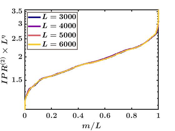
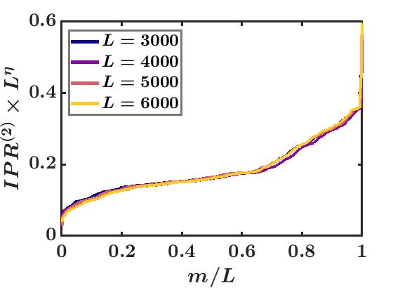
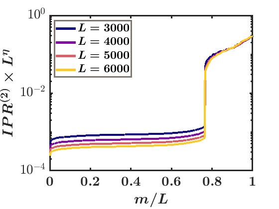
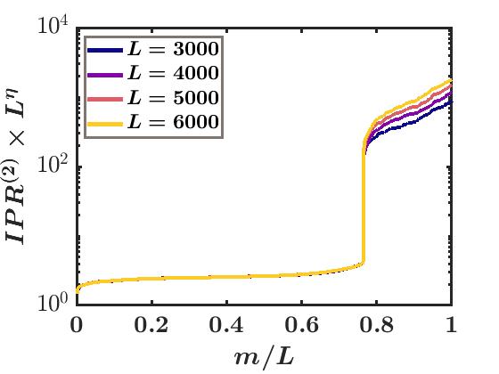
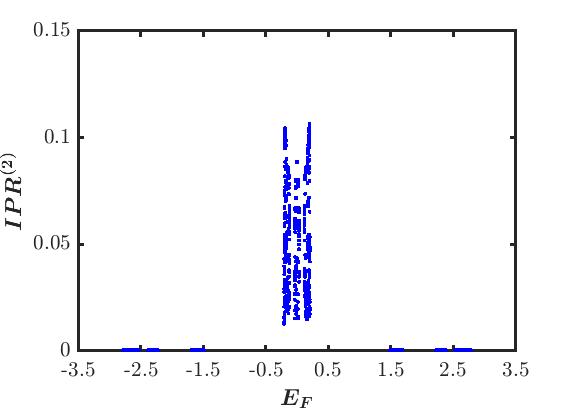
Figure 1: (a-d) Plots of $I_{m}^{(2)}L^{\eta}$ (sorted in increasing order) versus $m/L$ for $\gamma_{1}=1$, $\gamma_{2}=-1$, $V_{0}=2.5$, system sizes $L=3000,~{}4000,~{}5000$ and 6000, and sinusoidal driving. (a) $I_{m}^{(2)}L^{\eta}$ for Floquet eigenstates with $\omega=5$ and $a=5$. The exponent $\eta=1$, and we see that all states are extended. (b) $I_{m}^{(2)}L^{\eta}$ with $\omega=40$ and $a=5$. Here $\eta=0$ showing that all states are localized. (c) and (d) $I_{m}^{(2)}L^{\eta}$ with $\omega=15.1$ and $a=5$. Plots (c) and (d) correspond to $\eta=0$ and 1 respectively, and they clearly show a jump in the IPR value around $m/L\simeq 0.76$. (e) Plot of $I_{m}^{(2)}$ versus quasienergy $E_{F}$ for $\omega=15$, $a=5$, and $L=3000$. We see several gaps in $E_{F}$.

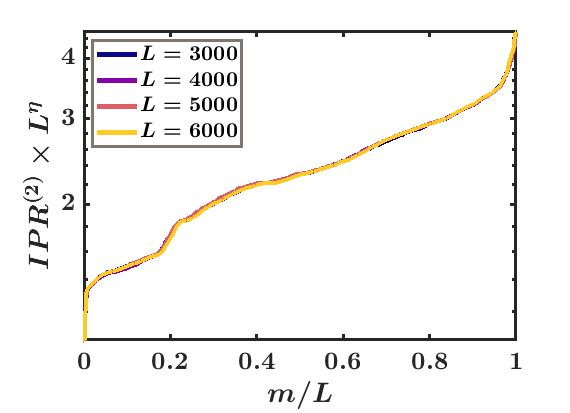
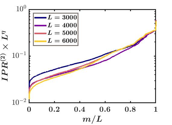
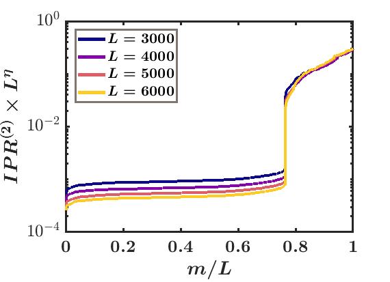
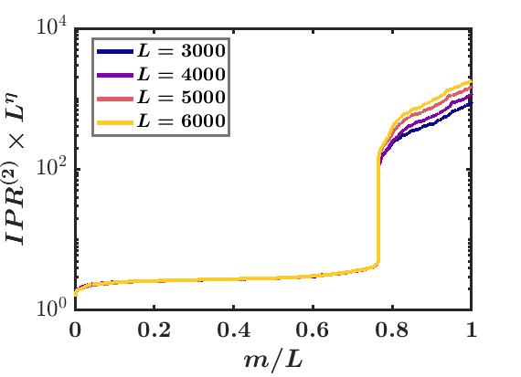
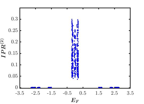
Figure 2: (a-d) Plots of $I_{m}^{(2)}L^{\eta}$ versus $m/L$ and (e) plot of $I_{m}^{(2)}$ versus $E_{F}$ for the same parameter values as in Fig. 1 but obtained using first-order FPT. All the plots agree qualitatively with the plots from exact numerics shown in Fig. 1.

The results obtained using FPT will be compared with those obtained from an exact numerical calculation of the Floquet operator. To this end, we divide the time period $T$ into $N$ steps so that $H(t)$ does not vary appreciably within the time step $\delta t=T/N$. For the present case, we find that $N\sim 500$ achieves this task; a further increase in $N$ does not change the numerical results appreciably. This allows us to use the standard Suzuki-Trotter decomposition to write $U$ as

$$U(T,0) = \prod_{j=1,N}U(t_{j},t_{j-1}),$$

$$U_{j}\equiv U(t_{j},t_{j-1}) = e^{-iH[(t_{j}+t_{j-1})/2]\delta t},$$ (31)

where $t_{0}=0$ and $t_{N}=T$. We can then numerically diagonalize $U$ to obtain its eigenvectors $|\psi_{m}\rangle$ and eigenvalues $e^{-i\theta_{m}}$. We can then write

$$U(T,0)~{}=~{}\sum_{m}e^{-i\theta_{m}}|\psi_{m}\rangle\langle\psi_{m}|.$$ (32)

In this section, we will study and compare the properties of the Floquet eigenstates obtained using first-order FPT and exact numerics. To this end, we compute the inverse participation ratio (IPR) of these eigenstates given, for a normalized Floquet eigenstate $m$, as

$$I_{m}^{(2)}~{}=~{}\sum_{j=1}^{L}|\psi_{m}(j)|^{4}.$$ (33)

It is well-known that $I_{m}^{(2)}$ can distinguish between localized and extended states; $I_{m}^{(2)}\sim L^{-\eta}$ where $\eta=0~{}(1)$ for localized (extended) eigenstates.

III.1 Localized, extended and multifractal states

We now present our numerical results. Figures 1 (a-d) show plots of $I_{m}^{(2)}L^{\eta}$ (sorted in increasing order) versus $m/L$ for systems with $\gamma_{1}=1$, $\gamma_{2}=-1$, $V_{0}=2.5$, different values of $\omega$ and $a$, and sinusoidal driving. For generating this and all subsequent figures, the quasiperiodic potential at site $j$ is taken to be $V_{j}=V_{0}\cos(2\pi\alpha j)$, where $\alpha$ is taken to be a rational approximant for $(\sqrt{5}-1)/2$ by choosing $\alpha=N/L$, where $L$ is the system size, and $N$ is the integer closest to $L(\sqrt{5}-1)/2$. We have chosen $L=3000,~{}4000,~{}5000$ and 6000. The plots clearly indicate a jump in the IPR value for certain ranges of values of $\omega$ and $a$. From Figs. 1 (a) and (b), we find that at relatively low (high) driving frequencies, all the Floquet eigenstates are extended (localized). This can be seen from the collapse of the $I_{m}^{(2)}L^{\eta}$ curves for $\eta=1$ at $\omega=5$ (Fig. 1 (a)) and $\eta=0$ at $\omega=40$ (Fig. 1 (b)) for different $L$. In contrast, at an intermediate driving frequency, $\omega=15.1$, as shown in Figs. 1 (c) and (d), a jump in the IPR between localized and extended eigenstates around $m/L\simeq 0.76$. The data for different $L$ collapses upon scaling with $L^{\eta}$ for two different values of $\eta$; the collapse happens for $\eta=0$ for $m/L\gtrsim 0.764$ (Fig. 1 (c)) and for $\eta=1$ for $m/L\lesssim 0.764$ (Fig. 1 (d)). This demonstrates the appearance of an IPR jump around $m/L\simeq 0.76$ at this driving frequency. Figure 1 (e) shows a plot of $I_{m}^{(2)}$ versus the quasienergy $E_{F}$ for $\omega=5$, $a=5$, and $L=3000$. This clearly shows that there are gaps in the quasienergy spectrum; we call these mobility gaps. (In this paper, we use the term mobility gap regardless of whether the states in the quasienergy bands on the two sides of a gap are both extended or both localized or one extended and the other localized). The states with $E_{F}$ around zero have large IPRs and correspond to localized states, whereas states with $E_{F}$ away from zero (on either the positive or the negative side) have very small IPRs and are extended states. [It is important to note that sorting in increasing order of $I_{m}^{(2)}$ (as done in Figs. 1 (a-d)) and in increasing order of $E_{F}$ (as done in Fig. 1 (e)) are quite different from each other. The presence of mobility gaps becomes apparent only in the latter way of sorting].

In Fig. 2, similar plots are shown for Floquet eigenstates obtained from first-order FPT. These correspond to the same parameter values as their counterparts in Fig. 1. A comparison between Figs. 1 and 2 shows that first-order FPT provides a reasonable match to the exact numerics, although the IPR values found from exact numerics are significantly smaller than the ones found from first-order FPT. Importantly, both exact numerics (Fig. 1 (e)) and first-order FPT (Fig. 2 (e)) show mobility gaps at intermediate driving frequencies like $\omega=5$. We conclude that first-order FPT can provide a good understanding of the driven system when $a\gg\gamma_{1},\gamma_{2}$.

To determine if any of the eigenstates exhibit multifractal behavior, we calculate a generalized IPR defined as

$$I_{m}^{(q)}~{}=~{}\sum_{j}~{}|\psi_{m}(j)|^{2q},$$ (34)

and study its scaling with the system size $L$. sarkar1 ; caste ; evers ; rodri If $I_{m}^{(q)}$ scales as $L^{-\eta_{q}}$ and $\eta_{q}=(q-1)D_{q}$, then $D_{q}=1$ for all $q$ for extended states (since $|\psi_{m}(j)|^{2}$ is of the order of $1/L$ for all $j$ for such states), and $D_{q}=0$ for all $q$ for localized states (since $|\psi_{m}(j)|^{2}$ for such states is of order 1 over a finite region whose size remains constant as $L\to\infty$). Multifractal states typically have $0<D_{q}<1$ for all $q$. Figure 3 shows plots of $I_{m}^{(q)}L^{\eta}$ for $q=3$ and 4 for systems with $\gamma_{1}=1$, $\gamma_{2}=-1$, $\omega=15.1$, $a=5$, $V_{0}=2.5$, different system sizes, and sinusoidal driving. Figures 3 (a) and (c) show that states with $m/L\gtrsim 0.764$ scale with $L$ with the powers $\eta_{3}=\eta_{4}=0$, showing that $D_{q}=0$; hence these states are localized. Figures 3 (b) and (d) show that states with $m/L\lesssim 0.764$ scale with powers $\eta_{3}=2$ and $\eta_{4}=3$, showing that $D_{q}=1$; hence these states are extended. Thus there is no evidence of multifractal states for this set of parameter values. However, we will show below that multifractal behavior appears for a different range of values of $\omega$.

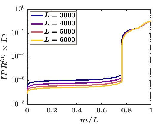
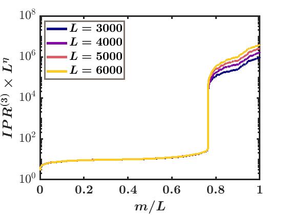
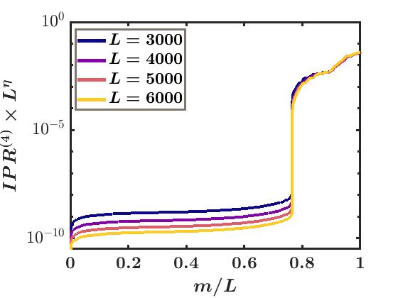
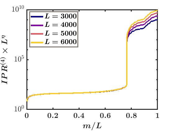
Figure 3: Plots showing $I_{m}^{(3)}L^{\eta}$ and $I_{m}^{(4)}L^{\eta}$ (sorted in increasing order) versus $m/L$ obtained by exact numerical calculations for $L=3000,~{}4000,~{}5000$ and 6000, with $\gamma_{1}=1,~{}\gamma_{2}=-1,~{}a=5,~{}\omega=15.1$, $V_{0}=2.5$, and sinusoidal driving. Plot (a) shows a data collapse of $I_{m}^{(3)}$ with $\eta=0$ for $m/L\gtrsim 0.764$. Plot (b) shows a data collapse of $I_{m}^{(3)}$ with $\eta=2$ for $m/L\lesssim 0.764$. Plot (c) shows a data collapse of $I_{m}^{(4)}$ with $\eta=0$ for $m/L\gtrsim 0.764$. Plot (d) shows a data collapse of $I_{m}^{(4)}$ with $\eta=3$ for $m/L\lesssim 0.764$. These plots show that $I_{m}^{(q)}$ scales with $\eta=0$ for states with $m/L\gtrsim 0.764$ (localized states) and with $\eta=q-1$ for states with $m/L\lesssim 0.764$ (extended states).

In Fig. 4, we show plots of $I_{m}^{(2)}$ and $I_{m}^{(3)}$ versus $m/L$, and their scaling exponents with $L$, $\eta_{2}$ and $\eta_{3}$, versus $\omega$ and $m/L$ for systems with $\gamma_{1}=1$, $\gamma_{2}=-1$, $a=5$, $V_{0}=2.5$, and square pulse driving. Figures 4 (a-b) show $I_{m}^{(2)}$ and $I_{m}^{(3)}$ for a system with $L=3000$, while Figs. 4 (c-d) show the scaling exponents $\eta_{2}$ and $\eta_{3}$ for these two quantities extracted from the results for $L=3000,~{}4000,~{}5000$ and 6000. We see that most states have $\eta_{2}=\eta_{3}=0$ (localized) at lower frequencies and have $\eta_{2}=1$ and $\eta_{3}=2$ (extended) at higher frequencies. Interestingly, however, we see some states for which $\eta_{2}$ and $\eta_{3}$ are different from the values of both localized and extended states. Hence these states have a multifractal nature. In Fig. 4 (e) we show $I_{m}^{(2)}$ versus the quasienergy $E_{Fm}$ for $\omega=30$. For this value of $\omega$, all three kinds of states coexist, extended, multifractal and localized, as is evident from the scaling exponents $\eta_{2}$ and $\eta_{3}$ shown in Figs. 4 (c-d). We have also studied what happens if the driving is sinusoidal instead of square pulse and we find similar results which we do not show here. This demonstrates that the generation of multifractal states does not depend significantly on the driving protocol.

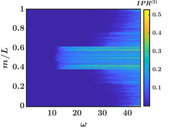
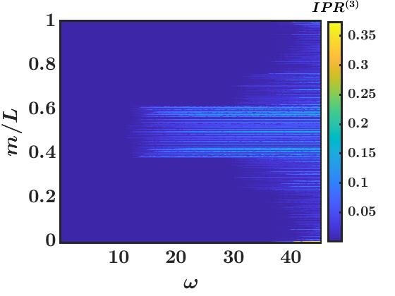
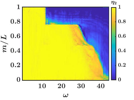
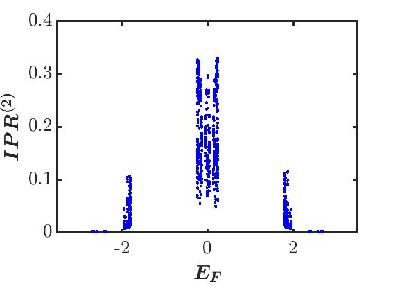
Figure 4: (a-b) Plots of $I_{m}^{(2)}$ and $I_{m}^{(3)}$ (sorted in increasing order of quasienergy $E_{Fm}$) versus $\omega$ and $m/L$ for $\gamma_{1}=1$, $\gamma_{2}=-1$, $a=5$, $V_{0}=2.5$, $L=3000$, and square pulse driving. (c-d) Plots of $\eta_{2}$ and $\eta_{3}$ (extracted from the IPRs sorted in increasing order for $L=3000,~{}4000,~{}5000$ and 6000) versus $\omega$ and $m/L$, with the parameter values same as in plots (a-b). Multiple jumps in $I_{m}^{(2)}$ and $I_{m}^{(3)}$ observed in plots (a-b) indicate multiple localization-delocalization transitions. This is more evident in plots (c-d) where $\eta_{2}$ and $\eta_{3}$ are extracted from the scaling analysis of IPR values. We note that for $30\lesssim\omega\lesssim 45$ in plots (c-d), the values of $\eta_{2}$ and $\eta_{3}$ for a small fraction of states are different from the usual scaling exponents of both extended states ($\eta_{2}=1$ and $\eta_{3}=2$) and localized states ($\eta_{2}=\eta_{3}=0$). Plot (e) shows $I_{m}^{(2)}$ as a function of $E_{Fm}$ (sorted in increasing order) for $\gamma_{1}=1$, $\gamma_{2}=-1$, $a=5$, $V_{0}=2.5$, $\omega=30$ and $L=3000$.

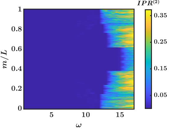
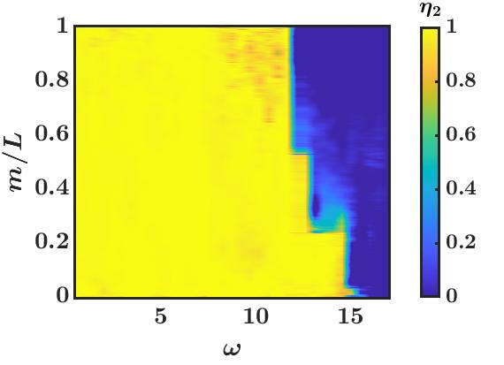
Figure 5: (a) Plot of $I_{m}^{(2)}$ (sorted in increasing order of quasienergy) versus $\omega$ and $m/L$ with $\gamma_{1}=\gamma_{2}=1$ (uniform hopping), $a=5$, $V_{0}=2.5$, $L=3000$, and square pulse driving. (b) Plot of $\eta_{2}$ (extracted from the IPRs sorted in increasing order for $L=3000,~{}4000,~{}5000$ and 6000) versus $\omega$ and $m/L$.

Figure 5 shows plots of $I_{m}^{(2)}$ and the scaling exponent $\eta_{2}$ versus $\omega$ and $m/L$ for $L=3000,~{}4000,~{}5000$ and 6000, for $\gamma_{1}=\gamma_{2}=1$ (uniform hopping), $a=5$, $V_{0}=2.5$, and square pulse driving. The results looks somewhat similar to those shown in Fig. 4 for $\gamma_{1}=-\gamma_{2}=1$ (staggered hopping) in that both extended and localized states appear in the two cases. However, extended states persist up to a larger values of $\omega$ for $\gamma_{1}=-\gamma_{2}=1$ compared to $\gamma_{1}=\gamma_{2}=1$.

It is useful to look at the average values of both $I_{m}^{(2)}$ and the normalized participation ratio (NPR) which, up to a factor of $L$, is the inverse of $I_{m}^{(2)}$. li For the $m$-th Floquet eigenstate, the NPR is defined as ${\rm NPR}_{m}=1/(LI_{m}^{(2)})$. The average values of these two quantities are then defined as $\langle{\rm IPR}\rangle=(1/L)\sum_{m}I_{m}^{(2)}$ and $\langle{\rm NPR}\rangle=(1/L)\sum_{m}{\rm NPR}_{m}$. For a large system size $L$, we have $I_{m}^{(2)}\sim 1/L~{}(1)$ and ${\rm NPR}_{m}\sim 1~{}(1/L)$ for an extended (localized) state $m$, respectively. Hence, the quantity $\phi=\log_{10}(\langle{\rm IPR}\rangle\langle{\rm NPR}\rangle)$ will be large and negative (of the order of $-\log_{10}L$) either if all states are extended or if all states are localized. But if $\phi$ is not large and negative, this would indicate that there are some states which are neither extended nor localized. We will also look at the average value of the Shannon entropy as another measure of the degree of localization dynloc4 . For the $m$-th Floquet eigenstate, the Shannon entropy is defined as $S_{m}=-\sum_{n}|\psi_{m}(n)|^{2}\ln(|\psi_{m}(n)|^{2})$, and its average is then given by $\langle S\rangle=(1/L)\sum_{m}S_{m}$). For an extended (localized) state $m$, we have $S_{m}\sim\ln L~{}(0)$, respectively. Hence the average value $\langle S\rangle$ will be of order $\ln L$ if all states are extended and will be close to zero if all states are localized.

Figure 6 shows plots of $\langle{\rm IPR}\rangle$, $\phi=\log_{10}(\langle{\rm IPR}\rangle\langle{\rm IPR}\rangle$), and $\langle S\rangle$ versus $\omega$ and $V_{0}$, for a system with $\gamma_{1}=1$, $\gamma_{2}=-1$, $a=5$ and square pulse driving. Figure 6 (a) indicates that all states are extended when both $\omega$ and $V_{0}$ are small and are localized when both $\omega$ and $V_{0}$ are large. For $2\lesssim V_{0}\lesssim 3.5$, we see that only extended states low values of $\omega$, coexisting states of different types for intermediate values of $\omega$, and only localized states for large values of $\omega$. Interestingly, when $V_{0}\gtrsim 3.5$, we find multiple re-entrant transitions between regions with only extended and only localized states as $\omega$ is increased. These observations are confirmed qualitatively by Figs. 6 (b) and (c). We note that the range of values of $V_{0}$ which supports re-entrant transitions is the same range where the time-independent part of the model exhibits only localized states.

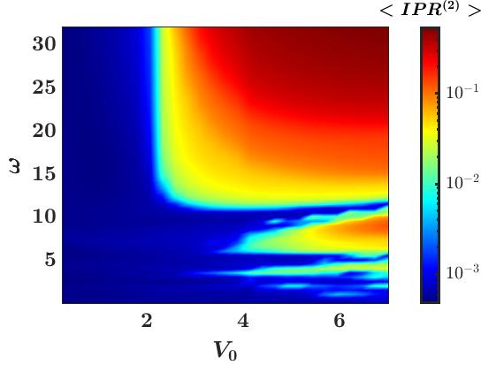
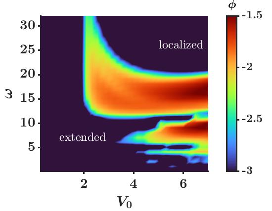
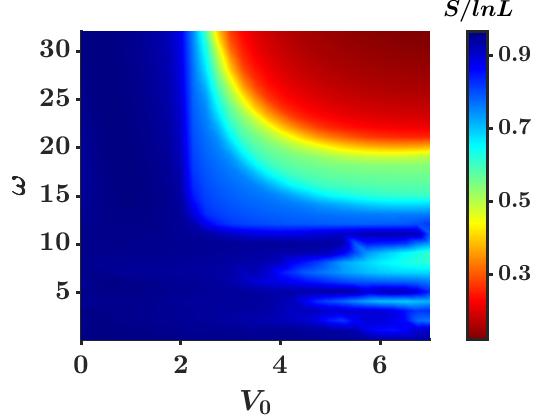
Figure 6: (a) Plot on a log scale of the average of $I_{m}^{(2)}$, denoted as $\langle IPR\rangle$, versus $V_{0}$ and $\omega$ for $\gamma_{1}=1,\gamma_{2}=-1$, $a=5$, $L=3000$, and square pulse driving. (b) Plot of $\phi=\log_{10}({\langle\text{IPR}\rangle\langle\text{NPR}\rangle})$ versus $V_{0}$ and $\omega$. (c) Plot of the average Shannon entropy $\langle S\rangle$ versus $V_{0}$ and $\omega$. Plots (a-c) suggest that all the Floquet eigenstates below $V_{0}\simeq 2$ are extended for all values of $\omega$. For $2\lesssim V_{0}\lesssim 3.5$, we find three distinct regions, with only extended states for small $\omega$, coexisting states of different types for intermediate $\omega$, and only localized states for large $\omega$. A different behavior appears for $V_{0}\gtrsim 3.5$, where we see multiple re-entrant transitions between regions with only extended and only localized states as $\omega$ is increased.

Figure 7 shows plots of $I_{m}^{(2)}$, the scaling exponent $\eta_{2}$ and the real part of the Floquet eigenvalues versus $\omega$ and $m/L$ for systems with $\gamma_{1}=1$, $\gamma_{2}=-1$, $a=5$, $V_{0}=5.5$ and different sizes, for square pulse driving. This figure confirms the multiple re-entrant transitions between regions which are completely extended, completely localized, or have both extended and localized states, that we see in Fig. 6 when $V_{0}\gtrsim 3.5$. (We note that similar re-entrant transitions have been observed in a kicked quasicrystal grover ). We would like to mention here that the plots in Fig. 7 are difficult to explain by any perturbation theory since the values of $a$, $\omega$ and $V_{0}$ are all comparable to each other.

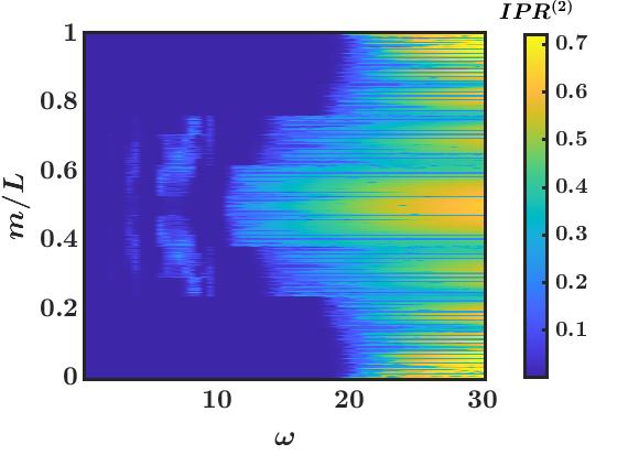
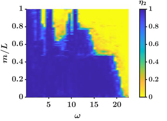
Figure 7: (a) Plot of $I_{m}^{(2)}$ (sorted in increasing order of quasienergy) versus $\omega$ and $m/L$, with $\gamma_{1}=1$, $\gamma_{2}=-1$, $a=5$, $V_{0}=5.5$, $L=3000$, and square pulse driving. (b) Plot of $\eta_{2}$ versus $\omega$ and $m/L$. We extract $\eta_{2}$ using system sizes $L=3000,~{}4000,~{}5000$ and 6000. The plots confirm the multiple transitions seen in Fig. 6 for $V_{0}\gtrsim 3.5$ as $\omega$ is varied. Plot (b) shows several transitions. A transition to a phase with all extended states occurs at $\omega\simeq 5.1$, and this phase then continues up to $\omega\simeq 7.1$. For $\omega\gtrsim 7.1$, we get both extended and localized states till $\omega\simeq 9.1$. Another phase of extended states appears for $9.2\lesssim\omega\lesssim 12.1$. Beyond $\omega\simeq 12.1$, plot (b) suggests that the system moves towards complete localization as $\omega$ increases.

Fig. 8 shows the average $\langle{\rm IPR}\rangle$ and average Shannon entropy $\langle S\rangle$ as functions of $V_{0}$ and of $\omega$ for a system with uniform hopping, $\gamma_{1}=\gamma_{2}=1$, $a=5$ and $L=3000$, for square pulse driving. The results deviate significantly from the case of staggered hopping, $\gamma_{2}=-\gamma_{1}$, shown in Fig. 6, particularly for $V_{0}\gtrsim 3.5$.

It is known that there are no re-entrant transitions in the Aubry-André model (which is the time-independent part of our model) if there is no driving. Furthermore, there are no such transitions in a driven model with no quasiperiodic potential. Comparing Fig. 6 (where $\gamma_{2}=-\gamma_{1}$) and Fig. 8 (where $\gamma_{2}=\gamma_{1}$), we see that staggered hopping, driving and quasiperiodic potential are all necessary to clearly see re-entrant transitions between delocalized states and other kinds of states.

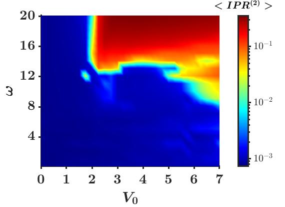
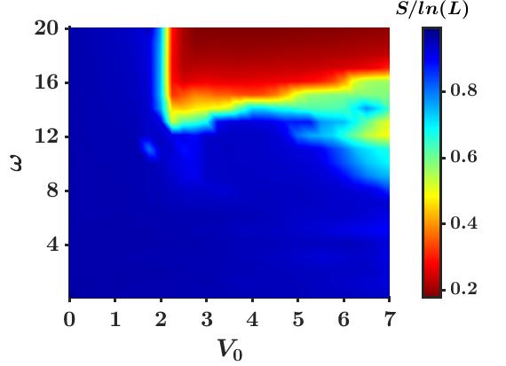
Figure 8: (a) Plot on a log scale of the average of $I_{m}^{(2)}$, $\langle{\rm IPR}\rangle$, versus $\omega$ and $V_{0}$, with $\gamma_{1}=\gamma_{2}=1$ (uniform hopping), $a=5$, $L=3000$, and square pulse driving. (b) Plot of average Shannon entropy, $\langle S\rangle$, versus $\omega$ and $V_{0}$. For $V_{0}\gtrsim 3.5$, we see that the case of uniform hopping shown here deviates significantly from the case of non-uniform hopping shown in Fig. 6.

III.2 High-frequency limit

In the high-frequency limit $\omega\gg a\gg\gamma_{1},~{}\gamma_{2},~{}V_{0}$, we expect the effects of driving to disappear as we have argued in Sec. II Surprisingly, however, we find that although the quasienergies for large $\omega$ match the energies for the undriven system, the IPRs do not agree in the two cases.

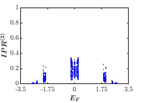
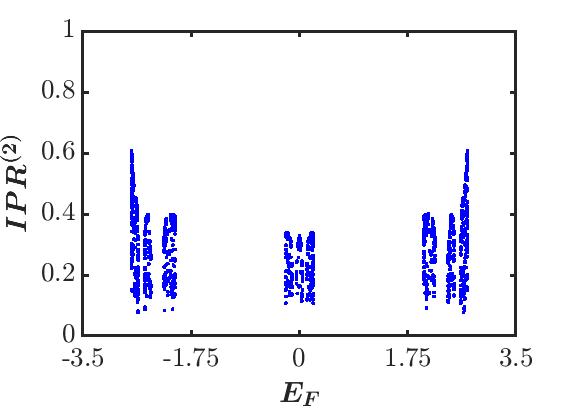
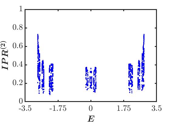
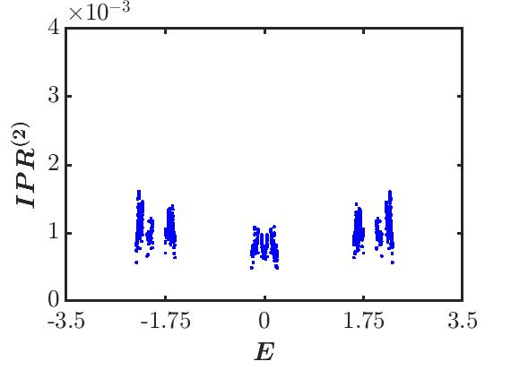
Figure 9: (a) Plot of $I_{m}^{(2)}$ versus quasienergy $E_{F}$ (sorted in increasing order) for a system with $\gamma_{1}=1$, $\gamma_{2}=-1$, $\omega=35$, $a=5$, $V_{0}=2.5$, $L=3000$, and square pulse driving. (b) Plot of $I_{m}^{(2)}$ versus quasienergy for a system with $\gamma_{1}=1$, $\gamma_{2}=1$ (uniform hopping), $\omega=35$, $a=5$, and $V_{0}=2.5$. (c) Plot of $I_{m}^{(2)}$ versus energy $E$ (sorted in increasing order) for an undriven system ($a=0$) with $\gamma_{1}=1$, $\gamma_{2}=1$, and $V_{0}=2.5$. (d) Plot of $I_{m}^{(2)}$ versus energy $E$ (sorted in increasing order) for an undriven system ($a=0$) with $\gamma_{1}=1$, $\gamma_{2}=-1$, and $V_{0}=1.5$. Note that the range of IPR values in plot (d) is much smaller than in plots (a-c). In all cases we have considered system size $L=3000$ and square pulse driving.

In Figs. 9 (a) and (b), we show plots of $I_{m}^{(2)}$ versus quasienergy $E_{F}$ (sorted in increasing order) for systems with $\gamma_{1}=1$, $\gamma_{2}=-1$ and $+1$ respectively, $\omega=35$, $a=5$, $V_{0}=2.5$, $L=3000$, and square pulse driving. Fig. 9 (c) shows a plot of $I_{m}^{(2)}$ versus energy $E$ (sorted in increasing order) for an undriven system with $\gamma_{1}=1$, $\gamma_{2}=1$ (the relative sign of $\gamma_{1}$ and $\gamma_{2}$ is unimportant in the absence of driving), $V_{0}=2.5$, and $L=3000$. We have chosen $V_{0}=2.5$ so that $V_{0}>2\gamma_{1}$ and all the states of the undriven system are localized. We note that the quasienergies in plots (a) and (b) and the energies in plot (c) have almost the same values. This is expected since driving at high frequencies should give the same Floquet Hamiltonian as the undriven part of the Hamiltonian. Surprisingly, however, the IPR values are not the same in the three plots. The IPR values for the driven system with uniform hopping amplitudes differ only a little from the IPRs of the undriven system, but the IPRs of the driven staggered model ($\gamma_{2}=-\gamma_{1}$) differ substantially from those of the undriven system. (This may be because driving has a smaller effect when $\gamma_{2}=\gamma_{1}$ compared to $\gamma_{2}=-\gamma_{1}$, for reasons explained after Eq. (22)). We observe that the undriven system (plot (c)) shows only localized states, but the driven staggered model (plot (a)) shows that some of the states have very low IPR values and are therefore extended states. Thus driving even at a high frequency seems to convert some of the localized states to extended states, provided that $a\gg\gamma_{1},~{}\gamma_{2}$ and $V_{0}$. (We have checked numerically that if $a\ll\gamma_{1},~{}\gamma_{2}$ and $V_{0}$, then all the states remain localized). This suggests that although terms of order $1/\omega$ and higher in the Floquet Hamiltonian are small for large $\omega$, they have a significant effect on the IPR values of the Floquet eigenstates. It is possible that these small terms have a negligible effect on the quasienergies, but they couple localized states which lie close to each other and this hybridization produces extended states.

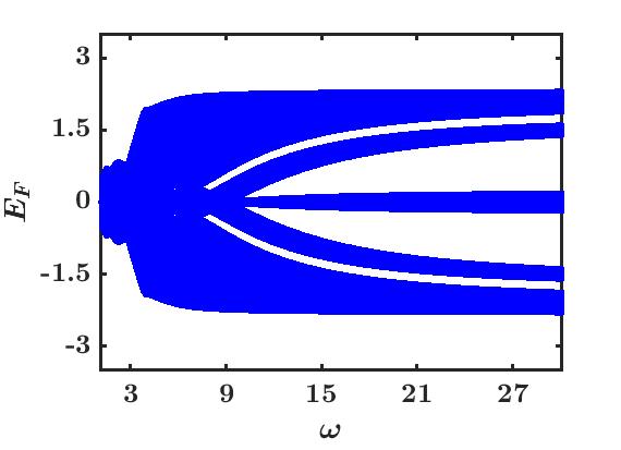
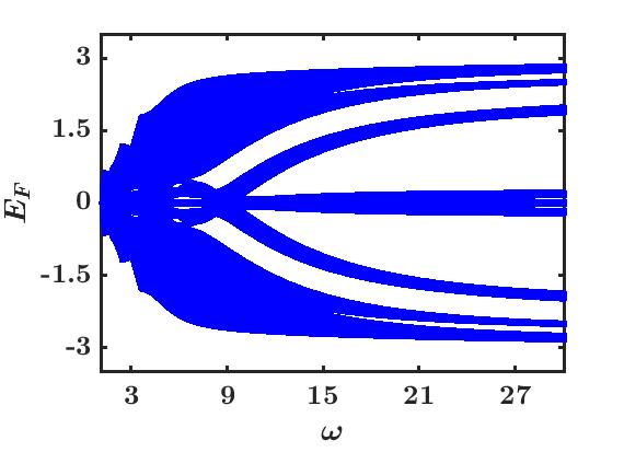
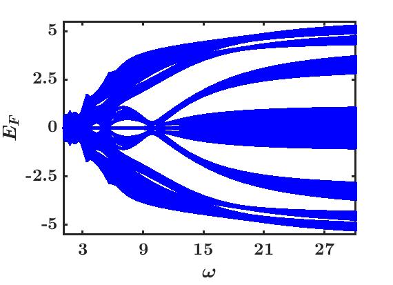
Figure 10: Plots of $E_{Fm}$ versus for $\omega$ for (a) $V_{0}=1.5$, (b) $V_{0}=2.5$, and (c) $V_{0}=5.5$, for systems with $\gamma_{1}=1$, $\gamma_{2}=-1$, $a=5$, size $L=2000$, and square pulse driving. The spectrum of $E_{Fm}$ is gapless for intermediate $\omega$ and develops several gaps as $\omega$ increases.

On the other hand, if we choose $V_{0}<2\gamma_{1}$ and all the other parameters are the same as in Figs. 9 (a-c), we find that there is no discernible differences between the spectra of quasienergies (or energies) and IPR values in the three cases. All the states are extended in all three cases (driven with $\gamma_{2}=\pm\gamma_{1}$ and undriven). Fig. 9 (d) shows a plot of the energies and corresponding IPR values for an undriven system with $\gamma_{1}=1$, $\gamma_{2}=-1$, and $V_{0}=1.5$. The IPR versus quasienergy plots for the driven systems with $\gamma_{2}=\pm\gamma_{1}$ look the same and are not shown here.

In Fig. 10, we show plots of all the quasienergies $E_{Fm}$ for systems with $\gamma_{1}=1$, $\gamma_{2}=-1$, $a=5$, size $L=2000$, square pulse driving, and (a) $V_{0}=1.5$, (b) $V_{0}=2.5$, and (c) $V_{0}=5.5$. We have chosen these three values of $V_{0}$ for the following reason. For $V_{0}=1.5$, all states are found to be extended. For $V_{0}=2.5$, various kinds of states can coexist depending on the values of $\omega$, as we see in Fig. 4. For $V-0=5.5$, we find re-entrant transitions as shown in Fig. 7. The plots in Fig. 10 show that the spectrum of $E_{Fm}$ is generally gapless for intermediate frequencies but several gaps appear as $\omega$ is increased. This can be qualitatively understood from the FPT as follows. In the limit that $\gamma_{1},~{}\gamma_{2},~{}V_{0}\ll\omega\ll a$, we saw in the discussion given towards the end of Sec. II that the model reduces to one in which the hopping amplitude is uniform and the quasiperiodic potential is absent. This system clearly has no gaps in the spectrum. On the other hand, when $\gamma_{1},~{}\gamma_{2},~{}V_{0}\ll a\ll\omega$, we saw that the model reduces to an undriven system ($a=0$). Hence the quasienergies will approach the energies of the undriven system. For the undriven Aubry-André model, it is known that there is a large number (in fact, an infinite number) of energy gaps for any non-zero value of $V_{0}$. aubry ; soko It would be useful to understand precisely how the different gaps appear successively as $\omega$ is increased from intermediate to large values. [We have checked numerically that for $V_{0}=0$, there are no gaps for any value of $\omega$ or $a$. Hence the gaps seen in Fig. 10 are entirely due to the presence of a quasiperiodic potential].

III.3 Floquet Hamiltonian in real space

To visualize the effects of localization, it is instructive to look at the matrix elements of the Floquet Hamiltonian. Figure 11 shows the absolute values of the matrix elements of $H_{F}(X,Y)$ in real space for systems with $\gamma_{1}=1$, $\gamma_{2}=-1$, $V_{0}=2.5$, size $L=2000$, and sinusoidal driving. $H_{F}(X,Y)$ is obtained by doing a Fourier transform of $H_{F}$ in momentum space as found numerically from the Floquet operator $U$ (Figs. 11 (a-c)). The plots are shown as a function of $Y-X$ and $X$. If the system was translation invariant, the plot would depend only on the relative coordinate $Y-X$ and not on $X$. Indeed we see that the plots do not vary with $X$ at length scales much larger than $1/\beta\simeq 1.62$ (which is the length scale of variation of the quasiperiodic potential $\cos(2\pi\beta j)$). In terms of the relative coordinate $Y-X$, the plots show a large spread in Fig. 11 (a) corresponding to all states being extended, a smaller spread in Fig. 3 (b) corresponding to a case where there are both localized and extended states, and a very small spread in Fig. 11 (c) corresponding to all states being extended. We find that $H_{F}(X,Y)$ obtained by doing a Fourier transform of $H_{F}$ in momentum space as found from the first-order FPT gives very similar results, and we do not show those plots here.

A more detailed explanation of the results shown in Fig. 11 is as follows. We know that although the Hamiltonian of the undriven Aubry-André model is local in real space, it exhibits a delocalized phase below a critical disorder strength. We now look at the structure of matrix elements of the Floquet Hamiltonian $H_{F}(X,Y)$ in real space. In all the plots in Fig. 11, we have taken we consider $\gamma_{1}=1$, $\gamma_{2}=-1$, $a=5$, and $V_{0}=2.5$. $V_{0}=2.5$ necessarily implies that the static model exhibits a localized phase in the absence of driving. However, in the presence of driving and with diminishing values of $\omega$, we observe a significant decrease in the value of the diagonal elements $H_{F}(X,X)$. The values of these elements is found to be about 2 for $\omega$=40, about $1.2$ for $\omega$=15.1, and about $0.35$ for $\omega$=5. The decreasing value of the diagonal elements implies that the effective strength of the quasiperiodic potential is decreasing. Furthermore, we find that there is a rapid spreading of the off-diagonal matrix elements signifying a growing non-locality of $H_{F}$ as $\omega$ decreases. The combination of these two effects leads the system towards increasing delocalization.

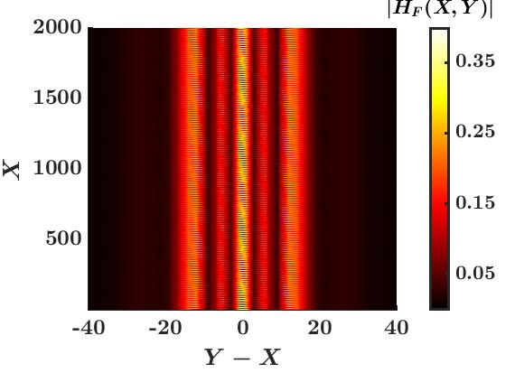
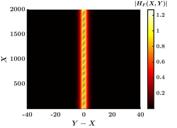
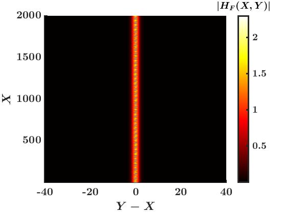
Figure 11: Plots of the absolute values of the matrix elements of the Floquet Hamiltonian $H_{F}(X,Y)$ in real space ($X$ and $Y$ represent space coordinates), where the axes are chosen to be $X$ and $Y-X$. In all cases, we considered $\gamma_{1}=1,~{}\gamma_{2}=-1$, $V_{0}=2.5$, system size $L=2000$, and sinusoidal driving. Figures (a-c) are obtained from exact numerical calculations. The parameters used are (a) $a=10,~{}\omega=5$, (b) $a=5,~{}\omega=15.1$, and (c) $a=5,~{}\omega=40$. We note that plot (a) and (d) is for a system with only extended states, plot (b) is for a system with both extended and localized states, and plot (c) is for a system with only localized states.

III.4 Spreading of a one-particle wave packet

We now consider a measure of delocalization given by the spreading of a one-particles state which is initially localized at the middle site of system of size $L$, namely, the site $j_{0}=L/2$. This initial state, denoted $|\psi_{in}\rangle$, is evolved over $n$ time periods by acting on it with the Floquet operator $n$ times. This gives

$$|\psi_{nT}\rangle~{}=~{}U^{n}~{}|\psi_{in}\rangle.$$ (35)

The root mean squared displacement is then given by

$$\sigma(n)~{}=~{}[\sum_{j}~{}(j-j_{0})^{2}~{}|\psi_{nT}(j)|^{2}]^{1/2}.$$ (36)

The growth of $\sigma(n)$ with $n$ gives an idea of how delocalized the system is. Fig. 12 shows plots of $\sigma(n)$ for systems with $\gamma_{1}=1$, $\gamma_{2}=\pm 1$ (uniform and staggered hopping amplitudes respectively), $a=5$, $\omega=5$ and 30, various values of $V_{0}$, and square pulse driving. (The system size $L$ is taken to be 6000). We see that the spreading of the wave packet is always ballistic. The ballistic velocity, given by the slope of $\sigma(n)$ versus $n$, is smaller for $\omega=30$ compared to $\omega=5$. This is because driving with a very large frequency is equivalent to not driving at all. In the absence of driving, it is known that a system with a quasiperiodic potential with strength $V_{0}<2\gamma_{1}$ has only extended states, while a system with $V_{0}>2\gamma_{1}$ has only localized states aubry ; soko ; these results hold regardless of whether $\gamma_{2}=\gamma_{1}$ or $\gamma_{2}=-\gamma_{1}$ since we can change the sign of $\gamma_{2}$ by doing a unitary transformation which does not affect $\gamma_{1}$ and $V_{0}$. Indeed we see in Figs. 12 (b) and (d), that the wave packet spreads ballistically if $V_{0}<2$ but remains completely localized if $V_{0}>2$. The situation at the lower frequency, $\omega=5$, is more interesting. The system with staggered hopping, $\gamma_{2}=-\gamma_{1}$, shows ballistic spreading for $V_{0}=1.5,~{}3$ and 6, and no spreading for $V_{0}=9$. However, the system with uniform hopping, $\gamma_{2}=\gamma_{1}$, always shows some ballistic spreading for all values of $V_{0}$. Furthermore, the ballistic velocity is a non-monotonic function of $V_{0}$, being smaller for $V_{0}=1.5$ and 9 compared to $V_{0}=3$ and 6. A similar non-monotonic behavior of the ballistic spreading is seen in Fig. 13 for driving at an intermediate frequency with $\omega=12$.

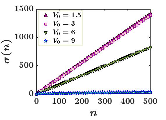
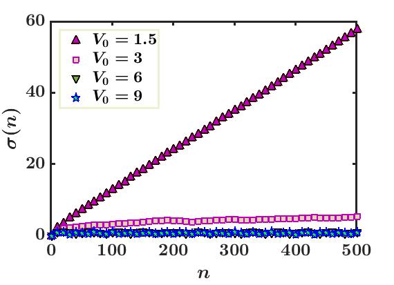
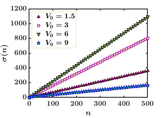
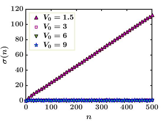
Figure 12: (a-b) Root mean squared displacement, $\sigma(n)$, versus the stroboscopic evolution number $n$ for $\gamma_{1}=1$, $\gamma_{2}=-1$, $a=5$, and $\omega=5$ and $\omega=30$ respectively, for a one-particle state which is initially located at the middle site of a large system. (c-d) Plot of $\sigma(n)$ versus $n$ for $\gamma_{1}=\gamma_{2}=1$ (uniform hopping), $a=5$, and $\omega=5$ and $\omega=30$, respectively. All the figures are for system size $L=6000$ and square pulse driving. Plots (a-b) show that compared to the high-frequency regime (where the behavior is similar to an undriven system), the intermediate-frequency regime shows a ballistic behavior up to a larger value of $V_{0}$ for the case of staggered hopping compared to uniform hopping. For the uniform hopping system at the lower value of $\omega=5$, plot (c) exhibits a non-monotonic ballistic velocity of $\sigma(n)$ as a function of $V_{0}$ before showing a completely localized behavior for large $V_{0}$. Such a non-monotonic behavior is not seen at the higher value of $\omega=30$ as shown in plot (d).

IV Perturbation theory for a model with uniform hopping

In this section we will study a system with a uniform hopping amplitude, $\gamma_{1}=\gamma_{2}=1$, which is driven by a square pulse. For uniform hopping, the unit cell consists of a single site and we will denote the fermionic operator as $c_{j}$. The Hamiltonian is given by

$$H(t) = (1+f(t))\sum_{j}~{}(c_{j}^{\dagger}c_{j+1}+{\rm H.c.})$$ (37)

$$+~{}V_{0}~{}\sum_{j}\cos(2\pi\beta j)~{}c_{j}^{\dagger}c_{j},$$

where $f(t)$ has the square pulse form described in Eq. (26). Note that for $V_{0}=0$, the periodic driving would have no effect since the time-independent and driven parts of the Hamiltonian commute with each other in that case, and the Floquet Hamiltonian $H_{F}$ would just be given by $\sum_{j}(c_{j}^{\dagger}c_{j+1}+{\rm H.c.})$ independently of the driving frequency.

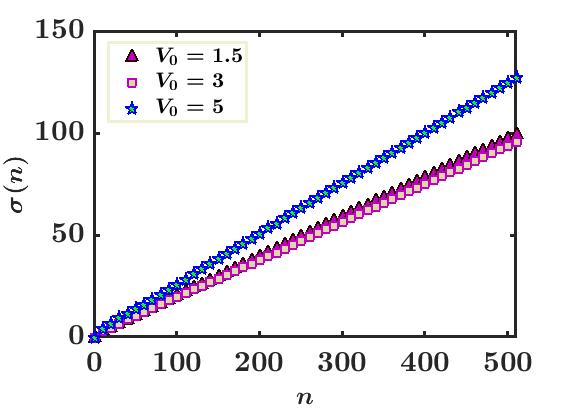
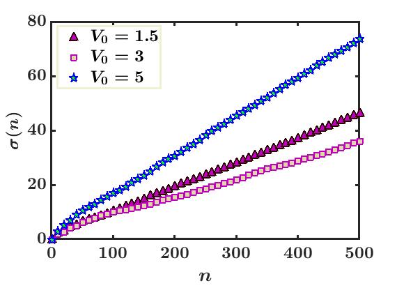
Figure 13: (a) Root mean squared displacement, $\sigma(n)$, versus the stroboscopic evolution number $n$ from the exact numerical calculation with $\gamma_{1}=\gamma_{2}=1$ (uniform hopping), $a=5$, and $\omega=12$. (b) $\sigma(n)$ versus $n$ as obtained from the second-order Floquet Hamiltonian in Sec. IV. Both figures are for $L=3000$ and square pulse driving. The two figures agree qualitatively and indicate a non-monotonic ballistic velocity of $\sigma(n)$ as $V_{0}$ increases.

We will now find the Floquet Hamiltonian $H_{F}$ in the high-frequency regime using van Vleck perturbation theory rev4 ; rev6 . This is a perturbative expansion in powers of $1/\omega$, and it has the advantage over the Floquet-Magnus expansion that it does not depend on the phase of the driving protocol, i.e., it is invariant under $f(t)\to f(t+t_{0})$. Furthermore, unlike the FPT which gives us $H_{F}$ in momentum space, the van Vleck perturbation theory gives us $H_{F}$ in real space. This makes it more suitable for studying the dynamics of a wave packet.

The zeroth-order Floquet Hamiltonian given by van Vleck perturbation theory turns out to be

$$H_{F}^{(0)} = \frac{1}{T}~{}\int_{0}^{T}dt~{}H(t)$$

$$= \sum_{j}(c_{j}^{\dagger}c_{j+1}+{\rm H.c.})+V_{0}\sum_{j}\cos(2\pi\beta j)~{}c_{j}^{\dagger}c_{j}.$$

The $m$-th Fourier component of $H(t)$ is given by

$$H_{m} = \frac{2ia}{m\pi}\sum_{j}(c_{j}^{\dagger}c_{j+1}+{\rm H.c.})~{}~{}{\rm for}~{}~{}m~{}~{}\text{odd},$$ (39)

$$= 0~{}~{}{\rm for}~{}~{}m~{}~{}\text{even ~{}and}~{}\neq 0,$$

and $H_{0}=H_{F}^{(0)}$. We then find that the first-order Floquet Hamiltonian, $H_{F}^{(1)}=\sum_{m\neq 0}\left[H_{-m},H_{m}\right]/(2m\omega)$, is zero since $H_{-m}=(-1)^{m}H_{m}$ for all $m$. The second-order Floquet Hamiltonian consists of two terms

$$H_{F}^{(2)} = \sum_{m\neq 0}\frac{[[H_{-m},H_{0}],H_{m}]}{2m^{2}\omega^{2}}$$ (40)

$$+\sum_{m\neq 0}\sum_{n\neq 0}\frac{[[H_{-m},H_{m-n}],H_{n}]}{3mn\omega^{2}}.$$

The first term in Eq. (40) takes the form

$$H_{F}^{(2)} = 2t_{2}\sum_{j}~{}[\cos(2\pi\beta(j+1))+\cos(2\pi\beta(j-1))$$ (41)

$$~{}~{}~{}~{}~{}~{}~{}~{}~{}~{}~{}~{}~{}~{}-2\cos(2\pi\beta j)]~{}c_{j}^{\dagger}c_{j}$$

$$+t_{2}\sum_{j}~{}[2\cos(2\pi\beta(j+1))-\cos(2\pi\beta(j+2))$$

$$~{}~{}~{}~{}~{}~{}~{}~{}~{}~{}~{}~{}~{}~{}-\cos(2\pi\beta j)]~{}(c_{j}^{\dagger}c_{j+2}+{\rm H.c.}),$$

where $t_{2}=a^{2}T^{2}V_{0}/96$. The second term in Eq. (40) turns out to be zero. The third-order Floquet Hamiltonian vanishes due to the symmetry given in Eq. (29). In principal we can calculate higher order terms but such corrections are expected to be small compared to $H_{F}^{(0)}$ and $H_{F}^{(2)}$.

Fig. 13 shows a comparison between the results obtained for the root mean squared displacement $\sigma(n)$ versus the stroboscopic evolution number $n$ as obtained from exact numerics and the second-order Floquet Hamiltonian derived above, for systems with $a=5$, $\omega=12$, various values of $V_{0}$, and square pulse driving. We find a qualitative agreement between the two sets of results.

We can now understand better the results for staggered hopping and uniform hopping shown in Figs. 12 and 13. Naively, one should expect that the spreading of the wave function should diminish as the value $V_{0}$ of the quasiperiodic potential increases. However, in the uniform hopping case and in the presence of driving, we observe in Figs. 12 and 13 that the ballistic spreading velocity first increases and then decreases (Fig. 12) and vice versa (Fig. 13) with increasing $V_{0}$ depending on the values of $\omega$. It is difficult to obtain any analytical insight for the first case (Fig. 12) since the parameter values do not allow us to perform a perturbative expansion. The second case (Fig. 13) can, however, be explained using the Floquet van Vleck Hamiltonian described above. The zeroth-order term in this Hamiltonian is just the Aubry-André model as expected. But the second-order term contains a second nearest-neighbor quasiperiodic hopping as well as a quasiperiodic on-site potential. Furthermore, both these terms depend on $V^{2}_{0}/\omega$. We believe that these competing terms in $H_{F}$ can give rise to a non-monotonic dependence of the velocity of spreading as a function of $V_{0}$. To support this statement, we compare the wave packet dynamics obtained from the exact numerical calculation with the one obtained from the van Vleck Hamiltonian in Fig. 13. We observe that the two results qualitatively agree with each other.

V Discussion

We will now summarize our results. We considered a one-dimensional model with time-independent staggered hopping amplitudes $\gamma_{1}$ and $\gamma_{2}$ and a periodically driven uniform hopping amplitude between nearest-neighbor sites, and a quasiperiodic potential with strength $V_{0}$. We have studied the effects of both sinusoidal driving and driving by a periodic square pulse. While we have mainly studied the case of staggered hopping amplitudes, $\gamma_{2}=-\gamma_{1}$, we have also looked at the case with uniform hopping amplitudes, $\gamma_{2}=\gamma_{1}$, for comparison. (In the absence of driving, both these cases reduce to the Aubry-André model, but we find some significant differences between the two cases when they are driven). In the limit that the driving amplitude $a$ and frequency $\omega$ are much larger than $\gamma_{1},~{}\gamma_{2}$ and $V_{0}$, we analytically derived a Floquet Hamiltonian $H_{F}$ to first-order in Floquet perturbation theory. We then numerically computed the Floquet operator $U$. The eigenstates and eigenvalues of $U$ were found, and various properties of the Floquet eigenstates were then examined as follows.

We studied a generalized IPR, called $I_{m}^{(q)}$, of the Floquet eigenstates (labeled as $m$), and found the exponent of their scaling with the system size $L$, namely, $I_{m}^{(q)}\sim 1/L^{\eta_{q}}$. For standard extended states we expect $\eta_{q}=q-1$ for all $q$, while standard localized states have $\eta_{q}=0$ for all $q$. We found that while most states are either extended or localized in a standard way, there are some multifractal states which show an intermediate behavior with $0<\eta_{q}<q-1$ (we have looked at the cases $q=2,~{}3$ and 4). These states typically appear along with re-entrant transitions at intermediate frequencies $\omega$ and large values of $V_{0}$. A study of the average Shannon entropy also suggests that there can be different kinds of states which have very different degrees of localization. In addition, we find re-entrant transitions between regions with extended, localized and multifractal states as $\omega$ is varied. We note that re-entrant transitions have been studied earlier in periodically driven non-Hermitian systems with quasiperiodic potentials longwen .

Interestingly, we find that in the high-frequency limit where $\omega$ is much larger than all the other parameters, $\gamma_{1},~{}\gamma_{2},V_{0}$ and $a$, the quasienergies are almost the same as the energies for the undriven system ($a=0$), but the corresponding IPRs can have quite different values when $V_{0}$ is large and $\gamma_{2}=-\gamma_{1}$. Namely, when $V_{0}$ is larger than the critical value $2\gamma_{1}$, we know that all the states of the undriven system are localized. We then find that periodic driving of this system at a high frequency does not change the spectrum of quasienergies noticeably but significantly reduces some of the IPR values. Thus driving seems to convert some of the localized states to extended states. The exact mechanism by which this happens may be an interesting problem for future studies.

In general, our numerical results show that there are many gaps in the quasienergy which separate states with significantly different values of the IPR (see Figs. 1 (e) and 2 (e) in particular). These mobility gaps appear due to the presence of the quasiperiodic potential. The number of gaps increases as the driving frequency is increased from intermediate to large values, as we see in Fig. 10. It would be useful to study exactly why this happens. Interestingly, our numerical results show only mobility gaps. We have not found any examples of mobility edges which appear when there is a continuous range of quasienergies, and somewhere within that range there is a particular quasienergy which separates localized and extended states.

As a dynamical signature of localization, we have studied how a one-particle state initialized at one particular site of the system evolves in time. For all the parameter values that we have examined, we find that the mean squared displacement always increases linearly in time. The ballistic velocity, given by the slope of the displacement versus time, depends on the system parameters. The velocity generally decreases as either $\omega$ or $V_{0}$ is increased. However, for a system with uniform hopping amplitudes ($\gamma_{2}=\gamma_{1}$) and intermediate values of $\omega$, the velocity shows a non-monotonic dependence on $V_{0}$.

There is some evidence of re-entrant transitions in a recent experiment in which ultracold bosonic atoms are trapped in an optical lattice and the atoms experience a quasiperiodic potential whose strength is given periodic $\delta$-function kicks grover . The experiment finds regimes of parameter space where there are multiple transitions between localized, extended and multifractal states as the strength of the kicked quasiperiodic potential is varied.

Acknowledgments

S.A. thanks MHRD, India for financial support through a PMRF. K.S. thanks DST, India for support through SERB project JCB/2021/000030. D.S. thanks SERB, India for funding through Project No. JBR/2020/000043.

References

- (1)
- (2) S. Blanes, F. Casas, J. A. Oteo, and J. Ros, Physics Reports 470, 151 (2009).
- (3) S. N. Shevchenko, S. Ashhab, and F. Nori, Physics Reports 492, 1 (2010).
- (4) L. D’Alessio and A. Polkovnikov, Ann. Phys. 333, 19 (2013).
- (5) M. Bukov, L. D’Alessio and A. Polkovnikov, Adv. Phys. 64, 139 (2015).
- (6) L. D’Alessio, Y. Kafri, A. Polkovnikov, and M. Rigol, Adv. Phys. 65, 239 (2016).
- (7) T. Mikami, S. Kitamura, K. Yasuda, N. Tsuji, T. Oka, and H. Aoki, Phys. Rev. B 93, 144307 (2016).
- (8) T. Oka and S. Kitamura, Annu. Rev. Condens. Matter Phys. 10, 387 (2019).
- (9) S. Bandyopadhyay, S. Bhattacharjee and D. Sen, J. Phys. Condens. Matter 33, 393001 (2021); A. Sen, D. Sen, and K. Sengupta, J. Phys. Condens. Matter 33, 443003 (2021).
- (10) T. Kitagawa, E. Berg, M. Rudner, and E. Demler, Phys. Rev. B 82, 235114 (2010); T. Kitagawa, T. Oka, A. Brataas, L. Fu, and E. Demler, Phys. Rev. B 84, 235108 (2011).
- (11) N. H. Lindner, G. Refael, and V. Galitski, Nat. Phys. 7, 490 (2011).
- (12) M. Thakurathi, A. A. Patel, D. Sen, and A. Dutta, Phys. Rev. B 88, 155133 (2013); M. Thakurathi, K. Sengupta, and D. Sen, Phys. Rev. B 89, 235434 (2014).
- (13) A. Kundu, H. A. Fertig, and B. Seradjeh, Phys. Rev. Lett. 113, 236803 (2014).
- (14) F. Nathan and M. S. Rudner, New J. Phys. 17, 125014 (2015).
- (15) B. Mukherjee, A. Sen, D. Sen, and K. Sengupta, Phys. Rev. B 94, 155122 (2016); B. Mukherjee, P. Mohan, D. Sen, and K. Sengupta, Phys. Rev. B 97, 205415 (2018).
- (16) V. Khemani, A. Lazarides, R.Moessner, and S. L. Sondhi, Phys. Rev. Lett. 116, 250401 (2016).
- (17) D. V. Else, B. Bauer, and C. Nayak, Phys. Rev. Lett. 117, 090402 (2016).
- (18) J. Zhang, P. W. Hess, A. Kyprianidis, P. Becker, A. Lee, J. Smith, G. Pagano, I.-D. Potirniche, A. C. Potter, A. Vishwanath, N. Y. Yao, and C. Monroe, Nature (London) 543, 217 (2017).
- (19) A. Russomanno, A. Silva, and G. E. Santoro, Phys. Rev. Lett. 109, 257201 (2012).
- (20) A. Lazarides, A. Das, and R. Moessner, Phys. Rev. E 90, 012110 (2014).
- (21) T. Nag, S. Roy, A. Dutta, and D. Sen, Phys. Rev. B 89, 165425 (2014); T. Nag, D. Sen, and A. Dutta, Phys. Rev. A 91, 063607 (2015).
- (22) A. Agarwala, U. Bhattacharya, A. Dutta, and D. Sen, Phys. Rev. B 93, 174301 (2016); A. Agarwala and D. Sen, Phys. Rev. B 95, 014305 (2017).
- (23) D. J. Luitz, Y. Bar Lev, and A. Lazarides, SciPost Phys. 3, 029 (2017); D. J. Luitz, A. Lazarides, and Y. Bar Lev, Phys. Rev. B 97, 020303(R) (2018).
- (24) R. Ghosh, B. Mukherjee, and K. Sengupta, Phys. Rev. B 102, 235114 (2020).
- (25) A. Das, Phys. Rev. B 82, 172402 (2010); S. Bhattacharyya, A. Das, and S. Dasgupta, Phys. Rev. B 86, 054410 (2012); S. S. Hegde, H. Katiyar, T. S. Mahesh, and A. Das, Phys. Rev. B 90, 174407 (2014).
- (26) S. Mondal, D. Pekker, and K. Sengupta, Europhys. Lett. 100, 60007 (2012); U. Divakaran and K. Sengupta, Phys. Rev. B 90, 184303 (2014).
- (27) S. Lubini, L. Chirondojan, G.-L. Oppo, A. Politi, and P. Politi, Phys. Rev. Lett. 122, 084102 (2019).
- (28) M. Heyl, A. Polkovnikov, and S. Kehrein, Phys. Rev. Lett. 110, 135704 (2013).
- (29) A. Sen, S. Nandy, and K. Sengupta, Phys. Rev. B 94, 214301 (2016); S. Nandy, K. Sengupta, and A. Sen, J. Phys. A: Math. Theor. 51, 334002 (2018).
- (30) For a review, see M. Heyl, Rep. Prog. Phys 81, 054001 (2018).
- (31) C. Karrasch and D. Schuricht, Phys. Rev. B 87, 195104 (2013).
- (32) J. N. Kriel and C. Karrasch, and S. Kehrein, Phys. Rev. B 90, 125106 (2014).
- (33) F. Andraschko and J. Sirker, Phys. Rev. B 89, 125120 (2014).
- (34) E. Canovi, P. Werner, and M. Eckstein, Phys. Rev. Lett. 113, 265702 (2014).
- (35) S. Sharma, U. Divakaran, A. Polkovnikov, and A. Dutta, Phys. Rev. B 93, 144306 (2016); S. Bandyopadhyay, A. Polkovnikov, and A. Dutta, Phys. Rev. Lett. 126, 200602 (2021).
- (36) M. Sarkar and K. Sengupta, Phys. Rev. B 102, 235154 (2020).
- (37) S. E. Tapias Arze, P. W. Clayes, I. P. Castillo, and J.-S. Caux, SciPost Phys. Core 3, 001 (2020).
- (38) S. Aditya, S. Samanta, A. Sen, K. Sengupta, and D. Sen, Phys. Rev. B 105, 104303 (2022).
- (39) B. Mukherjee, S. Nandy, A. Sen, D. Sen, and K. Sengupta, Phys. Rev. B 101, 245107 (2020).
- (40) B. Mukherjee, A. Sen, D. Sen, and K. Sengupta, Phys. Rev. B 102, 075123 (2020).
- (41) B. Mukherjee, A. Sen, and K. Sengupta, Phys. Rev. B 106, 064305 (2022).
- (42) A. Haldar, D. Sen, R. Moessner, and A. Das, Phys. Rev. X 11, 021008 (2021).
- (43) M. Sarkar, R. Ghosh, A. Sen, and K. Sengupta, Phys. Rev. B 103, 184309 (2021).
- (44) M. Sarkar, R. Ghosh, A. Sen, and K. Sengupta, Phys. Rev. B 105, 024301 (2022).
- (45) S. Aubry and G. André, Ann. Israel Phys. Soc 3, 18 (1980).
- (46) J. B. Sokoloff, Phys. Rep. 126, 189 (1985); J. M. Luck, J. Stat. Phys. 72, 417 (1993), and Phys. Rev. B 39, 5834 (1989); J. Bellissard, in From Number Theory to Physics, edited by M. Waldschmidt, P. Moussa, J. M. Luck, and C. Itzykson (Springer, Berlin, 1992).
- (47) X. Li, X. Li, and S. Das Sarma, Phys. Rev. B 96, 085119 (2017); X. Li and S. Das Sarma, Phys. Rev. B 101, 064203 (2020).
- (48) S. Roy, T. Mishra, B. Tanatar, and S. Basu, Phys. Rev. Lett. 126, 106803 (2021); A. Padhan, M. K. Giri, S. Mondal, and T. Mishra, Phys. Rev. B 105, L220201 (2022); S. Roy, S. Chattopadhyay, T. Mishra, and S. Basu, Phys. Rev. B 105, 214203 (2022).
- (49) S. Roy, I. M. Khaymovich, A. Das, and R. Moessner, SciPost Phys. 4, 025 (2018).
- (50) T. Shimasaki, M. Prichard, H. E. Kondakci, J. Pagett, Y. Bai, P. Dotti, A. Cao, T.-C. Lu, T. Grover, and D. M. Weld, arXiv:2203.09442v2.
- (51) A. Soori and D. Sen, Phys. Rev. B 82, 115432 (2010).
- (52) C. Castellani, and L. Peliti, J. Phys. A 19, L429 (1986).
- (53) F. Evers and A. D. Mirlin, Rev. Mod. Phys. 80, 1355 (2008).
- (54) J. Lindinger, A. Buchleitner, and A. Rodríguez, Phys. Rev. Lett. 122, 106603 (2019).
- (55) L. Zhou, Phys. Rev. Research 3, 033184 (2021); L. Zhou and W. Han, Phys. Rev. B 106, 054307 (2022).