Generating people flow from architecture of real unseen environments

Abstract

Mapping people dynamics is a crucial skill, because it enables robots to coexist in human-inhabited environments. However, learning a model of people dynamics is a time consuming process which requires observation of large amount of people moving in an environment. Moreover, approaches for mapping dynamics are unable to transfer the learned models across environments: each model only able to describe the dynamics of the environment it has been built in. However, the effect of architectural geometry on people movement can be used to estimate their dynamics, and recent work has looked into learning maps of dynamics from geometry. So far however, these methods have evaluated their performance only on small-size synthetic data, leaving the actual ability of these approaches to generalize to real conditions unexplored. In this work we propose a novel approach to learn people dynamics from geometry, where a model is trained and evaluated on real human trajectories in large-scale environments. We then show the ability of our method to generalize to unseen environments, which is unprecedented for maps of dynamics.

I Introduction

In recent years we have observed an increasing number of robots being deployed in shared environments, where humans and autonomous agents coexist and collaborate. To assure the safety and efficiency of robots’ operation in such environments, it is necessary to enable all actors to understand and adhere to shared norms. Among such norms are implicit traffic rules governing the motion of pedestrians in a given environment [1]. Over the past years, we have observed the development of different methodologies for modelling pedestrian motion, one of which is maps of dynamics. MoDs capture the common motion patterns followed by uncontrolled agents (i.e., humans, human-driven vehicles) in the environment and enable robots to anticipate typical behaviors throughout the whole environment. Unfortunately, the process of building MoDs is very time- and resource-consuming: reliable MoDs are built through the accumulation of repeating motion patterns executed by uncontrolled agents in a given environment. As a consequence, deployment of a successful robotic system using MoDs requires a substantial amount of time necessary to collect enough relevant data [2]. Moreover, an MoD is only able to describe and predict pedestrian motion in the same environment it has been built in. The inability to transfer between environments is a crucial limitation of MoDs, especially considering that pedestrian traffic rules share commonalities across environments, e.g., people move similarly through a corridor, or around a door.

To address this limitation, recently we are seeing the development of methods that leverage the correlation between the shape of the environment and the behavior of humans therein, to predict the possible motion patterns in it. That said the existing efforts have been very narrow in scope, primarily focusing on either use of synthetic trajectory data [3, 4], or being limited to small size environments [5, 6].

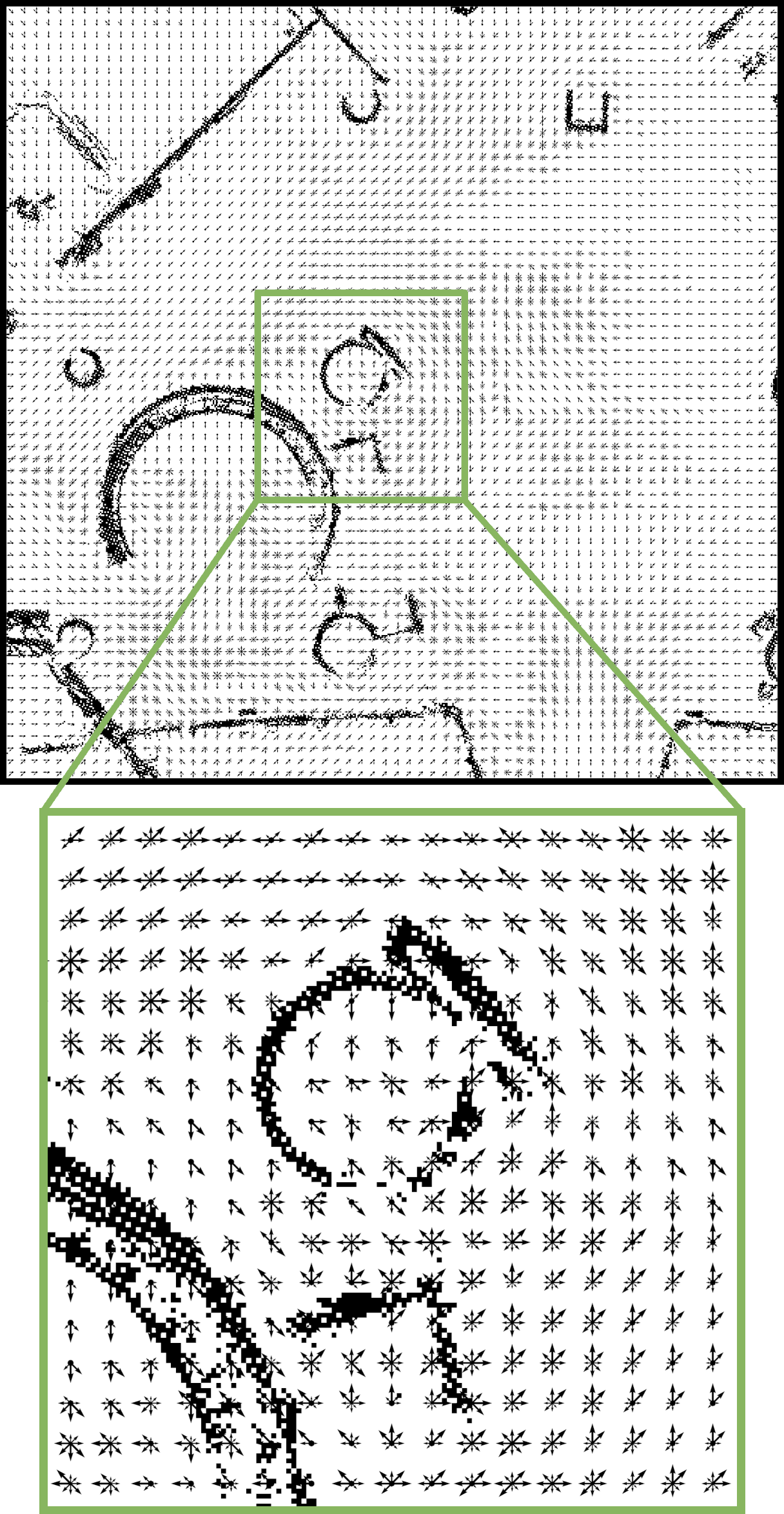
(a) ATC

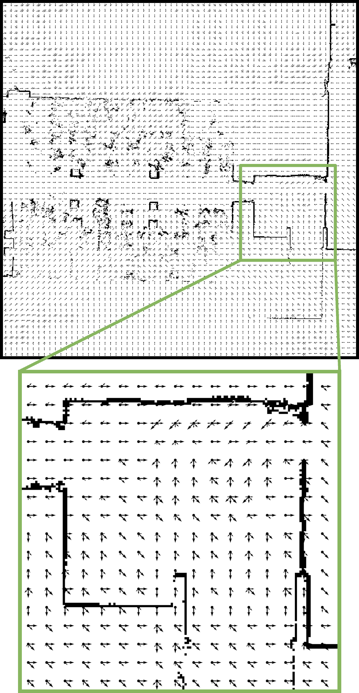
(b) KTH

Figure 1: We learn the correlation between human dynamics and architectural geometry from real people trajectories in environment (a), then we use the same model to estimate human trajectories in an unseen environment (b) without additional data. Below each image, the area marked in green is magnified.

In this work we explore a novel approach to learning people dynamics from environment geometry, in which we train a model on real human data in a real large-scale environment and evaluate the capability of the learned model to transfer across environments. An illustration of the approach is given in Fig. 1.

In particular, the main contributions of this work are:

1. A novel approach for training deep transition probability models from real data;

2. A study over the ability of the proposed approach to predict real unseen human trajectories both in the same environment it was trained on, as well as in a completely different large-scale environment never seen during training;

3. A comparison of the performance of the method against a traditional MoD approach;

4. The first openly available source code and trained models to learn MoDs from geometry.

II Related work

The observation that people tend to follow spatial or spatiotemporal patterns enabled the development of MoDs. MoDs are a special case of semantic maps, where information about motion patterns is retained as a feature of the environment. The existing representations can be split into three groups [2]: (1) trajectory maps, where the information about the motion patterns is retained as a mixture model over the trajectory space [7, 8]; (2) directional maps, where dynamics are represented as a set of local mixture models over velocity space [9, 2, 10]; and (3) configuration changes maps, in contrast to previously mentioned maps, this type of representations does not retain information about motion but instead, it presents the pattern of changes caused by semi-static objects [11, 12].

In this work, we are especially focusing on directional maps, which are well suited to represent local dynamic patterns caused by directly observed moving agents while being robust against partial or noisy observations. Furthermore, this type of MoDs consists of a large spectrum of representations of varying levels of expressiveness and complexity. Including fairly simple models such as floor fields [13] as well as more complex multimodal, continuous representations [14].

It is also important to emphasize that, dynamics do not exist in a vacuum but are affected by environmental conditions, primarily by the environment’s geometry. This idea was initially presented by Helbing and Molnar [15] and later successfully utilized to solve the problem of motion prediction [16].

Even though the idea of utilizing metric information to inform dynamics has substantially impacted the motion prediction community it has not yet received adequate attention in the field of MoDs. One of the more impactful attempts in this direction is the work by Zhi et al. [4]. In that work, the authors utilize artificially generated trajectories to train a deep neural network to predict possible behaviors in new unobserved environments.

At this same time, Doelinger et al. [5, 6] proposed a method to predict not the motion itself but the levels of possible activity in given environments, based on surrounding geometry. Both works by Zhi et al. [4] and Doelinger et al. [5, 6] present important steps towards the prediction of motion patterns given the environment geometry.

However, the aforementioned contributions are application specific and narrow in scope, using either only synthetic data, or by being limited to only small environments. In this work, we propose a step change with respect to the presented state-of-the-art by presenting a way to leverage real human trajectories in large-scale environments and open new possibilities for predicting not only motion patterns but other environment-dependent semantics.

III Method

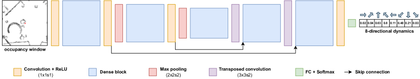
Figure 2: The network used in this work to map from 64$\times$64 occupancy windows to transition probabilities at the center of the window (marked in red)

Let us represent the environment $\mathbf{M}$ the robot is operating in as a collection of cells $c\in\mathbf{M}$. For each cell $c$, we assume to know an occupancy probability $s(c)\in[0,1]$ describing the likelihood of that portion of the environment to be occupied. We refer to $s$ as the static occupancy map of the environment built following [17].

To model people movement in the environment, for each cell $c$, we want to determine the likelihood that a person in $c$ will head in a particular direction $\delta\in[0,2\pi)$ rad. Formally, we define the transition model for cell $c$ as a categorical distribution over $k$ discrete directions equally dividing the range $[0,2\pi)$ rad, i.e.,

$$\mathsf{P}(\delta\mid\mathbf{d}_{c})=\sum_{i=1}^{k}d_{ic}{\mathbf{1}_{i}(\delta)}\enspace,$$ (1)

where $\mathbf{d}_{c}=(d_{1c},\dots,d_{kc}\mid\sum_{i=1}^{k}d_{ic}=1)$, $d_{ic}$ represents the probability of moving toward direction $i$ from $c$, and the indicator function $\mathbf{1}_{i}(\delta)=1$ iff $\frac{2(i-1)}{k}\pi\leq\delta<\frac{2i}{k}\pi$, $0$ otherwise. We use $\mathbf{d}_{c}$ as shorthand for $\mathbf{d}(c)$. We refer to the complete model $\mathbf{d}$ as the map of dynamics (or people flow map) of the environment.

The main assumptions in this work are that: (i) an environment’s geometry around a certain location (i.e., that location’s neighborhood) influences how people move from it; and (ii) neighborhoods having similar occupancy, even from different environments, influence people movement similarly. Under these assumptions, given a certain neighborhood $\mathbf{N}_{c_{r}}\subset\mathbf{M}$ around a reference cell $c_{r}$ our first target is to learn a mapping function $f(\mathbf{w}_{c_{r}})\approx\mathbf{d}_{c_{r}}$, where $\mathbf{w}_{c_{r}}=\{s(c)\mid c\in\mathbf{N}_{c_{r}}\}$, i.e., a window over the occupancy map describing the geometry of the environment around $c_{r}$. Secondly, we want to show the generalization capabilities of $f$, such that, given a different environment $\mathbf{M}^{\prime}$, and a reference cell $c^{\prime}_{r}\in\mathbf{M}^{\prime}$, $f(\mathbf{w}_{c^{\prime}_{r}})\approx\mathbf{d}_{c^{\prime}_{r}}$

III-A Network structure

In practice, we learn $g_{\theta}\approx f$, i.e., a parametric approximation of $f$ defined by the parametrization $\theta$, that we model as a FC-DenseNet architecture [18] following previous literature [5, 6]. The structure of the network is shown in Fig. 2. The network takes as input a 64$\times$64 window over an occupancy grid map, processes it over several densely connected blocks of convolutional layers and max-pooling layers, before upsampling it through transposed convolutions and outputing the $k$-dimensional transition probability distribution $\mathbf{d}_{c_{r}}$, with $c_{r}$ being the center pixel of the input window. In this study we use $k=8$ in order to model the probability of moving in the direction of each of the eight neighboring cells to $c_{r}$. Please refer to [18] for the exact composition of the dense blocks.

One thing to note is that most occupancy grid maps are built at very high resolution (usually 0.05 to 0.1 m), but for MoDs modelling human traffic, those resolutions are too dense, and they are usually constructed at around 0.4 to 1 m per cell [2]. Therefore, to be able to build models at arbitrary output grid resolutions, we match the grid size for the input of the network, by interpolating from the original grid resolution of the occupancy map. This means that, for example, if we want the network to learn a people flow map at a 0.4 m/cell resolution, the 64$\times$64 input window covers an area of 25.6 m².

III-B Training and augmentations

We train $g_{\theta}$ in a supervised fashion by using a dataset of pairs $(\mathbf{w}_{c},\mathbf{\hat{d}}_{c})$ of occupancy windows $\mathbf{w}_{c}$ with their corresponding groundtruth transitions $\mathbf{\hat{d}}_{c}$ (more details in Sec. III-C). As loss we use mean squared error (MSE) between the predicted transition probabilities and the groundtruth. We train for 100 epochs, using Adam as optimizer with a fixed learning rate of 0.001.

To extend the amount of available data, we augment each input-output pair randomly by vertical and/or horizontal flipping followed by a random rotation of either $0$, $\frac{1}{2}\pi$, $\pi$, or $\frac{3}{2}\pi$ rad, with equal probability. When we perform these augmentations, the groundtruth transition probabilities are transformed accordingly to still match the transformed input window.

III-C Datasets

The dataset we use for training our model is the ATC Dataset, containing real pedestrian data from the ATC mall (The Asia and Pacific Trade Center, Osaka, Japan, first described by [19]). This dataset was collected with a system consisting of multiple 3D range sensors, covering an area of about 900 m². The data has been collected between October 24, 2012 and November 29, 2013, every week on Wednesday and Sunday between 9:40 and 20:20, which gives a total of 92 days of observation. For each day a large number of human trajectories is recorded. An occupancy grid map of the environment $s^{A}$ at 0.05 m/pixel resolution is also available with the dataset.

From the ATC dataset, we picked Wednesday November 14, 2012 for training and Saturday November 18, 2012 for testing, which we will refer to as ATC-W and ATC-S respectively. For each day, we built a groundtruth MoD using the floor field algorithm [13] which constructs a per-cell 8-directional transition model by accumulation directly from trajectory data. We refer to these models as $\mathbf{\hat{d}}^{W}$ and $\mathbf{\hat{d}}^{S}$ respectively. For training then, we will use a dataset composed of 1479 pairs of cells $(\mathbf{w}_{c},\mathbf{\hat{d}}^{W}_{c})$, while a dataset of 1360 pairs $(\mathbf{w}_{c},\mathbf{\hat{d}}^{S}_{c})$ will be used for validation. In both, $\mathbf{w}_{c}$ is a window around cell $c$ extracted from $s^{A}$.

As dataset representing an unseen environment, we use the KTH Track Dataset [20], which we will refer to as KTH. Data from this dataset is never seen during training and is only used for evaluation. In this dataset, 6251 human trajectory data were collected by an RGB-D camera mounted on a Scitos G5 robot navigating through University of Birmingham library. An occupancy grid map of the environment $s^{K}$ at 0.05 m/pixel resolution is also available with the dataset. Similarly to ATC, for this dataset we learn a floor field model $\mathbf{\hat{d}}^{K}$ which we will consider the goal standard for the performance on this dataset.

IV Experiments

In order to evaluate the proposed method, we mainly want to assess:

1. how well can the learned model predict human trajectories within the same environment, but on a different day (ATC-S);

2. how well can the model transfer to a different environment entirely (KTH);

3. what effect has the choice of grid resolution on generalization performance.

In both experiments, we want to compare the performance of the trained transition model against the goal standard model, i.e., the floor field model built using the trajectories from that testing environment. Moreover, we are testing two different grid resolution for the network, specifically 0.4 and 0.8 m/cell, to measure the impact of grid resolution on the generalization performance.

As metric, we will compute the likelihood for trajectories contained in a dataset to be predicted by each model. Formally, each trajectory $\tau$ is a sequence of points defined by their $xy$-coordinates and the angle $\delta\in[0,2\pi)$ between consecutive points, i.e., $\tau=[(x_{1},y_{1},\delta_{1}),\dots,(x_{n},y_{n},\delta_{n})]$. Then, given a transition model $\mathbf{d}$, the average likelihood for the trajectory $\tau$ is computed as

$$\mathcal{L}(\tau\mid\mathbf{d})=\frac{1}{n}\sum^{n}_{i=1}\mathsf{P}(\delta_{i}\mid\mathbf{d}_{c_{i}})\enspace,$$ (2)

where $\mathbf{d}_{c_{i}}$ refers to the transition model for the grid cell ${c_{i}}$ containing the coordinates $(x_{i},y_{i})$, and $\mathsf{P}(\delta_{i}\mid\mathbf{d}_{c})$ is computed following (1).

TABLE I: Average trajectory likelihoods and percentages of the range between lower and upper bounds.

	ATC-S		KTH
Model	$\mathcal{L}$	%	$\mathcal{L}$	%
uniform	0.125	0.0	0.125	0.0
Ours (0.8 m/cell)	0.195	62.0	0.140	13.9
Ours (0.4 m/cell)	0.199	65.5	0.211	79.6
$\mathbf{\hat{d}}^{W}$	0.220	84.1	-	-
$\mathbf{\hat{d}}^{S}$	0.238	100.0	-	-
$\mathbf{\hat{d}}^{K}$	-	-	0.233	100.0

Tab. I contains the average trajectory likelihood for each method. The performance by $\mathbf{\hat{d}}^{S}$ and $\mathbf{\hat{d}}^{K}$ serve as the upper bound of performance achievable on their respective dataset, since they are model built directly from the same set of trajectories they are now predicting. On the other hand, as lower bound on performance, we consider the “uniform” model, i.e., an uninformed model where $\forall c_{i}\,\mathbf{d}_{c_{i}}=(\frac{1}{8},\frac{1}{8},\frac{1}{8},\frac{1}{8},\frac{1}{8},\frac{1}{8},\frac{1}{8},\frac{1}{8})$. For each method, we also report the percentage of performance considering the range between lower and upper bounds, computed as

$$\frac{\text{model}-\text{uniform}}{\text{upper}-\text{uniform}}\times 100\enspace,$$ (3)

where “upper” is $\mathbf{\hat{d}}^{S}$ for ATC-S and $\mathbf{\hat{d}}^{K}$ for KTH.

When considering ATC-S, i.e., the same environment the network was trained on, but using trajectories from a different day, the proposed method performs worse than the traditional model it was trained on ($\mathbf{\hat{d}}^{W}$). This can be explained by the fact that for areas where the geometry of the environment alone is insufficient to disambiguate among different human behaviours, the networks proposes an average solution, while the traditional floor field model, being fully local, retains information about the specificity of each section of the environment.

When looking at the generalization capabilities of our proposed method on the unseen KTH environment, we can make a couple of observations. First, generalization seems highly impacted by grid resolution, with the method working with a larger grid being unable to generalize, while the denser one can. This can be due to the fact that larger grid means also larger input window, meaning easier overfitting to the specific geometry of the training environment.

On the other hand, the method working at 0.4 m/cell is able to generalize and model people behaviour across environments without loss of performance. This is a remarkable result that will require more thorough study to be properly confirmed, but this initial study hints at the fact that learning MoDs from architectural geometry, across environments, is possible. One more time, it is worth pointing out, that the reason for the missing data in Tab. I is due to inability of traditional models to transfer between environments, which our work addresses.

V Conclusions

In this work, we presented a novel approach to infer maps of dynamics (MoDs) from architectural geometry and transfer the learned model to new unseen environments. We evaluated the generalization ability of the proposed method on real human trajectories in different large-scale environments, showing that, when tasked to predict trajectories across environments, the proposed method performed at the same level of performance shown in the training environment.

In the future, it will be interesting to research if similar generalization can be obtained with other MoD methods. Also, the possibility of integrating the proposed approach with traditional MoD algorithms in the form of a prior is exciting, as where the proposed method estimates an average behaviour from the geometry of the environment, traditional methods can be used to refine the model to the specifics of each different environment.

In conclusion, while these results are currently somewhat limited in scope, the ability of the proposed method to generalize to unseen large-scale buildings is unprecedented in MoDs literature, which makes this study a possible stepping stone towards new directions in robotic mapping.

References

- [1] T. Kruse, A. K. Pandey, R. Alami, and A. Kirsch, “Human-aware robot navigation: A survey,” Robotics and Autonomous Systems, vol. 61, no. 12, pp. 1726–1743, 2013.
- [2] T. P. Kucner, A. J. Lilienthal, M. Magnusson, L. Palmieri, and C. S. Swaminathan, Probabilistic Mapping of Spatial Motion Patterns for Mobile Robots. Springer International Publishing, 2020.
- [3] T. Lai, W. Zhi, and F. Ramos, “Occ-traj120: Occupancy maps with associated trajectories,” CoRR, 2019.
- [4] W. Zhi, T. Lai, L. Ott, and F. Ramos, “Trajectory Generation in New Environments from Past Experiences,” in 2021 IEEE/RSJ International Conference on Intelligent Robots and Systems (IROS), Sep. 2021, pp. 7911–7918.
- [5] J. Doellinger, M. Spies, and W. Burgard, “Predicting Occupancy Distributions of Walking Humans With Convolutional Neural Networks,” IEEE Robotics and Automation Letters, vol. 3, no. 3, pp. 1522–1528, Jul. 2018.
- [6] J. Doellinger, V. S. Prabhakaran, L. Fu, and M. Spies, “Environment-Aware Multi-Target Tracking of Pedestrians,” IEEE Robotics and Automation Letters, vol. 4, no. 2, pp. 1831–1837, Apr. 2019.
- [7] M. Bennewitz, W. Burgard, and S. Thrun, “Using em to learn motion behaviors of persons with mobile robots,” in IEEE/RSJ International Conference on Intelligent Robots and Systems, vol. 1, 9 2002, pp. 502–507 vol.1.
- [8] B. T. Morris and M. M. Trivedi, “A survey of vision-based trajectory learning and analysis for surveillance,” IEEE Transactions on Circuits and Systems for Video Technology, vol. 18, no. 8, pp. 1114–1127, 8 2008.
- [9] R. Senanayake and F. Ramos, “Bayesian hilbert maps for dynamic continuous occupancy mapping,” in Proceedings of the 1st Annual Conference on Robot Learning, ser. Proceedings of Machine Learning Research, S. Levine, V. Vanhoucke, and K. Goldberg, Eds., vol. 78. PMLR, 2017, pp. 458–471.
- [10] S. Molina, G. Cielniak, T. Krajník, and T. Duckett, “Modelling and predicting rhythmic flow patterns in dynamic environments,” in Towards Autonomous Robotic Systems, M. Giuliani, T. Assaf, and M. E. Giannaccini, Eds. Cham: Springer International Publishing, 2018, pp. 135–146.
- [11] T. Krajnik, J. Pulido Fentanes, J. Santos, T. Duckett et al., “Frequency map enhancement: Introducing dynamics into static environment models,” ICRA Workshop AI for Long-Term Autonomy, 2016.
- [12] J. Saarinen, H. Andreasson, and A. J. Lilienthal, “Independent Markov chain occupancy grid maps for representation of dynamic environment,” in 2012 IEEE/RSJ International Conference on Intelligent Robots and Systems, Vilamoura, 2012.
- [13] C. Burstedde, K. Klauck, A. Schadschneider, and J. Zittartz, “Simulation of pedestrian dynamics using a two-dimensional cellular automaton,” Physica A: Statistical Mechanics and its Applications, vol. 295, no. 3, pp. 507–525, 2001.
- [14] T. P. Kucner, M. Magnusson, E. Schaffernicht, V. H. Bennetts, and A. J. Lilienthal, “Enabling flow awareness for mobile robots in partially observable environments,” IEEE Robotics and Automation Letters, vol. 2, no. 2, pp. 1093–1100, 4 2017.
- [15] D. Helbing and P. Molnar, “Social force model for pedestrian dynamics,” Physical review E, vol. 51, no. 5, p. 4282, 1995.
- [16] A. Rudenko, L. Palmieri, M. Herman, K. M. Kitani, D. M. Gavrila, and K. O. Arras, “Human motion trajectory prediction: A survey,” The International Journal of Robotics Research, vol. 39, no. 8, pp. 895–935, 2020.
- [17] H. Moravec and A. Elfes, “High resolution maps from wide angle sonar,” in 1985 IEEE International Conference on Robotics and Automation Proceedings, Mar. 1985, pp. 116–121.
- [18] S. Jégou, M. Drozdzal, D. Vazquez, A. Romero, and Y. Bengio, “The One Hundred Layers Tiramisu: Fully Convolutional DenseNets for Semantic Segmentation,” arXiv:1611.09326 [cs], Oct. 2017.
- [19] D. Brščić, T. Kanda, T. Ikeda, and T. Miyashita, “Person tracking in large public spaces using 3-d range sensors,” IEEE Transactions on Human-Machine Systems, vol. 43, no. 6, pp. 522–534, 2013.
- [20] C. Dondrup, N. Bellotto, F. Jovan, and M. Hanheide, “Real-Time Multisensor People Tracking for Human-Robot Spatial Interaction,” in International Conference on Robotics and Automation (ICRA) - Workshop on Machine Learning for Social Robotics, 2015.