How to train your solver: Verification of boundary conditions for smoothed particle hydrodynamics

Abstract

The weakly compressible smoothed particle hydrodynamics (WCSPH) method has been employed to simulate various physical phenomena involving fluids and solids. Various methods have been proposed to implement the solid wall, inlet/outlet, and other boundary conditions. However, error estimation and the formal rates of convergence for these methods have not been discussed or examined carefully. In this paper, we use the method of manufactured solution (MMS) to verify the convergence properties of a variety of commonly employed of various solid, inlet, and outlet boundary implementations. In order to perform this study, we propose various manufactured solutions for different domains. On the basis of the convergence offered by these methods, we systematically propose a convergent WCSPH scheme along with suitable methods for implementing the boundary conditions. We also demonstrate the accuracy of the proposed scheme by using it to solve the flow past a circular cylinder. Along with other recent developments in the use of adaptive resolution, this paves the way for accurate and efficient simulation of incompressible or weakly-compressible fluid flows using the SPH method.

1 Introduction

The Smoothed particle hydrodynamics (SPH) method is widely used to solve fluid dynamics problems[1]. One of the widely used variants of the SPH method is the weakly compressible SPH (WCSPH). In WCSPH, the pressure is obtained using an artificial equation of state [2]. Many WCSPH schemes viz. transport velocity formulation (TVF) [3], entropically damped artificial compressibility (EDAC) SPH [4], $\delta^{+}$-SPH [5], and dual-time SPH [6] have been proposed in the last decade. Recently, Negi and Ramachandran [7] introduced several SPH schemes and formally showed the convergence to be second order. However, they only considered domains with periodic boundaries. For these schemes to be useful in practical simulation it is essential to also have second order convergent boundary condition implementations.

In the context of SPH, accurate implementation of boundary conditions is a grand challenge problem [8]. Many authors (See the review by Violeau and Rogers [9]) have proposed various methods to implement solid boundary conditions in SPH. Some authors [10, 11, 12, 3] use few layers of fixed solid (boundary) particles and use different methods to extrapolate the properties from fluid to the solid particles. Colagrossi and Landrini [13] proposed the creation of solid particles by reflecting the fluid particles about the solid-fluid interface and retaining the properties. Marrone et al. [14] used fixed ghost particles to implement the boundary condition wherein a reflection of these ghost particles about the solid-fluid interface are used to evaluate properties on the ghost particles. Recently, Fourtakas et al. [15] proposed to use a dynamically generated local stencil for the particles near the boundary. Some authors [16, 17, 18, 19] propose to use a single layer of particles to represent the solid boundary and use methods to correctly evaluate the forces. Others like Ferrand et al. [17] proposed semi-analytical methods to compensate for the loss of kernel support near the boundary.

For the case of open boundaries, the use of a weakly compressible formulation poses unique problems since pressure waves travel with an artificial speed of sound. These waves must pass through the open boundaries without reflecting into the domain. Federico et al. [20] propose a do-nothing kind of outlet where the fluid particles are converted from fluid to outlet particles while retaining their properties. Tafuni et al. [21] propose to mirror the inlet and outlet particles to calculate properties and its gradient. The inlet and outlet properties are set using a Taylor series expansion from the respective ghost particle to the inlet/outlet particle. Recently, Negi et al. [22] proposed a modified version of the method proposed by Lastiwka et al. [23] where a time-averaged value is passed to the inlet/outlet and properties derived from the characteristics of the flow are added using a Shepard interpolation [24]. Many authors [22, 11, 25] compared various boundary condition implementations qualitatively without performing a convergence study. Furthermore, in the context of SPH, the errors are often shown qualitatively by comparing the results of the simulation [3, 4, 5].

In this paper, we verify the convergence of various boundary condition implementations that have been proposed and identify second-order convergent methods that are suitable for use for the most common solid wall, as well as inlet and outlet boundary conditions. In order to identify a convergent boundary implementation, we use the method of manufactured solutions (MMS) introduced by Negi and Ramachandran [26] for SPH. In MMS, a manufactured solution (MS) is created such that the boundary condition is satisfied at the boundary interface of interest. Since the MS is not a solution of the weakly compressible Navier-Stokes (NS) equation, we obtain a residue on substituting the MS in the NS equations. This residue is added as a source term to the NS equation in the scheme and it is expected that the solver will recover the MS as the solution. In order to test the boundary condition, one requires a convergent scheme in the bulk of the fluid for which we use the second-order convergent scheme proposed by Negi and Ramachandran [7] which is further verified using MMS in [26].

We believe that this is the first time that second order convergent boundary condition implementations have been identified and verified in the context of WCSPH. However, the implementation of these methods to solve a real-life problem is non-trivial. In view of that, we propose a complete algorithm and demonstrate the accuracy by solving a simple flow past a circular cylinder problem. This shows that the resulting SPH scheme can be applied to a variety of problems, paving the way for SPH to be an effective alternative to traditional finite volume based codes especially when combined with some recent advancements of adaptive resolution SPH schemes [27, 28].

In the next section, we discuss the SPH method and the second-order discretizations. We then discuss various solid boundary condition implementations, viz. pressure Neumann, slip and no-slip in section 3, and open boundary conditions, viz. inlet and outlet in section 4 for both pressure and velocity. In section 5, we discuss the MMS in general and its construction for specific boundary condition. We compare all the boundary condition implementation in the section 6 followed by conclusion in section 8. All the results in this manuscript are reproducible, and the source code for the simulations can be found at https://gitlab.com/pypr/mms_sph_bc.

2 The SPH method

Chorin [29] proposed the weakly-compressible method to solve fluid flow problems. In the weakly-compressible method, we solve the governing equations given by

$$\begin{split}\frac{d\varrho}{dt}&=-\varrho\nabla\cdot\mathbf{u}\\ \frac{d\mathbf{u}}{dt}&=-\frac{\nabla p}{\varrho}+\nu\nabla^{2}\mathbf{u},\\ \end{split}$$ (1)

where $\varrho$ , $\mathbf{u}$, and $p$ are the density, velocity, and pressure of the fluid, and $\nu$ is the dynamic viscosity of the fluid. Additionally, we use an artificial equation of state (EOS) to link the pressure with the density. In SPH, we use the EOS given by

$$p=c_{o}^{2}(\varrho-\varrho_{o}),$$ (2)

where $\varrho_{o}$ and $c_{o}$ are the reference density and artificial speed of sound, respectively. In this paper, we use the L-IPST-C scheme proposed by Negi and Ramachandran [7] to discretize the governing equations. The continuity equation is discretized as

$$\frac{d\varrho_{i}}{dt}=-\varrho_{i}\sum_{j}(\mathbf{u}_{j}-\mathbf{u}_{i})\cdot\tilde{\nabla}W_{ij}\omega_{j},$$ (3)

where $\tilde{\nabla}W_{ij}$ is the kernel gradient corrected using the correction proposed by Bonet and Lok [30], and $\omega_{j}=\frac{1}{\sum_{j}W_{ij}}$ is the numerical volume. The function $W_{ij}=W(\mathbf{x}_{i}-\mathbf{x}_{j},h_{ij})$ is a smoothing kernel used in SPH, where $\mathbf{x}_{i}$ is the position of the destination particle, $\mathbf{x}_{j}$ is the position of the source particle, and $h_{ij}=0.5(h_{i}+h_{j})$ is the average smoothing radius. The momentum equation is discretized as

$$\frac{d\mathbf{u}_{i}}{dt}=\sum_{j}\left(\frac{(p_{i}-p_{j})}{\varrho_{i}}\tilde{\nabla}W_{ij}\omega_{j}+\nu(\nabla\mathbf{u}_{j}-\nabla\mathbf{u}_{i})\cdot\tilde{\nabla}W_{ij}\omega_{j}\right),$$ (4)

where $\nabla\mathbf{u}_{i}=\sum_{j}(\mathbf{u}_{j}-\mathbf{u}_{i})\otimes\tilde{\nabla}W_{ij}\omega_{j}$. The particles are shifted using the iterative particle shifting technique proposed by Huang et al. [31] after every 10 timesteps. The particle properties are updated after shifting using first-order Taylor series approximation given by

$$\phi(\tilde{\mathbf{x}})=\phi(\mathbf{x})+(\tilde{\mathbf{x}}-\mathbf{x})\nabla\phi(\mathbf{x}),$$ (5)

where $\tilde{\mathbf{x}}$ is the position after shifting, $\mathbf{x}$ is the position before shifting, and $\phi$ is any fluid property. We use a second-order Runge-Kutta time integration scheme to integrate the continuity and momentum equations. Since we are interested in the spatial convergence of the scheme, we use a constant timestep corresponding to the highest resolution, i.e. $500\times 500$ for all the simulations given by

$$\Delta t=\frac{h}{c_{o}+U}=\frac{1.2\times 1/500}{20+1}=0.00012\ sec.$$ (6)

We assume a maximum velocity $U=1m/s$ and corresponding speed of sound $20m/s$ for all our simulations.

In order to apply boundary conditions, many authors have proposed different methods to implement Neumann pressure, slip, and no-slip boundary conditions in SPH. The main objective is to extrapolate velocity and pressure from the fluid particle to the ghost particle representing solid such that the desired condition is satisfied. In the next section, we discuss various boundary conditions in brief.

3 Solid boundary conditions

In this section, we discuss various boundary condition implementations widely used in the SPH literature. We classify these implementations on the basis of the requirement of the secondary particle arrays. In SPH, two types of particles are used to implement boundary conditions, viz. ghost, and virtual particles. The ghost particles carry the extrapolated properties from the fluid and influence the fluid particles. Whereas the virtual particles are used to evaluate some intermediate value of a property from fluid and do not affect the actual flow.

Many authors [17, 16, 32] have proposed different approaches where a single layer of ghost particles are used. In order to assess the effect of the number of layers on the accuracy of the second order accurate gradient and Laplacian discretization, we perform a simple numerical test. In this test, we consider a finite 2D domain of size $1m\times 1m$. We discretize the domain using particles at different resolutions, and initialize various properties using

$$\begin{split}u(x,y)&=\sin(4\pi(x+y)),\\ v(x,y)&=\cos(4\pi(x+y)),\\ p(x,y)&=sin(4\pi x)+sin(4\pi y).\end{split}$$ (7)

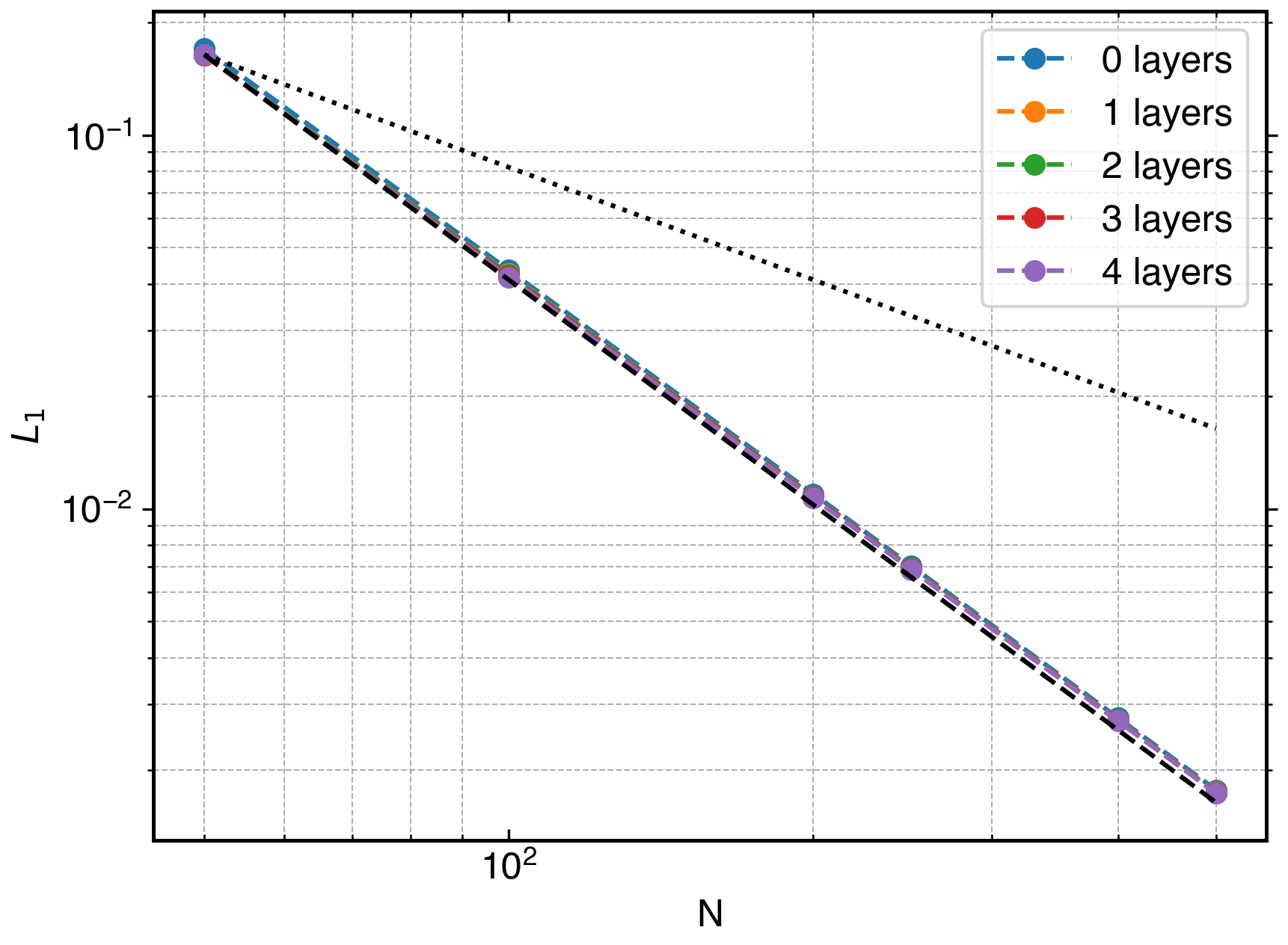
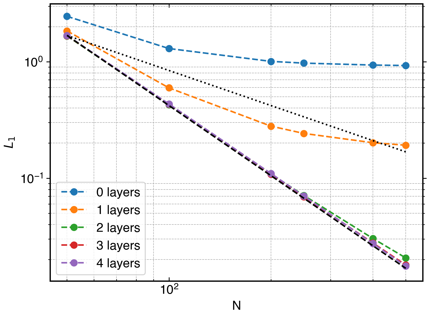
Figure 1: $L_{1}$ error in pressure gradient (left) and Laplacian (right) approximation with change in the skipped number of layers.

We compute the SPH approximation of the pressure gradient and Laplacian of velocity on the particles using the discretization in eq. 4. Since the particles near the boundary do not have complete support, they will have higher errors compared to the inner particles. We compute the $L_{1}$ error in the approximation using

$$L_{1}(N_{p})=\frac{\sum_{j}^{N_{p}}|f_{j}(\mathbf{x})-\tilde{f}(\mathbf{x})|}{N_{p}},$$ (8)

where $f(x)$ is the computed value and $\tilde{f}(\mathbf{x})$ is the actual value, $N_{p}$ are the number of particles in the domain $(1-2n\Delta x)\times(1-2n\Delta x)$, where $n$ is the number of layers skipped from each side. In fig. 1, we plot the $L_{1}$ error for the particles skipping $n$-layers of particles from the outermost boundary for pressure gradient and Laplacian approximations. We note that both the discretization used are second-order accurate in a periodic domain [7]. However, we observe that the pressure gradient is second-order accurate even when zero layers of particles are surrounding the domain of interest. Whereas, for the Laplacian approximation, we require at least 2 layers of particles. Since all the second-order accurate formulations for Laplacian approximation require gradient on all the neighboring particles [7] therefore the requirement for the number of neighboring particles is double to that in the case of the gradient approximation for the second-order accurate convergence.

This numerical test shows that the boundary implementation which uses a single layer of particles is bound to have error in Laplacian approximation resulting in an inaccurate solution irrespective of having an accurate boundary condition implementation. Furthermore, since all the second order viscosity formulations require the evaluation of gradient on the boundary particle [7], we do not pursue the implementation of boundaries based on the local point symmetry method in [33, 34, 15] for the no-slip boundary condition. The various solid boundary implementations considered are as follows:

3.1 Using a single layer of ghost particles on the boundary surface

3.1.1 With virtual particles

In these methods, only one layer of particles are used on the boundary surface. Marongiu et al. [32] proposed a characteristics-based evolution equation for pressure update at these boundary particles are given by

$$\frac{d\varrho}{dt}=c_{o}\frac{\partial\varrho}{\partial n}-\varrho\frac{\partial u_{n}}{\partial n}-\frac{\varrho\mathbf{g}\cdot\mathbf{n}}{c_{o}}$$ (9)

where $\mathbf{n}$ is the normal of the boundary surface pointing into the fluid. In order to evaluate the gradient at the boundary point, five-point finite difference approximation is used. These five points are generated along the normal of the boundary particle at a spacing equal to the average particle spacing represented by black point in fig. 2 for a single particle. The values of the properties at these black points are evaluated using Shepard interpolation [24].

Figure 2: Arrangement of ghost and virtual particles for given fluid particle denoted by blue circles. The dashed line is the boundary surface, red particles are ghost (solid) particles. The black dots are generated to evaluate gradient using finite difference at the red boundary points.

3.1.2 Without virtual particles

Hashemi et al. [16] proposed methods to implement pressure and no-slip boundary conditions using one layer of boundary particles on the surface. However, they do not use any extra set of elements to derive the values on the boundary elements denoted by red particles in the fig. 2. In order to satisfy the no-slip boundary condition the velocity of the red particles is kept the same as the velocity of the solid boundary. Whereas, for pressure boundary implementation, momentum balance is performed along the normal of the boundary surface given by

$$\frac{\nabla p}{\varrho}\cdot\mathbf{n}=-\frac{d\mathbf{u}}{dt}\cdot\mathbf{n}+\frac{\mu\nabla^{2}\mathbf{u}}{\varrho}\cdot\mathbf{n}+\mathbf{g}\cdot\mathbf{n},$$ (10)

where $\mathbf{n}$ is the normal of the boundary surface pointing into the fluid. The eq. 10 is discretized using the second-order consistent approximation to obtain the pressure at $i$^th solid boundary particles are given by

$$p_{i}=\frac{\left(\frac{p_{j}}{\varrho_{i}}\tilde{\nabla}W_{ij}\omega_{j}\right)\cdot\mathbf{n}_{i}-\left<-\frac{d\mathbf{u}}{dt}\cdot\mathbf{n}+\frac{\mu\nabla^{2}\mathbf{u}}{\varrho}\cdot\mathbf{n}+\mathbf{g}\cdot\mathbf{n}\right>_{i}}{\left(\frac{1}{\varrho_{i}}\tilde{\nabla}W_{ij}\omega_{j}\right)\cdot\mathbf{n}_{i}}.$$ (11)

3.2 Using multiple layers of ghost particles outside boundary surface

3.2.1 With virtual particles

Marrone et al. [14] proposed a method where fixed virtual particles are generated by reflecting the ghost particles about the interface. The created particles are illustrated in the fig. 3, where red crosses are the virtual particles and red particles on the right represent the ghost particles. The properties on the ghost particles are set as $\varrho_{g}=\varrho_{v}$, $p_{g}=p_{v}$, and the velocity is set according to the slip or no-slip condition required, where $*_{g}$ represent the property value on ghost particle and $*_{v}$ represent the property value on the corresponding virtual particle. In case of slip, the velocity normal to the wall is reversed, whereas in case of no-slip, the velocity is set negative of the value on the corresponding virtual particle. The properties on the virtual particles are evaluated using

$$f_{i}=\sum_{j}f_{j}\tilde{W}_{ij}\omega_{j},$$ (12)

where $f_{*}$ is the desired property, $\omega_{j}$ is the truncated volume of the fluid particles and $\tilde{W}_{ij}$ is the kernel corrected using the method by Liu and Liu [35]. The sum $j$ is taken over all the fluid particles in the support of the kernel,

Figure 3: Arrangement of ghost and virtual particle for given blue fluid particles and solid boundary shown by dashed line. The red circle on the right are the ghost particles, and the red crosses are created by reflecting the ghost about the interface.

3.2.2 Without virtual particles

In SPH literature, most of the methods for boundary condition implementation use multiple layers of ghost particle such that the kernel has full support. Takeda et al. [10] proposed to extrapolate the properties using a linear interpolation depending upon the distance of the ghost particle from the nearest fluid particle as shown in fig. 4. The extrapolated velocity is given by

$$\mathbf{u}_{j}=-\mathbf{u}_{i}\frac{r_{j}-r_{o}}{r_{o}-r_{i}},$$ (13)

where $r_{j}-r_{o}$ and $r_{o}-r_{i}$ are the distances along the normal from the boundary for $j$^th ghost and $i$^th fluid particle, respectively. We select the nearest fluid particle for a particular ghost particle along the normal of the boundary.

Figure 4: Arrangement of particles for the method proposed by Takeda et al. [10]. The ghost particles are shown in red, and the fluid are shown in blue color particles. The value on the red particles are interpolated using the nearest fluid particle along the normal of the boundary surface.

Randles and Libersky [12] proposed a boundary condition for pressure. The prescribed value is assigned to the ghost particles in red and the values on the light blue fluid particles as shown in fig. 5 are set such that the desired condition is satisfied. The value on light blue fluid particles is given by

$$p_{i}=p_{bc}+\frac{\sum_{j\in I}(p_{j}-p_{bc})W_{ij}\omega_{j}}{1-\sum_{j\in B}W_{ij}\omega_{j}},$$ (14)

where $I$ is the set of blue particles, $B$ is the set of red particle, and pressure is evaluated at each $i$^th light blue particle shown in fig. 5.

Figure 5: Arrangement of particles for the method proposed by Randles and Libersky [12], and Adami et al. [36] for the fluid particles in blue and boundary interface shown by dashed line. The red circles on the left represents the ghost solid particles. The property of light blue fluid particle is manipulated to satisfy boundary condition.

Adami et al. [36] proposed the method where Shepard interpolation is employed to extrapolate properties from fluid to ghost particles. The property at a ghost particle is given by

$$f_{i}=\frac{\sum_{j}f_{j}W_{ij}}{\sum_{j}W_{ij}},$$ (15)

where sum $j$ is over all the fluid particles in the support of the kernel as shown by red dashed circle in fig. 5, at the $i$^th ghost particle. Furthermore, Esmaili Sikarudi and Nikseresht [37] proposed to perform a first order accurate extrapolation to evaluate properties on ghost particles.

Colagrossi and Landrini [13] proposed to mirror the fluid particles near the solid interface, about the interface to generate ghost particles as shown in fig. 6. These ghost particles carry the velocity of opposite sign to implement no penetration. The value of pressure and density is kept the same. In order to implement this method, we create new particles for solids from the fluid particles before each time step.

Figure 6: Arrangement of particles for the method proposed by Colagrossi and Landrini [13] for the fluid particles in blue, and boundary represent by the dashed line. The ghost particles in red representing solid are created by the mirror reflection about the interface.

4 Open boundary conditions

Open boundary conditions are required to simulate a wind-tunnel kind of simulation in SPH. It consist of an inlet from where the particles are added to the domain, and an outlet from where the particles exits the domain as shown in fig. 7. The particles added to the domain should have prescribed inlet velocity and should not introduce any artifacts in the flow whereas the outlet should remove particles from the flow without affecting the flow. Since we use a weakly-compressible scheme, pressure waves are inevitable. Therefore, the inlet/outlet must have non-reflecting property along with adherence to the boundary condition. In fig. 7, we show a schematic arrangement of the inlet, fluid, and outlet domains. The dashed line in between different regions are the boundary interfaces. The inlet/fluid particles are converted to fluid/outlet particles once they cross the corresponding interface. Many authors [20, 23, 21, 7] have proposed different methods to implement inlet/outlet boundary condition in SPH. Open boundary condition implementations considered in this paper are as follows:

Figure 7: Schematic of the arrangement of fluid with the inlet and outlet particles. The top and bottom are supported by solid particles not shown in the figure.

4.1 Do-nothing

Federico et al. [20] proposed the method to implement outlet boundary where the properties of the fluid particles crossing the fluid-outlet interface are fixed in time. Therefore, the particle, after crossing the interface, advects with a constant velocity.

4.2 Mirror

Tafuni et al. [38] proposed a method applicable to both inlets and outlets. The properties from the fluid are stored on the virtual particles generated by reflecting the inlet/outlet particles about the interface as shown in fig. 8. The desired property and its gradient are evaluated for each mirror particle using a first-order consistent approximation. From the mirror particle, the property of the corresponding outlet/inlet particle is evaluated using

$$f_{o}=f_{i}-\Delta x_{om}\nabla f_{i},$$ (16)

where $f_{i}$ and $\nabla f_{i}$ are the properties on the mirror particle and $x_{om}$ is the distance between the outlet and mirror particle. In addition to this method, we test the convergence of the method when the Taylor series correction is not applied such that the eq. 16 is simplified to

$$f_{o}=f_{i}.$$ (17)

We refer to this method as simple-mirror.

Figure 8: Schematic of the arrangement of fluid with the inlet and outlet particles and their corresponding virtual particles are shown in light red and red, respectively.

4.3 Characteristics

Lastiwka et al. [23] proposed a non-reflecting inlet and outlet boundary implementation using the method of characteristics. The characteristics of the flow are given by

$$\begin{split}J_{1}&=-c_{o}^{2}(\rho-\rho_{ref})+(p-p_{ref}),\\ J_{2}&=\rho c_{o}(u-u_{ref})+(p-p_{ref}),\\ J_{3}&=-\rho c_{o}(u-u_{ref})+(p-p_{ref})i,\\ \end{split}$$ (18)

where $\rho_{ref}$, $u_{ref}$, and $p_{ref}$ are the reference density, velocity, and pressure. These characteristics are extrapolated to the inlet/outlet particles, and the properties are calculated using the extrapolated characteristics are given by

$$\begin{split}\rho&=\rho_{ref}+\frac{1}{c_{o}^{2}}\left(-J_{1}+\frac{1}{2}J_{2}+\frac{1}{2}J_{2}\right),\\ u&=u_{ref}+\frac{1}{2\rho c_{o}}\left(J_{2}-J_{3}\right),\\ p&=p_{ref}+\frac{1}{2}\left(J_{2}+J_{3}\right).\\ \end{split}$$ (19)

In order to implement the inlet boundary $J_{1}$ and $J_{2}$ should be set zero and $J_{3}$ must be extrapolated from the fluid to the inlet particles. Whereas, for outlet $J_{1}$ and $J_{2}$ are extrapolated from the fluid to the outlet, and $J_{3}$ is set to zero. Recently, Negi et al. [22], proposed to obtain the reference value of the properties by taking a time average of properties when the acoustic intensity of the particle is below some prescribed value. This reference value is determined based on the inlet velocity. We refer to this method as hybrid method.

In the next section, we discuss the procedure one should follow for the construction of manufactured solution in the method of manufactured solutions to test boundary condition implementation in the context of SPH.

5 Method of manufactured solutions

It is of utmost importance that the discretization and approximations employed in a solver are of the desired accuracy. Both verification and validation play an essential role to determined the correctness of a solver. In validation, we test whether the intended physics modeled by the differential equation converges as required. Whereas, in verification, we determine whether the discretization of various terms in the governing equation are coded correctly to reflect the intended rate of convergence. The MMS is a verification technique widely used for the verification of finite volume method [39, 40] and finite element method [41] codes. The MMS can also be used to determine specific terms causing a lower order of convergence or if the code has a mistake. Recently, Negi and Ramachandran [26] proposed procedures to apply MMS in the context of SPH. They show various methods to find coding mistakes as well as procedures to obtain manufactured solution (MS) to verify boundary condition implementation at straight boundaries.

In the MMS, we substitute an MS to the governing partial differential equations to obtain a residue. For example, for an MS of the form $\tilde{\mathbf{u}}(x,y,z,t)$, and governing equation $\mathscr{L}\mathbf{u}=g$, where $\mathscr{L}$ is an operator and $g$ is a source term, we obtain

$$\mathscr{R}=\mathscr{L}\tilde{\mathbf{u}}-g$$ (20)

as the residue. We use this residue as a source term in the solver to obtain the MS from the solver. In SPH, the source term can be easily applied to a particle by just substituting the value of the coordinates in the source function. We solve the equations using the solver on a domain with fluid and solid particles. Since we use a second-order convergent scheme to solve the fluid flow, the errors are generated due to the boundary condition implementations only. Therefore, the error at various resolutions shows the rate of convergence of the boundary condition implementation.

In this paper, we construct various MS such that it satisfies the boundary condition on different domain shapes. We take the following steps in order to construct an MS for the boundary $c(x,y)=0$:

1. Construct a base MS such that it satisfies the general requirement of MMS [26] as follows.

   • The MS must be differentiable up to the highest order present in the governing equations.

   • The MS must satisfy the required physics of the governing equation, for example, if the solver requires the density to be continuous, the MS must have continuous density.

   • It must not prevent the successful completion of the solver.

   • It must be bounded in the domain of interest.

2. In the context of SPH, we additionally require the velocity field to be non-solenoidal [26].

3. Modify the property of interest such that the boundary condition at $c(x,y)=0$ is satisfied. For example, for the no-slip boundary only velocity need to be modified.

4. We note that one should ensure that the MS of the property of interest is non-zero on the boundary before the boundary condition is satisfied. For example, if we need $\mathbf{u}\cdot\mathbf{n}$ at the boundary to be zero, we must make sure that $\mathbf{u}\neq 0$ at the boundary.

In appendix A, we discuss the construction of MS for all the methods discussed in this paper. In the next section, we use these MS (defined in appendix A) to test various boundary condition implementation discussed in section 3 and section 4.

6 Results

In this section, we verify the convergence of various boundary condition implementations discussed in section 3 and section 4 using MMS. We first show the convergence of various solid boundary condition implementations followed by the inflow and outflow boundary implementations. For all the test cases, we simulate 100 timesteps for resolutions in the range $100\times 100$ to $500\times 500$, and evaluate the $L_{1}$ error in the domain given by

$$L_{1}=\sum_{j}\sum_{i}\frac{|(f(x_{i},y_{i},t_{j})-f_{o}(x_{i},y_{i},t_{j}))|}{N\times N_{t}}$$ (21)

where $f$ is the property of interest and $f_{o}$ is the property value determined using the MS, $N$ is the number of particles in the domain, $N_{t}$ are number of instances in time. We fix the timestep corresponding to the highest resolutions in order to isolate the error due to boundary condition implementation.

We use the PySPH [42] framework to implement all the methods. All the results presented in this paper are reproducible and can be easily generated using the automation framework automan [43]. In the interest of reproducibility, we provide the entire source code at https://gitlab.com/pypr/mms_sph_bc.

6.1 Comparison of solid boundary condition implementations

In this section, we verify all the solid boundary methods discussed in section 3. The solid boundary can be straight or curved. In this paper, we do not consider a non-smooth geometric features, like a corner. For corners, one requires a discontinuous MS, and at discontinuity the higher order terms fail to show the actual order of convergence. However, the method showing second-order convergence for smooth boundary will perform better than other methods. We consider three types of boundary shapes viz. straight, convex, and concave as shown in fig. 9. The fluid particles are represented by the blue color, and the green color particles represent the ghost particles for which we set the properties using the MS. The orange colored particles are used to verify a particular method. The domain referred to as ‘straight’, the ghost particles in orange have a constant normal. The domain referred to as ‘convex’, the boundary is a convex surface, whereas the domain referred to as ‘concave’, the boundary is a concave surface. We note that both convex and concave domains are identical, however the boundary surfaces of interest are different.

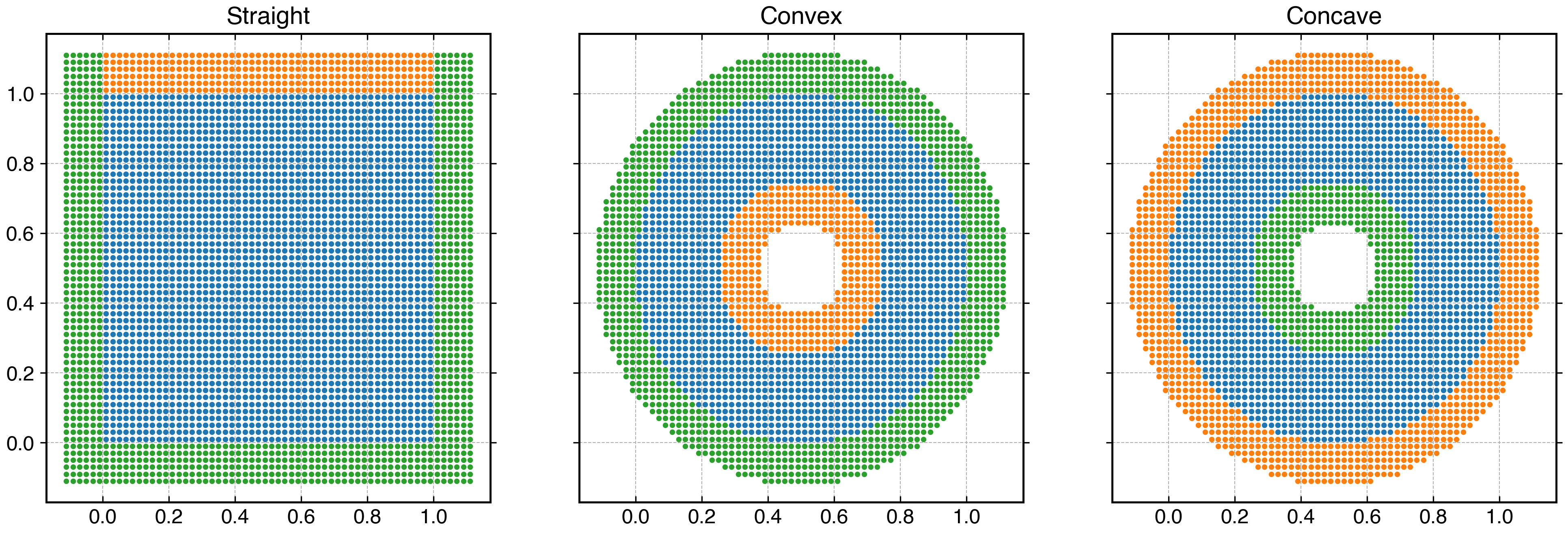
Figure 9: Types of domains considered to test the convergence of solid boundary implementation. The fluid particles are represented by the blue color, the particles in green represent ghost particles on which properties are set using MS, and the particles in orange are used to test the convergence of boundary implementation of interest.

We observe that the convex and concave domains have staircase pattern at the boundary due to the use of the Cartesian arrangement of particles to represent the boundary. We use the method proposed by Negi and Ramachandran [44], to pack the particles near both, the inner and outer surface. In fig. 10, we plot the packed version of the convex and concave domains, and we refer to these as ‘packed-convex’ and ‘packed-concave’ respectively.

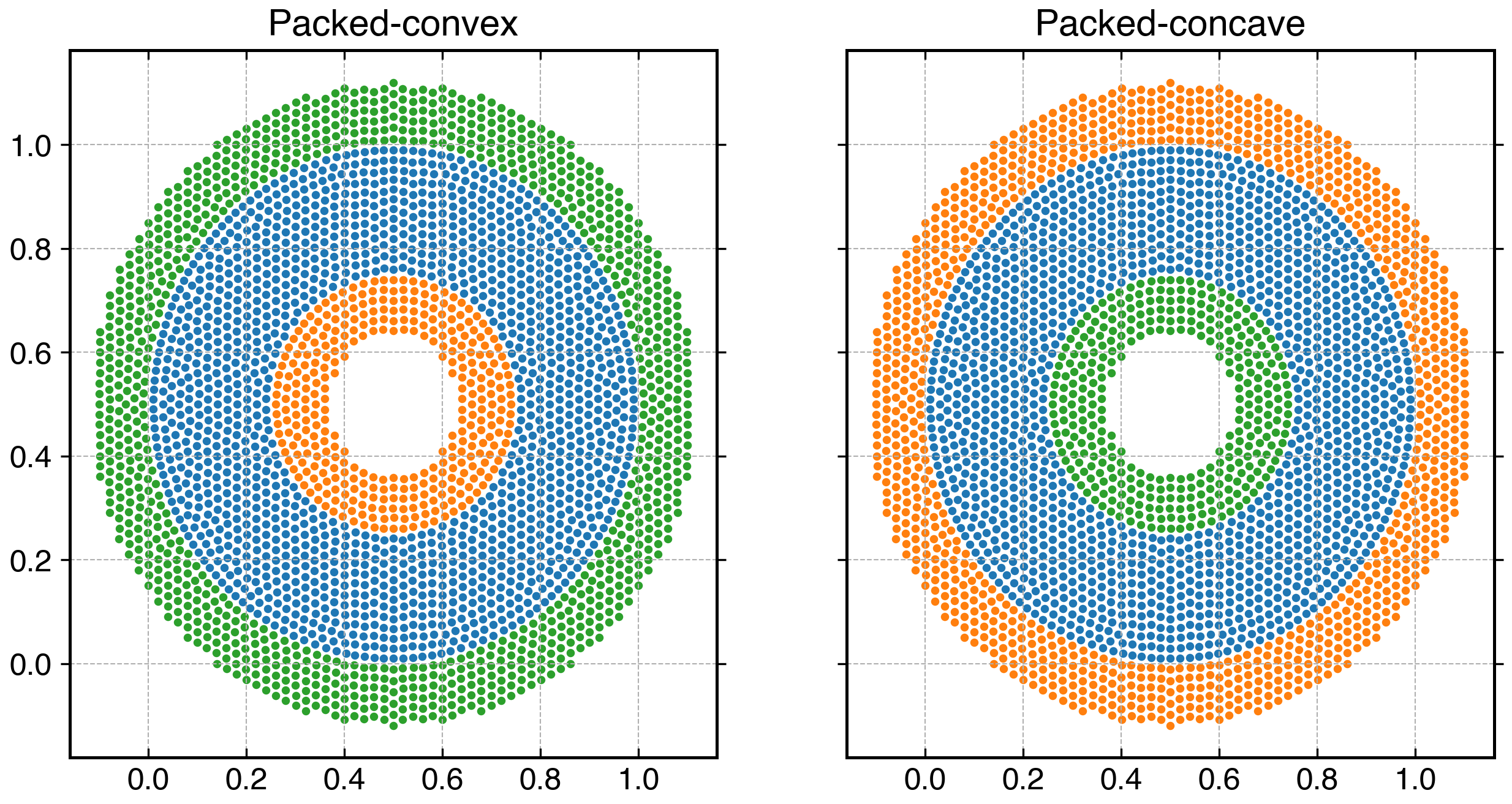
Figure 10: The packed version of convex and concave domains. The fluid particles are represented by blue color, the particles in green represents ghost particles on which properties are set using MS, and the particles in orange are used to test the convergence of desired boundary condition implementation.

6.1.1 Neumann pressure boundary condition

In this section, we apply various methods described in section 3 to apply the Neumann pressure boundary condition on the orange particles shown in the domains in fig. 9, and fig. 10. We first use the MS in eq. 22. The MS ensures that $\nabla p\cdot\mathbf{n}=0$ at the boundary of interest in the straight domain. We refer to a particular method using the corresponding first author names. The ‘MMS’ and ‘MMS-2L’ are the cases where properties on solid are updated using the MS, and six layers and two layers of ghost particles are used to represent solid, respectively. In fig. 11, we plot the $L_{1}$ error in the pressure and velocity after 100 timesteps.

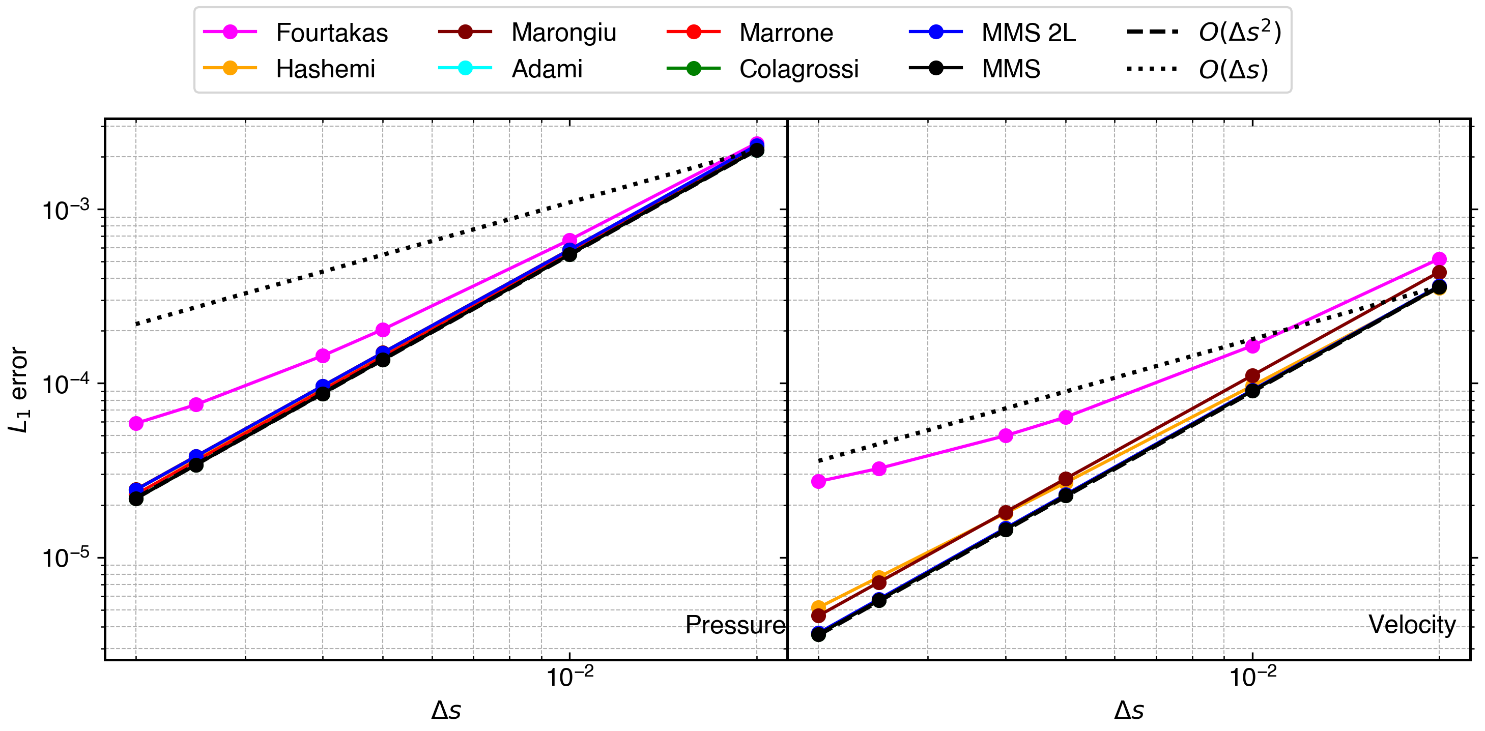
Figure 11: $L_{1}$ error in pressure and velocity after 100 time steps for different Neumann pressure boundary implementations in the straight domain in fig. 9.

The ‘MMS-2L’ plot shows that the L-IPST-C scheme converges even when two layers of solid particles are employed for a straight boundary. In the case of the straight domain, all the methods considered in this paper are second-order convergent except the method proposed by Fourtakas et al. [15], where a virtual stencil is used to complete the support of the particles. However, the rate of convergence is similar to as reported in [15].

We also test all the methods on the convex and concave domains. In order to verify, we use the MS in eq. 23 which satisfies the boundary condition for the surface of interest in both the domains. In fig. 12, and fig. 13, we plot the $L_{1}$ error for pressure and velocity for the convex and concave domains, respectively.

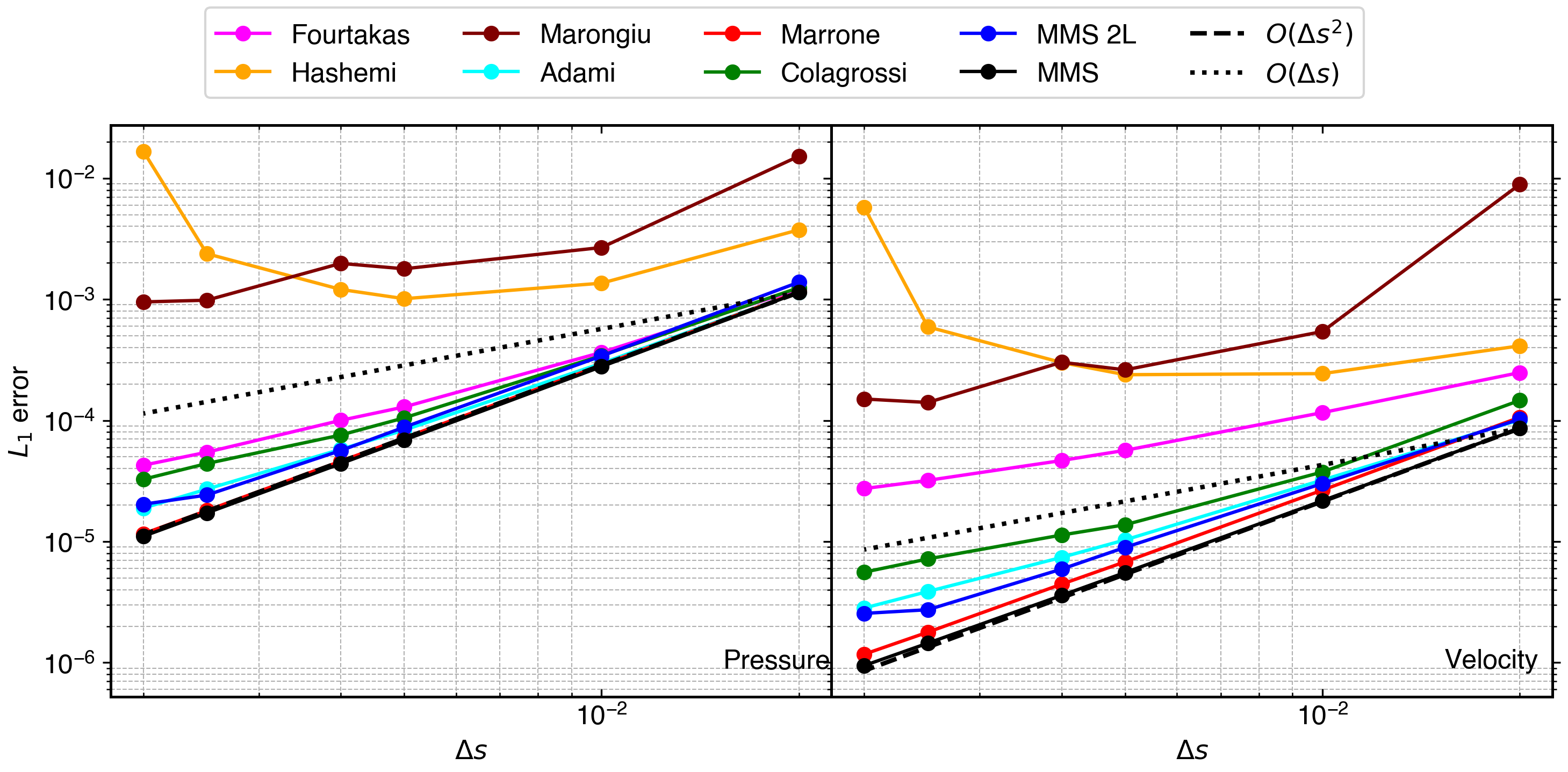
Figure 12: $L_{1}$ error in pressure and velocity after 100 time steps for different Neumann pressure boundary implementations in the convex domain as shown in fig. 9.

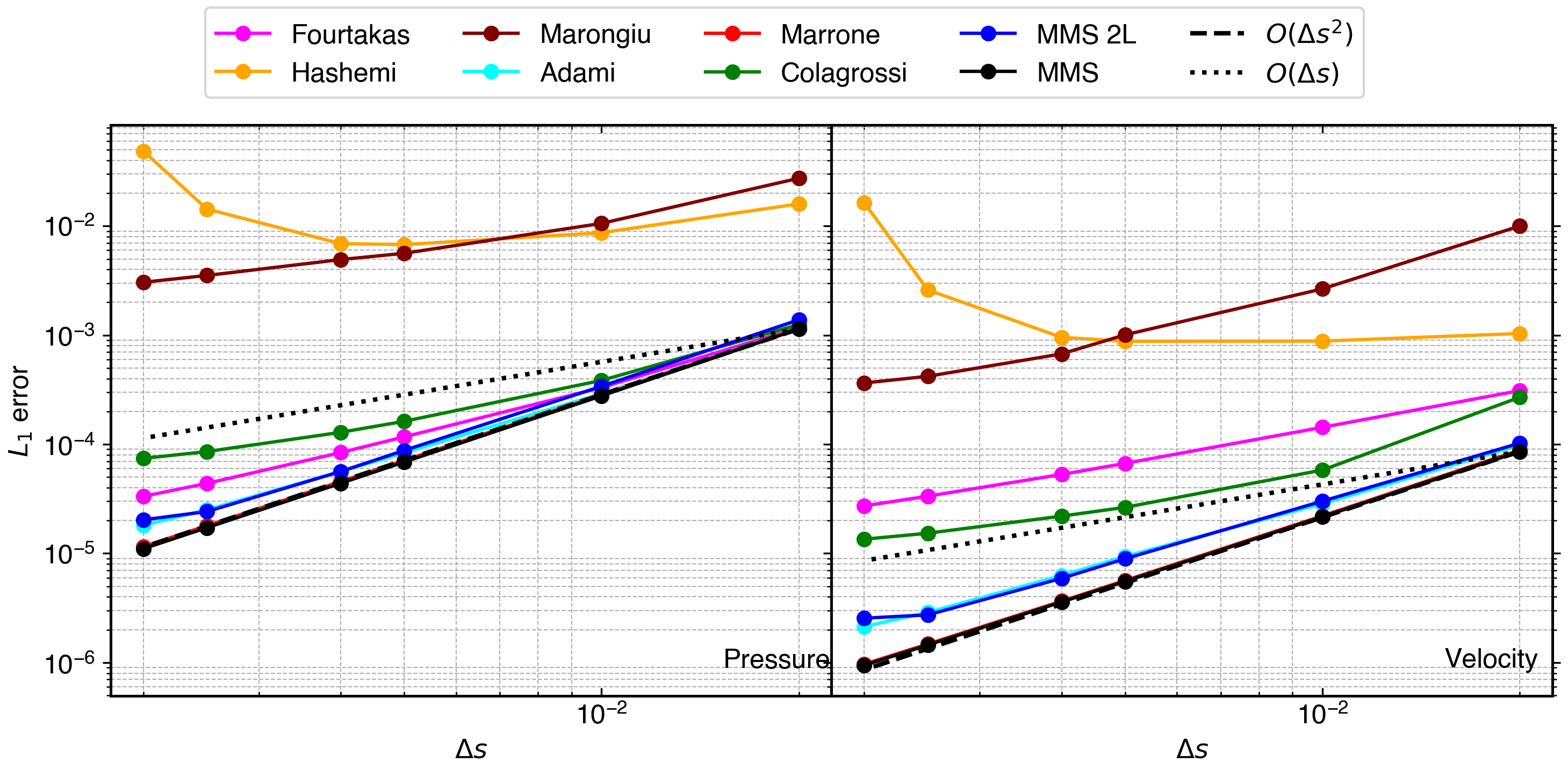
Figure 13: $L_{1}$ error in pressure and velocity after 100 time steps for different Neumann pressure boundary implementations in the concave domain as shown in fig. 9.

We observe that the method proposed by Hashemi et al. [45] diverges since only a single layer of particles are used to represent solid, which is insufficient even for corrected gradient computation. However, the method proposed by Marongiu et al. [32] shows first-order convergence. Moreover, the rate of convergence is non-monotonous for a convex boundary. The reason behind a lower order of convergence is the use of a single layer of particles and zeroth order interpolation on the virtual particles, which are further used in the fifth order finite difference interpolation. The method proposed by Fourtakas et al. [15] shows first order convergence in pressure and 1.5 in velocity as expected. The convergence of the method proposed by Adami et al. [36], and ‘MMS-2L’ are very close to 1.5. The ‘MMS-2L’ has a slight decrease in convergence compared to ‘MMS’, which shows that the minimum number of layers required for an accurate Neumann boundary is higher for a curved surface compared to a straight boundary. Clearly, the method proposed by Marrone et al. [14] is second order convergent.

In order to remove the effect of jagged edges on the convergence of the boundary condition implementations, we performed the numerical experiment on the packed domain viz. packed-convex and packed concave as shown in fig. 10. Since the boundary surfaces are the same, we use the same MS in eq. 23. In fig. 14, and fig. 15, we plot the $L_{1}$ error for pressure and velocity for both the domains.

Figure 14: $L_{1}$ error in pressure and velocity after 100 time steps for different Neumann pressure boundary implementations in the packed-convex domain as shown in fig. 10.

Figure 15: $L_{1}$ error in pressure and velocity after 100 time steps for different Neumann pressure boundary implementations in the packed-concave domain as shown in fig. 10.

We observe that all the methods show a better rate of convergence. We note that unlike earlier in the Hashemi method errors do not increase. Furthermore, Marongiu method shows an almost constant rate of convergence for a convex domain. The rate of convergence increases for all the methods compared to an unpacked domain. The convergence of the method proposed by Colagrossi and Landrini [13] increases by a large amount since the particles after mirroring have good distribution. The method by Marrone et al. [14] and Colagrossi and Landrini [13] overlaps and shows second-order convergence. This test also demonstrates the effectiveness of packing for curved surfaces.

6.1.2 Slip boundary condition

In this section, we test various slip boundary condition implementations discussed in section 3. In order to test these methods, we use all the different domains considered in the previous results. For the straight domain, we use the MS in eq. 24. In order to construct this MS we ensure that $\mathbf{u}\cdot\mathbf{n}=0$ at the boundary. In fig. 16, we plot the $L_{1}$ error in pressure and velocity after 100 timesteps. Clearly, all the methods show second-order convergence. In general, the slip boundary condition is not a realistic boundary condition, and it is usually used to remove the effect of walls not affecting the flow. However, to complete the discussion, we test these methods in other domains.

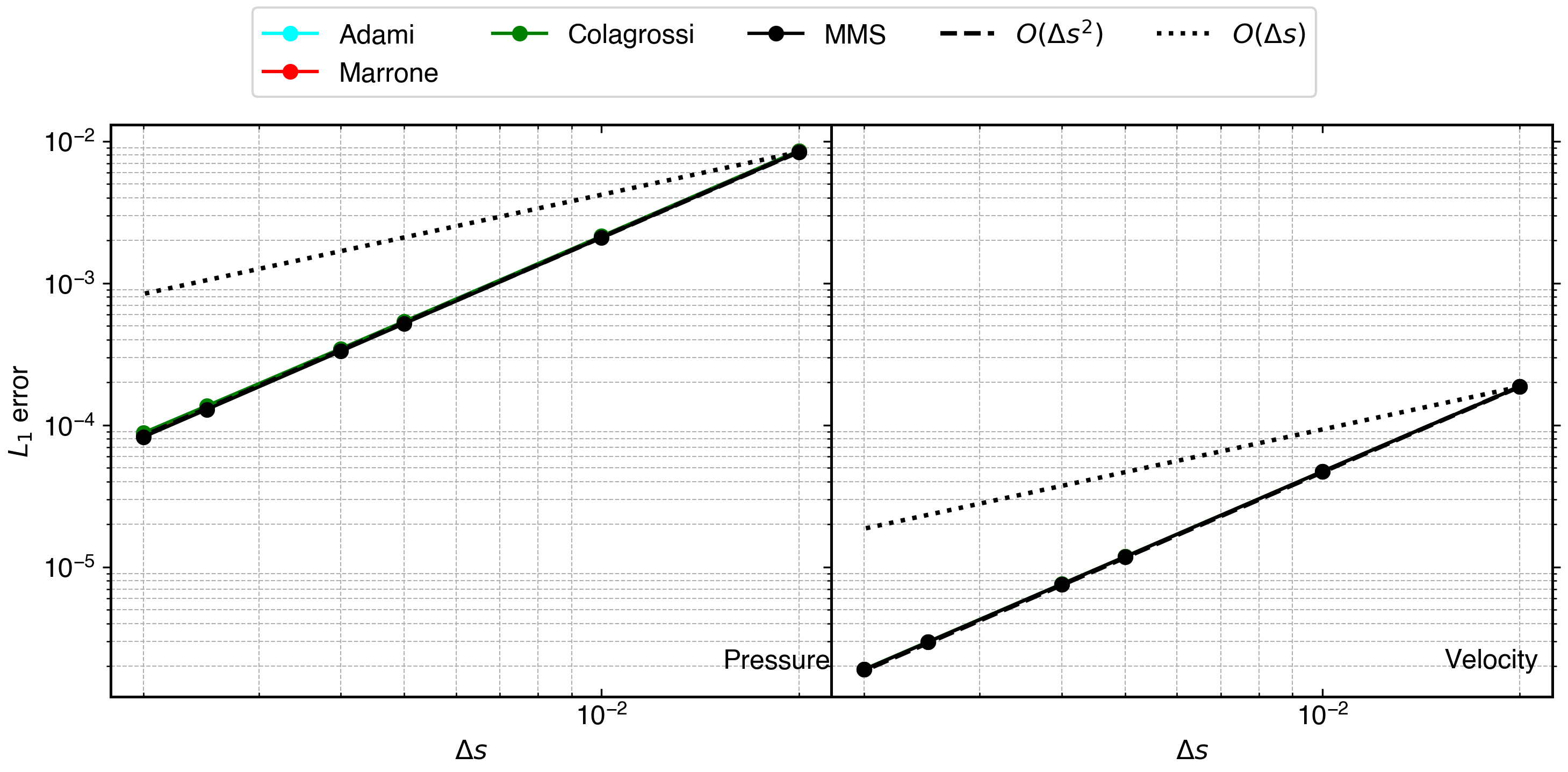
Figure 16: $L_{1}$ error in pressure and velocity after 100 time steps for different slip boundary implementations in straight domain as shown in fig. 9.

We construct the MS for convex and concave domains in eq. 25 that satisfies $\mathbf{u}\cdot\mathbf{n}=0$ at respective boundary surfaces of interest. In fig. 17 and fig. 18, we plot the $L_{1}$ error for pressure and velocity in convex and concave domains after 100 timesteps, respectively. Clearly, the method proposed by Colagrossi and Landrini [13] diverges for higher resolutions. The method proposed by Adami et al. [36] shows convergence rate close to 1.6 whereas the method by Marrone et al. [14] is very close to second-order convergence.

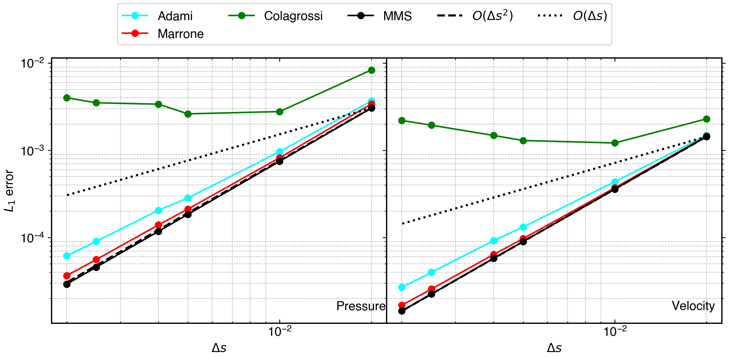
Figure 17: $L_{1}$ error in pressure and velocity after 100 time steps for different slip boundary implementations in the convex domain as shown in fig. 9.

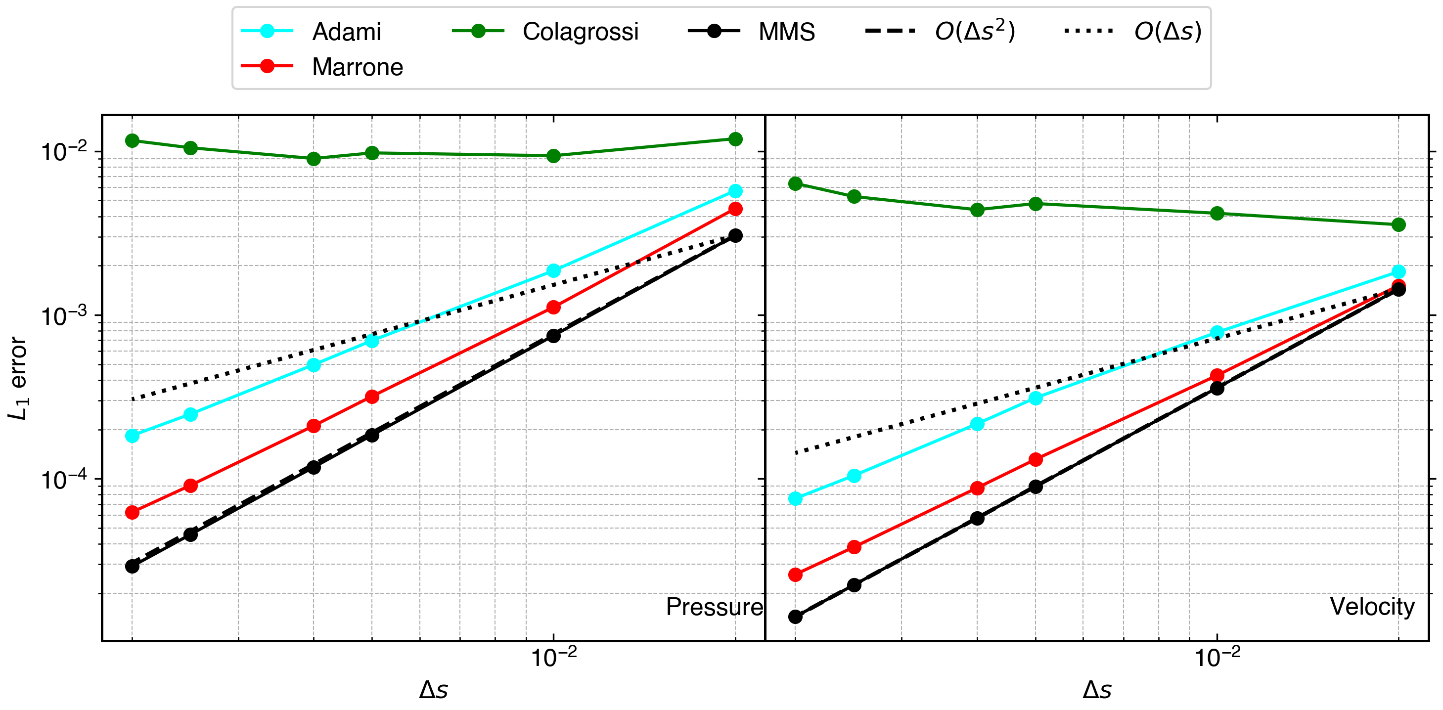
Figure 18: $L_{1}$ error in pressure and velocity after 100 time steps for different slip boundary implementations in the concave domain as shown in fig. 9.

We use the same MS for the packed-convex and packed-concave domains. In fig. 19 and fig. 20, we plot the $L_{1}$ error for pressure and velocity for packed-convex and packed-concave domains after 100 timesteps, respectively. As expected, The order of convergence is improved. In the packed domain, the convergence for the method by Adami et al. [36], and Marrone et al. [14] shows second order convergence. The method proposed by Colagrossi and Landrini [13] converges for lower resolutions in the case of the packed-convex domain but diverges in the case of packed-concave domain. This shows that mirroring the fluid particles for a curved surface does not result in a convergent boundary condition implementation.

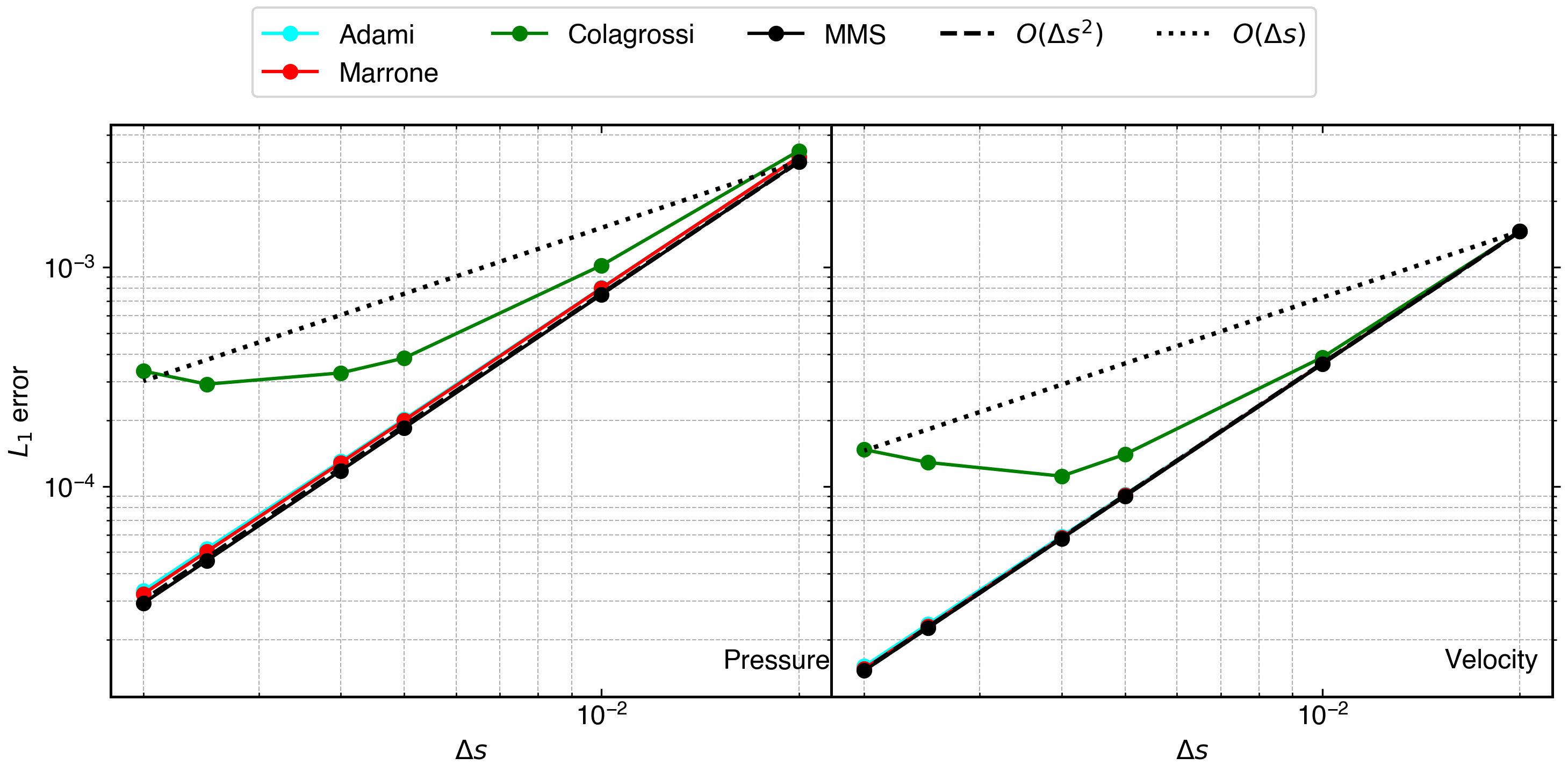
Figure 19: $L_{1}$ error in pressure and velocity after 100 time steps for different slip boundary implementations in the packed-convex domain as shown in fig. 10.

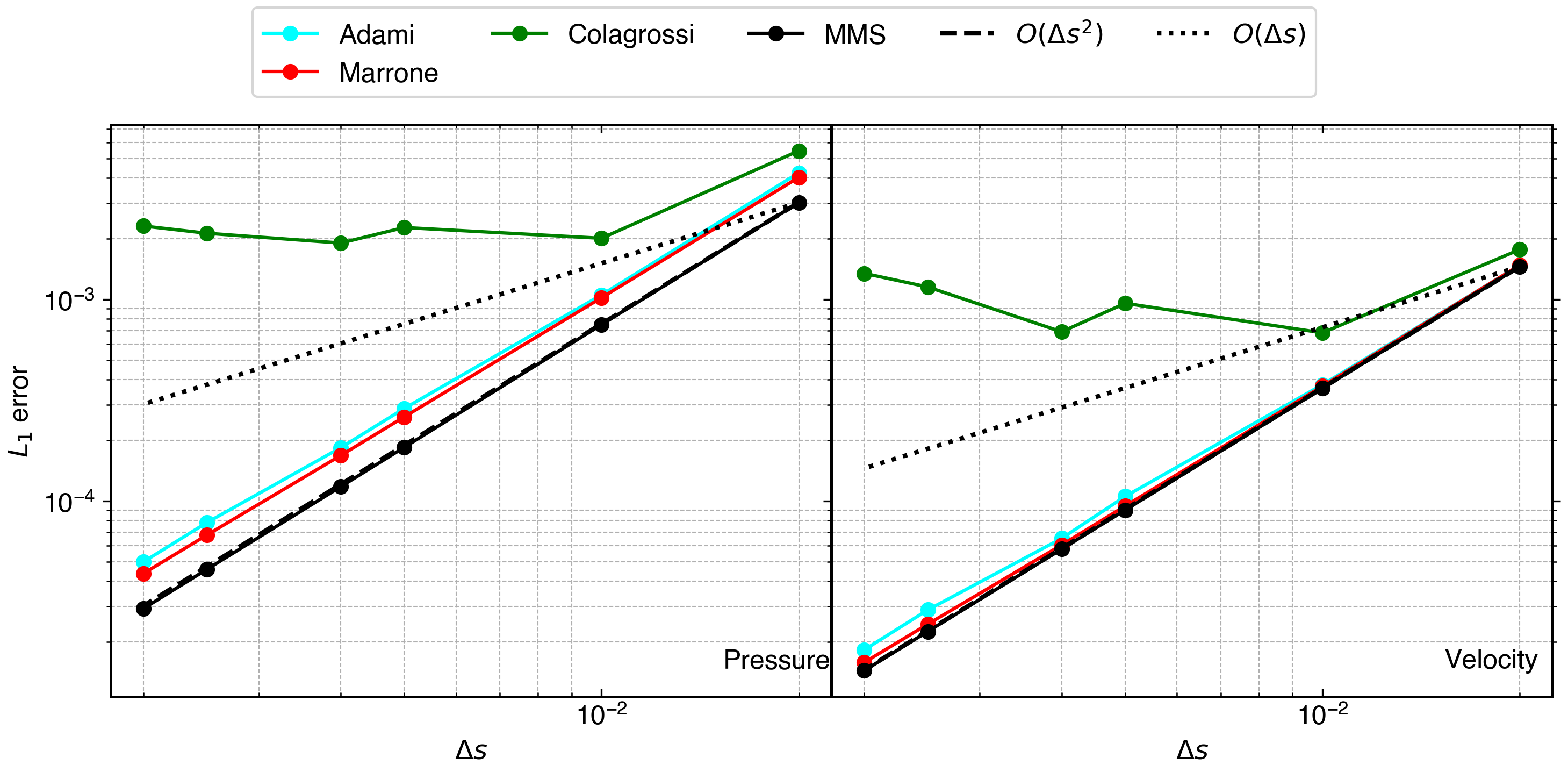
Figure 20: $L_{1}$ error in pressure and velocity after 100 time steps for different slip boundary implementations in the packed-concave domain as shown in fig. 10.

6.1.3 No-slip boundary condition

In this section, we test different no-slip boundary implementations discussed in section 3 using the domains used in the previous section. In all the no-slip boundary condition implementations, we apply no-penetration along with the no-slip boundary. In order to construct an MS for no-slip boundary condition, we satisfy $\mathbf{u}=0$ at the boundary. For the straight domain, we use the MS in eq. 26. In fig. 21, we plot the $L_{1}$ error for pressure and velocity in the domain after 100 timesteps. Clearly, all the methods show a convergence rate very close to second order.

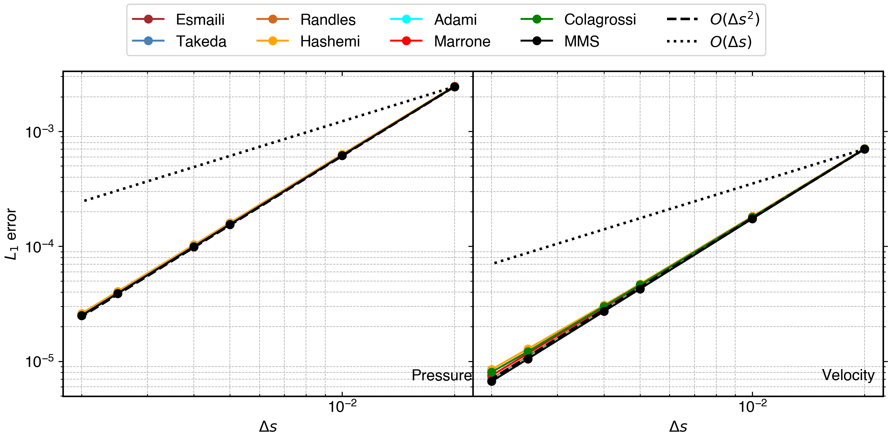
Figure 21: $L_{1}$ error in pressure and velocity after 100 time steps for different no-slip boundary implementations in the straight domain as shown in fig. 9.

Generally, we find that objects on which we intend to apply no-slip boundary are curved. Therefore, we simulate all the methods on the domains having curved surfaces. For the convex domain, we use the MS in eq. 27 whereas for concave domain, we use eq. 28. In fig. 22 and fig. 23, we plot the $L_{1}$ error in pressure and velocity for convex and concave domains, respectively. Clearly, the method proposed by Hashemi et al. [45] diverges for a curved surface. The errors in the solutions are more in the concave domain compared to the convex domain. The method by Randles and Libersky [12], Esmaili Sikarudi and Nikseresht [37], Adami et al. [36] shows first-order convergence. Whereas methods by Colagrossi and Landrini [13], and Marrone et al. [14] shows close to 1.5. Some methods like by Takeda et al. [10] cannot be applied on the jagged boundary as some particles may lie on the surface, which may result zero in the denominator of eq. 13.

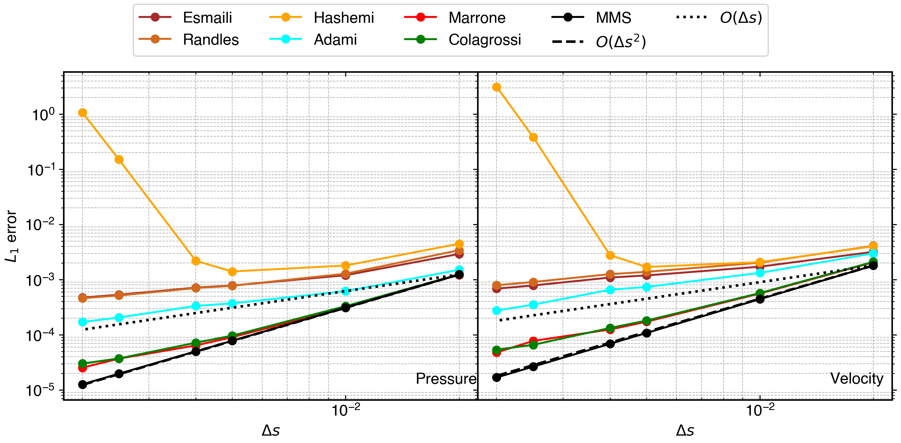
Figure 22: $L_{1}$ error in pressure and velocity after 100 time steps for different no-slip boundary implementations in the convex domain as shown in fig. 9.

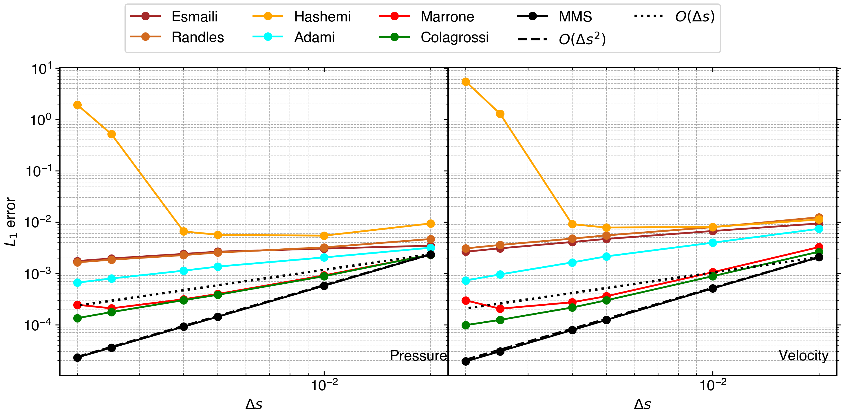
Figure 23: $L_{1}$ error in pressure and velocity after 100 time steps for different no-slip boundary implementations in the concave domain as shown in fig. 9.

Similar to other tests, we use the packed version of convex and concave domains to test the convergence of the methods on packed domains. We use the MS in eq. 27, and eq. 28 for the packed-convex and packed-concave domains, respectively. In the figure fig. 24, and fig. 25, we plot the $L_{1}$ error in pressure and velocity for packed-convex and packed-concave domains, respectively. As expected, the convergence is improved. The method by Adami et al. [36] does not show any convergence due to zero order interpolation used on the ghost particles. Method by Takeda et al. [10], Hashemi et al. [45], Randles and Libersky [12], Esmaili Sikarudi and Nikseresht [37] shows close to first order convergence. Clearly, the method by Marrone et al. [14] shows convergence close to the method when MS is used on the ghost particles. Further, the method of Colagrossi and Landrini [13] also shows good convergence, however the error compared to Marrone et al. [14] method is 2 order of magnitude higher. In the case of the packed-concave domain in fig. 25, the order of convergence shown by all methods is lower compared to packed-convex domain results.

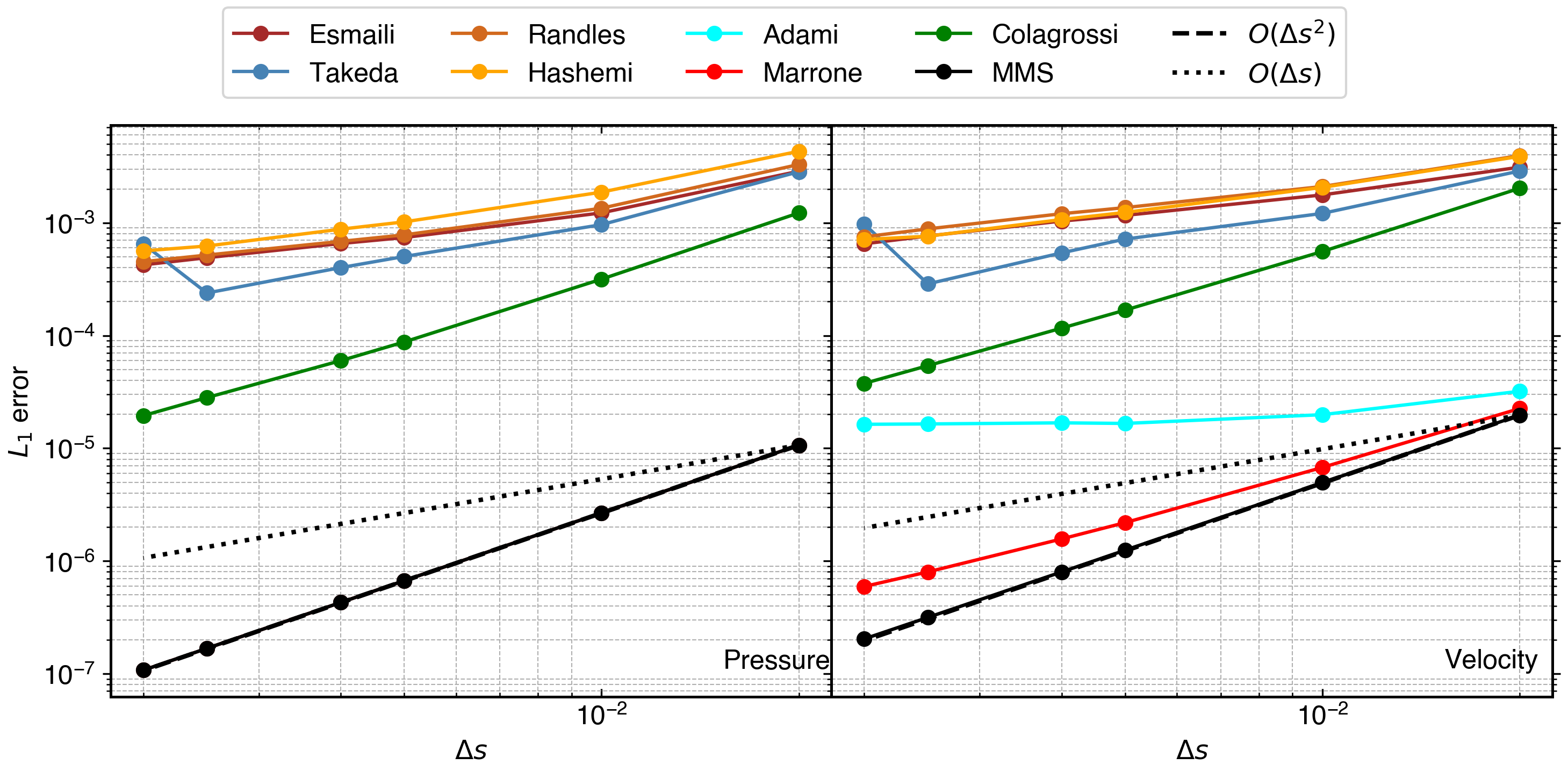
Figure 24: $L_{1}$ error in pressure and velocity after 100 time steps for different no-slip boundary implementations in the packed-convex domain as shown in fig. 10. Note that Marrone results overlaps the results of MMS.

Figure 25: $L_{1}$ error in pressure and velocity after 100 time steps for different no-slip boundary implementations in the packed-concave domain as shown in fig. 10. Note that Marrone results overlaps the results of MMS.

Method	Neumann Pressure	Slip	No-Slip
Adami [36]	($1.17\times 10^{-5}$)2.00	($1.82\times 10^{-5}$)1.95	($5.26\times 10^{-5}$)0.09
Colagrossi [13]	($1.18\times 10^{-5}$)2.00	($1.34\times 10^{-3}$)0.19	($7.47\times 10^{-5}$)1.52
Esmaili [37]	-	-	($2.54\times 10^{-3}$)0.55
Fourtakas [15]	($2.07\times 10^{-5}$)1.66	-	-
Hashemi [16]	($4.39\times 10^{-3}$)0.47	-	($2.11\times 10^{-3}$)0.72
Marongiu [32]	($1.14\times 10^{-3}$)0.63	-	-
Marrone [14]	($1.15\times 10^{-5}$)2.00	($1.58\times 10^{-5}$)1.97	($1.00\times 10^{-6}$)1.35
Randles [12]	-	-	($2.91\times 10^{-3}$)0.62
Takeda [10]	-	-	($8.63\times 10^{-4}$)0.86

Table 1: Table showing the summary of the error (in brackets) at the resolution $500\times 500$ and order of convergence of various boundary condition methods in the packed-concave domain.

In order to summarize the results, since the straight and convex domain shows better results compared to concave domain, we consider the results for a concave domain only. Furthermore, we compile results for a packed domain only since the packed domains are preferred over the unpacked ones. In the case of the no-slip and slip boundary, we focus on the convergence of velocity, and in the case of the Neumann pressure, we focus only on the convergence of pressure. In table 1, we tabulate the error at the highest resolution, i.e. $\Delta x=1/500$, and the approximate order of convergence for all the boundary conditions and methods. Clearly, in the case of the Neumann pressure boundary condition, Adami, Colagrossi, and Marrone converges well. In the case of the slip boundary conditon only the Adami and Marrone methods work. Whereas in the case of the no-slip boundary only Colagrossi and Marrone method show reasonable convergence. Clearly, Marrone method is able to reach lowest error as well as show convergence for all the types of boundary conditions.

6.2 Comparison of open boundary condition implementations

In this section, we test various inlet and outlet boundary condition implementations discussed in section 4. In order to test the boundary condition implementation, we require the inlet and outlet boundary to continuously add and remove particles from the domain, respectively. Furthermore, the inlet and outlet condition requires that the flow is only along the normal at the boundary. In order to satisfy these conditions, we use a $1m\times 1m$ domain, with an inlet and outlet on the left and right, respectively. In fig. 26, we show the domain with ghost particles representing the inflow (in green), outflow (in red), and wall (in orange). In the following sections, we discuss inlet boundary condition implementations first, followed by outlet boundaries.

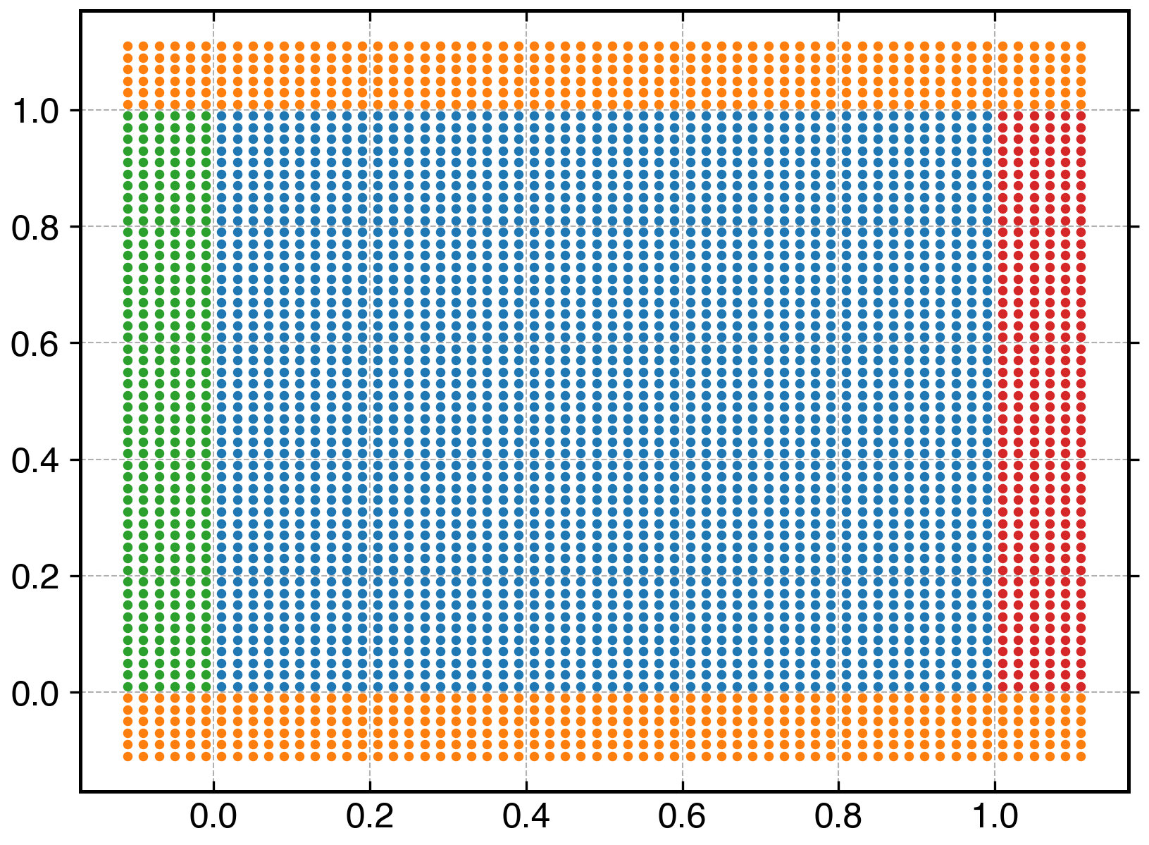
Figure 26: The domain used for the verification of inlet and outlet boundary implementation. The blue particles represent the fluid, orange particle represent the wall, green particles are inflow particles, and red particles are the outflow particles.

6.2.1 Inlet boundary

In order to test the inlet velocity boundary condition, we use the MS in eq. 29. In fig. 27, we plot the $L_{1}$ error in pressure and velocity after 100 timesteps for all the velocity inflow boundary implementations. We test all the methods discussed in section 4 viz. mirror, simple-mirror, and hybrid. We observe that both mirror and simple-mirror perform well for a velocity inlet boundary condition. Whereas the hybrid is bounded by the limiting error in both pressure and velocity.

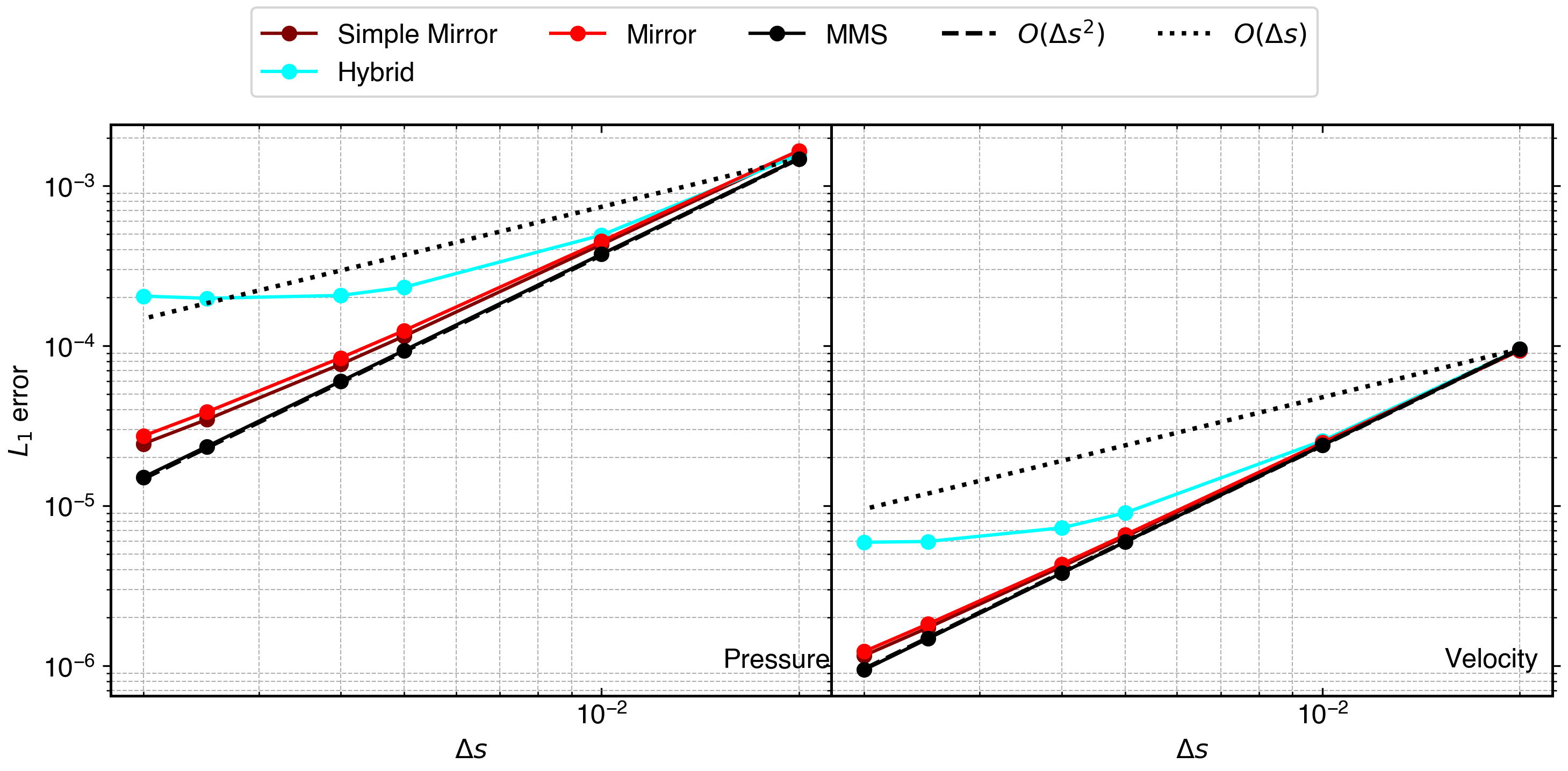
Figure 27: $L_{1}$ error in pressure and velocity after 100 time steps for different inlet velocity boundary implementations in the domain as shown in fig. 26.

In order to test the pressure inflow boundary implementation, we use the MS in eq. 32. In fig. 28, we plot the $L_{1}$ error in pressure and velocity after 100 timesteps for all the velocity inflow boundary implementations. Clearly, the boundary implementation for a pressure inflow boundary is second-order accurate for all the methods. In the case of the hybrid method, a slight deviation in the convergence can be seen.

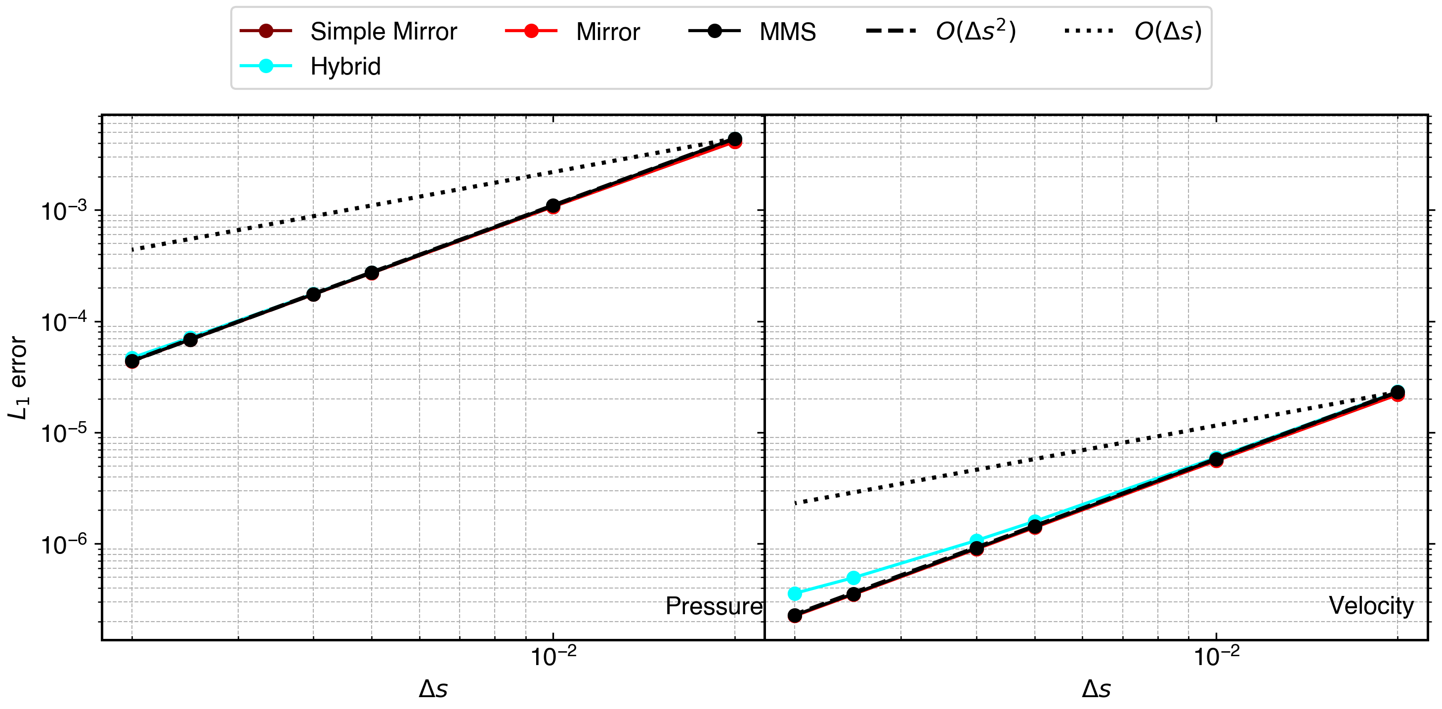
Figure 28: $L_{1}$ error in pressure and velocity after 100 time steps for different inlet pressure boundary implementations in the domain as shown in fig. 26.

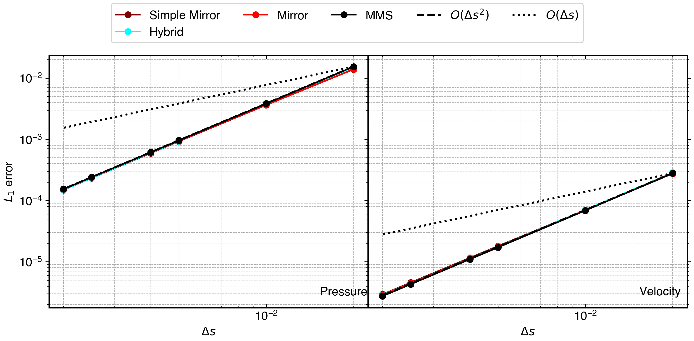
Figure 29: $L_{1}$ error in pressure and velocity after 500 time steps for different inlet velocity wave going upstream boundary implementations as shown in the domain in fig. 26.

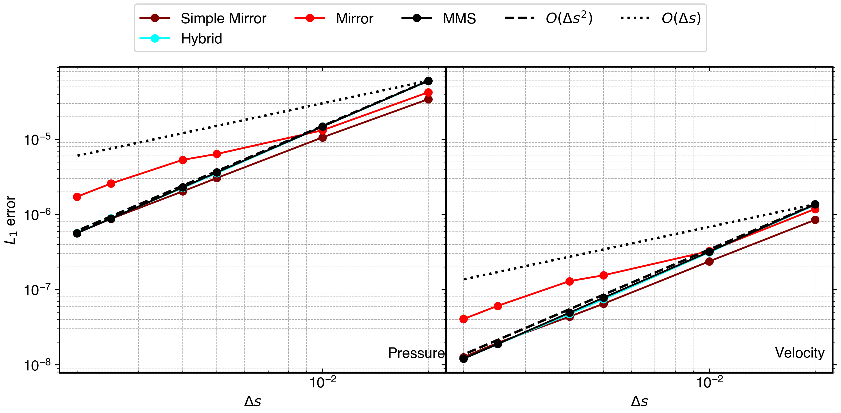
Figure 30: $L_{1}$ error in pressure and velocity after 500 time steps for different inlet pressure wave going upstream boundary implementations as shown in the domain in fig. 26.

Since in WCSPH, due to weakly compressible assumption, waves travel with a speed of artificial velocity of sound. We use the MS simulating a wave passing out of the inlet, these kind of waves are encountered when a jump start is performed on a wind tunnel kind of simulation. We simulate the problem for 500 iterations in order to allow the wave to completely pass through the inlet/outlet. We use the MS in eq. 30 for the inlet velocity wave. In fig. 29, we plot the $L_{1}$ error in pressure and velocity for all the methods. Clearly, the hybrid method also shows second-order convergence along with other methods.

In order to simulate a pressure wave going out of the inlet, we use the MS in eq. 33. In fig. 30, we plot the $L_{1}$ error in pressure and velocity for all the methods. The mirror method shows a slight increase in error for higher resolutions. The simple-mirror remains at the same level of error compared to the hybrid method, which shows second-order convergence.

6.2.2 Outlet boundary

The outflow is different compared to the inlet as we usually do not have any information about the ghost particles in these regions. In order to test the outflow velocity boundary condition, we use the MS in eq. 29. In fig. 31, we plot the $L_{1}$ error in pressure and velocity after 100 timesteps for all the velocity outflow boundary implementation. The do-nothing and the hybrid boundary are both bounded by a limiting error which is proportional to the speed of sound. As before, both mirror and simple-mirror show second-order convergence for velocity outlet boundary condition.

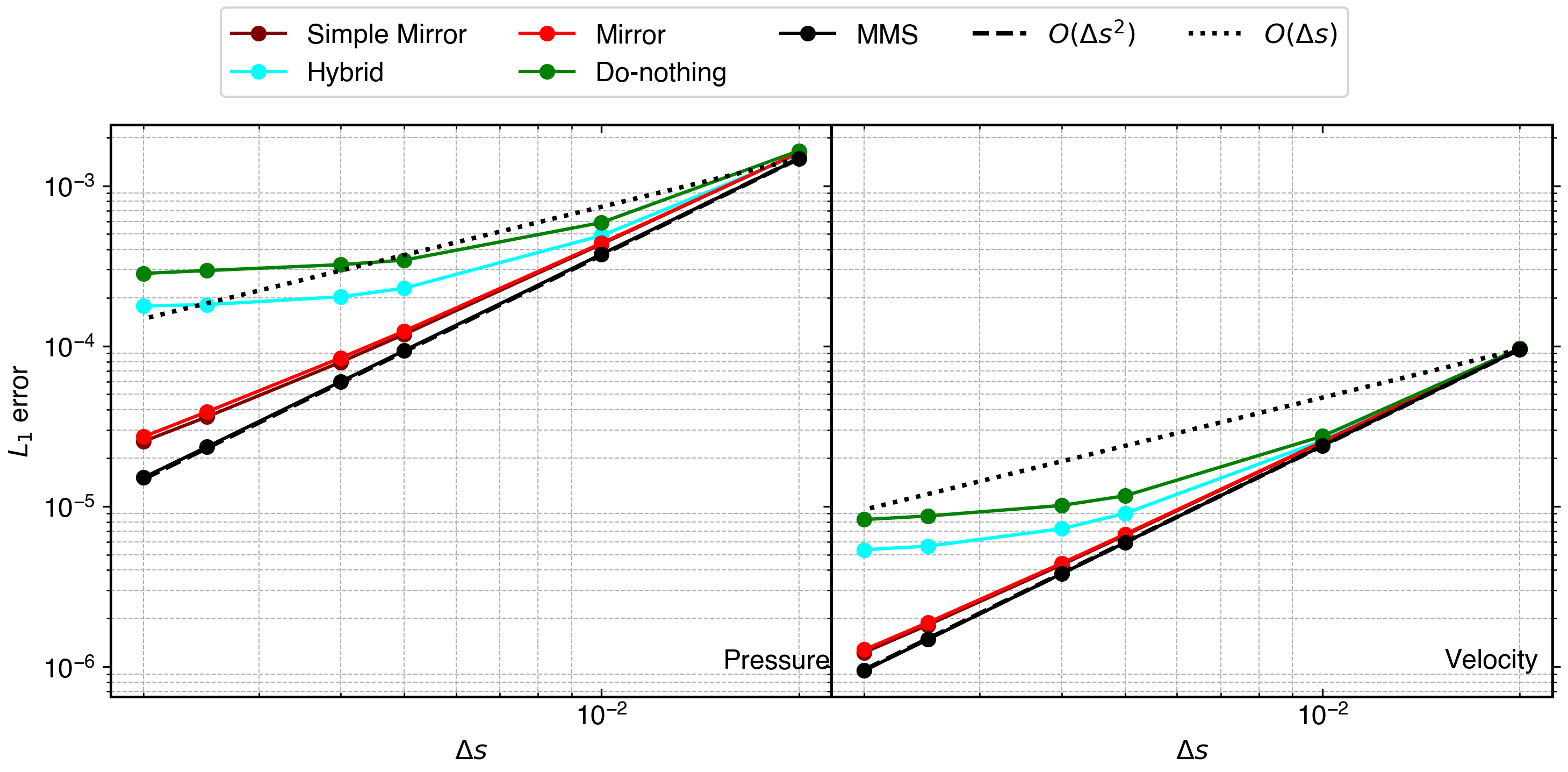
Figure 31: $L_{1}$ error in pressure and velocity after 100 time steps for different outlet velocity boundary implementations in the domain as shown in fig. 26.

In order to test the pressure outflow boundary implementation, we use the MS in eq. 32. In fig. 32, we plot the $L_{1}$ error in pressure and velocity after 100 timesteps for all the velocity outflow boundary implementation. Clearly, all the methods show second-order convergence.

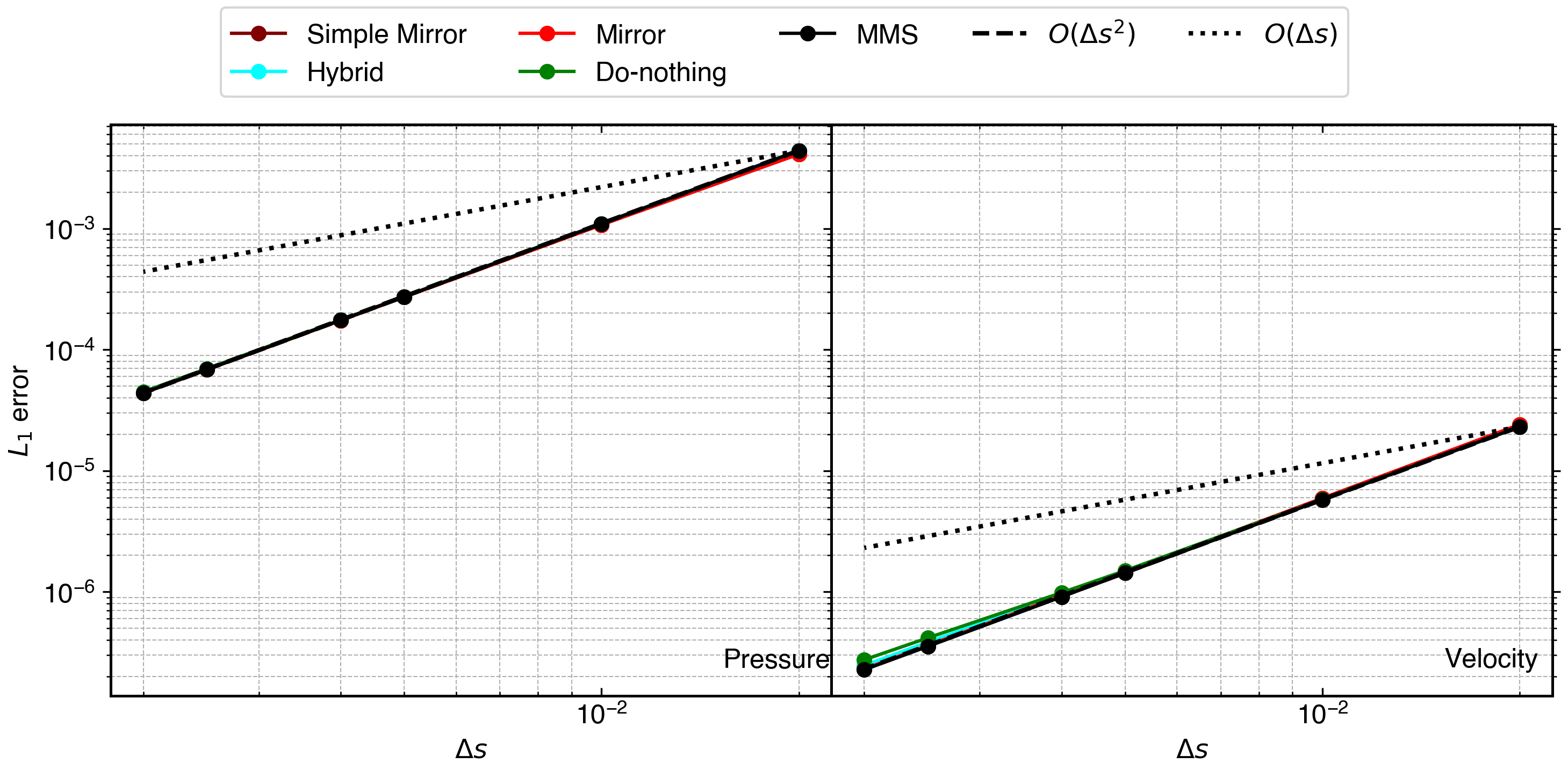
Figure 32: $L_{1}$ error in pressure and velocity after 100 time steps for different outlet pressure boundary implementations in the domain as shown in fig. 26.

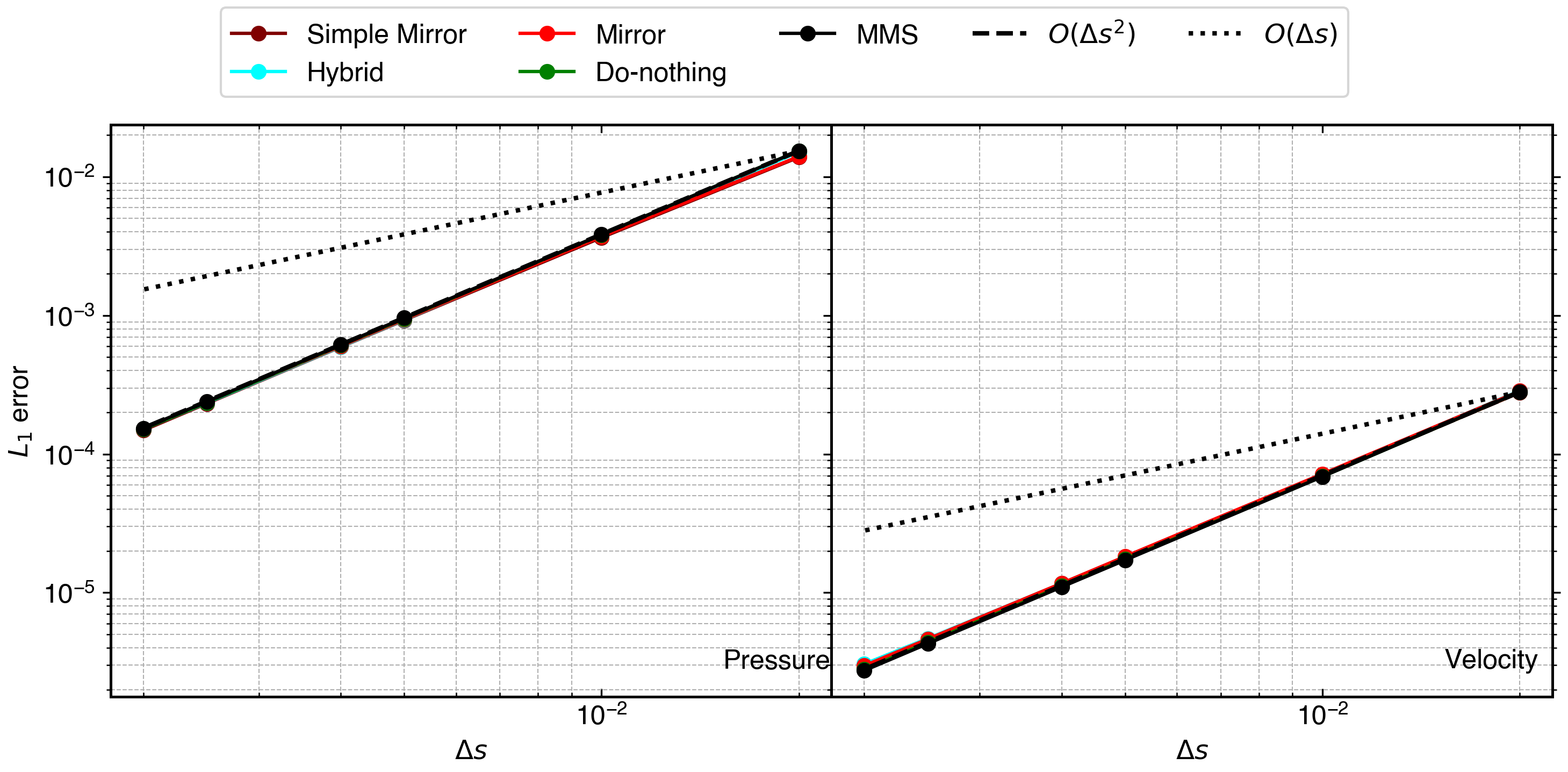
Figure 33: $L_{1}$ error in pressure and velocity after 500 time steps for different outlet velocity wave going downstream boundary implementations in the domain as shown in fig. 26.

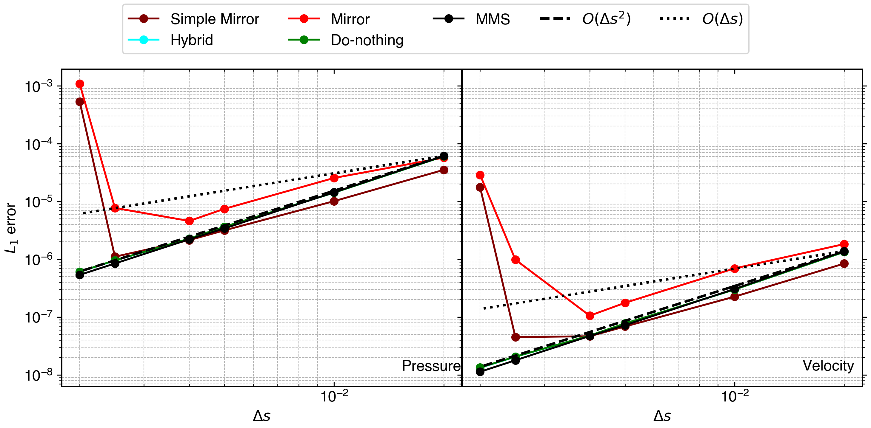
Figure 34: $L_{1}$ error in pressure and velocity after 500 time steps for different outlet pressure boundary wave going downstream implementations in the domain as shown in fig. 26.

To investigate the behavior of the outlet boundary implementation under the influence of a passing wave, we use the MS given in eq. 34 and eq. 31 for outlet pressure and outlet velocity boundary implementations, respectively. In fig. 33, and fig. 34, we plot the $L_{1}$ error for pressure and velocity after 500 timesteps for both the MS. In the case of the velocity wave, all the methods show second order convergence. However, in the case of the pressure wave in fig. 34, the mirror and simple-mirror method diverges. This shows that the mirror and simple-mirror methods are not truly non-reflecting and are unable to pass a pressure wave. These results support the finding of Negi and Ramachandran [7], where a short domain with the mirror outlet was found to be unstable.

Method	Velocity in	Pressure in
Hybrid[22]	$(2.87\times 10^{-6})$ 2.00	$(5.66\times 10^{-7})$ 2.02
Mirror[21]	$(2.84\times 10^{-6})$ 1.97	$(1.71\times 10^{-6})$ 1.38
Simple Mirror	$(2.93\times 10^{-6})$ 1.98	$(5.64\times 10^{-7})$ 1.81

Table 2: Summary of results for the wave traveling upstream out of the inlet for all the methods. Error at highest resolution is shown in brackets.

Method	Velocity out	Pressure out
Do-nothing[20]	$(2.80\times 10^{-6})$ 2.00	$(6.08\times 10^{-7})$ 2.00
Hybrid[22]	$(3.05\times 10^{-6})$ 1.99	$(6.05\times 10^{-7})$ 2.00
Mirror[21]	$(2.97\times 10^{-6})$ 1.97	$(1.01\times 10^{-3})$ -3.63
Simple Mirror	$(2.86\times 10^{-6})$ 1.97	$(5.34\times 10^{-4})$ -4.21

Table 3: Summary of results for the wave traveling downstream out of the outlet for all the methods. Error at highest resolution is shown in brackets.

In order to summarize the results for the open boundary conditions, we consider only the results for the traveling wave since, in WCSPH, it is important that the waves that are generated must be allowed to pass through inlet/outlet without affecting the flow. In case of a velocity wave, we focus on errors in velocity, whereas in the case of a pressure wave, we focus on errors in pressure. In table 2 and table 3, we tabulate the error for the highest resolution and the approximate order of convergence for all the methods simulating traveling wave MS. Clearly, the mirror method show significant decrease in order of convergence in the case of the pressure wave moving upstream. In case of the wave traveling downstream, both mirror and simple-mirror diverge. The hybrid method is applicable and converge for both the scenarios.

6.3 Performance Comparison

In this section, we compare the performance of three solid boundary condition implementations, viz. Marrone, Colagrossi, and Adami. For this testcase, we use a 10 core, dual socket Intel(R) Xeon(R) CPU E5-2650 v3 processor CPU. In the context of complexity, the Adami method requires only one loop over all the fluid particles to extrapolate properties from fluid, whereas the Colagrossi method requires the creation and deletion of particles in every timestep. In the case of the Marrone method, one needs to solve an additional $4\times 4$ matrix for each particle in the solid boundary, excluding the extrapolation step.

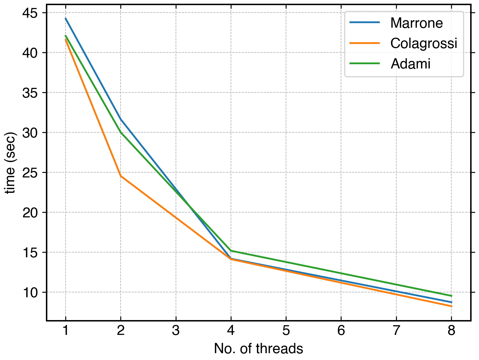
Figure 35: The time taken with the increase in the number of threads for different solid boundary conditions.

In fig. 35, we plot the time taken versus the no of parallel computing threads for 100 timesteps for a $100\times 100$ domain. Clearly, the time taken are very close despite the fact that different amount of computations are required. This is due to a very low number of solid particle compared to the fluid particles. In the present case, the fluid particles are $10000$, whereas the solid particles on which boundary condition is implemented are $600$. Therefore, we demonstrated that a higher order boundary implementation does not affect the performance of the solver. Furthermore, these results can be easily extrapolated to open-boundary implementations. In the next section, we propose an algorithm to obtain a convergent solver for a problem containing inlet, outlet, and solid boundaries.

7 Complete second order convergent SPH scheme

In the previous section, we have shown that some of the boundary condition implementations are convergent using the MMS. Recently, Negi and Ramachandran [26], and Negi and Ramachandran [7] have used verification methods to procedurally obtain a second order accurate WCSPH scheme without boundary as discussed in section 2. In this section, we extend their method to propose a second-order convergent scheme with second-order convergent boundary implementations. For brevity, we use short names to represent an equation in the algorithm. For example, EvaluateVelocityOnGhost(dest, sources) can be written formally as shown in algorithm 1.

for i in dest do

       $u_{i}=0$;

       for j in sources do

             $u_{i}=u_{i}+u_{j}\omega_{j}W_{ij}$;

            

      

Algorithm 1 Psuedo-code of equation EvaluateVelocityOnGhost.

In algorithm 1, $i$ is the loop index and $j$ is over all the neighbors of $i$^th element. We note that all the extrapolation/equation require a corrected kernel/gradient and is implied.

Considering a fluid domain, the inlet continuously feeding particles to the fluid, and the outlet continuously consuming particles from the fluid and an arbitrary shaped solid body. In algorithm 2, we show the algorithm for a convergent time-accurate WCSPH scheme to simulate the flow for a given initial condition. We denote all the fluid particles by $\mathscr{F}$, all solid particles by $\mathscr{S}$, and all inlet/outlet particles by $\mathscr{IO}$. All the virtual particles required for solid particles are denoted by $\mathscr{M(S)}$.

while $t<t_{final}$ do

       for i in $\mathscr{F}$ do

             EvaluatePressure(dest=i, sources=$\phi$);

            

      for i in $\mathscr{IO}$ do

             EvaluateVelocityOnInletOutlet(dest=i, sources=$\mathscr{F}$);

             EvaluatePressureOnInletOutlet(dest=i, sources=$\mathscr{F}$);

            

      for i in $M(\mathscr{S})$ do

             EvaluateVelocityOnGhost(dest=i, sources=$\mathscr{F}\cup\mathscr{IO}$);

             EvaluatePressureOnGhost(dest=i, sources=$\mathscr{F}\cup\mathscr{IO}$);

            

      for i in $\mathscr{S}$ do

             EvaluateSlipVelocityOnSolidFromGhost(dest=i, sources=$\phi$);

             EvaluateNoSlipVelocityOnSolidFromGhost(dest=i, sources=$\phi$);

             EvaluatePressureOnSolidFromGhost(dest=i, sources=$\phi$);

            

      for i in $\mathscr{F}\cup\mathscr{S}$ do

             ComputeVelocityGradient(dest=i, sources=$\mathscr{F}\cup\mathscr{IO}$);

             # use extrapolated no slip velocity for solid

             ComputeVelocityGradientSolid(dest=i, sources=$\mathscr{S}$);

            

      for i in $\mathscr{F}$ do

             ContinuityEquation(dest=i, sources=$\mathscr{F}\cup\mathscr{IO}$);

             # use extrapolated slip velocity for solid

             ContinuityEquationSolid(dest=i, sources=$\mathscr{S}$);

             PressureForces(dest=i, sources=$\mathscr{F}\cup\mathscr{S}\cup\mathscr{IO}$);

             ComputeViscousForces(dest=i, sources=$\mathscr{F}\cup\mathscr{IO}$);

            

      for i in $\mathscr{F}\cup\mathscr{IO}$ do

             Integrate(dest=i, sources=$\phi$)

      

Algorithm 2 A Second order convergent scheme.

The algorithm starts with the evaluation of pressure from the equation of state given by eq. 2 in EvaluatePressure. In the next step, we evaluate pressure and velocity on inlet and outlet domain using the hybrid method [22] in EvaluatePressureOnInletOutlet, and EvaluateVelocityOnInletOutlet, respectively. We note that the inlet and outlet properties are updated, and then these are used as the source for solid properties in case of overlaps. We use the method by Marrone et al. [14] to evaluate properties on solid particles. We first evaluate first order accurate values on virtual particles in EvaluateVelocityOnGhost, and EvaluatePressureOnGhost and then use these values to obtain pressure, slip, and no-slip velocities in EvaluatePressureOnSolidFromGhost, EvaluateSlipVelocityOnSolidFromGhost, EvaluateNoSlipVelocityOnSolidFromGhost, respectively. In order to obtain second-order accurate viscous operator, we require velocity gradient on each particle, which is computed in ComputeVelocityGradient, and ComputeVelocityGradientSolid. We note that we consider no-slip extrapolated velocity for gradient computation. Finally, we evaluate accelerations due to various forces in ContinuityEquation, ContinuityEquationSolid, PressureForces, ComputeViscousForces. We note that, in the evaluation of the continuity equation, we use extrapolated slip velocity on solids [46]. We use the computed and extrapolated properties to integrate the particle properties and position. We use IPST to make the particles more uniform and update the properties using a first-order accurate correction. The IPST can be performed after every few timesteps. In our simulations, we perform shifting after every 10 iterations.

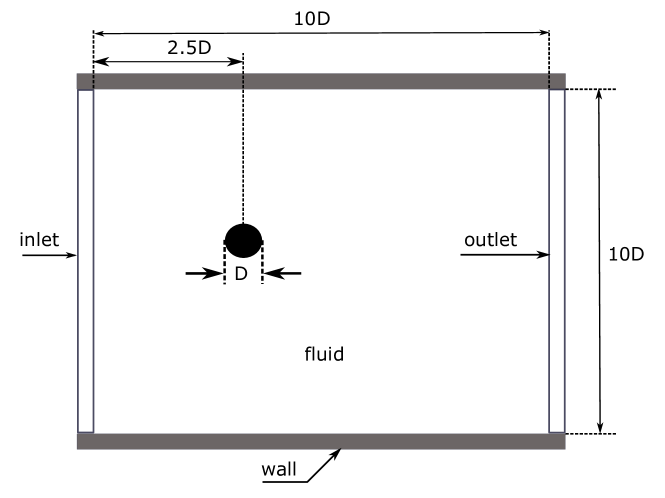
Figure 36: Description of the domain of the flow fast cylinder problem.

In order to show the accuracy achieved by the proposed algorithm, we solve the flow past a circular cylinder. We consider the domain shown in fig. 36. We consider inflow velocity $U=1m/s$, Reynolds number $Re=200$, and a cylinder of diameter $D=2m$. We set the dynamic viscosity $\nu=UD/Re$. We discretize the domain with $\Delta x=D/40$. The total particles in the domain are approximately $0.18M$. We simulate the problem using the algorithm 2 with artificial speed of sound $c_{o}=10m/s$ for $200sec$. We set the initial pressure $p_{o}=\rho c_{o}^{2}$, density $\rho_{o}=1.0$, and velocity $\mathbf{u}_{o}=U\hat{i}$. We add an additional density damping proposed by Antuono et al. [47] to the continuity equation with $\delta=0.0625$, to reduce high-frequency pressure oscillations (see the variations of SOC schemes proposed in sec. II.F of [7]).

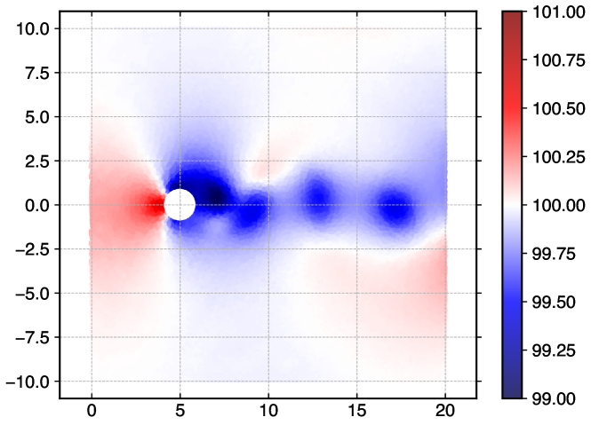
Figure 37: Average pressure at $t=100sec$.

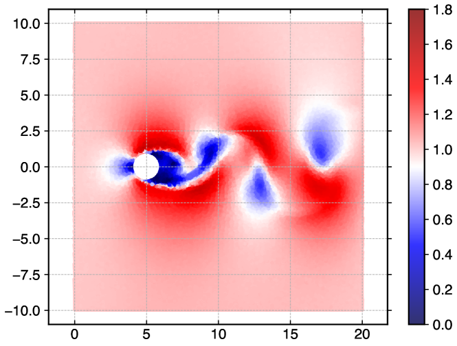
Figure 38: Velocity magnitude at $t=100sec$.

In fig. 37 and fig. 38, we plot the average pressure and velocity magnitude at $t=100sec$, respectively. We compute the average pressure $(p_{avg})_{i}=\sum p_{j}/N$, where the sum is taken over all the $N$ neighbors of the $i$^th particle. Cleary, the solution is free from any high frequency pressure oscillations. Futhermore, the pressure in the domain remains in the vicinity of the reference pressure $\rho c_{o}^{2}=100Pa$ for the entire simulation. We also compute the coefficient of lift $c_{l}$ and drag $c_{d}$ for the cylinder using the method proposed in Negi et al. [22].

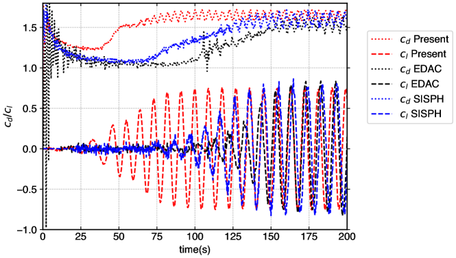
Figure 39: $c_{d}$ and $c_{l}$ variation for the flow past a cylinder with time.

In fig. 39, we plot the variation of $c_{d}$ and $c_{l}$ with time for the present method with results of Negi et al. [22] referred to as ”EDAC” and Muta et al. [46] referred to as ”SISPH”. We obtain the mean $c_{d}$ value of $1.65$ and $c_{l}$ value of $0.74$, after the shedding is established. These values are closer to SISPH values, where a pressure Poisson equation is solved to obtain pressure. Futhermore, both the drag and lift coefficient values are free from disturbances.

8 Conclusions

The convergence of the boundary condition implementations is a grand challenge[8] in SPH. In order to obtain a convergent boundary implementation, we require a scheme that must be convergent and should have the order of error lower than that in the boundary implementation. In this paper, we use the second order convergent scheme proposed by Negi and Ramachandran [7] to verify various boundary condition implementations. We use the MMS and construct MS for specific boundary conditions and domains. For a solid boundary, we verify methods for Neumann pressure, slip, and no-slip boundary conditions. In order to cover all the aspects of arbitrary geometries, we test the convergence on a straight, convex, and concave boundary. In the case of open boundaries, we consider a square domain with inlet and outlet regions simulating a wind-tunnel. We manufactured solutions for inlets and outlets for both Neumann pressure and velocity. Additionally, we manufactured solutions depicting waves of pressure and velocity passing through inlet/outlets.

We show that the method proposed by Marrone et al. [14] is convergent for all kinds of the domain and boundary conditions on a solid boundary. Some other method like Adami et al. [36], Colagrossi and Landrini [13] are second-order convergent in inviscid flow and packed domains. Almost all boundary implementations are second-order on a straight boundary. In the case of open boundaries, the mirror and simple-mirror work well in the absence of a wave traveling through the boundary. The hybrid and do-nothing boundaries are bounded by the $O(M^{2})$, where $M$ is the Mach number of the flow. However, in the case of a wave traveling through the domain, the mirror and simple-mirror method diverges, and hybrid and do-nothing methods converge with second-order accuracy. Finally, we discuss an algorithm to apply these boundary conditions in order to get a convergent solver. We use the method proposed by Marrone et al. [14] for solids and Negi et al. [22] for inlet and outlet boundaries. We demonstrate the accuracy of the proposed algorithm by solving the flow past a circular cylinder. We achieved the accuracy close to the results obtained using incompressible SPH solvers.

The manufactured solutions created in this paper can be used for any meshless solver for the specified domains. In this paper, we carried out appropriately 834 simulations, which take around 70 hours, which demonstrates the efficiency of the MMS. In the future, we would like to use the MMS to obtain a second-order convergent adaptive solver. Since the second-order convergence comes at the cost of performing kernel correction, the adaptivity in space and time will compensate for this and will result in a convergent and fast WCSPH solver.

We believe that with the identification of convergent boundary conditions along with second order convergent SPH schemes, it should be possible to build accurate and general purpose SPH-based solvers for the simulation of a wide variety of incompressible and weakly compressible fluid flow simulations. The recent advancements in adaptive resolution in SPH, will also facilitate the efficient simulation of such problems. In the future, we would like to use MMS to obtain a second-order convergent free surface boundary condition which are used widely in fluid and structure applications.

Appendix A Manufactured solutions

A.1 Neumann pressure boundary

In this boundary condition, we ensure that $\nabla p\cdot\mathbf{n}=0$, where $\mathbf{n}$ is normal to the boundary surface. For the straight domain the normal $\mathbf{n}=\mathbf{j}$, therefore, we can construct the MS given by,

$$\begin{split}u(x,y)&=\left(y-1\right)\sin{\left(2\pi x\right)}\cos{\left(2\pi y\right)}\\ v(x,y)&=-\left(y-1\right)\sin{\left(2\pi y\right)}\cos{\left(2\pi x\right)}\\ p(x,y)&=x^{2}+\cos{\left(4\pi x\right)}.\end{split}$$ (22)

In fig. 40, we show the contour plot of the above MS in straight domain.

Figure 40: Velocity and pressure contours on the straight domain in fig. 9 of the MS in eq. 22.

In the case of the convex domain, the normal to the surface is given by $\mathbf{n}=(x-0.5)\mathbf{i}+(y-0.5)\mathbf{j}$, therefore we can construct a MS is given by

$$\begin{split}u(x,y)&=\left(y-1\right)\sin{\left(2\pi x\right)}\cos{\left(2\pi y\right)}\\ v(x,y)&=-\left(y-1\right)\sin{\left(2\pi y\right)}\cos{\left(2\pi x\right)}\\ p(x,y)&=\tan^{-1}\left(\frac{(y-0.5)^{2}}{(x-0.5)^{2}}\right)\end{split}$$ (23)

In fig. 41, we show the contour plot of the above MS in the convex domain.

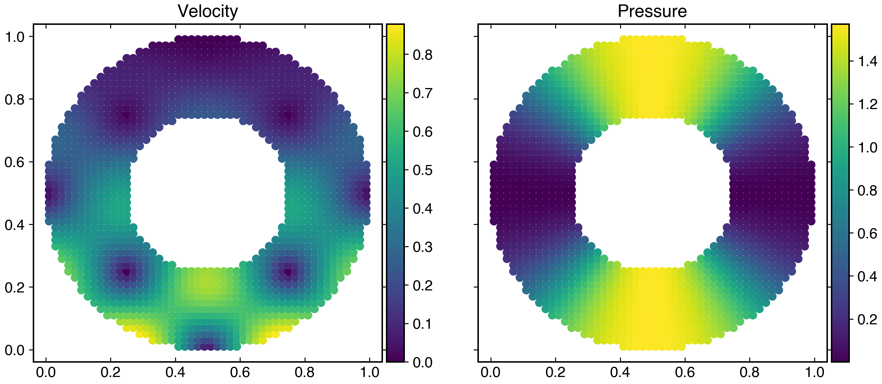
Figure 41: Velocity and pressure contours on the convex/concave domain of the MS in eq. 23.

Since, for the concave domain, the normal remains the same, we can use the same MS since it satisfies $\nabla p\cdot\mathbf{n}=0$ at the surface of interest. We note that for the packed version of the domain in fig. 10, we can use the same MS as used in the unpacked version as the surface of interest is exactly the same.

A.2 Slip boundary condition

For the slip boundary condition, we ensure that $\mathbf{u}\cdot\mathbf{n}=0$ at the boundary surface. For the straight domain, we construct the MS given by

$$\begin{split}u(x,y)&=\left(y-1\right)\sin{\left(2\pi x\right)}\cos{\left(2\pi y\right)}+1\\ v(x,y)&=\left(\left(y-1\right)^{2}\right)\sin{\left(2\pi y\right)}\\ p(x,y)&=\cos{\left(4\pi x\right)}+\cos{\left(4\pi y\right)}\\ \end{split}$$ (24)

In fig. 42, we plot the velocity and pressure contour generated by the MS in eq. 24.

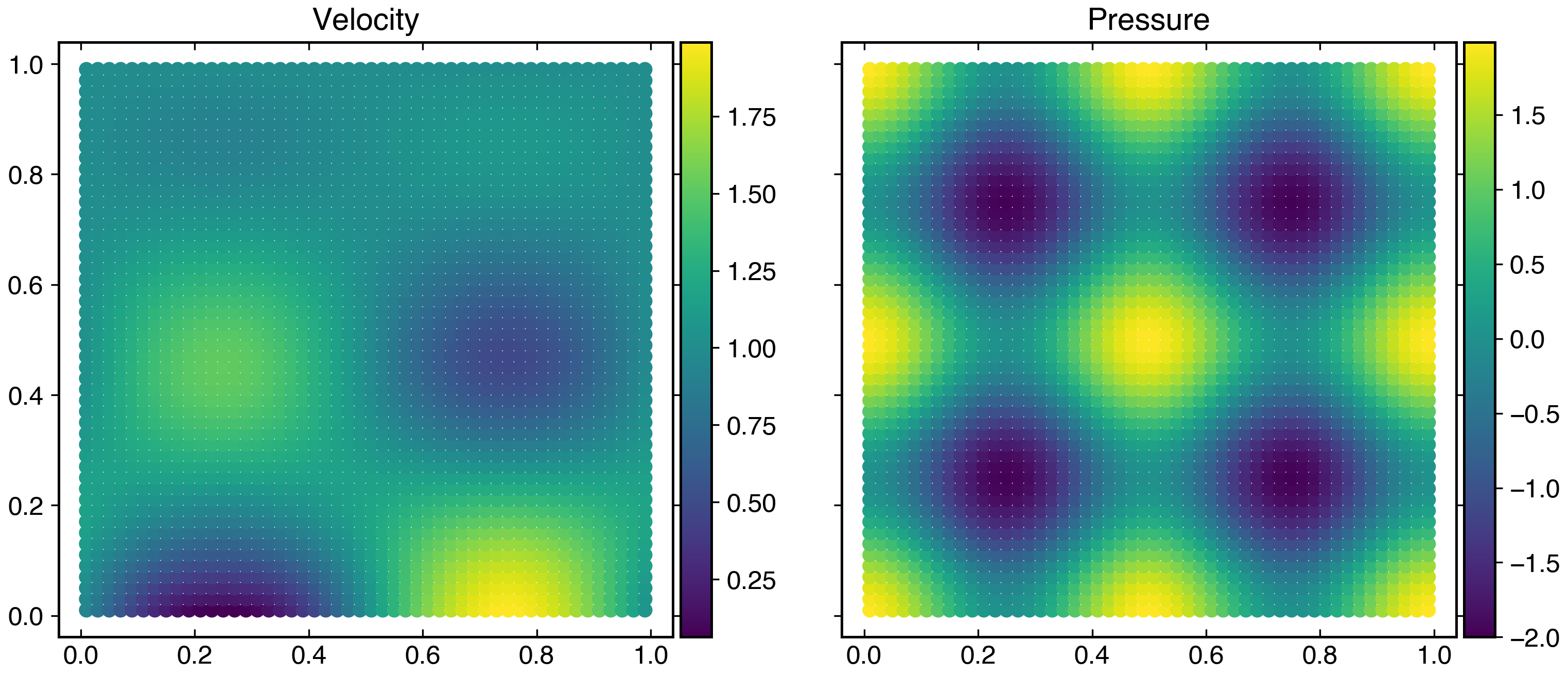
Figure 42: Velocity and pressure contours on the straight domain of the MS in eq. 24.

For the convex domain the normal $\mathbf{n}=(x-0.5)\mathbf{i}+(y-0.5)\mathbf{j}$, therefore we construct the MS given by

$$\begin{split}u(x,y)&=\left(y-0.5\right)\sin{\left(2\pi x\right)}\cos{\left(2\pi y\right)}\\ v(x,y)&=-\left(x-0.5\right)\sin{\left(2\pi x\right)}\cos{\left(2\pi y\right)}\\ p(x,y)&=\cos{\left(4\pi x\right)}+\cos{\left(4\pi y\right)}\\ \end{split}$$ (25)

such that $\mathbf{u}\cdot\mathbf{n}=0$. In fig. 43, we plot the velocity and pressure contour generated from the MS in eq. 24. We note that since for the concave as well as packed domains, the normal remains the same therefore we can use the same MS in eq. 25 for all these domains.

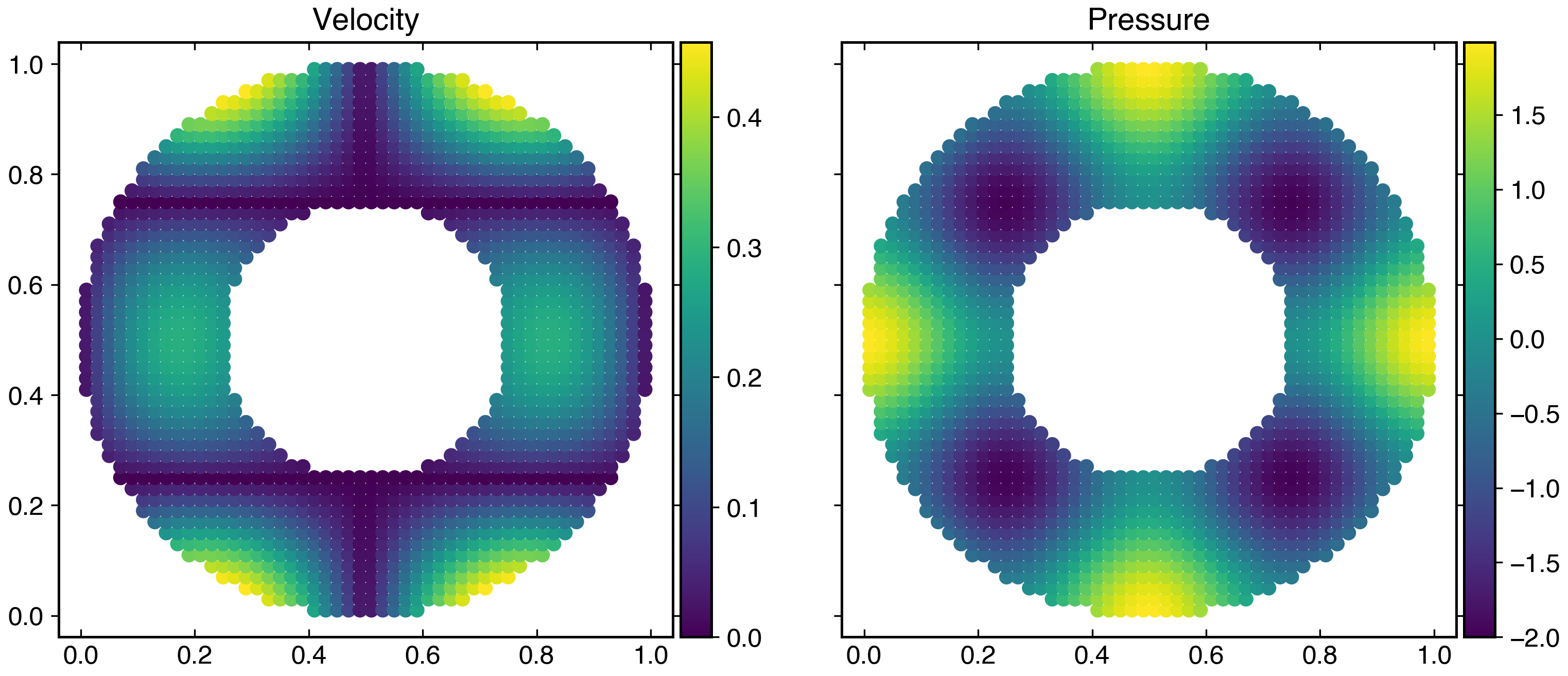
Figure 43: Velocity and pressure contours on the convex/concave domain of the MS in eq. 25.

A.3 No-slip boundary condition

For a no-slip boundary condition, we ensure that the velocity at the surface is zero for a stationary wall. For the straight domain, we construct the MS given by

$$\begin{split}u(x,y,t)&=\left(1-y\right)^{2}e^{-10t}\sin{\left(2\pi x\right)}\cos{\left(2\pi y\right)}\\ v(x,y,t)&=-\left(1-y\right)^{2}e^{-10t}\sin{\left(2\pi y\right)}\cos{\left(2\pi x\right)}\\ p(x,y,t)&=\left(\cos{\left(4\pi x\right)}+\cos{\left(4\pi y\right)}\right)e^{-10t}\end{split}$$ (26)

In fig. 44, we plot the contour plot for the velocity and pressure generated by the MS in eq. 26.

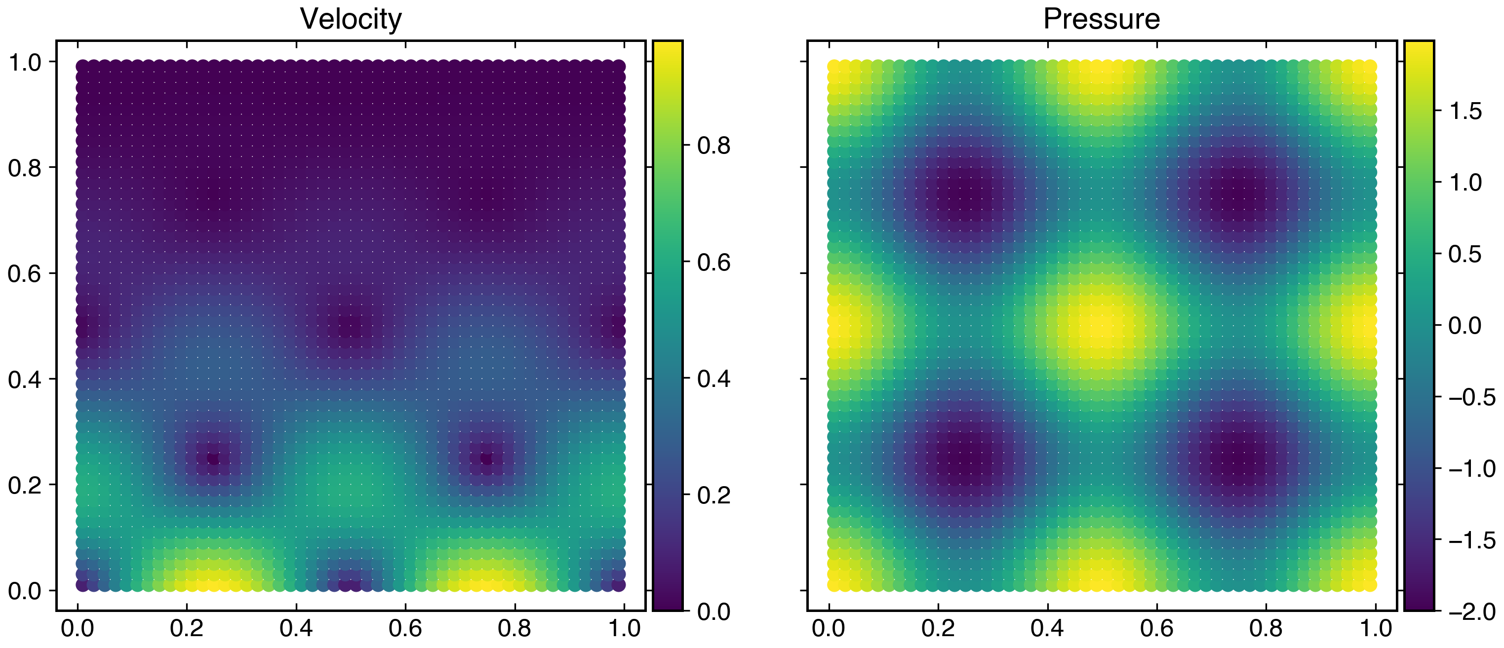
Figure 44: Velocity and pressure contours on the straight domain of the MS in eq. 26.

In order to construct an MS for the convex domain in fig. 9, we construct the MS such that the velocity is zero on the inner surface of the domain, given by

$$\begin{split}u(x,y,t)&=\left(-\left(x-0.5\right)^{2}-\left(y-0.5\right)^{2}+0.0625\right)\\ &e^{-10t}\sin{\left(\pi\left(2\left(x-0.5\right)^{2}+2\left(y-0.5\right)^{2}\right)\right)}\\ v(x,y,t)&=-\left(-\left(x-0.5\right)^{2}-\left(y-0.5\right)^{2}+0.0625\right)\\ &e^{-10t}\cos{\left(\pi\left(2\left(x-0.5\right)^{2}+2\left(y-0.5\right)^{2}\right)\right)}\\ p(x,y,t)&=\left(\cos{\left(4\pi x\right)}+\cos{\left(4\pi y\right)}\right)e^{-10t}\end{split}$$ (27)

In fig. 45, we plot the velocity and pressure contour generated from the MS in eq. 27.

Figure 45: Velocity and pressure contours on the convex domain of the MS in eq. 27.

In order to construct the MS for the concave domain in fig. 9, we make the velocity zero on the outer surfaces given by

$$\begin{split}u(x,y,t)&=\left(-\left(x-0.5\right)^{2}-\left(y-0.5\right)^{2}+0.25\right)\\ &e^{-10t}\sin{\left(\pi\left(2\left(x-0.5\right)^{2}+2\left(y-0.5\right)^{2}\right)\right)}\\ v(x,y,t)&=-\left(-\left(x-0.5\right)^{2}-\left(y-0.5\right)^{2}+0.25\right)\\ &e^{-10t}\cos{\left(\pi\left(2\left(x-0.5\right)^{2}+2\left(y-0.5\right)^{2}\right)\right)}\\ p(x,y,t)&=\left(\cos{\left(4\pi x\right)}+\cos{\left(4\pi y\right)}\right)e^{-10t}\end{split}$$ (28)

In fig. 46, we plot the contour for velocity and pressure generated from the eq. 28 for the concave domain. We note that the MS described remains the same for the corresponding packed version of the domains.

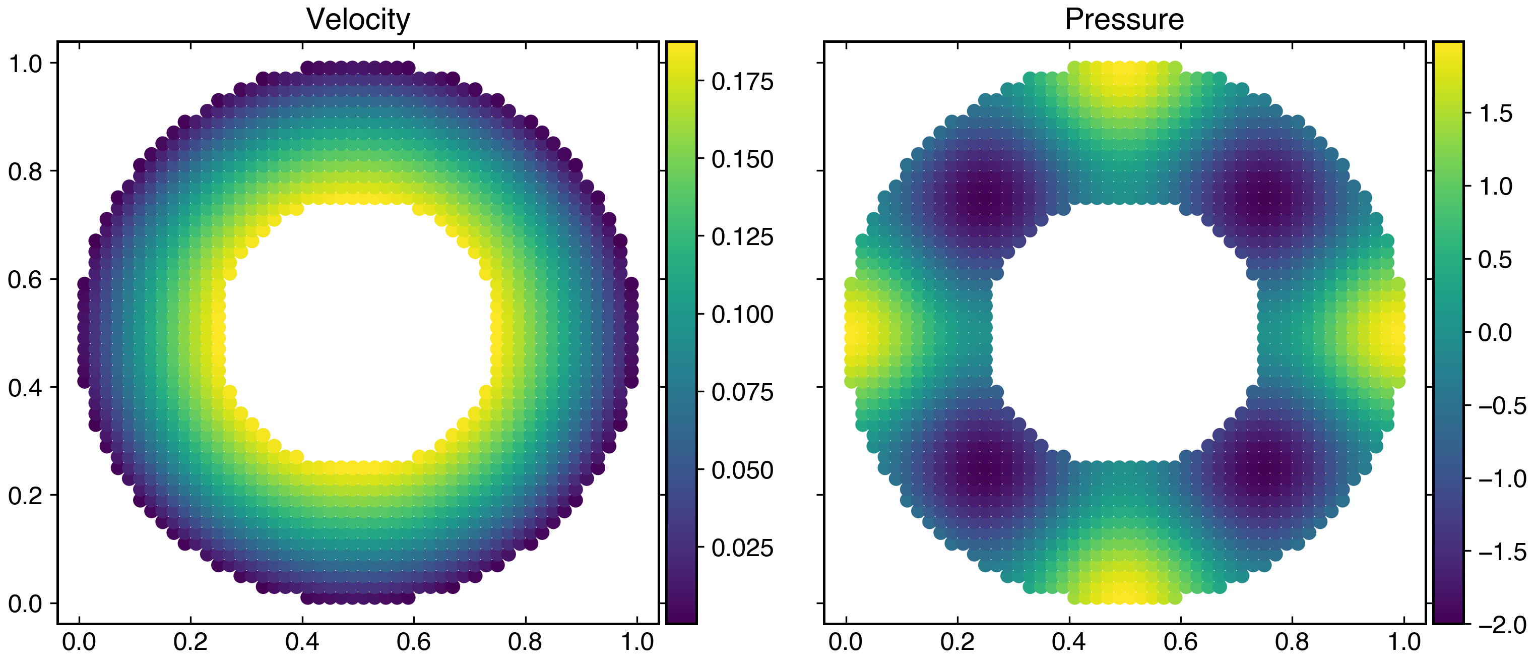
Figure 46: Velocity and pressure contours on the concave domain of the MS in eq. 28.

A.4 Inlet and outlet velocity boundary

At the inlet, we make sure that $\nabla\mathbf{u}\cdot\mathbf{n}=0$.‘’ Since the inlet is usually straight. We consider one type of inlet with constant normal $\mathbf{n}=-\mathbf{i}$ similarly outlet with normal $\mathbf{n}=\mathbf{i}$. We use the MS given by

$$\begin{split}u(x,y,t)&=y\left(y-1\right)e^{-10t}\cos{\left(2\pi y\right)}+1\\ v(x,y,t)&=-x^{2}\left(x-1\right)^{2}e^{-10t}\sin{\left(2\pi y\right)}\\ p(x,y,t)&=\left(\cos{\left(4\pi x\right)}+\cos{\left(4\pi y\right)}\right)e^{-10t}\end{split}$$ (29)

In the fig. 47, we plot the velocity and pressure contour for the MS in eq. 29.

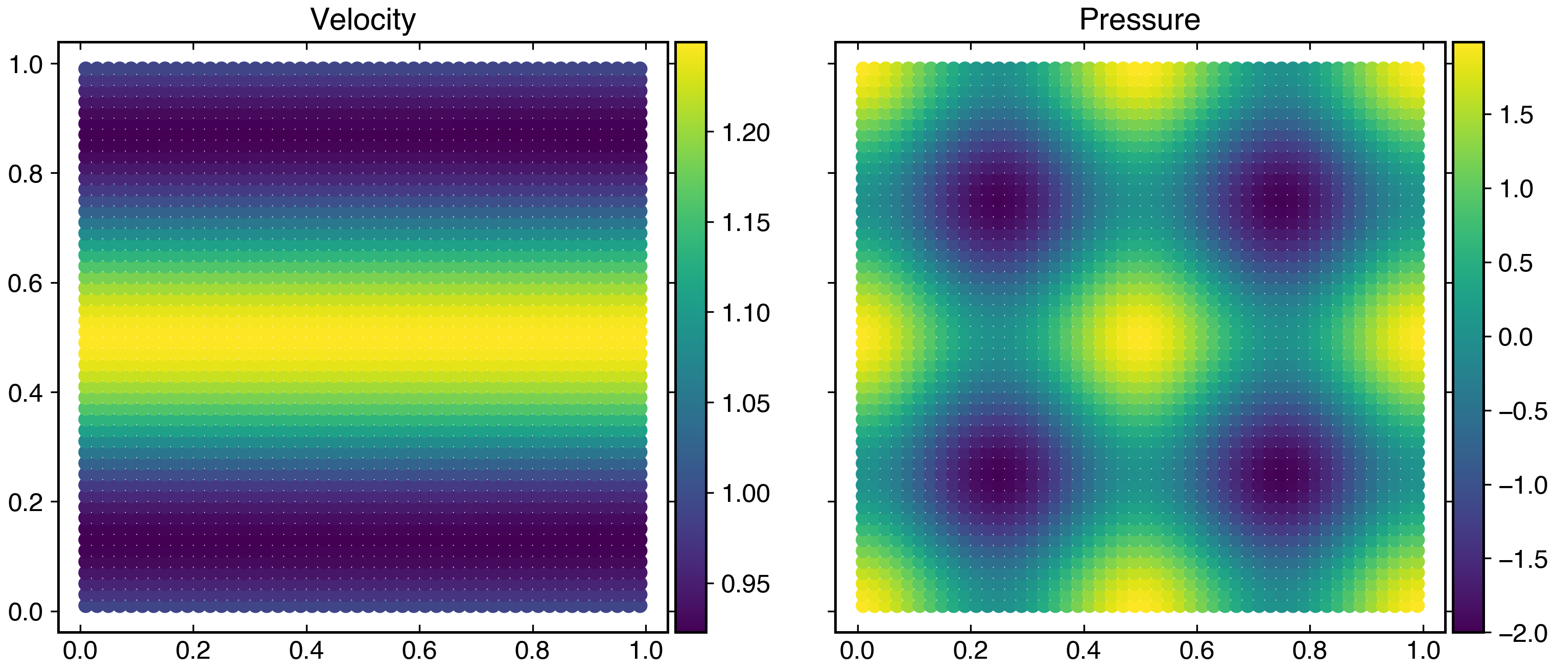
Figure 47: Velocity and pressure contours on the domain in fig. 7 of the MS in eq. 29.

Additionally, we also simulate the wave passing through the inlet and outlet. We also must satisfy the boundary condition. For the inlet, we construct the MS given by

$$\begin{split}u(x,y,t)&=x^{2}y\left(y-1\right)e^{-200\left(x-0.1-40t\right)^{2}}\cos{\left(2\pi y\right)}+1\\ v(x,y,t)&=0.0\\ p(x,y,t)&=\cos{\left(4\pi x\right)}+\cos{\left(4\pi y\right)}\end{split}$$ (30)

In fig. 48, we plot the velocity and pressure contour for the MS in eq. 30.

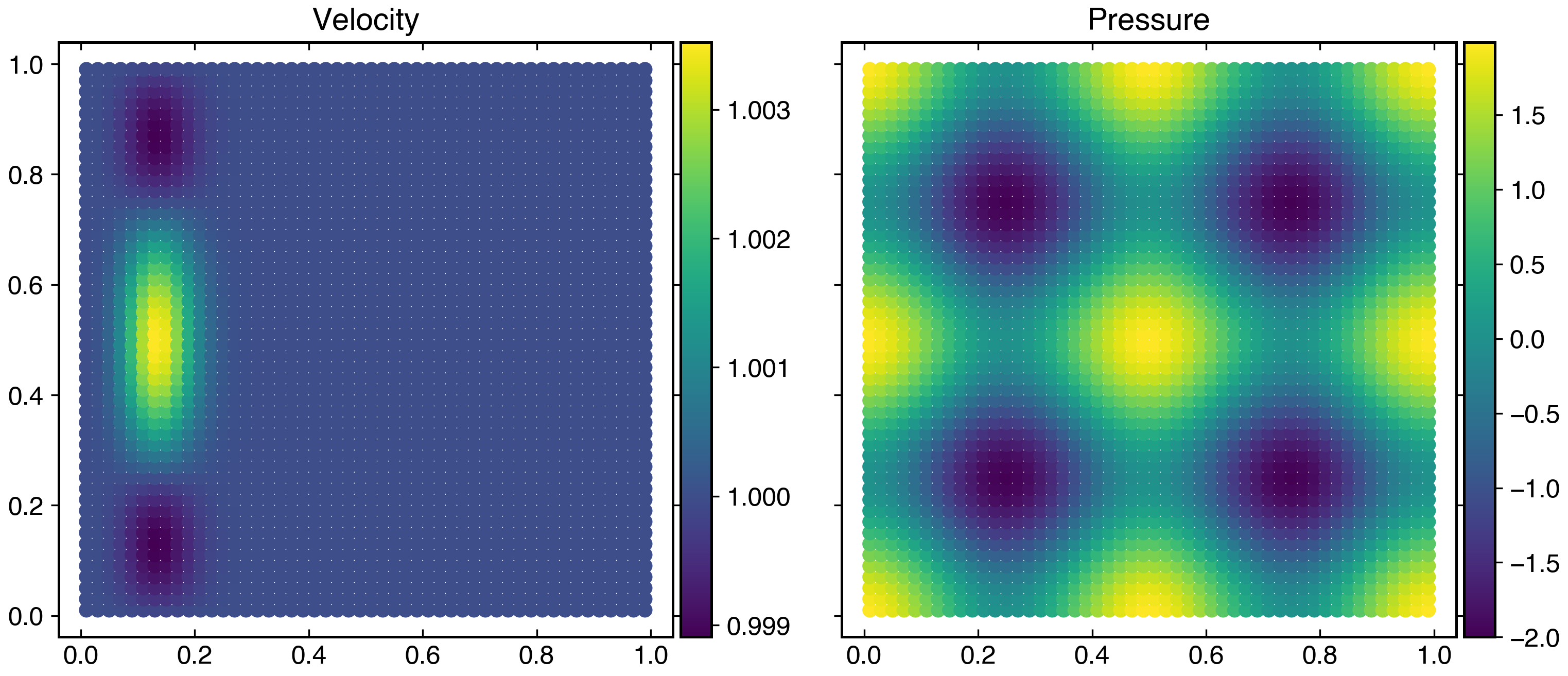
Figure 48: Velocity and pressure contours on the domain in fig. 7 of the MS in eq. 29.

We construct the wave of velocity passing through the outlet given by

$$\begin{split}u(x,y,t)&=(x-1)^{2}y\left(y-1\right)e^{-200\left(x-0.9+40t\right)^{2}}\cos{\left(2\pi y\right)}+1\\ v(x,y,t)&=0.0\\ p(x,y,t)&=\cos{\left(4\pi x\right)}+\cos{\left(4\pi y\right)}\end{split}$$ (31)

In fig. 49, we plot the velocity and pressure generated by the MS in eq. 31.

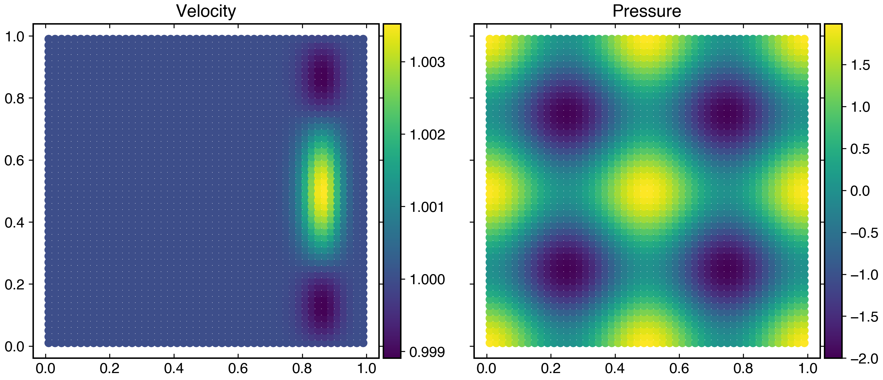
Figure 49: Velocity and pressure contours on the domain in fig. 7 of the MS in eq. 29.

A.5 Inlet and outlet pressure boundary

At the inlet, for pressure ,we make sure that $\nabla p\cdot\mathbf{n}=0$. For inlet as well as the outlet, we use the MS given by

$$\begin{split}u(x,y,t)&=y\left(y-1\right)e^{-10t}\cos{\left(2\pi y\right)}+1\\ v(x,y,t)&=-x\left(x-1\right)e^{-10t}\sin{\left(2\pi y\right)}\\ p(x,y,t)&=y\left(y-1\right)e^{-10t}\cos{\left(2\pi y\right)}\end{split}$$ (32)

In fig. 50, we plot the velocity and pressure contour generated from the MS in eq. 32.

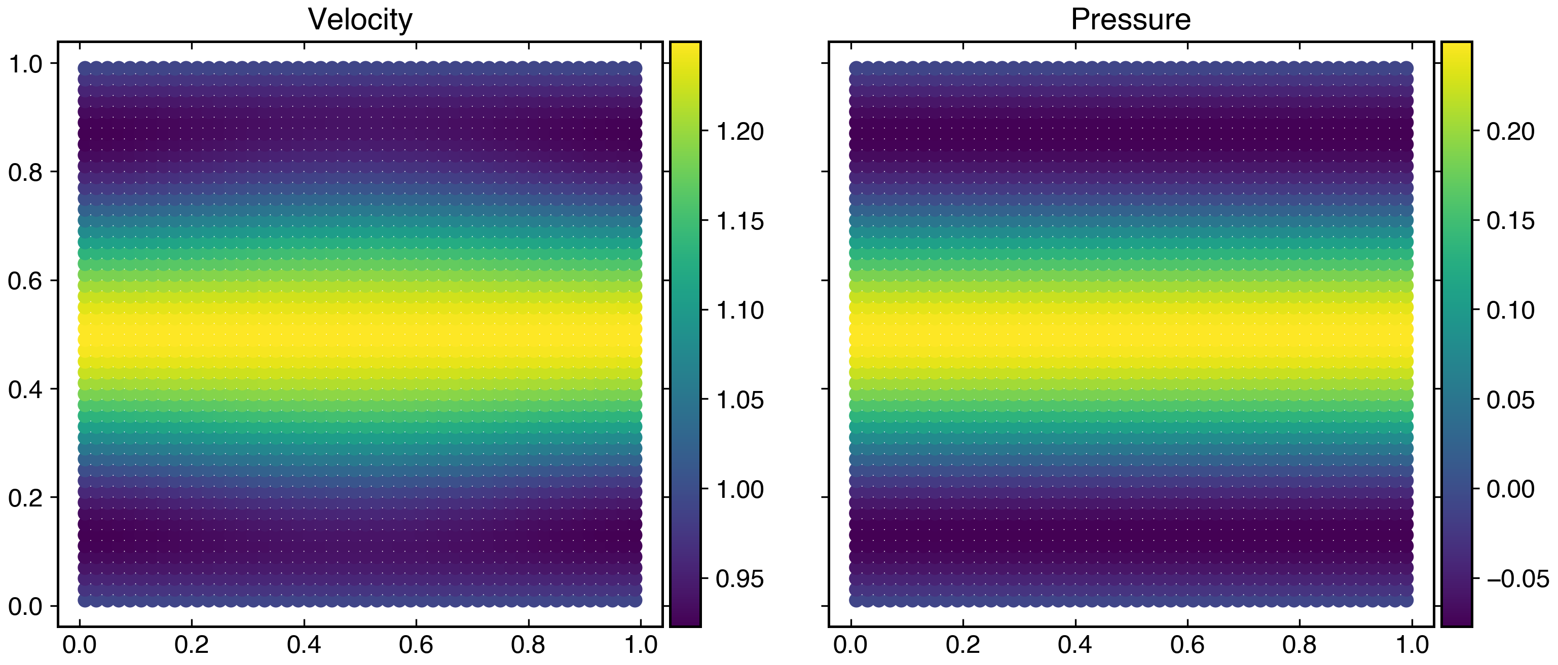
Figure 50: Velocity and pressure contours on the domain in fig. 7 of the MS in eq. 32.

In order to simulate a pressure wave passing through both inlet and outlet, we construct MSs with pressure moving with the artificial speed of sound. For the inlet, we construct the MS given by

$$\begin{split}u(x,y,t)&=y\left(y-1\right)\cos{\left(2\pi y\right)}+1\\ v(x,y,t)&=0.0\\ p(x,y,t)&=x^{2}e^{-200\left(x-0.1-40t\right)^{2}}\cos{\left(2\pi y\right)}\end{split}$$ (33)

In fig. 51, we plot the velocity and pressure generated from the MS in eq. 33.

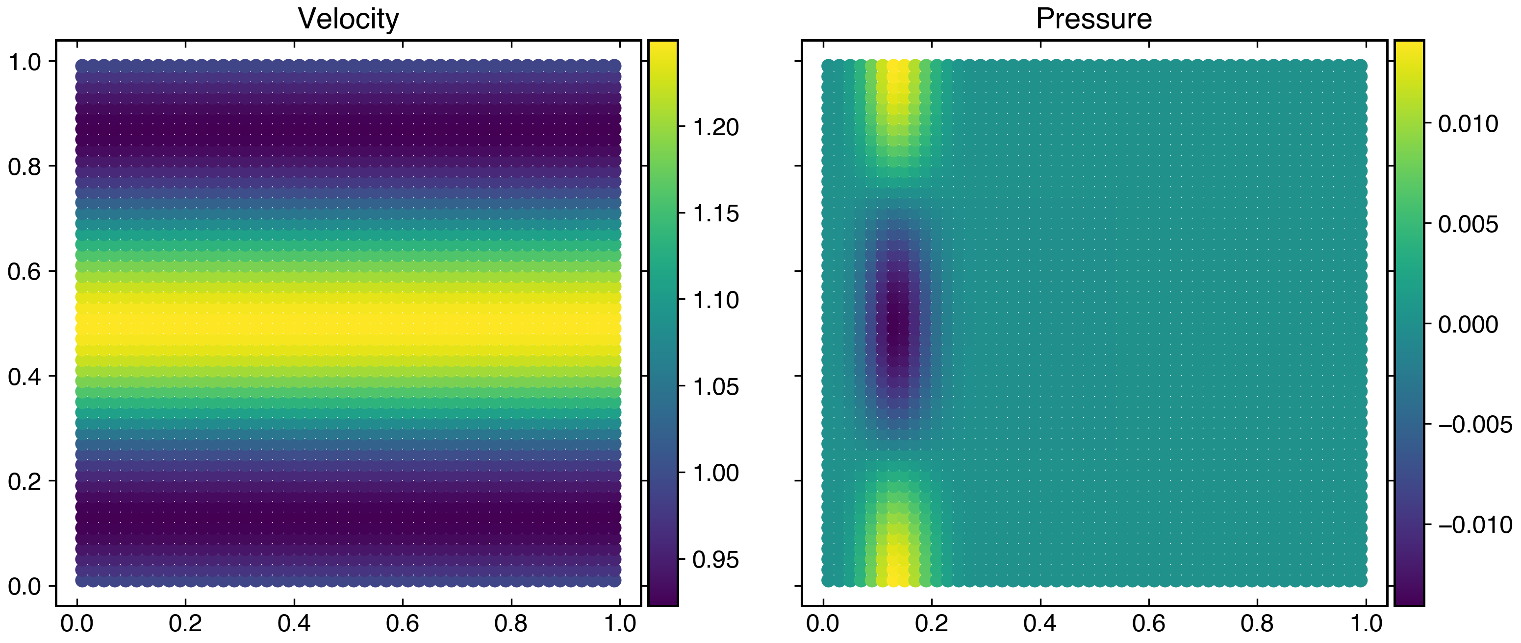
Figure 51: Velocity and pressure contours on the domain in fig. 7 of the MS in eq. 32.

In the case of the outlet, we construct the MS given by

$$\begin{split}u(x,y,t)&=y\left(y-1\right)\cos{\left(2\pi y\right)}+1\\ v(x,y,t)&=0.0\\ p(x,y,t)&=(x-1)^{2}e^{-200\left(x-0.9+40t\right)^{2}}\cos{\left(2\pi y\right)}\end{split}$$ (34)

In fig. 52, we plot the velocity and pressure due to MS in eq. 34.

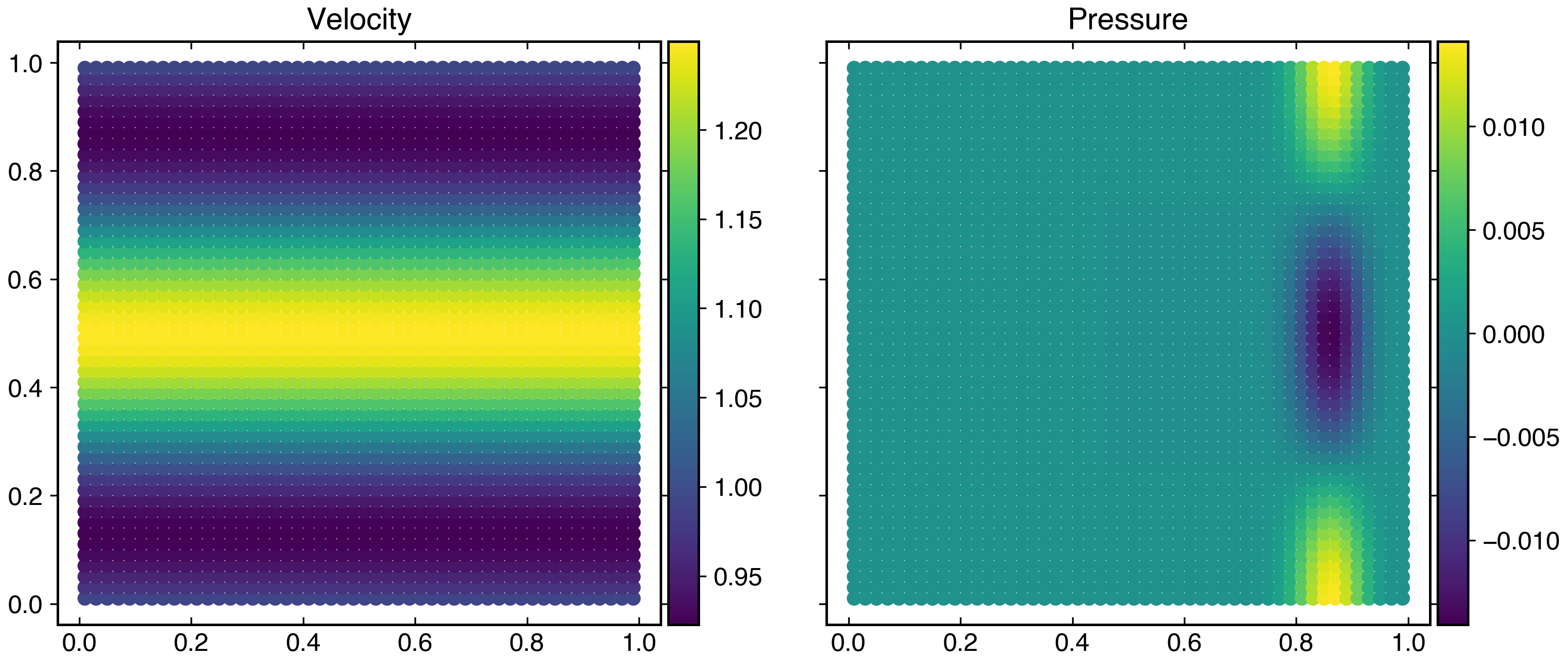
Figure 52: Velocity and pressure contours on the domain in fig. 7 of the MS in eq. 32.

References

- Violeau [2012] Violeau, D.. Fluid mechanics and the SPH method: theory and applications. Oxford University Press; 2012. doi:10.1093/acprof:oso/9780199655526.001.0001.
- Gomez-Gesteria et al. [2010] Gomez-Gesteria, M., Rogers, B.D., Dalrymple, R.A., Crespo, A.J.. State-of-the-art classical SPH for free-surface flows. Journal of Hydraulic Research 2010;84:6–27. doi:10.1080/00221686.2010.9641242.
- Adami et al. [2013] Adami, S., Hu, X., Adams, N.. A transport-velocity formulation for smoothed particle hydrodynamics. Journal of Computational Physics 2013;241:292–307. doi:10.1016/j.jcp.2013.01.043.
- Ramachandran and Puri [2019] Ramachandran, P., Puri, K.. Entropically damped artificial compressibility for SPH. Computers and Fluids 2019;179(30):579–594. doi:10.1016/j.compfluid.2018.11.023.
- Sun et al. [2019] Sun, P., Colagrossi, A., Marrone, S., Antuono, M., Zhang, A.M.. A consistent approach to particle shifting in the -plus-sph model. Computer Methods in Applied Mechanics and Engineering 2019;348:912–934. doi:10.1016/j.cma.2019.01.045.
- Ramachandran et al. [2021] Ramachandran, P., Muta, A., Ramakrishna, M.. Dual-time smoothed particle hydrodynamics for incompressible fluid simulation. Computers & Fluids 2021;227:105031. doi:10.1016/j.compfluid.2021.105031.
- Negi and Ramachandran [2022] Negi, P., Ramachandran, P.. Techniques for second order convergent weakly-compressible smoothed particle hydrodynamics schemes without boundaries. 2022. doi:10.1063/5.0098352.
- Vacondio et al. [2020] Vacondio, R., Altomare, C., De Leffe, M., Hu, X., Le Touzé, D., Lind, S., Marongiu, J.C., Marrone, S., Rogers, B.D., Souto-Iglesias, A.. Grand challenges for Smoothed Particle Hydrodynamics numerical schemes. Computational Particle Mechanics 2020;doi:10.1007/s40571-020-00354-1.
- Violeau and Rogers [2016] Violeau, D., Rogers, B.D.. Smoothed particle hydrodynamics (SPH) for free-surface flows: past, present and future. Journal of Hydraulic Research 2016;54:1–26.
- Takeda et al. [1994] Takeda, H., Miyama, S.M., Sekiya, M.. Numerical Simulation of Viscous Flow by Smoothed Particle Hydrodynamics. Progress of Theoretical Physics 1994;92(5):939–960. doi:10.1143/ptp/92.5.939.
- Maciá et al. [2011] Maciá, F., Antuono, M., González, L.M., Colagrossi, A.. Theoretical Analysis of the No-Slip Boundary Condition Enforcement in SPH Methods. Progress of Theoretical Physics 2011;125(6):1091–1121. doi:10.1143/PTP.125.1091.
- Randles and Libersky [1996] Randles, P., Libersky, L.D.. Smoothed particle hydrodynamics: some recent improvements and applications. Computer methods in applied mechanics and engineering 1996;139(1-4):375–408. doi:10.1016/S0045-7825(96)01090-0.