Lottery Pools: Winning More by Interpolating Tickets without Increasing Training or Inference Cost

Abstract

Lottery tickets (LTs) is able to discover accurate and sparse subnetworks that could be trained in isolation to match the performance of dense networks. Ensemble, in parallel, is one of the oldest time-proven tricks in machine learning to improve performance by combining the output of multiple independent models. However, the benefits of ensemble in the context of LTs will be diluted since ensemble does not directly lead to stronger sparse subnetworks, but leverages their predictions for a better decision. In this work, we first observe that directly averaging the weights of the adjacent learned subnetworks significantly boosts the performance of LTs. Encouraged by this observation, we further propose an alternative way to perform an “ensemble” over the subnetworks identified by iterative magnitude pruning via a simple interpolating strategy. We call our method Lottery Pools. In contrast to the naive ensemble which brings no performance gains to each single subnetwork, Lottery Pools yields much stronger sparse subnetworks than the original LTs without requiring any extra training or inference cost. Across various modern architectures on CIFAR-10/100 and ImageNet, we show that our method achieves significant performance gains in both, in-distribution and out-of-distribution scenarios. Impressively, evaluated with VGG-16 and ResNet-18, the produced sparse subnetworks outperform the original LTs by up to 1.88% on CIFAR-100 and 2.36% on CIFAR-100-C; the resulting dense network surpasses the pre-trained dense-model up to 2.22% on CIFAR-100 and 2.38% on CIFAR-100-C. Our source code can be found at https://github.com/luuyin/Lottery-pools.

Introduction

Deep neural networks (DNNs) have revolutionized various machine learning fields with expressive performance (LeCun et al. 1989; Krizhevsky, Sutskever, and Hinton 2012; Simonyan and Zisserman 2014; He et al. 2016; Silver et al. 2016; Dosovitskiy et al. 2020; Brown et al. 2020; Radford et al. 2021; Fedus, Zoph, and Shazeer 2021; Jumper et al. 2021). While achieving increasingly compelling results, a large concern is the massive parameter count that in billions, even trillions resulting heavy burden on environmental and financial systems (García-Martín et al. 2019; Schwartz et al. 2020; Patterson et al. 2021; Zhang et al. 2022). That motivates many techniques toward the efficiency of DNNs. Among them, sparsity is a leading approach that largely preserves the model performance while achieving appealing compression rates (Mozer and Smolensky 1989; Han, Mao, and Dally 2015; Molchanov et al. 2016; Liu et al. 2022; Chen et al. 2022; Sun et al. 2021; Yuan et al. 2021). A recent work on the Lottery Tickets (LTs) (Frankle and Carbin 2018) discovers the existence of sparse subnetworks within a standard network which can be trained in isolation to match the accuracy of the dense counterpart. These lottery tickets are empirically obtained by iterative magnitude pruning (IMP) at the random dense initialization or early training points called “rewinding” (Frankle et al. 2020). Since being proposed, LTs has become the leading approach to reducing model size while preserving accuracy.

However, LTs is a rather costly process involving multiple iterations of pruning-and-retraining, and once the subnetworks at the target sparsity are reached, the previous subnetworks with lower sparsity are commonly discarded, leading to a big waste of computation. One of the traditional ways that can directly benefit from multiple models in machine learning is ensemble. Ensemble (Hansen and Salamon 1990; Levin, Tishby, and Solla 1990; Fort, Hu, and Lakshminarayanan 2019) is well-known for its compelling performance improvements over independently trained, single networks by combining the predictions of the latter. Yet, ensemble does not directly lead to stronger sparse subnetworks but leverages their predictions to make a better decision. Hence, the benefits of ensemble in the context of LTs will be diluted.

In this paper, we build an efficient and accurate alternative to the naive LTs ensemble that yields subnetworks outperforming the original LTs by a large margin in both, in-distribution and out-of-distribution scenarios. We first observe that directly interpolating weights of the adjacent LTs subnetworks improves the performance of LTs. Inspired by this observation, we sequentially interpolate the weights of the natural “byproducts” of LTs (i.e., the previous subnetworks identified by IMP) with the target subnetwork if they improve accuracy on held-out data, following the recent emerging weight averaging techniques (Izmailov et al. 2018; Wortsman et al. 2022; Rame et al. 2022). This simple interpolating step is able to produce much stronger sparse and dense networks, without incurring any additional training and inference costs. We call our approach “Lottery Pools”. Unlike the original LTs, Lottery Pools harnesses the advantage of all the LTs subnetworks, in turn, to further boost the performance of each of them. This property significantly increases the utility of the identified subnetworks compared with the original LTs, where the previous well-learned subnetworks are usually discarded. Overall, our contributions are summarised as follows:

• Simple weight interpolation between two adjacent subnetworks boosts the performance of LTs. We surprisingly find that adjacent subnetworks of LTs can be linearly interpolated or even averaged into a single subnetwork with higher accuracy while maintaining the same sparsity (shown in Figure 1).

• Towards stronger LTs subnetworks. Encouraged by the above observation, we propose Lottery Pools that selectively interpolate multiple subnetworks into a single subnetwork. Lottery Pools is able to construct stronger subnetworks with much higher accuracy, while maintaining the original sparsity level. Simple as it is, we show that Lottery Pools (Interpolation) surpasses the original LTs by 1.88% and 1.72% on CIFAR-100 with VGG-16 and ResNet-18 respectively.

• Towards stronger dense networks. Besides the improved sparse subnetworks, we can also construct a stronger dense network by averaging the LTs tickets back to the pre-trained dense networks. Our reinforced dense network outperforms the original dense ResNet-18 by 2.22% and the original dense VGG-16 by 1.69% on CIFAR-100.

• Towards Stronger in-distribution and out-of-distribution performance. Thanks to the “ensemble” property of Lottery Pools, the enhanced (sub)networks enjoy a remarkable performance gain over the original LTs/dense model in both in-distribution (ID) predictive accuracy and out-of-distribution (OoD) robustness.

Related Work

Lottery ticket hypothesis. Lottery ticket (LTs) (Frankle and Carbin 2018) conjectures that there exist sparse subnetworks called winning tickets within a dense network, whose performance can match with the dense network when training from the same initialization. Later, weight/learning rate rewinding techniques (Frankle et al. 2020; Renda, Frankle, and Carbin 2020) was proposed to scale up LTs to larger networks and datasets. Evci et al. (2022) demonstrates that training LTs solutions with the same initialization converge to the same basin as the original pruning method that they are derived from. LTs has inspired many follow-up works to understand and extend LTs. Zhou et al. (2019); Ramanujan et al. (2020) successfully found winning tickets at the initialization even without training. Morcos et al. (2019) unveiled that the winning tickets discovered using larger datasets consistently transferred better than those generated using smaller datasets. Besides the original ImageNet classification (Frankle and Carbin 2018), the existence of winning tickets has been broadly verified under diverse fields, such as natural language processing (Gale, Elsen, and Hooker 2019; Chen et al. 2020), generative adversarial networks (Chen et al. 2021), and reinforcement learning (Yu et al. 2019). Unlike LTs, Lottery Pools takes advantage of all the sparse subnetworks to construct stronger subnetworks without increasing any extra training or inference time.

Weight averaging. Model weight averaging has been widely studied in convex optimization and neural networks (Ruppert 1988; Polyak and Juditsky 1992; Zhang et al. 2019). Stochastic Weight Averaging (SWA) (Izmailov et al. 2018) and Exponential Moving Average (EMA) (Polyak and Juditsky 1992) average checkpoints along a single optimization trajectory and can roughly match the prediction ensemble performance. Yin et al. (2022) further generated SWA in the context of sparse training without any pretraining steps. Greedy soup (Wortsman et al. 2022) averages independent dense models across different runs, providing notable improvements.

Weight interpolation, as a more general case of weight averaging, draws explosive interest from the community recently. Nagarajan and Kolter (2019) empirically observed that there exists a linear path between the solutions learned on MNIST dataset with the same initialization. Neyshabur, Sedghi, and Zhang (2020) shown that two models fine-tuned from the same pre-trained model can be linearly connected to match the performance of the single model. Wortsman et al. (2022) proposed learned soup recipe that learns model interpolation by AdamW (Loshchilov and Hutter 2017). Weight interpolation has also been adopted to improve the accuracy of the patching task without compromising accuracy on the supported tasks and transfer learning (Ilharco et al. 2022). Frankle et al. (2020) introduced linear mode connectivity to study the instability of neural networks to the SGD noise introduced during training. They demonstrated that sparse subnetworks discovered by LTs can match the performance of the dense network only when they are stable to SGD noise. Following Frankle et al. (2020), we discover that two linearly connected subnetworks can be interpolated, leading to a more accurate subnetwork without any extra costs.

Ensemble. Ensembles (Hansen and Salamon 1990; Levin, Tishby, and Solla 1990) of neural networks have received large success in terms of the in-distribution accuracy (Perrone and Cooper 1992; Breiman 1996; Dietterich 2000), uncertainty estimation (Lakshminarayanan, Pritzel, and Blundell 2017; Wen, Tran, and Ba 2020), and out-of-distribution robustness (Ovadia et al. 2019; Gustafsson, Danelljan, and Schon 2020). Very recently, Liu et al. (2021) proposed an efficient ensemble framework that combines the predictions of multiple individual subnetworks, surpassing the generalization performance of the naive ensemble. Nevertheless, the ensemble requires performing a forward pass for each model, leading to extra costs.

Table 1: The primary methods contrasted in this work. ${\bm{\mathrm{\tilde{\theta}}}}$ is a subnetwork learned by IMP from different iteration. Cost refers to the memory and computes requirements during inference relative to a single model. All methods require the same training.

Method	Formulation	Cost
Lottery Tickets	$f(\bm{x};{\bm{\mathrm{\tilde{\theta}}}})$	$\mathcal{O}(1)$
Naive Ensemble	$\frac{1}{k}\sum_{i=1}^{k}f(\bm{x};{\bm{\mathrm{\tilde{\theta}}}}_{k})$	$\mathcal{O}(k)$
Lottery Pools	Algorithm 2	$\mathcal{O}(1)$

Methodology

In this section, we introduce “Lottery Pools”, a simple weight interpolation approach that constructs more accurate subnetworks than LTs, without requiring any extra training or inference cost. Different from previous works on interpolation, our goal is to boost the performance of LTs subnetworks (including the pre-trained dense network) while maintaining their desirable sparsity.

We first recap the concept of the lottery ticket hypothesis. Then, we show that directly averaging LTs subnetworks identified at two adjacent IMP iterations leads to stronger subnetworks. Finally, we introduce our Lottery Pools, which is able to improve the accuracy of the original LTs by interpolating subnetworks obtained across different IMP iterations.

Recapping the lottery ticket hypothesis. The lottery ticket hypothesis (Frankle and Carbin 2018) indicates that there exist subnetworks (winning tickets) within dense network initialization such that those lottery tickets could be trained in isolation to the matching performance of their dense counterparts.

To be specific, we denote neural network with parameters $\bm{\mathrm{\theta}}\in\mathbb{R}^{d}$ as $f(\bm{x};\bm{\mathrm{\theta}})$, after $j$ steps of training, there exists a sparse subnetwork characterized by the binary mask $m$ such that $f(\bm{x};m\odot\bm{\mathrm{\theta}}_{j})$ will perform as well as $f(\bm{x};\bm{\mathrm{\theta}})$ after training. The initial results show LTs hold when the subnetwork is trained with the original initialization, i.e. $j=0$. Later results (Frankle et al. 2020) state a rewinding step to a pre-train point ($j>0$) is required on larger datasets. The overall training procedure of LTs is given in Algorithm 1.

Algorithm 1 Pseudocode of LTs

0:  Randomly initialization network $\bm{\mathrm{\theta}}\in\mathbb{R}^{d}$, binary mask $m$, IMP iterations $T$, training steps used for rewinding $j$, pruning rate $p$.

1:  Train $\bm{\mathrm{\theta}}$ to completion; save the weights at $j$ steps $\bm{\mathrm{\theta}}_{j}$.

2:  for pruning iteration $t\in\{1,\ldots,T\}$ do

3:     Prune the lowest magnitude $p$ of weights and update mask $m^{t}$.

4:     Train $m^{t}\odot\bm{\mathrm{\theta}}_{j}$ to completion.

5:  end for

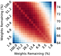
(a) ResNet-18 w/ Rewinding

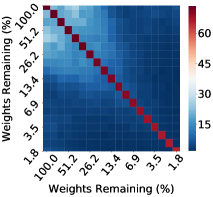
(b) ResNet-18 w/o Rewinding

Figure 1: Accuracy heat map of the averaged LTs on CIFAR-100. Each cell refers to the test accuracy of the averaged subnetworks using the LTs under the sparsity of X-axis and Y-axis. If the averaged subnetwork decreases in sparsity, we prune it to the higher sparsity of its parents.

Algorithm 2 Lottery Pools Interpolation Recipe

Input: The original learned sparse subnetwork ${\bm{\mathrm{\tilde{\theta}}}}_{t}$ from LTs, Candidate Lottery Pools $\mathcal{S}_{t}=\{{\bm{\mathrm{\tilde{\theta}}}_{t\text{-}1}},{\bm{\mathrm{\tilde{\theta}}}_{t\text{+}1}},{\bm{\mathrm{\tilde{\theta}}}_{t\text{+}2}},\cdots\}$, Candidate Coefficient Pools $\mathcal{S}_{c}=\{{\mathrm{\alpha_{1}}},\ldots,{\mathrm{\alpha_{n}}}\}$, The interpolated subnetwork ${\bm{\mathrm{\tilde{\theta}}}_{Inter}}$ during greedy search.

Output: Final interpolated subnetwork ${\bm{\mathrm{\tilde{\theta}}}_{best}}$ has the same sparsity with ${\bm{\mathrm{\tilde{\theta}}}_{t}}$.

1:  $\mathcal{S}_{t}\leftarrow\{{\bm{\mathrm{\tilde{\theta}}}_{t\text{-}1}},{\bm{\mathrm{\tilde{\theta}}}_{t\text{+}1}},{\bm{\mathrm{\tilde{\theta}}}_{t\text{+}2}},\cdots\}$ $\triangleright$ Create Candidate Lottery Pools, and sort all candidates by their adjacence to ${\bm{\mathrm{\tilde{\theta}}}_{t}}$

2:   $\mathcal{S}_{c}\leftarrow\{{\mathrm{\alpha_{1}}},\ldots,{\mathrm{\alpha_{n}}}\}$ $\triangleright$Create Candidate Coefficient Pools

3:  ${\bm{\mathrm{\tilde{\theta}}}_{best}}\leftarrow{\bm{\mathrm{\tilde{\theta}}}}_{t}$

4:  for ${\bm{\mathrm{\tilde{\theta}}}_{i}}\in\mathcal{S}_{t}$ do $\triangleright$ Greedily search the candidate LTs subnetworks for interpolation

5:     ${\alpha}_{best}\leftarrow\operatorname*{arg\,max}_{j}\mathsf{ValAcc}\left(\mathsf{MagnitudePruning}\left(\mathrm{\alpha}_{j}\bm{\mathrm{\tilde{\theta}}}_{best}+(1-{\mathrm{\alpha}_{j}})\bm{\mathrm{\tilde{\theta}}}_{i}\right)\right),{\mathrm{\alpha}_{j}}\in\mathcal{S}_{c}$ $\triangleright$Search for the best coefficient

6:      ${\bm{\mathrm{\tilde{\theta}}}_{Inter}}\leftarrow\mathsf{MagnitudePruning}\left(\mathrm{\alpha}_{best}\bm{\mathrm{\tilde{\theta}}}_{best}+(1-{\mathrm{\alpha}}_{best})\bm{\mathrm{\tilde{\theta}}}_{i}\right)$ $\triangleright$Interpolating using ${\alpha}_{best}$

7:     if $\mathsf{ValAcc}\left({\bm{\mathrm{\tilde{\theta}}}_{Inter}}\right)\geq\mathsf{ValAcc}\left({\bm{\mathrm{\tilde{\theta}}}_{best}}\right)$

8:             then ${\bm{\mathrm{\tilde{\theta}}}_{best}}\leftarrow{\bm{\mathrm{\tilde{\theta}}}_{Inter}}$ $\triangleright$Update the best interpolated subnetwork

9:  end for

Simple weight averaging boosts the performance of LTs. Recently, the work on model soup (Wortsman et al. 2022) shows that averaging models fine-tuned from the same pre-trained model provides substantial performance improvements. Since the LTs subnetworks at different sparsities are also fine-tuned from the same pre-trained dense model, we hypothesize that these subnetworks can also be averaged for better performance.

Let’s simplify the sparse subnetwork parameters under a mask $m^{t}\odot{\bm{\mathrm{\theta}}}$ as $\tilde{\bm{\mathrm{\theta}}}$ for simplicity. To verify our hypothesis, we average two LTs subnetworks with different sparsities (assuming sparsity of $\tilde{\bm{\mathrm{\theta}}}_{1}$ is higher than sparsity of $\tilde{\bm{\mathrm{\theta}}}_{2}$) across all the learned subnetworks, i.e., $\frac{\tilde{\bm{\mathrm{\theta}}}_{1}+\tilde{\bm{\mathrm{\theta}}}_{2}}{2}$. To address the sparsity decrease caused by average, we further use magnitude pruning $\frac{\tilde{\bm{\mathrm{\theta}}}_{1}+\tilde{\bm{\mathrm{\theta}}}_{2}}{2}$ to the same sparsity as $\tilde{\bm{\mathrm{\theta}}}_{1}$ following (Yin et al. 2022). We consider two widely used settings for LTs: with rewinding and without rewinding. We report the results of ResNet-18 on CIFAR-100 within a heat map in Figure 1 and put the results of VGG-16 in the Appendix.

As we can see, rewinding matters for the improved performance of weight averaging. With rewinding, simple averaging subnetworks from nearby IMP iterations could achieve better performance than the original LTs subnetworks (the diagonal cells), and the closer two subnetworks are located, the larger performance gains the averaged subnetworks tend to achieve. In stark contrast, we observe a significant accuracy drop without rewinding, across all sparsities. This observation is in line with the findings from Frankle et al. (2020) that large-scale settings are unstable to SGD noise at initialization according to linear interpolation. Thereby, we confirmed that our hypothesis holds in the context of rewinding.

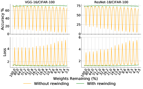
Figure 2: Liner interpolation between learned subnetworks from dense network to extremely low density.

Lottery Pools

Inspired by the above observation, we introduce Lottery Pools, a simple weight interpolation approach on LTs that leverages the subnetworks obtained across different IMP iterations. Lottery Pools has two key ideas: (1) Interpolating weights instead of simply averaging; (2) Sequentially searching over all the candidate LTs subnetworks and coefficients for interpolation.

Firstly, Lottery Pools goes beyond weight averaging and probes a more general variant of weight connection – weight interpolation. Linear weight interpolation has been previously used to study dense networks (Nagarajan and Kolter 2019; Neyshabur, Sedghi, and Zhang 2020). Here, we adopt it to improve the accuracy of sparse LTs subnetworks. We follow (Frankle et al. 2020) and determine that two LTs subnetworks are linear mode connected if there exists a linear path between them. The two subnetworks thus could be interpolated for accuracy improvement. The subnetwork created by interpolating is given by:

$$\bm{\mathrm{\tilde{\theta}}}_{inter}=\mathrm{\alpha}\bm{\mathrm{\tilde{\theta}}}_{1}+(1-{\mathrm{\alpha}})\bm{\mathrm{\tilde{\theta}}}_{2}$$ (1)

We argue that directly averaging two subnetworks ($\alpha=0.5$) might not be the optimal option, since the local linearly-connected minimum may lie in the sides of the linear path rather than in the right middle. To prove this, we linearly interpolate two adjacent LTs subnetworks, with various coefficients $\alpha\in[0,1]$. We set the increments of $\alpha$ as $0.1$ to create 9 interpolated subnetworks between two LTs subnetworks. The test loss/error are reported in Figure 2. The best accuracy is achieved at the middle points of the linear path in most cases (the middle part of the green lines) with exceptions at the highest and lowest sparsities (the endpoints of the green lines) where weight average achieves no better accuracy than interpolation. Again, interpolation without weight rewinding (yellow lines) fails to find such linear paths between two subnetworks.

Moreover, Figure 1 and 2 present that the accuracy of the interpolated subnetworks varies across different subnetworks pairs and different interpolation coefficients. While it is possible to adopt gradient-based optimization to learn the optimal subnetworks and coefficients, the cost is rather expensive. We instead choose a more practical way: greedily searching for interpolated subnetworks and the corresponding coefficients. Given a target LTs subnetwork ${\bm{\mathrm{\tilde{\theta}}}_{t}}$ learned at the $t$ iteration of IMP, we sequentially interpolate it with the rest of the subnetworks (Candidate Lottery Pools). For each candidate subnetwork, we search the best coefficients $\alpha$ over 11 candidates from 0.05 to 0.95 (Candidate Coefficient Pools). Please refer to the Appendix for more details. We only keep the incoming subnetwork for interpolation if its accuracy on the held-out set does not decrease.

Instead of loading all the candidate subnetworks in the memory (Wortsman et al. 2022), we apply a more memory-friendly search approach. Specifically, we iteratively interpolate one of the subnetworks in the Candidate Lottery Pools with our target subnetwork ${\bm{\mathrm{\tilde{\theta}}}_{t}}$ and let the resulting subnetwork being our new target subnetwork, i.e. ${\bm{\mathrm{\tilde{\theta}}}}_{t}\leftarrow{\bm{\mathrm{\tilde{\theta}}}_{inter}}$, until we have searched all the subnetworks. This operation allows us to accomplish the interpolation operation across all the candidate subnetworks by maintaining only one extra copy of the interpolated weights.

In summary, Lottery Pools is a two-step procedure for constructing stronger LTs subnetworks. Step 1: Perform the standard Lottery Tickets method; Step 2: Linearly interpolate the original LTs subnetworks to produce stronger sparse subnetworks. Please note that we adopt magnitude weight pruning to remove the weights with the smallest magnitude after each interpolation to maintain the same sparsity level as the original LTs.

Experiments

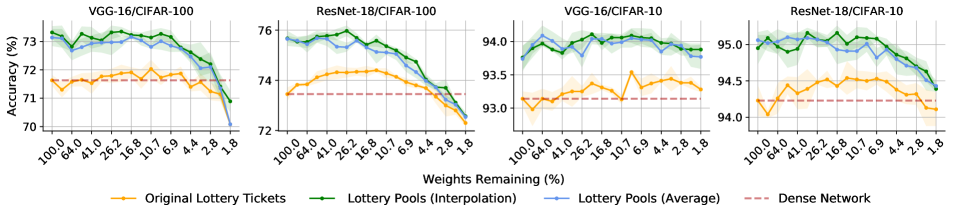
(a) Test accuracy % of the original LTs and Lottery Pools on CIFAR-10/100.

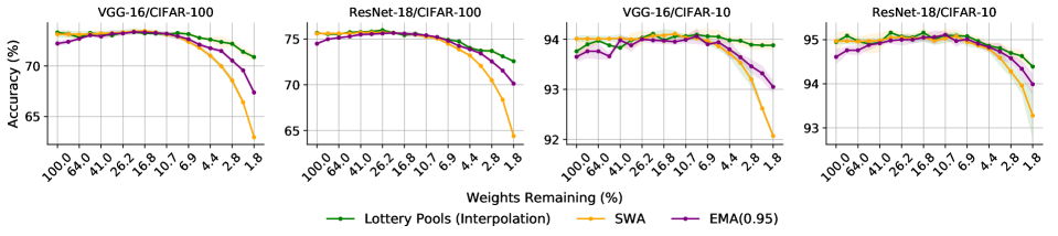
(b) Comparison with the strong weight averaging baselines: SWA and EMA.

(c) Test accuracy % of the original LTs and Lottery Pools on CIFAR-10-C and CIFAR-100-C.

Figure 3: Evaluation of Lottery Pools.

To verify the effectiveness of Lottery Pools, we evaluate it with three popular model structures VGG-16, ResNet-18 and ResNet-34 on various datasets, including CIFAR-10 and CIFAR-100 and ImageNet.

Table 2: Implementation details, including: IMP iteration count, rewinding epochs, learning rate (LR), batch size (BS), learning rate drop (LR Drop), training epochs (Epoch), etc.

Network	Dataset	Epoch	BS	LR	LR Drop, Epochs	Warmup	Rewinding	IMP iterations
ResNet-18	CIFAR-10/100	182	128	0.1	10x, [91, 136]	-	9 Epochs	19
VGG-16	CIFAR-10/100	182	128	0.1	10x, [91, 136]	-	9 Epochs	19
ResNet-18/34	ImageNet	90	1024	$0.4$	10x, [30,60,80]	5 Epochs	5 Epochs	9

Experiments setup. Since our method directly performs weight interpolation over the subnetworks produced by LTs rewinding, our most direct baseline is the standard LTs rewinding. Following the common rewinding setting used in Frankle et al. (2020); Chen et al. (2020), we rewind the LTs roughly to the 5% training time. We summarize the implementation details for LTs in table 2. To highlight the performance difference between weight interpolation and weight averaging, we implement two variants of Lottery Pools: Lottery Pools (Interpolation) and Lottery Pools (Average), the latter applies direct averaging instead of interpolation in the second step of Lottery Pools. The results are illustrated in Figure 3(a). All the reported results are averaged over 3 independent runs.

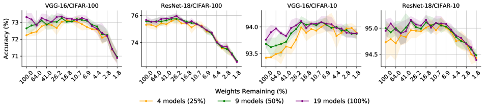
Figure 4: Test accuracy % of different candidate model count.

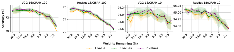
Figure 5: Test accuracy % of different candidate interpolation coefficient count.

Comparison with the original LTs. Overall, we see a clear performance gain from Lottery Pools over the original LTs under different sparsity levels (including the dense network), and Lottery Pools (Interpolation) achieves better performance than Lottery Pools (Average) due to the searched optimal interpolation value. Impressively, Lottery Pools (Interpolation) achieves up to 1.88% and 1.72% accuracy increase over the original LTs with VGG-16 and ResNet-18 on CIFAR-100, respectively. Even on the relatively more saturated CIFAR-10, we still observe up to 0.93% and 1.05% performance gains with VGG-16 and ResNet-18. We highlight that Lottery Pools also outperforms LTs in even extremely sparse situations. For instance, Lottery Pools brings 0.81% higher accuracy over the LTs with VGG-16 on CIFAR-100 and 0.6% higher accuracy on CIFAR-10, with only 1.8% weights. It is quite encouraging to see that Lottery Pools can still improve performance when the interpolating space is extremely small. Besides, by averaging the learned LTs subnetworks back to the pre-trained dense model, Lottery Pools (interpolation) could also construct stronger dense networks, which outperform the original dense ResNet-18 by 2.22% and the original dense VGG-16 by 1.69% on CIFAR-100. We report the results with ResNet-18/34 on ImageNet in the Appendix due to the limited space, where Lottery Pools also consistently outperforms LTs.

Comparison with weight averaging baselines. We further compare our method with two strong weight averaging baselines: SWA and EMA. SWA (Izmailov et al. 2018) averages the weights of multiple networks along a single optimization trajectory. By setting the averaging coefficient to $\frac{1}{n+1}$ where $n$ is the current model number, it achieves the same results of averaging across all the models while maintaining the memory consumption as just two DNNs. The exponential moving average (EMA) (Polyak and Juditsky 1992; Kingma and Ba 2014; Karras et al. 2017) average the weights of a series of models exponentially using a fixed decay factor, which was set to 0.95 in this experiment. As these baselines are all designed for dense model averaging, the same as Lottery Pools, we alter EMA and SWA by pruning the interpolated model to the sparsity of the original LHs during interpolating. In fact, both SWA and EMA could be regarded as special cases of linear interpolation that use specific averaging coefficients and decay factors for weight interpolating.

As shown in Figure 3(b), our method clearly outperforms the other baselines by a large margin, especially in highly sparse situations. That apparently comes from two possible reasons. Firstly, EMA and SWA use pre-chosen coefficient values, which might not generate all the subnetworks, whereas Lottery Pools searches for the optimal values for each subnetwork. Secondly, Lottery Pools greedily searches for potential subnetworks to interpolate, which can eliminate the negative effects of subnetworks that are adding networks within the different loss basins for interpolation.

Out-of-distribution robustness. Beyond the in-distribution accuracy, we highlight that Lottery Pools also improves the performance of LTs in the OoD scenario. We train Lottery Pools with standard CIFAR-10 and CIFAR-100 and test it on CIFAR-10-C and CIFAR-100-C, respectively. As shown in Figure 3(c), Lottery Pools improves the OoD robustness than the original LTs by a large margin with both dense and sparse subnetworks. Remarkably, it improves the dense ResNet-18 by 2.38% on CIFAR-100, and by 2.12% with VGG-16 on CIFRA-10. For sparse subnetworks, Lottery Pools achieves up to 2.27% performance gain with VGG-16, and 2.36% with ResNet-18 on CIFAR-100. This result indicates that our interpolated subnetworks are able to inherit the appealing properties of model ensemble, e.g., good OoD robustness.

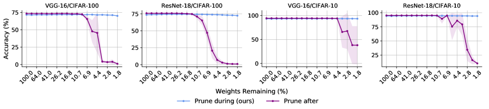
Figure 6: Comparison between prune after interpolating and prune during interpolating.

Figure 7: Comparison between Lottery Pools and the output ensemble.

Extensive Analysis

Candidate lottery pools count. In this section, we study how the number of candidate tickets count, i.e., $\|{S}_{t}\|_{0}$ affects the achieved model’s performance. In the main experiment section, we take advantage of all the learned networks across different IMP iterations for interpolation. Here, we alter the count of networks in ${S}_{t}$ as 4, 9, 19, which represents 25%, 50%, 100% total number of possible networks. All the networks are still sorted in the order of the adjacency to the target lottery tickets in ${S}_{t}$. The results are shown in Figure 4. Not surprisingly, more candidate tickets tend to yield better performance in general. Besides, the performance gap between different Candidate Lottery Pools counts in the dense model is more significant than in the sparse situations.

Candidate interpolation coefficient count. Here, we study how the interpolation coefficient count affects the Lottery Pool’s performance. Intentionally, more candidates would be more likely to provide a proper coefficient by searching and thereby gain larger performance improvements. To confirm this hypothesis, we compare Lottery Pools using different candidate coefficient counts, including 1 ($\alpha$ =[0.5]), 3 ($\alpha$=[0.05, 0.5, 0.95]), 7 ($\alpha$=[0.05,0.1,0.3,0.5,0.7,0.9,0.95]). Therefore, when using coefficient count as 1, Lottery Pools scales to Lottery Pools (Average). The results are illustrated in Figure 4. Lottery Pools (Average) with 1 candidate (yellow lines) achieves the lowest accuracy in general, compared to the settings with more candidates, due to its limited search space. Lottery Pools with 7 candidates outperforms the one with 3 candidates, but only with marginal gains.

When to Prune. We study when to prune the interpolated subnetwork to target sparsity. In the default setting of Lottery Pools, we perform the pruning operation every once when we interpolate a subnetwork during the greedy search (line 5, 6 in Algorithm 2), which we called prune during. Another option would be first greedy interpolating all the searched subnetworks and then pruning the achieved subnetwork to the target sparsity, namely prune after. We compare these two methods in Figure 6. As we can see, the performance of prune after drops dramatically at the high sparsity while prune during keeps a steady high accuracy across all the sparsities. The reason might be in prune after, we greedy search for the best un-pruned interpolated networks regardless of their performance at the target sparsity. Whereas the prune during operation in greedy search keeps the interpolated networks always having good performances at desirable sparsity level.

Comparison with output ensemble. This section compares the performance of Lottery Pools with the output ensemble, i.e. averaging the digit of various subnetworks for inference (Huang et al. 2017; Garipov et al. 2018). For every learned subnetwork from IMP, we collect the other two identified subnetworks from most adjacent iterations to perform the Lottery Pools and output ensemble. The results are reported in Figure 7. As we can see, our Lottery Pools could match the performance of the output ensemble, with no additional computational cost or memory relative to a single subnetwork during inference.

Conclusion

In this paper, we explore a new perspective to leverage the existing learned LTs subnetworks by interpolation. We call this approach Lottery Pools. Without increasing training or inference costs, a network can be identified with significant performance improvements for in- and out-distribution scenarios. Impressively, Lottery Pools is capable of creating not only stronger subnetworks that maintain the original LTs sparsity level but also stronger dense networks. Extensive experiments verify the effectiveness of Lottery Pools across various network architectures with VGG-16 and ResNet-18/34 on CIFAR-10/100 and ImageNet.

Appendix A Results of ImageNet

In this appendix, we compare the performance of Lottery Pools against the original Lottery Tickets on ImageNet and report the results in FigureA8. Overall, we notice a clear performance gain from Lottery Pools over the original LTs at a set of sparsities.

To be specific, by adopting Lottery Pools (Interpolation), we observe up to 0.55% and 0.63% improvements to the original sparse LTs on ResNet-18 and ResNet-34, respectively. Besides, the constructed stronger dense networks outperform the original dense ResNet-18 and ResNet-34 by 0.71% and 0.76%, respectively. All these results demonstrated Lottery Pools’ effectiveness on the large-scale dataset.

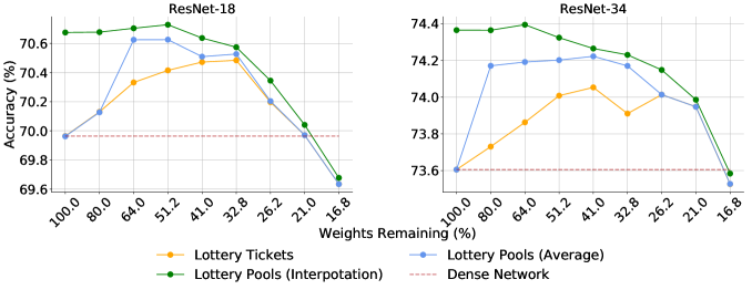
Figure A8: Test accuracy % of original Lottery Tickets and Lottery Pools on ImageNet.

.

Appendix B Accuracy Heat Map of VGG-16

The accuracy heat map of VGG-16 is reported in Figure B9. Here, we observe a similar pattern to the results of Resnet-18 (Figure 1 in the main paper). First, we notice that rewinding is necessary for performance gain using weight averaging. Secondly, the averaged subnetwork’s performance highly depends on its parents’ IMP iteration adjacency. The closer IMP iterations two LTs are from, the better their averaged subnetwork performs. Under rewinding, weight averaging could achieve higher accuracy than the original LTs subnetwork at the same sparsity level if the parent subnetworks are close enough in IMP iteration.

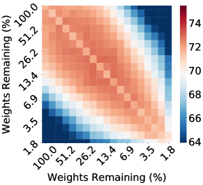
(a) VGG-16 w/ Rewinding

(b) VGG-16 w/o Rewinding

Figure B9: Accuracy heat map of the averaged LTs on CIFAR-100. Each cell refers to the test accuracy of the averaged subnetworks using the LTs under the sparsity of X-axis and Y-axis. If the averaged subnetwork decreases in sparsity, we prune it to the higher sparsity of its parents.

Appendix C Candidate Interpolation Coefficients

In Table 3, we report the Candidate Interpolation Coefficients used in the main experiments of this work. We apply 12 candidate coefficient values ranging from 0.05 to 0.95 to enlarge the optimal value searching space. In Table 4, we show the values adopted in the chapter “Extensive Analysis” of the main paper, where the effect of interpolation coefficient count on Lottery Pools’ performance is studied.

Table 3: Candidate interpolation coefficient in main experiments.

Network	Dataset	Coefficient Count	Coefficient Values
ResNet-18/VGG-16	CIFAR-10/100	11	0.05, 0.1, 0.2, 0.3, 0.4, 0.5
ResNet-18/34	ImageNet		0.6, 0.7, 0.8, 0.9, 0.95

Table 4: Candidate interpolation coefficient in extensive analysis.

Network	Dataset	Coefficient Count	Coefficient Values
ResNet-18/VGG-16	CIFAR-10/100	1	0.5
ResNet-18/VGG-16	CIFAR-10/100	3	0.05, 0.5, 0.95
ResNet-18/VGG-16	CIFAR-10/100	7	0.05, 0.1, 0.3, 0.5, 0.7, 0.9, 0.95

Appendix D Dataset Details

We reported the datasets details, including the number of classes, the size of training, validation and testing sets on CIFAR-10, CIFAR-100, and ImageNet in Table 5. As there are no publicly available labeled sets for testing in these datasets, we use original validation sets for testing, split 10% of the training sets as hold-out validation sets, and use the rest of the training sets for training.

Table 5: Datasets Details.

	Size of the set used for
Dataset	Training	Validation	Testing	Number of classes
CIFAR-10	45,000	5,000	10,000	10
CIFAR-100	45,000	5,000	10,000	100
ImageNet	1,255,167	26,000	50,000	1,000

Appendix E Lottery Tickets Implementation Details

In Table 6 and Table 7, we report the implementation details of creating Lottery Tickets subnetworks that are used for interpolating in Lottery Pools. The reported hyperparameters include total training epochs (Epoch), learning rate (LR), batch size (BS), learning rate drop (LR Drop), weight decay (WD), SGD momentum (Momentum), IMP iteration count, IMP weight pruning fraction and the rewinding epochs, etc.

Computation resources. The experiments on ImageNet were performed with 4 NVIDIA Tesla A100 GPUs, and the experiments on CIFAR-10/100 were run on a single A100 GPU.

Implementation details on CIFAR-10/100. .

Table 6: Implementation hyperparameters of Lottery Tickets on CIFAR-10/100.

Model	Epoch	BS	LR	LR Drop, Epochs	Optimizer	WD	Momentum	Warmup (epochs)	Rewinding (epochs)	IMP iterations (epochs)	Pruning Fraction (%)
VGG-16	182	128	0.1	10x, [91, 136]	SGD	0.9	1e-4	-	9	19	20
ResNet-18	182	128	0.1	10x, [91, 136]	SGD	0.9	1e-4	-	9	19	20

Implementation details on ImageNet.

Table 7: Implementation hyperparameters of Lottery Tickets on ImageNet.

Model	Epoch	BS	LR	LR Drop, Epochs	Optimizer	WD	Momentum	Warmup (epochs)	Rewinding (epochs)	IMP iterations (epochs)	Pruning Fraction (%)
ResNet-18	90	1024	0.4	10x, [30, 60, 80]	SGD	0.9	1e-4	5	5	9	20
ResNet-34	90	1024	0.4	10x, [30, 60, 80]	SGD	0.9	1e-4	5	5	9	20

Appendix F Algorithm of Lottery Pools (Average)

When applying a fixed interpolation value of 0.5 instead of the searched optimal one within the Candidate Coefficient Pools, the Lottery Pools (Interpolation) turns into its variant, the Lottery Pools (Average) that is described in Algorithm 3.

Lottery Pools (Interpolation) tends to achieve better performance than Lottery Pools (Average) by using the searched optimal value for interpolating, while Lottery Pools (Average) is benefited from efficiency due to simple averaging.

Algorithm 3 Lottery Pools Average Recipe

Input: The original learned sparse subnetwork ${\bm{\mathrm{\tilde{\theta}}}}_{t}$ from LTs, Candidate Lottery Pools $\mathcal{S}_{t}=\{{\bm{\mathrm{\tilde{\theta}}}_{t\text{-}1}},{\bm{\mathrm{\tilde{\theta}}}_{t\text{+}1}},{\bm{\mathrm{\tilde{\theta}}}_{t\text{+}2}},\cdots\}$, The averaged subnetwork ${\bm{\mathrm{\tilde{\theta}}}_{Inter}}$ during greedy search.

Output: Final averaged subnetwork ${\bm{\mathrm{\tilde{\theta}}}_{best}}$ that has the same sparsity with ${\bm{\mathrm{\tilde{\theta}}}_{t}}$.

1:  $\mathcal{S}_{t}\leftarrow\{{\bm{\mathrm{\tilde{\theta}}}_{t\text{-}1}},{\bm{\mathrm{\tilde{\theta}}}_{t\text{+}1}},{\bm{\mathrm{\tilde{\theta}}}_{t\text{+}2}},\cdots\}$ $\triangleright$ Create Candidate Lottery Pools, and sort all candidates by their adjacence to ${\bm{\mathrm{\tilde{\theta}}}_{t}}$

2:  ${\bm{\mathrm{\tilde{\theta}}}_{best}}\leftarrow{\bm{\mathrm{\tilde{\theta}}}}_{t}$

3:  for ${\bm{\mathrm{\tilde{\theta}}}_{i}}\in\mathcal{S}_{t}$ do $\triangleright$ Greedily search the candidate LTs subnetworks for averaging

4:      ${\bm{\mathrm{\tilde{\theta}}}_{Inter}}\leftarrow\mathsf{MagnitudePruning}\left(\frac{\bm{\mathrm{\tilde{\theta}}}_{best}+\bm{\mathrm{\tilde{\theta}}}_{i}}{2}\right)$ $\triangleright$Average

5:     if $\mathsf{ValAcc}\left({\bm{\mathrm{\tilde{\theta}}}_{Inter}}\right)\geq\mathsf{ValAcc}\left({\bm{\mathrm{\tilde{\theta}}}_{best}}\right)$

6:             then ${\bm{\mathrm{\tilde{\theta}}}_{best}}\leftarrow{\bm{\mathrm{\tilde{\theta}}}_{Inter}}$ $\triangleright$Update the best averaged subnetwork

7:  end for

Appendix G Diversity analysis.

We plot the prediction disagreement matrix across the learned subnetwork from IMP across different iterations in Figure G10. We can see that the LTs subnetworks behave similarly to their neighbor subnetworks with small prediction disagreement, and such disagreement gradually increases as their distance becomes larger and larger in the context of IMP. The results could explain the phenomena of Figure 1 as a larger diversity indicates it is more likely that the subnetworks are located in the different basins, where weight interpolation does not provide satisfactory performance (Neyshabur, Sedghi, and Zhang 2020; Yin et al. 2022).

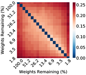
(a) VGG-16/CIFAR-100

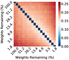
(b) ResNet-18/CIFAR-100

Figure G10: Prediction disagreement between lottery tickets at the different sparsity levels. Each block in the heatmap shows the fraction of labels on which the predictions from different lottery tickets disagree.

Appendix H Results Tables

Here we report the performance details of Lottery Pools, EMA, SWA and original Lottery tickets on CIFAR-10/100 in Table 8 and Table 9. The performance details on ImageNet are reported in Table 10. We apply the decay factor of 0.95 in EMA. For a fair comparison, EMA and SWA are modified by pruning the interpolated models to the sparsity of the original LHs during interpolating. The reported accuracy on CIFAR-10/100 is averaged over 3 independent runs, while we only run the experiments on ImageNet once due to the limited resources.

Compared with the original LTs, Lottery Pools achieves universal performance improvements at all sparsity levels on both ImageNet and CIFAR-10/100 datasets. Compared with the other two baselines (SWA and EMA), our Lottery Pools outperforms these baselines in all cases on ImageNet, and in most cases (60/76) on CIFAR-10/100.

Table 8: Accuracy (%) of Lottery Pools, the original Lottery Tickets, EMA and SWA on CIFAR-10/100 (1).

Dataset	Network	Method	Weights Remaining%
			100	80	64	51.20	40.96	32.77	26.21	20.97	16.78
CIFAR-100	VGG-16	Lottery Pools (interpolation)	73.32$\pm$0.22	73.18$\pm$0.38	72.82$\pm$0.17	73.27$\pm$0.26	73.13$\pm$0.38	73.04$\pm$0.20	73.32$\pm$0.24	73.35$\pm$0.16	73.23$\pm$0.13
		Lottery Pools (Average)	73.14$\pm$0.30	73.11$\pm$0.33	72.68$\pm$0.34	72.80$\pm$0.30	72.93$\pm$0.29	72.96$\pm$0.35	72.97$\pm$0.45	72.98$\pm$0.18	73.16$\pm$0.04
		SWA	73.14$\pm$0.34	73.15$\pm$0.33	73.13$\pm$0.33	73.15$\pm$0.32	73.23$\pm$0.24	73.26$\pm$0.25	73.32$\pm$0.27	73.44$\pm$0.30	73.48$\pm$0.13
		EMA (0.95)	72.23$\pm$0.29	72.40$\pm$0.21	72.70$\pm$0.13	73.05$\pm$0.17	72.93$\pm$0.22	73.20$\pm$0.38	73.23$\pm$0.18	73.37$\pm$0.23	73.34$\pm$0.05
		Original LTs	71.63$\pm$0.19	71.30$\pm$0.27	71.58$\pm$0.17	71.65$\pm$0.23	71.53$\pm$0.37	71.77$\pm$0.19	71.79$\pm$0.25	71.88$\pm$0.30	71.91$\pm$0.18
CIFAR-100	ResNet-18	Lottery Pools (interpolation)	75.67$\pm$0.30	75.54$\pm$0.20	75.53$\pm$0.25	75.74$\pm$0.23	75.77$\pm$0.12	75.82$\pm$0.23	75.97$\pm$0.21	75.69$\pm$0.18	75.42$\pm$0.07
		Lottery Pools (Average)	75.65$\pm$0.13	75.58$\pm$0.11	75.44$\pm$0.33	75.68$\pm$0.18	75.65$\pm$0.28	75.34$\pm$0.29	75.32$\pm$0.18	75.58$\pm$0.07	75.31$\pm$0.12
		SWA	75.60$\pm$0.06	75.62$\pm$0.05	75.62$\pm$0.06	75.60$\pm$0.08	75.71$\pm$0.06	75.72$\pm$0.09	75.71$\pm$0.15	75.68$\pm$0.12	75.58$\pm$0.24
		EMA (0.95)	74.49$\pm$0.19	74.98$\pm$0.05	75.14$\pm$0.13	75.28$\pm$0.05	75.50$\pm$0.28	75.54$\pm$0.10	75.61$\pm$0.17	75.66$\pm$0.10	75.59$\pm$0.23
		Original LTs	73.45$\pm$0.27	73.82$\pm$0.06	73.84$\pm$0.07	74.12$\pm$0.24	74.24$\pm$0.23	74.32$\pm$0.27	74.31$\pm$0.20	74.34$\pm$0.15	74.35$\pm$0.22
CIFAR-10	VGG-16	Lottery Pools (interpolation)	93.76$\pm$0.18	93.90$\pm$0.14	93.97$\pm$0.04	93.88$\pm$0.03	93.83$\pm$0.04	94.01$\pm$0.15	94.03$\pm$0.14	94.11$\pm$0.03	93.98$\pm$0.11
		Lottery Pools (Average)	93.74$\pm$0.19	93.95$\pm$0.13	94.09$\pm$0.15	94.01$\pm$0.14	93.89$\pm$0.16	93.92$\pm$0.05	93.79$\pm$0.18	94.04$\pm$0.08	94.04$\pm$0.09
		SWA	94.01$\pm$0.06	94.01$\pm$0.07	94.01$\pm$0.06	94.00$\pm$0.06	94.02$\pm$0.08	94.00$\pm$0.02	94.01$\pm$0.05	94.07$\pm$0.07	94.08$\pm$0.12
		EMA (0.95)	93.65$\pm$0.10	93.76$\pm$0.14	93.76$\pm$0.16	93.66$\pm$0.07	93.98$\pm$0.09	93.88$\pm$0.13	94.00$\pm$0.04	93.98$\pm$0.07	93.97$\pm$0.06
		Original LTs	93.14$\pm$0.11	92.98$\pm$0.25	93.14$\pm$0.15	93.10$\pm$0.14	93.21$\pm$0.10	93.25$\pm$0.23	93.25$\pm$0.08	93.37$\pm$0.16	93.31$\pm$0.04
CIFAR-10	ResNet-18	Lottery Pools (interpolation)	94.95$\pm$0.22	95.09$\pm$0.11	94.97$\pm$0.10	94.90$\pm$0.22	94.94$\pm$0.22	95.16$\pm$0.07	95.07$\pm$0.11	95.05$\pm$0.08	95.16$\pm$0.10
		Lottery Pools (Average)	95.06$\pm$0.07	95.02$\pm$0.11	95.04$\pm$0.17	95.10$\pm$0.06	95.07$\pm$0.10	95.09$\pm$0.07	95.07$\pm$0.10	95.03$\pm$0.06	94.93$\pm$0.20
		SWA	94.97$\pm$0.07	94.97$\pm$0.07	94.96$\pm$0.07	94.97$\pm$0.06	94.98$\pm$0.06	95.05$\pm$0.06	95.05$\pm$0.06	95.03$\pm$0.10	95.05$\pm$0.10
		EMA (0.95)	94.61$\pm$0.17	94.76$\pm$0.09	94.76$\pm$0.11	94.88$\pm$0.12	94.92$\pm$0.04	94.98$\pm$0.07	95.00$\pm$0.13	95.00$\pm$0.09	95.05$\pm$0.08
		Original LTs	94.23$\pm$0.21	94.04$\pm$0.05	94.26$\pm$0.21	94.44$\pm$0.12	94.33$\pm$0.22	94.39$\pm$0.27	94.48$\pm$0.03	94.52$\pm$0.12	94.43$\pm$0.00

Table 9: Accuracy (%) of Lottery Pools, the original Lottery Tickets, EMA and SWA on CIFAR-10/100 (2).

Dataset	Network	Method	Weights Remaining%
			13.42	10.74	8.59	6.87	5.50	4.40	3.52	2.81	2.25	1.80
CIFAR-100	VGG-16	Lottery Pools (interpolation)	73.21$\pm$0.10	73.14$\pm$0.26	73.27$\pm$0.20	73.16$\pm$0.23	72.79$\pm$0.16	72.62$\pm$0.27	72.38$\pm$0.59	72.20$\pm$0.31	71.41$\pm$0.42	70.89$\pm$0.37
		Lottery Pools (Average)	73.04$\pm$0.18	72.81$\pm$0.06	73.01$\pm$0.30	72.85$\pm$0.22	72.75$\pm$0.11	72.47$\pm$0.22	72.06$\pm$0.40	72.10$\pm$0.52	71.35$\pm$0.40	70.08$\pm$0.06
		SWA	73.35$\pm$0.25	73.12$\pm$0.28	72.92$\pm$0.24	72.39$\pm$0.13	71.81$\pm$0.14	71.02$\pm$0.28	69.99$\pm$0.22	68.57$\pm$0.36	66.41$\pm$0.25	62.95$\pm$0.17
		EMA (0.95)	73.28$\pm$0.15	73.20$\pm$0.19	72.95$\pm$0.36	72.66$\pm$0.14	72.12$\pm$0.23	71.76$\pm$0.18	71.49$\pm$0.23	70.54$\pm$0.14	69.57$\pm$0.17	67.38$\pm$0.27
		Original LTs	71.68$\pm$0.34	72.03$\pm$0.32	71.73$\pm$0.26	71.83$\pm$0.08	71.87$\pm$0.24	71.40$\pm$0.16	71.57$\pm$0.30	71.24$\pm$0.31	71.14$\pm$0.25	70.08$\pm$0.06
CIFAR-100	ResNet-18	Lottery Pools (interpolation)	75.58$\pm$0.24	75.36$\pm$0.10	75.19$\pm$0.11	74.91$\pm$0.22	74.74$\pm$0.10	74.03$\pm$0.22	73.73$\pm$0.15	73.70$\pm$0.34	73.11$\pm$0.07	72.57$\pm$0.17
		Lottery Pools (Average)	75.13$\pm$0.46	75.11$\pm$0.09	75.05$\pm$0.24	74.59$\pm$0.25	74.33$\pm$0.24	73.98$\pm$0.19	73.72$\pm$0.09	73.23$\pm$0.17	73.03$\pm$0.18	72.54$\pm$0.05
		SWA	75.49$\pm$0.33	75.25$\pm$0.22	75.06$\pm$0.15	74.48$\pm$0.07	73.86$\pm$0.18	73.20$\pm$0.06	72.07$\pm$0.05	70.49$\pm$0.11	68.36$\pm$0.18	64.39$\pm$0.32
		EMA (0.95)	75.52$\pm$0.26	75.41$\pm$0.09	75.22$\pm$0.04	74.81$\pm$0.07	74.25$\pm$0.13	73.88$\pm$0.19	73.42$\pm$0.12	72.55$\pm$0.21	71.55$\pm$0.12	70.12$\pm$0.29
		Original LTs	74.40$\pm$0.08	74.28$\pm$0.20	74.14$\pm$0.06	73.93$\pm$0.16	73.80$\pm$0.12	73.69$\pm$0.05	73.35$\pm$0.27	73.00$\pm$0.44	72.80$\pm$0.17	72.30$\pm$0.12
CIFAR-10	VGG-16	Lottery Pools (interpolation)	94.06$\pm$0.06	94.06$\pm$0.05	94.09$\pm$0.11	94.06$\pm$0.14	94.05$\pm$0.14	93.98$\pm$0.07	93.97$\pm$0.09	93.89$\pm$0.10	93.88$\pm$0.09	93.88$\pm$0.09
		Lottery Pools (Average)	93.97$\pm$0.15	93.99$\pm$0.08	94.05$\pm$0.14	94.03$\pm$0.06	94.02$\pm$0.11	93.85$\pm$0.05	93.96$\pm$0.17	93.94$\pm$0.07	93.78$\pm$0.16	93.77$\pm$0.18
		SWA	94.11$\pm$0.07	94.03$\pm$0.05	94.02$\pm$0.04	93.97$\pm$0.08	93.86$\pm$0.08	93.72$\pm$0.08	93.53$\pm$0.20	93.20$\pm$0.15	92.62$\pm$0.06	92.07$\pm$0.06
		EMA (0.95)	93.95$\pm$0.06	93.99$\pm$0.07	94.06$\pm$0.16	93.90$\pm$0.02	93.94$\pm$0.06	93.80$\pm$0.18	93.64$\pm$0.07	93.46$\pm$0.14	93.32$\pm$0.15	93.05$\pm$0.13
		Original LTs	93.26$\pm$0.05	93.13$\pm$0.07	93.54$\pm$0.04	93.31$\pm$0.13	93.37$\pm$0.15	93.41$\pm$0.02	93.44$\pm$0.19	93.38$\pm$0.02	93.38$\pm$0.09	93.28$\pm$0.04
CIFAR-10	ResNet-18	Lottery Pools(interpolation)	95.01$\pm$0.12	95.10$\pm$0.14	95.09$\pm$0.14	95.08$\pm$0.04	94.97$\pm$0.11	94.86$\pm$0.09	94.81$\pm$0.10	94.70$\pm$0.12	94.63$\pm$0.14	94.39$\pm$0.04
		Lottery Pools (Average)	94.91$\pm$0.14	94.91$\pm$0.12	95.01$\pm$0.11	94.82$\pm$0.13	94.93$\pm$0.08	94.80$\pm$0.21	94.71$\pm$0.14	94.68$\pm$0.10	94.51$\pm$0.14	94.43$\pm$0.08
		SWA	94.98$\pm$0.10	95.03$\pm$0.11	95.08$\pm$0.10	94.95$\pm$0.10	94.87$\pm$0.07	94.79$\pm$0.08	94.59$\pm$0.18	94.28$\pm$0.14	93.96$\pm$0.20	93.28$\pm$0.53
		EMA (0.95)	95.06$\pm$0.15	95.09$\pm$0.08	94.97$\pm$0.13	95.01$\pm$0.04	94.91$\pm$0.08	94.83$\pm$0.09	94.73$\pm$0.20	94.58$\pm$0.11	94.34$\pm$0.18	93.99$\pm$0.24
		Original LTs	94.54$\pm$0.23	94.52$\pm$0.12	94.50$\pm$0.13	94.53$\pm$0.08	94.49$\pm$0.14	94.38$\pm$0.15	94.31$\pm$0.13	94.32$\pm$0.15	94.13$\pm$0.25	94.11$\pm$0.23

Table 10: Accuracy (%) of Lottery Pools, the original Lottery Tickets, EMA and SWA on ImageNet.

Dataset	Network	Method	Weights Remaining%
			100	80	64	51.2	40.96	32.77	26.21	20.97	16.78
ImageNet	ResNet-18	Lottery Pools (interpolation)	70.68	70.68	70.70	70.73	70.64	70.57	70.34	70.04	69.68
		Lottery Pools (Average)	69.96	70.13	70.62	70.63	70.51	70.53	70.20	69.97	69.63
		SWA	69.60	69.60	69.60	69.48	69.34	69.09	68.36	67.69	66.46
		EMA (0.95)	68.36	68.36	68.35	68.36	68.35	68.36	59.74	52.56	43.99
		Original LTs	69.96	70.13	70.33	70.42	70.47	70.48	70.20	69.97	69.63
ImageNet	ResNet-34	Lottery Pools (interpolation)	74.36	74.36	74.39	74.32	74.26	74.23	74.15	73.99	73.58
		Lottery Pools (Average)	73.61	74.17	74.19	74.20	74.22	74.17	74.01	73.95	73.53
		SWA	73.56	73.75	73.76	73.80	73.75	73.51	73.25	72.45	71.41
		EMA (0.95)	72.50	72.51	72.50	72.50	72.50	72.53	63.91	57.83	49.33
		Original LTs	73.61	73.73	73.86	74.01	74.05	73.91	74.01	73.95	73.53

References

- Breiman (1996) Breiman, L. 1996. Bagging predictors. Machine learning, 24(2): 123–140.
- Brown et al. (2020) Brown, T.; Mann, B.; Ryder, N.; Subbiah, M.; Kaplan, J. D.; Dhariwal, P.; Neelakantan, A.; Shyam, P.; Sastry, G.; Askell, A.; Agarwal, S.; Herbert-Voss, A.; Krueger, G.; Henighan, T.; Child, R.; Ramesh, A.; Ziegler, D.; Wu, J.; Winter, C.; Hesse, C.; Chen, M.; Sigler, E.; Litwin, M.; Gray, S.; Chess, B.; Clark, J.; Berner, C.; McCandlish, S.; Radford, A.; Sutskever, I.; and Amodei, D. 2020. Language Models are Few-Shot Learners. In Larochelle, H.; Ranzato, M.; Hadsell, R.; Balcan, M. F.; and Lin, H., eds., Advances in Neural Information Processing Systems, volume 33, 1877–1901. Curran Associates, Inc.
- Chen et al. (2022) Chen, T.; Chen, X.; Ma, X.; Wang, Y.; and Wang, Z. 2022. Coarsening the granularity: Towards structurally sparse lottery tickets. arXiv preprint arXiv:2202.04736.
- Chen et al. (2020) Chen, T.; Frankle, J.; Chang, S.; Liu, S.; Zhang, Y.; Wang, Z.; and Carbin, M. 2020. The lottery ticket hypothesis for pre-trained bert networks. Advances in neural information processing systems, 33: 15834–15846.
- Chen et al. (2021) Chen, X.; Zhang, Z.; Sui, Y.; and Chen, T. 2021. Gans can play lottery tickets too. arXiv preprint arXiv:2106.00134.
- Dietterich (2000) Dietterich, T. G. 2000. Ensemble Methods in Machine Learning. In Multiple Classifier Systems.
- Dosovitskiy et al. (2020) Dosovitskiy, A.; Beyer, L.; Kolesnikov, A.; Weissenborn, D.; Zhai, X.; Unterthiner, T.; Dehghani, M.; Minderer, M.; Heigold, G.; Gelly, S.; et al. 2020. An image is worth 16x16 words: Transformers for image recognition at scale. arXiv preprint arXiv:2010.11929.
- Evci et al. (2022) Evci, U.; Ioannou, Y.; Keskin, C.; and Dauphin, Y. 2022. Gradient flow in sparse neural networks and how lottery tickets win. In Proceedings of the AAAI Conference on Artificial Intelligence, volume 36, 6577–6586.
- Fedus, Zoph, and Shazeer (2021) Fedus, W.; Zoph, B.; and Shazeer, N. 2021. Switch transformers: Scaling to trillion parameter models with simple and efficient sparsity. arXiv preprint arXiv:2101.03961.
- Fort, Hu, and Lakshminarayanan (2019) Fort, S.; Hu, H.; and Lakshminarayanan, B. 2019. Deep ensembles: A loss landscape perspective. arXiv preprint arXiv:1912.02757.
- Frankle and Carbin (2018) Frankle, J.; and Carbin, M. 2018. The lottery ticket hypothesis: Finding sparse, trainable neural networks. arXiv preprint arXiv:1803.03635.
- Frankle et al. (2020) Frankle, J.; Dziugaite, G. K.; Roy, D.; and Carbin, M. 2020. Linear mode connectivity and the lottery ticket hypothesis. In International Conference on Machine Learning, 3259–3269. PMLR.
- Gale, Elsen, and Hooker (2019) Gale, T.; Elsen, E.; and Hooker, S. 2019. The state of sparsity in deep neural networks. arXiv preprint arXiv:1902.09574.
- García-Martín et al. (2019) García-Martín, E.; Rodrigues, C. F.; Riley, G.; and Grahn, H. 2019. Estimation of energy consumption in machine learning. Journal of Parallel and Distributed Computing, 134: 75–88.
- Garipov et al. (2018) Garipov, T.; Izmailov, P.; Podoprikhin, D.; Vetrov, D.; and Wilson, A. G. 2018. Loss surfaces, mode connectivity, and fast ensembling of dnns. In Proceedings of the 32nd International Conference on Neural Information Processing Systems, 8803–8812.
- Gustafsson, Danelljan, and Schon (2020) Gustafsson, F. K.; Danelljan, M.; and Schon, T. B. 2020. Evaluating scalable bayesian deep learning methods for robust computer vision. In Proceedings of the IEEE/CVF Conference on Computer Vision and Pattern Recognition Workshops, 318–319.
- Han, Mao, and Dally (2015) Han, S.; Mao, H.; and Dally, W. J. 2015. Deep compression: Compressing deep neural networks with pruning, trained quantization and huffman coding. arXiv preprint arXiv:1510.00149.
- Hansen and Salamon (1990) Hansen, L. K.; and Salamon, P. 1990. Neural network ensembles. IEEE transactions on pattern analysis and machine intelligence, 12(10): 993–1001.
- He et al. (2016) He, K.; Zhang, X.; Ren, S.; and Sun, J. 2016. Deep Residual Learning for Image Recognition. In 2016 IEEE Conference on Computer Vision and Pattern Recognition (CVPR), 770–778.
- Huang et al. (2017) Huang, G.; Li, Y.; Pleiss, G.; Liu, Z.; Hopcroft, J. E.; and Weinberger, K. Q. 2017. Snapshot ensembles: Train 1, get m for free. arXiv preprint arXiv:1704.00109.
- Ilharco et al. (2022) Ilharco, G.; Wortsman, M.; Gadre, S. Y.; Song, S.; Hajishirzi, H.; Kornblith, S.; Farhadi, A.; and Schmidt, L. 2022. Patching open-vocabulary models by interpolating weights.
- Izmailov et al. (2018) Izmailov, P.; Podoprikhin, D.; Garipov, T.; Vetrov, D.; and Wilson, A. G. 2018. Averaging weights leads to wider optima and better generalization. arXiv preprint arXiv:1803.05407.
- Jumper et al. (2021) Jumper, J.; Evans, R.; Pritzel, A.; Green, T.; Figurnov, M.; Ronneberger, O.; Tunyasuvunakool, K.; Bates, R.; Žídek, A.; Potapenko, A.; et al. 2021. Highly accurate protein structure prediction with AlphaFold. Nature, 596(7873): 583–589.
- Karras et al. (2017) Karras, T.; Aila, T.; Laine, S.; and Lehtinen, J. 2017. Progressive growing of gans for improved quality, stability, and variation. arXiv preprint arXiv:1710.10196.
- Kingma and Ba (2014) Kingma, D. P.; and Ba, J. 2014. Adam: A method for stochastic optimization. arXiv preprint arXiv:1412.6980.
- Krizhevsky, Sutskever, and Hinton (2012) Krizhevsky, A.; Sutskever, I.; and Hinton, G. E. 2012. ImageNet Classification with Deep Convolutional Neural Networks. In Pereira, F.; Burges, C. J. C.; Bottou, L.; and Weinberger, K. Q., eds., Advances in Neural Information Processing Systems, volume 25. Curran Associates, Inc.
- Lakshminarayanan, Pritzel, and Blundell (2017) Lakshminarayanan, B.; Pritzel, A.; and Blundell, C. 2017. Simple and scalable predictive uncertainty estimation using deep ensembles. Advances in neural information processing systems, 30.
- LeCun et al. (1989) LeCun, Y.; Boser, B.; Denker, J.; Henderson, D.; Howard, R.; Hubbard, W.; and Jackel, L. 1989. Handwritten digit recognition with a back-propagation network. Advances in neural information processing systems, 2.
- Levin, Tishby, and Solla (1990) Levin, E.; Tishby, N.; and Solla, S. A. 1990. A statistical approach to learning and generalization in layered neural networks. Proceedings of the IEEE, 78(10): 1568–1574.
- Liu et al. (2021) Liu, S.; Chen, T.; Atashgahi, Z.; Chen, X.; Sokar, G.; Mocanu, E.; Pechenizkiy, M.; Wang, Z.; and Mocanu, D. C. 2021. Deep ensembling with no overhead for either training or testing: The all-round blessings of dynamic sparsity. arXiv preprint arXiv:2106.14568.
- Liu et al. (2022) Liu, S.; Chen, T.; Chen, X.; Shen, L.; Mocanu, D. C.; Wang, Z.; and Pechenizkiy, M. 2022. The unreasonable effectiveness of random pruning: Return of the most naive baseline for sparse training. arXiv preprint arXiv:2202.02643.
- Loshchilov and Hutter (2017) Loshchilov, I.; and Hutter, F. 2017. Decoupled weight decay regularization. arXiv preprint arXiv:1711.05101.
- Molchanov et al. (2016) Molchanov, P.; Tyree, S.; Karras, T.; Aila, T.; and Kautz, J. 2016. Pruning convolutional neural networks for resource efficient inference. arXiv preprint arXiv:1611.06440.
- Morcos et al. (2019) Morcos, A.; Yu, H.; Paganini, M.; and Tian, Y. 2019. One ticket to win them all: generalizing lottery ticket initializations across datasets and optimizers. Advances in neural information processing systems, 32.
- Mozer and Smolensky (1989) Mozer, M. C.; and Smolensky, P. 1989. Using relevance to reduce network size automatically. Connection Science, 1(1): 3–16.
- Nagarajan and Kolter (2019) Nagarajan, V.; and Kolter, J. Z. 2019. Uniform convergence may be unable to explain generalization in deep learning. Advances in Neural Information Processing Systems, 32.
- Neyshabur, Sedghi, and Zhang (2020) Neyshabur, B.; Sedghi, H.; and Zhang, C. 2020. What is being transferred in transfer learning? Advances in neural information processing systems, 33: 512–523.
- Ovadia et al. (2019) Ovadia, Y.; Fertig, E.; Ren, J.; Nado, Z.; Sculley, D.; Nowozin, S.; Dillon, J.; Lakshminarayanan, B.; and Snoek, J. 2019. Can you trust your model's uncertainty? Evaluating predictive uncertainty under dataset shift. In Wallach, H.; Larochelle, H.; Beygelzimer, A.; d'Alché-Buc, F.; Fox, E.; and Garnett, R., eds., Advances in Neural Information Processing Systems, volume 32. Curran Associates, Inc.
- Patterson et al. (2021) Patterson, D.; Gonzalez, J.; Le, Q.; Liang, C.; Munguia, L.-M.; Rothchild, D.; So, D.; Texier, M.; and Dean, J. 2021. Carbon emissions and large neural network training. arXiv preprint arXiv:2104.10350.
- Perrone and Cooper (1992) Perrone, M. P.; and Cooper, L. N. 1992. When networks disagree: Ensemble methods for hybrid neural networks. Technical report, Brown Univ Providence Ri Inst for Brain and Neural Systems.
- Polyak and Juditsky (1992) Polyak, B. T.; and Juditsky, A. B. 1992. Acceleration of stochastic approximation by averaging. SIAM journal on control and optimization, 30(4): 838–855.
- Radford et al. (2021) Radford, A.; Kim, J. W.; Hallacy, C.; Ramesh, A.; Goh, G.; Agarwal, S.; Sastry, G.; Askell, A.; Mishkin, P.; Clark, J.; et al. 2021. Learning transferable visual models from natural language supervision. arXiv preprint arXiv:2103.00020.
- Ramanujan et al. (2020) Ramanujan, V.; Wortsman, M.; Kembhavi, A.; Farhadi, A.; and Rastegari, M. 2020. What’s hidden in a randomly weighted neural network? In Proceedings of the IEEE/CVF Conference on Computer Vision and Pattern Recognition, 11893–11902.
- Rame et al. (2022) Rame, A.; Kirchmeyer, M.; Rahier, T.; Rakotomamonjy, A.; Gallinari, P.; and Cord, M. 2022. Diverse Weight Averaging for Out-of-Distribution Generalization. arXiv preprint arXiv:2205.09739.
- Renda, Frankle, and Carbin (2020) Renda, A.; Frankle, J.; and Carbin, M. 2020. Comparing rewinding and fine-tuning in neural network pruning. arXiv preprint arXiv:2003.02389.
- Ruppert (1988) Ruppert, D. 1988. Efficient estimations from a slowly convergent Robbins-Monro process. Technical report, Cornell University Operations Research and Industrial Engineering.
- Schwartz et al. (2020) Schwartz, R.; Dodge, J.; Smith, N. A.; and Etzioni, O. 2020. Green ai. Communications of the ACM, 63(12): 54–63.
- Silver et al. (2016) Silver, D.; Huang, A.; Maddison, C. J.; Guez, A.; Sifre, L.; Van Den Driessche, G.; Schrittwieser, J.; Antonoglou, I.; Panneershelvam, V.; Lanctot, M.; et al. 2016. Mastering the game of Go with deep neural networks and tree search. nature, 529(7587): 484–489.
- Simonyan and Zisserman (2014) Simonyan, K.; and Zisserman, A. 2014. Very deep convolutional networks for large-scale image recognition. arXiv preprint arXiv:1409.1556.
- Sun et al. (2021) Sun, F.; Qin, M.; Zhang, T.; Ma, X.; Li, H.; Luo, J.; Zhao, Z.; Chen, Y.-K.; and Xie, Y. 2021. Load-balanced Gather-scatter Patterns for Sparse Deep Neural Networks. arXiv preprint arXiv:2112.10898.
- Wen, Tran, and Ba (2020) Wen, Y.; Tran, D.; and Ba, J. 2020. BatchEnsemble: an Alternative Approach to Efficient Ensemble and Lifelong Learning. In International Conference on Learning Representations.
- Wortsman et al. (2022) Wortsman, M.; Ilharco, G.; Gadre, S. Y.; Roelofs, R.; Gontijo-Lopes, R.; Morcos, A. S.; Namkoong, H.; Farhadi, A.; Carmon, Y.; Kornblith, S.; et al. 2022. Model soups: averaging weights of multiple fine-tuned models improves accuracy without increasing inference time. In International Conference on Machine Learning, 23965–23998. PMLR.
- Yin et al. (2022) Yin, L.; Menkovski, V.; Fang, M.; Huang, T.; Pei, Y.; Pechenizkiy, M.; Mocanu, D. C.; and Liu, S. 2022. Superposing Many Tickets into One: A Performance Booster for Sparse Neural Network Training. arXiv preprint arXiv:2205.15322.
- Yu et al. (2019) Yu, H.; Edunov, S.; Tian, Y.; and Morcos, A. S. 2019. Playing the lottery with rewards and multiple languages: lottery tickets in rl and nlp. arXiv preprint arXiv:1906.02768.
- Yuan et al. (2021) Yuan, G.; Ma, X.; Niu, W.; Li, Z.; Kong, Z.; Liu, N.; Gong, Y.; Zhan, Z.; He, C.; Jin, Q.; et al. 2021. Mest: Accurate and fast memory-economic sparse training framework on the edge. Advances in Neural Information Processing Systems, 34: 20838–20850.
- Zhang et al. (2019) Zhang, M.; Lucas, J.; Ba, J.; and Hinton, G. E. 2019. Lookahead optimizer: k steps forward, 1 step back. Advances in neural information processing systems, 32.
- Zhang et al. (2022) Zhang, Q.; Chen, S.; Xu, D.; Cao, Q.; Chen, X.; Cohn, T.; and Fang, M. 2022. A Survey for Efficient Open Domain Question Answering. arXiv preprint arXiv:2211.07886.
- Zhou et al. (2019) Zhou, H.; Lan, J.; Liu, R.; and Yosinski, J. 2019. Deconstructing lottery tickets: Zeros, signs, and the supermask. Advances in neural information processing systems, 32.