Mode softening in time-crystalline transitions of open quantum systems

Abstract

In this work, we generalize the concept of roton softening mechanism of spatial crystalline transition to time crystals in open quantum systems. We study a dissipative Dicke model as a prototypical example, which exhibits both continuous time crystal and discrete time crystal phases. We found that on approaching the time crystalline transition, the response function diverges at a finite frequency, which determines the period of the upcoming time crystal. This divergence can be understood as softening of the relaxation rate of the corresponding collective excitation, which can be clearly seen by the poles of the response function on the complex plane. Using this mode softening analysis, we predict a time quasi-crystal phase in our model, in which the self-organized period and the driving period are incommensurate.

I Introduction

Order-to-disorder phase transitions are usually associated with mode softening. For example, near the transition to a crystal, which breaks the spatial translation symmetry, the excitation spectrum of a quantum liquid will exhibit a local minimum at a finite momentum $\mathbf{k}_{\mathrm{rot}}$ called roton, see Fig. 1(a). As the roton softens, i.e. the roton gap vanishes, $\Delta_{\mathrm{rot}}\rightarrow 0$, the quantum liquid becomes unstable, and tends to form a crystal with a period given by $2\pi/\left|\mathbf{k}_{\mathrm{rot}}\right|$. As a consequence, when crossing the crystalline transition, the density response function will diverge at the roton momentum and zero frequency, $\chi\left(\mathbf{k}=\mathbf{k_{\mathrm{rot}}},\omega=0\right)\to\infty$. Roton structure was first found in the spectrum of superfluid ⁴He Henshaw and Woods (1961); Griffin (1993). Recently, roton mode softening has also been predicted and observed in various artificial quantum systems, such as spin-orbit coupled Bose-Einstein condensates Zheng and Li (2012); Martone et al. (2012); Khamehchi et al. (2014); Ji et al. (2015), superfluids in shaking optical lattices Ha et al. (2015), quantum gases with dipole-dipole interactions Santos et al. (2003); O’Dell et al. (2003); Henkel et al. (2010); Chomaz et al. (2018), and ultracold atoms coupled with optical cavity Mottl et al. (2012).

Analogues to common crystals, time crystals, which spontaneously break time translation symmetry, were first proposed by F. Wilczek in 2012 Wilczek (2012); Shapere and Wilczek (2012). When the system Hamiltonian is time-independent, it has continuous time translation symmetry. The continuous time crystal (CTC) spontaneously breaks this continuous time translation symmetry, and exhibits permanent periodic oscillation, which is robust against perturbations and the choice of initial conditions. When the system is periodically driven, it has a discrete time translation symmetry. The discrete time crystal (DTC) spontaneously breaks discrete time translation symmetry, and manifests itself as a subharmonic response, which means the system oscillates with $n$ multiple of the driving period for some integer $n>1$. Soon CTCs were ruled out by the no-go theorem in the ground states of closed systems Bruno (2013); Watanabe and Oshikawa (2015). Later, more efforts are put in two directions. One is to search for the DTC in periodically driven closed systems  Sacha (2015); Else et al. (2016); Khemani et al. (2016); von Keyserlingk and Sondhi (2016); Yao et al. (2017); Else et al. (2017); Sacha and Zakrzewski (2018); Else et al. (2020); Yang and Cai (2021); Gambetta et al. (2019); Yue et al. (2022)Zhang et al. (2017); Choi et al. (2017); Rovny et al. (2018a); Pal et al. (2018); Kyprianidis et al. (2021); Randall et al. (2021); Mi et al. (2022); Frey and Rachel (2022); Smits et al. (2018).Another way to avoid the no-go theorem is to consider the time crystalline order in open quantum systems, where dissipation can drive systems into stable oscillating states Piazza and Ritsch (2015); Chan et al. (2015); Buča et al. (2019); Zhu et al. (2019); Cosme et al. (2019); Taheri et al. (2022); Tuquero et al. (2022); Booker et al. (2020); O’Sullivan et al. (2020); Lazarides et al. (2020); Buča and Jaksch (2019); Iemini et al. (2018); Carollo and Lesanovsky (2022); Kirton and Keeling (2018); Alaeian et al. (2021); Keßler et al. (2019); Gong et al. (2018); Keßler et al. (2020); Zhang et al. (2022). Recently both the DTC and CTC orders have been observed in dissipative atom-cavity systems Keßler et al. (2021); Kongkhambut et al. (2022); Dogra et al. (2019); Zupancic et al. (2019); Dreon et al. (2022). Compared to spatial crystalline transitions that were driven by roton softening, a natural question arises, is there a similar mode softening mechanism in time crystals?

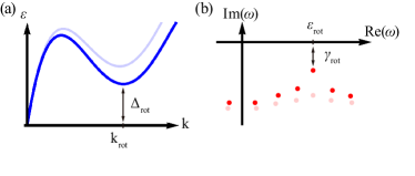
Figure 1: Soft modes before the transition to (a) spatial crystals and (b) time crystals. (a) The excitation spectrum with a roton structure in a quantum liquid near the transition to a spatial crystal. (b) The poles of the response function in an open quantum system on the complex plane near the transition to a time crystal.

In this paper, we generalize the concept of roton mode softening mechanism to time crystalline transitions in open quantum systems. We use a modified dissipative Dicke model as a prototypical example. This model exhibits a CTC order when the atom-photon coupling is time-independent; while it can enter a DTC phase as the atom-photon coupling is driven periodically. Using the Keldysh formalism, we study Gaussian fluctuations in the normal phase near the transitions to the CTC and DTC phase. We found that the photon response function, $\chi_{\mathrm{ph}}\left(\omega\right)$ diverges at a finite frequency $\omega=\varepsilon_{\mathrm{rot}}$ on approaching the time crystalline transitions. This divergence is controlled by the softening of the relaxation rate of a collective excitation $\gamma_{\mathrm{rot}}\rightarrow 0$, while keeping the excitation frequency to be finite, $\varepsilon_{\mathrm{rot}}>0$, during the transition. This frequency $\varepsilon_{\mathrm{rot}}$ plays the role of the roton momentum $\mathbf{k}_{\mathrm{rot}}$ in spatial crystals, which determines the corresponding period of the time crystalline orders; while $\gamma_{\mathrm{rot}}$ plays the role of roton gap $\Delta_{\mathrm{rot}}$, which vanishes at the transition and leads the normal phase to be unstable. The comparison of the mode softening mechanisms in spatial crystals and time crystals is given in Table.1 and Fig.1. This softening mechanism can be clearly seen by the poles of the response function on the complex plane, where the poles will cross the real axis at $\varepsilon_{\mathrm{rot}}$ during the transition, see Fig.1. Using this ”roton softening” analysis, we predict a time quasi-crystal phase in our model, in which the self-organized period and the driving period are incommensurate Autti et al. (2018); Giergiel et al. (2019).

This paper is organized as follows. We first introduced the modified Dicke model in Sec. II. Then, we study the phase diagram in the case of a constant atom-cavity coupling and discuss the mode softening in the continuous time crystal by Gaussian fluctuation and exact diagonalization in Sec. III. In Sec. IV, we consider the atom-cavity coupling to be periodically driven, and demonstrate the mode softening in the discrete time crystal and the time quasi-crystal. We summarize with a discussion in Sec. V.

Table 1: Comparison of the mode softening mechanisms in spatial crystals and time crystals.

	Spatial crystals	Time crystals
Inverse period	finite $\mathbf{k}_{\mathrm{rot}}$	finite $\varepsilon_{\mathrm{rot}}$
Mode softening	$\Delta_{\mathrm{rot}}\to 0$	$\gamma_{\mathrm{rot}}\to 0$
Divergence of response	$\chi(\mathbf{k}=\mathbf{k}_{\mathrm{rot}},\omega=0)\to\infty$	$\chi(\omega=\varepsilon_{\mathrm{rot}})\to\infty$

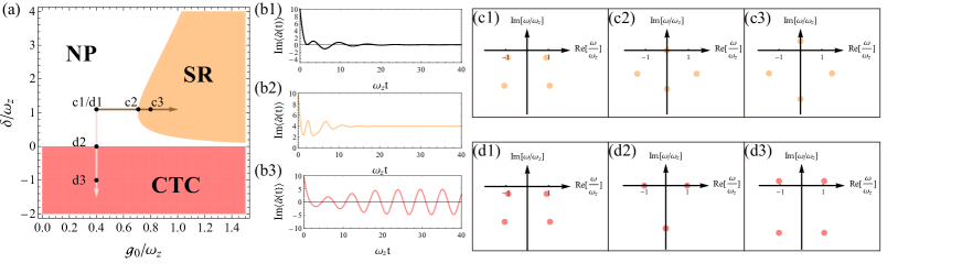
Figure 2: (a) Phase diagram obtained by solving saddle point equations (11,12) with parameters $\kappa/\omega_{z}=1$ and $U/(N\omega_{z})=0.01$. (b) Long-time dynamics of three different phases. (b1) The normal phase (NP), in which the photon number vanishes after a sufficiently long time. (b2) The superradiant phase (SR), in which the system reaches a steady state with finite photon occupation. (b3) The continuous time crystal phase (CTC). The cavity field oscillates periodically over time and has no steady state. (c)(d) Poles of the response function on the complex plane. The corresponding parameters are given by the points (c1,c2,c3) and (d1,d2,d3) in the phase diagram Fig.2(a).

II Model

We consider a modified dissipative Dicke model, which describes the interaction between $N$ two-level atoms and a single cavity mode Keeling et al. (2010); Bhaseen et al. (2012). The Hamiltonian takes the following form ($\hbar=1$),

$$\hat{H} = \omega_{0}\hat{a}^{\dagger}\hat{a}+\sum_{i=1}^{N}\frac{\omega_{z}}{2}\hat{\sigma}_{i}^{z}$$ (1)

$$+\sum_{i=1}^{N}\frac{g(t)}{\sqrt{N}}\left(\hat{a}+\hat{a}^{\dagger}\right)\hat{\sigma}_{i}^{x}+\sum_{i=1}^{N}\frac{U}{2N}\hat{a}^{\dagger}\hat{a}\hat{\sigma}_{i}^{z},$$

where $\hat{a}$, $\hat{a}^{\dagger}$ are the annihilation and creation operators of cavity photons, and $\hat{\sigma}_{i}^{\alpha}$ with $\alpha=x,y,z$ are Pauli matrices describing two-level atoms. The cavity frequency is $\omega_{0}$, level splitting of the atom is $\omega_{z}$, $g(t)$ is the atom-photon coupling, and $N$ is the total atom number. The interaction $U$ can be regarded as a Stark shift of atomic levels in the cavity field. In the work, we only consider the situation of $U>0$. Besides the coherent process governed by the Hamiltonian (1), leaking of cavity photons leads to dissipative dynamics. Thus the system can be described by a Lindblad equation $\partial_{t}\hat{\rho}=-i\left[H,\hat{\rho}\right]+\kappa\left(2\hat{a}\hat{\rho}\hat{a}^{\dagger}-\left\{\hat{\rho},\hat{a}^{\dagger}\hat{a}\right\}\right)$, where $\kappa$ is the photon loss rate.

We introduce a collective spin of atoms as $\hat{\mathbf{S}}=\frac{1}{2}\sum_{i=1}^{N}\hat{\mathbf{\sigma}}_{i}$. the Hamiltonian can be written into

$$\hat{H} = \omega_{0}\hat{a}^{\dagger}\hat{a}+\omega_{z}\hat{S}_{z}+\frac{U}{N}\hat{a}^{\dagger}\hat{a}\hat{S}^{z}$$ (2)

$$+\frac{2g(t)}{\sqrt{N}}\left(\hat{a}+\hat{a}^{\dagger}\right)\hat{S}^{x}.$$

A Holstein-Primakoff transformation is performed, such that the collective spin can be expressed by bosons, $\hat{S}_{z}=\hat{b}^{\dagger}\hat{b}-N/2$ and $\hat{S}^{+}=\hat{S}_{x}+i\hat{S}_{y}=\hat{b}^{\dagger}\sqrt{N-\hat{b}^{\dagger}\hat{b}}.$ Then we expand the Hamiltonian (1) to the order of $O(1/N)$ as

$$\hat{H} \approx \delta\hat{a}^{\dagger}\hat{a}+\omega_{z}\hat{b}^{\dagger}\hat{b}+g(t)\left(\hat{a}+\hat{a}^{\dagger}\right)\left(\hat{b}+\hat{b}^{\dagger}\right)$$ (3)

$$-\frac{g(t)}{2N}\left(\hat{a}+\hat{a}^{\dagger}\right)\hat{b}^{\dagger}\left(\hat{b}+\hat{b}^{\dagger}\right)\hat{b}+\frac{U}{N}\hat{a}^{\dagger}\hat{a}\hat{b}^{\dagger}\hat{b},$$

where $\delta=\omega_{0}-U/2$.

To investigate the non-equilibrium dynamics, we employ the Keldysh path integral approach of open quantum systems Torre et al. (2013); Sieberer et al. (2016). The Keldysh path integral is equivalent to the Lindblad master equation of the density matrix. As we know the density matrix can be acted on from both sides, thus there are a time-forward($+$) and a time-backward($-$) components of the fields in the Keldysh formalism Sieberer et al. (2016). By doing the path-integral in the basis of coherent states on the two time branches, bosonic operators are replaced by time-dependent complex-valued fields. The Keldysh partition function is given by

$$Z=\int\mathcal{D}\left[a_{+}^{\ast},a_{+},a_{-}^{\ast},a_{-},b_{+}^{\ast},b_{+},b_{-}^{\ast},b_{-}\right]e^{iS},$$ (4)

and the Keldysh action is

$$S = \int_{t}\{a_{+}^{\ast}i\partial_{t}a_{+}+b_{+}^{\ast}i\partial_{t}b_{+}-H_{+}$$ (5)

$$-a_{-}^{\ast}i\partial_{t}a_{-}-b_{-}^{\ast}i\partial_{t}b_{-}+H_{-}$$

$$-i\kappa\left(2a_{+}a_{-}^{\ast}-a_{+}^{\ast}a_{+}-a_{-}^{\ast}a_{-}\right)\},$$

in which $H_{\pm}$ is given by

$$H_{\pm} = \delta{a}_{\pm}^{\ast}{a}_{\pm}+\omega_{z}{b}_{\pm}^{\ast}{b}_{\pm}+g(t)\left({a}_{\pm}+{a}_{\pm}^{\ast}\right)\left({b}_{\pm}+{b}_{\pm}^{\ast}\right)$$ (6)

$$-\frac{g(t)}{2N}\left({a}_{\pm}+{a}_{\pm}^{\ast}\right){b}_{\pm}^{\ast}\left({b}_{\pm}+{b}_{\pm}^{\ast}\right){b}_{\pm}$$

$$+\frac{U}{N}{a}_{\pm}^{\ast}{a}_{\pm}{b}_{\pm}^{\ast}{b}_{\pm}.$$

Then we apply the Keldysh rotation, $\psi_{\mathrm{cl}}=\left(\psi_{+}+\psi_{-}\right)/\sqrt{2},\psi_{\mathrm{q}}=(\psi_{+}-\psi_{-})/\sqrt{2}$, where $\psi=a,b$. The index $\mathrm{cl}(\mathrm{q})$ stands for the ’classical’ (’quantum’) part of fields. These fields are named ’classical’ and ’quantum’, only because the former can acquire an finite expectation value while the latter cannot. It does not indicate the ’classical’ field can not fluctuate.

In this new basis, we write the total action into $S=S_{2}+S_{4}/N$. Here $S_{2}$ is the quadratic action given by

$$S_{2} = \int_{t}\left(a_{\mathrm{cl}}^{\ast},a_{\mathrm{q}}^{\ast}\right)\begin{pmatrix}0&i\partial_{t}-\delta-i\kappa\\ i\partial_{t}-\delta+i\kappa&2i\kappa\end{pmatrix}\begin{pmatrix}a_{\mathrm{cl}}\\ a_{\mathrm{q}}\end{pmatrix}$$ (7)

$$+\int_{t}\left(b_{\mathrm{cl}}^{\ast},b_{\mathrm{q}}^{\ast}\right)\begin{pmatrix}0&i\partial_{t}-\omega_{z}\\ i\partial_{t}-\omega_{z}&0\end{pmatrix}\begin{pmatrix}b_{\mathrm{cl}}\\ b_{\mathrm{q}}\end{pmatrix}$$

$$-4g(t)\int_{t}\left[\mathrm{Re}\left(a_{\mathrm{cl}}\right)\mathrm{Re}\left(b_{\mathrm{q}}\right)+\mathrm{Re}\left(a_{\mathrm{q}}\right)\mathrm{Re}\left(b_{\mathrm{cl}}\right)\right],$$

and the quartic term $S_{4}$ is

$$S_{4} = \frac{g}{2}\int_{t}\left[\mathrm{Re}\left(a_{\mathrm{cl}}+a_{\mathrm{q}}\right)\mathrm{Re}\left(b_{\mathrm{cl}}+b_{\mathrm{q}}\right)\left|b_{\mathrm{cl}}+b_{\mathrm{q}}\right|^{2}\right.$$ (8)

$$\left.-\mathrm{Re}\left(a_{\mathrm{cl}}-a_{\mathrm{q}}\right)\mathrm{Re}\left(b_{\mathrm{cl}}-b_{\mathrm{q}}\right)\left|b_{\mathrm{cl}}-b_{\mathrm{q}}\right|^{2}\right]$$

$$-\frac{U}{4}\int_{t}\left[\left|a_{\mathrm{cl}}+a_{\mathrm{q}}\right|^{2}\left|b_{\mathrm{cl}}+b_{\mathrm{q}}\right|\right.^{2}$$

$$\left.-\left|a_{\mathrm{cl}}-a_{\mathrm{q}}\right|^{2}\left|b_{\mathrm{cl}}-b_{\mathrm{q}}\right|^{2}\right].$$

Apply the saddle point approximation Sieberer et al. (2016),

$$0 = \left.\frac{\delta S}{\delta a_{\mathrm{q}}^{\ast}}\right|_{a_{\mathrm{q}}=b_{\mathrm{q}}=0},$$ (9)

$$0 = \left.\frac{\delta S}{\delta b_{\mathrm{q}}^{\ast}}\right|_{a_{\mathrm{q}}=b_{\mathrm{q}}=0},$$ (10)

we obtain

$$i\frac{\partial a_{\mathrm{cl}}}{\partial t} = \left(\delta-i\kappa+\frac{U\left|b_{\mathrm{cl}}\right|^{2}}{2N}\right)a_{\mathrm{cl}}$$ (11)

$$\,+2g\left(t\right)\left(1-\frac{\left|b_{\mathrm{cl}}\right|^{2}}{4N}\right)\mathrm{Re}\left(b_{\mathrm{cl}}\right),$$

$$i\frac{\partial b_{\mathrm{cl}}}{\partial t} = \left(\omega_{z}+\frac{U\left|a_{\mathrm{cl}}\right|^{2}}{2N}\right)b_{\mathrm{cl}}$$ (12)

$$\,+2g\left(t\right)\left(1-\frac{b_{\mathrm{cl}}\left(b_{\mathrm{cl}}+2b_{\mathrm{cl}}^{\ast}\right)}{4N}\right)\mathrm{Re}\left(a_{\mathrm{cl}}\right).$$

Setting $a_{\mathrm{cl}}\left(t\right)=\sqrt{2}\left\langle\hat{a}\left(t\right)\right\rangle$ and $b_{\mathrm{cl}}\left(t\right)=\sqrt{2}\left\langle\hat{b}\left(t\right)\right\rangle$, one could reproduce the usual mean-field equations of motion, which can describe the colletive dynamics of this open Dicke model Keeling et al. (2010); Bhaseen et al. (2012).

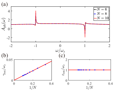
Figure 3: (a) Photon spectral functions at $\delta=0$ for finite $N$, in which $\kappa/\omega_{z}=3,g_{0}/\omega_{z}=0.3,$ and $U/\omega_{z}=0.1$. (b)(c) Finite-size scaling of the damping rate $\gamma_{\mathrm{rot}}$ and frequency $\varepsilon_{\mathrm{rot}}$ respectively. The damping rate is obtained by the full width at half maximum of the peaks, and the frequency is obtained by the position of the peaks. The blue dots are the numerical data, and the solid red line is a linear fitting.

III Mode softening in the continuous time crystal

We first investigate the long-time dynamics for a time-independent atom-cavity coupling strength $g(t)=g_{0}$. In this situation, the Lindblad master equation has a continuous time translation symmetry. We obtain the phase diagram by solving the saddle point equations (11,12), see Fig.2(a). There are three different non-equilibrium phases. When $\delta>0$, there is a well-known superradiant transition at $g_{\ast}=\sqrt{\frac{\delta^{2}+\kappa^{2}}{4\delta}\omega_{z}}$. If $g_{0}<g_{\ast}$, the system will reach a steady normal phase (NP) after a sufficiently long time with an empty cavity, $\left\langle\hat{a}\left(t\right)\right\rangle=0$ (Fig.2(b1)). As $g_{0}$ exceeds $g_{*}$, the system will enter a steady superradiant phase (SR). In this phase the cavity photons condense so that $\left\langle\hat{a}\left(t\right)\right\rangle\neq 0$, see Fig.2(b2). In the region of $\delta<0$, no steady states are found. Instead, the system will develop a CTC order. Both the cavity $\left\langle\hat{a}\left(t\right)\right\rangle$ and atoms $\left\langle\hat{b}\left(t\right)\right\rangle$ show permanent periodical oscillations in this phase (Fig.2(b3)). These oscillations are robust against external perturbations Bhaseen et al. (2012)(and see Appendix A). It breaks the continuous time translation symmetry of the Lindblad equation. In the limit of $\left|\delta\right|/U\ll 1$, the oscillations are approximately harmonic,

$$\left\langle\hat{a}\left(t\right)\right\rangle \approx \frac{2ig_{0}}{\sqrt{\omega_{z}^{2}+\kappa^{2}}}\sqrt{\frac{N\left|\delta\right|}{U}}\cos\left(\varepsilon t\right),$$ (13)

$$\left\langle\hat{b}\left(t\right)\right\rangle \approx -\sqrt{\frac{N\left|\delta\right|}{U}}e^{-i\left(\varepsilon t+\phi\right)},$$ (14)

where $\varepsilon=\omega_{z}+2\left|\delta\right|g_{0}^{2}/\left(\omega_{z}^{2}+\kappa^{2}\right)$, and $\cos\phi=\kappa/\sqrt{\varepsilon^{2}+\kappa^{2}}$.

To investigate mode softening during phase transitions, we consider quantum fluctuations beyond saddle point approximation. First, we keep the action to quadratic terms above the saddle point of the normal phase Torre et al. (2013). It gives $S\approx S_{2}$. Note that in the thermodynamic limit $N\rightarrow\infty$, $1/N$ terms can be ignored and this expansion is exact. Here we define a Nambu spinor as $\Psi_{\lambda}(\omega)=\left(a_{\lambda}(\omega),a_{\lambda}^{\ast}(-\omega),b_{\lambda}(\omega),b_{\lambda}^{\ast}(-\omega)\right)^{\mathrm{T}}$ in frequency domain. $\lambda=\mathrm{cl,q}$, for classical and quantum components. The quadratic action then can be expressed into a compact form,

$$S_{2} = \frac{1}{2}\int_{\omega}\left(\Psi_{\mathrm{cl}}^{{\dagger}}(\omega),\Psi_{\mathrm{q}}^{{\dagger}}(\omega)\right)M_{0}(\omega)\binom{\Psi_{\mathrm{cl}}(\omega)}{\Psi_{\mathrm{q}}(\omega)},$$ (15)

where

$$M_{0}(\omega)=\begin{pmatrix}0&\left[G_{0}^{\mathrm{A}}\right]^{-1}(\omega)\\ \left[{G_{0}^{\mathrm{R}}}\right]^{-1}(\omega)&D_{0}^{\mathrm{K}}(\omega)\end{pmatrix}$$ (16)

and

$$\left[G_{0}^{\mathrm{R}}\right]^{-1}(\omega)=$$ (17)

$$\begin{pmatrix}\omega-\delta+i\kappa&0&-g_{0}&-g_{0}\\ 0&-\omega-\delta-i\kappa&-g_{0}&-g_{0}\\ -g_{0}&-g_{0}&\omega-\omega_{z}&0\\ -g_{0}&-g_{0}&0&-\omega-\omega_{z}\end{pmatrix},$$

$$\left[{G_{0}^{\mathrm{A}}}\right]^{-1}(\omega)=\left(\left[{G_{0}^{\mathrm{R}}}\right]^{-1}(\omega)\right)^{{\dagger}},$$ (18)

$$D_{0}^{\mathrm{K}}(\omega)=2i\kappa\mathrm{diag}\left(1,1,0,0\right).$$ (19)

The retarded/advanced/Keldysh Green’s functions can be obtained by

$$\begin{pmatrix}G_{0}^{\mathrm{K}}(\omega)&G_{0}^{\mathrm{R}}(\omega)\\ G_{0}^{\mathrm{A}}(\omega)&0\end{pmatrix}=M_{0}(\omega)^{-1}.$$ (20)

One seeks the poles of the retarded Green’s function by solving $\det[{G_{0}^{\mathrm{R}}}(\omega)]^{-1}=0$. Due to the particle-hole symmetry of Nambu space $\left(\sigma_{x}\otimes I\right)[{G_{0}^{\mathrm{R}}}(-\omega^{\ast})]^{-1}\left(\sigma_{x}\otimes I\right)=\left[{G_{0}^{\mathrm{R}}}(\omega)\right]^{-1\ast}$, the poles must come in symmetric pairs about the imaginary axis, see Fig.2(c,d). The real parts of the poles are the energies of collective modes. The imaginary parts represent the relaxation rates of these modes and must be negative. That is to say, the poles should be always in the lower half complex plane. When a pole happens to appear in the upper half complex plane, it implies that an excitation mode will be exponentially amplified in evolution. That will make the system unstable, and a corresponding phase transition is about to take place.

We analyze trajectories of the poles of response function on the complex plane near the phase transitions. We found that the superradiant phase transition and the time crystalline transition occur in fundamentally different ways. Near the superradiant transition, as $g_{0}\rightarrow g_{\ast}$ (see trajectory c1-c2-c3 in Fig.2(a)), a pair of poles will first move to the imaginary axis, which indicates the vanishing of excitation energy. After meeting each other on the imaginary axis, this pair of poles will split in the imaginary direction. Near the transition, one pole is near the axis origin,

$$\omega\approx 2i\sqrt{\frac{\delta(\kappa^{2}+\delta^{2})}{\omega_{z}\kappa^{2}}}(g_{0}-g_{*}).$$ (21)

When $g_{0}=g_{\ast}$, the upper one of the poles will cross the real axis at $\omega=0$, such that the imaginary part changes its sign to positive Torre et al. (2013), see Fig.2(c). That leads to a transition to a steady superradiant phase. Of course, after the transition, quantum fluctuations above the saddle point of the normal phase become unstable, and one should analyze the fluctuations around a correct saddle point, i.e. the superradiant saddle point.

In the other case, in the vicinity of the time crystalline transition ($\delta\rightarrow 0^{+}$), there are a pair of poles near the real axis, see Fig.2(d), $\omega=\pm\varepsilon_{\mathrm{rot}}-i\gamma_{\mathrm{rot}}$, where

$$\varepsilon_{\mathrm{rot}} \approx \omega_{z}+\frac{2g_{0}^{2}\left(\omega_{z}^{2}-\kappa^{2}\right)}{\left(\omega_{z}^{2}+\kappa^{2}\right)^{2}}\delta,$$ (22)

$$\gamma_{\mathrm{rot}} \approx \frac{4g_{0}^{2}\omega_{z}\kappa}{\left(\omega_{z}^{2}+\kappa^{2}\right)^{2}}\delta.$$ (23)

These two poles dominate the photon’s response function in the long time limit, $\chi_{\mathrm{ph}}(\omega)=-i\int\mathrm{d}t\,e^{i\omega t}\theta(t)\left\langle\left[\hat{a}(t),\hat{a}^{\dagger}(0)\right]\right\rangle$. It can be calculated by the first diagonal element of the retarded Green’s function matrix $G_{0}^{\mathrm{R}}(\omega)$ as

$$\chi_{\mathrm{ph}}(\omega)\sim\frac{2\left(\omega+i\gamma_{\mathrm{rot}}\right)}{\left(\omega+i\gamma_{\mathrm{rot}}\right)^{2}-\varepsilon_{\mathrm{rot}}^{2}}.$$ (24)

Note that as $\delta\rightarrow 0^{+}$, these two poles approach the real axis, $\gamma_{\mathrm{rot}}\rightarrow 0$, but their real parts remain finite $\varepsilon_{\mathrm{rot}}\rightarrow\omega_{z}$. At the transition, the poles cross the real axis at $\omega=\pm\omega_{z}$ instead of $\omega=0$ in superradiant transition. Thus the response function will diverge at finite frequencies Scarlatella et al. (2019), $\left|{\chi_{\mathrm{{ph}}}}(\pm\omega_{z})\right|\sim 1/\gamma_{\mathrm{rot}}\sim 1/\left|\delta\right|$. As a consequence, a time crystalline phase emerges and the system will oscillate at $\pm\omega_{z}$, right after the transition. That is consistent with the previous saddle point solution (13,14). We further calculate the photon correlation function, corresponding to the first diagonal element of the Keldysh Green’s function matrix $G_{0}^{\mathrm{K}}(\omega)$, obtaining

$$C_{\mathrm{ph}}(t) = \left\langle\left\{\hat{a}\left(t\right),\hat{a}^{\dagger}\left(0\right)\right\}\right\rangle$$ (25)

$$\approx \frac{g_{0}^{2}}{\omega_{z}\delta}\cos\left(\varepsilon_{\mathrm{rot}}t\right)e^{-\gamma_{\mathrm{rot}}\left|t\right|}$$

near the transition. Note that both the photon number $\left\langle\hat{a}^{\dagger}\hat{a}\right\rangle=\left[C_{\mathrm{ph}}(0)-1\right]/2=\frac{g_{0}^{2}-\omega_{z}\delta}{2\omega_{z}\delta}$ and the relaxation time $1/\gamma_{\mathrm{rot}}$ diverge with exponent $\nu=1$.

To go beyond the Gaussian fluctuation, we numerically diagonalize the Lindblad equation for a finite atomic number $N$ at the transition point $\delta=0$, and make a finite-size scaling analysis. We obtain the photon spectral function, $A_{\mathrm{ph}}(\omega)=-2\mathrm{Im}\chi_{\mathrm{ph}}(\omega)$. The spectral functions of different numbers of atoms $N$ are plotted in Fig.3(a). This spectral function exhibits two peaks around $\omega=\pm\omega_{z}$. We abstract the damping rate $\gamma_{\mathrm{rot}}$ and excitation energy $\varepsilon_{\mathrm{rot}}$ from the width and the position of the peaks respectively. Then we make a finite-size scaling. The results are plotted in Fig.3(b). Note that for a finite atom number $N$, damping rate $\gamma_{\mathrm{rot}}$ is finite at $\delta=0$. As $N$ increase, $\gamma_{\mathrm{rot}}$ will approach zero. At the same time, $\varepsilon_{\mathrm{rot}}$ will remain $\omega_{z}$ as $N\rightarrow\infty$. That is consistent with our analysis of Gaussian fluctuation.

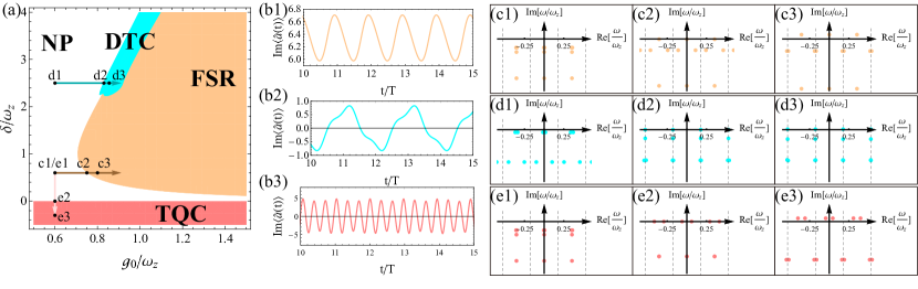
Figure 4: (a) Phase diagram of the periodically driven case, obtained by solving saddle point equations (11,12) with parameters $\kappa/\omega_{z}=1$, $g_{1}/\omega_{z}=0.05$, $U/(N\omega_{z})=0.01$ and $\Omega/\omega_{z}=\frac{\sqrt{2}}{4}\approx 0.353$. (b) Long-time dynamics of three different phases. (b1) The Floquet superradiant phase (FSR), in which the system oscillates with driving period $T$. (b2) The discrete time crystal phase (DTC), where the period is doubled, $2T$. (b3) The time quasi-crystal phase (TQC). (c)(d)(e) Poles of the response function on the complex plane. The dashed lines represent the boundary of Floquet-Brillouin zone. The corresponding parameters are given by the points (c1,c2,c3), (d1,d2,d3) and (e1,e2,e3), in the phase diagram Fig.4(a)

IV Mode softening in the discrete time crystal and the time quasi-crystal

In the following, we will demonstrate our mode softening analysis can also be applied to discrete time crystalline transitions. We modulate the atom-photon coupling strength periodically $g\left(t\right)=g_{0}+g_{1}\cos\left(\Omega t\right)$. In this situation, the Lindblad equation is invariant only under a discrete time translation with period $T=2\pi/\Omega$. By solving the corresponding saddle point equations (11,12), we found three different phases at $\delta>0$, see Fig.4(a). When $g_{0}$ is small, the cavity reaches a steady NP after a sufficiently long time $\left\langle\hat{a}(t)\right\rangle=0$. When $g_{0}$ is sufficiently large, the system approaches a Floquet superradiant phase (FSR), in which the cavity field is nonzero and oscillates with the driving period, see Fig.4(b1). Between the NP and the FSR, a DTC phase is found, in which the oscillation period is doubled (Fig.4(b2)), thereby breaking the discrete time translation symmetry.

As before, we consider Gaussian fluctuations in the NP. In contrast to the undriven case, we obtain infinite poles on the complex plane Mathey and Diehl (2019, 2020), see in Fig.4(c,d,e). For a periodic potential, different momentum components separated by the reciprocal vector are coupled due to lattice scattering. Quasi-momentum defined in the first Brillouin zone is a good quantum number. Similarly, different frequency components of the same quasi-energy are coupled in our mono-chromatically driven system, the action expressed in the frequency domain is tri-diagonal,

$$S_{2} = \frac{1}{2}\int_{-\frac{\Omega}{2}}^{\frac{\Omega}{2}}\mathrm{d}\omega\,\begin{pmatrix}\cdots&\Psi(\omega)^{\dagger},&\Psi(\omega+\Omega)^{\dagger}&\cdots\end{pmatrix}\begin{pmatrix}\ddots&\ddots&&\\ \ddots&M_{0}(\omega)&M_{1}&\\ &M_{1}&M_{0}(\omega+\Omega)&\ddots\\ &&\ddots&\ddots\\ \end{pmatrix}\begin{pmatrix}\vdots\\ \Psi(\omega)\\ \Psi(\omega+\Omega)\\ \vdots\end{pmatrix}.$$ (26)

where

$$M_{1}=\begin{pmatrix}0&\left[G_{1}^{\mathrm{A}}\right]^{-1}\\ \left[{G_{1}^{\mathrm{R}}}\right]^{-1}&0\end{pmatrix},$$ (27)

and

$$\left[{G_{1}^{\mathrm{R}}}\right]^{-1}=\left[{G_{1}^{\mathrm{A}}}\right]^{-1}=\frac{1}{2}\begin{pmatrix}0&0&-g_{1}&-g_{1}\\ 0&0&-g_{1}&-g_{1}\\ -g_{1}&-g_{1}&0&0\\ -g_{1}&-g_{1}&0&0\end{pmatrix}.$$ (28)

Such that the dimension of the retarded Green’s function $G^{\mathrm{R}}\left(\omega\right)$ is infinite rather than $4\times 4$ in the undriven case

$$\left[{G^{\mathrm{R}}(\omega)}\right]^{-1}=\begin{pmatrix}\ddots&\ddots&&&\\ \ddots&\left[{G_{0}^{\mathrm{R}}(\omega-\Omega)}\right]^{-1}&\left[{G_{1}^{\mathrm{R}}}\right]^{-1}&&\\ &\left[{G_{1}^{\mathrm{R}}}\right]^{-1}&\left[{G_{0}^{\mathrm{R}}(\omega)}\right]^{-1}&\left[{G_{1}^{\mathrm{R}}}\right]^{-1}&\\ &&\left[{G_{1}^{\mathrm{R}}}\right]^{-1}&\left[{G_{0}^{\mathrm{R}}(\omega+\Omega)}\right]^{-1}&\ddots\\ &&&\ddots&\ddots\\ \end{pmatrix},$$ (29)

To calculate the poles of the retarded Green’s function numerically, we have to make a dimensional cutoff. In practice, we take 19 Floquet-Brillouin zones into account, i.e. the matrix size is 76$\times$76. Poles manifest perfect periodicity in the five Brillouin Zones nearest to zero and are convergent with growing cutoff size, which means our cutoff is sufficiently large.

The real parts of the poles are equally spaced by $\Omega$. At the transition to the FSR phase, a chain of poles will cross the real axis at the center of the Floquet-Brillouin zones, $\omega=n\Omega$, see Fig.4(c). That means the oscillation period of the upcoming FSR is just the driving period $T$. When approaching the DTC transition, see Fig.4(c), the chains poles will cross the real axis at the boundary of Floquet-Brillouin zones, $\omega=\left(n+1/2\right)\Omega$. The photon’s response function will diverge at these frequencies, $\omega=\left(n+1/2\right)\Omega$. As a consequence of this mode softening, the oscillation period is doubled after the transition.

When $\delta\rightarrow 0$, we found that the poles will cross the real axis at $\pm\omega_{z}+n\Omega$. According to our mode softening analysis, a time crystalline order may emerge at frequency $\pm\omega_{z}+n\Omega$. If the external driving frequency $\Omega$ and the intrinsic energy $\omega_{z}$ are incommensurate, the oscillation will become quasi-periodic. That is to say, a time quasi-crystal(TQC) may emerge in the $\delta<0$ regime. Thus we numerically solve the saddle point equations in this regime and plot the long-time evolution in Fig.4(b3). Note that the oscillation is quasi-periodic and will not repeat itself in a finite time. This numerical result is consistent with our mode softening analysis. The robustness of the DTC and the TQC against perturbations is checked in Appendix A.

V Summary and Outlooks

We generalize the ”roton” mode softening mechanism of spatial crystals to time crystals in open quantum systems. In time crystalline transition, the softening mechanism is that the damping rate of a collective mode will vanish, while the energy of this mode remains finite. That indicates the emergence of an undamped mode with non-zero energy in open systems, which will compete with the existing steady state, leading to the possible order in the time domain.

In experiments, the Dicke model discussed in this work can be regarded as a simplified mode of the current experiments Kongkhambut et al. (2022); Zupancic et al. (2019). The two internal atomic levels are simulated by the center-of-mass states of atoms, and the coupling $g$ can be tuned via modulating the transversal pumping laser. The response of atoms can be measured by a Bragg-like probe Mottl et al. (2012), and the correlations of the cavity field can be obtained by measuring the photons leaking out of the cavity Keßler et al. (2021). We expect that this mode softening in time crystals can be observed in those experiments.

In this work, our discussion is limited in open quantum systems. The damping of collective modes is dominated by external dissipation. However, this mode softening mechanism can be also generalized to closed systems, where the relaxation is induced by multi-mode couplings.

Acknowledgment. We thank Hui Zhai, Zheyu Shi and Junsen Wang for helpful discussions.

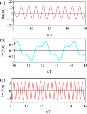
Figure 5: Photon dynamics under perturbation in the generalized Dicke model. (a)The CTC phase, (b)The DTC phases and (c) the time quasi-crystal phase. Here $\delta g/g=0.1$ and the driving frequency is tuned to be $\Omega^{\prime}/\omega_{z}=\sqrt{2}/5$.

Appendix A Robustness of the Dicke Time Crystals

Time crystals are robust against perturbations. In this appendix, We will show the time crystal phases, including CTC, DTC and time quasi-crystal, are robust against adding perturbation and changing parameters. We add a perturbation like $\frac{2\delta g}{i\sqrt{N}}(\hat{a}-\hat{a}^{\dagger})\hat{S}_{y}$ into the Hamiltonian 2. This perturbation appears as the rotating-wave term and antirotating-wave term of the atom-light coupling are tuned imbalanced. Then we consider the saddle point solutions with $\delta g/g=0.1$, and investigate the sufficient long time behavior. We found that the CTC phase is robust against the perturbation, see Fig.5(a).

For the periodically driven case, we remain the unbalanced perturbation $\delta g/g=0.1$, and tune the driving period to be $\Omega^{\prime}/\omega_{z}=\sqrt{2}/5$. In the DTC phase, the system oscillates with a doubled period of driving, $T^{\prime}=2\pi/\Omega^{\prime}$, see Fig.5(b). Besides, the system will again enter the time quasi-crystal phase, when $\delta<0$ (Fig.5(c)). That indicates the both DTC and time quasi-crystal are robust against such perturbation.

References

- Henshaw and Woods (1961) D. G. Henshaw and A. D. B. Woods, Phys. Rev. 121, 1266 (1961).
- Griffin (1993) A. Griffin, Excitations in a Bose-Condensed Liquid, Cambridge Studies in Low Temperature Physics (Cambridge University Press, Cambridge, 1993).
- Zheng and Li (2012) W. Zheng and Z. Li, Phys. Rev. A 85, 053607 (2012).
- Martone et al. (2012) G. I. Martone, Y. Li, L. P. Pitaevskii, and S. Stringari, Phys. Rev. A 86, 063621 (2012).
- Khamehchi et al. (2014) M. A. Khamehchi, Y. Zhang, C. Hamner, T. Busch, and P. Engels, Phys. Rev. A 90, 063624 (2014).
- Ji et al. (2015) S.-C. Ji, L. Zhang, X.-T. Xu, Z. Wu, Y. Deng, S. Chen, and J.-W. Pan, Phys. Rev. Lett. 114, 105301 (2015).
- Ha et al. (2015) L.-C. Ha, L. W. Clark, C. V. Parker, B. M. Anderson, and C. Chin, Phys. Rev. Lett. 114, 055301 (2015).
- Santos et al. (2003) L. Santos, G. V. Shlyapnikov, and M. Lewenstein, Phys. Rev. Lett. 90, 250403 (2003).
- O’Dell et al. (2003) D. H. J. O’Dell, S. Giovanazzi, and G. Kurizki, Phys. Rev. Lett. 90, 110402 (2003).
- Henkel et al. (2010) N. Henkel, R. Nath, and T. Pohl, Phys. Rev. Lett. 104, 195302 (2010).
- Chomaz et al. (2018) L. Chomaz, R. M. W. van Bijnen, D. Petter, G. Faraoni, S. Baier, J. H. Becher, M. J. Mark, F. Wächtler, L. Santos, and F. Ferlaino, Nature Phys 14, 442 (2018).
- Mottl et al. (2012) R. Mottl, F. Brennecke, K. Baumann, R. Landig, T. Donner, and T. Esslinger, Science 336, 1570 (2012).
- Wilczek (2012) F. Wilczek, Phys. Rev. Lett. 109, 160401 (2012).
- Shapere and Wilczek (2012) A. Shapere and F. Wilczek, Phys. Rev. Lett. 109, 160402 (2012).
- Bruno (2013) P. Bruno, Phys. Rev. Lett. 111, 070402 (2013).
- Watanabe and Oshikawa (2015) H. Watanabe and M. Oshikawa, Phys. Rev. Lett. 114, 251603 (2015).
- Sacha (2015) K. Sacha, Phys. Rev. A 91, 033617 (2015).
- Else et al. (2016) D. V. Else, B. Bauer, and C. Nayak, Phys. Rev. Lett. 117, 090402 (2016).
- Khemani et al. (2016) V. Khemani, A. Lazarides, R. Moessner, and S. L. Sondhi, Phys. Rev. Lett. 116, 250401 (2016).
- von Keyserlingk and Sondhi (2016) C. W. von Keyserlingk and S. L. Sondhi, Phys. Rev. B 93, 245146 (2016).
- Yao et al. (2017) N. Y. Yao, A. C. Potter, I.-D. Potirniche, and A. Vishwanath, Phys. Rev. Lett. 118, 030401 (2017).
- Else et al. (2017) D. V. Else, B. Bauer, and C. Nayak, Phys. Rev. X 7, 011026 (2017).
- Sacha and Zakrzewski (2018) K. Sacha and J. Zakrzewski, Rep. Prog. Phys. 81, 016401 (2018).
- Else et al. (2020) D. V. Else, C. Monroe, C. Nayak, and N. Y. Yao, Annu. Rev. Condens. Matter Phys. 11, 467 (2020).
- Yang and Cai (2021) X. Yang and Z. Cai, Phys. Rev. Lett. 126, 020602 (2021).
- Gambetta et al. (2019) F. M. Gambetta, F. Carollo, M. Marcuzzi, J. P. Garrahan, and I. Lesanovsky, Phys. Rev. Lett. 122, 015701 (2019).
- Yue et al. (2022) M. Yue, X. Yang, and Z. Cai, Phys. Rev. B 105, L100303 (2022).
- Zhang et al. (2017) J. Zhang, P. W. Hess, A. Kyprianidis, P. Becker, A. Lee, J. Smith, G. Pagano, I.-D. Potirniche, A. C. Potter, A. Vishwanath, N. Y. Yao, and C. Monroe, Nature 543, 217 (2017).
- Choi et al. (2017) S. Choi, J. Choi, R. Landig, G. Kucsko, H. Zhou, J. Isoya, F. Jelezko, S. Onoda, H. Sumiya, V. Khemani, C. von Keyserlingk, N. Y. Yao, E. Demler, and M. D. Lukin, Nature 543, 221 (2017).
- Rovny et al. (2018a) J. Rovny, R. L. Blum, and S. E. Barrett, Phys. Rev. Lett. 120, 180603 (2018a).
- Pal et al. (2018) S. Pal, N. Nishad, T. S. Mahesh, and G. J. Sreejith, Phys. Rev. Lett. 120, 180602 (2018).
- Kyprianidis et al. (2021) A. Kyprianidis, F. Machado, W. Morong, P. Becker, K. S. Collins, D. V. Else, L. Feng, P. W. Hess, C. Nayak, G. Pagano, N. Y. Yao, and C. Monroe, Science 372, 1192 (2021).
- Randall et al. (2021) J. Randall, C. E. Bradley, F. V. van der Gronden, A. Galicia, M. H. Abobeih, M. Markham, D. J. Twitchen, F. Machado, N. Y. Yao, and T. H. Taminiau, Science 374, 1474 (2021).
- Mi et al. (2022) X. Mi, M. Ippoliti, C. Quintana, A. Greene, Z. Chen, J. Gross, F. Arute, K. Arya, J. Atalaya, R. Babbush, J. C. Bardin, J. Basso, A. Bengtsson, A. Bilmes, A. Bourassa, L. Brill, M. Broughton, B. B. Buckley, D. A. Buell, B. Burkett, N. Bushnell, B. Chiaro, R. Collins, W. Courtney, D. Debroy, S. Demura, A. R. Derk, A. Dunsworth, D. Eppens, C. Erickson, E. Farhi, A. G. Fowler, B. Foxen, C. Gidney, M. Giustina, M. P. Harrigan, S. D. Harrington, J. Hilton, A. Ho, S. Hong, T. Huang, A. Huff, W. J. Huggins, L. B. Ioffe, S. V. Isakov, J. Iveland, E. Jeffrey, Z. Jiang, C. Jones, D. Kafri, T. Khattar, S. Kim, A. Kitaev, P. V. Klimov, A. N. Korotkov, F. Kostritsa, D. Landhuis, P. Laptev, J. Lee, K. Lee, A. Locharla, E. Lucero, O. Martin, J. R. McClean, T. McCourt, M. McEwen, K. C. Miao, M. Mohseni, S. Montazeri, W. Mruczkiewicz, O. Naaman, M. Neeley, C. Neill, M. Newman, M. Y. Niu, T. E. O’Brien, A. Opremcak, E. Ostby, B. Pato, A. Petukhov, N. C. Rubin, D. Sank, K. J. Satzinger, V. Shvarts, Y. Su, D. Strain, M. Szalay, M. D. Trevithick, B. Villalonga, T. White, Z. J. Yao, P. Yeh, J. Yoo, A. Zalcman, H. Neven, S. Boixo, V. Smelyanskiy, A. Megrant, J. Kelly, Y. Chen, S. L. Sondhi, R. Moessner, K. Kechedzhi, V. Khemani, and P. Roushan, Nature 601, 531 (2022).
- Frey and Rachel (2022) P. Frey and S. Rachel, Science Advances 8, eabm7652 (2022).
- Smits et al. (2018) J. Smits, L. Liao, H. T. C. Stoof, and P. van der Straten, Phys. Rev. Lett. 121, 185301 (2018).
- Piazza and Ritsch (2015) F. Piazza and H. Ritsch, Phys. Rev. Lett. 115, 163601 (2015).
- Chan et al. (2015) C.-K. Chan, T. E. Lee, and S. Gopalakrishnan, Phys. Rev. A 91, 051601 (2015).
- Buča et al. (2019) B. Buča, J. Tindall, and D. Jaksch, Nat Commun 10, 1730 (2019).
- Zhu et al. (2019) B. Zhu, J. Marino, N. Y. Yao, M. D. Lukin, and E. A. Demler, New J. Phys. 21, 073028 (2019).
- Cosme et al. (2019) J. G. Cosme, J. Skulte, and L. Mathey, Phys. Rev. A 100, 053615 (2019).
- Taheri et al. (2022) H. Taheri, A. B. Matsko, L. Maleki, and K. Sacha, Nat Commun 13, 848 (2022).
- Tuquero et al. (2022) R. J. L. Tuquero, J. Skulte, L. Mathey, and J. G. Cosme, Phys. Rev. A 105, 043311 (2022).
- Booker et al. (2020) C. Booker, B. Buča, and D. Jaksch, New J. Phys. 22, 085007 (2020).
- O’Sullivan et al. (2020) J. O’Sullivan, O. Lunt, C. W. Zollitsch, M. L. W. Thewalt, J. J. L. Morton, and A. Pal, New J. Phys. 22, 085001 (2020).
- Lazarides et al. (2020) A. Lazarides, S. Roy, F. Piazza, and R. Moessner, Phys. Rev. Research 2, 022002 (2020).
- Buča and Jaksch (2019) B. Buča and D. Jaksch, Phys. Rev. Lett. 123, 260401 (2019).
- Iemini et al. (2018) F. Iemini, A. Russomanno, J. Keeling, M. Schirò, M. Dalmonte, and R. Fazio, Phys. Rev. Lett. 121, 035301 (2018).
- Carollo and Lesanovsky (2022) F. Carollo and I. Lesanovsky, Phys. Rev. A 105, L040202 (2022).
- Kirton and Keeling (2018) P. Kirton and J. Keeling, New J. Phys. 20, 015009 (2018).
- Alaeian et al. (2021) H. Alaeian, G. Giedke, I. Carusotto, R. Löw, and T. Pfau, Physical Review A 103, 013712 (2021).
- Keßler et al. (2019) H. Keßler, J. G. Cosme, M. Hemmerling, L. Mathey, and A. Hemmerich, Phys. Rev. A 99, 053605 (2019).
- Gong et al. (2018) Z. Gong, R. Hamazaki, and M. Ueda, Phys. Rev. Lett. 120, 040404 (2018).
- Keßler et al. (2020) H. Keßler, J. G. Cosme, C. Georges, L. Mathey, and A. Hemmerich, New J. Phys. 22, 085002 (2020).
- Zhang et al. (2022) Z. Zhang, D. Dreon, T. Esslinger, D. Jaksch, B. Buca, and T. Donner, “Tunable non-equilibrium phase transitions between spatial and temporal order through dissipation,” (2022).
- Keßler et al. (2021) H. Keßler, P. Kongkhambut, C. Georges, L. Mathey, J. G. Cosme, and A. Hemmerich, Phys. Rev. Lett. 127, 043602 (2021).
- Kongkhambut et al. (2022) P. Kongkhambut, J. Skulte, L. Mathey, J. G. Cosme, A. Hemmerich, and H. Keßler, Science 377, 670 (2022).
- Dogra et al. (2019) N. Dogra, M. Landini, K. Kroeger, L. Hruby, T. Donner, and T. Esslinger, Science 366, 1496 (2019).
- Zupancic et al. (2019) P. Zupancic, D. Dreon, X. Li, A. Baumgärtner, A. Morales, W. Zheng, N. R. Cooper, T. Esslinger, and T. Donner, Phys. Rev. Lett. 123, 233601 (2019).
- Dreon et al. (2022) D. Dreon, A. Baumgärtner, X. Li, S. Hertlein, T. Esslinger, and T. Donner, Nature 608, 494 (2022).
- Autti et al. (2018) S. Autti, V. B. Eltsov, and G. E. Volovik, Phys. Rev. Lett. 120, 215301 (2018).
- Giergiel et al. (2019) K. Giergiel, A. Kuroś, and K. Sacha, Phys. Rev. B 99, 220303 (2019).
- Keeling et al. (2010) J. Keeling, M. J. Bhaseen, and B. D. Simons, Phys. Rev. Lett. 105, 043001 (2010).
- Bhaseen et al. (2012) M. J. Bhaseen, J. Mayoh, B. D. Simons, and J. Keeling, Phys. Rev. A 85, 013817 (2012).
- Torre et al. (2013) E. G. D. Torre, S. Diehl, M. D. Lukin, S. Sachdev, and P. Strack, Phys. Rev. A 87, 023831 (2013).
- Sieberer et al. (2016) L. M. Sieberer, M. Buchhold, and S. Diehl, Rep. Prog. Phys. 79, 096001 (2016).
- Scarlatella et al. (2019) O. Scarlatella, R. Fazio, and M. Schiró, Phys. Rev. B 99, 064511 (2019).
- Mathey and Diehl (2019) S. Mathey and S. Diehl, Phys. Rev. Lett. 122, 110602 (2019).
- Mathey and Diehl (2020) S. Mathey and S. Diehl, Phys. Rev. B 102, 134307 (2020).