Constraining the Extra Polarization Modes of Gravitational Waves with Double White Dwarfs

Abstract

The detection of gravitational waves has opened a new window to test the theory of gravity in the strong field regime. In general relativity (GR), GW can only possess two tensor polarization modes, which are known as the $+$ and $\times$ modes. However, vector and scalar modes can exist in some modified theories of gravity, and we can test the gravitational theories by probing these extra polarization modes. As a space-borne GW detector, TianQin will be launched in the 2030s, and it is expected to observe plenty of GW signals, including those from nearly ten thousand double white dwarfs in our Galaxy. This offers an excellent chance for testing the existence of extra polarization modes. In this article, we analyze the capability of detecting the extra polarization modes with DWDs. For the extra modes, we consider both the leading order dipole radiation and the sub-leading quadrupole radiation. We find that the capability of TianQin has very strong dependency on the source orientation. We also analyze all the verification binaries with determined position and frequency, and find that ZTF J1539 can give the best constraint on the extra polarization modes. We have also considered the case of TianQin twin constellation, and the joint observation with LISA.

I Introduction

As a prediction of general relativity (GR), gravitational waves (GWs) were first observed by aLIGO on September 14, 2015 Abbott et al. (2016a), and 90 GW events have been reported by the LVK Collaboration up until the present day Abbott et al. (2016b, 2019a, 2021a, 2021b, 2021c). The analysis of GW150914 and all the GWTC events Abbott et al. (2016c, 2019b, 2019c, 2021d, 2021e) shows that no deviation of GR has been detected with current observations. However, more sensitive observatories such as ET Punturo et al. (2010) and CE Abbott et al. (2017a) on the Earth, or TianQin Luo et al. (2016) and LISA Amaro-Seoane et al. (2017) in space, will be built in the future. So the deviation of GR may be observed, or be constrained to a higher level with the data which is more accurate. Most of the constraint is obtained by model dependent method, which means that we need to calculate the waveform of the sources in GR or in the alternative theory, thus the inaccuracy of the waveform model may cause misinterpretation of the observed data. However, the polarization mode, an intrinsic feature of GW, can be used to test GR in a model independent way.

In GR, GWs have only two tensor polarization modes. But in some modified theories of gravity, vector and scalar polarization modes can also exist, and there could be at most six polarization modes in the most general cases Eardley et al. (1973a, b); Gong and Hou (2018a). For example, in the massless Scalar-Tensor theory, GWs have an additional scalar breathing mode. In a general Scalar-Tensor theory Will (2014); Maggiore and Nicolis (2000); Capozziello and Corda (2006) and the $f(R)$ theory Rizwana Kausar et al. (2016); Gong and Hou (2018b); Katsuragawa et al. (2019); Moretti et al. (2019), GWs both have two scalar mode: the breathing mode and the longitude mode. Moreover, in the Einstein-Æther theory Gong et al. (2018), TeVeS theory Sagi (2010), and bimetric theory de Paula et al. (2004), all the six polarization modes could exist. Thus by testing whether these extra modes exist or not in the detected GW signal, we can test GR.

For the compact binary coalescence (CBC) signals detected by ground-based detectors like LIGO and Virgo, a Bayesian model selection method has been used by comparing the assumptions of the GW is constituted of pure vector or scalar mode against pure tensor mode, and the obtained results still prefer the pure tensor mode assumption Abbott et al. (2017b, 2019c). Among all the events, GW170817 gives the best constraint, with the Bayes factor larger than $10^{20}$ Abbott et al. (2019b). For the sources detected by at least three detectors, the null-stream method Guersel and Tinto (1989); Wen and Schutz (2005); Wen (2008); Chatterji et al. (2006); Hagihara et al. (2018, 2019, 2020) can be used to test if there exist non-tensor modes. This method has been used for the O2, O3a and O3b GW events Pang et al. (2020); Wong et al. (2021), but the data is still consistent with the pure tensor mode hypothesis and other polarization hypotheses beyond GR are relatively disfavoured. Moreover, using the position information of GW170817 from electromagnetic (EM) observation, Ref. Hagihara et al. (2019) puts the upper limit on the amplitude of vector modes, and Ref. Takeda et al. (2022) constrains the relative amplitude of scalar modes in a specific scalar-tensor mixed polarization model. However, in order to distinguish all the extra modes, we need a network with more detectors to get enough degree of freedom Chatziioannou et al. (2012); Takeda et al. (2018).

For the CBC signals shown in ground-based detectors the duration will be very short, and the motion of the Earth can be neglected. Nevertheless, for continuous wave (CW) generated by fast spinning neutron star (NS), the monochromatic signal can last all over the observation period, which means the rotation of the Earth and the movement of the Earth around the Sun need to be considered in the signal modelling. Then different polarization modes can be distinguished by the observational data of single detector Isi et al. (2015, 2017); Abbott et al. (2018); Isi et al. (2020). However, CW has not been observed up to date, but this method is also applicable for space-borne detectors, since the signals in mHz band also last for a long time.

On the other hand, the extra polarization modes of GWs can also be scouted using pulsar timing arrays (PTAs) da Silva Alves and Tinto (2011); Lee et al. (2008); Niu and Zhao (2019); O’Beirne et al. (2019); Boîtier et al. (2020). North American Nanohertz Observatory for Gravitational Waves (NANOGrav) has searched for evidence of stochastic gravitational wave background (SGWB) in the 12.5 yr pulsar-timing data in Arzoumanian et al. (2020), while it is found that the result shows very strong prefer of a pure breathing mode instead of tensor mode Chen et al. (2021). The result from Chen et al. (2021) is proven by the NANOGrav group, but the conclusion seems to be strongly related with single pulsar in catalogue Arzoumanian et al. (2021). They figure out that if one of the pulsar is removed from the data set, the tensor mode is preferred instead of the transverse scalar mode, and also the subject is still under debate.

For a space-borne GW observatory, the extra mode can be detected by considering the motion of detector, with similar method used for CW by ground-based detector. The space-borne detector, such as TianQin Luo et al. (2016), is expected to be sufficient to detect GW from binary of supermassive black hole Klein et al. (2016); Feng et al. (2019); Wang et al. (2019), extreme mass ratio inspiral (EMRI) Babak et al. (2017); Fan et al. (2020), galactic compact binary (CB) Robson et al. (2018); Lau et al. (2020); Liu et al. (2020); Huang et al. (2020) and cosmic background Romano and Cornish (2017); Liang et al. (2022). During the operation period, the detector can discover many non-transient signals, which can be used to distinguish different polarizations. It has been studied that there exist $10^{8}$ CBs in our Galaxy, and most of them are double white dwarfs (DWDs). According to previous calculation, TianQin and LISA could detect about $10^{4}$ pairs of DWDs Lau et al. (2020); Huang et al. (2020). Moreover, we have already observed some verification binarys which could be definitely detected by TianQin and LISA. On the other hand, the GW generated by these DWDs can be regarded as quasi-monochromatic signals Burdge et al. (2019), since the evolution of their frequencies is quite small. So the waveform model for these DWDs will be very simple, and the consideration of the extra modes for them is also very easy. So DWDs will be very ideal source to test GR by testing the existence of the extra polarization modes.

In this work, we focus on the capability of constraining the extra polarization modes of GW with DWDs. The signals are assumed to be monochromatic, and the Doppler effect caused by the motion of the detector is considered in the response of the detectors. For the extra modes, we consider both the leading order dipole radiation, and the sub-leading order quadrupole radiation, separately. For the dipole radiation, its amplitude is stronger, but its frequency is half of the tensor mode, so it causes some difficulty to identify the common origin with the tensor mode. However, for the quadrupole radiation, although its amplitude is weaker, its frequency is the same as the tensor mode. We calculate the capability of constraining the extra modes for DWDs at different location, since the location governs the result. We consider both TianQin and its twin constellation, we also consider the joint detection with LISA. Furthermore, we also perform the analysis for VBs with certain positions Huang et al. (2020).

This paper is organized as following. In Sec. II, we introduce some basic methods, including the waveform of extra polarization mode, the response of the GW detector, and the parameter estimation method. In Sec. III, we focus on the source location dependency of the parameter estimation (PE) accuracy for different detector configurations, and we also discuss the effect of the source inclination angle on the PE accuracy of extra polarization amplitude. In Sec. IV, we analyze the capability of extra mode with the verification binaries. Finally, we give a brief summary and discussion in Sec. V. In this paper, we adopt $G=c=1$.

II Model and Method

For a general metric theory of gravity, the metric tensor has 6 propagation d.o.f., and so there exist 6 polarization modes. More explicitly, there are two tensor modes, plus ($+$) and cross ($\times$), two vector modes, x (x) and y (y), and two scalar modes, breathing (b) and longitudinal (l).

In general relativity, only $+$ and $\times$ modes survive, and all the other modes vanish. For this reason, if the existence of the extra polarization modes are confirmed in the detected GW signal, it means that GR definitely needs to be modified.

Although there already exist several waveforms including the extra polarizations for some specific theories Will (1994); Chatziioannou et al. (2012); Sennett et al. (2016), we keep our attention to the parameterized model in this work. Due to the radiation of the extra modes, more energy is carried out compared to GR, so the evolution of the binary system is faster. However, for most of the DWDs in our Galaxy, the evolution of their frequencies is very slow. Therefore they can be regarded as monochromatic source, and the energy loss caused by extra modes can also be neglected. Then the correction due to the existence of the extra modes can be characterised by their amplitude.

In general, the detected signal can be written as a linear combination of the responses of all polarizations:

$$h(t)=\sum_{P}F_{P}h_{P}(t),$$ (1)

where $P$ stands for different polarizations. $h_{P}(t)$ are the waveform for each polarization, and $F_{P}$ are the antenna pattern function Poisson and Will (2014), which described the response of the detector. In the following part of this section, a more detailed introduction of the waveform and the response will be presented.

II.1 Waveform

For a DWD system, its GW can be regarded as a nearly monochromatic wave, since the evolution of its orbit is extremely small Burdge et al. (2019). For example, the GW frequency $f$ of J0806 is about $6$mHz, while the changing rate of the frequency $\dot{f}$ is about $10^{-16}$Hz/s Roelofs et al. (2010). Thus for a 5 year observation, the variation of $f$ is about $10^{-8}$Hz, about the same order as the PE accuracy of $f$. Note that for DWD with eccentricity, the GW frequency can change with a faster rate due to the fact that the orbital energy of DWD brought by the GW radiation increases Peters and Mathews (1963). However, most of the DWDs circularize during the common envelope phase, and we expect the binary system would have a low eccentricity Nelemans et al. (2001). In this situation, the eccentricity effect is insignificant and the monochromaticity approximation is still applicable. Therefore we will not consider the $\dot{f}$ term in the waveform in this work. The eccentricity will also introduce higher order harmonics in the GW waveform, but these will not change our method.

In GR, the leading order of GW comes from the quadrupole radiation, and the corresponding waveform for the $+$ and $\times$ modes in the source frame is:

$$h_{+}(t) =\mathcal{A}[(1+\cos^{2}{\iota})/2]\cos(\Phi),$$ (2)

$$h_{\times}(t) =\mathcal{A}\cos\iota\sin(\Phi).$$ (3)

The amplitude $\mathcal{A}$ is given by

$$\mathcal{A}=\frac{4\mathcal{M}}{D_{L}}(\pi\mathcal{M}f)^{2/3},$$ (4)

where $\mathcal{M}=(m_{1}m_{2})^{3/5}/(m_{2}+m_{2})^{1/5}$ is the chirp mass of the DWD system constitute by two white dwarfs with mass $m_{1}$ and $m_{2}$, and $D_{L}$ is the luminosity distance of the system. The inclination angle $\iota$ is the angle between the direction of angular momentum of the source $\hat{L}$ and the direction of GW propagation $\hat{k}$, i.e., $\cos\iota=\hat{k}\cdot\hat{L}$, where $\hat{k}$ is the unit vector along the direction of GW propagation. Since we focus on the detectability of space-borne gravitational wave observatory, it is convenient to discuss in the ecliptic coordinate system. For a GW located at $(\theta_{s},\phi_{s})$ in the heliocentric ecliptic coordinate, the GW phase $\Phi$ is given by

$$\Phi=2\pi ft+2\pi fR\sin\theta_{s}\cos(2\pi f_{m}t-\phi_{s}+\phi_{m})+\phi_{0},$$ (5)

where $f$ is the frequency of tensor modes, which is twice of the DWD’s orbital frequency. The initial GW phase $\phi_{0}$ is chosen to be 0 in this work, and we will not consider it in the Fisher information matrix analysis (see Sec. II.3). The second term arises from the Doppler effect since the space-borne detector is moving around the Sun following the Earth. Thus $\phi_{m}$ represents the initial position of detector, $R=1~{}\text{AU}$ is the radius of the Earth orbit, and $f_{m}=1~{}\text{yr}^{-1}$ is the frequency of the Earth motion around the Sun.

To the leading order, the extra polarization modes are dipole radiation, and the waveform can be written as Will (2014)

$$h_{x}(t) =\mathcal{A}_{v}\sin(\Phi/2),$$ (6)

$$h_{y}(t) =\mathcal{A}_{v}\cos\iota\cos(\Phi/2),$$ (7)

$$h_{b}(t) =\mathcal{A}_{b}\sin\iota\cos(\Phi/2),$$ (8)

$$h_{l}(t) =\mathcal{A}_{l}\sin\iota\cos(\Phi/2).$$ (9)

Note that the frequency is half that of the tensor modes. The amplitudes of the two vector modes $x$ and $y$ have the same value, since they can be transformed between each other by a rotation.

However, since we can detect about ten-thousands of DWDs, it is difficult to distinguish whether it is the dipole radiation of an extra polarization mode, or it is the tensor mode of another DWD which coincidentally has the half frequency of the previous one. Also, the misinterpretation of polarization mode of a GW signal can lead to a incorrect source location, owing to the fact that each polarization has an unique response function. The wrong sky location information brings more difficulty to pinpoint the common origin of DWDs.

For the sub-leading quadrupole radiation, the waveform can be written as:

$$h_{x}(t) =\mathcal{A}^{\prime}_{v}\sin\iota\sin(\Phi),$$ (10)

$$h_{y}(t) =\mathcal{A}^{\prime}_{v}\sin\iota\cos\iota\cos(\Phi),$$ (11)

$$h_{b}(t) =\mathcal{A}^{\prime}_{b}\sin^{2}\iota\cos(\Phi),$$ (12)

$$h_{l}(t) =\mathcal{A}^{\prime}_{l}\sin^{2}\iota\cos(\Phi).$$ (13)

Here, the amplitudes are smaller than that for the leading dipole modes.

We have assumed that all modes are massless and propagate at the speed of light. However, the non-transverse mode are in fact massive. But due to the monochromaticity, the dispersion only causes a constant phase shift. Thus the approximation will not influence the final result. We will take the dispersion effect into consideration in our future work.

II.2 Detector Response

Space-borne GW detectors such as TianQin and LISA have equilateral triangle configuration, from which we can construct two independent orthogonal effective Michelson interferometers. We will not consider the time delay interferometry (TDI) in this work, since it will not change the result significantly Zhang et al. (2019).

The antenna pattern function $F_{P}$ in Eq. (1) for the two Michelson interferometers $I$ and $II$ are

$$F_{{P}}^{I,II}(f)=D_{ij}^{I,II}e_{P,ij}.$$ (14)

In the low frequency limit, the detector tensor $D_{ij}$ for an interferometer with equal arms is independent of frequency, and only depends on the position of three spacecrafts, thus it can be expressed as

$$D^{I} =\dfrac{1}{2}(\hat{r}_{12}\otimes\hat{r}_{12}-\hat{r}_{13}\otimes\hat{r}_{13}),$$ (15)

$$D^{II} =\frac{1}{2\sqrt{3}}\left(\hat{r}_{12}\otimes\hat{r}_{12}+\hat{r}_{13}\otimes\hat{r}_{13}-2\hat{r}_{23}\otimes\hat{r}_{23}\right)$$ (16)

where $\hat{r}_{ij}$ is the unit vector from the $i$-th spacecraft to the $j$-th spacecraft. Once the design scheme of space-based observatory is given, the ecliptic coordinates of each spacecraft can be derived from the motion of constellation. The analytical formulae of spacecraft coordinates can be found in Hu et al. (2018); Zhang et al. (2020) for TianQin and Rubbo et al. (2004) for LISA.

In order to express the six polarizations mathematically, we define a source coordinate $(\hat{p},\,\hat{q},\,\hat{k})$. The basis vectors $\hat{p}$ and $\hat{q}$ are defined as

$$\hat{p} =\dfrac{\hat{L}\times\hat{k}}{|{\hat{L}}\times{\hat{k}}|},$$ (17)

$$\hat{q} ={\hat{k}}\times{\hat{p}},$$ (18)

Therefore, the basis tensors can be written as

$$\textbf{e}_{+} =\hat{p}\otimes\hat{p}-\hat{q}\otimes\hat{q},$$ (19)

$$\textbf{e}_{\times} =\hat{p}\otimes\hat{q}+\hat{q}\otimes\hat{p},$$

$$\textbf{e}_{\textit{x}\,} =\hat{p}\otimes\hat{k}+\hat{k}\otimes\hat{p},$$

$$\textbf{e}_{\textit{y}\,} =\hat{q}\otimes\hat{k}+\hat{k}\otimes\hat{q},$$

$$\textbf{e}_{\textit{b}\,} =\hat{p}\otimes\hat{p}+\hat{q}\otimes\hat{q},$$

$$\textbf{e}_{\textit{l}\ } =\hat{k}\otimes\hat{k}.$$

Here $\otimes$ denotes tensor product of two vectors.

Moreover, in another frame $(\hat{x},\hat{y},\hat{z})$, the polarization angle $\psi$ is determined as

$$\psi=-\arctan\Big{[}\frac{\hat{L}\cdot\hat{z}-(\hat{k}\cdot\hat{L})(\hat{k}\cdot\hat{z})}{\hat{k}\cdot(\hat{L}\times\hat{z})}\Big{]},$$ (20)

Different from the inclination angle, the value of the polarization angle dependents on the choice of coordinate. In the detector frame, $\hat{z}$ is along the direction of the detector’ plane, and the polarization angle is noted as $\bar{\psi}$. In the ecliptic frame, $\hat{z}$ is along the direction the ecliptic pole, and the polarization angle is noted as $\psi_{s}$. It’s convenient to use the detector frame to describe the response, but the polarization angle will change due to the motion of the detector. However, in the ecliptic frame, the polarization angle can be treated as a constant, since the precession of the DWDs is negligible. So we will define the source parameter in the ecliptic frame, and transform to the detector frame to calculate the response.

In the detector frame, the antenna pattern function for each polarization is:

$$F_{+} =\frac{\sqrt{3}}{2}\left(\frac{1+\cos^{2}\bar{\theta}}{2}\cos 2\bar{\phi}\cos 2\bar{\psi}-\cos\bar{\theta}\sin 2\bar{\phi}\sin 2\bar{\psi}\right),$$ (21)

$$F_{\times} =\frac{\sqrt{3}}{2}\left(\frac{1+\cos^{2}\bar{\theta}}{2}\cos 2\bar{\phi}\sin 2\bar{\psi}+\cos\bar{\theta}\sin 2\bar{\phi}\cos 2\bar{\psi}\right),$$

$$F_{x} =-\frac{\sqrt{3}}{2}\sin\bar{\theta}\left(\cos\bar{\theta}\cos 2\bar{\phi}\cos\bar{\psi}-\sin 2\bar{\phi}\sin\bar{\psi}\right),$$

$$F_{y} =-\frac{\sqrt{3}}{2}\sin\bar{\theta}\left(\cos\bar{\theta}\cos 2\bar{\phi}\sin\bar{\psi}+\sin 2\bar{\phi}\cos\bar{\psi}\right),$$

$$F_{b} =-F_{l}=-\frac{\sqrt{3}}{4}\sin^{2}\bar{\theta}\cos 2\bar{\phi}.$$

The last equality means that the response of the breathing mode and the longitude mode are degenerate. The degeneracy can be broken if we consider the differences in their waveform, such as the propagation speed due to their mass. But we will not consider this feature in this work, and thus we can’t distinguish the two scalar modes in this waveform model. So we have

$$F_{b}h_{b}(t)+F_{l}h_{l}(t)=F_{b}(h_{b}(t)-h_{l}(t))=F_{b}h_{s}(t),$$ (22)

the we can define the scalar mode amplitude as

$$\mathcal{A}_{s}=\mathcal{A}_{b}-\mathcal{A}_{l},~{}~{}~{}\mathcal{A}^{\prime}_{s}=\mathcal{A}^{\prime}_{b}-\mathcal{A}^{\prime}_{l}.$$ (23)

If $\mathcal{A}_{s},\mathcal{A}^{\prime}_{s}\neq 0$, it can be inferred that there must exist at least one kind of scalar mode.

II.3 Parameterization and Fisher Information Matrix

To evaluate the PE accuracy, we adopt Fisher information matrix (FIM) Vallisneri (2008) to deduce the uncertainty of the involved parameters. The definition of FIM is

$$\Gamma_{ij}=\left(\frac{\partial h}{\partial\lambda_{i}}\bigg{|}\frac{\partial h}{\partial\lambda_{j}}\right),$$ (24)

where $\lambda_{i}$ is the $i$-th parameter and $(~{}|~{})$ denotes the noise-weighted inner product Finn (1992); Cutler and Flanagan (1994), which is defined as

$$\left(h_{1}|h_{2}\right)=2\int_{0}^{\infty}\mathrm{d}f\dfrac{\tilde{h}_{1}(f)\tilde{h}_{2}^{*}(f)+\tilde{h}_{1}^{*}(f)\tilde{h}_{2}(f)}{S_{n}(f)},$$ (25)

Here $\tilde{h}_{i}$ is the Fourier transformations of $h_{i}$, and $S_{N}(f)$ is the one-sided power spectral density (PSD) for the instrument noise of the detector, whose explicit formula for TianQin and LISA can be found in Hu et al. (2018) and Robson et al. (2019), respectively. For the joint detection with multiple detectors, the total FIM is the sum of each one. The PE accuracy for each parameter is then given by

$$\Delta\lambda_{i}=\sqrt{\Gamma^{-1}_{ii}}.$$ (26)

In this work, in order to characterise the magnitude of the extra polarization modes, we define

$$\alpha_{v,s}=\mathcal{A}_{v,s}/\mathcal{A},~{}~{}~{}\alpha^{\prime}_{v,s}=\mathcal{A}^{\prime}_{v,s}/\mathcal{A}$$ (27)

as the amplitudes of the extra polarization modes relative to the tensor mode. The parameters we choose are

$$\bm{\lambda}=(\theta_{s},\phi_{s},\psi_{s},\iota,f,\mathcal{A},\alpha_{v},\alpha_{s}),$$ (28)

or

$$\bm{\lambda}^{\prime}=(\theta_{s},\phi_{s},\psi_{s},\iota,f,\mathcal{A},\alpha^{\prime}_{v},\alpha^{\prime}_{s}).$$ (29)

For verification binaries, the position of the source $(\theta_{s},\phi_{s})$ is fixed. The frequency can also be determined by electromagnetic observation, but since its accuracy is worse than GW observation, we will not fix the frequencies.

In this work, the capabilities of detectors to probe extra polarizations are described by $\Delta\alpha_{v}$ and $\Delta\alpha_{s}$ (or $\Delta\alpha^{\prime}_{v}$ and $\Delta\alpha^{\prime}_{s}$). The value for the amplitude of the extra modes is chosen as $0$ in the following FIM analysis, since we assume GR as the standard theory. Thus the value of the PE accuracy means that we can only probe the extra modes beyond these result, otherwise it will be confused with the statistic error caused by the noise.

III Constraint with general DWDs

For the capability towards extra polarizations, the influence of the amplitude and frequency is almost trivial. On the other hand, the response of different polarization modes and the correction due to the Doppler effect is significantly different for the sources at different positions. So the most non-trivial parameters are the position of source, and thus the result will be influenced by the configuration of the detector. TianQin is a geocentric orbit detector with fixed orientation, and LISA is a heliocentric orbit detector with its orientation moving around the ecliptic pole. So their capability for the sources at different positions could be totally different.

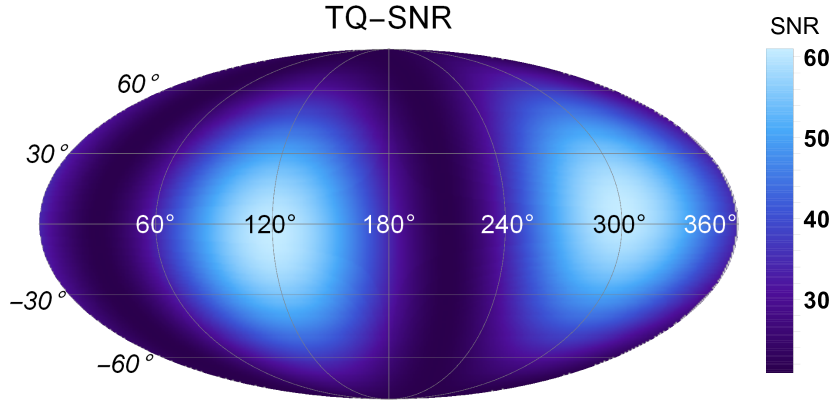
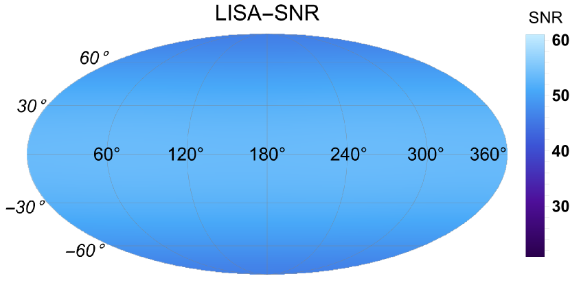
Figure 1: The distribution of SNR on the celestial sphere in ecliptic coordinate for TianQin and LISA.

In the following calculation, the position of the source will vary all over the celestial sphere, and the other parameters of the source are chosen as: $f=0.02\text{Hz},~{}\mathcal{A}=10^{-22},~{}\iota=\pi/4,~{}\psi_{s}=\pi/4$. The observation time is 1 year, and the results for $n$ years are just divided by $\sqrt{n}$ due to the monochromaticity of the source and the periodicity of the detector’s orbit. The SNR for the source at different position is given in Fig. 1, with upper panel for TianQin and bottom panel for LISA. We can see that for the chosen parameters, the SNR for the sources all over the sky is far beyond the threshold for detection, and thus satisfy the high SNR condition in FIM analysis.

TianQin will point to the DWD J0806 (the coordinate in ecliptic frame is $\theta_{s}=-4.7^{\circ}$ and $\phi_{s}=120.4^{\circ}$) and operate in the so-called “3+3” mode Luo et al. (2016), which means that the detector will follow the “three months on and three months off” working scheme, and thus the effective observation time ratio is $50\%$. So, we will also consider the twin constellation, which has another three crafts move along the orbit orthogonal to the primary TianQin constellation, so it will work during the primary constellation is off. We denote the two constellations as “TQ” and “TQ II”, respectively. The TianQin twin constellation will be denoted as “TQ I+II”. We will also calculate the capability of LISA and its joint detection with TianQin and the twin constellation.

III.1 Constraint on the Dipole Radiation

In this subsection, we will only consider the leading order dipole radiation of the extra modes.

For TianQin, the result is shown in Fig. 2. The result shows that the PE accuracy of $\alpha_{v}$ and $\alpha_{s}$ are strongly dependent on the location of the source. Especially, the result diverges for the direction of J0806 and its antipodal point. This feature is caused by the fact that the antenna pattern $F_{P}$ will be 0 for the sources at $\bar{\theta}=0,\pi$, and thus in the response signal, the components for the extra modes will be 0. However, for the other regions, the accuracy can be a few percent for vector and scalar mode, and the capability for vector mode is better than scalar mode.

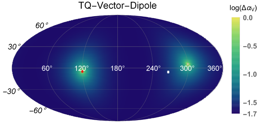
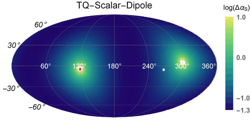
Figure 2: The distribution of $\Delta\alpha_{v}$ and $\Delta\alpha_{s}$ on the celestial sphere in ecliptic coordinate for TianQin. The red dot is J0806, and the white dot is the galactic center.

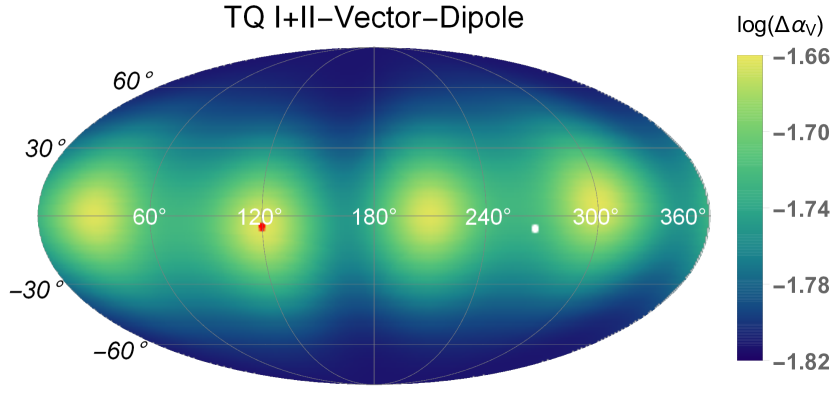
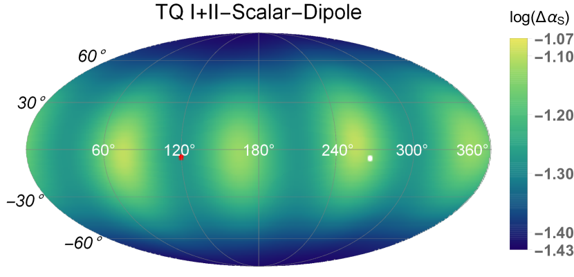
Figure 3: The distribution of $\Delta\alpha_{v}$ and $\Delta\alpha_{s}$ on the celestial sphere in ecliptic coordinate for the TianQin twin constellation.

The TianQin twin constellation is useful to avoid the divergent. Thus the results are a few percent for both extra modes all over the sky, as plotted in Fig. 3. However, we can see that the contour plot will be different for vector and scalar modes. For vector modes, the region near the orientations of the two constellations will be worse. But for scalar modes, the region between the orientations will be worse. This caused by the difference on the dependence of $\bar{\theta}$ for the response of the extra modes. For vector modes, as $\bar{\theta}$ approaches to 0, the response approaches to 0 as $\sin\bar{\theta}$. But the response for scalar modes will approaches to 0 as $\sin^{2}\bar{\theta}$. So although the result for both modes will divergent at $\bar{\theta}=0,\pi$, but the region near these points will be larger for scalar modes, since the response will grow slower as the sources move away from the divergent points.

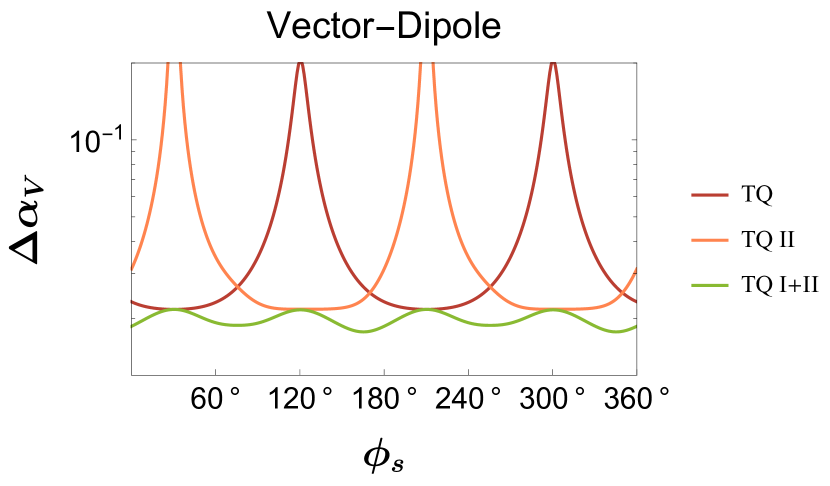
Figure 4: The distribution of $\Delta\alpha_{v}$ and $\Delta\alpha_{s}$ along the ecliptic plane for TQ (red line), TQ II (orange line) and TQ I+II (green line). Note that for TQ I+II, the better regions for the vector modes and the scalar modes located at different longitude.

In Fig. 4, we plot the accuracy of each mode for different detectors for the sources at the ecliptic plane. We should notice that the divergent point for TQ II located just on the ecliptic plane, and for TQ the result will be worst for the points has the same longitude as the divergent point. At the worst point for one detector, the accuracy will be the best for the other detector, and the result will be almost exact the value for the best one. But for the intermediate region between the divergent points, the accuracy will be almost the same for both detectors, and the joint detection will have an improvement for about $\sqrt{2}$ times. So for the vector modes, the PE result will decrease faster, and although the accuracy for the intermediate points will be worse than the best point for each detector, an improvement of $\sqrt{2}$ times will make it better than the best value. But for the scalar modes, the PE result will decrease slower, and an improvement of $\sqrt{2}$ times is still worse than the best value. Although the shape of the contours will be different, the results are still at the same order for the twin constellation all over the sky.

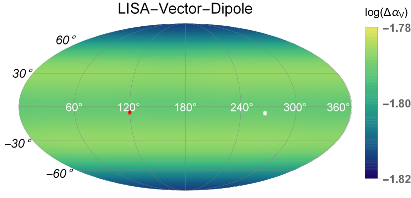
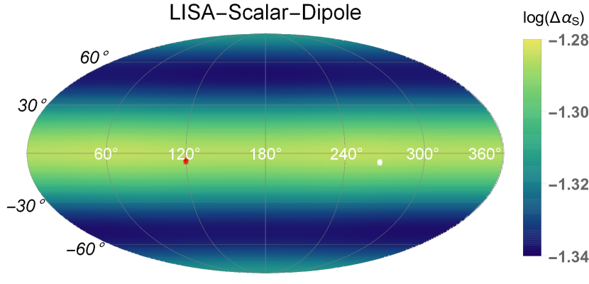
Figure 5: The distribution of $\Delta\alpha_{v}$ and $\Delta\alpha_{s}$ on the celestial sphere in ecliptic coordinate for LISA.

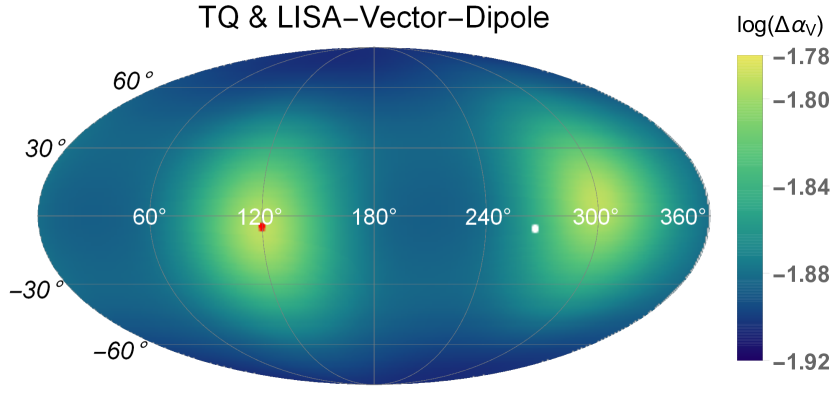
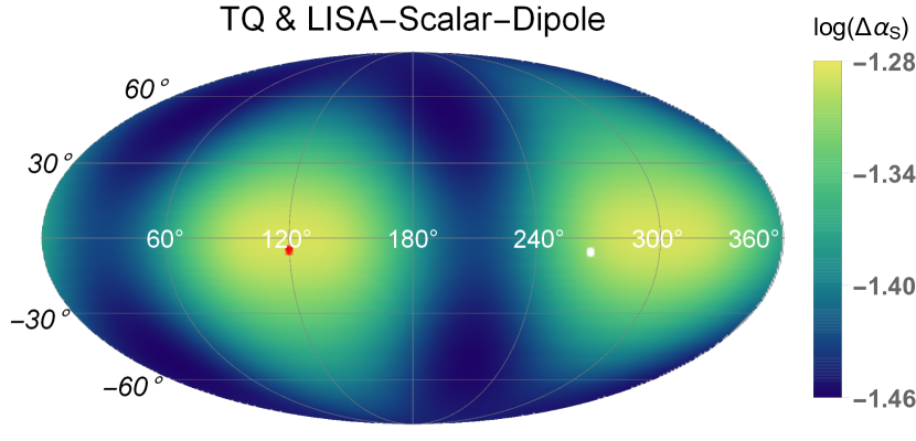
Figure 15: The distribution of $\Delta\alpha_{v}$ and $\Delta\alpha_{s}$ on the celestial sphere in ecliptic coordinate for the joint detection of TianQin and LISA.

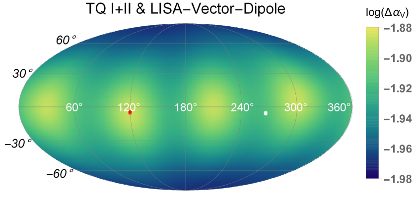
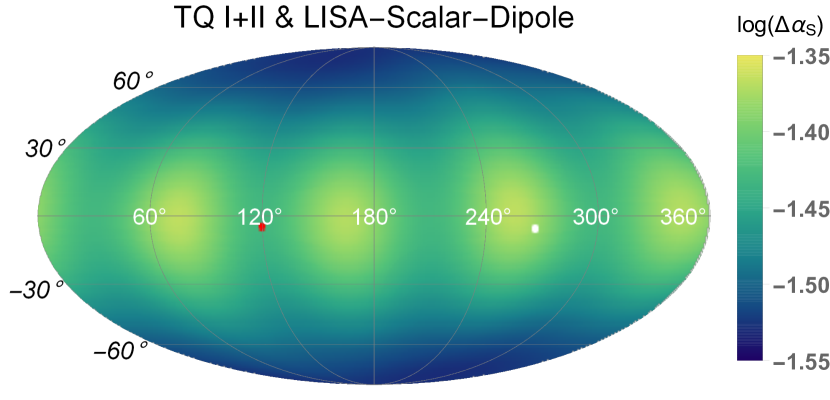
Figure 17: The distribution of $\Delta\alpha_{v}$ and $\Delta\alpha_{s}$ on the celestial sphere in ecliptic coordinate for the joint detection of TianQin twin constellation and LISA.

For LISA, as showed in Fig. 5, we can find that the accuracy is mainly determined by the latitude due to the periodic motion of LISA, and the result is about a few percent all over the sky. Additionally, we find that the distribution is different for vector and scalar modes. For the vector modes, the regions with better accuracy are located near the north and south pole. For the scalar modes, the accuracy will be worse for the region at the ecliptic plane and the poles. For the joint detection for LISA with TianQin or TianQin twin constellation, the accuracy will be improved, and the results are shown in Fig. 15 and Fig. 17 at Appendix A.

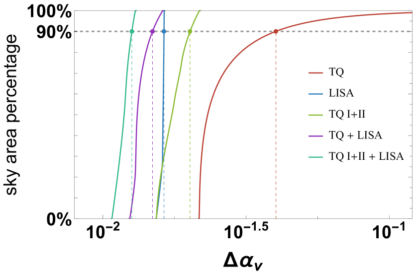
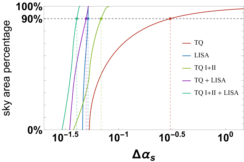
Figure 6: Top panel: the area ratio of sky region where the $\Delta\alpha_{v}$ always takes on a value less than a certain quantity. Bottom panel: same as the former one but for $\Delta\alpha_{s}$. The configurations considered include TQ, LISA, TQ I+II, TQ + LISA and TQ I+II + LISA. The dashed lines corresponding to the 90% threshold.

Table 1: The representative detecting accuracy for the 90% level and best of $\alpha_{v}$ and $\alpha_{s}$ for each configuration.

	TQ	TQ I+II	LISA	TQ + LISA	TQ I+II + LISA
$\Delta\alpha_{v}(90\%)$	0.040	0.020	0.016	0.015	0.013
$\Delta\alpha_{v}(\text{best})$	0.022	0.015	0.015	0.013	0.010
$\Delta\alpha_{s}(90\%)$	0.304	0.069	0.052	0.050	0.041
$\Delta\alpha_{s}(\text{best})$	0.054	0.040	0.048	0.036	0.030

For a more intuitive exhibition, we also plot the cumulative distribution function (CDF) of the accuracy distribution on the sky for each detector configuration in Fig. 6. The dashed line corresponds to the accuracy which can be achieved by 90% area in celestial sphere. The detailed results corresponding to this 90% threshold and the best accuracy for each configuration are shown in Table 1. From these figures, we can find that for TianQin, the distribution of the accuracy will have a very wide range due to the existence of the divergent point, although the best value can be comparable with other configurations. For all the other configurations, the distribution of the accuracy will be narrow, and Moreover, the accuracy for vector modes will be a few times better than the scalar modes in general.

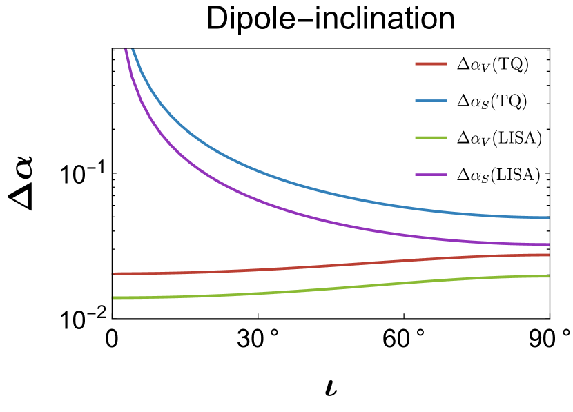
Figure 7: The distribution of $\Delta\alpha_{v}$ and $\Delta\alpha_{s}$ with different inclination angle for TianQin and LISA.

Despite the position of the source, the inclination angle will also have significant influence on the PE accuracy for the amplitude of extra polarizations. So here we consider the DWD source with different inclination angle, while the source position is chosen as $\theta_{s}=30^{\circ}$ and $\phi_{s}=60^{\circ}$. The dependence on inclination angle $\iota$ for $\Delta\alpha_{v}$ and $\Delta\alpha_{s}$ are shown in Fig. 7. If we choose another pair of position parameter, the result of $\Delta\alpha_{v}$ and $\Delta\alpha_{s}$ might have a moderate difference quantitatively, but the tendency of their dependence on $\iota$ will be similar. We find that $\Delta\alpha_{s}$ diverges when $\iota$ approaches to zero (face-on case) since the amplitude of scalar modes vanish for this case (cf. Eqs. (8) and (9)). Moreover, due to the different on the factor of $\iota$, the PE of the amplitude for extra modes will reach its best value at different $\iota$, which is $\pi/2$ for scalar modes, and $0$ for vector modes.

III.2 Constraint on the Quadrupole Radiation

For the sub-leading quadrupole radiation, the calculations are almost the same, except that we only consider these sub-leading term, and ignore the leading order dipole radiation.

The results for TianQin are shown in Fig. 8. We can find that the capability will be a few times worse than the dipole situation, and it will also have strong position dependence due to the vanish of the response. Due to the fact that the frequency of the extra modes at quadrupole order will be the same as the tensor mode, the degeneracy will happen between the angles and the relative amplitude of the extra modes. Thus except the divergent at the orientation of the detector, the result will also be worse on the plane of the detector for scalar modes, and on the direction perpendicular to the orientation and located on the ecliptic plane. The second additional degeneracy is caused by the degeneracy between $\alpha^{\prime}_{v}$ and $\theta_{s}$. As we plotted in Fig. 9, if we exclude the parameter $\theta_{s}$, then the region on the ecliptic plane and perpendicular to the orientation will disappear.

Figure 8: The distribution of $\Delta\alpha^{\prime}_{v}$ and $\Delta\alpha^{\prime}_{s}$ on the celestial sphere in ecliptic coordinate for TianQin.

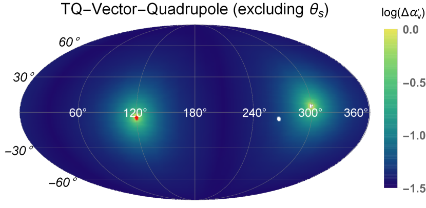
Figure 9: The distribution of $\Delta\alpha^{\prime}_{v}$ on the celestial sphere for TianQin, with $\theta_{s}$ excluded in the PE.

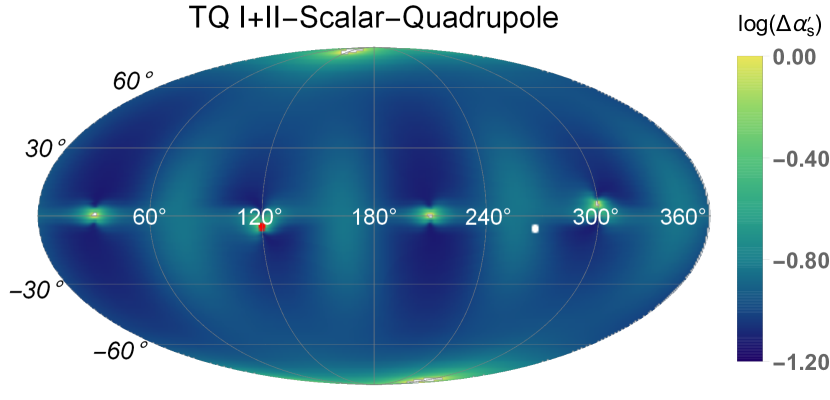
Figure 10: The distribution of $\Delta\alpha^{\prime}_{v}$ and $\Delta\alpha^{\prime}_{s}$ on the celestial sphere in ecliptic coordinate for the TianQin twin constellation.

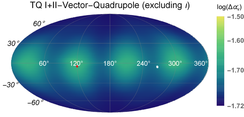
Figure 11: The distribution of $\Delta\alpha^{\prime}_{v}$ on the celestial sphere for TianQin twin constellation, with $\iota$ excluded in the PE.

The results for the TianQin twin constellation are displayed in Fig. 10. The position dependence will also be deduced as for the dipole case, but the shape will be different for the vector mode. This is caused by the degeneracy between $\alpha^{\prime}_{v}$ and $\iota$. After removing the inclination angle $\iota$ in the FIM analysis, we can find that the result looks like the plot for dipole case (see upper panel of Fig. 3). As a comparison, we show it in Fig. 11. The detailed shape is caused by the choice of the value for $\iota$, and it will also change if we change $\iota$.

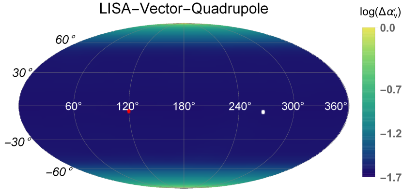
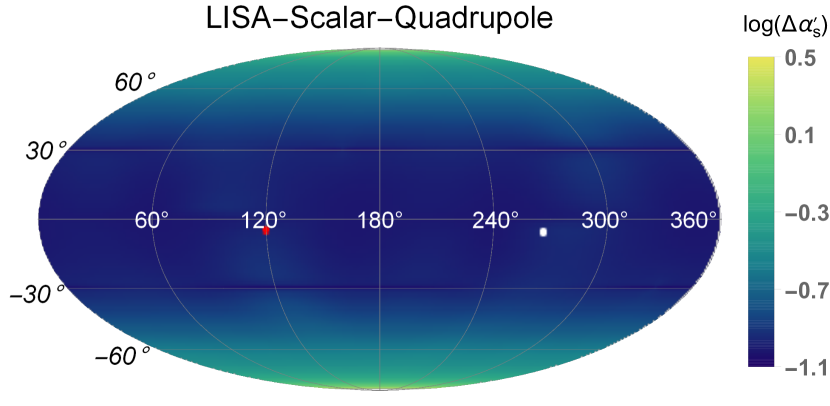
Figure 12: The distribution of $\Delta\alpha^{\prime}_{v}$ and $\Delta\alpha^{\prime}_{s}$ on the celestial sphere in ecliptic coordinate for LISA.

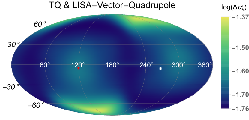
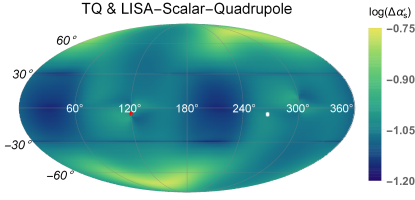
Figure 16: The distribution of $\Delta\alpha^{\prime}_{v}$ and $\Delta\alpha^{\prime}_{s}$ on the celestial sphere in ecliptic coordinate for the joint detection of TianQin and LISA.

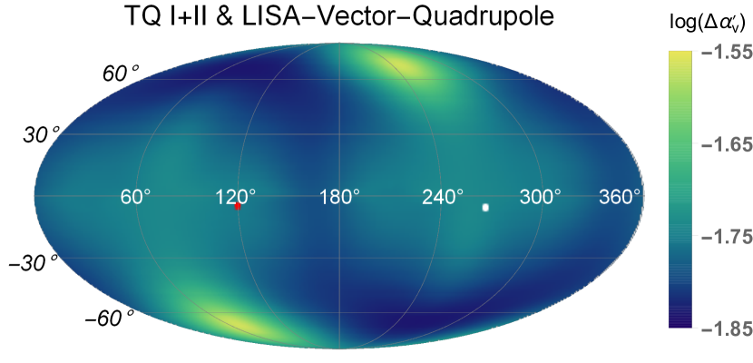
Figure 18: The distribution of $\Delta\alpha^{\prime}_{v}$ and $\Delta\alpha^{\prime}_{s}$ on the celestial sphere in ecliptic coordinate for the joint detection of TianQin twin constellation and LISA.

For LISA, we can find that the detecting accuracy is mainly determined by the latitude of the source location, same as the dipole case. But this time, the worse part will be the pole region for both vector and scalar modes. The result is shown in Fig. 12. For the joint detection for LISA with TianQin or TianQin twin constellation, the accuracy will also be improved, and the results are shown in Fig. 16 and Fig. 18 at Appendix A.

Again, we plot the CDF of the accuracy distribution on the sky for each detector configuration in Fig. 13, and list the result for the best value and $90\%$ threshold in Table 2. Except for TianQin, LISA will also have a very wide distribution due to the degeneracy between the relative amplitude and the angles. But the result for joint detection will still be narrow due to the complementary of different detectors. Overall, the accuracy for dipole radiation will be a few times better than that for the quadrupole radiation. Since the amplitude of the leading dipole radiation would also be stronger than the sub-leading quadrepole radiation, this result means that it will be better to constrain the extra modes with dipole radiation, if we ignore the problem of identification of the common origin.

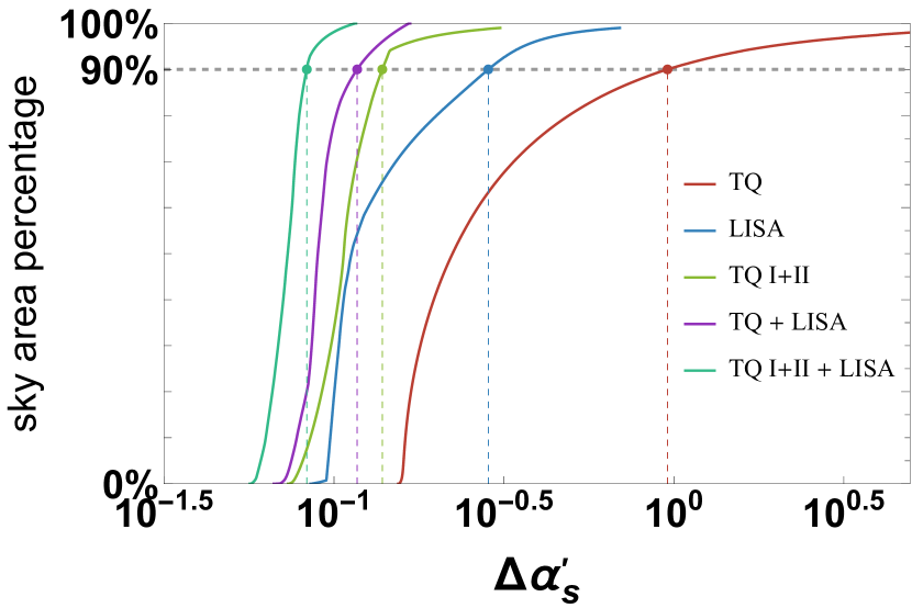
Figure 13: Upper panel: the area ratio of sky region where the $\Delta\alpha^{\prime}_{v}$ always takes on a value less than a certain quantity. Bottom panel: same as the former one but for $\Delta\alpha^{\prime}_{s}$. The configurations considered include TQ, LISA, TQ I+II, TQ + LISA and TQ I+II + LISA. The dashed lines corresponding to the 90% threshold.

Table 2: The representative detecting accuracy for the 90% level and best of $\alpha^{\prime}_{v}$ and $\alpha^{\prime}_{s}$ for each configuration.

	TQ	TQ I+II	LISA	TQ + LISA	TQ I+II + LISA
$\Delta\alpha^{\prime}_{v}(90\%)$	0.076	0.030	0.049	0.024	0.019
$\Delta\alpha^{\prime}_{v}(\text{best})$	0.034	0.019	0.023	0.018	0.014
$\Delta\alpha^{\prime}_{s}(90\%)$	0.958	0.139	0.284	0.117	0.083
$\Delta\alpha^{\prime}_{s}(\text{best})$	0.156	0.073	0.088	0.069	0.056

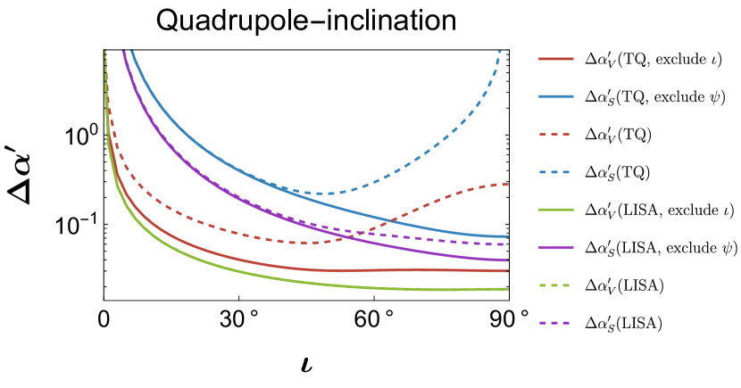
Figure 14: The distribution of $\Delta\alpha^{\prime}_{v}$ and $\Delta\alpha^{\prime}_{s}$ with different inclination angle for TianQin and LISA.

Same as the dipole case, the PE accuracy for the sub-leading quadrupole radiation will also be sensitive to inclination angle of the source. Here we also consider the DWD source with different inclination angle by fixing the source position to $\theta_{s}=30^{\circ}$ and $\phi_{s}=60^{\circ}$. The dependence on inclination angle $\iota$ for $\Delta\alpha^{\prime}_{v}$ and $\Delta\alpha^{\prime}_{s}$ are shown in Fig. 14. We find that both $\Delta\alpha^{\prime}_{v}$ and $\Delta\alpha^{\prime}_{s}$ diverge when $\iota$ becomes zero since all the extra modes both vanish for the face-on DWD (cf. Eqs. (10-13)). Moreover, we can see that only for the TianQin consternation, $\iota\to\pi/2$ can bring the degeneracy between some angle parameters and the extra mode amplitudes (especially $\iota$ and $\alpha^{\prime}_{v}$, $\psi$ and $\alpha^{\prime}_{s}$). When we exclude $\iota$ and $\psi$ respectively in the PE, the degeneracy disappears and $\Delta\alpha^{\prime}_{v,s}$ has the smallest value at $\iota=\pi/2$.

IV Constraint with verification binaries

As mentioned in Huang et al. (2020), despite the thousands of DWDs which could be detected in the future observation, we can also detect several VBs which have already been detected by EM observations. For VBs, the position and frequency of the VBs can be determined by EM observation, and the accuracy of the position is much better than the GW observations, which means that we don’t need to consider the PE of the two position angles in the FIM analysis. However, since the accuracy of frequency with EM observation is worse than the GW observation, the frequency will still be considered in the FIM analysis. Thus the parameters will be reduced to only six while $\theta_{s}$ and $\phi_{s}$ will be known parameters. As we mentioned above, there will be degeneracy between the relative amplitudes and the positions of the source, so if the position is determined through the EM observation, the constraint of the extra modes will be better. Moreover, for part of VBs, their inclination angle could also be determined by EM observations such as intensity interferometry Baumgartner et al. (2020) with better precision comparing to the GW observation. Thus the parameter $\iota$ can be excluded in the FIM analysis. The parameters of the VBs are listed in Table 3. For another part of VBs there is no direct measurement on the inclination angle through EM observation and the angle is assigned based on other information of the binary system Huang et al. (2020). We label the estimated values of $\iota$ with the asterisk. Note that we must consider the PE of the inclination angle for these special VBs in FIM analysis.

Table 3: The parameters of VBs which can be detected by TianQin within 5 years. The asterisk after the values means the parameter has no precise EM measurement.

source	$\theta$	$\phi$	$\iota$	$f$/mHz	$\mathcal{A}$
J0806	94.7	120.4	38	6.22	$1.28\times 10^{-22}$
ZTF J1539	23.8	205.0	84	4.82	$3.68\times 10^{-22}$
V407 Vul	43.2	295.0	60∗	3.51	$2.20\times 10^{-22}$
ES Cet	110.3	24.6	60∗	3.22	$2.14\times 10^{-22}$
SDSS J0651	94.2	101.3	87	2.61	$3.24\times 10^{-22}$
SDSS J1351	85.5	208.4	60∗	2.12	$1.24\times 10^{-22}$
AM CVn	52.6	170.4	43	1.94	$5.66\times 10^{-22}$
SDSS J1908	28.5	298.2	15	1.84	$1.22\times 10^{-22}$
HP Lib	85.0	235.1	30∗	1.81	$3.14\times 10^{-22}$
SDSS J0935	61.9	131.0	60∗	1.68	$5.98\times 10^{-22}$
SDSS J2322	81.5	353.4	27	1.66	$1.74\times 10^{-22}$
PTF J0533	111.1	82.9	73	1.62	$1.52\times 10^{-22}$
CR Boo	72.1	202.3	30∗	1.36	$2.58\times 10^{-22}$
V803 Cen	120.3	216.2	14	1.25	$3.20\times 10^{-22}$

Here we will consider TQ, LISA, TQ I+II, TQ + LISA and TQ I+II + LISA. The mission lifetime is 4 yrs for LISA, and 5 yrs for TianQin with 4 years overlap with LISA.The results are shown in Table 4 for dipole case, and in Table 5 for quadrupole case. The results of J0806 in the first two column are invalid since the estimated errors diverge in the sky location of J0806 for TQ due to the zero response of the extra modes. However, due to the suitable frequency and the strong amplitude, the capability for other configurations can still reach to a few percent or less. In Tables 4 and 5, for J0806, ZTF J1539, SDSS J0651, AM CVn, SDSS J1908, SDSS J2322, PTF J0533 and V803 Cen, the FIMs are calculated with fixed $\iota$.

Table 4: The PE accuracy of dipole amplitude $\alpha_{v}$ and $\alpha_{s}$ for the VBs.

	TQ		LISA		TQ I+II		TQ + LISA		TQ I+II + LISA
	$\Delta\alpha_{v}$	$\Delta\alpha_{s}$	$\Delta\alpha_{v}$	$\Delta\alpha_{s}$	$\Delta\alpha_{v}$	$\Delta\alpha_{s}$	$\Delta\alpha_{v}$	$\Delta\alpha_{s}$	$\Delta\alpha_{v}$	$\Delta\alpha_{s}$
J0806	\	\	0.008	0.031	0.035	0.103	0.008	0.031	0.008	0.029
ZTF J1539	0.026	0.037	0.005	0.009	0.018	0.028	0.005	0.009	0.005	0.008
V407 Vul	0.090	0.305	0.022	0.046	0.056	0.123	0.021	0.046	0.020	0.043
ES Cet	0.089	0.164	0.030	0.068	0.080	0.162	0.029	0.063	0.028	0.063
SDSS J0651	0.225	1.342	0.041	0.077	0.093	0.159	0.041	0.076	0.038	0.069
SDSS J1351	0.360	0.658	0.158	0.377	0.358	0.658	0.145	0.327	0.145	0.327
AM CVn	0.090	0.285	0.038	0.113	0.063	0.217	0.035	0.105	0.032	0.100
SDSS J1908	0.433	4.538	0.167	1.526	0.286	2.477	0.155	1.445	0.144	1.299
HP Lib	0.173	0.784	0.072	0.350	0.150	0.767	0.066	0.318	0.064	0.317
SDSS J0935	0.172	0.712	0.051	0.113	0.097	0.214	0.049	0.111	0.045	0.100
SDSS J2322	0.400	2.485	0.149	0.804	0.291	2.007	0.138	0.760	0.132	0.746
PTF J0533	0.686	2.065	0.230	0.439	0.445	1.070	0.218	0.429	0.204	0.406
CR Boo	0.362	1.363	0.142	0.664	0.327	1.353	0.132	0.597	0.130	0.596
V803 Cen	0.326	2.787	0.124	1.252	0.270	2.709	0.116	1.142	0.113	1.136

Table 5: The PE accuracy of quadrupole amplitude $\alpha^{\prime}_{v}$ and $\alpha^{\prime}_{s}$ for the VBs.

	TQ		LISA		TQ I+II		TQ + LISA		TQ I+II + LISA
	$\Delta\alpha^{\prime}_{v}$	$\Delta\alpha^{\prime}_{s}$	$\Delta\alpha^{\prime}_{v}$	$\Delta\alpha^{\prime}_{s}$	$\Delta\alpha^{\prime}_{v}$	$\Delta\alpha^{\prime}_{s}$	$\Delta\alpha^{\prime}_{v}$	$\Delta\alpha^{\prime}_{s}$	$\Delta\alpha^{\prime}_{v}$	$\Delta\alpha^{\prime}_{s}$
J0806	\	\	0.010	0.049	0.018	0.054	0.010	0.044	0.009	0.036
ZTF J1539	0.007	0.651	0.003	0.010	0.006	0.043	0.003	0.009	0.003	0.009
V407 Vul	0.035	0.141	0.006	0.016	0.019	0.053	0.006	0.016	0.006	0.015
ES Cet	0.029	0.453	0.006	0.018	0.024	0.054	0.006	0.018	0.006	0.017
SDSS J0651	0.056	3.114	0.005	0.017	0.025	0.049	0.005	0.016	0.005	0.016
SDSS J1351	0.114	4.142	0.024	0.076	0.102	0.201	0.023	0.073	0.023	0.071
AM CVn	0.033	0.172	0.008	0.030	0.023	0.123	0.008	0.029	0.008	0.029
SDSS J1908	0.395	6.216	0.107	1.293	0.290	4.088	0.104	1.277	0.100	1.218
HP Lib	0.115	0.635	0.023	0.145	0.099	0.482	0.022	0.140	0.022	0.137
SDSS J0935	0.065	0.317	0.011	0.031	0.028	0.078	0.011	0.030	0.010	0.029
SDSS J2322	0.206	1.878	0.061	0.421	0.158	1.503	0.059	0.411	0.057	0.404
PTF J0533	0.230	1.132	0.047	0.127	0.220	0.792	0.046	0.125	0.044	0.123
CR Boo	0.236	3.229	0.071	0.415	0.164	0.735	0.066	0.377	0.065	0.360
V803 Cen	0.342	31.95	0.146	1.802	0.286	3.360	0.135	1.633	0.130	1.584

We can find that, among all the VBs, ZTF J1539 can constrain the amplitude $\alpha_{v}$ and $\alpha_{s}$ to 0.005 and 0.008 respectively with TQ I+II + LISA, which is the best result. That is the combined effect of the higher amplitude of ZTF J1539 with suitable frequency, and the advantage sky location which at the best region as plotted in the previous figures. However, the accuracy of quadrupole mode constrained with TianQin will be worse for ZTF J1539, and the reason is that its position located near the detector’s plane of TianQin, and we plotted in the bottom panel in Fig. 8, those sources will have strong degeneracy with angular parameters.

V Conclusion and Discussion

We investigated the capability of TianQin to probe the extra polarizations in GWs. We considered not only the standard TianQin constellation , but also the twin constellations and their joint detection with LISA. We construct the responded signal with all the six polarizations, and assume that the GW waveform is monochromatic for DWDs. Fisher analysis is adopted to estimate the accuracy to measure the parameters. We defined two parameters, $\alpha_{v}$ and $\alpha_{s}$, to describe the dipole amplitudes of the extra modes relative to the tensor modes, and $\alpha^{\prime}_{v}$ and $\alpha^{\prime}_{s}$ for quadrupole amplitudes. Doppler effect due to the periodical motion of the detector around the Sun is also considered in the signal construction.

We first analyze the behaviour of the PE accuracy for the relative amplitudes as the function of the source position, and listed the best accuracy and the accuracy which can be attained by more than 90% sky zone to describe the overall capability in the polarization detection. We find that, for TQ, the PE accuracy will divergent at the orientation due to the zero response, and thus have very strong dependency on the sky location of the source, ranging across about 2 orders. However, the capability of TianQin can still reach to a few percent for most of the regions. The application of the twin constellation can significantly improve this strong position dependent feature. A joint detection with LISA will also improve the result for a few times.

Generally, for all the detector configurations and both dipole and quadrupole situations, the capability for vector modes will be better than that for scalar modes. On the other hand, the capability for dipole radiation will also be better than that for quadrupole radiation. For the quadrupole case, the amplitude of the extra modes will have strong degeneracy with the position and the direction of the angular momentum. However, due to the difficulty in the identification of the common origin, it’s still very useful to consider the quadrupole radiation.

Finally, we also considered the capabilities with the observation of the VBs. For most of the VBs, the capabilities are about a few percents. However, due to the zero response of the extra modes, TianQin could not detect the extra modes with J0806, although its expected to be one of the most loudest DWDs. We also find that, for the best source ZTF J1539, the capability will be even less than one percent.

However, our analysis only focus on the monochromatic DWD signals. But the space borne GW detectors can also detect many other chirping sources, such as binary black holes or EMRIs. Some modelling works for these sources which focused on the extra polarization modes have already been done in recent years for some specific gravitational theories. But for a more general analysis, we still need a parametric model. In the future, we will consider the non-monochromatic sources and including the propagation effect and the modification of the phase.

Appendix A Results for the joint detection

To reduce the length of the main text, we plot the results for the joint detection of TianQin and LISA in this appendix. The analysis of these results is presented in Sec. III, and we will not repeat it here.

References

- Abbott et al. (2016a) B. Abbott et al. (LIGO Scientific Collaboration and Virgo Collaboration), Phys. Rev. Lett. 116, 061102 (2016a), arXiv:1602.03837 [gr-qc] .
- Abbott et al. (2016b) B. P. Abbott et al. (LIGO Scientific, Virgo), Phys. Rev. X 6, 041015 (2016b), arXiv:1606.04856 [gr-qc] .
- Abbott et al. (2019a) B. P. Abbott et al. (LIGO Scientific, Virgo), Phys. Rev. X 9, 031040 (2019a), arXiv:1811.12907 [astro-ph.HE] .
- Abbott et al. (2021a) R. Abbott et al. (LIGO Scientific, Virgo), Phys. Rev. X 11, 021053 (2021a), arXiv:2010.14527 [gr-qc] .
- Abbott et al. (2021b) R. Abbott et al. (LIGO Scientific, VIRGO), (2021b), arXiv:2108.01045 [gr-qc] .
- Abbott et al. (2021c) R. Abbott et al. (LIGO Scientific, VIRGO, KAGRA), (2021c), arXiv:2111.03606 [gr-qc] .
- Abbott et al. (2016c) B. P. Abbott et al. (LIGO Scientific, Virgo), Phys. Rev. Lett. 116, 221101 (2016c), [Erratum: Phys.Rev.Lett. 121, 129902 (2018)], arXiv:1602.03841 [gr-qc] .
- Abbott et al. (2019b) B. Abbott et al. (LIGO Scientific, Virgo), Phys. Rev. Lett. 123, 011102 (2019b), arXiv:1811.00364 [gr-qc] .
- Abbott et al. (2019c) B. Abbott et al. (LIGO Scientific, Virgo), Phys. Rev. D 100, 104036 (2019c), arXiv:1903.04467 [gr-qc] .
- Abbott et al. (2021d) R. Abbott et al. (LIGO Scientific, Virgo), Phys. Rev. D 103, 122002 (2021d), arXiv:2010.14529 [gr-qc] .
- Abbott et al. (2021e) R. Abbott et al. (LIGO Scientific, VIRGO, KAGRA), (2021e), arXiv:2112.06861 [gr-qc] .
- Punturo et al. (2010) M. Punturo et al., Class. Quant. Grav. 27, 194002 (2010).
- Abbott et al. (2017a) B. P. Abbott et al. (LIGO Scientific), Class. Quant. Grav. 34, 044001 (2017a), arXiv:1607.08697 [astro-ph.IM] .
- Luo et al. (2016) J. Luo et al. (TianQin), Class. Quant. Grav. 33, 035010 (2016), arXiv:1512.02076 [astro-ph.IM] .
- Amaro-Seoane et al. (2017) P. Amaro-Seoane et al. (LISA), “Laser Interferometer Space Antenna,” (2017), arXiv:1702.00786 [astro-ph.IM] .
- Eardley et al. (1973a) D. Eardley, D. Lee, A. Lightman, R. Wagoner, and C. Will, Phys. Rev. Lett. 30, 884 (1973a).
- Eardley et al. (1973b) D. Eardley, D. Lee, and A. Lightman, Phys. Rev. D 8, 3308 (1973b).
- Gong and Hou (2018a) Y. Gong and S. Hou, Universe 4, 85 (2018a), arXiv:1806.04027 [gr-qc] .
- Will (2014) C. M. Will, Living Rev. Rel. 17, 4 (2014), arXiv:1403.7377 [gr-qc] .
- Maggiore and Nicolis (2000) M. Maggiore and A. Nicolis, Phys. Rev. D 62, 024004 (2000), arXiv:gr-qc/9907055 .
- Capozziello and Corda (2006) S. Capozziello and C. Corda, Int. J. Mod. Phys. D 15, 1119 (2006).
- Rizwana Kausar et al. (2016) H. Rizwana Kausar, L. Philippoz, and P. Jetzer, Phys. Rev. D 93, 124071 (2016), arXiv:1606.07000 [gr-qc] .
- Gong and Hou (2018b) Y. Gong and S. Hou, EPJ Web Conf. 168, 01003 (2018b), arXiv:1709.03313 [gr-qc] .
- Katsuragawa et al. (2019) T. Katsuragawa, T. Nakamura, T. Ikeda, and S. Capozziello, Phys. Rev. D 99, 124050 (2019), arXiv:1902.02494 [gr-qc] .
- Moretti et al. (2019) F. Moretti, F. Bombacigno, and G. Montani, Phys. Rev. D 100, 084014 (2019), arXiv:1906.01899 [gr-qc] .
- Gong et al. (2018) Y. Gong, S. Hou, D. Liang, and E. Papantonopoulos, Phys. Rev. D 97, 084040 (2018), arXiv:1801.03382 [gr-qc] .
- Sagi (2010) E. Sagi, Phys. Rev. D 81, 064031 (2010), arXiv:1001.1555 [gr-qc] .
- de Paula et al. (2004) W. L. de Paula, O. D. Miranda, and R. M. Marinho, Class. Quant. Grav. 21, 4595 (2004), arXiv:gr-qc/0409041 .
- Abbott et al. (2017b) B. Abbott et al. (LIGO Scientific, Virgo), Phys. Rev. Lett. 119, 141101 (2017b), arXiv:1709.09660 [gr-qc] .
- Guersel and Tinto (1989) Y. Guersel and M. Tinto, Phys. Rev. D 40, 3884 (1989).
- Wen and Schutz (2005) L. Wen and B. F. Schutz, Class. Quant. Grav. 22, S1321 (2005), arXiv:gr-qc/0508042 .
- Wen (2008) L. Wen, Int. J. Mod. Phys. D 17, 1095 (2008), arXiv:gr-qc/0702096 .
- Chatterji et al. (2006) S. Chatterji, A. Lazzarini, L. Stein, P. J. Sutton, A. Searle, and M. Tinto, Phys. Rev. D 74, 082005 (2006), arXiv:gr-qc/0605002 .
- Hagihara et al. (2018) Y. Hagihara, N. Era, D. Iikawa, and H. Asada, Phys. Rev. D 98, 064035 (2018), arXiv:1807.07234 [gr-qc] .
- Hagihara et al. (2019) Y. Hagihara, N. Era, D. Iikawa, A. Nishizawa, and H. Asada, Phys. Rev. D 100, 064010 (2019), arXiv:1904.02300 [gr-qc] .
- Hagihara et al. (2020) Y. Hagihara, N. Era, D. Iikawa, N. Takeda, and H. Asada, Phys. Rev. D 101, 041501 (2020), arXiv:1912.06340 [gr-qc] .
- Pang et al. (2020) P. T. Pang, R. K. Lo, I. C. Wong, T. G. Li, and C. Van Den Broeck, Phys. Rev. D 101, 104055 (2020), arXiv:2003.07375 [gr-qc] .
- Wong et al. (2021) I. C. F. Wong, P. T. H. Pang, R. K. L. Lo, T. G. F. Li, and C. V. D. Broeck, “Null-stream-based bayesian unmodeled framework to probe generic gravitational-wave polarizations,” (2021), arXiv:2105.09485 [gr-qc] .
- Takeda et al. (2022) H. Takeda, S. Morisaki, and A. Nishizawa, Phys. Rev. D 105, 084019 (2022), arXiv:2105.00253 [gr-qc] .
- Chatziioannou et al. (2012) K. Chatziioannou, N. Yunes, and N. Cornish, Phys. Rev. D 86, 022004 (2012), [Erratum: Phys.Rev.D 95, 129901 (2017)], arXiv:1204.2585 [gr-qc] .
- Takeda et al. (2018) H. Takeda, A. Nishizawa, Y. Michimura, K. Nagano, K. Komori, M. Ando, and K. Hayama, Phys. Rev. D 98, 022008 (2018), arXiv:1806.02182 [gr-qc] .
- Isi et al. (2015) M. Isi, A. J. Weinstein, C. Mead, and M. Pitkin, Phys. Rev. D 91, 082002 (2015), arXiv:1502.00333 [gr-qc] .
- Isi et al. (2017) M. Isi, M. Pitkin, and A. J. Weinstein, Phys. Rev. D 96, 042001 (2017), arXiv:1703.07530 [gr-qc] .
- Abbott et al. (2018) B. P. Abbott et al. (LIGO Scientific, Virgo), Phys. Rev. Lett. 120, 031104 (2018), arXiv:1709.09203 [gr-qc] .
- Isi et al. (2020) M. Isi, S. Mastrogiovanni, M. Pitkin, and O. J. Piccinni, Phys. Rev. D 102, 123027 (2020), arXiv:2010.12612 [gr-qc] .
- da Silva Alves and Tinto (2011) M. E. da Silva Alves and M. Tinto, Phys. Rev. D 83, 123529 (2011), arXiv:1102.4824 [gr-qc] .
- Lee et al. (2008) K. J. Lee, F. A. Jenet, and R. H. Price, The Astrophysical Journal 685, 1304 (2008).
- Niu and Zhao (2019) R. Niu and W. Zhao, Sci. China Phys. Mech. Astron. 62, 970411 (2019), arXiv:1812.00208 [gr-qc] .
- O’Beirne et al. (2019) L. O’Beirne, N. J. Cornish, S. J. Vigeland, and S. R. Taylor, Phys. Rev. D 99, 124039 (2019), arXiv:1904.02744 [gr-qc] .
- Boîtier et al. (2020) A. Boîtier, S. Tiwari, L. Philippoz, and P. Jetzer, Phys. Rev. D 102, 064051 (2020), arXiv:2008.13520 [gr-qc] .
- Arzoumanian et al. (2020) Z. Arzoumanian et al. (NANOGrav), Astrophys. J. Lett. 905, L34 (2020), arXiv:2009.04496 [astro-ph.HE] .
- Chen et al. (2021) Z.-C. Chen, C. Yuan, and Q.-G. Huang, Sci. China Phys. Mech. Astron. 64, 120412 (2021), arXiv:2101.06869 [astro-ph.CO] .
- Arzoumanian et al. (2021) Z. Arzoumanian et al. (NANOGrav), Astrophys. J. Lett. 923, L22 (2021), arXiv:2109.14706 [gr-qc] .
- Klein et al. (2016) A. Klein et al., Phys. Rev. D 93, 024003 (2016), arXiv:1511.05581 [gr-qc] .
- Feng et al. (2019) W.-F. Feng, H.-T. Wang, X.-C. Hu, Y.-M. Hu, and Y. Wang, Phys. Rev. D 99, 123002 (2019), arXiv:1901.02159 [astro-ph.IM] .
- Wang et al. (2019) H.-T. Wang et al., Phys. Rev. D 100, 043003 (2019), arXiv:1902.04423 [astro-ph.HE] .
- Babak et al. (2017) S. Babak, J. Gair, A. Sesana, E. Barausse, C. F. Sopuerta, C. P. Berry, E. Berti, P. Amaro-Seoane, A. Petiteau, and A. Klein, Phys. Rev. D 95, 103012 (2017), arXiv:1703.09722 [gr-qc] .
- Fan et al. (2020) H.-M. Fan, Y.-M. Hu, E. Barausse, A. Sesana, J.-d. Zhang, X. Zhang, T.-G. Zi, and J. Mei, Phys. Rev. D 102, 063016 (2020), arXiv:2005.08212 [astro-ph.HE] .
- Robson et al. (2018) T. Robson, N. J. Cornish, N. Tamanini, and S. Toonen, Phys. Rev. D 98, 064012 (2018), arXiv:1806.00500 [gr-qc] .
- Lau et al. (2020) M. Y. Lau, I. Mandel, A. Vigna-Gómez, C. J. Neijssel, S. Stevenson, and A. Sesana, Mon. Not. Roy. Astron. Soc. 492, 3061 (2020), arXiv:1910.12422 [astro-ph.HE] .
- Liu et al. (2020) S. Liu, Y.-M. Hu, J.-d. Zhang, and J. Mei, Phys. Rev. D 101, 103027 (2020), arXiv:2004.14242 [astro-ph.HE] .
- Huang et al. (2020) S.-J. Huang, Y.-M. Hu, V. Korol, P.-C. Li, Z.-C. Liang, Y. Lu, H.-T. Wang, S. Yu, and J. Mei, Phys. Rev. D 102, 063021 (2020), arXiv:2005.07889 [astro-ph.HE] .
- Romano and Cornish (2017) J. D. Romano and N. J. Cornish, Living Rev. Rel. 20, 2 (2017), arXiv:1608.06889 [gr-qc] .
- Liang et al. (2022) Z.-C. Liang, Y.-M. Hu, Y. Jiang, J. Cheng, J.-d. Zhang, and J. Mei, Phys. Rev. D 105, 022001 (2022), arXiv:2107.08643 [astro-ph.CO] .
- Burdge et al. (2019) K. B. Burdge et al., Nature 571, 528 (2019), arXiv:1907.11291 [astro-ph.SR] .
- Will (1994) C. M. Will, Phys. Rev. D 50, 6058 (1994), arXiv:gr-qc/9406022 .
- Sennett et al. (2016) N. Sennett, S. Marsat, and A. Buonanno, Phys. Rev. D 94, 084003 (2016), arXiv:1607.01420 [gr-qc] .
- Poisson and Will (2014) E. Poisson and C. M. Will, Gravity: Newtonian, post-newtonian, relativistic (Cambridge University Press, 2014).
- Roelofs et al. (2010) G. H. A. Roelofs, A. Rau, T. R. Marsh, D. Steeghs, P. J. Groot, and G. Nelemans, Astrophys. J. Lett. 711, L138 (2010), arXiv:1003.0658 [astro-ph.SR] .
- Peters and Mathews (1963) P. C. Peters and J. Mathews, Phys. Rev. 131, 435 (1963).
- Nelemans et al. (2001) G. Nelemans, L. R. Yungelson, and S. F. Portegies Zwart, Astron. Astrophys. 375, 890 (2001), arXiv:astro-ph/0105221 .
- Zhang et al. (2019) C. Zhang, Q. Gao, Y. Gong, D. Liang, A. J. Weinstein, and C. Zhang, Phys. Rev. D 100, 064033 (2019), arXiv:1906.10901 [gr-qc] .
- Hu et al. (2018) X.-C. Hu, X.-H. Li, Y. Wang, W.-F. Feng, M.-Y. Zhou, Y.-M. Hu, S.-C. Hu, J.-W. Mei, and C.-G. Shao, Class. Quant. Grav. 35, 095008 (2018), arXiv:1803.03368 [gr-qc] .
- Zhang et al. (2020) C. Zhang, Q. Gao, Y. Gong, B. Wang, A. J. Weinstein, and C. Zhang, Phys. Rev. D 101, 124027 (2020), arXiv:2003.01441 [gr-qc] .
- Rubbo et al. (2004) L. J. Rubbo, N. J. Cornish, and O. Poujade, Phys. Rev. D 69, 082003 (2004), arXiv:gr-qc/0311069 .
- Vallisneri (2008) M. Vallisneri, Phys. Rev. D 77, 042001 (2008), arXiv:gr-qc/0703086 .
- Finn (1992) L. S. Finn, Phys. Rev. D 46, 5236 (1992), arXiv:gr-qc/9209010 .
- Cutler and Flanagan (1994) C. Cutler and E. E. Flanagan, Phys. Rev. D 49, 2658 (1994), arXiv:gr-qc/9402014 .
- Robson et al. (2019) T. Robson, N. J. Cornish, and C. Liu, Class. Quant. Grav. 36, 105011 (2019), arXiv:1803.01944 [astro-ph.HE] .
- Baumgartner et al. (2020) S. Baumgartner, M. Bernardini, J. R. Canivete Cuissa, H. de Laroussilhe, A. M. W. Mitchell, B. A. Neuenschwander, P. Saha, T. Schaeffer, D. Soyuer, and L. Zwick, Mon. Not. Roy. Astron. Soc. 498, 4577 (2020), arXiv:2008.11538 [astro-ph.IM] .