Parameterization-Independent Importance Sampling of Environment Maps

Abstract

Environment maps with high dynamic range lighting, such as daylight sky maps, require importance sampling to keep the balance between noise and number of samples per pixel manageable. Typically, importance sampling schemes for environment maps are based directly on the map parameterization, e.g. equirectangular maps, and do not work with alternative parameterizations that might provide better sampling quality. In this paper, an importance sampling scheme based on an equal-area projection of the sphere is proposed that is easy to implement and works independently of the environment map parameterization or resolution. This allows to apply the same scheme to equirectangular maps, cube map variants, or any other map representation, and to adapt the importance sampling granularity to the requirements of the map contents.

I Introduction

In physically based rendering, high dynamic range environment maps can provide realistic lighting of scenes. In such maps, the lighting is often distributed very unevenly. For example, in daylight sky maps, the small region that represents the sun is thousands of times brighter than other regions of the sky. Importance sampling is therefore required to keep noise in the rendering result at acceptable levels while limiting the required number of samples per pixel.

The importance sampling scheme for environment maps is typically based directly on the environment map parameterization. For example, the Mitsuba and pbrt renderers support environment maps using the equirectangular (latitude-longitude) parameterization and build auxiliary maps in the same parameterization to create light direction samples and compute corresponding probability density function values [1]. However, equirectangular maps are known to suffer from strong distortions especially in the polar areas, which reduces sampling quality. Other parameterizations of environment maps, such as classical cube maps [2] or low-distortion variants thereof [3] provide better sampling quality, but supporting them requires tailored importance sampling schemes.

We propose to decouple the importance sampling scheme from the environment map parameterization and its resolution. Our importance sampling scheme is based on an equal-area projection between sphere and square, which simplifies the required computations. It can be applied to all environment map parameterizations and allows adapting its granularity to reduce computational costs.

II Related Work

This paper focusses on importance sampling and multiple importance sampling for Monte Carlo renderers, not on alternative techniques like product importance sampling [4, 5] or optimizations for special cases [6], methods that focus on visibility considerations [7, 8], or methods for dynamic environment maps [9].

Importance sampling strategies for environment maps in Monte Carlo renderers typically compute importance maps based on the environment map parameterization, and use them as the base to generate light direction samples and to compute the underlying probability density function. For example, both the Mitsuba and pbrt renderers support equirectangular environment maps and precompute equirectangular importance maps to enable importance sampling [1]. Agarwal et al. apply hierarchical structuring to equirectangular maps [10], and Lu et al. base importance maps on the cube map representation used in their real-time renderer [11].

In these cases, supporting different types of environment map parameterizations is difficult since they require derivation of tailored importance sampling schemes. This paper therefore proposes to decouple the importance sampling from the environment map parameterization.

III Method

A basic environment map implementation in a renderer typically only needs one function $L(\vec{d})$ to return a radiance spectrum or RGB sample for a lookup direction $\vec{d}$.

To support importance sampling, an implementation additionally needs to a way to generate light direction samples according to a suitable probability density function. To support multiple importance sampling, this functionality is separated into a function $p(\vec{d})$ that computes the probability density function value for a given direction and a function $d()$ that generates a random light direction sample according to $p$.

Traditionally, these functions all work on the same environment map parameterization. In our approach, the sampling function $L(\vec{d})$ still uses the original environment map representation to make sure that sampling quality remains the same, while functions $p(\vec{d})$ and $d()$ work on importance maps that are tailored to their needs. This means that these functions only need to be implemented once and will work with any environment map parameterization. A minimal C++ interface that implements this approach is shown in Fig. 1.

⬇

class EnvMap {

// Functions implemented in subclasses such as

// EnvMapEquirect, EnvMapCube:

// Sample the environment map.

virtual Spectrum L(vec3 d);

// Functions implemented only once, independent

// of subclasses:

// Return the pdf value for direction d:

float p(vec3 d);

// Generate a random direction according to p:

vec3 d();

};

Figure 1: Minimal interface of an environment map that supports multiple importance sampling.

For good importance sampling results, the value of the probability density function $p$ for a direction $\vec{d}$ must be proportional to a suitable importance measure $I(\vec{d})$ for that direction: $p(\vec{d})\propto I(\vec{d})$. Here the sum of radiances over the spectrum is used as the importance measure: $I(\vec{d})=\sum_{i=1}^{k}L(\vec{d})$ for a spectrum with $k$ samples ($k=3$ for RGB environment maps). Note that other measures can be used, e.g. a luminance value computed from the spectrum as used by Mitsuba and pbrt.

Furthermore, to be a valid probability distribution function, $p$ must integrate to 1 over the surface of the unit sphere: $\int_{S^{2}}pd\omega=1$.

Our implementation of the functions $d()$ and $p(\vec{d})$ is based on an importance map $M$, a sorted importance map $M_{s}$, and a cumulative sorted importance map $M_{cs}$. These maps are based on an equal-area projection between sphere and square described in Sec. III-A. Their construction is described in Sec. III-B. Values of the probability density function $p(\vec{d})$ can be taken directly from map $M$, as described in Sec. III-C, and light direction samples for function $d()$ can be generated based on maps $M_{cs}$ and $M_{s}$, as described in Sec. III-D.

III-A Equal Area Projection between sphere and square

Using an equal area projection between sphere and square to generate the importance maps has the advantage that uniformly distributed random numbers on the 2D square translate directly to uniformly generated random numbers on the unit sphere surface, which simplifies both the sampling of light directions and the evaluation of the probability density function.

The unit sphere surface is first projected to the unit disk using the Lambert Azimuthal Equal-Area projection [12] and the unit disk is then projected to the unit square using Shirley’s equal area projection [13].

The resulting mapping function $m:S^{2}\rightarrow[0,1]^{2}$ first maps a direction $\vec{d}$ represented as latitude $\theta$ and longitude $\varphi$ to a point on the unit disk represented as radius $r$ and angle $\alpha$, and then to a point $(u,v)$ in the unit square:
$r=\sin\left(\frac{\frac{\pi}{2}-\theta}{2}\right)\quad\alpha=\varphi-\frac{\pi}{2}\quad\alpha^{\prime}=\begin{cases}\alpha&\alpha\geq-\frac{\pi}{4}\\ \alpha+2\pi&\alpha<-\frac{\pi}{4}\end{cases}$
$(u^{\prime},v^{\prime})=\begin{cases}(r,\frac{\alpha^{\prime}r}{\frac{\pi}{4}})&\alpha^{\prime}<\frac{\pi}{4}\\ (-(\alpha^{\prime}-\frac{\pi}{2})\frac{r}{\frac{\pi}{4}},r)&\alpha^{\prime}<\frac{3\pi}{4}\\ (-r,(\alpha^{\prime}-\pi)\frac{-r}{\frac{\pi}{4}})&\alpha^{\prime}<\frac{5\pi}{4}\\ (-(\alpha^{\prime}-\frac{3\pi}{2})\frac{-r}{\frac{\pi}{4}},-r)&\text{otherwise}\\ \end{cases}$
$u=\frac{1}{2}(u^{\prime}+1)\quad v=\frac{1}{2}(v^{\prime}+1)$

The inverse mapping is defined as follows:
$u^{\prime}=2u-1\quad v^{\prime}=2v-1$
$(r,\alpha)=\begin{cases}(u^{\prime},\frac{\pi}{4}\frac{v^{\prime}}{u^{\prime}})&u^{\prime 2}>v^{\prime 2}\\ (v^{\prime},\frac{\pi}{2}-\frac{\pi}{4}\frac{u^{\prime}}{v^{\prime}})&u^{\prime 2}\leq v^{\prime 2}\\ (0,0)&u^{\prime}=v^{\prime}=0\\ \end{cases}$
$\theta=\frac{\pi}{2}-2\sin^{-1}(r)\quad\varphi=\alpha+\frac{\pi}{2}$

Note that this equal-area map is only used to generate light directions and to look up probability density function values. The sampling of the environment still takes place in the original environment map parameterization. This means that we benefit from the equal-area property of the map, which results in significant simplifications, but are unaffected by its distortions and discontinuities [14].

The map projection is demonstrated in Fig. 2 using the Earth’s land masses as an illustration for the mapping from sphere to square. For the inverse mapping, the square map is divided into a raster of $32\times 32$ colored squares and reprojected onto a sphere. Angular distortions and discontinuities are visible, but all reprojected areas are of the same size.

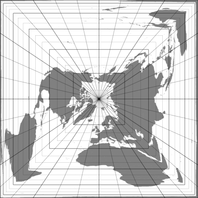
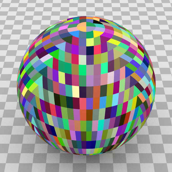
Figure 2: The equal area square map of the sphere. Left: the Earth’s land masses on the square map; the south pole is mapped to the border. Right: a colored raster on the square map reprojected onto the sphere.

III-B Importance Maps

Three maps of size $N\times N$ are precomputed using the map projection defined in Sec. III-A as a base for the importance sampling scheme:

1. The importance map $M$ which in each bin $(i,j)$ stores the importance measure for the corresponding direction $\vec{d}$, normalized so that the sum over all $N\times N$ bins is 1. First, importance values $M[i][j]=I\left(m^{-1}\left(\frac{i+\frac{1}{2}}{N},\frac{j+\frac{1}{2}}{N}\right)\right)$ are computed and from them the total importance sum $I_{\text{total}}=\sum_{i=1}^{N}\sum_{j=1}^{N}M[i][j]$. Afterwards, each bin value is divided by $I_{\text{total}}$.

2. The sorted importance map $M_{s}$ which stores bin indices so that $M[M_{s}[i][j]]$ is sorted according to descending normalized importance. In practice, $M_{s}$ can simply store 1D integer indices $\{0,\ldots,N^{2}-1\}$.

3. The cumulative sorted importance map $M_{cs}$ which stores cumulative normalized importances according to $M_{s}$ so that $M_{cs}[0][0]=\max_{i,j}M[i][j]$ and $M_{cs}[N-1][N-1]=\sum_{i=1}^{N}\sum_{j=1}^{N}M[i][j]=1$.

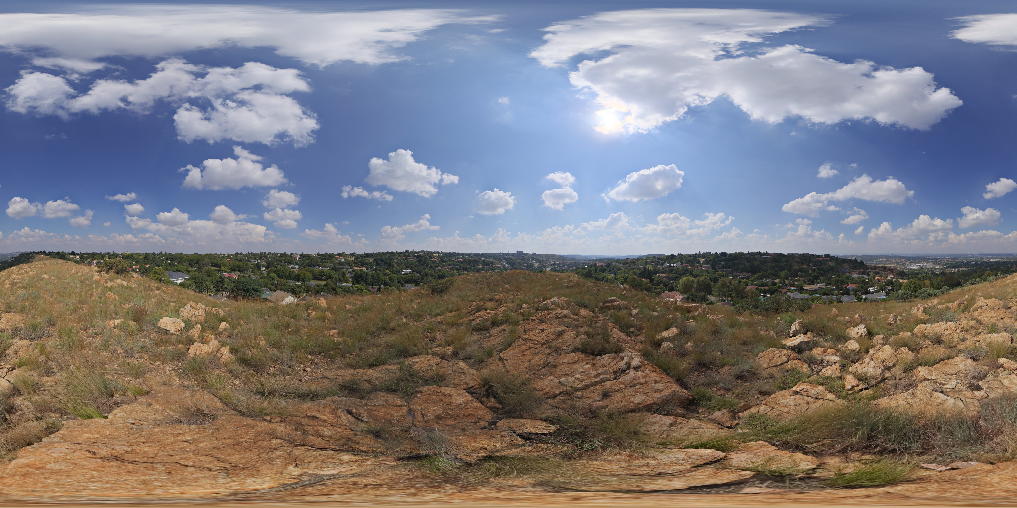
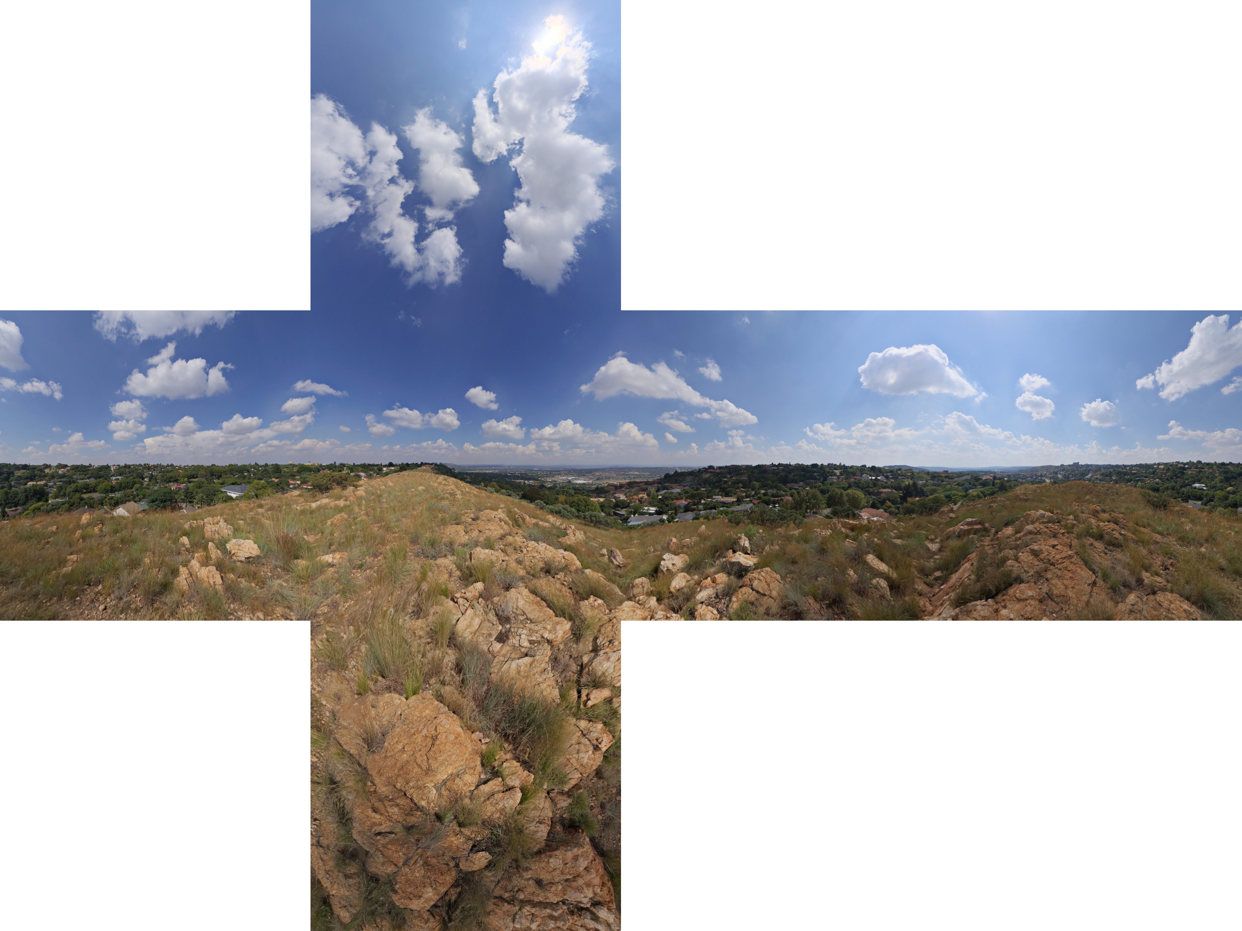
Figure 3: A daylight sky environment map in equirectangular (left) and cube map (right) parameterization.

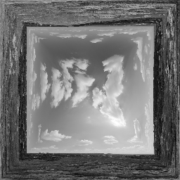
Figure 4: The importance maps $M$ (left) and $M_{s}$ (right) computed from the environment map shown in Fig. 3.

The map size $N\times N$ is independent of the resolution of the environment map. This approach assumes approximately constant importance of all directions covered by one bin reprojected onto the sphere. Therefore, $N$ should be chosen so that the dominant light sources in the environment map can be sampled with enough precision, i.e. the bin size is small enough to provide a reasonable representation of them. Only extreme cases of very bright light sources covering only a few pixels in the environment map parameterization require to chose $N$ so that the total number of importance map entries is roughly equal to the resolution of the original environment map; in most cases, $N$ can be chosen significantly lower to save memory and computation time.

Fig. 3 shows a daylight sky environment map in equirectangular and cube map parameterizations. Fig. 4 shows the maps $M$ and $M_{s}$ computed from either of those parameterizations for $N=256$.

III-C Probability density function

By construction, the entries in map $M$ represent the importance of the corresponding directions in the environment map. To compute a probability density function value from them, the normalized map entries need to be divided by the size $s$ of one bin on the unit sphere: $s=\frac{4\pi}{N^{2}}$. This enforces the requirement that $\int_{S^{2}}pd\omega=1$.

To get the probability density function value for a given direction $\vec{d}$, map coordinates $(u,v)=m(\vec{d})$ are translated into a bin index $(i,j)$:
$(u,v)=m(\vec{d})\quad(i,j)=(\lfloor Nu\rfloor,\lfloor Nv\rfloor)\quad p(\vec{d})=\frac{M[i][j]}{s}$

III-D Sampling light directions

To generate light direction samples with the probability density function $p$ described in Sec. III-C, maps $M_{cs}$ and $M_{s}$ are used as follows:

• Generate a uniformly distributed random number $r\in[0,1)$

• Find the entry $(i^{\prime},j^{\prime})$ with the cumulative normalized importance $r$ in the map $M_{cs}$. Binary search can be applied for this purpose.

• Get the corresponding bin index in map $M$ from $M_{s}$: $(i,j)=M_{s}[i^{\prime}][j^{\prime}]$.

• Based on uniformly distributed random numbers $s_{0},s_{1}\in[0,1)$, create map coordinates $(u,v)$ inside the bin $(i,j)$:
  $u=\frac{i+s_{0}}{N}\quad v=\frac{j+s_{1}}{N}$

• The direction sample is $\vec{d}=m^{-1}(u,v)$.

Uniform sampling inside a bin works because the importance map projection is equal area, otherwise the samples would not correspond to uniformly distributed samples on the unit sphere surface patch represented by the bin.

Fig. 5 shows 5000 light direction samples produced with this method overlaid over the two parameterizations of the original environment map.

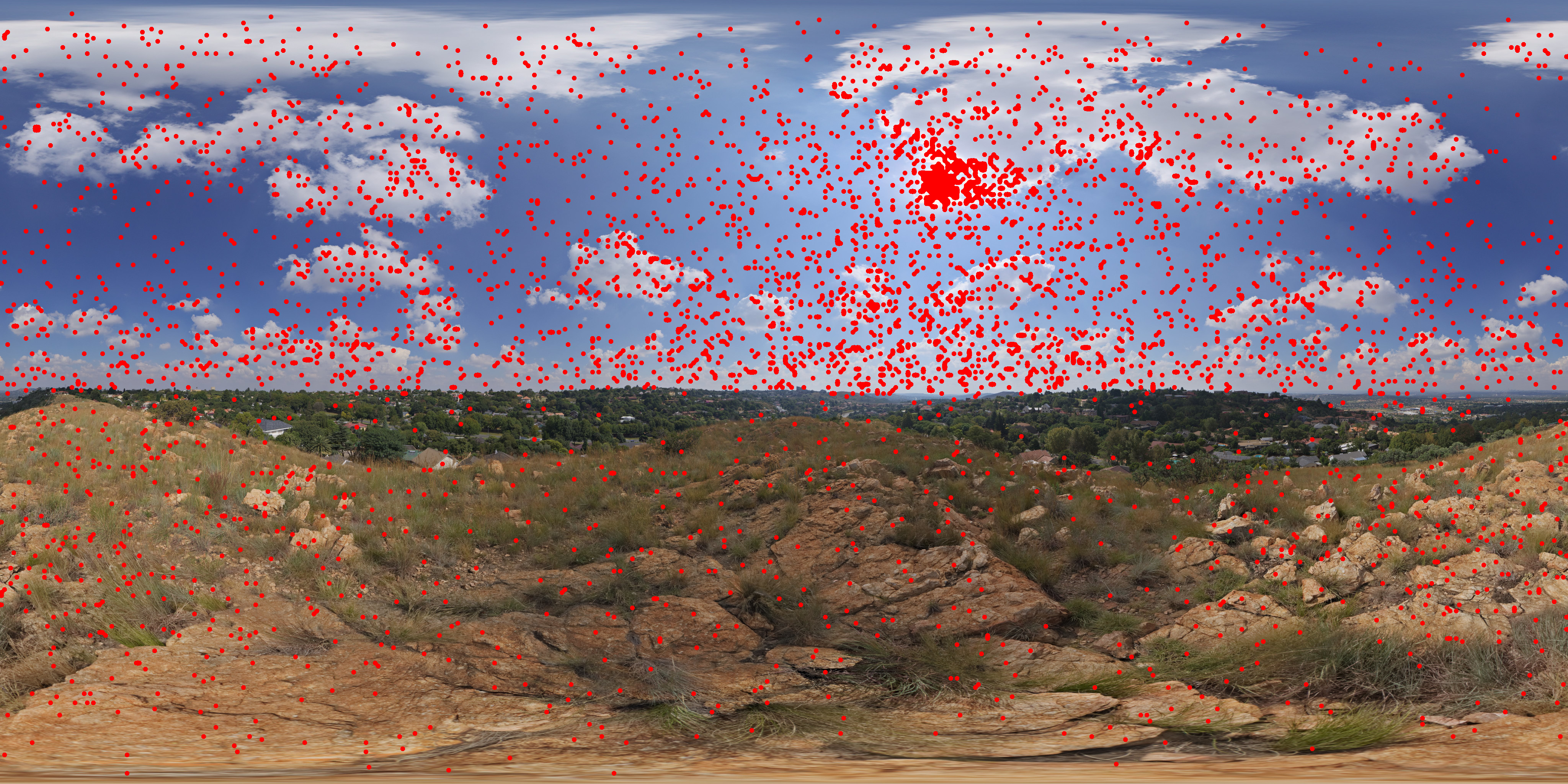
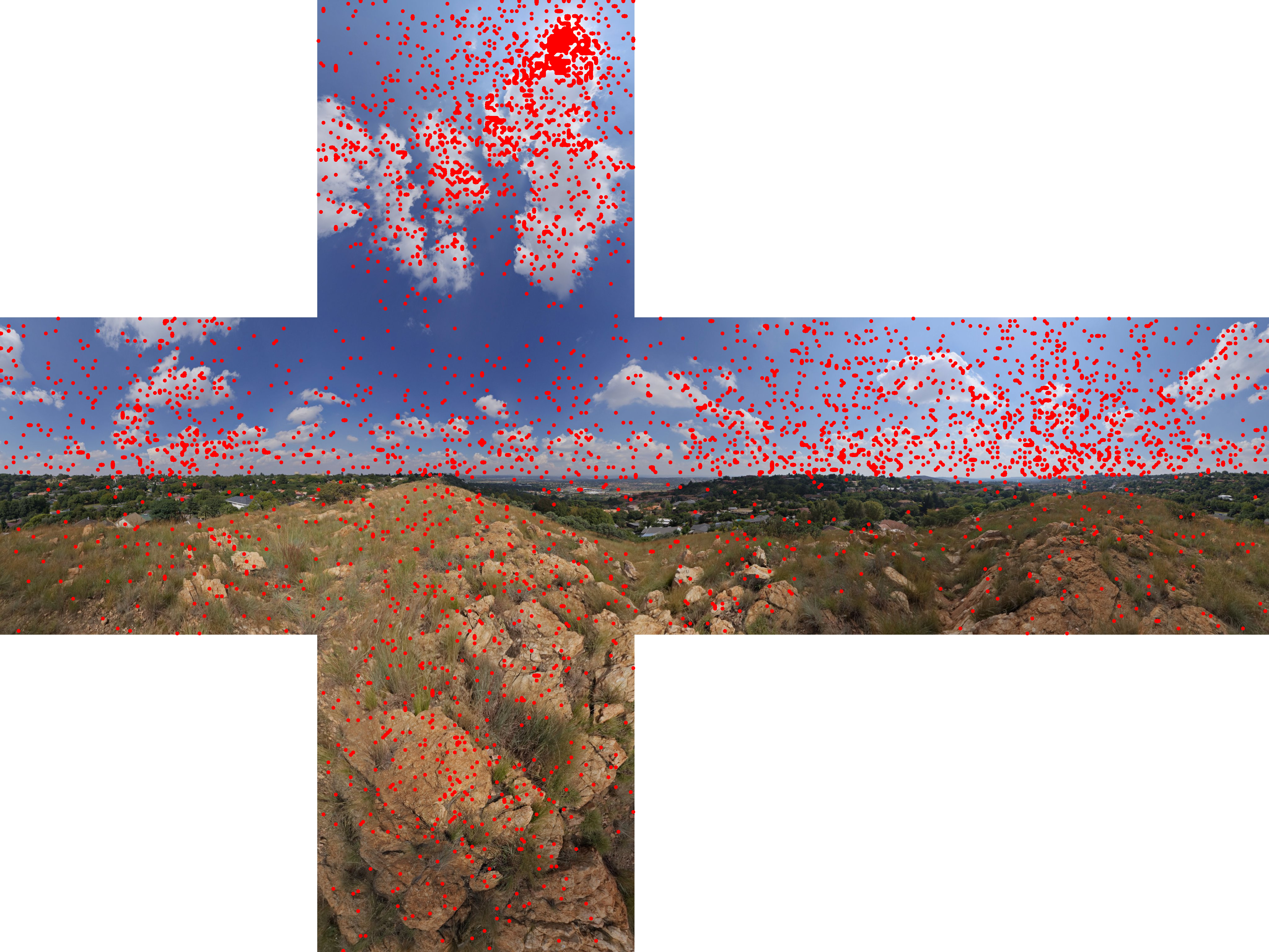
Figure 5: 5000 light direction samples taken with the method described in Sec. III-D overlaid over the equirectangular (left) and cube (right) environment map parameterizations.

IV Results

We implemented our importance sampling scheme as part of a Monte Carlo path tracer with support for multiple importance sampling.

Fig. 6 shows an example scene rendered at 64 samples per pixel without and with environment map importance sampling. The importance map size parameter $N$ was doubled in each step. For values of $N$ greater than 1024, no quality improvements were visible, which suggests that the underlying equirectangular environment map of size $4096\times 2048$ is adequately represented by an importance map of size $1024\times 1024$. Note that both Mitsuba and pbrt build importance map structures at the equirectangular image resolution instead. The mirroring sphere on the left demonstrates that the resolution of the environment map parameterization remains the same regardless of parameter $N$.

Rendering the same scene but with a cube environment map parameterization with a resolution of $1024\times 1024$ per cube side does not result in noticeable differences, as expected.

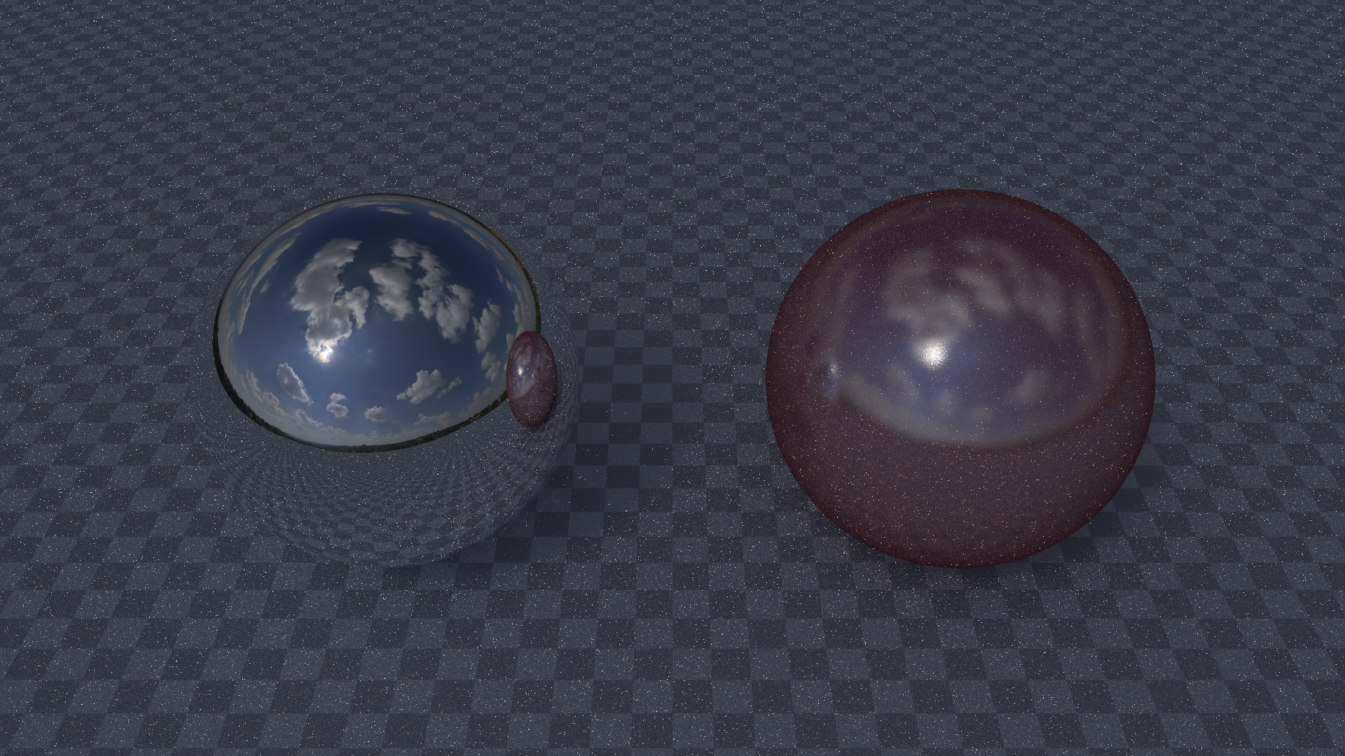
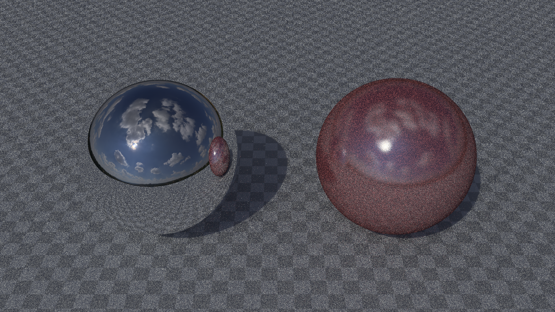
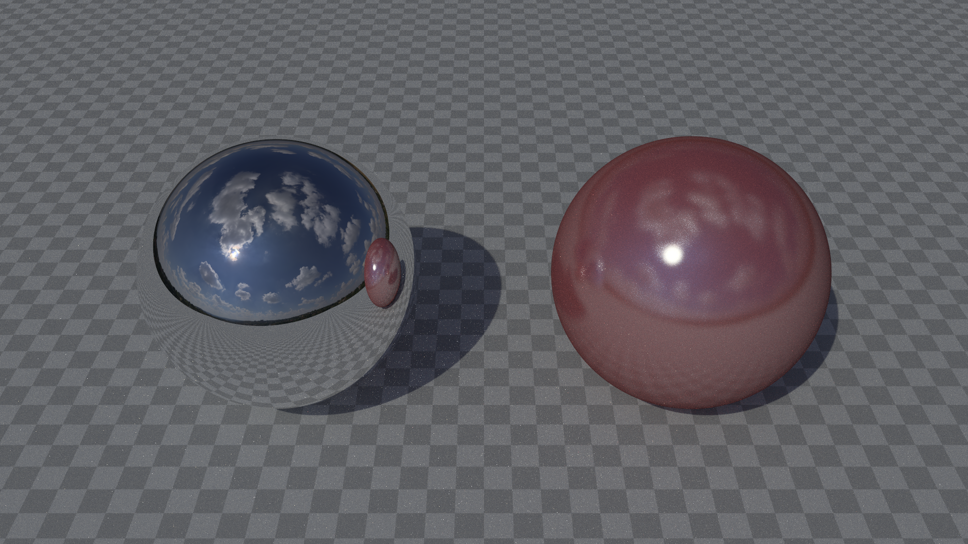
Figure 6: A scene rendered at 64 samples per pixel without (top) and with environment map importance sampling with parameter $N=256$ (middle) and $N=1024$ (bottom).

Modifying the scene by making the right sphere perfectly diffuse enabled reproducing scene and parameters as closely as possible for the Mitsuba renderer. For 64 samples per pixel and $N=1024$, there were no visible quality differences to Mitsuba’s result, confirming that higher resolution importance map structures are not necessary for this typical example of a daylight sky map.

Fig. 7 shows results for environment maps with more evenly distributed lighting: a cloudy sky map and an indoor map, both given as equirectangular maps of size $4096\times 2048$. For such maps, $N$ can be chosen significantly lower without loss of quality: $N=64$ for the cloudy sky and $N=128$ for the indoor map. This results in significant reduction of memory consumption.

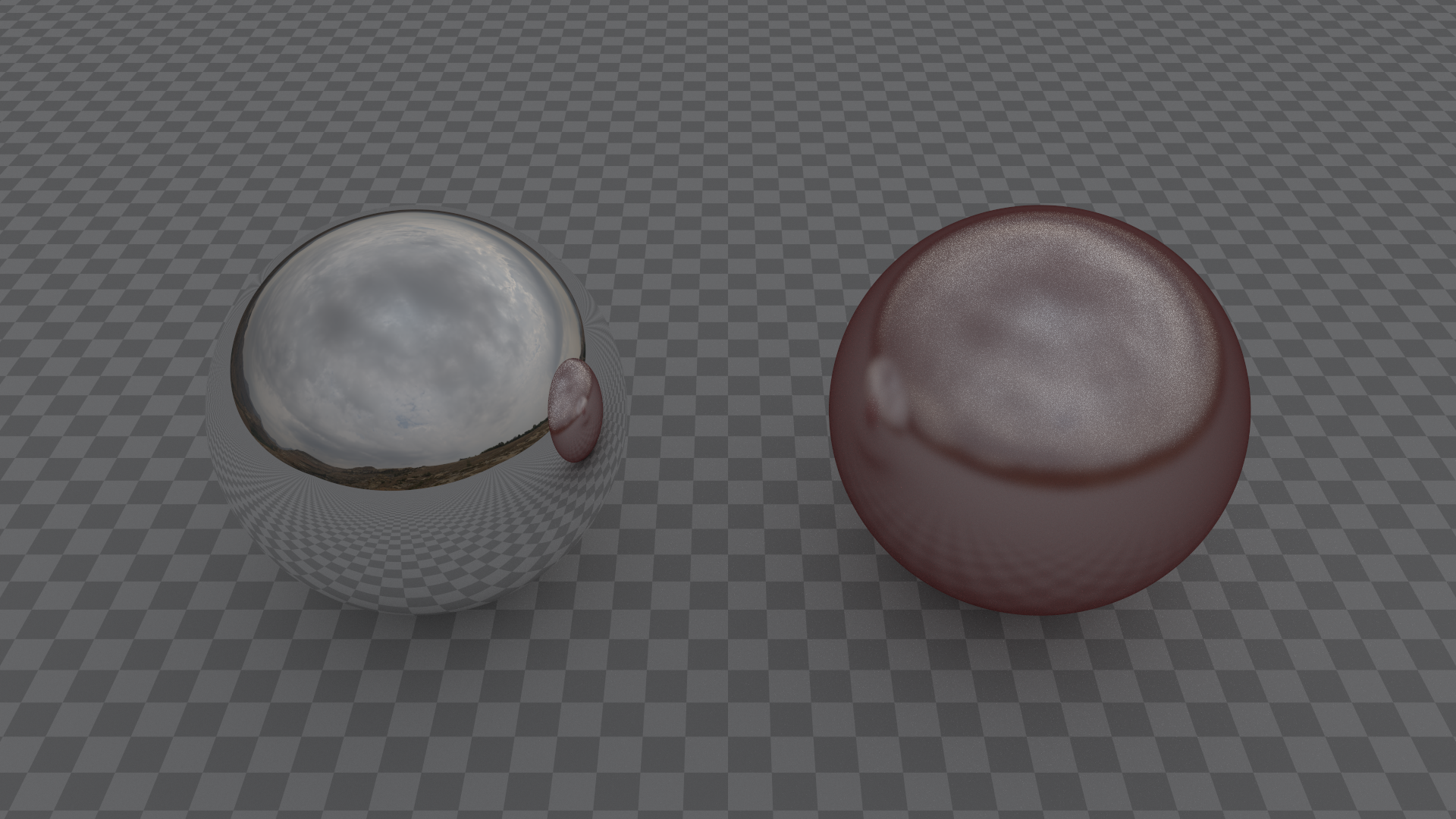
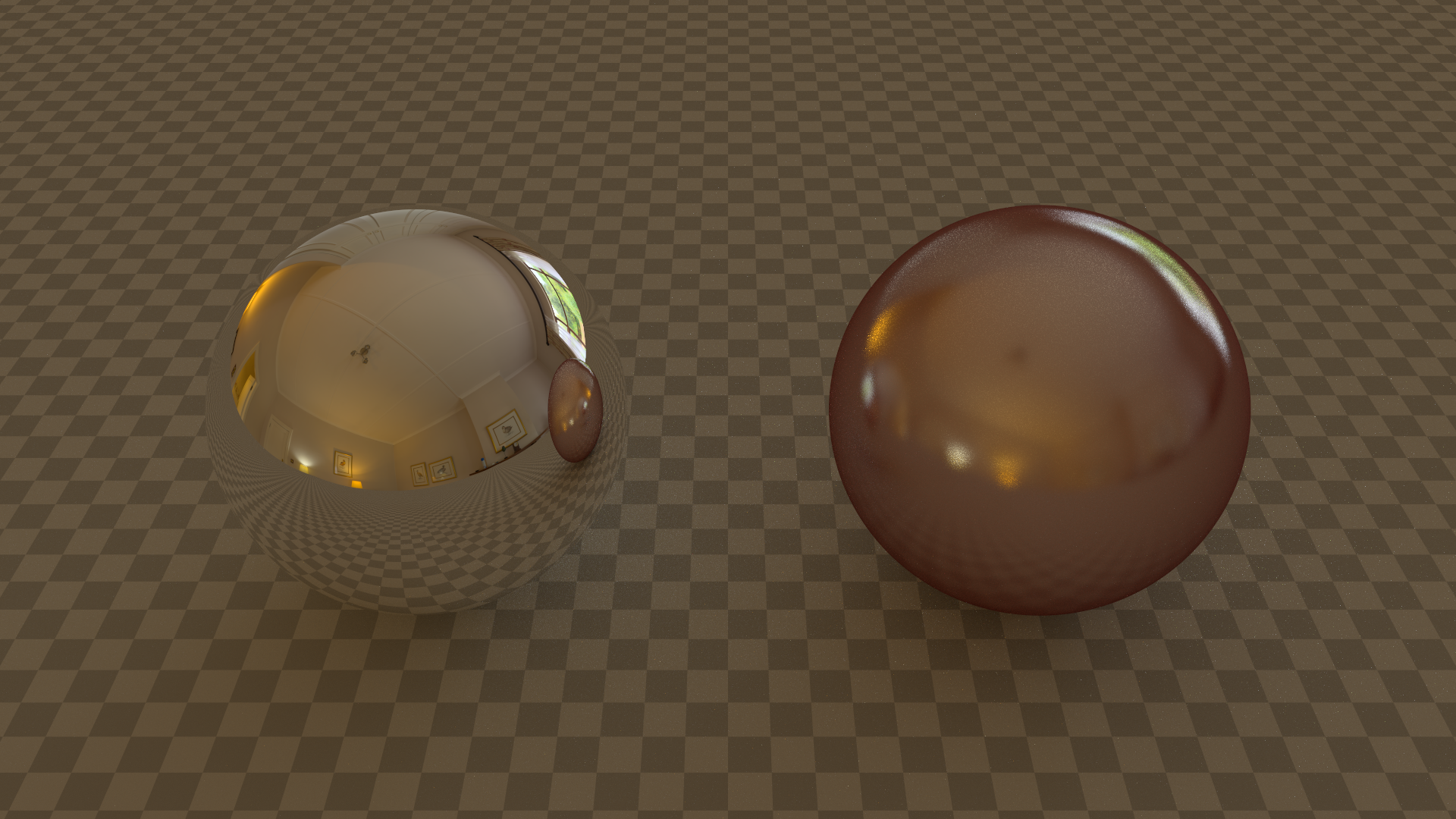
Figure 7: A scene rendered with environment maps with more evenly distributed lighting at 256 samples per pixel. For the cloudy sky map (top), $N=64$ is sufficient for good quality, and $N=128$ for the indoor map (bottom).

V Conclusion

This paper proposes an importance sampling scheme for environment maps that is independent of their parameterization, so that it works with equirectangular maps, cube maps, low distortion cube map variants, or any other parameterization of the sphere surface.

Sampling the environment map is still performed on its original parameterization so that sampling quality is unaffected and no resampling is necessary. The importance sampling scheme uses a separate map projection that is free of area distortions to simplify the necessary computations.

The granularity of importance sampling can be adapted to the environment map contents to save memory. If this adaptation is undesirable, for example if the contents of the environment map are not known in advance, the parameter $N$ can always be chosen so that the importance map resolution is similar to the resolution of the original environment map, resulting in quality and memory consumption comparable to the default choice of renderers such as Mitsuba and pbrt.

A limitation of the approach is that the bin size in the importance map is fixed and must accommodate the smallest dominant light source in the environment, resulting in bins that are smaller than necessary in homogeneous areas. This could be alleviated by using a quadtree hierarchy instead of a fixed grid, with a split criterion based on the variance of importance values inside a bin. This hierarchical approach would also entirely remove the need to choose parameter $N$.

Note that the same methods can also be applied to data given on a hemisphere, e.g. measured BRDFs, by using the hemisphere variant of the Lambert Azimuthal Equal-Area projection.

Supplementary Material

The supplementary material contains C++ code that implements the importance sampling scheme proposed in this paper in ca. 150 lines of code.

References

- [1] M. Pharr, W. Jakob, and G. Humphreys, Physically based rendering: From theory to implementation, 3rd ed. Morgan Kaufmann, 2016.
- [2] N. Greene, “Environment mapping and other applications of world projections,” IEEE Comp. Graph. and Applications, vol. 6, no. 11, pp. 21–29, Nov 1986.
- [3] M. Lambers, “Survey of cube mapping methods in interactive computer graphics,” The Visual Computer, vol. 36, no. 5, pp. 1043–1051, May 2020.
- [4] P. Clarberg and T. Akenine-Möllery, “Practical product importance sampling for direct illumination,” Computer Graphics Forum, vol. 27, no. 2, pp. 681–690, 2008.
- [5] A. Conty Estevez and P. Lecocq, “Fast product importance sampling of environment maps,” in SIGGRAPH 2018 Talks, 2018.
- [6] T. Kollig and A. Keller, “Efficient illumination by high dynamic range images,” 2002.
- [7] T. Bashford-Rogers, K. Debattista, and A. Chalmers, “Importance driven environment map sampling,” IEEE Trans. Visualization and Computer Graphics, vol. 20, no. 6, pp. 907–918, 2014.
- [8] B. Bitterli, J. Novák, and W. Jarosz, “Portal-masked environment map sampling,” Computer Graphics Forum, vol. 34, no. 4, pp. 13–19, 2015.
- [9] V. Havran, M. Smyk, G. Krawczyk, K. Myszkowski, and H.-P. Seidel, “Interactive system for dynamic scene lighting using captured video environment maps,” in Eurographics Symp. Rendering, K. Bala and P. Dutre, Eds., 2005.
- [10] S. Agarwal, R. Ramamoorthi, S. Belongie, and H. W. Jensen, “Structured importance sampling of environment maps,” in Proc. SIGGRAPH, 2003, p. 605–612.
- [11] H. Lu, R. Pacanowski, and X. Granier, “Real-time importance sampling of dynamic environment maps,” in Proc. Eurographics 2013 - Short Papers, May 2013, pp. 65–68.
- [12] J. Snyder, Map projections—a working manual, ser. Professional Paper. US Geological Survey, 1987, vol. 1395.
- [13] P. Shirley and K. Chiu, “A low distortion map between disk and square,” Journal of Graphics Tools, vol. 2, no. 3, pp. 45–52, 1997.
- [14] M. Lambers, “Mappings between sphere, disc, and square,” Journal of Computer Graphics Techniques, vol. 5, no. 2, pp. 1–21, Apr. 2016.