Topological states in chiral electronic chains

Abstract

We consider the influence of topological phases, or their vicinity, on the spin density and spin polarization through a chiral chain. We show the quantization of the Berry phase in a one-dimensional polarization helix structure, under the presence of an external magnetic field, and show its influence on the spin density. The polar angle of the momentum space spin density becomes quantized in the regime that the Berry phase is quantized, as a result of the combined effect of the induced spin-orbit coupling and the external transverse magnetic field, while the edge states do not show the polar angle quantization, in contrast with the bulk states. Under appropriate conditions, the model can be generalized to have similarities with a chain with non-homogeneous Rashba spin-orbit couplings, with zero or low energy edge states. Due to the breaking of time-reversal symmetry, we recover the effect of chiral induced spin polarization and spin transport across the chiral chain, when coupling to external leads. Some consequences of the quantized spin polarization and low energy states on the spin transport are discussed.

I Introduction

Chiral structures have attracted considerable interest. Examples are chiral magnets, chiral metals or chiral molecules, for instance in the context of chiral induced selective spin transport bauer . Molecules such as DNA or similar structures, either single stranded or doubly stranded, have been studied xie ; guo1 ; gutierrez1 ; eremko ; gutierrez2 ; gutierrez3 ; naaman ; varela ; caetano ; matityahu ; utsumi ; inui ; evers . Even though some controversy is still unresolved on a proper description of the large effect found experimentally for the spin polarization through specific chiral structures evers , there is a variety of proposals, from an effect due to the spin of the electrons xie ; guo1 ; gutierrez1 ; eremko ; gutierrez2 ; gutierrez3 ; naaman ; varela ; caetano , due to an orbital contribution liu , or due to a mixture of both utsumi . The requirement of time-reversal symmetry breaking is implemented in different ways, either through an explicit model without this symmetry (as effectively initial models considered) or through the effect of an external magnetic field, via non-unitary effects matityahu , coupling to orbital degrees of freedom utsumi or taking into account effects of interactions fransson . Synthetic structures with intrinsic or applied chiral electric fields may also be of interest.

The chiral structure may arise due to a twisting polarization (and associated twisting electric field) along the molecule, such as in the DNA-type molecule or in bent-core molecules lorman1 ; selinger ; lorman2 ; mettout1 in the context of liquid crystals. The interest is in the electronic response to the presence of this chiral structure and it may be relevant when the electronic density and mobility are significant. While in equilibrium an effect is not expected, the chiral molecule affects the spin density of a moving electron when attaching leads at the extremes of the structure.

One considers therefore an electron moving in the presence of a twisting electric field that couples to the spin and leads to a non-homogeneous spin-orbit like effect. Typically, the models considered have a gapless structure that may be changed by adding gaps to the system, either adding a magnetic field (which naturally breaks time reversal invariance and may lead to spin transport) or introducing some form of distortion of the lattice (like in the SSH model SSH ), adding local potential energy terms that separate the energies of the various lattice sites inside the unit cell of the helix-like structure.

A question that may arise is whether the considered systems may exhibit a topological nature. The change from a gapless to a gapped regime will possibly facilitate the emergence and analysis of possible topological non-trivial states. In a gapless regime, edge states are usually not found, even though exceptions have been identified in gapless critical systems Verresen ; prr3 . In a gapped regime edge states may appear, and one may wonder if signals of their presence will be felt on spin transport. One may also ask how the spin density and spin polarization are affected. The presence of the terms that lead to a gapped system, such as the addition of an external magnetic field or the lattice distortion, may change the symmetry of the problem, and the possible edge states may be zero energy modes or finite energy modes ssh1 ; ssh2 . The appearance of topology in the context of chiral molecules has been proposed before liu , including as a result of a time-dependent perturbation guo2 ; schuster .

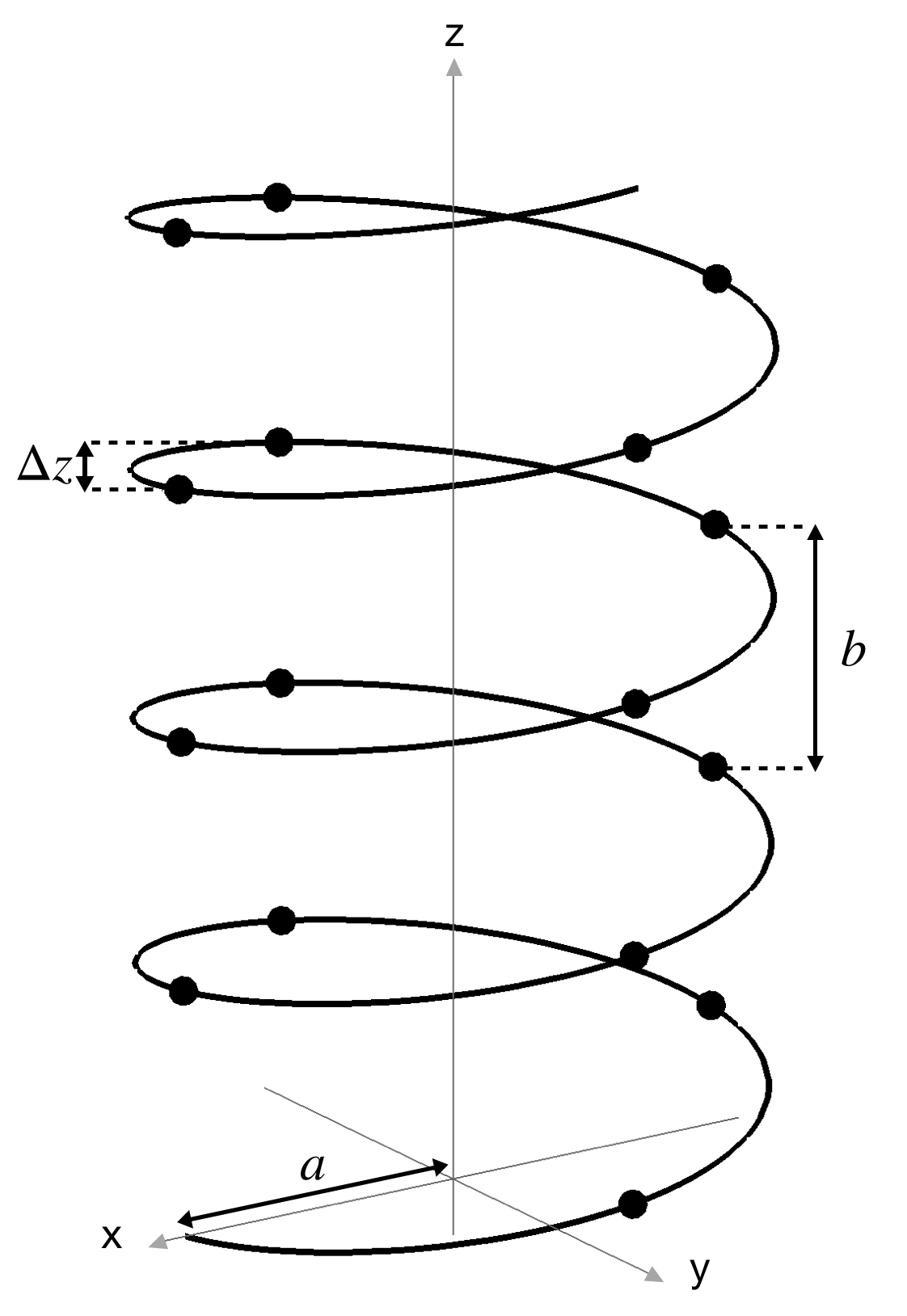
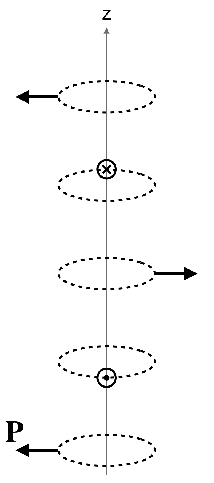
Figure 1: Schematic drawing of the three-dimensional helix structure with atoms or molecules at locations $\mathbf{r}(m,\alpha)=\left(a\cos\frac{2\pi}{\gamma}\alpha,a\sin\frac{2\pi}{\gamma}\alpha,\left[(m-1)\gamma+\alpha\right]\Delta z\right)$, along an helix of radius $a$, where $\alpha=1,\cdots,\gamma$, $b$ is the helix pitch, $\gamma$ is the number of molecules in each pitch and $m$ is an index of a given set of molecules in a given pitch. Finally, $\Delta z=b/\gamma$ is the spacing along the direction of the helix, $z$, between consecutive molecules. On the right we show a scheme of the polarization vectors taken in the plane perpendicular to the molecule axis, taking as example $\gamma=4$.

In this work we consider electronic states that propagate along a chiral chain, in a way similar to previous treatments. An example is a helix composed of molecules or atoms that display polarization and an associated electric field, $\mathbf{E}$. As an electron propagates along the helix, the electric field twists in a helical arrangement. This is, in general, a three-dimensional process. The polarization profile gives rise to an electric field that also has an helix-like structure, as shown in Fig. 1. The helix may be divided in unit cells with $\gamma$ atoms that are displaced along the axis of the helix, $z$-axis, by an amount $\Delta z=b/\gamma$, where $b$ is the helix pitch. The radius of the helix is $a$. In Fig. 1 the helix is represented for the case of $\gamma=4$.

Here, to simplify, we consider one-dimensional rods, that are immersed in the three-dimensional structure. At each molecule or atom location in a given unit cell, $m$, there is a polarization given by

$$\mathbf{P}(\alpha)=\left(P\cos\frac{2\pi}{\gamma}\alpha,P\sin\frac{2\pi}{\gamma}\alpha,0\right)$$ (1)

where $\alpha=1,\cdots,\gamma$ labels each atom within the unit cell. The problem is simplified considering an electron that moves in the direction of the axis of the helix and, therefore, we restrict its momentum to the $z$ direction. In this simplification the momentum of the electron is $\mathbf{k}=k\mathbf{e}_{z}$. Due to the presence of the electric field, the electron feels in its reference frame an effective magnetic field in the $x-y$ plane, that couples to the electron spin through a Zeeman-like effect. There is therefore a spin-orbit-like contribution to the Hamiltonian of the electron of the form $H_{SO}=\lambda\bm{\sigma}\cdot\left(\mathbf{k}\times\mathbf{E}\right)$, where $\lambda$ parametrizes the amplitude of the spin-orbit-like coupling. The chiral nature of the electric field configuration is therefore encoded in this spin-orbit term. A term like this has been shown to give rise to spin selective transport across a chiral molecule, if time reversal symmetry is broken. In this work we add an external magnetic field. We show that electronic bands arise with a gapped structure and with non-trivial quantized Berry (Zak) phases zak , under some conditions. We calculate the spin density and show some quantization of the spin density direction when the Berry phase is quantized, either taking the average of the spin density on momentum space eigenstates or taking the average over real space bulk states . In general, there are edge states of finite energy that, however, do not show spin density quantization.

We consider some generalizations of the model that give origin to additional topological zero energy edge states, in the absence of magnetic field. These are however shifted to finite, small, energies when the magnetic field is applied. It turns out that the quantization of the Zak phase is lost in some of the generalized models. The model without magnetic field or lattice distortion is topological and in class $CII$, but is gapless. Adding the lattice distortion the model is still topological and becomes gapped. Adding the magnetic field the model symmetry changes to class $C$, which is not topological in $1d$. Combining the effects of the lattice distortion and the magnetic field, the model has no time-reversal symmetry and displays finite energy edge states. The various cases will be detailed ahead. Coupling the chiral structure to external leads, a spin polarization is found considering the cases when there is time-reversal symmetry breaking. Some enhancement of the spin polarization is found at low energies due to the egde states and in the regime where the Berry phase is quantized, associated with the preferred spin density direction.

In Section II we consider a tight-binding model with spin-orbit coupling and external magnetic field and study its energy spectrum and symmetries, calculate the Berry phase of the energy bands and determine the conditions for its quantization. In Section III we calculate the momentum space spin density and associate a quantization property with the quantization of the Berry phase. In Section IV a real-space description is adopted to determine the edge states and the real space spin density. In Section V we consider some generalizations of the model that lead to zero energy or low energy edge modes. In Section VI we study the spin transport along the system, coupling the chain to leads.

II Energy bands and Berry phase in a one-dimensional chiral structure

We consider a tight-binding model for the motion of the electrons. The spin-orbit coupling leads to a term that has to be symmetrized appropriately gutierrez1 ; gutierrez2 ; pareek . The Hamiltonian in real space is chosen to be

$$H = \sum_{j}\sum_{m_{s}}c_{j,m_{s}}^{\dagger}\left(-\mu+\mu(j)\right)c_{j,m_{s}}$$ (6)

$$- \sum_{j}\sum_{m_{s},m_{s}^{\prime}}c_{j,m_{s}}^{\dagger}\left(\mathbf{B}\cdot\bm{\sigma}_{m_{s},m_{s}^{\prime}}\right)c_{j,m_{s}^{\prime}}$$

$$- w\sum_{j}\sum_{m_{s}}\left(c_{j,m_{s}}^{\dagger}c_{j+1,m_{s}}+c_{j+1,m_{s}}^{\dagger}c_{j,m_{s}}\right)$$

$$- \lambda\sum_{j}\left(c_{j+1,\uparrow}^{\dagger},c_{j+1,\downarrow}^{\dagger}\right)\left(\begin{array}[]{cc}0&\chi_{j}\\ -\chi_{j}^{*}&0\end{array}\right)\left(\begin{array}[]{c}c_{j,\uparrow}\\ c_{j,\downarrow}\end{array}\right)$$

$$- \lambda\sum_{j}\left(c_{j,\uparrow}^{\dagger},c_{j,\downarrow}^{\dagger}\right)\left(\begin{array}[]{cc}0&-\chi_{j}\\ \chi_{j}^{*}&0\end{array}\right)\left(\begin{array}[]{c}c_{j+1,\uparrow}\\ c_{j+1,\downarrow}\end{array}\right)$$ (11)

where $c_{j,m_{s}}=c_{m,\alpha,m_{s}}$ destroys an electron at site $j$ and with spin projection $m_{s}$. Here $j=(m-1)\gamma+\alpha$ labels each molecule or atom location, in cell $m$ and location $\alpha$ within the cell, $\mu$ is the chemical potential, $w$ is the hopping amplitude to a nearest neighbor location, $m_{s}=\uparrow,\downarrow$ are the spin projections and $\chi(j)=iE_{y}(j)-E_{x}(j)=-Ee^{-i\Phi(j-1)}$ has a constant amplitude and where $\Phi=(2\pi)/\gamma$. ($\mu,w,B,\lambda E$ have energy units). The amplitude of the electric field is taken as $E=\sqrt{E_{x}^{2}+E_{y}^{2}}=1$. Also, we have added a local external magnetic field, $\mathbf{B}$, that couples to the spin density of the electrons. This term explicitly breaks time reversal invariance and allows the opening of gaps between the bands. Also, it allows the study of the effect of time-reversal symmetry breaking on a multiband fermionic system ssh2 .

If the chiral chain is finite the electric field amplitude is not a constant. In order to simplify the problem we consider a long chain and neglect the effect of the ends of the chain by considering a constant amplitude throughout. We take $w=1,\mu=0$. Also, in a more realistic model there is coupling between sites $j$ and $j+\gamma$, which we neglect here, as well as the three-dimensional motion of the electrons along the structure. In addition, we consider a simplified model of one orbital state in which the hopping term is a constant and consider that the effect of the twist along the helix only affects the spin-orbit term gutierrez1 ; gutierrez3 .

The effects of a spin-orbit interaction in multiband systems have been extensively studied in the context of topological insulators hasan ; zhang ; kane focusing mainly on homogeneous spin-orbit terms. Non-homogeneous (or modulated) spin-orbit terms have also been considered such as due to a curved wire gentile or in the generalized Aubry-André class malard . Here we focus on a spin-orbit interaction that encodes the chirality of the polarization or electric field configuration.

The explicit construction of the states is obtained diagonalizing the Hamiltonian in real space for a finite helix using open boundary conditions, giving both the bulk states and edge states. Considering an infinite helix we may use a momentum space description, with a basis of size $\gamma$. The Hamiltonian in momentum space is a $(\gamma\times 2)\times(\gamma\times 2)$ matrix that gives rise to $\gamma\times 2$ electronic bands. In the case of $\gamma=2$ the electric field has a staggered structure and so we consider higher values of $\gamma$.

Let us consider explicitly, as an example, the case of $\gamma=4$. In this case the Hamiltonian matrix in momentum space is written in a basis of vectors $(1\uparrow,1\downarrow,3\uparrow,3\downarrow,2\uparrow,2\downarrow,4\uparrow,4\downarrow)^{T}$. Considering that in this case

$$\chi=(-E,iE,E,-iE)$$ (12)

and defining $Z_{ijk}=\sigma_{i}\otimes\sigma_{j}\otimes\sigma_{k}$, we can write the Hamiltonian matrix as

$$H(k) = -wZ_{100}-\frac{w}{2}\left(1+\cos k\right)Z_{110}$$ (13)

$$- \frac{w}{2}\left(1-\cos k\right)Z_{220}-\frac{w}{2}\sin k\left(Z_{120}+Z_{210}\right)$$

$$+ \lambda E\left(Z_{232}-\frac{1}{2}Z_{121}+\frac{1}{2}Z_{211}\right)$$

$$+ \frac{\lambda E}{2}\left(\sin k\left(Z_{111}-Z_{221}\right)-\cos k\left(Z_{121}+Z_{211}\right)\right)$$

$$- \left(B_{x}Z_{001}+B_{y}Z_{002}+B_{z}Z_{003}\right)$$

II.1 Symmetries

The Hamiltonian matrix has some symmetries. Consider for instance the case of $\gamma=4$. In this case the Hamiltonian has particle-hole (or charge conjugation) symmetry, defined by an operator, $C$, that satisfies $CH^{*}(-k)C^{\dagger}=-H(k)$, which yields $C=\left(\sigma_{3}\otimes\sigma_{0}\otimes\sigma_{2}\right)$. Since $C^{T}=-C$ the model is in class C, which in one dimension is predicted to be non-topological schnyder . If the external magnetic field is absent, $\mathbf{B}=0$, then the system also has time reversal symmetry, $TH^{*}(-k)T^{\dagger}=H(k)$, with $T=\left(\sigma_{0}\otimes\sigma_{0}\otimes\sigma_{2}\right)$ and chiral symmetry, $OH(k)O^{\dagger}=-H(k)$, with $O=\left(\sigma_{3}\otimes\sigma_{0}\otimes\sigma_{0}\right)$. In this case the model is in class CII and in one dimension is predicted to be a class $Z$ topological system. Note that the model is gapless in this case.

In addition to the global symmetries considered, the Hamiltonian in real space also has a spatial symmetry, in some conditions. Defining a transformation of the fermion operators as

$$c_{j,m_{s}}\rightarrow c_{j+1,m_{s}}e^{im_{s}\frac{\pi}{\gamma}}$$ (14)

the spin-orbit term and the hopping term remain invariant. Including an external magnetic field along the $z$ direction also leaves the Hamiltonian invariant (under periodic boundary conditions). However, the $B_{x}$ and $B_{y}$ components do not remain invariant. The term due to $B_{x}$ transforms as

$$c_{j,\uparrow}^{\dagger}B_{x}c_{j,\downarrow}+c_{j,\downarrow}^{\dagger}B_{x}c_{j,\uparrow}\rightarrow c_{j,\uparrow}^{\dagger}B_{x}c_{j,\downarrow}e^{-i\frac{2\pi}{\gamma}}+c_{j,\downarrow}^{\dagger}B_{x}c_{j,\uparrow}e^{i\frac{2\pi}{\gamma}}$$ (15)

and the term due to $B_{y}$ transforms as

$$c_{j,\uparrow}^{\dagger}(-iB_{y})c_{j,\downarrow}+c_{j,\downarrow}^{\dagger}(iB_{y})c_{j,\uparrow}$$

$$\rightarrow c_{j,\uparrow}^{\dagger}(-iB_{y})c_{j,\downarrow}e^{-i\frac{2\pi}{\gamma}}+c_{j,\downarrow}^{\dagger}(iB_{y})c_{j,\uparrow}e^{i\frac{2\pi}{\gamma}}$$ (16)

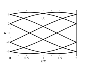
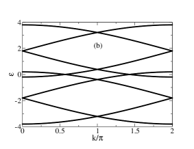
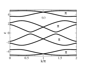
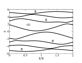
Figure 2: Energy bands for a) $\lambda=2$ and no external magnetic field, b) no spin-orbit coupling and $B_{x}=1,B_{y}=0,B_{z}=1.5$, c) $\lambda=2$ and $B_{x}=1,B_{y}=B_{z}=0$ and d) with spin-orbit coupling $\lambda=2$ and $B_{x}=1,B_{y}=0,B_{z}=1.5$. In panels c) and d) we show the bands with non-trivial Berry phase, $\pi$ phase. In panel d) the bands are all separated and the Berry phase is for each band individually. The bands have either a $\pi$ Berry phase or a Berry phase of zero. In panel c), since the bands have degenerate points, the Berry phases indicated are for groups of two bands. In panels a) and b) the Berry phases are not quantized and have arbitrary real values.

II.2 Berry phase

In the case of bands with a finite gap between them, the Berry phase may be easily determined. In general, a Berry phase does not have a topological nature. However, the presence of some symmetries, like inversion, chiral or charge conjugation symmetries zak ; benalcazar , ensures a quantization of the Berry phase. This is calculated $mod(2\pi)$ and a trivial band has zero Berry phase and a topological band has a Berry phase of $\pi$. The Berry phase of a given band may be calculated in a standard way niu ; resta ; fukui ; benalcazar . One divides the Brillouin zone considering $N$ discrete points, $k\in[0,2\pi]$, with momenta taking the values $k_{1},\cdots,k_{N}$. The band’s Berry phase $\gamma_{B}$ may be obtained defining the link variable $U(k_{l})=\varphi^{*}(k_{l})\varphi(k_{l+1})$, and summing over $k_{l}$ as

$$\gamma_{B}=-i\sum_{l}\log U(k_{l})$$ (17)

where $\varphi(k_{l})$ are the eigenstates of the Hamiltonian in momentum space.

This procedure can be generalized if there are degenerate points between the bands taking a link variable as $U(k_{l})=det\mathbf{U}(k_{l})$, involving the determinant of the matrix

$$\mathbf{U}_{ij}(k_{l})=\varphi_{i}^{*}(k_{l})\varphi_{j}(k_{l+1})$$ (18)

where $1\leq i,j\leq N$ run over the eigenstates and $\varphi_{i}(k_{l})$ is the eigenstate at momentum $k_{l}$ of the $i$th band.

In Fig. 2 we show the energy bands and non-trivial (quantized) Berry phases, considering a unit cell with four sites, $\gamma=4$. With no spin-orbit coupling (zero electric field) or zero external magnetic field, the bands are gapless (as shown in Fig. 2(a),(b) ) and the Berry phases are not quantized. Combining the two effects, in some regimes gaps appear between the various bands. The charge-conjugation symmetry implies that there are pairs of states that are related by $\epsilon_{n}(k)\rightarrow-\epsilon_{m}(-k)$, where $n,m$ are two bands. In Fig. 2(c) we consider the addition of a magnetic field along the $x$ direction. Some gaps appear and the bands appear in groups of two. The sum of the Berry phases of the two lowest bands adds to $\pi$ as well as the sum of all following pairs of bands. We show in Fig. 2(d) an example of a situation where the various bands are separated by finite gaps as a result of adding a magnetic field $B_{z}$ different from zero. The results for the Berry phases show that some bands are trivial and four bands are non-trivial, with a Berry phase $\gamma_{B}=\pi$. Note that the Berry phases of all the bands below zero energy add to zero, as a consequence of the charge-conjugation symmetry. Also, even though the model is in class $C$, which is not topological in the usual scheme, the Berry phases of individual bands show quantization properties.

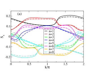
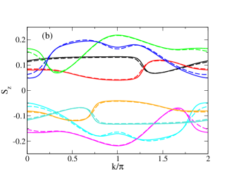
Figure 3: Spin density averages $S_{x}$ and $S_{z}$, as a function of momentum, for each band for $\gamma=4$, for a trivial case (dashed lines) and a case with quantized Berry phase (solid lines). The case of quantized Berry phase has parameters $\lambda=2,B_{x}=1.2,B_{y}=0,B_{z}=1.5$ and the trivial case has the same parameters except $B_{y}=0.5$.

As mentioned above, the quantization of Berry phase may result from inversion symmetry, chiral symmetry or charge-conjugation symmetry benalcazar . The helix structure and the presence of a magnetic field along $x$ and $z$ directions implies no inversion symmetry. In the presence of a magnetic field, $\mathbf{B}\neq 0$ there is no chiral symmetry. However, there is a hidden symmetry if $B_{y}=0$ (for $\gamma=4$). It is of the type $Oh(k)O^{-1}=-h(-k)$, and may se seen as a combination of inversion symmetry $Ih(k)I^{-1}=h(-k)$ and chiral symmetry $\Pi h(k)\Pi^{-1}=-h(k)$ specifically $O=\sigma_{2}\otimes\sigma_{1}\otimes\sigma_{2}$. The various symmetries chiral symmetry, hidden symmetry and charge-conjugation symmetry also only hold if the chemical potential vanishes and the number of occupied bands equals the number of unnoccupied bands. There is a relation between the Zak phase, the electric polarization (dipole moment) and Wilson loops vanderbilt ; resta2 ; niu ; benalcazar . Using the symmetry properties of the Wilson loops and its relation to the dipole moment, $p$, benalcazar as the sum of the eigenvalues of the Wilson loop via the Wannier centers (phases of the eigenvalues of the Wilson loop), it can be shown that, in the presence of inversion symmetry, the dipole moment (normalized to $1$) of the states summed over the occupied bands, satisfies $p_{occ}=-p_{occ}$ implying that it is quantized to $0,1/2$, which leads to a Zak phase of $0,\pi$. A similar analysis if there is a chiral symmetry leads to the result that $p_{occ}=p_{unnocc}$, since the chiral symmetry connects states with positive energy with states with negative energy. Using the general result that $p_{occ}+p_{unnocc}=0$ (summing over all bands topology is trivial) we get the same result that $p_{occ}=-p_{occ}$ and, therefore, it is quantized. A similar result may be shown for charge-conjugation symmetry benalcazar . In the case of the hidden symmetry we get that $p_{occ}=-p_{unnocc}$ since this symmetry changes the sign of the momentum and relates the positive energy states with the negative energy states. So, at first sight, no conclusion about the quantization may be obtained. At zero chemical potential the charge-conjugation symmetry is present (even in the presence of a magnetic field) and there is quantization of the Berry phase, considering the sum over the occupied bands. Indeed, we find, by explicit calculation of the Berry phases, that the sum over the lower four bands always leads to a zero Berry phase. It is quantized but topologically trivial. This is consistent with the class $C$, which is not topological in $1d$. As mentioned above, if $B_{y}=0$ we find that some of the bands, or groups of bands, show a quantized $\pi$ Berry phase. Adding $B_{y}\neq 0$ all the bands show non-quantized Berry phases, but are such that the sum over the occupied bands still yields a quantized, vanishing Berry phase, as imposed by the charge-conjugation symmetry. Even though the charge-conjugation and the hidden symmetry only hold if the chemical potential vanishes, it turns out that a finite chemical potential placed in a gap between the bands leads to a Berry phase of each band that is the same as for $\mu=0$. As a consequence, it is possible to select the chemical potential such that the sum of the Berry phases over the set of occupied bands is topologically non-trivial and quantized to $\pi$. This only takes place if $B_{y}=0$, and therefore we argue that the quantization of the Berry phase is associated with the hidden symmetry, since the charge-conjugation symmetry implies $p_{occ}=p_{unnocc}$ and the hidden symmetry implies $p_{occ}=-p_{unnocc}$.

The non-trivial Berry phase found for $\gamma=4$ can be generalized to any number of points in the unit cell. Recalling that in the rest frame of an electron the effect of the electric field can be seen as an effective magnetic field, $\mathbf{b}$, that couples to the electron spin via a Zeeman coupling, we can see that the effective field has components $\mathbf{b}\sim(-E_{y},E_{x},0)$. We can see that at site $j$ of the unit cell, $b_{y}/b_{x}=-1/\tan[\Phi\left(j-1\right)]$, with $\Phi=2\pi/\gamma$. We have found that the condition for a non-trivial Berry phase can be obtained selecting

$$\frac{B_{y}}{B_{x}}=\frac{1}{\tan\Phi}$$ (19)

In a more general case, for which

$$\frac{E_{y}}{E_{x}}=\tan\left(\Phi+\delta_{1}\right)$$ (20)

with $\delta_{1}$ any phase, we find that the Berry phase is quantized if we take

$$\frac{B_{y}}{B_{x}}=\frac{1}{\tan\left(\Phi+\delta_{2}\right)}$$ (21)

with $\delta_{2}=-\delta_{1}\pm l\pi$, with $l$ an integer.

We also find regimes of quantized Berry phases for a model of spinless electrons but with a non-trivial hopping structure, due to the presence of more than one orbital state, and considering both nearest neighbor and next-nearest neighbor terms (with a complex part) and therefore an external magnetic field is not required. This is shown in Appendix A.

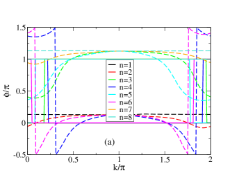
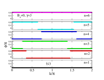
Figure 4: a) Comparison of polar angle of spin density average over an eigenstate of momentum $k$ and band $n$, between a trivial case (dashed lines) and a non-trivial (quantized Berry phase) case (solid lines), as a function of momentum, for the various bands. The parameters are the same as in Fig. 3. b) Comparison for $\gamma=4$ of the polar angles for the various bands for $B_{z}=1.5$ and $B_{z}=0$. c) Polar angle for $\gamma=3$ for $B_{z}=0$.

III Momentum space spin density and polar angle quantization

The spin density operator components may be defined by

$$S_{\beta}(k)=\frac{1}{\gamma}\sum_{\alpha=1}^{\gamma}\sum_{m_{s},m_{s}^{\prime}}c^{\dagger}(k,\alpha,m_{s})\sigma_{m_{s},m_{s}^{\prime}}^{\beta}c(k,\alpha,m_{s}^{\prime})$$ (22)

where $\beta=x,y,z$ and $\sigma^{\beta}$ are Pauli matrices. We may consider the average value of these operators in the eigenstates of the Hamiltonian, for a given band and momentum value. That is, we consider for a given momentum value and energy band, $n$,

$$\langle S_{x}(k,n)\rangle = \frac{1}{\gamma}\sum_{\alpha=1}^{\gamma}\left(u_{n}^{*}(k,\alpha,\uparrow)u_{n}(k,\alpha,\downarrow)\right.$$

$$+ \left.u_{n}^{*}(k,\alpha,\downarrow)u_{n}(k,\alpha,\uparrow)\right)$$

$$\langle S_{y}(k,n)\rangle = \frac{1}{\gamma}\sum_{\alpha=1}^{\gamma}\left(-iu_{n}^{*}(k,\alpha,\uparrow)u_{n}(k,\alpha,\downarrow)\right.$$

$$+ \left.iu_{n}^{*}(k,\alpha,\downarrow)u_{n}(k,\alpha,\uparrow)\right)$$

$$\langle S_{z}(k,n)\rangle = \frac{1}{\gamma}\sum_{\alpha=1}^{\gamma}\left(|u_{n}(k,\alpha,\uparrow)|^{2}-|u_{n}(k,\alpha,\downarrow)|^{2}\right)$$

where $u_{n}(k,\alpha,m_{s})$ is the eigenfunction of state $n,k,\alpha,m_{s}$. We may also define, for each momentum value and energy band, the normalized spin vector

$$\hat{S}_{n}(k)=\frac{\left(\langle S_{x}(k,n)\rangle,\langle S_{y}(k,n)\rangle,\langle S_{z}(k,n)\rangle\right)}{\sqrt{\langle S_{x}(k,n)\rangle^{2}+\langle S_{y}(k,n)\rangle^{2}+\langle S_{z}(k,n)\rangle^{2}}}$$ (24)

with a direction in space parametrized by the spherical coordinate angles $(\theta(k,n),\phi(k,n))$. We will show that when the Berry phase is quantized, the polar angle gets quantized as a function of momentum.

In Fig. 3 we show the results for the spin density average as a function of momentum for the various bands for a unit cell of four sites. We consider the spin densities along the $x$ and $z$ directions. Also, we compare the results for a system which shows a quantized Berry phase and one which is not quantized. The results are in general similar, since the trivial regime is obtained adding a small magnetic field along the $y$ direction. However, if we consider the polar angle for the same two cases, we show in Fig. 4 that in the quantized Berry phase regime, the polar angle also becomes quantized, while in the trivial case it is in general not quantized. This result holds for any unit cell size, $\gamma$. The angle with respect to the $z$ axis shows no quantization.

Table 1: Quantized Berry phase, $\gamma_{B}$, and polar angle, $\phi(k,n)$, for the cases of $\gamma=3,4,5,6$, when the conditions of eq. (19) are met. Here $k$ is the momentum and $n$ is the band index, $n=1,\cdots,2\gamma$.

$\gamma=3$			$\gamma=4$			$\gamma=5$			$\gamma=6$
n	$\gamma_{B}$	$\phi(k,n)/\pi$	n	$\gamma_{B}$	$\phi(k,n)/\pi$	n	$\gamma_{B}$	$\phi(k,n)/\pi$	n	$\gamma_{B}$	$\phi(k,n)/\pi$
1	$\pi$	-1/6	1	$\pi$	0	1	$\pi$	1/10	1	$\pi$	1/6
2	0	5/6,-1/6	2	0	0	2	0	1/10	2	0	1/6
3	$\pi$	-1/6,5/6	3	$\pi$	0, 1	3	0	1/10,11/10	3	$\pi$	1/6
4	$\pi$	-1/6,5/6	4	0	1,0	4	$\pi$	11/10,1/10	4	0	7/6,1/6
5	0	5/6,-1/6	5	0	0,1	5	0	1/10,11/10	5	0	1/6,7/6
6	$\pi$	5/6	6	$\pi$	1,0	6	0	1/10,11/10	6	0	1/6,7/6
			7	0	1	7	$\pi$	11/10,1/10	7	0	7/6,1/6
			8	$\pi$	1	8	0	1/10,11/10	8	0	7/6,1/6
						9	0	11/10	9	0	1/6,7/6
						10	$\pi$	11/10	10	$\pi$	7/6
									11	0	7/6
									12	$\pi$	7/6

In Fig. 3 and in Fig. 4(a) we consider the case where $B_{z}\neq 0$. This was chosen earlier since applying a magnetic field in the parallel and transverse directions, with respect to the chiral axis, allows a simplified problem where all bands are separated by gaps. As shown in Fig. 2(c), turning off $B_{z}$ leads to the closing of some gaps, even though a quantized Berry phase is still found for groups of two bands. Turning off $B_{z}$ we find that the polar angle is also quantized. In Fig. 4(b) we compare the cases of $B_{z}=1.5$ and $B_{z}=0$, for $\gamma=4$, which shows the quantization in both cases. In Fig. 4(c) we show the quantization of the polar angle for $\gamma=3$ when $B_{z}=0$. The case of vanishing $B_{z}$ will be considered later in the spin transport across the helix.

We summarize the results for the Berry phase, $\gamma_{B}$, and the polar angle, $\phi(k,n)/\pi$, for each band, $n$, in Table I for $\gamma=3,4,5,6$ and $B_{z}=1.5$. We see that for the lowest energy levels the spin density is aligned along $\mathbf{B}$ while for the higher levels the spin density is aligned along the $\mathbf{B}+\pi$ direction. In the intermediate levels the spin density is aligned in one or the other direction depending on the momentum value, $k$. There is a competition between the external magnetic field and the effective field that is the result of the electric field of the helix. In the non-quantized cases this leads in general to a polar angle that varies with the momentum and band, while in the quantized Berry phase cases the polar angle has plateaus. In some cases the competition between the two magnetic fields leads to a situation where for a given band there is only one plateau. This happens for the lowest and/or the highest energy bands.

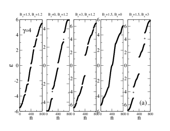
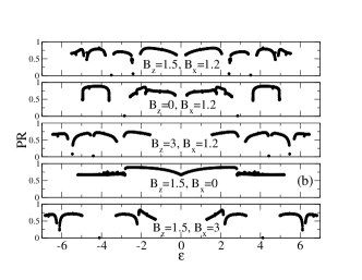
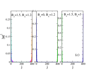
Figure 5: Real space diagonalization with open boundary conditions for a finite system of 100 unit cells. a) Comparison of energy values for $\gamma=4$ and different values of the external magnetic field, where $n$ is the level label. b) Corresponding results for the participation ratio of each energy state. c) Absolute value of the eigenfunctions of the edge states as a function of space location, $j$, for some values of the magnetic field.

IV Real space description and edge states

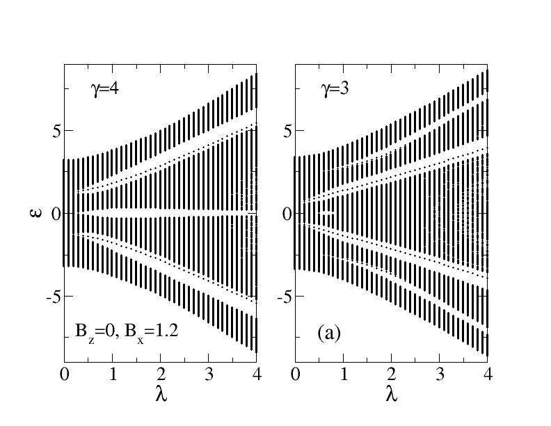
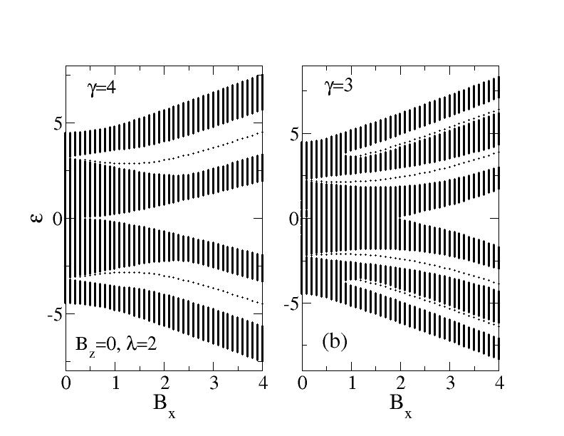
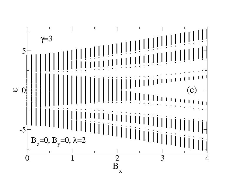
Figure 6: Comparison of energy values for $\gamma=4$ and $\gamma=3$ as a function of a) $\lambda$ and b) $B_{x}$, for the quantized Berry phase and c) for $\gamma=3$ with $B_{y}=0$ (non-quantized case).

The presence in some regimes of a quantized Berry phase may suggest the presence of edge states at the ends of the helix. These are revealed diagonalizing the Hamiltonian in real space and considering open boundary conditions. The results are shown in Fig. 5. In the top panel we show the energy levels for similar parameters as those taken in Fig. 2 with $\lambda=2$ and $B_{x}=1.2,B_{y}=0,B_{z}=1.5$, together for other values of the magnetic field. There are states inside the gaps, but there are no zero energy states. In non-chiral multiband systems the Zeeman term has a similar effect ssh2 ; bahari . Recall that the sum of the Berry phases of the bands below zero energy is zero, consistently with no edge states in the gap surrounding zero energy. The states inside the gaps are well localized, as shown in Fig. 5(b) by the participation ratio of each level and by the wave functions shown in Fig. 5(c), that are well localized at the edges of the chain. The participation ratio for a given state is defined as

$$PR=\frac{L^{-1}}{\sum_{j}\left(|\psi_{j}|^{2}\right)^{2}}$$ (25)

where $|\psi_{j}|^{2}$ includes the sum over the two spin components at site $j$. It is such that is of the order of one if the state is extended and is of the order of $1/L$, where $L$ is the system size, if the state is localized. We may argue that the edge states appear in cases where the sum of the Berry phases below a given gap is non-trivial (this is particularly clear in the case that $B_{z}=0$), as would be expected, even though the model is in class $C$. Even though this picture seems appealing, it turns out that the edge states remain in some cases, even when the Berry phase is not quantized to zero or $\pi$. The momentum space band structure and the energy states for the finite system agree qualitatively, but the boundary conditions used are not the same. Also, unless the indirect gaps between the bands are positive, the possible edge (localized) states merge into the continuum, are not seen and become extended, as revealed for instance by the absence of small PRs.

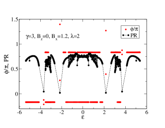
Figure 7: Participation ratio and spin polar angle for the energy states of a chain with unit cell with $\gamma=3$, with a finite size of 100 cells and using open boundary conditions, for $B_{z}=0,B_{x}=1.2,\lambda=2$ in the topological case with $B_{y}/B_{x}=1/\tan\Phi$. The polar angle of the bulk states is quantized along the direction of the magnetic field in the transverse plane and along the opposite direction. Note that the polar angle is not quantized when we consider the edge states, for which the participation ratio has large drops.

In the top two panels of Fig. 6 we show the dispersion of the localized edge states as a function of $\lambda$ and $B_{x}$ for $\gamma=3,4$, in regimes where the Berry phase is quantized. In Fig. 6(c) we consider a similar plot of the energy levels for $\gamma=3,B_{z}=0,\lambda=2$ but taking $B_{y}=0$, which can be shown in momentum space to lead to a phase with a non-quantized Berry phase and a non-quantized spin polar angle. But, as clearly shown, edge states are found inside the various gaps, and these states are well localized at the edges of the system.

As in the case where the spin operators were averaged over the momentum space eigenstates, we also find for the bulk states of the finite system a quantization of the spin polar angle (in the topological regimes). This contrasts with the result that the edge states do not display this quantization. This is shown in Fig. 7 where the polar angle of each eigenstate is shown, together with the participation ratios, for $\gamma=3$. While the bulk states display the expected quantization, the edge states, identified by the small participation ratios, do not lead to a quantized polar angle.

V Generalized models: lattice distortion and Rashba spin-orbit

It is interesting to consider generalizations of the model. We may consider that along the helix some dimerization, trimerization, etc, may occur, that leads to a non-homogeneous set of hopping terms between the various neighbors. For instance, a unit cell with two sites, $\gamma=2$, which may be dimerized, or a unit cell with $\gamma=3$ which may be trimerized in some way. The first case is similar to a SSH model (with spin added). The model by itself has a topological regime, with zero energy edge states, quantized winding number and quantized Berry phase.

For instance, taking $\gamma=2$, if the two hoppings $t_{1},t_{2}$ are not equal, topology emerges if $t_{2}>t_{1}$. Including spin in a SSH model, the bands become degenerate, but considering a magnetic field along the direction of the chain, $B_{z}\neq 0$ lifts the degeneracy and one finds the expected topological bands with $\pi$ Berry phase. Adding the spin-orbit term that results from the chiral structure, the topology is maintained, and due to the spin-orbit coupling a transverse spin density along the $y$ direction is found. This leads naturally to a quantization of the polar angle along either $\phi=\pi/2$ or $3\pi/2$.

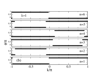
Figure 8: a) Energy bands of a chain with $\gamma=3$ and non-homogeneous hoppings, with $t_{1}=t_{2}=1,t_{3}=2$, for different values of spin-orbit coupling $\lambda=0,0.1,1$. b) Quantization of the polar angle as a function of momentum, for topological case, for each band, for $\gamma=3$ and $\lambda=1$.

Taking $\gamma=3$ and selecting the three hoppings such that $t_{3}>t_{1},t_{2}$, a non-trivial quantized spin polar angle is found. Unexpectedly, for $t_{3}<t_{1},t_{2}$ a quantized polar angle is also found, even though the Berry phase vanishes (as expected for a trivial regime of a trimerized band). If $t_{1}=t_{2}=t_{3}$ there is no induced spin density in the transverse directions and therefore there is no quantization of the polar angle, since it is ill-defined. These results are shown in Fig. 8 where we show the topological bands and the quantization of the polar angle when the spin-orbit term is present. The spin-orbit coupling induces a transverse spin density and a quantization of the polar angle, even without the presence of an external transverse magnetic field (a field along $z$ splits the bands). If $t_{3}\neq t_{1}=t_{2}$, we get in general non-trivial Berry phases, if a spin-orbit coupling term is present. In Fig. 9 we show the Berry phase (normalized by $2\pi$) as a function of $t_{3}i$ and $\lambda$, for zero transverse magnetic field but with $B_{z}$ finite, showing the regimes where a non-trivial phase is found.

Figure 9: Berry phase of the combined two lowest energy levels, as a function of $t_{3},\lambda$, for $B_{x}=B_{y}=0,B_{z}=1.5$, for $t_{1}=t_{2}=1$. The Berry phase of the lowest level is non-trivial for $t_{3}>1$ and the Berry phase of the second level is non-trivial when $t_{3}<1$ and $\lambda$ is large enough.

The spin-orbit coupling term acts as an effective non-local magnetic field (depends on momentum), and tends to align the spin density. With $t_{3}=t_{1}=t_{2}$ the spin-orbit coupling does not lead to non-trivial Berry phases, unless we add an external transverse magnetic field with the appropriate direction. With $\lambda=0$ the addition of a field $B_{x}\neq 0$ (and $B_{y}$ satisfying the quantization condition, Eq. (19)), also leads to a quantized non-trivial Berry phase if $t_{3}>t_{1},t_{2}$. With $t_{3}\neq t_{1}=t_{2}$, and with the spin-orbit term, we get in general an alignment of the spin density.

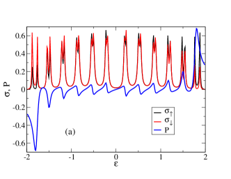
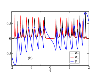
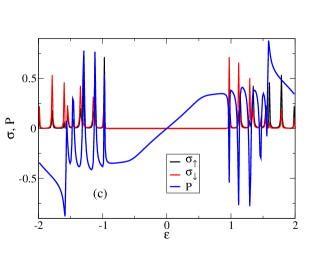
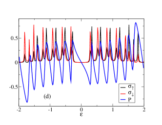
Figure 10: Differential conductances for an incident electron with spin $\uparrow$ and an incident electron with spin $\downarrow$ and spin polarization, for $\gamma=4$, $10$ unit cells, $V=0.5,\lambda=2,B_{z}=0$ for a) $B_{x}=0.5,B_{y}=0,\lambda_{R}=0$, b) $B_{x}=1,B_{y}=0,\lambda_{R}=0$, c) $B_{x}=1,B_{y}=0,\lambda_{R}=2$ and d) $B_{x}=1,B_{y}=0.2,\lambda_{R}=0$.

We remark, however, that there is no spin polarization in spin transport if $\mathbf{B}=0$ since time reversal is preserved, even though a spin density is created as a consequence of the spin-orbit coupling. The spin density of an incoming spin up or spin down electron is rotated, but in such a way that there is no difference between the two incoming electrons.

A related model with time reversal symmetry has been considered malard that includes Rashba, $\lambda_{R}$, and Dresselhaus, $\lambda_{D}$, spin-orbit couplings. The Dresselhaus is uniform and the Rashba has a constant term plus a modulated one, that can be argued to be in the class of a generalized Aubry-André-Harper model. There are several phases with winding number (chiral symmetry) and gapless critical surfaces/lines and zero energy states. Inspired by these results we consider adding to the expression for $\chi(j)$ of our model Eq. 11 a constant $-E_{y}$ term, independent of the site, $j$, and a Rashba-like term that results from a constant $E_{x}$. Adding for instance a spatially uniform Rashba-like term, with an amplitude $\lambda_{R}$, leads to some consequences that will be explored in the next section. If $\lambda$ and $\lambda_{R}$ are not simultaneously small, one finds zero energy states if there is no external magnetic field. A term that may originate from a uniform electric field along $-y$, may be considered with an amplitude $\lambda^{\prime}$. In the case of zero external magnetic field and $\gamma=4$, the spectrum remains gapless around zero energy if $\lambda_{R}=\lambda^{\prime}$ but there are two gaps between bands two and three and between bands six and seven. If $\lambda_{R}\neq\lambda^{\prime}$ a gap opens around zero energy. If $\lambda_{R}>\lambda^{\prime}$ there are edge states inside the three gaps with the appearance of zero energy states. Applying an external magnetic field the zero energy states turn into finite energy but are still well localized on the edges of a finite system, if the magnetic field is small enough.

Terms of the type of a SSH model lead to zero energy states, in addition to the finite energy edge states found in the helix problem. The model with Rashba coupling malard also leads to zero energy states (if $B=0$). Adding $B_{x}$, the zero energy states in the gap acquire a small finite energy, but the states remain in the gap that is centered around zero energy. These states may contribute to either the low energy conductance or spin response when the system is coupled to external leads. A significant effect is found if there is a small coupling to the leads and a not too small or too large system (see for instance, dong ; balabanov ). This will be considered next.

VI Spin transport along a chiral chain

VI.1 Scattering states

Let us now determine the possible influence of the topological states on the spin transport along the chain. We consider two leads that are attached to the chiral chain. We may inject a spin up or spin down electron from the left lead into the chiral chain and collect this scattering state on the right lead Landauer ; houston . This implies, when time reversal symmetry is broken, a spin polarization on the right lead.

We consider a one-dimensional problem that allows the propagation along the two spin channels. The chiral region is of finite size. Due to the spin-orbit coupling and the transverse external fields we must allow for spin flips. The scattering states may be reflected or transmitted along the chiral region, keeping the same spin component or reversing the spin component. In general we have a $2\times 2$ matrix structure, respecting to the two spin projections. The scattering states propagate along the chiral region. We choose the left and right leads as simple conductors, using a tight-binding model, with bandwidth large enough to go over the energy range of the chiral region. The hopping from the leads to the chiral region is parametrized by $V$, in units of $w$.

At each lattice site, $n$, we have in general a spinor, $\psi_{n}$, respecting to the two spin projections leading to an equation of the type

$$H_{n}\psi_{n}+T_{n,n+1}\psi_{n+1}+T_{n,n-1}\psi_{n-1}=\epsilon\psi_{n}$$ (26)

Here, $\epsilon$ is the energy of the electron coming from the left lead. We may rewrite this equation as

$$\psi_{n+1}=T_{n,n+1}^{-1}\left(\epsilon-H_{n}\right)\psi_{n}-T_{n,n+1}^{-1}T_{n,n-1}\psi_{n-1}$$ (27)

which leads to a transfer matrix, $M_{n}$, defined as

$$\left(\begin{array}[]{c}\psi_{n+1}\\ \psi_{n}\end{array}\right) = M_{n}\left(\begin{array}[]{c}\psi_{n}\\ \psi_{n-1}\end{array}\right)$$ (32)

$$M_{n} = \left(\begin{array}[]{cc}T_{n,n+1}^{-1}\left(\epsilon-H_{n}\right)&-T_{n,n+1}^{-1}T_{n,n-1}\\ 1&0\end{array}\right)$$ (35)

In units of the electric field ($E=1$) we find that the determinant of $M_{n}$ is unity.

Let us consider the combined system of the two leads and the chiral region and take the size of the combined system as $N$. We may consider a point on the left lead, at position $N_{L}$ sufficiently far from the chiral region and a point on the right lead, $N_{R}$, also sufficiently far from the chiral region. We may write that

$$\left(\begin{array}[]{c}\psi_{N_{R}+1}\\ \psi_{N_{R}}\end{array}\right)=M_{T}\left(\begin{array}[]{c}\psi_{N_{L}}\\ \psi_{N_{L}-1}\end{array}\right)$$ (37)

where

$$M_{T}=\prod_{n=N_{L}}^{N_{R}}M_{n}$$ (38)

Considering either an electron coming from the left lead with spin up or spin down, we may obtain the differential conductance and the spin polarization in a standard way, as briefly reviewed in Appendix B.

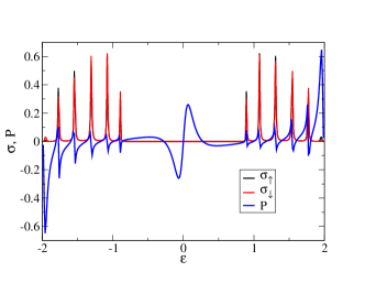
Figure 11: Differential conductances and spin polarization for $\gamma=4$, $10$ unit cells, $\lambda=2,\lambda_{R}=2,B_{x}=0.1$. In this case the Berry phase is not quantized but due to the addition of a constant Rashba spin-orbit coupling, there is a low-energy state that is shifted from zero energy due to the presence of a finite $B_{x}$. The effect of the edge state in the gap is clearly seen in the spin polarization.

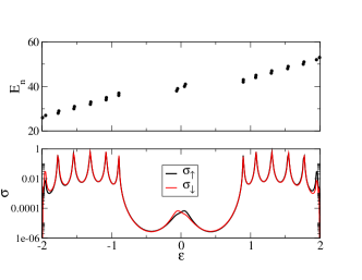
Figure 12: Location of peaks of differential conductance and of eigenenergies of finite system of $10$ unit cells, $E_{n}$, uncoupled to the leads. The parameters used are $\lambda=2,\lambda_{R}=0,B_{x}=0.5,V=0.1$.

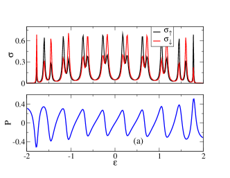
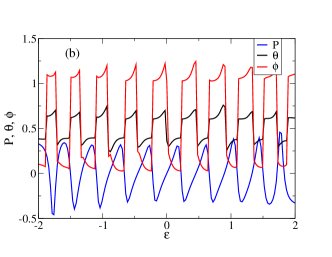
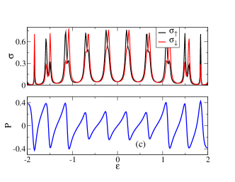
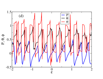
Figure 13: a) and c) Differential conductances and spin polarization and b) and d) angles $\theta$ and $\phi$ of the spin density at the right edge of the chiral chain for topological, (a) and b), and non-topological, c) and d), cases. The parameters are $\gamma=3,\lambda=2,B_{x}=0.5,V=0.5$ and $10$ unit cells for $B_{y}$ given by condition Eq. (19) or $B_{y}=0$.

The charge differential conductances, for incident electrons with spin components $\uparrow,\downarrow$ are obtained as

$$\sigma_{\uparrow} = 1-|r_{\uparrow}|^{2}-|\bar{r}_{\uparrow}|^{2}=|t_{\uparrow}|^{2}+|\bar{t}_{\uparrow}|^{2}$$

$$\sigma_{\downarrow} = 1-|r_{\downarrow}|^{2}-|\bar{r}_{\downarrow}|^{2}=|t_{\downarrow}|^{2}+|\bar{t}_{\downarrow}|^{2}$$ (39)

The spin polarization is defined as

$$P=\frac{\left(|t_{\uparrow}|^{2}+|\bar{t}_{\uparrow}|^{2}\right)-\left(|t_{\downarrow}|^{2}+|\bar{t}_{\downarrow}|^{2}\right)}{\left(|t_{\uparrow}|^{2}+|\bar{t}_{\uparrow}|^{2}\right)+\left(|t_{\downarrow}|^{2}+|\bar{t}_{\downarrow}|^{2}\right)}$$ (40)

The reflection (transmission) coefficients $r_{\sigma}$ ($t_{\sigma}$) of an incident electron with spin $\sigma$ with no spin flip, and the coefficients with spin flip $\bar{r}_{\sigma}$ ($\bar{t}_{\sigma}$) are defined in Appendix B.

VI.2 Results

Applying a magnetic field along the chain direction naturally leads to a spin polarization along that axis. In the following we consider that $B_{z}=0$ and only consider the action of a transverse magnetic field. In Fig. 10 we present results for the spin polarization and the charge diferential conductances, $\sigma_{\uparrow},\sigma_{\downarrow}$ for a chiral chain with $10$ cells with a unit basis of four atoms, $\gamma=4$. As discussed in Appendix B, the effect of any edge states is lost if the chain is large enough, since they decay exponentially towards the interior of the chain. Also, the size of the hopping from the leads to the chiral chain has to be chosen appropriately. We compare the situations when the Berry phase is quantized and when it is trivial. The trivial cases are obtained either adding a Rashba term or considering $B_{y}\neq 0$. In a) and b) two different values of $B_{x}$ are considered. As $B_{x}$ increases from $B_{x}=0.5$ to $B_{x}=1$, the spin polarization increases in magnitude and the gap centered around zero energy also increases. Adding a constant Rashba term in c) increases the gap and comparing b) with d) we see that adding a small $B_{y}=0.2$ does not affect significantly the spin polarization. Note that the various peaks of the spin polarization correlate well with the peaks in the conductances.

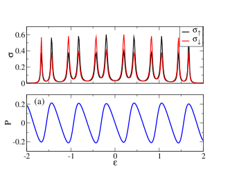
Figure 14: Differential conductances and spin polarization for two sets of parameters that yield an almost periodic spin polarization as the energy changes. The sets of values are for $\gamma=4,V=0.5,B_{x}=B_{y}=0.1$ and a) $10$ cells, $\lambda=2,\lambda_{R}=3,\lambda^{\prime}=3$ and b) $20$ cells, $\lambda=3,\lambda_{R}=4,\lambda^{\prime}=4$.

In Fig. 10(c) a finite Rashba coupling, $\lambda_{R}=2$, is added. This leads, in the finite chiral chain uncoupled to the leads, to the presence of zero energy edge states if $B_{x}=0$, that have a finite energy since $B_{x}\neq 0$. Since $B_{x}$ is large in this case, the state energy is close to the gap and its effect is not seen. In Fig. 11 we consider a smaller value of $B_{x}=0.1$ and its presence is clearly seen in the spin polarization at a small energy inside the gap, of the order of $5\times 10^{-2}$. The contribution of the edge states to the differential conductances is however small, and we need to lower the coupling to the leads, $V$, to see their effect, as shown in Appendix B. In addition to the oscillation in the spin polarization near zero energy, the peaks of the spin polarization correlate well with the peaks of the conductances, as in the previous figure. In Fig. 12 it is shown that the peaks of the differential conductances are located at the eigenenergies of the finite size chiral chain, uncoupled to the leads, with open boundary conditions. Recall that the energy $\epsilon$ considered is not an eigenenergy of the junction and indeed the states are scattering states. Still the resonance with the eigenstates of the uncoupled chain is clearly seen.

The results in Fig. 10 show that the spin polarization is not significantly affected by the Berry phase quantization, even though its effect is felt in the polar angle of the spin density in the chiral chain, both in momentum space and in real space. However, let us analyze the situation in some detail. In Fig. 13 we consider a chain with $\gamma=3$. The quantized Berry phases are found imposing the condition Eq. (19). A simple trivial case is obtained taking $B_{y}=0$. The top panels of Fig. 13 refer to a quantized Berry phase and the lower panels to the trivial case. In Fig. 13(a),(c) we show the differential conductances and the spin polarization and in Fig. 13(b),(d) we show the angles $\theta$ and $\phi$ of the spin density at the right end of the chiral chain. The energies for which $\theta<\pi/2$ ($\theta>\pi/2$) correspond to the regimes where the spin polarization is positive (negative), as expected. Comparing the structure of the conductance peaks we see a similar structure for the quantized and trivial cases (and similar behaviors for the spin polarization) even though it may be argued that in the quantized case the behavior is somewhat more regular. This is emphasized considering the energy dependence of the angles $\theta,\phi$ where a sharper behavior is found in the quantized (topological) case.

A spin polarization that is nearly periodic in the incident energy, may be obtained symmetrizing the spin-orbit coupling (considering equal Rashba, $\lambda_{R}$, and $\lambda^{\prime}$ constant terms, which leads to a gapless spectrum around zero energy) and symmetrizing the transverse external magnetic field (taking $B_{x}=B_{y}\neq 0$). In Fig. 14 we consider two examples that show a rather regular sequence of energy peaks in the differential conductances (and their energy spacings), that lead to a regular set of oscillations and amplitudes of the energy dependent spin polarization. We consider $\gamma=4,V=0.5$ and take $B_{x}=B_{y}=0.1$. Considering a chain with $10$ unit cells the example shown considers $\lambda=2,\lambda_{R}=\lambda^{\prime}=3$ and considering $20$ unit cells we take $\lambda=3,\lambda_{R}=\lambda^{\prime}=4$. We see that increasing the system size the polarization is very nearly periodic.

VII Conclusions

The spinful electronic states of the multiband chiral chain, with a unit cell of size $\gamma$, are the result of the electric field/electric polarization felt by a moving electron that is seen, in the reference frame of the electron, as a modulated spin-orbit coupling. The spectrum is in general gapless.

One way to split the levels is to apply an external magnetic field. Applying a field along $z$ partially lifts the degeneracy and adding a field in the plane transverse to the chain axis, lifts the degeneracies of all bands, giving origin to a gapped system. Turning off $B_{z}$, it is also possible to obtain a gapped system in which the bands are grouped in pairs. One advantage of applying the magnetic field is that it breaks time reversal invariance and allows the possibility of spin transport. Another possible outcome is the possibility of non-trivial topological states as a result of gap openings.

Under appropriate circumstances the gapped system has bands with quantized Berry phases of either individual bands or, in the case of $B_{z}=0$, of pairs of bands. This suggests a topological nature of the bands, in these regimes. The topological character is also revealed by the quantization of the polar angle of the spin density. If the Berry phase is not quantized the polar angle is also not quantized. This is also found diagonalizing the problem in real space, with open boundary conditions, since the polar angle of the spin density averaged over a (bulk) eigenstate of the finite chain is also quantized. We have argued that the quantization of the Berry phase in the case of $\gamma=4$ may be associated with a (hidden) symmetry that is the product of an inversion symmetry and a chiral symmetry, even though these symmetries are absent separately. Edge states are found, displaying very low participation ratio and well localized wave functions on the edges of a finite chain. However, these edge states have finite energies and not zero energy. Moving away from the quantized conditions for the Berry phase and the spin polar angle, we also find edge states. A difference is found that in the quantized Berry phase regime the edge states appear in pairs that are energy degenerate, while in the trivial regime the states are no longer degenerate and either appear as a single state (as for $\gamma=3$) or as consecutive energy states with a finite energy separation (as for $\gamma=4$), at least for the finite sizes considered. Another relevant difference is that if the system size is large enough, the polar angles of the spin density of the edge states are different from each other (between the two degenerate states) and are not quantized.

The gapless chiral model with no external magnetic field may be gapped adding a homogeneous Rashba-like term, revealing the existence of topology and localized zero energy edge states. Adding the external magnetic field to the chiral model with no Rashba-like term, the edge states remain but acquire a finite energy and under appropriate conditions the Berry phase is quantized. Combining the two effects of external magnetic field and Rashba-like term, the model is not topological in the conventional sense, the Berry phase is not quantized, but the edge states remain, both at small and finite energies, and time-reversal symmetry is broken. The breaking of time-reversal symmetry allows a spin polarization in the transport along the chiral chain, and the vicinity to a topological phase leads to the existence of the low energy states in the gap.

We have also considered models where the lattice may be distorted that lead to gap openings in appropriate conditions. For instance, a unit cell with two sites, $\gamma=2$, which may be dimerized, or a unit cell with $\gamma=3$, which may be trimerized in some way. The first case is similar to a SSH model (including spin). The model by itself has a topological regime, with zero energy edge states, quantized winding number and quantized Berry phase. In the case of $\gamma=3$ we showed explicitly that if in addition to the trimerization we add the spin-orbit coupling, even in the absence of an external transverse magnetic field (a field along $z$ is useful to split the bands), a transverse spin density is induced and a quantization of the spin polar angle is found. We also found a quantized Berry phase for a model of electrons with no spin, but with a non-trivial hopping structure, due to the presence of more that one orbital state and considering both nearest neighbor and next-nearest neighbor terms (with a complex part), as shown in Appendix A.

In the case the Berry phase is quantized, the energy dependence of the spin polarization has a better defined structure in comparison to a general case with no Berry phase quantization. Adding a Rashba-like homogeneous spin-orbit term, the contribution of the near zero energy edge states leads to an increase of the low-energy spin polarization. Also, we found a nearly energy periodic structure for the spin polarization considering symmetric homogeneous couplings and a symmetric transverse transverse magnetic field.

As a final note the helix may also be seen as a ladder where one chain has spin up and the other spin down and it may be related to other models. Alternating spin up and spin down the helix is related to a Creutz ladder creutz ; platero : $\gamma=4$ a staggered Creutz ladder with fluxes $0$ and $\pi$. For $\gamma=3$ trimerized ladder with fluxes $0,2\pi/3,2\pi/3,0,-2\pi/3,-2\pi/3,0$.

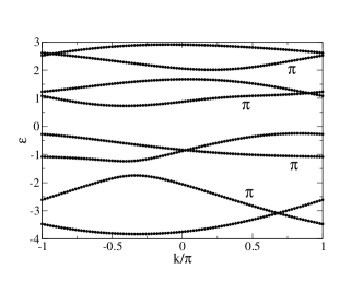
Figure 15: Energy bands and Berry phases of Hamiltonian Eq. (LABEL:Horbital) for $t_{1}=1,t_{2}=0.5,t_{\perp}=1,\Delta(1)=-1,\Delta(2)=1$.

Appendix A Orbital coupling

Another possibility that has been considered is to ignore the spin contribution and to look for an orbital origin liu . In this context, at each molecule in the helix one considers different states associated with the orbital degrees of freedom. The chiral nature of the molecule is implemented introducing a twist (phase) in the hoppings between different orbitals of neighboring molecules. One may understand such a construction considering now that the electron actually moves along the helix and therefore has momentum components along the $xy$ plane. Under the action of the electric field the effective magnetic field has now a $z$-component (along the axis of the helix) that may be seen as a flux that gives origin to an orbital effect (due to the corresponding vector potential) that may be incorporated as a Peierls factor in the effective hoppings between the molecules. To simplify one may just consider that at each molecule two states of orbital nature contribute.

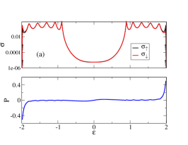
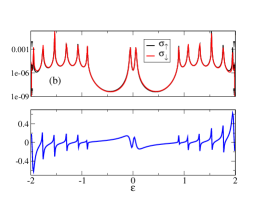
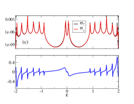
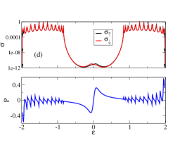
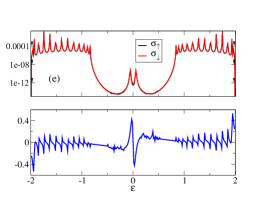
Figure 16: Comparison of different numbers of cells and coupling to the leads, for $\gamma=4$. In the top row the number of cells is $10$ and in the lower row is $20$. We consider $\lambda=2,\lambda_{R}=2,B_{x}=0.1$. We take a) $V=1$, b) $V=0.1$, c) $V=0.05$ d) $V=0.5$, e) $V=0.1$ and f) $V=0.05$.

Here we disregard the spin content of the electrons and consider that at each location there are two states, labeled by $m_{l}=1,2$. The Hamiltonian in real space is chosen as

$$H = \sum_{j}\sum_{m_{l}}\left(-\mu+\Delta(m_{l})\right)c_{j,m_{l}}^{\dagger}c_{j,m_{l}}$$

$$- t_{1}\sum_{j}\sum_{m_{l}}\left(c_{j,m_{l}}^{\dagger}c_{j+1,m_{l}}+c_{j+1,m_{l}}^{\dagger}c_{j,m_{l}}\right)$$

$$- t_{\perp}\sum_{j}\left(c_{j,2}^{\dagger}c_{j,1}+c_{j,1}^{\dagger}c_{j,2}\right)$$

$$- t_{2}\sum_{j}\left(c_{j+1,2}^{\dagger}c_{j,1}+c_{j,1}^{\dagger}c_{j+1,2}\right)$$

$$- t_{2}\sum_{j}\left(e^{-i2\pi/\gamma}c_{j-1,2}^{\dagger}c_{j,1}+e^{i2\pi/\gamma}c_{j,1}^{\dagger}c_{j-1,2}\right)$$

The local hopping between the two orbital states $t_{\perp}$ lifts the degeneracy of the orbital bands, if large enough. Also, we consider $\Delta(1)=-1,\Delta(2)=1$ and $\mu=0$. The action of the orbital chiral coupling, $t_{2}$, is determinant. If the phase of the nearest-neighbor hopping $t_{2}$ vanishes, the bands are gapless. In order to look for topological bands we focus on bands that have gaps. Taking $t_{\perp}=1$ we get a set of bands as shown in Fig. 15. We consider, as an example, $\gamma=4$ and therefore we have eight bands, since $m_{l}=1,2$. The bands are separated by finite gaps. Some of the bands have finite Berry phases of $\gamma_{B}=\pi$.

Appendix B Spin transport

B.1 Transfer matrix and scattering states coefficients

Consider an electron with spin up coming from the left lead, with a given energy $\epsilon$. We choose

$$\left(\begin{array}[]{c}u_{\uparrow}(N_{L})\\ u_{\downarrow}(N_{L})\end{array}\right)=\left(\begin{array}[]{c}1\\ 0\end{array}\right)+r\left(\begin{array}[]{c}1\\ 0\end{array}\right)+\bar{r}\left(\begin{array}[]{c}0\\ 1\end{array}\right)$$ (42)

where $r$ is the reflection coefficient and $\bar{r}$ the reflection coefficient with spin flip, and

$$\left(\begin{array}[]{c}u_{\uparrow}(N_{L}-1)\\ u_{\downarrow}(N_{L}-1)\end{array}\right)=\left(\begin{array}[]{c}1\\ 0\end{array}\right)e^{-iq_{1}}+r\left(\begin{array}[]{c}1\\ 0\end{array}\right)e^{iq_{1}}+\bar{r}\left(\begin{array}[]{c}0\\ 1\end{array}\right)e^{iq_{1}}$$ (43)

where $q_{1}=\cos^{-1}\left(-\epsilon/(2w_{2})\right)$ and $w_{2}$ is the hopping on the left (and right) leads.

Considering an electron with spin down coming from the left lead, with a given energy $\epsilon$, leads to

$$\left(\begin{array}[]{c}u_{\uparrow}(N_{L})\\ u_{\downarrow}(N_{L})\end{array}\right)=\left(\begin{array}[]{c}0\\ 1\end{array}\right)+r\left(\begin{array}[]{c}0\\ 1\end{array}\right)+\bar{r}\left(\begin{array}[]{c}1\\ 0\end{array}\right)$$ (44)

and

$$\left(\begin{array}[]{c}u_{\uparrow}(N_{L}-1)\\ u_{\downarrow}(N_{L}-1)\end{array}\right)=\left(\begin{array}[]{c}0\\ 1\end{array}\right)e^{-iq_{1}}+r\left(\begin{array}[]{c}0\\ 1\end{array}\right)e^{iq_{1}}+\bar{r}\left(\begin{array}[]{c}1\\ 0\end{array}\right)e^{iq_{1}}$$ (45)

On the right lead, we have the transmited wave. In the case of an electron with spin up coming from the left lead, with a given energy $\epsilon$, we have

$$\left(\begin{array}[]{c}u_{\uparrow}(N_{R})\\ u_{\downarrow}(N_{R})\end{array}\right)=t\left(\begin{array}[]{c}1\\ 0\end{array}\right)+\bar{t}\left(\begin{array}[]{c}0\\ 1\end{array}\right)$$ (46)

where $t$ is the transmission coefficient and $\bar{t}$ the transmission coefficient with spin flip, and

$$\left(\begin{array}[]{c}u_{\uparrow}(N_{R}+1)\\ u_{\downarrow}(N_{R}+1)\end{array}\right)=t\left(\begin{array}[]{c}1\\ 0\end{array}\right)e^{iq_{1}}+\bar{t}\left(\begin{array}[]{c}0\\ 1\end{array}\right)e^{iq_{1}}$$ (47)

Considering an electron with spin down coming from the left lead, with a given energy $\epsilon$, leads to

$$\left(\begin{array}[]{c}u_{\uparrow}(N_{R})\\ u_{\downarrow}(N_{R})\end{array}\right)=t\left(\begin{array}[]{c}0\\ 1\end{array}\right)+\bar{t}\left(\begin{array}[]{c}1\\ 0\end{array}\right)$$ (48)

and

$$\left(\begin{array}[]{c}u_{\uparrow}(N_{R}+1)\\ u_{\downarrow}(N_{R}+1)\end{array}\right)=t\left(\begin{array}[]{c}0\\ 1\end{array}\right)e^{iq_{1}}+\bar{t}\left(\begin{array}[]{c}1\\ 0\end{array}\right)e^{iq_{1}}$$ (49)

The normalization (conservation of probability/charge) implies

$$1 = |r_{\uparrow}|^{2}+|\bar{r}_{\uparrow}|^{2}+|t_{\uparrow}|^{2}+|\bar{t}_{\uparrow}|^{2}$$

$$1 = |r_{\downarrow}|^{2}+|\bar{r}_{\downarrow}|^{2}+|t_{\downarrow}|^{2}+|\bar{t}_{\downarrow}|^{2}$$ (50)

Explicitly, the transfer matrix is given by

$$M_{n}=\left(\begin{array}[]{cccc}C&D\\ I&0\end{array}\right)$$ (51)

with

$$C=\left(\begin{array}[]{cc}\frac{-\left(B_{z}+\epsilon\right)w-\left(B_{x}+iB_{y}\right)\lambda\psi_{n}}{w^{2}+\lambda^{2}}&\frac{-\left(B_{x}-iB_{y}\right)w-\left(-B_{z}+\epsilon\right)\lambda\psi_{n}}{w^{2}+\lambda^{2}}\\ \frac{\left(B_{z}+\epsilon\right)\lambda\psi_{n}^{*}-\left(B_{x}+iB_{y}\right)w}{w^{2}+\lambda^{2}}&\frac{\left(B_{x}-iB_{y}\right)\lambda\psi_{n}^{*}-\left(-B_{z}+\epsilon\right)w}{w^{2}+\lambda^{2}}\end{array}\right)$$ (52)

and

$$D=\left(\begin{array}[]{cc}\frac{-w^{2}+\lambda^{2}\psi_{n}\psi_{n-1}^{*}}{w^{2}+\lambda^{2}}&\frac{-w\lambda\psi_{n-1}-w\lambda\psi_{n}}{w^{2}+\lambda^{2}}\\ \frac{w\lambda\psi_{n}^{*}+w\lambda\psi_{n-1}^{*}}{w^{2}+\lambda^{2}}&\frac{-w^{2}+\lambda^{2}\psi_{n}^{*}\psi_{n-1}}{w^{2}+\lambda^{2}}\\ \end{array}\right)$$ (53)

$I$ is the identity and $0$ the null matrix. The coefficients, for a scattering state in a spin up incident electron, may be obtained solving the equations houston

$$A_{\uparrow}\left(\begin{array}[]{c}r\\ t\\ \bar{r}\\ \bar{t}\end{array}\right)=b_{\uparrow}$$ (54)

where

$$b_{\uparrow}=-\left(\begin{array}[]{c}M_{11}^{T}+M_{13}^{T}e^{-iq_{1}}\\ M_{21}^{T}+M_{23}^{T}e^{-iq_{1}}\\ M_{31}^{T}+M_{33}^{T}e^{-iq_{1}}\\ M_{41}^{T}+M_{43}^{T}e^{-iq_{1}}\end{array}\right)$$ (55)

and

$$A_{\uparrow}=\left(\begin{array}[]{cccc}M_{11}^{T}+M_{13}^{T}e^{iq_{1}}&-e^{iq_{1}}&M_{12}^{T}+M_{14}^{T}e^{iq_{1}}&0\\ M_{21}^{T}+M_{23}^{T}e^{iq_{1}}&0&M_{22}^{T}+M_{24}^{T}e^{iq_{1}}&-e^{iq_{1}}\\ M_{31}^{T}+M_{33}^{T}e^{iq_{1}}&-1&M_{32}^{T}+M_{34}^{T}e^{iq_{1}}&0\\ M_{41}^{T}+M_{43}^{T}e^{iq_{1}}&0&M_{42}^{T}+M_{44}^{T}e^{iq_{1}}&-1\\ \end{array}\right)$$ (56)

and similarly for a spin down incident electron.

B.2 Influence of chain size and coupling to leads

As mentioned before, the detection of the edge localized states is enhanced considering relatively small systems, so that the exponential decay of the wave functions is not significative. Also, the smallness of the coupling to the leads is required otherwise the edge states do not give a significant contribution to the differential conductance.

Some examples of the balance of these dependencies is considered in Fig. 16 considering as an example two chains with $10$ and $20$ unit cells and different couplings $V$. As the results show the spin polarization is more sensitive to the edge states, since it is given by a ratio of coefficients as shown in Eq. (40). Intermediate values of the coupling, $V=0.1,0.5$, for the system sizes considered give reasonable results.

References

- (1) T. Yu, Z. Luo and G. E. W. Bauer, arXiv:2206.05535.
- (2) Z. Xie, T.Z. Markus, S. R. Cohen, Z. Vager, R. Gutierrez, and R. Naaman, Nano Lett. 11, 4652 (2011).
- (3) A.- M. Guo, and Q.- F. Sun, Phys. Rev. Lett. 108, 218102 (2012).
- (4) R. Gutierrez, E. Díaz, R. Naaman, and G. Cuniberti, Phys. Rev. B 85, 081404(R) (2012).
- (5) A. A. Eremko and V. M. Loktev, Phys. Rev. B 88, 165409 (2013).
- (6) R. Gutierrez, E. Díaz, C. Gaul, T. Brumme, F. Domínguez-Adame, and G. Cuniberti, J. Phys. Chem. C 117, 22276 (2013).
- (7) R. Gutierrez, and G. Cuniberti, Acta Phys. Polon. A 127, 185 (2015).
- (8) R. Naaman and D. H. Waldeck, Annu. Rev. Phys. Chem. 66, 263 (2015).
- (9) S. Varela, V. Mujica, and E. Medina, Phys. Rev. B 93, 155436 (2016).
- (10) R. A. Caetano, Sci. Reports 6, 23452 (2016).
- (11) S. Matityahu, Y. Utsumi, A. Aharony, O. E.- Wohlman, and C. A. Balseiro, Phys. Rev. B 93, 075407 (2016).
- (12) Yasuhiro Utsumi, Ora Entin-Wohlman, and Amnon Aharony Phys. Rev. B 102, 035445 (2020).
- (13) A. Inui, R. Aoki, Y. Nishiue, K. Shiota, Y. Kousaka, H. Shishido, D. Hirobe, M. Suda, J.-ichiro Ohe, J-ichiro. Kishine, H. M. Yamamoto, and Y. Togawa, Phys. Rev. Lett. 124, 166602 (2020)
- (14) Ferdinand Evers, Amnon Aharony, Nir Bar-Gill, Ora Entin-Wohlman, Per Hedegärd, Oded Hod, Pavel Jelinek, Grzegorz Kamieniarz, Mikhail Lemeshko, Karen Michaeli, Vladimiro Mujica, Ron Naaman, Yossi Paltiel, Sivan Refaely-Abramson, Oren Tal, Jos Thijssen, Michael Thoss, Jan M. van Ruitenbeek, Latha Venkataraman, David H. Waldeck, Binghai Yan, and Leeor Kronik, Adv. Mater. 34, 2106629 (2022), arXiv:2108.09998.
- (15) Y. Liu, J. Xiao, J. Koo, and B. Yan, Nature Materials 20, 638 (2021), arXiv:2008.08881 (2020).
- (16) J. Fransson, Nano Lett. 21, 3026 (2021), arXiv:2103.00840.
- (17) V.L. Lorman and B. Mettout, Phys. Rev. Lett. 82, 940 (1999).
- (18) A. Jákli, O. D. Laventrovich and J. V. Selinger, Rev. Mod. Phys 90, 045004 (2018).
- (19) V.L. Lorman and B. Mettout, Phys. Rev. E 69, 061710 (2004).
- (20) B. Mettout, Phys. Rev. E 75, 011706 (2007).
- (21) W. P. Su, J. R. Schrieffer, and A. J. Heeger, Phys. Rev. Lett. 42, 1698 (1979).
- (22) R. Verresen, N. G. Jones and F. Pollmann, Phys. Rev. Lett. 120, 057001 (2018).
- (23) O. Balabanov, D. Erkensten and H. Johannesson, Phys. Rev. Research 3, 043048 (2021).
- (24) Linhu Li, Zhihao Xu, and Shu Chen, Phys. Rev. B 89, 085111 (2014).
- (25) Zhi-Hai Liu, O. Entin-Wohlman, A. Aharony, J. Q. You, and H. Q. Xu, Phys. Rev. B 104, 085302 (2021).
- (26) A.- M. Guo, and Q.- F. Sun, Phys. Rev. B 95, 155411 (2017).
- (27) Thomas Schuster, Felix Flicker, Ming Li, Svetlana Kotochigova, Joel E. Moore, Jun Ye, and Norman Y. Yao, Phys. Rev. A 103, 063322 (2021).
- (28) J. Zak, Phys. Rev. Lett. 62, 2747 (1989).
- (29) T. P. Pareek and P. Bruno, Phys. Rev. B 65, 241305(R) (2002).
- (30) M. Z. Hasan and C. L. Kane, Rev. Mod. Phys. 82, 3045 (2010).
- (31) X.- L- Qi and S. C. Zhang, Rev. Mod. Phys. 83, 1057 (2011).
- (32) C. L. Kane and E. J. Mele, Phys. Rev. Lett. 95, 146802 (2005); Phys. Rev. Lett. 95, 226801 (2005).
- (33) P. Gentile, M. Cuoco and C. Ortix, Phys. Rev. Lett. 115, 256801 (2015).
- (34) Mariana Malard, David Brandao, Paulo Eduardo de Brito, and Henrik Johannesson, Phys. Rev. Research 2, 033246 (2020).
- (35) A.P. Schnyder, S. Ryu, A. Furusaki and A.W.W. Ludwig, Phys. Rev. B 78, 195125 (2008).
- (36) W. A. Benalcazar, B. A. Bernevig and T. L. Hughes, Phys. Rev. B 96, 245115 (2017).
- (37) D. Xiao, M.-C. Chang and Q. Niu, Rev. Mod. Phys. 82, 1959 (2010).
- (38) R. Resta, J. Phys. Condens. Matter 22, 123201 (2010).
- (39) T. Fukui, Y. Hatsugai and H. Suzuki, J. Phys. Soc. Japan 74, 1674 (2005).
- (40) R. D. King-Smith and D. Vanderbilt, Phys. Rev. B 47, 1651 (1993).
- (41) R. Resta, Rev. Mod. Phys. 66, 899 (1994).
- (42) M. Bahari and M. V. Hosseini, Phys. Rev. B 94, 125119 (2016).
- (43) B. Dong and X.L. Lei, Annals of Phys. 396, 245 (2018).
- (44) Oleksandr Balabanov, and Henrik Johannesson, J. Phys.: Condens. Matter 32, 015503 (2020).
- (45) R. Landauer, Philos. Mag. 21, 863 (1970); D. C. Langreth and E. Abrahams, Phys. Rev. B 24, 2978 (1981); M. Büttiker, Y. Imry, R. Landauer and S. Pinhas, Phys. Rev. B 31, 6207 (1985); M. Büttiker and T.M. Klapwijk, Phys. Rev. B 33, 5114 (1986).
- (46) J.-X. Zhu and C.S. Ting, Phys. Rev. B 61, 1456 (2000).
- (47) M. Creutz, Phys. Rev. Lett. 83, 2636 (1999).
- (48) Juan Zurita, Charles Creffield, and Gloria Platero, Quantum 5, 591 (2021).