Event-Triggered Time-Varying Bayesian Optimization

Abstract

We consider the problem of sequentially optimizing a time-varying objective function using time-varying Bayesian optimization (TVBO). To cope with stale data arising from time variations, current approaches to TVBO require prior knowledge of a constant rate of change. However, in practice, the rate of change is usually unknown. We propose an event-triggered algorithm, ET-GP-UCB, that treats the optimization problem as static until it detects changes in the objective function online and then resets the dataset. This allows the algorithm to adapt to realized temporal changes without the need for prior knowledge. The event-trigger is based on probabilistic uniform error bounds used in Gaussian process regression. We show in numerical experiments that ET-GP-UCB outperforms state-of-the-art algorithms on synthetic and real-world data and provide regret bounds for the proposed algorithm. The results demonstrate that ET-GP-UCB is readily applicable without prior knowledge on the rate of change.

1 Introduction

Over the last two decades, Bayesian optimization (BO) has emerged as a powerful method for sequential decision making and design of experiments under uncertainty (Garnett 2023). These problems are typically formalized as optimization problems of a static unknown objective function. At the core of BO is the exploration-exploitation trade-off, where the decision maker weights the potential benefit of a new unexplored query against the known reward of the currently assumed optimum. The performance of BO algorithms is typically measured in terms of regret, i.e., the difference between the actual decision taken and the (unknown) optimal one. If one assumes a static objective function, there exist algorithms that achieve a desirable sub-linear regret (see Garnett (2023) for an overview), meaning they will efficiently converge to the globally optimal solution.

Figure 1: Illustration of our proposed concept. After the standard BO steps of optimizing the acquisition function and obtaining an observation, an event-trigger decides whether to reset the dataset ($\gamma_{\mathrm{reset}}=1$) or augment it with the observered data point in the usual way ($\gamma_{\mathrm{reset}}=0$). This event-trigger allows our algorithm ET-GP-UCB to be adaptive to changes in the objective function without relying on prior knowledge of the rate of change.

In the real world, however, objective functions are often time-varying. A time-varying objective function alters the nature of the exploration-exploitation trade-off. The optimal decision and the information a decision maker gains from each query are now affected by time and any collected dataset becomes stale. Generally, in a setting of ongoing changes, we cannot expect to find the optimal query and conversely no algorithm can achieve sub-linear regret (Besbes, Gur, and Zeevi 2015, Proposition 1). Instead, our goal is to design algorithms with an explicit relation between regret and the rate of change $\varepsilon$. In their seminal work, Bogunovic, Scarlett, and Cevher (2016) proposed two algorithms for the time-varying Bayesian optimization (TVBO) problem; however, the proposed algorithms and their subsequent variants rely on prior knowledge of the rate of change $\varepsilon$ as a hyperparameter, which can be hard to obtain. Moreover, in these algorithms, $\varepsilon$ is specified at the start and assumed to remain constant over time, which is often not the case in practice.

To address these limitations, we propose the novel concept of event-triggered TVBO (Fig. 1). We model the objective function as time-invariant until an event-trigger detects a significant deviation of the observed data from the current model. The algorithm then reacts to this change by resetting the dataset. This way, the time-varying nature of the problem is only considered in the algorithm’s exploration-exploitation trade-off when necessary. The event-trigger replaces prior knowledge of a rate of change and ET-GP-UCB exhibits good empirical performance for different time variations, including gradual, sudden, and no change as well as desirable theoretical properties under common regularity assumptions. In summary, our contributions are as follows:

1. The novel concept of using an event-trigger in combination with TVBO.

2. An event-triggerd BO algorithm for TVBO called Event-Triggered GP-UCB (ET-GP-UCB) to optimize time-varying objective functions. It does not rely on an estimate of the rate of change and adapts to changes in the objective functions.

3. Empirical evaluations of ET-GP-UCB on synthetic data and real-world benchmarks.

4. Bayesian regret bounds for ET-GP-UCB.

2 Problem Setting

We aim to sequentially optimize an unknown time-varying objective function $f_{t}\colon\mathbb{X}\to\mathbb{R}$ on a compact set $\mathbb{X}\subset\mathbb{R}^{d}$ as

$$\bm{x}_{t}^{*}=\arg\max_{\bm{x}\in\mathbb{X}}f_{t}(\bm{x})$$ (1)

over the discrete time steps $t\in\mathbb{I}_{1:T}$ up to the time horizon $T$. At each time step, an algorithm chooses a query $\bm{x}_{t}\in\mathbb{X}$ and obtains noisy observations following the standard assumption in BO.

Assumption 1.

Observations $y_{t}=f_{t}(\bm{x}_{t})+w_{t}$ are perturbed by independent and identically distributed (i.i.d.) Gaussian noise with noise variance $\sigma_{n}^{2}$ as $w_{t}\sim\mathcal{N}(0,\sigma_{n}^{2})$.

Without assumptions on the temporal change, the problem is intractable. Thus, we impose a Markov chain model proposed by Bogunovic, Scarlett, and Cevher (2016) and used in various applications (Su et al. 2018; König et al. 2021).

Assumption 2 (Bogunovic, Scarlett, and Cevher (2016)).

Let $\mathcal{GP}\left(\mu,k(\bm{x},\bm{x}^{\prime})\right)$ be a Gaussian process (GP) with mean function $\mu:\mathbb{X}\to\mathbb{R}$ and kernel $k\colon\mathbb{X}\times\mathbb{X}\to\mathbb{R}$. Given i.i.d. samples $g_{1},g_{2},\dots$ with $g_{i}\sim\mathcal{GP}\left(0,k(\bm{x},\bm{x}^{\prime})\right)$, where $k(\bm{x},\bm{x}^{\prime})$ is a stationary kernel with $k(\bm{x},\bm{x}^{\prime})\leq 1$ for all $\bm{x},\bm{x}^{\prime}\in\mathbb{R}$, and a rate of change $\varepsilon\in[0,1]$, the time-varying objective function $f_{t}(\bm{x})$ follows the Markov chain:

$$f_{t}(\bm{x})=\begin{cases}g_{t}(\bm{x})\,,&t=1\\ \sqrt{1-\varepsilon}f_{t-1}(\bm{x})+\sqrt{\varepsilon}g_{t}(\bm{x})\,,&t\geq 2.\end{cases}$$ (2)

Remark.

Due to Assumption 2, any choice of $\varepsilon\in[0,1]$ yields that $f_{t}\sim\mathcal{GP}\left(0,k\right)$ for all $t\in\mathbb{I}_{1:T}$.

We further use standard smoothness assumptions on the kernel choice introduced in Srinivas et al. (2010) as well as Bogunovic, Scarlett, and Cevher (2016).

Assumption 3 (Bogunovic, Scarlett, and Cevher (2016)).

The kernel $k(\bm{x},\bm{x}^{\prime})$ is such that, given $f\sim\mathcal{GP}\left(0,k(\bm{x},\bm{x}^{\prime})\right)$, $L,L_{f}\geq 1$, and $a_{0},b_{0},a_{1},b_{1}\geq 0$, the following holds:

$$\mathbb{P}\left\{\sup_{\bm{x}\in\mathbb{X}}\left\lvert f\right\rvert>L_{f}\right\} \leq a_{0}e^{-\left(L_{f}/b_{0}\right)^{2}}\,\text{and}$$ (3)

$$\mathbb{P}\left\{\sup_{\bm{x}\in\mathbb{X}}\left\lvert\partial f/\partial x_{j}\right\rvert>L\right\} \leq a_{1}e^{-\left(L/b_{1}\right)^{2}},j=1,...,d.$$ (4)

This assumption limits the choice of kernel to those that are at least four times differentiable (Ghosal and Roy 2006, Theorem 5), such as a squared exponential kernel.

The performance of an algorithm optimizing (1) is measured in terms of the cumulative regret $R_{T}$.

Definition 1 (Regret).

Let $\bm{x}_{t}^{*}$ be the maximizer of $f_{t}(\bm{x})$, and let $\bm{x}_{t}\in\mathbb{X}$ be the query at time step $t$. Then, the instantaneous regret at $t$ is $r_{t}=f_{t}(\bm{x}_{t}^{*})-f_{t}(\bm{x}_{t})$, and the regret after $T$ time steps is $R_{T}=\sum_{t=1}^{T}r_{t}$.

Sub-linear regret is defined as $\lim_{T\to\infty}R_{T}/T=0$. In the time-invariant setting ($\varepsilon=0$), algorithms can achieve such sub-linear regret, e.g., GP-UCB (Srinivas et al. 2010, Theorem 2) with regret of order $\tilde{\mathcal{O}}(\sqrt{T})$. For a time-varying objective function following Assumption 2, Bogunovic, Scarlett, and Cevher (2016, Theorem 4.1) shows that the best possible expected regret of an algorithm is linear as $\tilde{\mathcal{O}}(T\varepsilon)$.

Problem Statement: We consider the time-varying optimization problem (1) under Assumptions 1–3. To develop a practical algorithm, and in contrast to the state-of-the-art in TVBO, we assume the rate of change $\varepsilon$ to be unknown. From the theoretic point of view, the algorithm should obtain regret bounds that are no more than linear in $T$ and explicitly dependent on the true $\varepsilon$.

3 Related Work and Background

Our work builds on prior work in BO and TVBO. This section gives an overview of related work in these two fields.

Bayesian Optimization

Our event-trigger design and algorithm extends prior work by Srinivas et al. (2010) on the BO algorithm GP-UCB and transfers some of their concepts to the time-varying setting. Srinivas et al. (2010) proved sub-linear regret bounds when using an upper confidence bound (UCB) acquisition function of the form $\mu_{\mathcal{D}_{t}}(\bm{x})+\sqrt{\beta}_{t}\sigma_{\mathcal{D}_{t}}(\bm{x})$, with standard posterior updates of the GP model, given a dataset $\mathcal{D}_{t}\coloneqq\left\{(\bm{x}_{i},y_{i})\right\}_{i=1}^{t-1}$, as

$$\mu_{\mathcal{D}_{t}}(\bm{x}) =\bm{k}_{t}(\bm{x})^{T}\left(\textbf{K}_{t}+\sigma_{n}^{2}\textbf{I}\right)^{-1}\bm{y}_{t}$$ (5)

$$\sigma_{\mathcal{D}_{t}}^{2}(\bm{x}) =k(\bm{x},\bm{x})-\bm{k}_{t}(\bm{x})^{T}\left(\textbf{K}_{t}+\sigma_{n}^{2}\textbf{I}\right)^{-1}\bm{k}_{t}(\bm{x})$$ (6)

where $\textbf{K}_{t}=[k(\bm{x}_{i},\bm{x}_{j})]_{i,j=1}^{t-1}$ is the Gram matrix, $\bm{k}_{t}(\bm{x})=[k(\bm{x}_{i},\bm{x})]_{i=1}^{t-1}$, and noisy measurements $\bm{y}_{t}=[y_{1},\dots,y_{t-1}]^{T}$ follow Assumption 1. Our algorithm uses these standard posterior updates only as long as all the measurements are still compliant with the current posterior model; it resets the dataset if this is no longer the case. Consequently, in contrast to GP-UCB, our algorithm can adapt to changes in the objective function by discarding stale data.

In the regret bounds of Srinivas et al. (2010), the mutual information gain $I(\bm{f}_{M},\bm{y}_{M})=\frac{1}{2}\ln\det(\textbf{I}+\sigma_{n}^{2}\textbf{K}_{M})$ over $M$ points with $\bm{f}_{M}=[f_{1}(\bm{x}_{1}),\dots,f_{M}(\bm{x}_{M})]$ takes an important role. The maximum information gain one can obtain using a time-invariant GP model over any set of points is $\gamma_{M}\coloneqq\max_{\bm{x}_{1},\dots,\bm{x}_{M}}I(\bm{f}_{M},\bm{y}_{M}).$ Like Srinivas et al. (2010), we will leverage this in our theoretical analysis of ET-GP-UCB. For a detailed analysis of other BO algorithms, we refer to Garnett (2023).

Time-Varying Bayesian Optimization

TVBO can be considered a special case of contextual BO (Krause and Ong 2011), with the key distinction that time is strictly increasing; therefore, it is not possible to choose samples in the whole context domain. TVBO was first explicitly discussed by Bogunovic, Scarlett, and Cevher (2016), where they presented two time-varying UCB variants. They propose that changes in the objective function can be modeled as in Assumption 2. The corresponding GP surrogate model explicitly models these time variations in (5) and (6) as

$$\tilde{\mu}_{\mathcal{D}_{t}}(\bm{x}) =\tilde{\bm{k}}_{t}(\bm{x})^{T}\left(\tilde{\textbf{K}}_{t}+\sigma_{n}^{2}\textbf{I}\right)^{-1}\bm{y}_{t}$$ (7)

$$\tilde{\sigma}_{\mathcal{D}_{t}}^{2}(\bm{x}) =k(\bm{x},\bm{x})-\tilde{\bm{k}}_{t}(\bm{x})^{T}\left(\tilde{\textbf{K}}_{t}+\sigma_{n}^{2}\textbf{I}\right)^{-1}\tilde{\bm{k}}_{t}(\bm{x})$$ (8)

where $\tilde{\textbf{K}}_{t}=\textbf{K}_{t}\circ\textbf{K}^{\text{time}}_{t}$ with $\textbf{K}^{\text{time}}_{t}=[(1-\varepsilon)^{|i-j|/2}]_{i,j=1}^{t-1}$, and $\tilde{\bm{k}}_{t}(\bm{x})=\bm{k}_{t}(\bm{x})\circ\bm{k}^{\text{time}}_{t}$ with $\bm{k}^{\text{time}}_{t}=[(1-\varepsilon)^{|t+1-i|/2}]_{i=1}^{t-1}$, and $\circ$ is the Hadamard product. These updates ensure that the posterior distribution follows the same dynamics as $f_{t}$ (cf. Assumption 2). We will utilize this in our proof of Bayesian regret bounds for ET-GP-UCB.

Since the introduction of this setting in the seminal paper by Bogunovic, Scarlett, and Cevher (2016), their algorithm TV-GP-UCB with posterior updates as in (7) and (8) has been used in various applications, such as controller learning (Su et al. 2018), safe adaptive control (König et al. 2021), and hyperparameter optimization for reinforcement learning (Parker-Holder, Nguyen, and Roberts 2020; Parker-Holder et al. 2021). However, it relies on a priori estimation of the rate of change $\varepsilon$ and assumes $\varepsilon$ stays constant over time. In contrast, the event-trigger in ET-GP-UCB does not need an estimate of the rate of change and enables our algorithm to adapt to changes in the objective function, i.e., it can cope with a time-varying $\varepsilon$ as well as sudden changes. We note that, if the rate of change is known beforehand and the structural assumptions are satisfied, then the TV-GP-UCB model is an efficient choice since these properties are explicitly embedded into the algorithm.

Bogunovic, Scarlett, and Cevher (2016) also introduced R-GP-UCB, which resets the posterior periodically to account for data becoming uninformative over time. In contrast, ET-GP-UCB resets the posterior only if an obtained measurement is no longer consistent with the current dataset (cf. Sec. 4). As in R-GP-UCB, our algorithm uses time-invariant posterior updates within time intervals, but our time intervals do not have to be specified a priori based on $\varepsilon$; rather, they are determined online by the event-trigger.

Under frequentist regularity assumption, Zhou and Shroff (2021) also propose an algorithm with a constant reset time, BR-GP-UCB, as well as a sliding window algorithm SW-GP-UCB. The crucial difference to our problem setting is their assumption of a fixed variational budget, i.e., $\sum_{t=1}^{T}||f_{t+1}-f_{t}||_{\mathcal{H}}<B_{T}$, where $\mathcal{H}$ is a Reproducing Kernel Hilbert Space (RKHS) and $B_{T}$ a scalar. Clearly, the above assumption means that the change in the objective function will converge to zero as $T\rightarrow\infty$. Leveraging these same assumptions, Deng et al. (2022) propose an algorithm, W-GP-UCB, which utilizes a similar weighted GP model to TV-GP-UCB. In this more restrictive setting of a fixed variational budget, sub-linear regret is possible (Besbes, Gur, and Zeevi 2015). In contrast, we are interested in the setting given by Assumption 2, which corresponds to a variational budget that increases linearly in time; hence, the best possible regret is also linear (Besbes, Gur, and Zeevi 2015, Proposition 1). Nevertheless, in Appendix A, we empirically compare ET-GP-UCB against the algorithms of Zhou and Shroff (2021) and Deng et al. (2022) and display improved performance on their benchmarks.

Event-Triggered Learning

The idea of resetting a dataset only if an important change occurs as detected by a trigger event is similar to the concepts of event-triggered learning (Solowjow and Trimpe 2020) and event-triggered online learning (Umlauft and Hirche 2019). In the multi-armed bandit setting (Wei and Luo 2021) discuss the idea of including tests into optimization algorithms to detect and adapt to non-stationarity. All concepts aim to be efficient with the available data, only updating a model when necessary or only adding new data which is relevant. Our approach also aims for data efficiency; as long as we have a good model of our objective function, we want to use already-available data to minimize regret. However, if the event-trigger detects a significant model mismatch, we reset the dataset and thereby delete stale data. While the mentioned approaches consider different problem settings, this one is the first to introduce event-triggers to TVBO.

4 Event-Trigger Design for TVBO

In this section, we design the event-trigger that is at the heart of ET-GP-UCB in Fig. 1 and allows us to adapt to changes when necessary. In essence, we build on state-of-the-art uniform error bounds for GP regression to decide if new data is consistent with the posterior. When new data deviates significantly, we reset the dataset and thus forget old data. While conceptually straightforward, this idea constitutes a new approach compared to previous work in TVBO, as the resulting algorithm does not rely on the rate of change as a hyperparameter. First, we introduce the core component of our general event-triggered TVBO framework, the event-trigger:

Definition 2 (Event-trigger in TVBO).

Given a test function $\psi_{t}$ and a threshold function $\kappa_{t}$, both of which can depend on the current dataset $\mathcal{D}_{t}$ and the latest query location and measurement pair $(\bm{x}_{t},y_{t})$, the event-trigger at time $t$ is

$$\gamma_{\mathrm{reset}}=1\Leftrightarrow\psi_{t}\left(\mathcal{D}_{t},(\bm{x}_{t},y_{t})\right)>\kappa_{t}\left(\mathcal{D}_{t},(\bm{x}_{t},y_{t})\right)$$ (9)

where $\gamma_{\mathrm{reset}}$ is the binary indicator for whether to reset the dataset $(\gamma_{\mathrm{reset}}=1)$ or not $(\gamma_{\mathrm{reset}}=0)$.

We base our event-trigger on uniform error bounds used in GP regression, specifically on the Bayesian error bound by Srinivas et al. (2010, Lemma 5.5). Other design options would also be possible, e.g., likelihood-based event-triggers. In the following, we will denote ${t^{\prime}}\in\mathbb{N}$ as the time since the previous reset. We have ${t^{\prime}}=t$ if no reset has yet occurred.

Lemma 1 (Srinivas et al. (2010, Lemma 5.5)).

Pick $\delta\in(0,1)$ and set $\rho_{{t^{\prime}}}=2\ln{\frac{\pi_{{t^{\prime}}}}{\delta}}$, where $\sum_{{t^{\prime}}\geq 1}\pi_{{t^{\prime}}}^{-1}=1$, $\pi_{{t^{\prime}}}>0$. Let $f\sim\mathcal{GP}(0,k(\bm{x},\bm{x}^{\prime}))$. Then, $|f(\bm{x}_{t})-\mu_{\mathcal{D}_{t}}(\bm{x}_{t})|\leq\sqrt{\rho_{{t^{\prime}}}}\sigma_{\mathcal{D}_{t}}(\bm{x}_{t})$ holds for all ${{t^{\prime}}}\geq 1$ with prob. at least $1-\delta$.

Remark.

For $\sum_{{t^{\prime}}\geq 1}\pi_{{t^{\prime}}}^{-1}=1$ to hold, one can choose $\pi_{{t^{\prime}}}=\pi^{2}{t^{\prime}}^{2}/6$ as in Srinivas et al. (2010).

The result gives a high probability bound for all time steps on the absolute deviation between the posterior mean and a time-invariant objective function at the query location $\bm{x}_{t}$ based on the posterior variance and parameter $\rho_{{t^{\prime}}}$. If a time-varying objective function satisfies this bound for all time steps, the time variations are negligible with high probability (i.e., $\varepsilon\approx 0$). On the other hand, if the bound in Lemma 1 is violated at a chosen query location $\bm{x}_{t}$, the objective function has likely changed. The event-trigger uses these bounds to detect significant changes and resets the stale dataset.

The algorithm needs to evaluate the trigger event at every time step. While it cannot directly evaluate $\left\lvert f_{t}(\bm{x}_{t})-\mu_{\mathcal{D}_{t}}(\bm{x}_{t})\right\rvert$ in Lemma 1 (cf. Assumption 1), we can evaluate $\left\lvert y_{t}-\mu_{\mathcal{D}_{t}}(\bm{x}_{t})\right\rvert$. Thus, we adapt Lemma 1 to design a probabilistic bound which includes only $y_{t}$ instead of $f_{t}(\bm{x}_{t})$. For this, we first bound the noise in probability. All proofs of the following Lemmas are in Appendix C.

Lemma 2.

Pick $\delta\in(0,1)$ and set $\bar{w}_{{t^{\prime}}}^{2}={2\sigma_{n}^{2}\ln\frac{\pi_{{t^{\prime}}}}{\delta}}$, where $\sum_{{{t^{\prime}}}\geq 1}\pi_{{t^{\prime}}}^{-1}=1$, $\pi_{{t^{\prime}}}>0$. Then, the Noise sequence in Assumption 1, obtained since the previous reset, satisfies ${|w_{{t^{\prime}}}|\leq\bar{w}_{{t^{\prime}}}}$ for all ${{t^{\prime}}}\geq 1$ with prob. at least $1-\delta$.

With Lemma 2, we can use Lemma 1 to build a probabilistic error bound that can act as the test function and the corresponding threshold functions of our event-trigger.

Lemma 3.

Let $f_{t}(\bm{x})$ follow Assumption 2 with $\varepsilon=0$. Pick $\delta_{\mathrm{B}}\in(0,1)$ and set $\rho_{{t^{\prime}}}=2\ln{\frac{2\pi_{{t^{\prime}}}}{\delta_{\mathrm{B}}}}$, where $\sum_{{{t^{\prime}}}\geq 1}\pi_{{t^{\prime}}}^{-1}=1$, $\pi_{{t^{\prime}}}>0$. Also set $\bar{w}_{{t^{\prime}}}^{2}={2\sigma_{n}^{2}\ln\frac{2\pi_{{t^{\prime}}}}{\delta_{\mathrm{B}}}}$. Then, observations $y_{t}$ under Assumption 1 satisfy $|y_{t}-\mu_{\mathcal{D}_{t}}(\bm{x}_{t})|\leq\sqrt{\rho_{{t^{\prime}}}}\sigma_{\mathcal{D}_{t}}(\bm{x}_{t})+\bar{w}_{{t^{\prime}}}$ for all ${t^{\prime}}\geq 1$ with prob. at least $1-\delta_{\mathrm{B}}$.

We now define the event-trigger for ET-GP-UCB following Def. 2. As the test and threshold function, we choose

$$\psi_{t}(\bm{x}_{t}) \coloneqq\psi_{t}\left(\mathcal{D}_{t},(\bm{x}_{t},y_{t})\right)=\left\lvert y_{t}-\mu_{\mathcal{D}_{t}}(\bm{x}_{t})\right\rvert$$ (10)

$$\kappa_{t}(\bm{x}_{t}) \coloneqq\kappa_{t}\left(\mathcal{D}_{t},(\bm{x}_{t},y_{t})\right)=\sqrt{\rho_{{t^{\prime}}}}\sigma_{\mathcal{D}_{t}}(\bm{x}_{t})+\bar{w}_{{t^{\prime}}},$$ (11)

respectively, as specified in Lemma 3. With this, we designed a principled event-trigger to detect changes in the objective function. The resulting algorithm ET-GP-UCB is then as follows: We perform standard GP-UCB as long as the event-trigger evaluates to $\gamma_{\mathrm{reset}}=0$. When the event-trigger is activated the objective function $f_{t}$ has likely changed, and the dataset has become stale. ET-GP-UCB then resets the dataset and restarts the optimization. This is summarized in Algorithm 1. The single design parameter of our event-trigger is $\delta_{\mathrm{B}}$ in Lemma 3, which has a well-understood meaning as defining the tightness of the probabilistic uniform error bound. Consequently, we do not need any a priori knowledge of the rate of change $\varepsilon$.

Algorithm 1 Event-triggered GP-UCB (ET-GP-UCB).

1:Define: $\mathcal{GP}(0,k)$, $\mathbb{X}\subset\mathbb{R}^{d}$, $\delta_{\mathrm{B}}\in(0,1)$, $\mathcal{D}_{1}=\emptyset$

2:for $t=1,2,\dots,T$ do

3:     Train GP model with $\mathcal{D}_{t}$

4:     Choose $\beta_{t}$ (e.g., according to Theorem 1, Sec. 6)

5:     Choose $\bm{x}_{t}=\arg\max_{\bm{x}\in\mathbb{X}}\mu_{\mathcal{D}_{t}}(\bm{x})+\sqrt{\beta_{t}}\sigma_{\mathcal{D}_{t}}(\bm{x})$

6:     Sample $y_{t}=f_{t}(\bm{x}_{t})+w_{t}$

7:     $\gamma_{\mathrm{reset}}\leftarrow$ Trigger($\mathcal{D}_{t}$, $(y_{t},\bm{x}_{t}),\delta_{\mathrm{B}}$) $\triangleright$ see (10), (11)

8:     if $\gamma_{\mathrm{reset}}$ then

9:         Reset dataset $\mathcal{D}_{t+1}=\{(y_{t},\bm{x}_{t})\}$

10:     else

11:         Update dataset $\mathcal{D}_{t+1}=\mathcal{D}_{t}\cup\{(y_{t},\bm{x}_{t})\}$      

Our event-trigger can only detect changes in the objective function at the current query location. Even with the local evaluation and the fact that we do not know the rate of change a priori ET-GP-UCB performs well in the theoretic setting of Assumption 2; and, maybe more importantly, it outperforms other algorithms in real-world settings which we demonstrate in the next section. Afterwards, we show regret bounds for ET-GP-UCB in Sec. 6.

5 Empirical Evaluation

Using both synthetic data and standard BO benchmarks, we compare ET-GP-UCB to the state-of-the-art algorithms R-GP-UCB, which resets periodically, and TV-GP-UCB, which gradually forgets past data points. We further compare these time-varying algorithms to the time-invariant GP-UCB as a baseline. In our experiments, we find that:

1. The adaptive resetting of ET-GP-UCB always outperforms periodic resetting.

2. ET-GP-UCB outperforms TV-GP-UCB on synthetic data if the rate of change is misspecified.

3. ET-GP-UCB outperforms periodic resetting and TV-GP-UCB on real-world data.

We reiterate that ET-GP-UCB does not rely on any information regarding the rate of change. To highlight the generalization capabilities of ET-GP-UCB to different scenarios, we use the same parameter for the event-trigger ($\delta_{\mathrm{B}}=0.1$) in all experiments. A sensitivity analysis of the hyperparameter $\delta_{\mathrm{B}}$ on the regret is in Appendix B and shows that ET-GP-UCB performs similar for a wide range of $\delta_{\mathrm{B}}$.

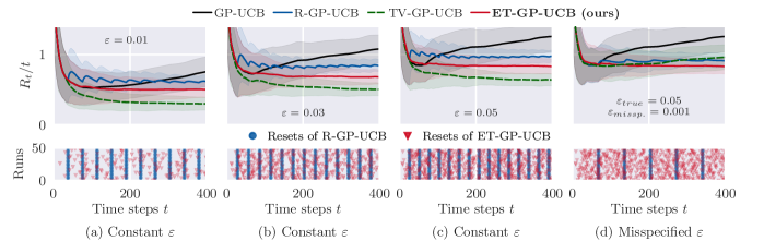
Figure 2: Within-model comparisons. Top row: performance of the different algorithms in terms of normalized regret. The shaded areas show one standard deviation of the respective algorithms. Bottom row: reset timings of R-GP-UCB and ET-GP-UCB. In (a) to (c), $\varepsilon$ is fixed for all time steps, and in (d), $\varepsilon$ is misspecified for TV-GP-UCB and R-GP-UCB. In (a) to (c), TV-GP-UCB is the full information reference, showing the best possible UCB performance with known constant $\varepsilon$. We compare ET-GP-UCB to R-GP-UCB, the latter of which uses the true $\varepsilon$ to determine its periodic reset time. For ET-GP-UCB, we use the same parameter $\delta_{\mathrm{B}}$ in the event-trigger for the test cases (a) to (d). In all cases, ET-GP-UCB outperforms R-GP-UCB. It also outperforms TV-GP-UCB if $\varepsilon$ is misspecified, as shown in (d), since ET-GP-UCB does not rely on prior information on $\varepsilon$.

As in Bogunovic, Scarlett, and Cevher (2016), and similarly to Srinivas et al. (2010), we utilize a logarithmic scaling $\beta_{t}$ as $\beta_{t}=\mathcal{O}(d\ln(t))$, where $\beta_{t}=c_{1}\ln(c_{2}t)$. This approximates $\beta_{t}$ in Theorem 1 (cf. Sec. 6) and allows for a direct comparison to Bogunovic, Scarlett, and Cevher (2016), as they suggest to set $c_{1}=0.8$ and $c_{2}=4$ for a suitable exploration-exploitation trade off. All experiments in this section are conducted using BoTorch (Balandat et al. 2020) and GPyTorch (Gardner et al. 2018).

Within-Model Comparison

First, we consider the same two-dimensional setting for synthetic data as in Bogunovic, Scarlett, and Cevher (2016). We choose the compact set to be $\mathbb{X}=[0,1]^{2}$ and generate $50$ different objective functions according to Assumption 2 with a known $\varepsilon$, a squared exponential kernel with fixed lengthscales $l=0.2$, and a noise variance of $\sigma_{n}^{2}=0.05$. The setting in which all the hyperparameters are known to the algorithm is referred to as within-model comparison (Hennig and Schuler 2012); such comparisons are used to evaluate an algorithm’s performance given all assumptions are fulfilled. Here, TV-GP-UCB acts as the reference case with full information. It shows the best performance an UCB algorithm can obtain in this setting as it takes Assumption 2 explicitly into account by using the time-varying posterior updates in (7) and (8). R-GP-UCB is also parameterized using the true $\varepsilon$ for the periodic reset time as $N_{\text{const}}=\lceil\min\{T,12\varepsilon^{-1/4}\}\rceil$ (Bogunovic, Scarlett, and Cevher 2016, Proposition 4.1). In contrast, ET-GP-UCB does not depend on $\varepsilon$.

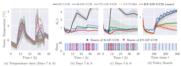
Figure 3: Real-world examples. Subfigure (a) shows the temperature data consisting of sensor measurements from the two test days used in Bogunovic, Scarlett, and Cevher (2016). In (b), the performance of the algorithms on these two days (top) and the resets of R-GP-UCB and ET-GP-UCB (bottom) are displayed. Here, ET-GP-UCB outperforms TV-GP-UCB as well as R-GP-UCB and GP-UCB. Subfigure (c) shows the performance on other test days. Also for these days, ET-GP-UCB shows a performance improvement compared to all other algorithms. For these experiments on real-world data, we use the same parameter for the event-trigger as in all previous experiments whereas TV-GP-UCB and R-GP-UCB relied on estimating $\varepsilon$. Lastly, in subfigure (d), ET-GP-UCB also outperforms all competing baselines on a policy search benchmark.

In the top figures of Fig. 2 (a) to (c), we show the normalized regret for different ${\varepsilon}$. In all cases, ET-GP-UCB outperforms R-GP-UCB without relying on prior knowledge on the rate of change. The bottom figures of Fig. 2 (a) to (c) highlight the adaptive nature of ET-GP-UCB, as the resets do not always occur at the same time, but depend on the realized change in the objective function. This becomes even more apparent looking at Fig. 2 (d), where the rate of change for TV-GP-UCB and R-GP-UCB is misspecified. ET-GP-UCB does not rely on specifying a rate of change a-priori and we do not change any parameters for this experiment. We observe that ET-GP-UCB reacts to the realized changes resulting in the same performance as in Fig. 2 (c). With this, it outperforms TV-GP-UCB and R-GP-UCB which slowly diverge shown by the increase in normalized regret over time.

Real-World Temperature Data

To benchmark the algorithms on real-world data, we use the temperature dataset collected from $46$ sensors deployed at Intel Research Berkeley over eight days at $10$ minute intervals. This dataset was also used as a benchmark in previous work on GP-UCB and TVBO (Srinivas et al. 2010; Krause and Ong 2011; Bogunovic, Scarlett, and Cevher 2016). The objective is to activate the sensor with the highest temperature at each time step resulting in a spatio-temporal monitoring problem. In our TVBO setting, $f_{t}$ consists of all sensor readings at time step $t$, and an algorithm can query only a single sensor every $10$ minutes. Hence, the regret following Def. 1 is the difference between the maximum temperature and the recorded temperature by the activated sensor.

For each experiment, two test days are selected, while the preceding days serve as the training set. Using this training set, all data is normalized to have a mean of zero and a standard deviation of one. The empirical covariance matrix is computed based on the training set and employed as the kernel for all algorithms. The sensor data of the days 7 and 8 is shown in Fig. 3 (a) and an overview of the remaining days is given in Appendix F. For TV-GP-UCB, we set $\varepsilon=0.03$ and the periodic reset time of R-GP-UCB to $N_{\text{const}}=15$ according to Bogunovic, Scarlett, and Cevher (2016). For ET-GP-UCB, we use the same parameter for the event-trigger as in all the previous experiments.

Fig. 3 (b) presents the normalized regret (top) for each algorithm over $20$ runs and the resets of R-GP-UCB and ET-GP-UCB (bottom). Consistent with the experiments on synthetic data, we observe that adaptive resetting outperforms periodic resetting. Furthermore, ET-GP-UCB outperforms TV-GP-UCB. It highlights that using a constant rate of change in the GP model as in TV-GP-UCB can be problematic for real-world problems. Here, being adaptive to changes as ET-GP-UCB is beneficial and yields lower regret. ET-GP-UCB also outperforms the competing algorithms on test days other than the ones used in Bogunovic, Scarlett, and Cevher (2016), as shown in Fig. 3 (c). Considering the resets of ET-GP-UCB, it appears that especially when changes in the objective function are more distinct (e.g., changes between night and day), the proposed event-trigger framework is empirically beneficial compared to using an estimated constant rate of change.

Policy Search in Time-Varying Environments

To further investigate this claim, we compared all algorithms on a four-dimensional policy search benchmark of a cart-pole system also used in Brunzema, von Rohr, and Trimpe (2022). The objective function in this example is quadratic in the optimization variables. Given the system dynamics of the cart-pole system, it is possible to calculate the optimal policy and thus calculate the regret following Def. 1. To induce a sudden change in the objective function, we increase the friction in the bearing at $t=100$ by a factor of $2.5$. We expect the event-trigger of ET-GP-UCB to detect this change in the objective function and converge to the new optimum after resetting the dataset and thus outperform the algorithms based on the assumption of a constant rate of change. In contrast to previous examples, we also perform online hyperparameter optimization of the spatial lengthscales using Gamma priors to guide the search (all parameters are listed in Appendix G). For TV-GP-UCB, we choose $\varepsilon=0.03$ and we pick the constant reset timing of R-GP-UCB according to Bogunovic, Scarlett, and Cevher (2016, Corollary 4.1). In this example, we also compare ET-GP-UCB against UI-TVBO (Brunzema, von Rohr, and Trimpe 2022) as it was specifically designed for policy search in changing environments. For ET-GP-UCB, we again choose the same parameter as in all previous examples. The results over $20$ independent runs are displayed in Fig. 3 (d).

We can observe that ET-GP-UCB is the best performing algorithm since it can detect the change in the objective function and converge to the new optimal solution. We can further see that TV-GP-UCB and R-GP-UCB, which rely on an ongoing and smooth change in the objective function, empirically struggle to cope with such sudden changes resulting in significantly increased regret. While UI-TVBO can also recover from the change, ET-GP-UCB still outperforms this baseline. The example also highlights that a constant reset time that is too short can yield divergent behavior.

6 Theoretical Analysis

In the previous section, we demonstrated the efficacy of our proposed algorithm ET-GP-UCB including its superior performance in real-world settings with various types of changes. We now provide a theoretical analysis of our method ET-GP-UCB including Bayesian regret bounds for the regularity assumptions in Sec. 2. For this, we first define the time at which a reset occurs.

Definition 3.

The random variable corresponding to the activation time of the event-trigger following Def. 2 is denoted by $\tau\coloneqq\min\{t\in\mathbb{N}:\psi_{t}(\bm{x}_{t})>\kappa_{t}(\bm{x}_{t})\}$.

The random variable $\tau$ is a stopping time, as $\psi_{t}(\bm{x}_{t})$ is a discrete-time stochastic process and the trigger-event is completely determined by the information known up to $t$. The stochastic process depends recursively on the acquisition function, which makes an analytical study of the stopping time difficult; even for simple stochastic processes, calculating expected values of stopping times is typically intractable. However, since we know that $\tau$ is a non-negative random variable naturally bounded by the time horizon $T$, we can obtain the following bound on this stopping time in probability using Markov’s inequality.

Lemma 4.

Set $\bar{\tau}=\min\{T,\operatorname{\mathbb{E}}[\tau]/\delta\}$ and pick ${\delta\in(0,1)}$. Then $\tau$ satisfies $\mathbb{P}\{\tau<\bar{\tau}\}\geq 1-\delta$.

Given the bound on $\tau$ from Lemma 4, we can formulate Bayesian regret bounds for our algorithm in the theoretical setting of Assumption 2.

Theorem 1.

Let the domain $\mathbb{X}\subset[0,r]^{d}\subset\mathbb{R}^{d}$ be convex and compact with $d\in\mathbb{N}_{+}$ and let $f_{t}$ follow Assumption 2 with a kernel $k(\bm{x},\bm{x}^{\prime})$ such that Assumption 3 is satisfied. Pick $\delta\in(0,1)$ and set $\beta_{t}=2\ln\left(4\pi^{2}t^{2}/(3\delta)\right)+2d\ln{\left(t^{2}db_{1}r\sqrt{\ln(4da_{1}\pi^{2}t^{2}/(3\delta))}\right)}$. Then, after running ET-GP-UCB for $T$ time steps,

$$R_{T}\leq\sqrt{C_{1}T\beta_{T}\left(\frac{T}{\bar{\tau}}+1\right)\gamma_{\bar{\tau}}}+2+T\phi_{T}(\varepsilon,\delta,\bar{\tau})$$ (12)

is satisfied with probability at least $1-\delta$, where ${C_{1}=8/\ln(1+\sigma_{n}^{-2})}$ and we defined

$$\phi_{T}(\varepsilon,\delta,\bar{\tau})\coloneqq 2\sqrt{\beta_{T}(3\sigma_{n}^{-2}+\sigma_{n}^{-4})\bar{\tau}^{2}(1-e^{-p(\varepsilon)\bar{\tau}})}$$

$$+2(\sigma_{n}^{-2}+\sigma_{n}^{-4})\bar{\tau}^{2}(1-e^{-p(\varepsilon)\bar{\tau}})\bar{y}_{\bar{\tau}}$$ (13)

with $p(\varepsilon)=-\frac{\ln(1-\varepsilon)}{2}$, $\bar{y}_{\bar{\tau}}=(b_{0}+\sqrt{2}\sigma_{n})\sqrt{\ln\frac{4(a_{0}+1)\pi^{2}\bar{\tau}^{2}}{3\delta}}$.

The proof of Theorem 1 is in Appendix D, but we outline the key ideas next. Building on arguments from Srinivas et al. (2010) and Bogunovic, Scarlett, and Cevher (2016), we extend the analysis of R-GP-UCB to our setting in which $\varepsilon$ is unknown to the algorithm and resets are not periodic but determined by the stopping time of our event-trigger. With the bound on the stopping time, we can bound the difference between the model used in the algorithm (time-invariant model, see (5) and (6)) and the time-varying model ((7) and (8)) as in R-GP-UCB. For this model mismatch, we present novel and tighter bounds compared to the known result of Bogunovic, Scarlett, and Cevher (2016, Lemma D.1) (see Lemma 8 in Appendix D). In the end, we obtain regret bounds for ET-GP-UCB which are, as desired, linear in $T$ and jointly depend on $\varepsilon$.

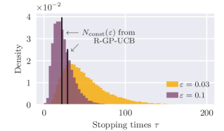
Figure 4: Distribution of stopping times from Definition 3 for $\varepsilon\in\{0.03,0.1\}$ (orange and violet, respectively) using ET-GP-UCB. The vertical solid lines show the constant periodic reset time by R-GP-UCB for the same $\varepsilon$ ($\varepsilon=0.03$ on the right, $\varepsilon=0.1$ on the left).

Furthermore, for a non-changing objective function ($\varepsilon=0$), our bounds recover the known result of a sub-linear regret of standard GP-UCB as $\tilde{\mathcal{O}}(\sqrt{T})$ in Srinivas et al. (2010, Theorem 2).

Empirical Distribution of the Stopping Time

Since the regret bound depends on the stopping time $\tau$ instead of the periodic resets of R-GP-UCB (with $N_{\text{const}}=\lceil\min\{T,12\varepsilon^{-1/4}\}\rceil$ (Bogunovic, Scarlett, and Cevher 2016, Proposition 4.1)), we compare both in Fig. 4. We ran Monte Carlo simulations with ET-GP-UCB on objective functions following Assumption 2 with a fixed set of parameters (listed in Appendix G). We observe that for ET-GP-UCB the time between reset can vary significantly as it does not consider the expected changes (as in R-GP-UCB) but rather the realized changes. Intuitively, if the change is smaller then the expected change, it is beneficial to delay resetting, while the converse is true if the change is bigger. By utilizing this whole distribution of $\tau$, ET-GP-UCB outperforms R-GP-UCB as demonstrated in Sec. 5 even without prior knowledge of the rate of change.

7 Conclusion and Outlook

This paper presents the novel concept of event-triggered resets to optimize time-varying objective functions with TVBO. Based on this concept, we developed the algorithm ET-GP-UCB. It can adapt to the realized changes in the objective function and, crucially, does not depend on any prior knowledge of these temporal changes. This makes ET-GP-UCB especially useful in real-world scenarios. We empirically demonstrated that its adaptive resetting always outperforms periodic resetting. We further showed ET-GP-UCBs superior performance on real-world benchmarks; all without relying on an estimation of the rate of change. To end, we provided regret bounds under common regularity assumption leveraging novel bounds on the model mismatch. Promising future research directions are the design of different event-triggers and the consideration of other changes to the dataset, rather than performing a full reset once the event-trigger is activated; this could help to retain valuable information and thus reduce regret especially for higher dimensional problems. Also of interest is the study of ET-GP-UCB under frequentist regularity assumptions with a fixed variational budget.

Following is the technical appendix for the paper of Event-Triggered Time-Varying Bayesian Optimization. This includes:

• A empirical comparison to the finite variational budget setting

• A sensitivity analysis of the event-trigger hyperparameter $\delta_{\mathrm{B}}$ of ET-GP-UCB

• The proofs of Lemma 2, Lemma 3, and Lemma 4

• The proof of Theorem 1

• Improved regret bounds of R-GP-UCB

• The normalized temperature data for all days used

• An overview of the hyperparameters used in all experiments

Note that all citations here are in the bibliography of the main document, and similarly for many of the cross-references.

Appendix A Comparisons to Algorithms in the Finite Variational Budget Setting

In this section of the appendix, we compare ET-GP-UCB to W-GP-UCB (Deng et al. 2022), and BR-GP-UCB and SW-GP-UCB (Zhou and Shroff 2021). As discussed in Sec. 3, their underlying assumptions differ from ours in that they assume a fixed variational budget. Therefore, a theoretical comparison is not reasonable, but an empirical comparison, especially on real-world data, is interesting. As the baseline that does not consider time-variations, we compare also against IGP-UCB (Chowdhury and Gopalan 2017), which is an improved form of the agnostic GP-UCB of Srinivas et al. (2010). For the comparison, we use the code base submitted by Deng et al. (2022) in the supplementary material of https://proceedings.mlr.press/v151/deng22b. Their experiments consist of:

• an one-dimensional experiment with sudden changes at time steps $t=100$ and $t=200$,

• an one-dimensional experiment with a slowly changing objective function,

• an experiment on real-world stock market data.

We refer to Deng et al. (2022) for the details on how the objective function for (a) and (b) is composed. We implemented our algorithm ET-GP-UCB in their Matlab code base and added random search as a baseline.

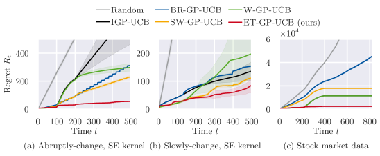
Figure 5: Performance using the refactored GP prior in the experiments of Deng et al. (2022).

While going through the implementation details, we noted that in the stock market data benchmark, the data was not normalized and values of the objective function ranged from $19$ to $250$. This is problematic as all algorithms use a prior mean of zero and a prior variance of one. Thus, all observations will have a very small likelihood under the given model. Secondly, the noise variance was set to $300$, which seems high for stock data where observation noise should be low. The high noise variance combined with the prior signal variance of one also explains the very high standard deviations of all the algorithms in Deng et al. (2022, Figure 1 (c)). Overall, the stock market data has a very low marginal likelihood for the model chosen in (Deng et al. 2022). We, therefore, decided to improve the model and add a preprocessing step to the stock market data example by normalizing the data to a mean of zero and a variance of one to fit the prior model assumptions of all algorithms. Next, we chose a noise variance of $0.01$ to account for smaller short term fluctuations in stock prices. We also changed the noise variance of the synthetic experiments (a) and (b) to $0.1$. It was previously set to $1$ (same as the signal variance), amounting to a ’signal to noise ratio’ of $1$, which is very low for practical optimization problems. We then re-ran their experiments using $20$ runs for the synthetic experiments and $5$ runs for the stock market data as in Deng et al. (2022). For ET-GP-UCB, we use the same parameters for the event-trigger as in all previous experiments. Note that all other time-varying algorithms rely on specifying the amount of change $B_{T}$ a priori, which is hard to estimate in practice. The results are shown in Fig. 5 and regret at the last time step is listed in Table 1.

We can see that ET-GP-UCB can outperform all baselines in experiments Fig. 5 (a) to (c). Especially in Fig. 5 (a), ET-GP-UCB can detect the sudden changes in the objective function and then quickly find the new optimum due to the simple one-dimensional objective function. In Fig. 5 (b), ET-GP-UCB is the best performing algorithm, but W-GP-UCB is competitive. Considering the good performance of IGP-UCB, we can also conclude that the changes in the objective function over the time horizon are relatively small. In Fig. 5 (c), ET-GP-UCB is again the best-performing algorithm. We also observe that in Fig. 5 (c) all algorithms significantly improve in performance and yield a smaller standard deviation compared to Deng et al. (2022, Figure 1 (c)) because the GP prior model is more suitable for modeling the objective function. After approx. $500$ time steps ET-GP-UCB, W-GP-UCB, SW-GP-UCB, and IGP-UCB (see Table 1), no longer accumulate regret. Looking at the objective function, this is expected as the optimal bandit arm no longer changes and the optimal values do not change significantly.

	(a) Abruptly-change		(b) Slowly-change		(c) Stock market
Algorithm	Regret $(\mu\pm\sigma)$		Regret $(\mu\pm\sigma)$		Regret $(\mu\pm\sigma)$
IGP-UCB	$\quad 704.6$	$\pm 238.9$	$\quad 136.0$	$\pm 32.2$	$11\,462.3$	$\pm 56.0$
BR-GP-UCB	$312.5$	$\pm 4.3$	$153.9$	$\pm 11.0$	$45\,362.2$	$\pm 430.1$
SW-GP-UCB	$233.2$	$\pm 9.1$	$111.6$	$\pm 15.7$	$17\,854.9$	$\pm 27.9$
W-GP-UCB	$298.8$	$\pm 27.3$	$197.0$	$\pm 29.7$	$11\,461.3$	$\pm 32.9$
ET-GP-UCB (ours)	$\bm{55.8}$	$\pm 2.7$	$\bm{86.3}$	$\pm 42.8$	$\bm{2\,483.8}$	$\pm 39.8$

Table 1: Comparison on experiments in Deng et al. (2022).

Results with the Original Gaussian Process Prior

Below in Fig. 6 are the results using the original GP prior from (Deng et al. 2022). We can observe that for Fig. 6 (a), ET-GP-UCB can reliably detect the first change in the objective function at $t=100$. However, due to the low signal-to-noise ratio, ET-GP-UCB can only detect the second change approx. $50\%$ of the time. It is still able to outperform periodic resetting as well as the sliding window approach. In Fig. 6 (b), ET-GP-UCB shows a similar performance as W-GP-UCB. Both examples, however, highlight that ET-GP-UCB is not as dominant as in previous examples if the signal-to-noise ratio is too low since $\bar{w}_{t}$ will be large relative to $|y_{t}-\mu_{\mathcal{D}_{t}}(\bm{x}_{t})|$. For the stock market data, we observe the discussed large standard deviations. All algorithms outperform the random baseline. However, we can observe that the ordering of algorithms has changed compared to Deng et al. (2022, Figure 1 (c)) even though we used their implementations and only added ET-GP-UCB and the random baseline to the run script. Further changing the random seed again changed this ordering of the algorithms which indicates that the prior model assumptions yield random-like behavior as the prior does not allow the GP model to make meaningful decision.

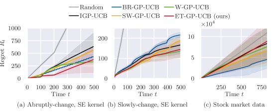
Figure 6: Performance using the original GP prior for the experiments of Deng et al. (2022).

Appendix B Sensitivity of ET-GP-UCB to the Event-Trigger Hyperparameter $\delta_{\mathrm{B}}$

Table 2 shows the sensitivity of ET-GP-UCB to the event-trigger parameter $\delta_{\mathrm{B}}$ in Lemma 3. As $\delta_{\mathrm{B}}$ is increased, the average number of resets increases as the probabilistic uniform error bound is softened. We observe, that for different rate of changes $\varepsilon$ different $\delta_{\mathrm{B}}$ may be optimal to obtain the lowest possible empirical regret. ET-GP-UCB displays a low sensitivity to $\delta_{\mathrm{B}}$ highlighting that our algorithm is readily applicable without the need for excessive hyperparameter tuning. In practice, we found $\delta_{\mathrm{B}}=0.1$ to yield good empirical performance in all of our experiments.

Rate of Change $\varepsilon$	ET-GP-UCB Hyperparameter $\delta_{\mathrm{B}}$	Avg. No. of Resets	Avg. Regret $R_{T}$
	$0.005$	$2.66$	$191.39$
	$0.01$	$2.96$	$193.05$
$0.01$	$0.05$	$3.20$	$200.16$
	$0.1$	$3.38$	$200.33$
	$0.5$	$3.98$	$196.03$
	$0.005$	$6.42$	$276.84$
	$0.01$	$6.82$	$273.37$
$0.03$	$0.05$	$7.72$	$269.01$
	$0.1$	$8.04$	$271.59$
	$0.5$	$10.32$	$280.05$
	$0.005$	$9.60$	$331.69$
	$0.01$	$9.96$	$328.74$
$0.05$	$0.05$	$11.40$	$329.47$
	$0.1$	$11.88$	$332.04$
	$0.5$	$14.44$	$334.80$

Table 2: Sensitivity of ET-GP-UCB to $\delta_{\mathrm{B}}$ in Lemma 3.

Appendix C Proof of Lemma 2, Lemma 3, and Lemma 4

Proof of Lemma 2.

Since $w_{{t^{\prime}}}\sim\mathcal{N}(0,\sigma_{n}^{2})$, we can use a standard bound on the tail probability of the normal distribution $\mathbb{P}\left\{|r|>s\right\}\leq\exp\left\{-s^{2}/(2\sigma^{2})\right\}$ with $r\sim\mathcal{N}(0,\sigma^{2})$ to obtain $\mathbb{P}\left\{|w_{{t^{\prime}}}|\leq\bar{w}_{{t^{\prime}}}\right\}\geq 1-\exp\left\{-\bar{w}_{{t^{\prime}}}^{2}/(2\sigma_{n}^{2})\right\}$. Solving for $\bar{w}_{t}$ with $\delta/\pi_{{t^{\prime}}}$ using the same arguments as in the proof of Srinivas et al. (2010, Lemma 5.5) and taking the union bound over all time steps yields the results. ∎

Proof of Lemma 3.

From Lemma 1 with $\delta_{\mathrm{B}}/2$ and incorporating the noise, we have

$$|f_{t}(\bm{x}_{t})+w_{{t^{\prime}}}-\mu_{\mathcal{D}_{t}}(\bm{x}_{t})| \leq\sqrt{\rho_{{t^{\prime}}}}\sigma_{\mathcal{D}_{t}}(\bm{x}_{t})+|w_{{t^{\prime}}}|$$

$$|y_{t}-\mu_{\mathcal{D}_{t}}(\bm{x}_{t})| \leq\sqrt{\rho_{{t^{\prime}}}}\sigma_{\mathcal{D}_{t}}(\bm{x}_{t})+|w_{{t^{\prime}}}|.$$ (14)

with $\rho_{{t^{\prime}}}=2\ln{\frac{2\pi_{{t^{\prime}}}}{\delta_{\mathrm{B}}}}$. Using Lemma 2 with $\delta_{\mathrm{B}}/2$ and taking the union bound yields the result. ∎

Proof of Lemma 4.

We can use Markov’s inequality to prove the claim, as $\tau$ is a non-negative random variable. ∎

Appendix D Proof of Theorem 1

The proof of Theorem 1 uses similar concepts as Bogunovic, Scarlett, and Cevher (2016) and Srinivas et al. (2010) with the key distinction, that we will explicitly include the event-trigger and its stopping time into our proof. As in Bogunovic, Scarlett, and Cevher (2016) and Srinivas et al. (2010), we first fix a discretization $\mathbb{X}_{t}\subset\mathbb{X}\subseteq[0,r]^{d}$ of size $(\vartheta_{t})^{d}$ satisfying

$$\|\bm{x}-[\bm{x}]_{t}\|\leq\,rd/\vartheta_{t},\quad\forall\bm{x}\in\mathbb{X}_{t}$$ (15)

where $[\bm{x}]_{t}$ denotes the closest point in $\mathbb{X}_{t}$ to $\bm{x}$. Now fix a constant $\delta>0$ and an increasing sequence of positive constants $\{\pi_{t}\}_{t=1}^{\infty}$ satisfying $\sum_{t\geq 1}\pi_{t}^{-1}=1$ (cf. Remark Remark). Next, we introduce three Lemmas needed to bound the regret.

Lemma 5 (Bogunovic, Scarlett, and Cevher (2016, Proof of Theorem 4.2)).

Pick $\delta\in(0,1)$ and set $\beta_{t}=2\ln\frac{\pi_{t}}{\delta}$, where $\sum_{t\geq 1}\pi_{t}^{-1}=1$, $\pi_{t}>0$. Then we have

$$\mathbb{P}\left\{|f_{t}(\bm{x}_{t})-\tilde{\mu}_{\mathcal{D}_{t}}(\bm{x}_{t})|\leq\,\sqrt{\beta_{t}}\tilde{\sigma}_{\mathcal{D}_{t}}(\bm{x}_{t}),\quad\forall t\geq 1\right\}\geq 1-\delta.$$ (16)

Proof.

Bogunovic, Scarlett, and Cevher (2016, Appendix C.1). ∎

Lemma 6.

Pick $\delta\in(0,1)$ and set $\bar{y}_{t}=(b_{0}+\sqrt{2}\sigma_{n})\sqrt{\ln\frac{2(a_{0}+1)\pi_{t}}{\delta}}$, where $\sum_{t\geq 1}\pi_{t}^{-1}=1$, $\pi_{t}>0$. Then we have

$$\mathbb{P}\left\{|y_{t}|\leq\,\bar{y}_{t},\,\forall t\geq 1\right\}\geq 1-\delta.$$ (17)

Proof.

We have that $|y_{t}|\leq\,|f_{t}(\bm{x}_{t})|+|w_{t}|$ given Assumption 1. We can use Lemma 2 (with $t$ instead of $t^{\prime}$) with $\delta/2$ to bound $|w_{t}|$ for all time steps. Combined with Assumption 3 we have

$$\mathbb{P}\left\{|y_{t}|\leq\,L_{f}+\bar{w}_{t}\right\}\geq 1-a_{0}\exp\{-L_{f}^{2}/b_{0}^{2}\}-\delta/2.$$ (18)

Solving the remaining term with $\delta/2$ and using the union bound, we get $\bar{y}^{\prime}_{t}=L_{f}+\bar{w}_{t}\coloneqq b_{0}\sqrt{\ln\frac{2a_{0}\pi_{t}}{\delta}}+\bar{w}_{t}.$ Here, we can further bound $b_{0}\sqrt{\ln\frac{2a_{0}\pi_{t}}{\delta}}$ with $b_{0}\sqrt{\ln\frac{2(a_{0}+1)\pi_{t}}{\delta}}$ using the monotonicity of the logarithm (recall that $a_{0}>0$). Since we have $\bar{w}_{t}=\sqrt{2}\sigma_{n}\sqrt{\ln\frac{2\pi_{t}}{\delta}}$, we can use the same trick to state that $\bar{w}_{t}\leq\sqrt{2}\sigma_{n}\sqrt{\ln\frac{2(a_{0}+1)\pi_{t}}{\delta}}$. To end, we can concatenate the terms obtaining $\bar{y}^{\prime}_{t}\leq\bar{y}_{t}\coloneqq(b_{0}+\sqrt{2}\sigma_{n})\sqrt{\ln\frac{2(a_{0}+1)\pi_{t}}{\delta}}$ proving the claim. ∎

Lemma 7 (Bogunovic, Scarlett, and Cevher (2016, Proof of Theorem 4.2)).

Pick $\delta\in(0,1)$ and set

$$\beta_{t}=2\ln\left(\frac{2\pi_{t}}{\delta}\right)+2d\ln{\left(rdt^{2}b_{1}\sqrt{\ln(2a_{1}d\pi_{t}/\delta)}\right)},$$

where $\sum_{t\geq 1}\pi_{t}^{-1}=1$, $\pi_{t}>0$. Let $\vartheta_{t}=rdt^{2}b_{1}\sqrt{\ln(2a_{1}d\pi_{t}/\delta)}$ and let $[\bm{x}^{*}]_{t}$ be the closest point in $\mathbb{X}_{t}$ to $\bm{x}^{*}$. Then we have

$$\mathbb{P}\left\{|f_{t}(\bm{x}_{t}^{*})-\tilde{\mu}_{\mathcal{D}_{t}}([\bm{x}_{t}^{*}]_{t})|\leq\,\sqrt{\beta_{t}}\tilde{\sigma}_{\mathcal{D}_{t}}([\bm{x}_{t}^{*}]_{t})+\frac{1}{t^{2}},\,\,\forall t\geq 1\right\}\geq 1-\delta.$$ (19)

Proof.

In Bogunovic, Scarlett, and Cevher (2016, Appendix C.1) using Assumption 3 on the kernel function. ∎

For Theorem 1, we condition on four high probability events i.e., Lemma 4, Lemma 5, Lemma 6, and Lemma 7 each with with $\delta/4$. We will explicitly highlight the usage of each Lemma. We can bound the instantaneous regret at a time step $t$ as

$$r_{t} =f_{t}(\bm{x}_{t}^{*})-f_{t}(\bm{x}_{t})$$ (20)

$$\leq\,\tilde{\mu}_{\mathcal{D}_{t}}([\bm{x}_{t}^{*}]_{t})+\sqrt{\beta_{t}}\tilde{\sigma}_{\mathcal{D}_{t}}([\bm{x}_{t}^{*}]_{t})+\frac{1}{t^{2}}-\tilde{\mu}_{\mathcal{D}_{t}}(\bm{x}_{t})+\sqrt{\beta_{t}}\tilde{\sigma}_{\mathcal{D}_{t}}(\bm{x}_{t}).\qquad\text{(Lemma~{}\ref{lem:xt_bound}, Lemma~{}\ref{lem:disc_bound})}$$ (21)

This is identical to Bogunovic, Scarlett, and Cevher (2016, Proof of Theorem 4.2) for R-GP-UCB. We now account for model mismatch between using the time-invariant model in the algorithm and the “true” time-varying posterior as

$$\tilde{\mu}_{\mathcal{D}_{t}}(\bm{x}) \leq\,\mu_{\mathcal{D}_{t}}(\bm{x})+\Delta_{\mathcal{D}_{t}}^{(\mu)}\qquad\text{with}\quad\Delta_{\mathcal{D}_{t}}^{(\mu)}\coloneqq\sup_{\bm{x}\in\mathbb{X}}\left\{|\tilde{\mu}_{\mathcal{D}_{t}}(\bm{x})-\mu_{\mathcal{D}_{t}}(\bm{x})|\right\}$$ (22)

$$\tilde{\sigma}_{\mathcal{D}_{t}}(\bm{x}) \leq\,\sigma_{\mathcal{D}_{t}}(\bm{x})+\Delta_{\mathcal{D}_{t}}^{(\sigma)}\qquad\text{with}\quad\Delta_{\mathcal{D}_{t}}^{(\sigma)}\coloneqq\sup_{\bm{x}\in\mathbb{X}}\left\{|\tilde{\sigma}_{\mathcal{D}_{t}}(\bm{x})-\sigma_{\mathcal{D}_{t}}(\bm{x})|\right\}.$$ (23)

We can thus further bound the regret as

$$r_{t}\leq\,\, \mu_{\mathcal{D}_{t}}([\bm{x}_{t}^{*}]_{t})+\Delta_{\mathcal{D}_{t}}^{(\mu)}([\bm{x}_{t}^{*}]_{t})+\sqrt{\beta_{t}}\left(\sigma_{\mathcal{D}_{t}}([\bm{x}_{t}^{*}]_{t})+\Delta_{\mathcal{D}_{t}}^{(\sigma)}([\bm{x}_{t}^{*}]_{t})\right)$$ (24)

$$-\mu_{\mathcal{D}_{t}}(\bm{x}_{t})+\Delta_{\mathcal{D}_{t}}^{(\mu)}(\bm{x}_{t})+\sqrt{\beta_{t}}\left(\sigma_{\mathcal{D}_{t}}(\bm{x}_{t})+\Delta_{\mathcal{D}_{t}}^{(\sigma)}(\bm{x}_{t})\right)+\frac{1}{t^{2}}.$$ (25)

Per definition of Algorithm 1, we have that through the optimization of its UCB-type acquisition function $\mu_{\mathcal{D}_{t}}([\bm{x}_{t}^{*}]_{t})+\sqrt{\beta_{t}}\sigma_{\mathcal{D}_{t}}([\bm{x}_{t}^{*}]_{t})\leq\,\mu_{\mathcal{D}_{t}}(\bm{x}_{t})+\sqrt{\beta_{t}}\sigma_{\mathcal{D}_{t}}(\bm{x}_{t})$, and, therefore,

$$r_{t}\leq\, 2\sqrt{\beta_{t}}\sigma_{\mathcal{D}_{t}}(\bm{x}_{t})+\frac{1}{t^{2}}+\Delta_{\mathcal{D}_{t}}^{(\mu)}([\bm{x}_{t}^{*}]_{t})+\Delta_{\mathcal{D}_{t}}^{(\mu)}(\bm{x}_{t})+\sqrt{\beta_{t}}\left(\Delta_{\mathcal{D}_{t}}^{(\sigma)}([\bm{x}_{t}^{*}]_{t})+\Delta_{\mathcal{D}_{t}}^{(\sigma)}(\bm{x}_{t})\right).$$ (26)

What is left to bound is the model mismatch. Instead of using the same bounds as in Bogunovic, Scarlett, and Cevher (2016, Proof of Theorem 4.2 (R-GP-UCB)) by applying Bogunovic, Scarlett, and Cevher (2016, Lemma D.1.) with $|\mathcal{D}_{t}|<\bar{\tau}$ (Lemma 4), we next present novel bounds on the maximum model mismatch defined in (22) and (23). Note, that other bounds on the model mismatch are possible e.g., using the fact that the output of the kernel function is bounded by one. Such ‘trivial’ bounds, however, would loose the desirable explicit dependency of the model mismatch and $\varepsilon$ (cf. black line in Fig. 7).

Lemma 8.

Conditioned on the event in Lemma 6, we have for any block size $N$ that the maximum model mismatch in the mean and variance between the time-varying GP model and the time-invariant GP model is a.s. bounded as

$$\Delta_{\mathcal{D}_{t}}^{(\sigma)} \leq\sqrt{\left(3\sigma_{n}^{-2}+\sigma_{n}^{-4}\right)N^{2}\left(1-e^{-p(\varepsilon)N}\right)}$$ (27)

$$\Delta_{\mathcal{D}_{t}}^{(\mu)} \leq\left(\sigma_{n}^{-2}+\sigma_{n}^{-4}\right)N^{2}\left(1-e^{-p(\varepsilon)N}\right)\bar{y}_{N}$$ (28)

where $p(\varepsilon)=-\frac{1}{2}\ln{(1-\varepsilon)}$ and $\bar{y}_{N}=(b_{0}+\sqrt{2}\sigma_{n})\sqrt{\ln\frac{2(a_{0}+1)\pi^{2}N^{2}}{\delta}}$.

Proof.

The proof of this Lemma follows the same argumentation to the one of Bogunovic, Scarlett, and Cevher (2016, Lemma D.1.). It differs in bounding the term $||\tilde{\bm{k}}_{t}(\bm{x})-\bm{k}_{t}(\bm{x})||_{2}$ not with the infinity norm using a linearized form of the maximum value of the entries of the vector as $N\varepsilon$ but rather using the actual maximum value as $\left(1-e^{-p(\varepsilon)N}\right)$. For completeness, we provide the full proof for (27). The arguments for (28) are essentially but using this actual bound. For convenience, we use the shorthand notation $\bm{k}\coloneqq\bm{k}_{t}(\bm{x})$, $\textbf{K}\coloneqq\textbf{K}_{t}$, $\tilde{\bm{k}}\coloneqq\ \tilde{\bm{k}}_{t}$, and $\tilde{\textbf{K}}\coloneqq\tilde{\textbf{K}}_{t}$. As in Bogunovic, Scarlett, and Cevher (2016, Lemma D.1.), we first use (6) and (8) and the triangle inequality to write

$$|\tilde{\sigma}_{\mathcal{D}_{t}}^{2}(\bm{x})-\sigma_{\mathcal{D}_{t}}^{2}(\bm{x})| =\left|\tilde{\bm{k}}^{T}(\tilde{\textbf{K}}+\sigma_{n}^{2}\textbf{I})^{-1}\tilde{\bm{k}}-\bm{k}^{T}(\textbf{K}+\sigma_{n}^{2}\textbf{I})^{-1}\bm{k}\right|$$ (29)

$$\leq\left|\tilde{\bm{k}}^{T}(\tilde{\textbf{K}}+\sigma_{n}^{2}\textbf{I})^{-1}\tilde{\bm{k}}-\tilde{\bm{k}}^{T}(\textbf{K}+\sigma_{n}^{2}\bm{I})^{-1}\tilde{\bm{k}}\right|+\left|\tilde{\bm{k}}^{T}(\textbf{K}+\sigma_{n}^{2}\bm{I})^{-1}\tilde{\bm{k}}-\bm{k}^{T}(\textbf{K}+\sigma_{n}^{2}\textbf{I})^{-1}\bm{k}\right|$$ (30)

$$\eqqcolon T_{1}+T_{2}.$$ (31)

Lets first consider $T_{2}$ and define $M\coloneqq(\textbf{K}+\sigma_{n}^{2}\textbf{I})^{-1}$. Now by expanding the quadratic function, regrouping terms and then applying the triangle inequality, we obtain

$$T_{2}\leq 2\left|\bm{k}^{T}\textbf{M}(\tilde{\bm{k}}-\bm{k})\right|+\left|(\tilde{\bm{k}}-\bm{k})^{T}\textbf{M}(\tilde{\bm{k}}-\bm{k})\right|.$$ (32)

The remaining part of the proof focuses on bounding the individual terms $\bm{a}^{T}\textbf{M}\bm{b}$ by $\|\bm{a}||_{2}||\textbf{M}||_{2\to 2}||\bm{b}||_{2}$. Here, it is known that $||\textbf{M}||_{2\to 2}\leq\frac{1}{\sigma_{n}^{2}}$. Since the entries of $\bm{k}$ are in $[0,1]$, we have that $\|\bm{k}\|_{2}\leq N$ using the fact that the Euclidean norm is upper-bounded as $\|\cdot\|_{2}\leq N\|\cdot\|_{\infty}$. Lastly, we have to bound $\|\bm{k}-\tilde{\bm{k}}\|_{2}$. As discussed, the entries of $\bm{k}$ are bounded by $1$. Now note, that the entries $\tilde{k}_{i}$ of $\tilde{\bm{k}}$ are bounded as $1\cdot(1-\varepsilon)^{i/2}$ using the fact that $\bm{k}^{\text{time}}$ is known. Therefore,

$$\|\bm{k}-\tilde{\bm{k}}\|_{2}\leq N\|\bm{k}-\tilde{\bm{k}}\|_{\infty}\leq N\left(1-(1-\varepsilon)^{N/2}\right)=N\left(1-e^{-p(\varepsilon)N}\right)$$ (33)

with $p(\varepsilon)=-\frac{1}{2}\ln{(1-\varepsilon)}$. Using this, we can bound $T_{2}$ as

$$T_{2}\leq 2\sigma_{n}^{-2}N\left(1-e^{-p(\varepsilon)N}\right)+\sigma_{n}^{-2}N^{2}\left(1-e^{-p(\varepsilon)N}\right)^{2}.$$ (34)

For $T_{1}$, using the same arguments as in Bogunovic, Scarlett, and Cevher (2016, Equations (78-80)) and the improved bound on $\|\bm{k}-\tilde{\bm{k}}\|_{2}$, we get that $T_{1}\leq\sigma_{n}^{-4}N^{2}\left(1-e^{-p(\varepsilon)N}\right)$ and thus

$$|\tilde{\sigma}_{\mathcal{D}_{t}}^{2}(\bm{x})-\sigma_{\mathcal{D}_{t}}^{2}(\bm{x})|\leq T_{1}+T_{2} \leq\sigma_{n}^{-4}N^{2}\left(1-e^{-p(\varepsilon)N}\right)+2\sigma_{n}^{-2}N\left(1-e^{-p(\varepsilon)N}\right)+\sigma_{n}^{-2}N^{2}\left(1-e^{-p(\varepsilon)N}\right)^{2}$$ (35)

$$\leq\left(3\sigma_{n}^{-2}+\sigma_{n}^{-4}\right)N^{2}\left(1-e^{-p(\varepsilon)N}\right).$$ (36)

With $a-b\leq\sqrt{|a^{2}-b^{2}|}$, we then obtain the claim in (27). With the same argumentation, we can prove the claim in (28) but using the fact that $\|\bm{y}\|_{2}\leq N\bar{y}_{N}$ as we conditioned on the event from Lemma 6. ∎

To highlight that the bounds in Lemma 8 are indeed tighter that previous ones, we provide a comparison in Fig. 7 for different $\varepsilon$ for $\Delta_{t}^{(\sigma)}$. Here, the solid black line indicates using a ‘trivial’ bound on $\|\bm{k}-\tilde{\bm{k}}\|_{2}$ as $\|\bm{k}-\tilde{\bm{k}}\|_{2}\leq N$. Note that by doing this, one would loose the dependency of the bounds on $\varepsilon$ and thus also loose the desirable explicit of the regret and $\varepsilon$. In Fig. 7, we can observe the both bounds on the model mismatch, our improved ones and the one in Bogunovic, Scarlett, and Cevher (2016, Lemma D.1.), converge to $0$ for $\varepsilon=0$. We can further see that the improved bound is tighter for all $\varepsilon$. While the previous bound quickly becomes worse compared to the ‘trivial’ bound as $N$ or $\varepsilon$ increase, we can observe that our improved bound is always upper bounded by this ‘trivial’ bound, converging to it as $N$ increases (see e.g., $\varepsilon=0.3$).

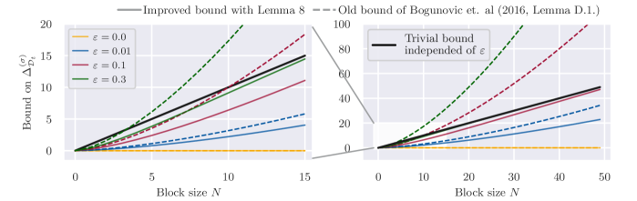
Figure 7: Visualization of our improved bounds on the maximum model mismatch. The solid black line indicates using a ‘trivial’ bound on $\|\bm{k}-\tilde{\bm{k}}\|_{2}$ as $\|\bm{k}-\tilde{\bm{k}}\|_{2}\leq N$. Our improved bound (solid lines with color) is tighter than previous results (dashed lines) for all $\varepsilon$. Furthermore, instead of becoming worse than the ‘trivial’ bound, the improved bounds are upper bounded by it.

Coming back to the proof of Theorem 1 and using Lemma 8, we can summarize the bound on the model mismatch at each time step as

$$2\Delta_{\mathcal{D}_{t}}^{(\mu)}+2\sqrt{\beta_{t}}\Delta_{\mathcal{D}_{t}}^{(\sigma)}\leq\,2\left(\sigma_{n}^{-2}+\sigma_{n}^{-4}\right)\bar{\tau}^{2}\left(1-e^{-p(\varepsilon)\bar{\tau}}\right)\bar{y}_{\bar{\tau}}+2\sqrt{\beta_{t}\left(3\sigma_{n}^{-2}+\sigma_{n}^{-4}\right)\bar{\tau}^{2}\left(1-e^{-p(\varepsilon)\bar{\tau}}\right)}\eqqcolon\phi_{t}(\varepsilon,\delta,\bar{\tau})$$ (37)

For completeness, we follow the step in Srinivas et al. (2010, Proof of Theorem 2) and Bogunovic, Scarlett, and Cevher (2016, Proof of Theorem 4.2 (R-GP-UCB)) to bound the regret following Def. 1 as

$$R_{T}\coloneqq\sum_{t=1}^{T}r_{t}\leq\,\sum_{t=1}^{T}2\sqrt{\beta_{t}}\sigma_{\mathcal{D}_{t}}(\bm{x}_{t})+\frac{1}{t^{2}}+\phi_{t}(\varepsilon,\delta,\bar{\tau}).$$ (38)

With $\sum_{t=1}^{\infty}1/t^{2}=\pi^{2}/6\leq\,2$ and using Cauchy-Schwarz with $\left(\sum_{t=1}^{T}\bm{x}_{t}\right)^{2}\leq\,T\sum_{t=1}^{T}\bm{x}_{t}^{2}$ we obtain

$$R_{T}\leq\,\sqrt{T\sum_{t=1}^{T}4\beta_{t}\sigma_{\mathcal{D}_{t}}^{2}(\bm{x}_{t})}+2+\sum_{t=1}^{T}\left(2\left(\sigma_{n}^{-2}+\sigma_{n}^{-4}\right)\bar{\tau}^{2}\left(1-e^{-p(\varepsilon)\bar{\tau}}\right)\bar{y}_{\bar{\tau}}+2\sqrt{\beta_{t}\left(3\sigma_{n}^{-2}+\sigma_{n}^{-4}\right)\bar{\tau}^{2}\left(1-e^{-p(\varepsilon)\bar{\tau}}\right)}\right).$$ (39)

Furthermore, using the same arguments as in Bogunovic, Scarlett, and Cevher (2016, Proof of Theorem 4.2 (R-GP-UCB)) and Srinivas et al. (2010, Proof of Lemma 5.3 (GP-UCB)) on the information gain within a block of size $M$ is $I(y_{M};f_{M})=\frac{1}{2}\sum_{t=1}^{M}\ln\left(1+\sigma_{n}^{-2}\sigma_{\mathcal{D}_{t}}^{2}(\bm{x}_{t})\right)\leq\,\gamma_{M}$ with $\gamma_{M}=\max_{\bm{x}_{1},\dots\bm{x}_{\tau}}I(y_{M};f_{M})$ yields:

$$\sum_{t=1}^{T}4\beta_{t}\sigma_{\mathcal{D}_{t}}^{2}(\bm{x}_{t}) \leq\,4\beta_{T}\sigma_{n}^{2}\sum_{t=1}^{T}\left(\sigma_{n}^{-2}\sigma_{\mathcal{D}_{t}}^{2}(\bm{x}_{t})\right)$$ (40)

$$\leq\,4\beta_{T}\sigma_{n}^{2}C_{2}\sum_{t=1}^{T}\ln\left(1+\sigma_{n}^{-2}\sigma_{\mathcal{D}_{t}}^{2}(\bm{x}_{t})\right)$$ (41)

with $$C_{2}=\sigma_{n}^{-2}/\ln(1+\sigma_{n}^{-2})\geq 1 s^{2}\leq\,C_{2}\ln(1+s^{2}) s\in[0,\sigma_{n}^{2}] \sigma_{n}^{-2}\sigma_{\mathcal{D}_{t}}^{2}(\bm{x}_{t})\leq\,\sigma_{n}^{-2}k(\bm{x}_{t},\bm{x}_{t})\leq\,\sigma_{n}^{-2}$$, since for , and due to the bounded kernel function in Assumption 2 (also see Srinivas et al. (2010, Proof of Lemma 5.4), we get

$$\leq\,8\beta_{T}\sigma_{n}^{2}C_{2}\frac{T}{\bar{\tau}}I(y_{\bar{\tau}};f_{\bar{\tau}})\qquad\text{($\frac{T}{\bar{\tau}}$ blocks of $I(y_{\bar{\tau}};f_{\bar{\tau}})$ in $T$)}$$ (42)

$$\leq\,8\beta_{T}\sigma_{n}^{2}C_{2}\frac{T}{\bar{\tau}}\gamma_{\bar{\tau}}$$ (43)

We assumed that $\frac{T}{\bar{\tau}}$ is an integer as the number of block in $T$ and we can upper this with $\big{(}\frac{T}{\bar{\tau}}+1\big{)}$. Therefore, we have

$$R_{T}\leq\,\sqrt{C_{1}T\beta_{T}\left(\frac{T}{\bar{\tau}}+1\right)\gamma_{\bar{\tau}}}+2+\sum_{t=1}^{T}\left(2\left(\sigma_{n}^{-2}+\sigma_{n}^{-4}\right)\bar{\tau}^{2}\left(1-e^{-p(\varepsilon)\bar{\tau}}\right)\bar{y}_{\bar{\tau}}+2\sqrt{\beta_{t}\left(3\sigma_{n}^{-2}+\sigma_{n}^{-4}\right)\bar{\tau}^{2}\left(1-e^{-p(\varepsilon)\bar{\tau}}\right)}\right)$$ (44)

with $C_{1}=8/\ln(1+\sigma_{n}^{-2})$. Further bounding the sum over maximum model mismatch with $\beta_{t}\leq\,\beta_{T}$ for all $t$ yields

$$R_{T} \leq\,\sqrt{C_{1}T\beta_{T}\left(\frac{T}{\bar{\tau}}+1\right)\gamma_{\bar{\tau}}}+2+T\left(\underbrace{2\left(\sigma_{n}^{-2}+\sigma_{n}^{-4}\right)\bar{\tau}^{2}\left(1-e^{-p(\varepsilon)\bar{\tau}}\right)\bar{y}_{\bar{\tau}}+2\sqrt{\beta_{T}\left(3\sigma_{n}^{-2}+\sigma_{n}^{-4}\right)\bar{\tau}^{2}\left(1-e^{-p(\varepsilon)\bar{\tau}}\right)}}_{\phi_{T}(\varepsilon,\delta,\bar{\tau})\text{ in Theorem~{}\ref{theorem:regret_bounds}}}\right).$$

$\square$

Appendix E Improved Regret Bounds of R-GP-UCB

Using our improved bounds on the model mismatch, we can provide tighter bounds for R-GP-UCB below.

Theorem 2 (Improved regret bounds for R-GP-UCB).

Let the domain $\mathbb{X}\subset[0,r]^{d}\subset\mathbb{R}^{d}$ be convex and compact with $d\in\mathbb{N}_{+}$ and let $f_{t}$ follow Assumption 2 with a kernel $k(\bm{x},\bm{x}^{\prime})$ such that Assumption 3 is satisfied. Pick $\delta\in(0,1)$ and set

$$\beta_{t}=2\ln\left(2\pi^{2}t^{2}/(3\delta)\right)+2d\ln{\left(t^{2}db_{1}r\sqrt{\ln(2da_{1}\pi^{2}t^{2}/(3\delta))}\right)}.$$ (45)

Then, after running R-GP-UCB (with a fixed periodic reset time $N$) for $T$ time steps,

$$R_{T}\leq\sqrt{C_{1}T\beta_{T}\left(\frac{T}{N}+1\right)\gamma_{N}}+2+T\phi_{T}(\varepsilon,\delta,N)$$ (46)

is satisfied with probability at least $1-\delta$, where ${C_{1}=8/\ln(1+\sigma_{n}^{-2})}$ and we defined

$$\phi_{T}(\varepsilon,\delta,N)\coloneqq 2\sqrt{\beta_{T}(3\sigma_{n}^{-2}+\sigma_{n}^{-4})N^{2}(1-e^{-p(\varepsilon)N})}+2(\sigma_{n}^{-2}+\sigma_{n}^{-4})N^{2}(1-e^{-p(\varepsilon)N})\bar{y}_{N}$$ (47)

where $p(\varepsilon)=-\frac{1}{2}\ln{(1-\varepsilon)}$ and $\bar{y}_{N}=(b_{0}+\sqrt{2}\sigma_{n})\sqrt{\ln\frac{2(a_{0}+1)\pi^{2}\bar{N}^{2}}{3\delta}}$.

Proof.

The proof is the same as in Bogunovic, Scarlett, and Cevher (2016, Proof of Theorem 4.2) but using our improved bounds from Lemma 8 instead of Bogunovic, Scarlett, and Cevher (2016, Lemma D.1) to bound the model mismatch. ∎

Appendix F Overview of the Temperature Data

In Fig. 8, we show the normalized temperature data used for the empirical kernel in the results in Fig. 3. The full pre-processing of the temperature data is described in the corresponding jupyter-notebook in the provided code base.

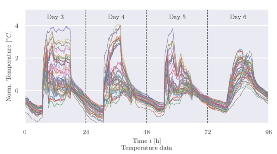
Figure 8: Normalized temperature data used for the results in Fig. 3. Each color resembles the readings from one sensor.

Appendix G Hyperparameters

To ensure the reproducibility of our results, we give a list of all hyperparameters used in any simulation performed for this paper. All experiments in Sec. 5 were conducted on a 2021 MacBook Pro with an Apple M1 Pro chip and 16GB RAM. The Monte Carlo simulations in Sec. 6 were conducted over 3 days on a compute cluster. The temperature data set is publicly available at http://db.csail.mit.edu/labdata/labdata.html. The code will be published upon acceptance and is also part of the supplementary material of the submission.

Hyperparameters	Monte Carlo Simulation
dimension $d$	$2$
compact set $\mathbb{X}$	$[0,1]^{2}$
lengthscales $l$	$0.2$
time horizon $T$	$200$
noise variance $\sigma_{n}^{2}$	$0.02$
number of i.i.d. runs	$30\,000$
event-trigger parameter in Lemma 3 $\delta_{\mathrm{B}}$	$0.1$
rate of change $\varepsilon$	$\{0.03,0.1\}$

Table 3: Hyperparameters of the Monte Carlo Simulation for ET-GP-UCB (cf. Fig. 4).

Algorithm	Hyperparameters	Comparisons (a) to (c)	Comparison (d)
	dimension $d$	$2$	$2$
	compact set $\mathbb{X}$	$[0,1]^{2}$	$[0,1]^{2}$
	lengthscales $l$	$0.2$	$0.2$
all	time horizon $T$	$400$	$400$
	noise variance $\sigma_{n}^{2}$	$0.02$	$0.02$
	$\beta_{t}$ approximation parameters	$c_{1}=0.4,c_{2}=4$	$c_{1}=0.4,c_{2}=4$
	number of i.i.d. runs	$50$	$50$
TV-GP-UCB	rate of change $\varepsilon$	$\{0.01,0.03,0.05\}$	$0.001$
R-GP-UCB	reset time $N_{\text{const}}$	$\{38,29,26\}$	$68$
ET-GP-UCB	event-trigger parameter $\delta_{\mathrm{B}}$	$0.1$	$0.1$

Table 4: Hyperparameters for the within-model comparisons (cf. Fig. 2).

Algorithm	Hyperparameters	Temperature Dataset
	dimension $d$	$1$
	compact set $\mathbb{X}$	46 arms
	kernel $k$	empirical kernel
all	time horizon $T$	$286$
	noise variance $\sigma_{n}^{2}$	$0.01$
	$\beta_{t}$ approximation parameters	$c_{1}=0.8,c_{2}=0.4$
	number of i.i.d. runs	$20$
TV-GP-UCB	rate of change $\varepsilon$ (see Bogunovic, Scarlett, and Cevher (2016))	$0.03$
R-GP-UCB	reset time $N_{\text{const}}$ (see Bogunovic, Scarlett, and Cevher (2016))	$15$
ET-GP-UCB	event-trigger parameter in Lemma 3 $\delta_{\mathrm{B}}$	$0.1$

Table 5: Hyperparameters for the temperature dataset (cf. Fig. 3).

Algorithm	Hyperparameters	Policy search
	dimension $d$	$4$
		lower bound to $[-3,-6,-50,-4]$
	compact set $\mathbb{X}$	upper bound to $[-2,-4,-25,-2]$
		scaling factors $[1/8,1/4,3,1/8]$
	lengthscales $l$	Gamma prior $\mathcal{G}(15,10/3)$
all	time horizon $T$	$300$
	noise variance $\sigma_{n}^{2}$	$0.02$
	$\beta_{t}$ approximation parameters	$c_{1}=0.8,c_{2}=4$
	number of i.i.d. runs	$20$
TV-GP-UCB	rate of change $\varepsilon$	$0.03$
R-GP-UCB	reset time $N_{\text{const}}$ induced by rate of change $\varepsilon$	$29$
UI-TVBO	rate of change $\hat{\sigma}_{w}^{2}$	$0.03$
ET-GP-UCB	event-trigger parameter in Lemma 3 $\delta_{\mathrm{B}}$	$0.1$

Table 6: Hyperparameters for the policy search experiment (cf. Fig. 3).

Algorithm	Hyperparameters	Synthetic Experiments
	dimension $d$	$1$
	compact set $\mathbb{X}$	$[0,1]^{2}$
	kernel $k$	fixed, $l=0.2$
	time horizon $T$	$500$
	noise variance $\sigma_{n}^{2}$	$\{0.01,1\}$
	number of i.i.d. runs	$20$
ET-GP-UCB	event-trigger parameter in Lemma 3 $\delta_{\mathrm{B}}$	$0.1$

Table 7: Hyperparameters for the synthetic experiments in Deng et al. (2022).

Algorithm	Hyperparameters	Stock Market Data
	dimension $d$	$1$
	compact set $\mathbb{X}$	$48$ arms
	kernel $k$	empirical kernel
	time horizon $T$	$823$
	noise variance $\sigma_{n}^{2}$	$\{0.01,300\}$
	number of i.i.d. runs	$20$
ET-GP-UCB	event-trigger parameter in Lemma 3 $\delta_{\mathrm{B}}$	$0.1$

Table 8: Hyperparameters for the stock market data experiment in Deng et al. (2022).

Algorithm	Hyperparameters	Sensitivity Analysis
	dimension $d$	$2$
	compact set $\mathbb{X}$	$[0,1]^{2}$
	kernel $k$	fixed, $l=0.2$
all	time horizon $T$	$400$
	noise variance $\sigma_{n}^{2}$	$0.02$
	$\beta_{t}$ approximation parameters	$c_{1}=0.4,c_{2}=4$
	number of i.i.d. runs	$50$
ET-GP-UCB	event-trigger parameter in Lemma 3 $\delta_{\mathrm{B}}$	$\{0.005,0.01,0.05,0.1,0.5\}$

Table 9: Hyperparameters for the sensitivity analysis (cf. Table 2).

References

• Balandat etΒ al. (2020) Balandat, M.; Karrer, B.; Jiang, D.Β R.; Daulton, S.; Letham, B.; Wilson, A.Β G.; and Bakshy, E. 2020. BoTorch: A Framework for Efficient Monte-Carlo Bayesian Optimization. In Advances in Neural Information Processing Systems, volumeΒ 33.
• Besbes, Gur, and Zeevi (2015) Besbes, O.; Gur, Y.; and Zeevi, A. 2015. Non-Stationary Stochastic Optimization. Operations Research, 63(5): 1227–1244.