Building Robust Machine Learning Models for Small Chemical Science Data: The Case of Shear Viscosity

Abstract

Shear viscosity, though being a fundamental property of all liquids, is computationally expensive to estimate from equilibrium molecular dynamics simulations. Recently, Machine Learning (ML) methods have been used to augment molecular simulations in many contexts, thus showing promise to estimate viscosity too in a relatively inexpensive manner. However, ML methods face significant challenges - like overfitting, when the size of the data set is small, as is the case with viscosity. In this work, we train seven ML models to predict the shear viscosity of a Lennard-Jones (LJ) fluid, with particular emphasis on addressing issues arising from a small data set. Specifically, the issues related to model selection, performance estimation and uncertainty quantification were investigated. First, we show that the widely used performance estimation procedure of using a single unseen data set shows a wide variability - in estimating the errors on – small data sets. In this context, the common practice of using Cross validation (CV) to select the hyperparameters (model selection) can be adapted to estimate the generalization error (performance estimation) as well. We compare two simple CV procedures for their ability to do both model selection and performance estimation, and find that k-fold CV based procedure shows a lower variance of error estimates. Also, these CV procedures naturally lead to an ensemble of trained ML models. We discuss the role of performance metrics in training and evaluation and propose a method to rank the ML models based on multiple metrics. Finally, two methods for uncertainty quantification - Gaussian Process Regression (GPR) and ensemble method - were used to estimate the uncertainty on individual predictions. The uncertainty estimates from GPR were also used to construct an applicability domain using which the ML models provided more reliable predictions on another small data set generated in this work. Overall, the procedures prescribed in this work, together, lead to robust ML models for small data sets.

I Introduction

Shear viscosity is a fundamental transport property of all fluids.March and Tosi (2002) Understanding its molecular underpinnings would advance our scientific understanding of supercooled liquids,Levashov, Morris, and Egami (2011) magma transport,Giordano, Russell, and Dingwell (2008) mixing of fluids, etc. For example, a good estimate of shear viscosity is crucial to model the earth’s outer core which is believed to be a liquid form of Iron based alloys.de Wijs et al. (1998); Vočadlo (2007) However, in the absence of direct measurements, its estimates from different methods differ by about fourteen orders of magnitude Secco (1995). Hence, a better understanding of the behavior of viscosity from simulations can help address some of these issues. Further, from the point of view of applications, predicting the viscosity of industrially relevant fluids (such as hydrocarbons and carbonates) in-silico would accelerate the progress in energy storage, petroleum, lubricants, chemical processing, pharmaceutical, and many other sectors.Baled et al. (2018); Kontogeorgis et al. (2021)

I.1 Viscosity from Molecular Dynamics simulations

Atomistic Molecular Dynamics (MD) simulations with ab initio or empirical force fields can be used to estimate the viscosity of any liquid, however complex, in silico. Maginn et al. (2019); Hess (2002); Alfè and Gillan (1998); Jamali et al. (2018a); Li et al. (2021); Malosso et al. (2022); Tazi et al. (2012); Wang et al. (2020); Fedosov et al. (2011) While there exists many methods to estimate viscosity from MD simulations, they largely fall into two categories – Equilibrium MD (EMD) Zhang, Otani, and Maginn (2015); Maginn et al. (2019) and Non-Equilibrium MD (NEMD) based methods.Müller-Plathe (1999); Ewen, Heyes, and Dini (2018); Heyes, Dini, and Smith (2018) A comparison between them is beyond the scope of this work and the readers are directed to some excellent works in this area.Hess (2002); Maginn et al. (2019)

Despite the progress in this area,Hess (2002); Stillinger and Debenedetti (2005); Jones and Mandadapu (2012); Kim, Borodin, and Karniadakis (2015); Zhang, Otani, and Maginn (2015); Oliveira and Greaney (2017); Maginn et al. (2019); Heyes, Smith, and Dini (2019); Heyes, Dini, and Smith (2020, 2021); Heyes and Dini (2022); Malosso et al. (2022) the state-of-the-art methods to estimate viscosity accurately from MD simulations require huge computing time especially for viscous fluids, Zhang, Otani, and Maginn (2015); Avula et al. (2021); Kondratyuk and Pisarev (2021); Goloviznina et al. (2021) as it is a collective quantity. This drawback precludes the use of MD simulations in viscosity-based high throughput screening processes in the industry.Baled et al. (2018) Also, force field refinement strategies which use the experimental viscosity as a benchmark require significant effort for the same reason.Gong and Sun (2019) Another important difficulty in estimating viscosity from MD is its sensitive dependence on primary and ancillary simulation setup parameters. Hess showed that ancillary MD run parameters such as the number of independent replicas, numerical precision of the MD engine, neighbor list cutoff, and Ewald sum related parameters have a significant effect on the estimated viscosity value.Hess (2002) Hence, reporting meaningful confidence intervals of viscosity estimates is crucial and is a topic of ongoing research.Hess (2002); Maginn et al. (2019); Kim et al. (2018); Jones and Mandadapu (2012); Kim, Borodin, and Karniadakis (2015) To address these problems related to estimating shear viscosity from MD simulations, we look at alternate approaches using Machine Learning (ML) methods.

I.2 Machine Learning methods

Recently, Machine Learning and Deep Learning (DL) models have started to augment various aspects of MD simulations.Wang, Lamim Ribeiro, and Tiwary (2020); Noé et al. (2020); Karthikeyan and Priyakumar (2021); Bonati, Piccini, and Parrinello (2021); Doerr et al. (2021) More specifically, in the context of using ML methods to predict slowly converging properties of liquids - of which shear viscosity is one - some initial advances have been made. Alam et al. used Neural Networks (NN) and Random Forests (RF) to predict the self diffusion coefficients of particles interacting via Lennard-Jones (LJ) interaction and showed them to be performing better than empirical models.Allers et al. (2020) They also used ML methods to predict the finite size corrections to self diffusion coefficients in binary LJ fluids.Leverant, Harvey, and Alam (2020) Also, several ML models were also used to predict the experimental viscosity and ionic conductivity of ionic liquids using only molecular features.Beckner, Mao, and Pfaendtner (2018); Koutsoukos et al. (2021); Valderrama, Muñoz, and Rojas (2011); Dutt, Ravikumar, and Rani (2013); Paduszyński and Domańska (2014); Fatehi, Raeissi, and Mowla (2017); Baghban, Kardani, and Habibzadeh (2017); Datta, Ramprasad, and Venkatram (2022); Duong et al. (2022) However, to our knowledge, ML methods have not been used to predict shear viscosity derived purely from MD simulations.

The protocols for developing and comparing ML models - especially for chemical science applications - are not yet completely established.Vishwakarma, Sonpal, and Hachmann (2021) There exist a plethora of supervised learning algorithms,Bishop (2006); Goodfellow, Bengio, and Courville (2016) model selection rules,Arlot and Celisse (2010); Cawley and Talbot (2010); Zhang and Yang (2015); Burnham and Anderson (2003); Xu and Goodacre (2018) performance metrics,Vishwakarma, Sonpal, and Hachmann (2021); Armstrong and Collopy (1992); Gneiting (2011) and uncertainty quantification methods Schwaighofer et al. (2007); Tran et al. (2020); Scalia et al. (2020); Imbalzano et al. (2021); Tavazza, DeCost, and Choudhary (2021) which are used to create ML models; yet, there are no clear protocols on which combination should be chosen. For example, among the many performance metrics that are used to train and compare ML models, the best choice is still a matter of debate.Vishwakarma, Sonpal, and Hachmann (2021); Kolassa (2020); Makridakis, Spiliotis, and Assimakopoulos (2020) Similar conclusions hold true for model selection,Xu and Goodacre (2018) and uncertainty quantification Hirschfeld et al. (2020) as well.

In this context, ’No-Free-Lunch’ theorems by Wolpert and Mcready imply that there is no single algorithm that has the best performance across all possible optimization problems.Wolpert and Macready (1997) These theorems when applied to ML indicate that any single ML algorithm cannot be expected to perform well across all possible ML tasks. Though there is still a debate on the applicability of these theorems to practical ML problems, it is considered common knowledge that the ML algorithm should be tailored to the specific task at hand.Goodfellow, Bengio, and Courville (2016) Exploiting the idiosyncrasies of the data set can lead to significant improvements in the performance of ML models. For example, M$\ddot{\rm u}$ller et al. were able to improve the performance (MAE) of ML models used to predict atomization energies from 10 kcal/mol to 3 kcal/mol (70 % improvement) by exploring a number of ML techniques and molecular representations.Hansen et al. (2013) In this work, we use this approach to develop ML models tailored to viscosity data set generated from equilibrium MD simulations.

I.3 ML models for small data

As it is computationally costly to get reliable (including standard errors) estimates of viscosity from atomistic MD, generating large data sets (like GDB-17 with nearly 150 billion data points Ruddigkeit et al. (2012)) is practically infeasible with the current computing resources. The largest MD-derived viscosity data set (with 1061 data points) we could find was the work of Vlugt et al. in which the MD computed viscosity was used to predict the box size corrections to diffusion coefficients of particles in binary Lennard-Jones (LJ) systems.Jamali et al. (2018b) Such small data sets pose unique challenges to the ML methods Schleinitz et al. (2022) - (1) they are hard to generalize, (2) they are susceptible to overfitting, and (3) they tend to underestimate the generalization error.Cawley and Talbot (2010); Varoquaux (2018) For example, Neural Networks (NN) which generally outperform other ML models, struggle in the low data regime.Pinheiro et al. (2021); Hansen et al. (2013); Allers et al. (2021) Also, Casson et al., on surveying over 50 articles on machine learning for autism, have shown that ML models tended to produce overoptimistic results when the sample sizes are small.Vabalas et al. (2019) All these issues exacerbate the reproducibility of the results which is already a fast growing challenge in all fields using ML methods.Walters (2013); Heil et al. (2021); Kapoor and Narayanan (2022)

In this work, we train seven ML models to predict the shear viscosity of binary LJ fluids, with particular emphasis on addressing issues arising from a small data set. Specifically, the issues related to model selection, performance estimation, performance metrics, uncertainty quantification and applicability domain were investigated. First, we show that the common practice of estimating the performance of the ML models on a single unseen data set shows wide variability for small data sets. The consequences of using individual unseen data set on the hyperparameter optimization landscape are demonstrated. Then, we compare two simple CV procedures for their ability to do both the model selection and performance estimation together. We discuss the role of performance metrics in selecting and evaluating ML models. We discuss some general principles for comparing different metrics and use them to choose a suitable set of metrics relevant to the viscosity data set. We propose a holistic ranking method based on multiple metrics to choose the best performing ML algorithms. To complement the traditional ML models, we train a probabilistic model to capture the inherent uncertainty in the data set and compare its performance with that of other models. The performance of the ML models developed here is shown to be better than empirical models for viscosity. Finally, the applicability domain of ML models is also constructed (and tested) to assist the decision making of the end user. We believe that the techniques adopted herein to train the ML models, combined with the uncertainty quantification and applicability domain can lead to accurate, reliable and reproducible ML models to predict shear viscosity of binary LJ mixtures and can help researchers to develop ML models for small data sets in general. Also, we hope that the detailed descriptions and the codes attached in the supporting information would help with the reproducibility of the results presented in this work.

The paper is organized as follows: the next section describes the background theory and empirical evidence that aids in the discussion on model selection and performance metrics. It is followed by sections on computational details and results. The final section presents our conclusions and suggestions for developing ML models for small data sets.

II Background

II.1 The structure of the problem

We assume that there exists a joint probability density $p(\mathrm{x},y)$ that generated the data set.Bishop (2006); Goodfellow, Bengio, and Courville (2016) Here, $\mathrm{x}$ is a vector of input features and $y$ is the target variable, also called as the label. In the context of shear viscosity prediction, the feature vector can be constructed from quantities like $x_{1}$ , $\sigma_{2}$ , $\epsilon_{2}$ , k₁₂, $\zeta$, $\rho^{*}$ and the target variable is the shear viscosity $\eta$ (see section III.1). We focus on the regression task which aims to determine a function $f^{*}(\mathrm{x})$ that is an optimal representation of the data set. The sense in which the function $f^{*}(\mathrm{x})$ is optimal is often taken to be the one that minimizes the expected loss (also called as risk) $\mathbb{E}[L]$ (Eq 1). Most common ML models like Kernel Ridge Regression (KRR), Support Vector Regression (SVR), Neural Network (NN), etc. fall under this category.

$$f^{*}(\mathrm{x})=\arg\min_{f(\mathrm{x})}\mathbb{E}[L]=\arg\min_{f(\mathrm{x})}\iint L(y,f(\mathrm{x}))\,p(\mathrm{x},y)\,\mathrm{dx}\,\mathrm{d}y$$ (1)

Where $L(y,f(\mathrm{x}))$ is the user-defined loss function. The choice of the loss function has a direct relation to the kind of function $f^{*}(\mathrm{x})$ obtained.Kolassa (2020) The most common loss function, the squared loss, where $L(y,f(\mathrm{x}))=(y-f(\mathrm{x}))^{2}$ yields the conditional mean $\mathbb{E}_{y}[y|\mathrm{x}]$ (Eq LABEL:seq:conditionalmean) as the $f(\mathrm{x})$.Bishop (2006) Discussion on other loss functions and the consequent effect on the properties of $f^{*}(\mathrm{x})$ is presented in section LABEL:ssec:metrics.

However, to compute the expected loss/risk, the underlying joint probability density $p(\mathrm{x},t)$ has to be known which is hard to do in practice. Hence, the expected loss is approximated by the empirical loss, $\mathbb{E}_{emp}[L]$

$$f^{*}(\mathrm{x})=\arg\min_{f(\mathrm{x})}\mathbb{E}_{emp}[L]=\arg\min_{f(\mathrm{x})}\left(\frac{1}{N}\sum_{i=1}^{N}L(y_{i}^{true},f(\mathrm{x_{i}}))\right)$$ (2)

where, $N$ is the number of data points, $y_{i}^{true}$ are the target values corresponding to the feature vector $\mathrm{x}_{i}$. Generally, the empirical loss tends to be much lesser on the data set used to infer $f^{*}(\mathrm{x})$ (called the training set) than on new/unseen data set(s). This is because the minimization of empirical loss (per se) incentivizes the learning machine to learn the peculiarities (like noise) of the particular training data sample rather than the trends in the underlying model that generated that data set.Muller et al. (2001); Bishop (2006); Goodfellow, Bengio, and Courville (2016) Hence, the goal of the learning protocol should be to minimize the error on new/unseen data set(s) called the generalization error. This phenomena of ML methods having significantly lesser training error than the generalization error is called overfitting and is especially relevant for models on small data sets.Muller et al. (2001); Bishop (2006); Goodfellow, Bengio, and Courville (2016)

The most common way to alleviate the problem of overfitting is to reduce the complexity/capacity of the learning machine, thereby reducing its ability to learn the noise associated with the training data sample. However, the complexity should not be reduced to such an extent that the general trends in the data are lost, resulting in underfitting. Hence, the ML model should choose an optimal complexity corresponding to the general trends in the data. A popular method to control the complexity of the models is called regularization in which a penalty term (called the regularizer, Eq 3) which penalises complex models is added to the empirical loss.Muller et al. (2001); Goodfellow, Bengio, and Courville (2016) The common forms of the regularizer are based on the norm of the weights ($w$) of the model like - $L^{2}$ norm (called as ridge regression or Tikhonov regularization), $L^{1}$ norm (for example in LASSO model), or a combination of both .Goodfellow, Bengio, and Courville (2016) We also note that there are many other regularization techniques that are specific to Deep Learning (DL) methods such as - early stopping, dropout, soft weight sharing, etc.Srivastava et al. (2014)

$$f^{*}(\mathrm{x})=\arg\min_{f(\mathrm{x})}J=\arg\min_{f(\mathrm{x})}\left(\frac{1}{N}\sum_{i=1}^{N}L(y_{i}^{true},f(\mathrm{x_{i}}))+\sum_{j}\lambda_{j}\,\Omega_{j}(f)\right)$$ (3)

Where $\Omega_{j}(f)$ are the regularizers and $\lambda_{j}$ are the parameters that control the amount of regularization. Now that the ML models have a mechanism to control the complexity through regularization, the natural next step would be to choose the values of regularization parameters. This task falls under the purview of model selection.Goodfellow, Bengio, and Courville (2016) In the following section, we discuss various model selection criteria and a closely related topic of performance evaluation.

II.2 Model Selection and Performance Evaluation

It is a common practice to distinguish the parameters of ML and DL models into model parameters and hyperparameters.Bishop (2006); Goodfellow, Bengio, and Courville (2016) The model parameters are learnt during the training phase on the training data. Examples of model parameters include - slope and intercept in linear regression, coefficients of kernel expansion in kernel methods (like KRR), weights of neurons in Neural Networks (NNs), etc. The hyperparameters are generally the high level settings of ML algorithms which are either set by the user or inferred during the model selection procedure. Examples of hyperparameters include - regularization parameters, the degree of polynomial in polynomial regression, choice of the kernel in kernel methods, choice of activation function in NNs, number of neurons in NNs, etc.

The task of selecting the model with the optimal complexity is reduced to the estimation of values of hyperparameters; the criteria used for such selection are called model selection criteria. As stated earlier, the goal of ML models is to minimize the generalization error which is the average error over all unseen data. However, generalization error cannot be obtained in most practical situations and hence estimators on finite data sets are constructed to approximate it. The process of estimating the generalization error by using estimators on finite data sets is called performance evaluation and is a prerequisite for model selection. It is crucial to note that the error estimates are obtained over finite data sets and hence depend on the size of the data set, especially for small data sets. A simple example of such an estimator is the split sample estimator where the whole data set is split into two parts (generally unequal) and the error is computed on the split that was not used for training.Cawley and Talbot (2010) Split sample estimator is known to be unbiased i.e., the average split sample error over multiple independent realisations of unseen data asymptotically converges to the generalization error. Hence, minimizing the split sample error can in principle reduce the generalization error. However, it was recently shown that the unbiasedness per se is not as important as the variance of the estimator when it is used for model selection.Cawley and Talbot (2010) When an estimator has high variance (occurs with small data setsCawley and Talbot (2010)) the value of the estimated error on any one particular unseen data sample can be very different from the generalization error; hence the hyperparameters that minimize the estimated error can be far off from the optimal ones. Cawley et al. showed (on a synthetic data set) that hyperparameters selected based on split sample estimators can severely overfit or underfit the data.Cawley and Talbot (2010) In practice, the users rarely have the capability of generating multiple independent realizations of the data and hence the variance of the estimator plays a major role. Therefore, for small data sets it is not considered a good practice to estimate the error on a single realisation of the data set.Cawley and Talbot (2010) In order to mitigate this problem, various cross-validation (CV) schemes are generally used.

The core idea of k-fold cross-validation (CV) is to split the entire data set into k equal disjoint sets, train the ML models on k-1 sets and estimate the error on the remaining one set. This process is repeated k times, each time with a different hold-out set.Bishop (2006); Goodfellow, Bengio, and Courville (2016) The average error over k folds is used as the estimate for the generalization error. It is a common practice to use 5 or 10 folds during CV.Goodfellow, Bengio, and Courville (2016)

The error estimates from k-fold CV are often used for model selection by searching over the space of hyperparameters and choosing the one that yields minimum CV error. But once the k-fold CV error is used to optimize the hyperparameters, it is no longer unbiased.Varma and Simon (2006); Krstajic et al. (2014); Goodfellow, Bengio, and Courville (2016) Typically another unseen data set (called the test set) is used to estimate the generalization error of the models with optimized hyperparameters.Goodfellow, Bengio, and Courville (2016) Using a single realization of the test set, however, suffers from the high variance issue discussed above. Nested cross-validation or double cross-validation improves upon k-fold CV by doing performance evaluation and model selection in two nested loops.Cawley and Talbot (2010); Hansen et al. (2013); Vabalas et al. (2019); Varma and Simon (2006); Krstajic et al. (2014) The outer loop is used to estimate the generalization error and the inner loop is used to select the hyperparameters. Also, we note that there are many methods of splitting the data set into train/validation/test sets such as - Monte-Carlo CV, bootstrapping, Kennard-Stone splitting, and combinations thereof.Xu and Goodacre (2018); Guyon et al. (2006) Xu and Goodacre compared the performance (in terms of their ability to predict the generalization error) of various data splitting methods including k-fold CV, Monte-Carlo CV, bootstrapping, etc. and found that a single best method could not be found a priori and suggest that the choice of the method should be tuned to the kind of data (No Free Lunch again).Xu and Goodacre (2018)

Finally, we note that model selection and performance evaluation are big and unsolved challenges on small data sets.Cawley and Talbot (2010); Guyon et al. (2006); Goodfellow, Bengio, and Courville (2016); Varma and Simon (2006); Krstajic et al. (2014); Varoquaux (2018); Robinson, Glen, and Lee (2020) Guyon et al. organized a performance prediction challenge in which the participants (more than 100) were asked to predict the generalization error on finite data sets of real world importance like medical diagnosis, speech recognition, text categorization, etc.Guyon et al. (2006) They observed that most submissions were overconfident about their ML models i.e., their prediction of generalization error is less than the true generalization error. They also noted that the performance of the ML models truly improved in the first 45 days of the 180 day challenge after which overfitting set in. It is now a common belief that when a data set is worked upon repeatedly, even careful performance prediction protocols can result in optimistic performance predictions over time.Goodfellow, Bengio, and Courville (2016)

II.3 Performance Metrics for Regression

In this section, we summarize some of the principles that can be used to choose a relevant metric to the particular ML task at hand and also consider the particular case of viscosity data set. Performance metrics are generally used in two critical areas of ML model development workflow - model training and model comparison. Though the choice of the metric can significantly alter the kind of ML model developed and consequently its real-world performance, there is no clear consensus on this topic.Vishwakarma, Sonpal, and Hachmann (2021); Kolassa (2020); Armstrong and Collopy (1992) As is the case with model selection criterion, there is no single best metric for model training that can be used across all ML tasks.Armstrong and Collopy (1992) Further discussion on this topic can be found in section LABEL:ssec:metrics.

Another area in which loss functions are used in ML workflow is model comparison, in which models are ranked based on their generalization performance. Ideally, the generalization performance of ML models should also be measured using the same metric used in their training phase.Kolassa (2020) For example, an ML model trained by minimizing MSE should be compared to other models using MSE generalization error. However, in many cases, the choice of the loss functions cannot be controlled by the model developers and hence it is difficult to choose just one metric to compare such models. For example, Makridakis et al. use a weighted average of sMAPE and MASE to compare the models in the M4 forecasting competition citing a lack of agreement on the advantages and drawbacks of various metrics.Makridakis, Spiliotis, and Assimakopoulos (2020) Hence, it is generally recommended to report the estimates of generalization error using multiple metrics.Vishwakarma, Sonpal, and Hachmann (2021); Hansen et al. (2013); Allers et al. (2021); Armstrong and Collopy (1992) Also, given the proliferation of various metrics, it is important to choose the set of metrics that are relevant to the ML task at hand and preferably containing complementary information to each other. Armstrong and Callopy compared six commonly used metrics and ranked them qualitatively (good,fair,poor) according to five characteristics - reliability, construct validity, sensitivity, outlier protection, and their relationship to decision making.Armstrong and Collopy (1992) They conclude that there is no single metric for model comparison that can be considered the best in all situations and that they should be selected based on the kind of data set.

We use some of the arguments presented in their work to identify metrics suitable to the viscosity data set. See section III.1 for a discussion about the characteristics of the viscosity data set used in this study. First, we look at the compatibility of metrics to a data set that spans many orders of magnitude. All metrics that have units i.e., are not scaled, tend to be dominated by the error from the highest order of magnitude and hence do not give information about the contributions of the errors from low orders of magnitude.Armstrong and Collopy (1992) Metrics based on scaled error like MAPE are more suited to such a situation. Next, we look at the level of outlier protection of various metrics. All metrics that take an average of individual errors suffer from outlier problem because the mean itself is sensitive to large outliers. Median based metrics like MedAE are better suited to such a situation. However median based metrics are not sensitive to small changes in the errors and also do not have clearly defined gradients with respect to model parameters. Finally, we look at metrics that can capture systematic biases (over or underestimation) in the ML models. Metrics based on error function with strictly positive range like SE, AE, APE, etc., cannot distinguish between systematic over or under prediction by the ML models. Metrics based on Mean Error (ME) or Mean Percentage Error (MPE) can be used to gauge the bias in the models. Therefore, we rank the ML models developed in this work based on the following metrics - MSE, MAE, MAPE, MedSE, MedAE, MedAPE, ME, MPE, MedE, MedPE, and R² (coefficient of determination).

III Computational Methods

III.1 Data

Viscosity is one of the few properties that can span many orders of magnitude ($>$10), depending on the complexity of the system and the thermodynamic conditions. In this work, we restrict ourselves to studying systems with simple interaction parameters (Lennard-Jones only). This has the twin advantage that the liquid part of the phase diagram is well understood and also being a simple fluid, the viscosity computation is relatively easy. However, even for such simple systems, a consistent data set with a large number (several thousand) of systems is not yet available in the literature. In the absence of a coherent data set, smaller data from multiple sources is generally collated to build a larger data set. However, due to the sensitivity of viscosity (especially the confidence interval) to the ancillary MD parameters, this procedure can result in unreliable models.

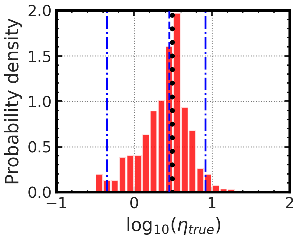
Figure 1: Data Distribution: The distribution of the viscosity ($\eta_{true}$) from the Vlugt data set Jamali et al. (2018b) across decades of viscosity. The blue vertical dashed line represents the median and the two blue vertical dash-dot lines represent the 95 percentile range around the median. The black dotted line represents the mean of the data.

III.1.1 Vlugt data set

Recently, Vlugt and co-workers simulated 250 binary Lennard-Jones fluids to study the system size dependence of the self-diffusion coefficients.Jamali et al. (2018b) In order to test the analytical expression for the system size corrections to the self-diffusion coefficients, they also computed the viscosity using the Einstein-Helfand equation.Allen and Tildesley (2017); Mondello and Grest (1997); Maginn et al. (2019) We found that their work reported the largest consistent data set that used multiple long independent runs to compute viscosity and crucially, its confidence interval. In view of these attributes, our ML models were built using this data set.

The data set contains a total of 1061 points, all of them at the same temperature and pressure of 0.65 and 0.05 respectively. All the quantities are reported in dimensionless units with interaction parameters of the first component as the base units i.e., $\sigma_{1}$ = 1, $\epsilon_{1}$ = 1 , mass₁ = 1. The state space is spanned by varying three interaction parameters ($\sigma_{2}$, $\epsilon_{2}$, k₁₂) and one compositional parameter (X₁). We call these parameters as ’pre-MD’ features to be consistent with ML nomenclature where the independent variables are called as features. Further, each state point was studied at four different system sizes (quantified in terms of the total number of particles in the simulation box). In sum, about 250 state points were simulated, each at four different system sizes, giving a total of about 1000 data points. Unlike the self diffusion coefficient, shear viscosity does not have a strong dependence on system size.Kim et al. (2018, 2019); Yeh and Hummer (2004); Tazi et al. (2012); Gabl, Schröder, and Steinhauser (2012); Jamali et al. (2018a); Wang et al. (2020); Petravic (2004) Hence, we use only the data points at the system size of 2000 particles (273 out of 1000 data points) to develop the ML models in this work.

In the raw data, viscosity values span four decades, from 10^-1 to 10³, but only two data points had a value greater than 20. These two data points ($\eta_{true}$ $>$ 20) were identified as outliers and were not considered during the ML modeling. Figure 1 shows the distribution of data points by their viscosity values indicating that most of the data points are populated around the mean viscosity value of around 3 and the extremal decades are sparsely populated. Due to the uneven distribution of viscosity values across decades, the models trained subsequently can be biased towards values around the mean. The distribution of the standard error relative to the corresponding mean is shown in Figure LABEL:sfig:viscerrdist. The relative standard error seems to be uncorrelated to the viscosity value itself indicating that the data across decades is of similar quality. The standard error on the mean was used to calculate the irreducible minimum value of various loss functions Bishop (2006) (also called as the Bayes error Goodfellow, Bengio, and Courville (2016)). The irreducible errors are incurred by all non-probabilistic ML models because of their approximation of the conditional density $\mathbb{E}_{y}[y|\mathrm{x}]$ by point estimates.Bishop (2006) The irreducible MSE is the average variance in the data. The irreducible MAE and MAPE were estimated by sampling from a Gaussian conditional density.Bishop (2006) We also note that, in general, metric value obtained from the average standard error would be different from the irreducible loss. For example, the MAPE value obtained from the average standard error(%) of the data is about 2%, whereas the irreducible MAPE is 0.8%. Unless explicitly mentioned, the metric values obtained from the average standard errors are used to compare the corresponding metrics from the ML models. Hence, we consider ML models with MAPE metric lower than 2 % to be successful models.

Furthermore, to get a preliminary understanding about the underlying correlations in the data, viscosity is plotted against other features - X₁, $\sigma_{2}$, $\epsilon_{2}$, k₁₂, box length, packing fraction ($\zeta$), and self-diffusion coefficients (D1 and D2). These features can be divided into two sets - preMD and postMD features. As their names suggest, the preMD feature set consists of all those features that are fixed before running the MD simulation and postMD features are obtained only after the MD simulations. In this case, there are four preMD features - X₁, $\sigma_{2}$, $\epsilon_{2}$, k₁₂ and six postMD features - number density, $\zeta$ and the four preMD features. As expected, self-diffusion coefficients are inversely correlated to viscosity, consistent with the Stokes-Einstein relation. Apart from self-diffusion constant, only the packing fraction seems to be well correlated with viscosity, with higher packing fractions corresponding to higher viscosity. Rest of the plots show a wide spread of viscosity values at any given feature value indicating that no single feature can predict viscosity accurately. See section LABEL:ssec:data-features for more details.

Two different sets of models, using postMD and preMD features respectively, were developed for each ML algorithm. Unless otherwise mentioned, the results presented are from the models developed using postMD features. All the features were scaled using Min-Max scaler before training the ML models. Also, the logarithm of viscosity was used as the label. However, all the metrics presented in the subsequent sections were computed on the untransformed viscosity values.

III.1.2 Interpolation data set

In order to test the predictive performance of the ML models away from the Vlugt data grid, a complementary data set called the interpolation data set was created. As the name suggests, the data set is created in the interpolation region of the preMD feature space of the Vlugt data set. The interpolation set consists of a total of 17 points at several interpolation distances. We note that the interpolation space is not entirely in the equilibrium liquid region of the binary LJ phase diagram at the thermodynamic conditions studied by Vlugt et al.Jamali et al. (2018b) Hence, it is difficult to generate a "representative sample" of the interpolation space, which is required to obtain quantitative estimates of predictive performance. In this context, the current data set of 17 points (though small) can be used to understand the predictive performance in a qualitative sense. Details of the MD simulation procedure used to create the interpolation data set are given in the Supporting Information.

III.1.3 Applicability Domain

Given that the interpolation space is not entirely in the liquid region, the ML models cannot be expected to perform well over the entire interpolation space, especially far away from the Vlugt data grid. One way to tackle this issue is to define an Applicability Domain (AD) within which the ML models are expected to perform well.Sheridan et al. (2004); Dimitrov et al. (2005); Schroeter et al. (2007); Fechner et al. (2010); Rakhimbekova et al. (2020) There are many methods to construct an AD and a detailed comparison is beyond the scope of this work.Schroeter et al. (2007); Fechner et al. (2010); Rakhimbekova et al. (2020) The Applicability Domain (AD) used in this work is described in section IV.3. The interpolation data set is divided into two parts called In-AD and Out-AD based on whether the points fall within or outside the AD respectively.

III.2 Machine Learning Models

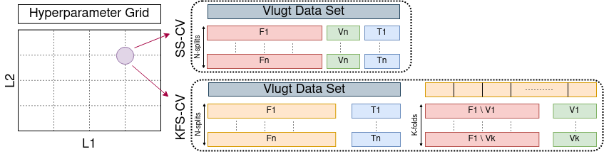
Figure 2: Model selection and performance estimation: A schematic representation of the two model selection procedures used in this study - Shuffle Split Cross validation (SS-CV) and K-fold Split Cross validation (KFS-CV). L1, L2 represent the hyperparameters to be tuned in the model selection procedure. F_i, V_i, T_i represent the train, validation and test sets respectively. See section LABEL:ssec:results-model-sel for more details.

A total of seven ML models were tested for their ability to predict shear viscosity - Kernel Ridge Regression (KRR), Artificial Neural Network (ANN), Gaussian Process Regression (GPR), Support Vector Regression (SVR), Random Forest (RF), k-Nearest Neighbors (KNN), and Least Absolute Shrinkage and Selection Operator (LASSO). In the current work, GPR is the probabilistic model (level 2 in section LABEL:ssec:struct) and all others are non-probabilistic in nature (level 2 in section LABEL:ssec:struct). Except ANN, all other the ML models used in this work were from the scikit-learn implementation.Pedregosa et al. (2011) The ANN models were built using the keras library in a python environment.Chollet et al. (2015) Many helper functions from numpy,Harris et al. (2020) scipy,Virtanen et al. (2020) pandas pandas development team (2020) and scikit-learn Pedregosa et al. (2011) were also used in the model construction, model selection and performance estimation steps.

III.3 Model Selection and Performance Estimation

In this work, we compare two popular model selection and performance estimation methods called - Shuffle Split Cross validation (SS-CV) and K-fold Split Cross validation (KFS-CV). A precise algorithmic description of these methods is given in section LABEL:ssec:comp-details-model-sel. Briefly, SS-CV splits the data set into three parts (named train/validation (val)/test) multiple times. Each time the data is shuffled and hence independent random realisations of the data can be obtained by SS-CV. KFS-CV is a two step procedure in which firstly entire data is split into two parts (named train/test) and later the train part is again split into k folds of roughly same size. The k folds (obtained in the second step) are used to obtain validation score and the test sets are used to do performance evaluation. Figure 2 summarizes the two procedures. Finally, we note that the procedures outlined above are referred to by slightly different names in the literature Beckner, Mao, and Pfaendtner (2018); Xu and Goodacre (2018); Bishop (2006); Cawley and Talbot (2010) and the ML software packages.Pedregosa et al. (2011) Hence we recommend using the algorithmic description of these methods given in section LABEL:ssec:comp-details-model-sel.

III.4 Interpolation Grid

The interpolation capabilities of the models can be qualitatively tested by plotting the predicted viscosity values at the grid of interpolated feature values. As the feature space is generally high dimensional (four in this case), only projections onto 1D/2D sub-spaces can be visualized. To keep the visualization uniform across the features, interpolation was done in the scaled feature space i.e., after the min-max scaler is applied. The Vlugt data set was generated at discrete values of each feature - X₁ : (0.1, 0.3, 0.5, 0.7, 0.9) , $\sigma_{2}$ : (1.0, 1.2, 1.4, 1.6), $\epsilon_{2}$ : (1.0, 0.8, 0.6, 0.5), k₁₂ : (0.05, 0.0, -0.3, -0.6). However, the final data set consists of only 250 unique combinations of preMD features as opposed to 320, had all the combinations been studied.

We have constructed four different interpolation grids to test the interpolation capability across each feature individually. The interpolation grid for a particular feature is generated at values uniformly spaced in the range of 0 to 1 while holding all other features at the values from the Vlugt data set. For example, in order to generate the X₁ interpolation grid, 19 uniformly distributed values between 0 to 1 were used for X₁, while the values for $\sigma_{2}$, $\epsilon_{2}$ and k₁₂ were taken from their scaled values in the Vlugt data set. We also define the interpolation distance of any interpolated point as its Euclidean distance from the nearest training data point.

IV Results and discussion

In this section, we first present evidence related to aspects of model selection and performance evaluation that are pertinent to ML models at the low data regime. We then compare different ML models based on their performance metrics and interpolation behavior. We finally compare the predicted uncertainties of ensemble models and that of a probabilistic ML model (GPR).

IV.1 Model Selection and Performance Estimation

IV.1.1 Understanding the Hyperparameter Optimization Landscapes

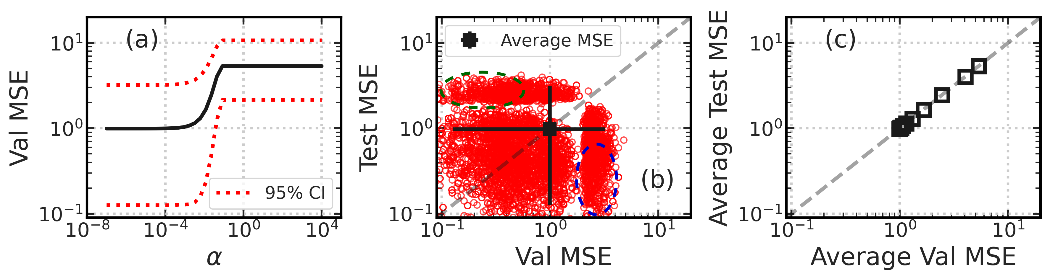
Figure 3: Model selection: (a) Average validation MSE plotted against the $\alpha$ hyperparameter of the LASSO model. The red dotted lines show the 95% confidence interval of the validation MSE. (b) A scatter plot of the individual test MSE and validation MSE at $\alpha=5*10^{-6}$. The black square shows the test MSE vs validation MSE averaged over the 5000 splits. The error bars correspond to the 95 percentile about the median of the respective MSE. The green and the blue ellipses are marked to indicate the data splits in which test MSE can be much greater or lower than validation MSE respectively. (c) Average test vs Average validation MSE at different values of the $\alpha$ hyperparameter of the LASSO model. The test and validation MSE were obtained using LASSO model and shuffle-split data sampling scheme (See Computational Methods).

In order to understand the optimization landscape of the hyperparameters, we use LASSO and KRR models. They were chosen because they have less than three hyperparameters and are hence conducive for the visualization of the optimization landscape in 2D plots. Moreover, both models have analytic solutions and are hence much faster when trained on small data sets. Both these models were also studied in the context of model selection (albeit on synthetic data sets) and hence allow a close comparison wherever possible.Cawley and Talbot (2010)

In this section, we elucidate the dependence of the performance of these ML models on the particulars of the data splitting procedure, which is an essential step for model selection and performance evaluation. The entire data set is randomly split into three parts - train, validation (val) and test sets with 60/20/20 ratio. This procedure is repeated $N_{split}$ times thereby creating multiple random realisations of the train, validation and test splits. These $N_{split}$ train sets are used to train $N_{split}$ ML models at each hyperparameter value. The trained models are then evaluated on their corresponding validation and test sets.

Figure 3 (a) shows the average test MSE of the LASSO model across a wide hyperparameter ($\alpha$) range. Clearly, $\alpha$ values less than $10^{-3}$ are suited for the viscosity data set. However, no single optimal hyperparameter can be selected as there is no discernible change in the MSE values for $\alpha$ less than $10^{-3}$. A similar "flat-minima" hyperparameter landscape was also observed by Pfaendtner et al. on an ionic liquid experimental viscosity data set.Beckner, Mao, and Pfaendtner (2018) Hence, strictly applying the common model selection criteria of selecting the hyperparameter with the best performance on the validation set (in this case, minimizing MSE) belies the flat-minima nature of hyperparameter landscape. Also, the wide confidence interval around the average test MSE indicates that there is significant variability in the performance (MSE) of the ML models across different data splits.

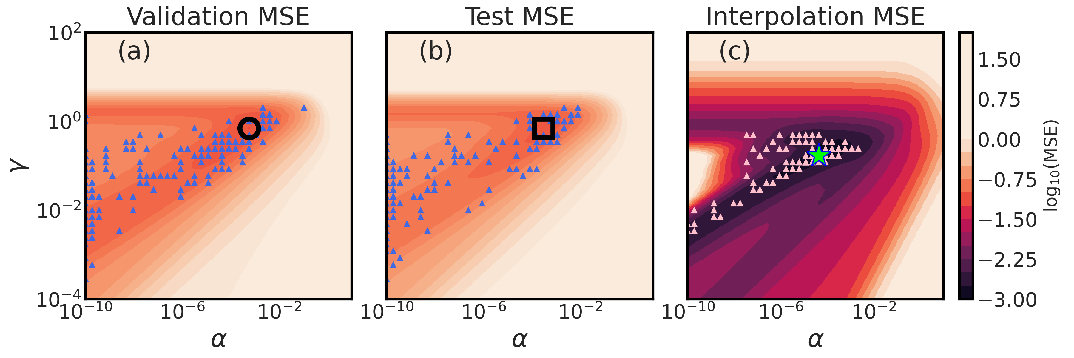
Figure 4: Model selection: 2D contour plots of (a) average validation MSE, (b) average test MSE and (c) Average Interpolation MSE of KRR model. The minima in the 2D contour plots are marked as follows - black-unfilled-circle: average validation MSE, black-unfilled-square: average test MSE, green-filled-star: average Interpolation MSE. The blue triangles in (a) and (b) mark the optimal hyperparameters that minimize individual validation and test MSE respectively. The pink triangles in (c) mark the optimal hyperparameters that minimize individual Interpolation MSE. The validation, test, and Interpolation MSE were obtained using KKR model and shuffle-split data sampling scheme (See Computational Methods).

Interestingly, the wide scatter of points in Figure 3 (b) indicates that the individual test MSEs are not correlated to individual validation MSEs. Hence model selection criteria based on optimization of the performance of individual validation sets need not necessarily result in a good generalization performance. However, the average validation MSE (over $N_{split}$ splits) is perfectly correlated to the average test MSE as shown in Figure 3 (c). Consequently, the data splitting procedures that reserve a single "unseen" data set (often called as test set Paduszyński and Domańska (2014); Allers et al. (2021)) for evaluating the generalization performance should be discouraged as they suffer from wide variability. We note that this problem is unique to small data sets and the variability decreases rapidly with increase in data set size.Cawley and Talbot (2010)

The same procedure was applied to the KRR model to elucidate its hyperparameter optimization landscape. In addition to validation and test sets, the performance of the KRR models was also evaluated on a single Interpolation set containing 17 data points. Figure 4 shows the 2D contour plots of the average validation, test and Interpolation MSE over a wide range of KRR hyperparameters $\alpha$ and $\gamma$. The landscapes of the average test and validation MSE are similar, consistent with the LASSO results (Figure 4). The Interpolation MSE landscape is slightly different from others near the minima while still retaining the overall features. Importantly, it is more rugged than the validation and test MSE landscapes, possibly because the same Interpolation set was used across all the $N_{split}$ splits.

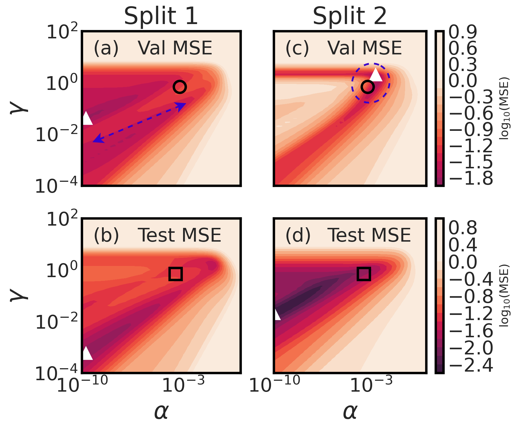
Figure 5: Model selection: (a) and (b) show 2D contour plots of the individual validation and test MSE respectively of a randomly chosen realisation (called split 1) of the train-val-test split. (c) and (d) show the same for another random realisation (called split 2) of the train-val-test split. In all panels, the minima of the average MSE are marked as follows: black-unfilled-circle: average validation MSE, black-unfilled-square: average test MSE. The minima of these particular realisations are marked with a white triangle symbol. The blue dashed arrow in (a) is drawn as a guide to the eye to highlight the large difference between the individual (white triangle) and the the average (black circle) minima. The blue dashed ellipse in (c) is drawn as a guide to the eye to indicate that the individual and the the average minima can be close by chance. The validation and test were obtained using KRR model and shuffle-split data sampling scheme (See Computational Methods).

The wide scatter of points in Figure 4 (a,b,c) show the optimal hyperparameter selected by minimizing the individual validation, test and Interpolation MSE respectively. This demonstrates that using a single realisation of data split to model selection or performance evaluation can result in wide variability, again consistent with LASSO results. Cawley et al. used KRR on a small synthetic data set to demonstrate this issue of wide variability when single realisations of data are used.Cawley and Talbot (2010) Further, while the average MSE landscapes are smooth, those corresponding to individual realisations of the data splits are rugged as shown in Figure 5. The validation and test landscapes of these individual splits also show significant differences. For example, Figure 5 (d-f) corresponds to validation, test and Interpolation landscapes of a randomly chosen realisation and their optimal hyperparameters vary by more than seven orders of magnitude.

These results demonstrate that there is a wide variability in choosing the optimal hyperparameter values (model selection) and also in estimating the generalization performance (performance evaluation) of the ML models on small data sets. Hence, it is crucial to do both the model selection and performance evaluation tasks by training an ensemble of models on different random splits of the data set.

IV.1.2 Comparison of CV Procedures

The model selection criterion is based on the average validation score obtained from the CV procedures. We observe that the average validation score landscapes are almost identical in both SS-CV and KFS-CV irrespective of the kind of metric used to construct the landscape (Figure LABEL:sfig:ss-vs-kfs-mean). However, the two procedures differ in the variance of the validation landscape, with KFS-CV yielding a lower variance than SS-CV (Figure LABEL:sfig:ss-vs-kfs-relerr). Cawley et al. show that the estimators with lower variance can do a better job of selecting the optimal hyperparameters.Cawley and Talbot (2010) Hence we use KFS-CV to do model selection and performance evaluation on rest of the ML models - SVR, RF, KNN, ANN.

Also, in both the CV procedures, the variance of the validation landscapes was strongly dependent on the error metric used to construct the landscapes. In general, we observe that MSE shows the highest variance followed by MAE, MAPE and R². The variance in MSE validation landscape is often so high ($>100\%$), that unambiguous selection of optimal hyperparameters is difficult. Hence, the use of other metrics that that have lesser variance such as MAE, MAPE, R² can help rectify the issue. In this work, we use the MAE validation landscape to choose the optimal hyperparameter values. Tables in section LABEL:ssec:results-hyperpar-sel list the optimal hyperparameters and the corresponding values of metrics for all the ML models studied in this work.

Finally, the performance estimation is done by evaluating the trained models (with the optimal hyperparameters) on the test sets. As both CV procedures result in nearly identical performance scores, we use the KFS-CV method to do the performance estimation for the other ML models - SVR, RF, KNN, ANN. In the following section, we compare the performance of various ML methods and rank them using multiple metrics.

IV.2 Model Comparison and Ranking

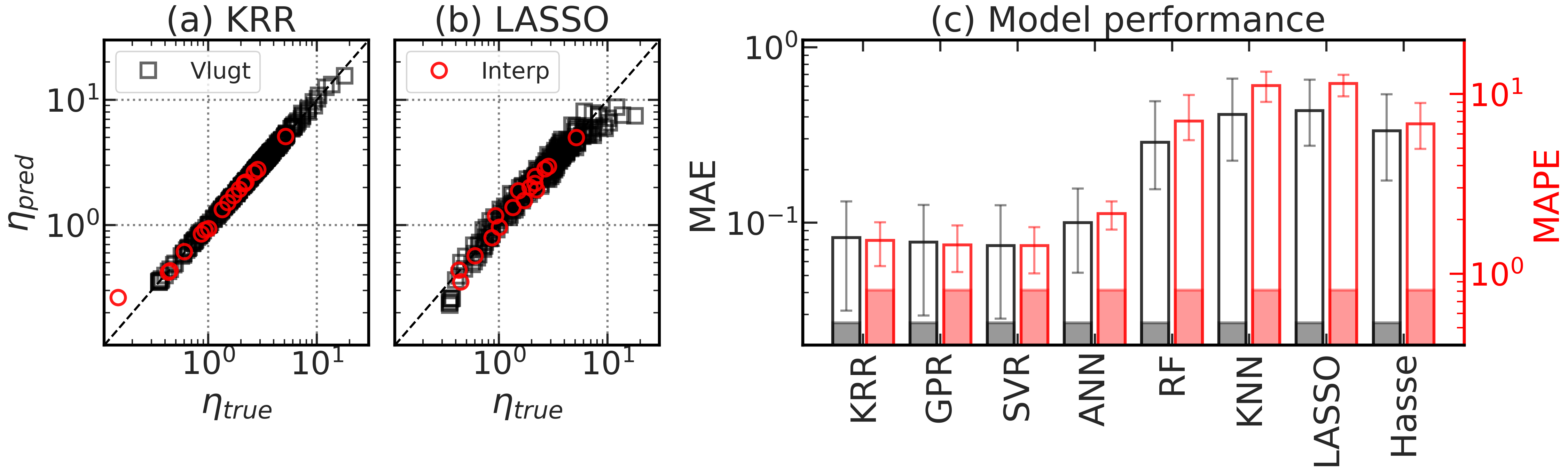
Figure 6: Model performance: (a),(b) Predicted vs the true viscosity values from KRR and LASSO ensemble models respectively. The black squares are for the Vlugt data set and the red circles are for the interpolation data generated in this work. The black dashed line represents the y=x line. (c) Comparison of the Mean Absolute Error (MAE) and Mean Absolute Percentage Error (MAPE) of all the seven ML models studied in this work. The performance of the empirical correlation by Hasse et al. Lautenschlaeger and Hasse (2019) is also shown for comparison. The black bars show the MAE and the red bars show the MAPE. The error bars indicate the 95% confidence interval region. The filled regions of the bars indicate the irreducible errors (0.027 for MAE and 0.8% for MAPE) in the Vlugt data set (section III.1.2). See the computational methods section for model description and performance estimation.

The predicted viscosity values from all the models, except KNN and LASSO, agree well with the true viscosity values both for test and interpolation data sets as shown in Figure 6. The agreement is seen to be good across decades of viscosity values indicating, at least to the naked eye (Figure 6 (a)), that models do not bias any particular decade of viscosity values. A detailed discussion on the model bias is presented in the Supporting Information (section LABEL:ssec:model-bias). Figure 6 (c) compares the MAE and MAPE of all the models evaluated using the KFS-CV performance estimation procedure (section III.3). The MAPE of KRR, GPR, ANN and SVR models are below the average standard error (%) of the data (called as threshold henceforth) and hence can be considered as successful models. On the other hand, KNN and LASSO models have both their test and train MAPE much above the threshold and can hence be considered as unsuccessful models. While the RF model performs well, it is still considered unsuccessful, due to its peculiar interpolation behavior (see discussion below). Also, the successful models outperform the empirical model developed by Hasse et al. for pure LJ fluids (see section LABEL:ssec:emp-model).Lautenschlaeger and Hasse (2019)

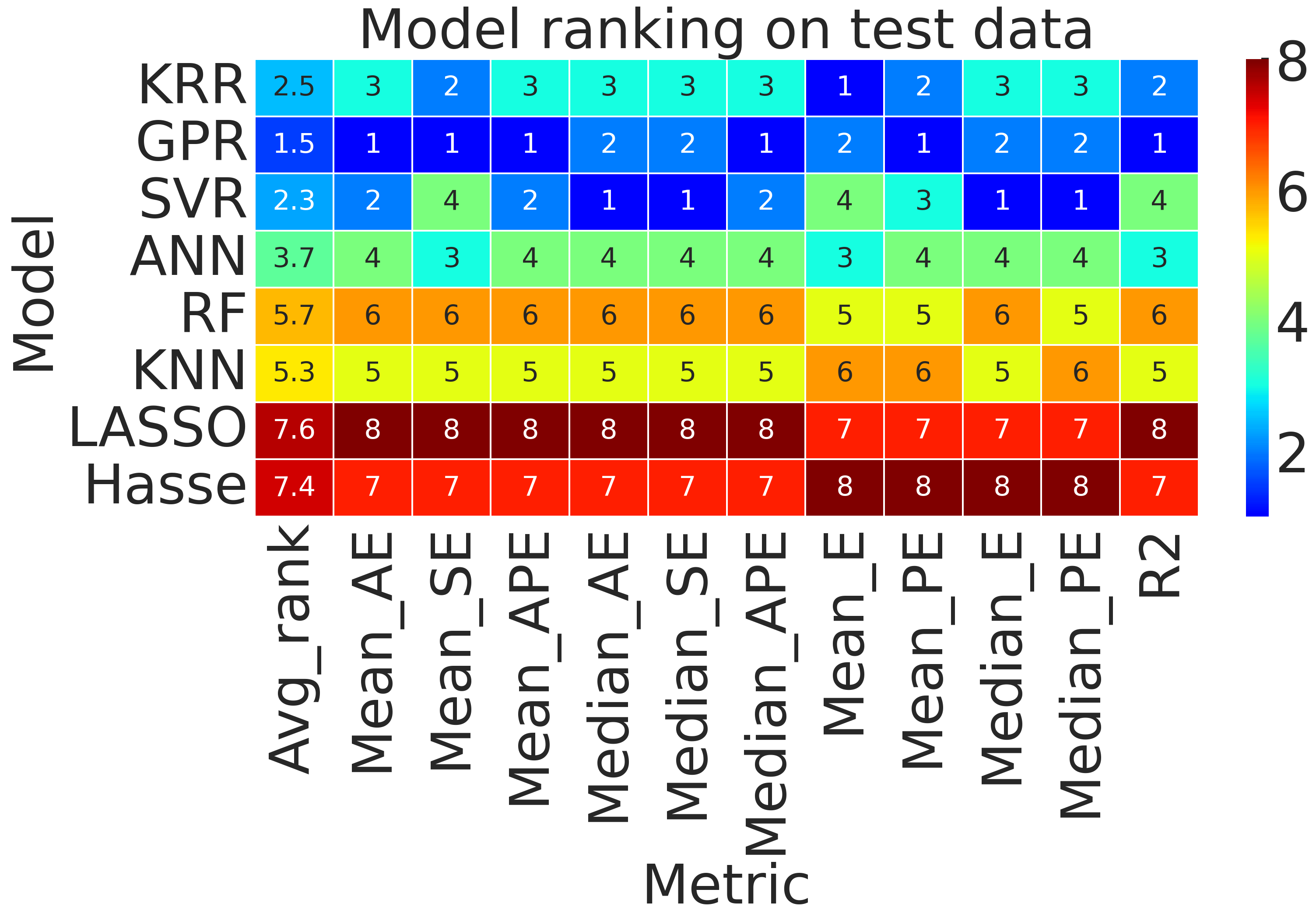
Figure 7: Model ranking: Grid plots of model’s ranking on the entire Vlugt data based on various metrics. The text and color of each square represent the relative ranks of models. Each row shows the ranks of the model labeled on the y-axis and each column corresponds to the metric based on which the ranking was done. The metric values are computed using the ensemble predictions of the ML models on the entire Vlugt data.Jamali et al. (2018b) Lower model rank is better.

The MAE and MAPE of the successful models - i.e., KRR, GPR, ANN, and SVR - are very close to each other as seen in Figure 6 (c) and hence more information is required to unambiguously rank them. In Figure 7, we show the relative ranks of all the models based on seven (MAE, MSE, MAPE, MedAE, MedSE, MedAPE and R²)performance based metrics and four (ME, MPE, MedE, MedPE) bias based metrics. The mean, median values of the Absolute Error (AE), Squared Error (SE), and the Absolute Percentage Error (APE) along with the coefficient of determination (R²) are the performance metrics, while mean, median Error (E) and the Percentage Error (PE) constitute the bias metrics. An average rank (averaging done across the metrics with uniform weights) is also shown for each model. The average rank follows closely the MAE rank with four successful models - KRR, GPR, SVR, and ANN - having an average rank less than four and three unsuccessful models having a rank greater than four. According to the average rank, GPR is the best performing model, followed closely by SVR and KRR. These three models are followed by ANN, RF, KNN, and LASSO respectively with the last two consistently ranked sixth and seventh. Interestingly, there is considerable mixing of ranks based on MAE vs MSE, indicating that a holistic approach using a combination of metrics needs to be used to objectively evaluate the models. Another noticeable trend is the disconnect between the ranking based on performance and those based on bias metrics. These findings highlight the need to evaluate models based on metrics beyond the simple loss functions used to train the models themselves to get a complete picture of the models accuracy, bias and generalizability. Now that the models have been validated for performance and bias, we discuss their interpolation capabilities in the next section.

IV.2.1 Interpolation Behaviour

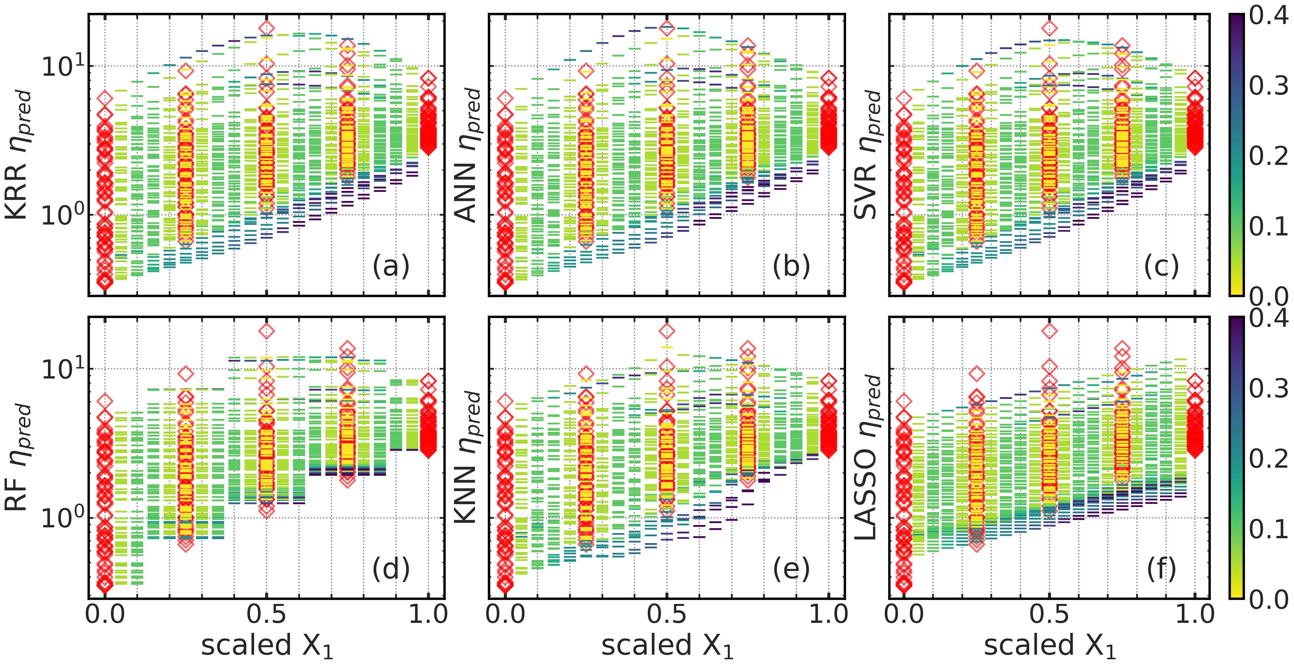
Figure 8: Model interpolation: (a) to (f) show the predicted viscosity values from the ensembles of KRR, ANN, SVR, RF, KNN, and LASSO respectively in the X₁ interpolation range. Red diamonds are viscosity values from the Vlugt data set. The color of the dashes indicate the distance from the nearest Vlugt data point in the scaled feature space (abscissa). See Computational Methods section for details on feature scaling and the construction of the interpolation grid.

Figure 8 shows the predicted viscosity values from KRR, ANN, SVR, RF, KNN, and LASSO models at the interpolation points plotted against X₁ feature values. The color of the points (represented as dashes in the figure) indicates the distance from the nearest training data point that the models have seen, with darker shades being farther away. The viscosity values from the Vlugt data set are also shown (as red diamond symbols) for comparison. KRR, SVR, and ANN models show a smooth variation as the feature values move farther away from their corresponding values in the Vlugt data set. On the other hand, RF and KNN models show sudden discontinuities in the predicted viscosity values at some specific X₁ values. These discontinuities are probably due to the presence of decision boundaries in RF and a sudden change of nearest neighbors in the case of KNN. Such sudden discontinuities are incompatible with viscosity which is expected to be continuous (at least as long as there is no phase transition).

IV.3 Uncertainty Quantification

As demonstrated in the previous sections, the performance of ML models trained on small data sets can have wide variations. In this regard, models that can estimate the uncertainty on individual predictions can help alleviate this issue. The uncertainty estimates can be used as a guide to end-users about the reliability of a given prediction and thus of the models. More generally, uncertainty quantification has many other applications Schwaighofer et al. (2007); Peterson, Christensen, and Khorshidi (2017); Tavazza, DeCost, and Choudhary (2021); Scalia et al. (2020); Imbalzano et al. (2021) such as - setting the applicability domain of the ML models,Schroeter et al. (2007) active learning for generating data on the fly,Vandermause et al. (2020); Xie et al. (2022) etc.

Figure 9: Uncertainty Comparison: The standard errors of the predicted viscosity values plotted against their corresponding true standard errors. The standard errors from the ensemble of KRR models are shown as black circles and those from the GPR model are shown as red squares. The grey dashed line corresponds to y=x and is drawn as a guide to the eye.

In this work, we used two approaches to estimate the uncertainty - probabilistic ML method and ensemble ML method. The probabilistic ML methods inherently capture the uncertainty through their model architecture, whereas the ensemble ML approach uses an ensemble of ML models on several random realisations of the data. Gaussian Process Regression (GPR) was the choice of probabilistic ML method due to its simplicity (few hyperparameters), wide applicability and near universality. KRR was used to test the ensemble approach again due to its simplicity (two hyperparameters), training speed (analytical solution) and wide applicability.

Figure 9 compares the standard error estimated from the ML models and the true standard error of the data. Both GPR and ensemble KRR methods show good agreement with the true data. The standard errors predicted by GPR show a slightly better agreement with that of the data than KRR ensemble does, especially at high error values. This is because the ensemble methods capture the uncertainty in the data indirectly by repeated sampling from the training data set. On the other hand, the standard error values of the data are directly fed into the GPR training. A similar observation was made by M$\ddot{\rm u}$ller et al. on their comparison of GPR and ensemble methods to predict error bars on the solubility data.Schroeter et al. (2007)

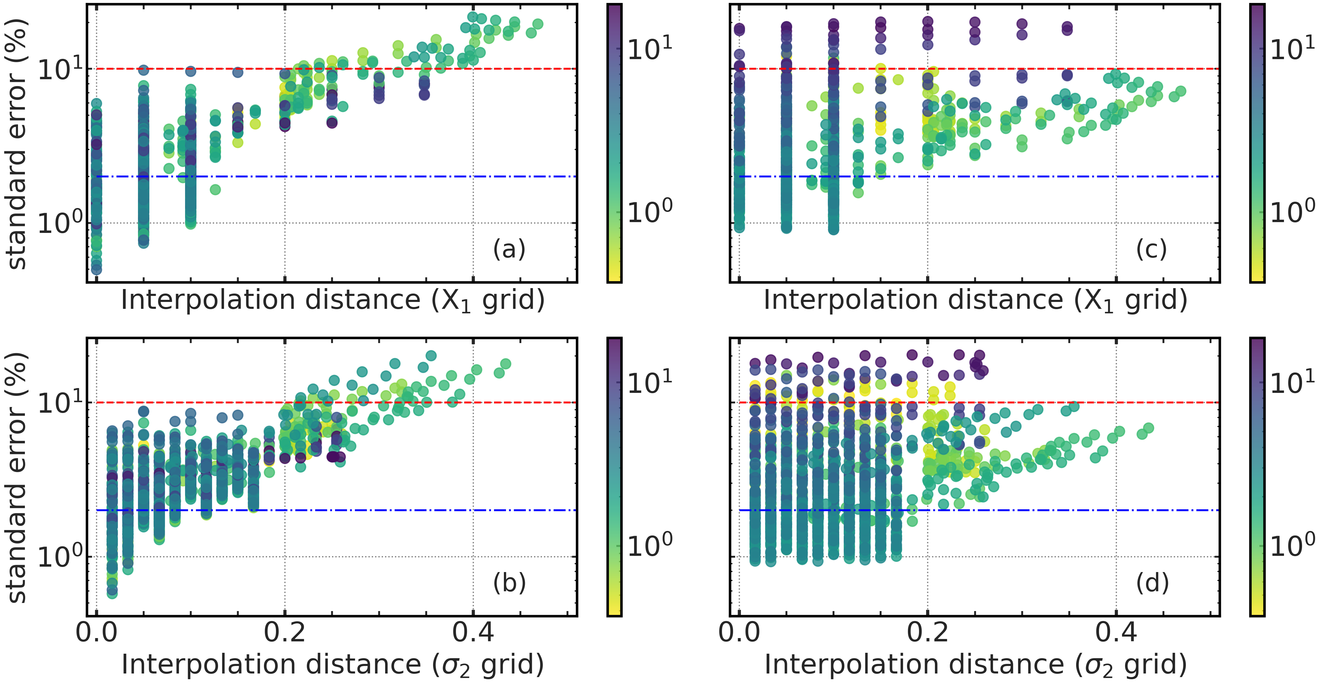
Figure 10: Interpolation Uncertainty: (a), (b) show the GPR predicted relative standard error (%) plotted against the interpolation distance in the X₁, $\sigma_{2}$ interpolation grids respectively. (c), (d) show the KRR ensemble predicted relative standard error (%) plotted against the interpolation distance in the X₁, $\sigma_{2}$ interpolation grids respectively. The colors indicate the predicted mean viscosity value corresponding to the interpolation point. The blue horizontal dash-dot line indicates the average standard error(%) (2%) of the Vlugt data set and the red horizontal dashed line indicates 10% standard error(%) which is then used to define a qualitative cut-off for the Applicability Domain. The interpolation distance is computed in the scaled feature space.

Information about closeness of a new query point to the training data would be useful to decide whether or not to trust the values predicted by the model. This information can be naturally encoded into GPR in the form of epistemic uncertainty.Vandermause et al. (2020) Ideally, the predicted standard error should increase beyond the natural uncertainty in the data as the query point moves away from the training data set. Figure 10 (a),(b) show the predicted relative standard error from the GPR model plotted against the interpolation distance with the colors indicating the predicted mean viscosity value. The predicted relative standard errors clearly increase with increasing interpolation distance. However, this behavior could not be seen in the case of relative standard errors estimated by the ensemble method as seen in Figure 10 (c),(d). Hence, the uncertainties estimated by GPR represent the true uncertainties better and also systematically increase when the query points move far from the training set. Additionally, GPR needs to be trained only once when compared to ensemble methods which need to be trained over multiple realisations of the training set.

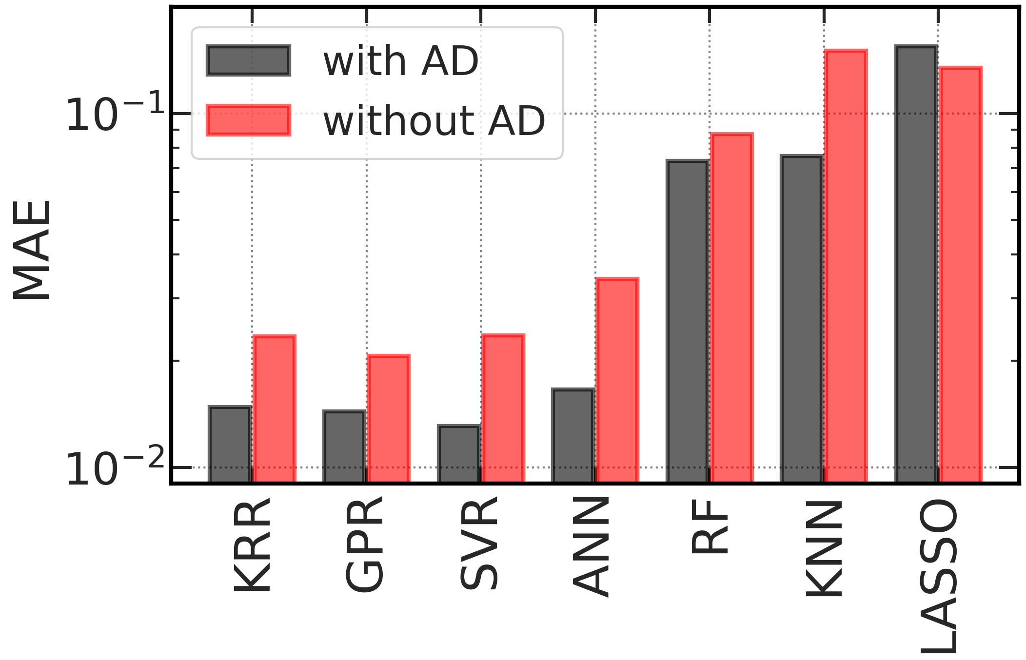
Figure 11: Applicability Domain (AD): MAE values of the ensemble ML models estimated on the interpolation data set. The red bars indicate the MAE values on the entire interpolation data (without Applicability Domain) and the black bars indicate the MAE values on the part of the interpolation data that falls within the Applicability Domain (In-AD). Due to the small size of interpolation data set, these MAE values should be compared in a qualitative sense.

Finally, the standard errors predicted by the GPR can be used to construct applicability domain of the ML models.Schroeter et al. (2007) For example, for queries which have a distance less than 0.2 (in the scaled feature space) from the nearest training point, a relative error of less than 10% can be expected (Figure 10). Hence, the scaled distance of 0.2 can be set as a limit for the Applicability Domain, beyond which the predictions from the ML models need to be treated with caution. Though such a distance based approach is simple, it can be applied to any ML model thereby justifying its use.Schroeter et al. (2007) Also, such distance based AD methods have been successfully implemented for QSAR Sheridan et al. (2004) and ML models.Schroeter et al. (2007)

The interpolation data set was split into In-AD and Out-AD based on whether the points fell within the AD or otherwise. The performance of all the ML models on the In-AD data set is much better than that on Out-AD set, demonstrating that the application of AD can be used to detect and remove the outliers (Figure 11). Also, the improvements from the AD (though constructed from GPR only) were observed across all the ML models and performance metrics.

V Conclusions

In this work, we trained and evaluated several successful ML models to predict the shear viscosity of binary LJ fluids. Being a collective property, shear viscosity is expensive to predict from equilibrium atomistic MD simulations and hence only small data sets can be found in the literature. The major challenges posed by the small data sets on ML methods are discussed. Specifically, we focus on - 1. model selection and performance estimation, 2. performance metrics, and 3. uncertainty quantification.

ML models are prone to overfitting on small data sets at both the model parameters and hyperparameter levels. We discuss various model selection methods - K-fold CV, nested K-fold CV, Monte Carlo CV, etc. - that are generally used to address this issue. While these methods are commonly used for selecting hyperparameters, the generalization error (performance evaluation) is estimated on a single unseen data set (test set). We demonstrate that such estimates are prone to wide variability because of the small data set size. The hyperparameter optimization landscapes of LASSO, KRR models are shown to have "flat-minima" thereby making it difficult to unambiguously select the optimal hyperparameters. We compared two simple CV procedures - SS-CV and KFS-CV and found that while their mean error estimates were almost identical, KFS-CV showed lower variance. Hence, it was chosen to both the model selection and performance estimation tasks simultaneously.

We discuss the role of performance metrics in model training and model evaluation, both from theoretical and empirical standpoints. We compare several commonly used metrics like MSE, MAE, MAPE and R² and discuss their relevance to the viscosity data set. We propose a holistic model ranking procedure based on inputs from multiple complementary metrics. The interpolation behavior of the ML models are compared qualitatively. While the KRR, ANN and SVR models showed smooth interpolation behavior, RF and KNN models showed sudden discontinuities and are hence considered unsuccessful. The successful models are also shown to outperform the best-in-class empirical model of Hasse et al.Lautenschlaeger and Hasse (2019)

We present two methods to estimate uncertainty in individual predictions from the ML models - 1. Gaussian Process Regression (GPR) and 2. ensemble of KRR ML models. The uncertainty (in terms of standard error) estimated by the methods showed overall agreement with the the true uncertainty of the data, with GPR faring slightly better. The behavior of the estimated uncertainty by both the methods in the interpolation feature range is also compared. The GPR’s uncertainty steadily increased as the query data points moved away from the training data, while no discernible pattern could be identified in the uncertainty from the ensemble method. The relative standard error estimated from the GPR model can be used to set distance limits for the query points thereby defining the applicability domain (AD) in which the results from the ML models are reliable. We found that the points of the interpolation set that fell within the AD were better estimated by the ML models than the ones that fell outside the AD, thereby demonstrating the utility of AD. Finally, the principles discussed in this work can be applied to develop ML models of viscosity for more complex fluids. However, in such fluids, the identification of the features that are most relevant to shear viscosity would also be non-trivial and constitutes a part of our future work.

Supplementary Information

See the Supplementary Information for additional information on theoretical background, model description, Vlugt data set, empirical model description, computational details of model selection, model performance, bias, etc.

AUTHOR DECLARATIONS

Conflict of Interest

The authors have no conflicts to disclose.

Author Contributions

Nikhil V. S. Avula Formal Analysis (lead); Methodology (lead); Software (lead); Visualization (lead); Writing/Original Draft Preparation (lead); Writing/Review & Editing (equal); Validation (equal); Data Curation (equal); Conceptualization (supporting); Funding Acquisition (supporting); Shivanand K. Veesam Data Curation (equal); Software (supporting); Validation (equal); Sudarshan Behera Formal Analysis (supporting); Methodology (supporting); Software (supporting); Writing/Review & Editing (supporting); Sundaram Balasubramanian Conceptualization (lead); Funding Acquisition (lead); Project Administration (lead); Resources (lead); Supervision (lead); Writing/Review & Editing (equal);

Data Availability Statement

The data that supports the findings of this study are available within the article and its supplementary material.

Appendix A Performance Metrics

$$e_{i}=y_{i}^{pred}-y_{i}^{true}$$ (4)

$$r_{i}=(y_{i}^{pred}-y_{i}^{true})/y_{i}^{true}$$ (5)

$$\bar{y}=\frac{1}{N}\sum_{i=1}^{N}y_{i}^{true}$$ (6)

$$ME=\frac{1}{N}\sum_{i=1}^{N}e_{i}$$ (7)

$$MPE=\frac{1}{N}\sum_{i=1}^{N}100\times\,r_{i}$$ (8)

$$MSE=\frac{1}{N}\sum_{i=1}^{N}e_{i}^{2}$$ (9)

$$MedSE=median({e_{i}^{2}})$$ (10)

$$MAE=\frac{1}{N}\sum_{i=1}^{N}|e_{i}|$$ (11)

$$MedAE=median({|e_{i}|})$$ (12)

$$MAPE=\frac{1}{N}\sum_{i=1}^{N}100\times\,|r_{i}|$$ (13)

$$MedAPE=100\times\,median({|r_{i}|})$$ (14)

$$R^{2}=1-\sum_{i=1}^{N}\frac{|e_{i}|^{2}}{|y_{i}^{true}-\bar{y}|^{2}}$$ (15)

References

- March and Tosi (2002) N. March and M. Tosi, Introduction to Liquid State Physics (World Scientific, 2002).
- Levashov, Morris, and Egami (2011) V. A. Levashov, J. R. Morris, and T. Egami, “Viscosity, shear waves, and atomic-level stress-stress correlations,” Phys. Rev. Lett. 106, 115703 (2011).
- Giordano, Russell, and Dingwell (2008) D. Giordano, J. K. Russell, and D. B. Dingwell, “Viscosity of magmatic liquids: A model,” Earth and Planetary Science Letters 271, 123–134 (2008).
- de Wijs et al. (1998) G. A. de Wijs, G. Kresse, L. Vočadlo, D. Dobson, D. Alfè, M. J. Gillan, and G. D. Price, “The viscosity of liquid iron at the physical conditions of the earth’s core,” Nature 392, 805–807 (1998).
- Vočadlo (2007) L. Vočadlo, “2.05 - mineralogy of the earth – the earth’s core: Iron and iron alloys,” in Treatise on Geophysics, edited by G. Schubert (Elsevier, Amsterdam, 2007) pp. 91–120.
- Secco (1995) R. A. Secco, “Viscosity of the outer core,” in Mineral Physics & Crystallography (American Geophysical Union (AGU), 1995) pp. 218–226, https://agupubs.onlinelibrary.wiley.com/doi/pdf/10.1029/RF002p0218 .
- Baled et al. (2018) H. O. Baled, I. K. Gamwo, R. M. Enick, and M. A. McHugh, “Viscosity models for pure hydrocarbons at extreme conditions: A review and comparative study,” Fuel 218, 89–111 (2018).
- Kontogeorgis et al. (2021) G. M. Kontogeorgis, R. Dohrn, I. G. Economou, J.-C. de Hemptinne, A. ten Kate, S. Kuitunen, M. Mooijer, L. F. Žilnik, and V. Vesovic, “Industrial requirements for thermodynamic and transport properties: 2020,” Industrial & Engineering Chemistry Research 60, 4987–5013 (2021).
- Maginn et al. (2019) E. J. Maginn, R. A. Messerly, D. J. Carlson, D. R. Roe, and J. R. Elliott, “Best practices for computing transport properties 1. self-diffusivity and viscosity from equilibrium molecular dynamics,” Living J. Comp. Mol. Sci. 1, 6324 (2019).
- Hess (2002) B. Hess, “Determining the shear viscosity of model liquids from molecular dynamics simulations,” The Journal of Chemical Physics 116, 209–217 (2002).
- Alfè and Gillan (1998) D. Alfè and M. J. Gillan, “First-principles calculation of transport coefficients,” Phys. Rev. Lett. 81, 5161–5164 (1998).
- Jamali et al. (2018a) S. H. Jamali, R. Hartkamp, C. Bardas, J. Söhl, T. J. H. Vlugt, and O. A. Moultos, “Shear viscosity computed from the finite-size effects of self-diffusivity in equilibrium molecular dynamics,” Journal of Chemical Theory and Computation 14, 5959–5968 (2018a).
- Li et al. (2021) Q. Li, T. Sun, Y.-g. Zhang, J.-W. Xian, and L. Vočadlo, “Atomic transport properties of liquid iron at conditions of planetary cores,” The Journal of Chemical Physics 155, 194505 (2021).
- Malosso et al. (2022) C. Malosso, L. Zhang, R. Car, S. Baroni, and D. Tisi, “Viscosity in water from first-principles and deep-neural-network simulations,” npj Computational Materials 8, 139 (2022).
- Tazi et al. (2012) S. Tazi, A. Boţan, M. Salanne, V. Marry, P. Turq, and B. Rotenberg, “Diffusion coefficient and shear viscosity of rigid water models,” Journal of Physics: Condensed Matter 24, 284117 (2012).
- Wang et al. (2020) H. Wang, R. S. DeFever, Y. Zhang, F. Wu, S. Roy, V. S. Bryantsev, C. J. Margulis, and E. J. Maginn, “Comparison of fixed charge and polarizable models for predicting the structural, thermodynamic, and transport properties of molten alkali chlorides,” The Journal of Chemical Physics 153, 214502 (2020).
- Fedosov et al. (2011) D. A. Fedosov, W. Pan, B. Caswell, G. Gompper, and G. E. Karniadakis, “Predicting human blood viscosity in silico,” Proceedings of the National Academy of Sciences 108, 11772–11777 (2011).
- Zhang, Otani, and Maginn (2015) Y. Zhang, A. Otani, and E. J. Maginn, “Reliable viscosity calculation from equilibrium molecular dynamics simulations: A time decomposition method,” Journal of Chemical Theory and Computation 11, 3537–3546 (2015).
- Müller-Plathe (1999) F. Müller-Plathe, “Reversing the perturbation in nonequilibrium molecular dynamics: An easy way to calculate the shear viscosity of fluids,” Phys. Rev. E 59, 4894–4898 (1999).
- Ewen, Heyes, and Dini (2018) J. P. Ewen, D. M. Heyes, and D. Dini, “Advances in nonequilibrium molecular dynamics simulations of lubricants and additives,” Friction 6, 349–386 (2018).
- Heyes, Dini, and Smith (2018) D. M. Heyes, D. Dini, and E. R. Smith, “Incremental viscosity by non-equilibrium molecular dynamics and the eyring model,” The Journal of Chemical Physics 148, 194506 (2018).
- Stillinger and Debenedetti (2005) F. H. Stillinger and P. G. Debenedetti, “Alternative view of self-diffusion and shear viscosity,” The Journal of Physical Chemistry B 109, 6604–6609 (2005).
- Jones and Mandadapu (2012) R. E. Jones and K. K. Mandadapu, “Adaptive green-kubo estimates of transport coefficients from molecular dynamics based on robust error analysis,” The Journal of Chemical Physics 136, 154102 (2012).
- Kim, Borodin, and Karniadakis (2015) C. Kim, O. Borodin, and G. E. Karniadakis, “Quantification of sampling uncertainty for molecular dynamics simulation: Time-dependent diffusion coefficient in simple fluids,” Journal of Computational Physics 302, 485–508 (2015).
- Oliveira and Greaney (2017) L. d. S. Oliveira and P. A. Greaney, “Method to manage integration error in the green-kubo method,” Phys. Rev. E 95, 023308 (2017).
- Heyes, Smith, and Dini (2019) D. M. Heyes, E. R. Smith, and D. Dini, “Shear stress relaxation and diffusion in simple liquids by molecular dynamics simulations: Analytic expressions and paths to viscosity,” The Journal of Chemical Physics 150, 174504 (2019).
- Heyes, Dini, and Smith (2020) D. M. Heyes, D. Dini, and E. R. Smith, “Single trajectory transport coefficients and the energy landscape by molecular dynamics simulations,” The Journal of Chemical Physics 152, 194504 (2020).
- Heyes, Dini, and Smith (2021) D. M. Heyes, D. Dini, and E. R. Smith, “Viscuit and the fluctuation theorem investigation of shear viscosity by molecular dynamics simulations: The information and the noise,” The Journal of Chemical Physics 154, 074503 (2021).
- Heyes and Dini (2022) D. M. Heyes and D. Dini, “Intrinsic viscuit probability distribution functions for transport coefficients of liquids and solids,” The Journal of Chemical Physics 156, 124501 (2022).
- Avula et al. (2021) N. V. S. Avula, A. Karmakar, R. Kumar, and S. Balasubramanian, “Efficient parametrization of force field for the quantitative prediction of the physical properties of ionic liquid electrolytes,” Journal of Chemical Theory and Computation 17, 4274–4290 (2021).
- Kondratyuk and Pisarev (2021) N. D. Kondratyuk and V. V. Pisarev, “Predicting shear viscosity of 1,1-diphenylethane at high pressures by molecular dynamics methods,” Fluid Phase Equilibria 544-545, 113100 (2021).
- Goloviznina et al. (2021) K. Goloviznina, Z. Gong, M. F. Costa Gomes, and A. A. H. Pádua, “Extension of the cl&pol polarizable force field to electrolytes, protic ionic liquids, and deep eutectic solvents,” Journal of Chemical Theory and Computation 17, 1606–1617 (2021).
- Gong and Sun (2019) Z. Gong and H. Sun, “Extension of team force-field database to ionic liquids,” Journal of Chemical & Engineering Data 64, 3718–3730 (2019).
- Kim et al. (2018) K.-S. Kim, M. H. Han, C. Kim, Z. Li, G. E. Karniadakis, and E. K. Lee, “Nature of intrinsic uncertainties in equilibrium molecular dynamics estimation of shear viscosity for simple and complex fluids,” The Journal of Chemical Physics 149, 044510 (2018).
- Wang, Lamim Ribeiro, and Tiwary (2020) Y. Wang, J. M. Lamim Ribeiro, and P. Tiwary, “Machine learning approaches for analyzing and enhancing molecular dynamics simulations,” Current Opinion in Structural Biology 61, 139–145 (2020), theory and Simulation, Macromolecular Assemblies.
- Noé et al. (2020) F. Noé, A. Tkatchenko, K.-R. Müller, and C. Clementi, “Machine learning for molecular simulation,” Annual Review of Physical Chemistry 71, 361–390 (2020).
- Karthikeyan and Priyakumar (2021) A. Karthikeyan and U. D. Priyakumar, “Artificial intelligence: machine learning for chemical sciences,” Journal of Chemical Sciences 134, 2 (2021).
- Bonati, Piccini, and Parrinello (2021) L. Bonati, G. Piccini, and M. Parrinello, “Deep learning the slow modes for rare events sampling,” Proceedings of the National Academy of Sciences 118, e2113533118 (2021), https://www.pnas.org/doi/pdf/10.1073/pnas.2113533118 .
- Doerr et al. (2021) S. Doerr, M. Majewski, A. Pérez, A. Krämer, C. Clementi, F. Noe, T. Giorgino, and G. De Fabritiis, “Torchmd: A deep learning framework for molecular simulations,” Journal of Chemical Theory and Computation 17, 2355–2363 (2021).
- Allers et al. (2020) J. P. Allers, J. A. Harvey, F. H. Garzon, and T. M. Alam, “Machine learning prediction of self-diffusion in lennard-jones fluids,” The Journal of Chemical Physics 153, 034102 (2020).
- Leverant, Harvey, and Alam (2020) C. J. Leverant, J. A. Harvey, and T. M. Alam, “Machine learning-based upscaling of finite-size molecular dynamics diffusion simulations for binary fluids,” The Journal of Physical Chemistry Letters 11, 10375–10381 (2020).
- Beckner, Mao, and Pfaendtner (2018) W. Beckner, C. M. Mao, and J. Pfaendtner, “Statistical models are able to predict ionic liquid viscosity across a wide range of chemical functionalities and experimental conditions,” Mol. Syst. Des. Eng. 3, 253–263 (2018).
- Koutsoukos et al. (2021) S. Koutsoukos, F. Philippi, F. Malaret, and T. Welton, “A review on machine learning algorithms for the ionic liquid chemical space,” Chem. Sci. 12, 6820–6843 (2021).
- Valderrama, Muñoz, and Rojas (2011) J. O. Valderrama, J. M. Muñoz, and R. E. Rojas, “Viscosity of ionic liquids using the concept of mass connectivity and artificial neural networks,” Korean Journal of Chemical Engineering 28, 1451–1457 (2011).
- Dutt, Ravikumar, and Rani (2013) N. V. K. Dutt, Y. V. L. Ravikumar, and K. Y. Rani, “Representation of ionic liquid viscosity-temperature data by generalized correlations and an artificial neural network (ann) model,” Chemical Engineering Communications 200, 1600–1622 (2013).
- Paduszyński and Domańska (2014) K. Paduszyński and U. Domańska, “Viscosity of ionic liquids: An extensive database and a new group contribution model based on a feed-forward artificial neural network,” Journal of Chemical Information and Modeling 54, 1311–1324 (2014).
- Fatehi, Raeissi, and Mowla (2017) M.-R. Fatehi, S. Raeissi, and D. Mowla, “Estimation of viscosities of pure ionic liquids using an artificial neural network based on only structural characteristics,” Journal of Molecular Liquids 227, 309–317 (2017).
- Baghban, Kardani, and Habibzadeh (2017) A. Baghban, M. N. Kardani, and S. Habibzadeh, “Prediction viscosity of ionic liquids using a hybrid lssvm and group contribution method,” Journal of Molecular Liquids 236, 452–464 (2017).
- Datta, Ramprasad, and Venkatram (2022) R. Datta, R. Ramprasad, and S. Venkatram, “Conductivity prediction model for ionic liquids using machine learning,” The Journal of Chemical Physics 156, 214505 (2022).
- Duong et al. (2022) D. V. Duong, H.-V. Tran, S. K. Pathirannahalage, S. J. Brown, M. Hassett, D. Yalcin, N. Meftahi, A. J. Christofferson, T. L. Greaves, and T. C. Le, “Machine learning investigation of viscosity and ionic conductivity of protic ionic liquids in water mixtures,” The Journal of Chemical Physics 156, 154503 (2022).
- Vishwakarma, Sonpal, and Hachmann (2021) G. Vishwakarma, A. Sonpal, and J. Hachmann, “Metrics for benchmarking and uncertainty quantification: Quality, applicability, and best practices for machine learning in chemistry,” Trends in Chemistry 3, 146–156 (2021), special Issue: Machine Learning for Molecules and Materials.
- Bishop (2006) C. M. Bishop, Pattern recognition and machine learning (New York : Springer, 2006).
- Goodfellow, Bengio, and Courville (2016) I. Goodfellow, Y. Bengio, and A. Courville, Deep Learning (MIT Press, 2016) http://www.deeplearningbook.org.
- Arlot and Celisse (2010) S. Arlot and A. Celisse, “A survey of cross-validation procedures for model selection,” Statistics Surveys 4, 40 – 79 (2010).
- Cawley and Talbot (2010) G. C. Cawley and N. L. C. Talbot, “On over-fitting in model selection and subsequent selection bias in performance evaluation,” Journal of Machine Learning Research 11, 2079–2107 (2010).
- Zhang and Yang (2015) Y. Zhang and Y. Yang, “Cross-validation for selecting a model selection procedure,” Journal of Econometrics 187, 95–112 (2015).
- Burnham and Anderson (2003) K. Burnham and D. Anderson, Model Selection and Multimodel Inference: A Practical Information-Theoretic Approach (Springer New York, 2003).
- Xu and Goodacre (2018) Y. Xu and R. Goodacre, “On splitting training and validation set: A comparative study of cross-validation, bootstrap and systematic sampling for estimating the generalization performance of supervised learning,” Journal of Analysis and Testing 2, 249–262 (2018).
- Armstrong and Collopy (1992) J. Armstrong and F. Collopy, “Error measures for generalizing about forecasting methods: Empirical comparisons,” International Journal of Forecasting 8, 69–80 (1992).
- Gneiting (2011) T. Gneiting, “Making and evaluating point forecasts,” Journal of the American Statistical Association 106, 746–762 (2011).
- Schwaighofer et al. (2007) A. Schwaighofer, T. Schroeter, S. Mika, J. Laub, A. ter Laak, D. Sülzle, U. Ganzer, N. Heinrich, and K.-R. Müller, “Accurate solubility prediction with error bars for electrolytes: A machine learning approach,” Journal of Chemical Information and Modeling 47, 407–424 (2007).
- Tran et al. (2020) K. Tran, W. Neiswanger, J. Yoon, Q. Zhang, E. Xing, and Z. W. Ulissi, “Methods for comparing uncertainty quantifications for material property predictions,” Machine Learning: Science and Technology 1, 025006 (2020).
- Scalia et al. (2020) G. Scalia, C. A. Grambow, B. Pernici, Y.-P. Li, and W. H. Green, “Evaluating scalable uncertainty estimation methods for deep learning-based molecular property prediction,” Journal of Chemical Information and Modeling 60, 2697–2717 (2020).
- Imbalzano et al. (2021) G. Imbalzano, Y. Zhuang, V. Kapil, K. Rossi, E. A. Engel, F. Grasselli, and M. Ceriotti, “Uncertainty estimation for molecular dynamics and sampling,” The Journal of Chemical Physics 154, 074102 (2021).
- Tavazza, DeCost, and Choudhary (2021) F. Tavazza, B. DeCost, and K. Choudhary, “Uncertainty prediction for machine learning models of material properties,” ACS Omega 6, 32431–32440 (2021).
- Kolassa (2020) S. Kolassa, “Why the “best” point forecast depends on the error or accuracy measure,” International Journal of Forecasting 36, 208–211 (2020), m4 Competition.
- Makridakis, Spiliotis, and Assimakopoulos (2020) S. Makridakis, E. Spiliotis, and V. Assimakopoulos, “The m4 competition: 100,000 time series and 61 forecasting methods,” International Journal of Forecasting 36, 54–74 (2020), m4 Competition.
- Hirschfeld et al. (2020) L. Hirschfeld, K. Swanson, K. Yang, R. Barzilay, and C. W. Coley, “Uncertainty quantification using neural networks for molecular property prediction,” Journal of Chemical Information and Modeling 60, 3770–3780 (2020).
- Wolpert and Macready (1997) D. Wolpert and W. Macready, “No free lunch theorems for optimization,” IEEE Transactions on Evolutionary Computation 1, 67–82 (1997).
- Hansen et al. (2013) K. Hansen, G. Montavon, F. Biegler, S. Fazli, M. Rupp, M. Scheffler, O. A. von Lilienfeld, A. Tkatchenko, and K.-R. Müller, “Assessment and validation of machine learning methods for predicting molecular atomization energies,” Journal of Chemical Theory and Computation 9, 3404–3419 (2013), pMID: 26584096.
- Ruddigkeit et al. (2012) L. Ruddigkeit, R. van Deursen, L. C. Blum, and J.-L. Reymond, “Enumeration of 166 billion organic small molecules in the chemical universe database gdb-17,” Journal of Chemical Information and Modeling 52, 2864–2875 (2012).
- Jamali et al. (2018b) S. H. Jamali, L. Wolff, T. M. Becker, A. Bardow, T. J. H. Vlugt, and O. A. Moultos, “Finite-size effects of binary mutual diffusion coefficients from molecular dynamics,” Journal of Chemical Theory and Computation 14, 2667–2677 (2018b).
- Schleinitz et al. (2022) J. Schleinitz, M. Langevin, Y. Smail, B. Wehnert, L. Grimaud, and R. Vuilleumier, “Machine learning yield prediction from nicolit, a small-size literature data set of nickel catalyzed c–o couplings,” Journal of the American Chemical Society 144, 14722–14730 (2022).
- Varoquaux (2018) G. Varoquaux, “Cross-validation failure: Small sample sizes lead to large error bars,” NeuroImage 180, 68–77 (2018), new advances in encoding and decoding of brain signals.
- Pinheiro et al. (2021) M. Pinheiro, F. Ge, N. Ferré, P. O. Dral, and M. Barbatti, “Choosing the right molecular machine learning potential,” Chem. Sci. 12, 14396–14413 (2021).
- Allers et al. (2021) J. P. Allers, C. W. Priest, J. A. Greathouse, and T. M. Alam, “Using computationally-determined properties for machine learning prediction of self-diffusion coefficients in pure liquids,” The Journal of Physical Chemistry B 125, 12990–13002 (2021).
- Vabalas et al. (2019) A. Vabalas, E. Gowen, E. Poliakoff, and A. J. Casson, “Machine learning algorithm validation with a limited sample size,” PLOS ONE 14, 1–20 (2019).
- Walters (2013) W. P. Walters, “Modeling, informatics, and the quest for reproducibility,” Journal of Chemical Information and Modeling 53, 1529–1530 (2013).
- Heil et al. (2021) B. J. Heil, M. M. Hoffman, F. Markowetz, S.-I. Lee, C. S. Greene, and S. C. Hicks, “Reproducibility standards for machine learning in the life sciences,” Nature Methods 18, 1132–1135 (2021).
- Kapoor and Narayanan (2022) S. Kapoor and A. Narayanan, “Leakage and the reproducibility crisis in ml-based science,” (2022).
- Muller et al. (2001) K.-R. Muller, S. Mika, G. Ratsch, K. Tsuda, and B. Scholkopf, “An introduction to kernel-based learning algorithms,” IEEE Transactions on Neural Networks 12, 181–201 (2001).
- Srivastava et al. (2014) N. Srivastava, G. Hinton, A. Krizhevsky, I. Sutskever, and R. Salakhutdinov, “Dropout: A simple way to prevent neural networks from overfitting,” Journal of Machine Learning Research 15, 1929–1958 (2014).
- Varma and Simon (2006) S. Varma and R. Simon, “Bias in error estimation when using cross-validation for model selection,” BMC Bioinformatics 7, 91 (2006).
- Krstajic et al. (2014) D. Krstajic, L. J. Buturovic, D. E. Leahy, and S. Thomas, “Cross-validation pitfalls when selecting and assessing regression and classification models,” Journal of Cheminformatics 6, 10 (2014).
- Guyon et al. (2006) I. Guyon, A. Reza, S. A. Alamdari, G. Dror, and J. M. Buhmann, “Performance prediction challenge,” in In Proceedings of the International Joint Conference on Neural Networks (IJCNN 2006) (2006) pp. 2958–2965.
- Robinson, Glen, and Lee (2020) M. C. Robinson, R. C. Glen, and A. A. Lee, “Validating the validation: reanalyzing a large-scale comparison of deep learning and machine learning models for bioactivity prediction,” Journal of Computer-Aided Molecular Design 34, 717–730 (2020).
- Allen and Tildesley (2017) M. P. Allen and D. J. Tildesley, Computer simulation of liquids (Oxford university press, 2017).
- Mondello and Grest (1997) M. Mondello and G. S. Grest, “Viscosity calculations of n-alkanes by equilibrium molecular dynamics,” The Journal of Chemical Physics 106, 9327–9336 (1997).
- Kim et al. (2019) K.-S. Kim, C. Kim, G. E. Karniadakis, E. K. Lee, and J. J. Kozak, “Density-dependent finite system-size effects in equilibrium molecular dynamics estimation of shear viscosity: Hydrodynamic and configurational study,” The Journal of Chemical Physics 151, 104101 (2019).
- Yeh and Hummer (2004) I.-C. Yeh and G. Hummer, “System-size dependence of diffusion coefficients and viscosities from molecular dynamics simulations with periodic boundary conditions,” The Journal of Physical Chemistry B 108, 15873–15879 (2004).
- Gabl, Schröder, and Steinhauser (2012) S. Gabl, C. Schröder, and O. Steinhauser, “Computational studies of ionic liquids: Size does matter and time too,” The Journal of Chemical Physics 137, 094501 (2012).
- Petravic (2004) J. Petravic, “Cooperative effects, transport and entropy in simple liquids,” The Journal of Chemical Physics 121, 11202–11207 (2004).
- Sheridan et al. (2004) R. P. Sheridan, B. P. Feuston, V. N. Maiorov, and S. K. Kearsley, “Similarity to molecules in the training set is a good discriminator for prediction accuracy in qsar,” Journal of Chemical Information and Computer Sciences 44, 1912–1928 (2004).
- Dimitrov et al. (2005) S. Dimitrov, G. Dimitrova, T. Pavlov, N. Dimitrova, G. Patlewicz, J. Niemela, and O. Mekenyan, “A stepwise approach for defining the applicability domain of sar and qsar models,” Journal of Chemical Information and Modeling 45, 839–849 (2005).
- Schroeter et al. (2007) T. S. Schroeter, A. Schwaighofer, S. Mika, A. Ter Laak, D. Suelzle, U. Ganzer, N. Heinrich, and K.-R. Müller, “Estimating the domain of applicability for machine learning qsar models: a study on aqueous solubility of drug discovery molecules,” Journal of Computer-Aided Molecular Design 21, 651–664 (2007).
- Fechner et al. (2010) N. Fechner, A. Jahn, G. Hinselmann, and A. Zell, “Estimation of the applicability domain of kernel-based machine learning models for virtual screening,” Journal of Cheminformatics 2, 2 (2010).
- Rakhimbekova et al. (2020) A. Rakhimbekova, T. I. Madzhidov, R. I. Nugmanov, T. R. Gimadiev, I. I. Baskin, and A. Varnek, “Comprehensive analysis of applicability domains of qspr models for chemical reactions,” International Journal of Molecular Sciences 21 (2020), 10.3390/ijms21155542.
- Pedregosa et al. (2011) F. Pedregosa, G. Varoquaux, A. Gramfort, V. Michel, B. Thirion, O. Grisel, M. Blondel, P. Prettenhofer, R. Weiss, V. Dubourg, J. Vanderplas, A. Passos, D. Cournapeau, M. Brucher, M. Perrot, and E. Duchesnay, “Scikit-learn: Machine learning in Python,” Journal of Machine Learning Research 12, 2825–2830 (2011).
- Chollet et al. (2015) F. Chollet et al., “Keras,” https://keras.io (2015).
- Harris et al. (2020) C. R. Harris, K. J. Millman, S. J. van der Walt, R. Gommers, P. Virtanen, D. Cournapeau, E. Wieser, J. Taylor, S. Berg, N. J. Smith, R. Kern, M. Picus, S. Hoyer, M. H. van Kerkwijk, M. Brett, A. Haldane, J. F. del Río, M. Wiebe, P. Peterson, P. Gérard-Marchant, K. Sheppard, T. Reddy, W. Weckesser, H. Abbasi, C. Gohlke, and T. E. Oliphant, “Array programming with NumPy,” Nature 585, 357–362 (2020).
- Virtanen et al. (2020) P. Virtanen, R. Gommers, T. E. Oliphant, M. Haberland, T. Reddy, D. Cournapeau, E. Burovski, P. Peterson, W. Weckesser, J. Bright, S. J. van der Walt, M. Brett, J. Wilson, K. J. Millman, N. Mayorov, A. R. J. Nelson, E. Jones, R. Kern, E. Larson, C. J. Carey, İ. Polat, Y. Feng, E. W. Moore, J. VanderPlas, D. Laxalde, J. Perktold, R. Cimrman, I. Henriksen, E. A. Quintero, C. R. Harris, A. M. Archibald, A. H. Ribeiro, F. Pedregosa, P. van Mulbregt, and SciPy 1.0 Contributors, “SciPy 1.0: Fundamental Algorithms for Scientific Computing in Python,” Nature Methods 17, 261–272 (2020).
- pandas development team (2020) T. pandas development team, “pandas-dev/pandas: Pandas,” (2020).
- Lautenschlaeger and Hasse (2019) M. P. Lautenschlaeger and H. Hasse, “Transport properties of the lennard-jones truncated and shifted fluid from non-equilibrium molecular dynamics simulations,” Fluid Phase Equilibria 482, 38–47 (2019).
- Peterson, Christensen, and Khorshidi (2017) A. A. Peterson, R. Christensen, and A. Khorshidi, “Addressing uncertainty in atomistic machine learning,” Phys. Chem. Chem. Phys. 19, 10978–10985 (2017).
- Vandermause et al. (2020) J. Vandermause, S. B. Torrisi, S. Batzner, Y. Xie, L. Sun, A. M. Kolpak, and B. Kozinsky, “On-the-fly active learning of interpretable bayesian force fields for atomistic rare events,” npj Computational Materials 6, 20 (2020).
- Xie et al. (2022) Y. Xie, J. Vandermause, S. Ramakers, N. H. Protik, A. Johansson, and B. Kozinsky, “Uncertainty-aware molecular dynamics from bayesian active learning: Phase transformations and thermal transport in sic,” (2022).