Recursively Feasible Probabilistic Safe Online Learning
with Control Barrier Functions

Abstract

Learning-based control schemes have recently shown great efficacy performing complex tasks for a wide variety of applications. However, in order to deploy them in real systems, it is of vital importance to guarantee that the system will remain safe during online training and execution. Among the currently most popular methods to tackle this challenge, Control Barrier Functions (CBFs) serve as mathematical tools that provide a formal safety-preserving control synthesis procedure for systems with known dynamics. In this paper, we first introduce a model-uncertainty-aware reformulation of CBF-based safety-critical controllers using Gaussian Process (GP) regression to bridge the gap between an approximate mathematical model and the real system. Compared to previous approaches, we study the feasibility of the resulting robust safety-critical controller. This feasibility analysis results in a set of richness conditions that the available information about the system should satisfy to guarantee that a safe control action can be found at all times. We then use these conditions to devise an event-triggered online data collection strategy that ensures the recursive feasibility of the learned safety-critical controller. Our proposed methodology endows the system with the ability to reason at all times about whether the current information at its disposal is enough to ensure safety or if new measurements are required. This, in turn, allows us to provide formal results of forward invariance of a safe set with high probability, even in a priori unexplored regions. Finally, we validate the proposed framework in numerical simulations of an adaptive cruise control system and a kinematic vehicle.

1 Introduction

1.1 Motivation

In many real-world control systems, such as aircrafts, industrial robots, or autonomous vehicles, in order to prevent system failure and catastrophic events, it is crucial to ensure that the system always stays within a set of safe states. Mathematical models of the system’s dynamics can often be useful to design controllers that can enforce such safety constraints. However, since designing accurate models for complex real systems is not easy, imperfect models are typically used in practice, and the guarantees of the designed controllers can be lost when these model imperfections are not addressed appropriately.

On the other hand, modern data-driven control techniques have emerged as promising tools for solving complex control tasks. Nevertheless, in the absence of interpretable model-based knowledge, such methods usually fall short of theoretical guarantees. Moreover, data-driven approaches typically require collecting enough real-world data to accurately characterize the system. This presents a dilemma for safety-critical systems: in order to collect data, we need to deploy the system but without having previously secured sufficient data to confidently deploy the system in a safe manner, we cannot dare to do so.

In this paper, we present an approach to address this dilemma and guarantee the safety of systems with uncertain dynamics. Our methodology lies at the intersection of model-based and data-driven control techniques. An imperfect dynamics model is complemented by the information gathered from data collected safely online from the real system, which allows us to ensure safety without having a perfect model of the system nor offline data.

To intuitively illustrate the working principle of our approach, consider an adaptive cruise control problem where an ego vehicle must maintain a safe distance from the car in front. The key idea behind our method is to make sure that at all times the ego car has enough information about its dynamics reacting to a safe control action (e.g., braking), derived from prior knowledge or data. If the braking effect is well understood and safety is not compromised, the ego vehicle is allowed to follow the driver’s commands. However, if the braking uncertainty reaches a critical level, our method commands the ego vehicle to brake, allowing it to measure the braking effect and improve confidence. This critical level constitutes the maximum tolerable uncertainty before it becomes impossible to assure with high confidence that the car will be safe after pressing the brake. This way, if the front car gets closer, the effect of braking is always sufficiently well characterized so that the ego vehicle is ready to prevent a collision. Thus, our method fundamentally focuses on determining if the combination of prior model knowledge and collected data can maintain low uncertainty in a safe control direction or if new information is needed instead.

1.2 Related Work

In the model-based control literature, various approaches exist for the design of controllers satisfying safety constraints, including Control Barrier Functions (CBFs, [1]), Hamilton-Jacobi Reachability [2], and Model Predictive Control [3] to name a few. In this article, we focus on the CBF-based implementations of safe controllers for nonlinear systems. The main advantages of using CBFs for safety-critical control are twofold. First, the zero-superlevel set of a CBF, which is control invariant, explicitly verifies the state domain where safety is guaranteed. Second, while guaranteeing set invariance requires long horizon reasoning, CBFs condense this problem into a simple single time-step condition that should be satisfied at each time, similar to Lyapunov-based methods for stability. This single time-step constraint on the control input derived from a CBF guarantees that the system does not exit the boundary of the zero-superlevel set and thus, remains safe.

Importantly, such safety constraints based on CBFs depend on the dynamics of the system. This means that when the dynamics are uncertain, the usage of an incorrect model in the CBF-based controller might lead to violation of safety. By applying the techniques of adaptive control, this issue can be tackled with an online adaptation of the control law to capture the effects of the uncertainty [4, 5, 6, 7]. However, these approaches usually assume the uncertainties have some restrictive structure, which is hard to verify a priori. Robust control approaches instead consider the worst-case effects of model uncertainty [8, 9], or use the notion of input (disturbance)-to-state safety [10, 11, 12]. Nonetheless, with these methods, an inaccurate characterization of the disturbance bounds used for the robust design can lead to the violation of safety when the estimated bounds are too optimistic, or can lead to impractical conservative behaviors when the bounds are unnecessarily large.

These limitations allude to the core motivation of using modern data-driven techniques to address the effects of model mismatch: learn and adapt to the uncertainties with minimal structural assumptions, and learn the correct magnitude of the robustness bounds. Extensive recent research has in fact empirically proved the validity of data-driven control methods for this purpose. Many of these works use neural networks to learn the mismatch terms [13, 14, 15, 16]. Although these approaches are demonstrated to be practical and effective, it is often difficult to verify the accuracy of the neural network predictions.

Other works, like this work, use non-parametric regression methods, most notably Gaussian Process (GP) regression, that provide a probabilistic guarantee of the prediction quality under mild assumptions. However, many of these works make the important simplifying assumption that the uncertainty in the system dynamics is not affected by actuation [17, 18, 19, 20, 21, 22, 23]. In contrast, for many controlled systems, uncertain input effects, or actuation uncertainty, is very common. For instance, uncertainty in the inertia matrix of a mechanical system directly induces uncertain input effects.

Recent work in [24, 25, 26, 27, 28, 29] has sought to overcome this limitation. However, most of these methods require access to high-coverage data that completely characterize the dynamics of the system. Usually, collecting this data would require exciting the system in many control directions, which might compromise safety in real-world experiments. From our perspective, guaranteeing safety for uncertain systems by using only data that can be safely collected remains an open problem.

1.3 Contributions

The method proposed in this paper consolidates our preliminary results published in [25]. Our work uses Gaussian Process regression to learn the effects of an uncertain dynamics model on the CBF-based safety constraint. Then, a second-order cone program (SOCP)-based controller is proposed that gives a probabilistic safety guarantee when the optimization problem is feasible.

The data quality of the GP model significantly impacts the GP prediction accuracy and feasibility of the SOCP controller, consequently affecting the probabilistic safety guarantee. In [25], we established necessary and sufficient conditions for the feasibility of the SOCP controller; however, only for a given fixed GP model and dataset. Thus, our previous analysis only provided a one-directional linkage between data quality and safety, that is, a theoretical check of safety given the dataset. If the SOCP controller navigates to state-space regions with insufficient data, feasibility can be lost, leading to safety violations. Frameworks in [28, 29] face similar issues.

The main component we introduce to our framework in this article is an event-triggered online data collection mechanism that ensures the recursive feasibility of the SOCP controller. By achieving this, we fill in the missing linkage between data quality and safety in the opposite direction: we now use the safety check to inform the data collection. Thus, the two links acting together—evaluating safety to judge whether and how to improve the data, and using the data to make predictions with the GP model and guarantee safety—constitute a systematic online learning-based safety framework for uncertain systems.

Our event-triggered online data collection algorithm ensures at all times the availability of a control input direction that can render the system safe with high probability. If the available prior knowledge from the model and past data is sufficient to characterize such a backup direction, our proposed method simply acts as a safety filter applied to a performance-driven control law. However, whenever the uncertainty in the safe control direction reaches a critical level, our algorithm takes a safe exploration action that improves the knowledge of the system’s response to such control inputs. Unlike the strategy in [30], which aims to improve overall accuracy of the GP prediction for a feedback linearization-based controller, our event-triggered data collection focuses on exciting safe control directions and reducing uncertainty specifically in such directions.

Finally, we prove local Lipschitz continuity of the probabilistic safety-critical controller and give formal arguments about the existence and uniqueness of closed-loop executions of the system under our proposed safe online learning algorithm. In turn, this allows us to provide the main theoretical result of this paper (Theorem 5), establishing safety in terms of set invariance with high probability, even in regions where there is no prior data and the model knowledge is limited. To our knowledge, this is the first work in the area of CBFs applied to systems with uncertain dynamics that collects data online and provides recursive feasibility guarantees of the CBF-based safe controller.

1.4 Organization

The rest of the paper is organized as follows. In Section 2, we briefly revisit CBFs and define our problem statement. Section 3 provides background from our prior work on Gaussian Process regression for control-affine systems [24]. Section 4 introduces our proposed probabilistic safety-critical controller. In Section 5, we present the necessary and sufficient conditions for feasibility of the proposed controller. In Section 6, we propose our probabilistic safe online learning algorithm and provide the theoretical results that justify its formulation. In Section 7, we validate our method on numerical simulations of an adaptive cruise control system and a kinematic vehicle, and discuss the results. Finally, Section 8 provides concluding remarks.

2 Problem Statement

Throughout the paper we consider a control-affine nonlinear system of the following form:

$$\dot{x}=f(x)+g(x)u,\vspace{-3pt}$$ (1)

where $x\in\mathcal{X}\subset\mathbb{R}^{n}$ is the state and $u\in\mathbb{R}^{m}$ is the control input. Many important classes of real-world systems, such as those with Lagrangian dynamics, can be represented in this form. We assume that $f:\mathcal{X}\to\mathbb{R}^{n}$ and $g:\mathcal{X}\to\mathbb{R}^{n\times m}$ are locally Lipschitz continuous. We will call system (1) the true plant. The problem addressed in this paper is how to guarantee the safety of the true plant (1) when its dynamics $f$ and $g$ are unknown, while trying to accomplish a desired task. Our proposed method will tackle this problem using real-time data and an approximate nominal model of the system’s dynamics, with $\tilde{f}:\mathcal{X}\to\mathbb{R}^{n}$ and $\tilde{g}:\mathcal{X}\to\mathbb{R}^{n\times m}$,

$$\dot{x}=\tilde{f}(x)+\tilde{g}(x)u.\vspace{-3pt}$$ (2)

We start by introducing some necessary background on CBFs, which are model-based tools that serve to enforce safety constraints for systems whose dynamics are known.

2.1 Safety with Perfectly Known Dynamics

Before introducing the definition of a CBF, we formalize the notion of safety. In particular, we say that a control law $u:\mathcal{X}\to\mathbb{R}^{m}$ guarantees the safety of system (1) with respect to a safe set $\mathcal{X}_{\text{safe}}\subset\mathcal{X}$, if the set $\mathcal{X}_{\text{safe}}$ is forward invariant under the control law $u$.

Definition 1 (Forward invariance of a set).

A set $\mathcal{X}_{\text{safe}}$ is forward invariant under a control law $u:\mathcal{X}\to\mathbb{R}^{m}$ if, for any $x_{0}\in\mathcal{X}_{\text{safe}}$, the closed-loop solution $x(t)$ of system (1) under $u$ remains in $\mathcal{X}_{\text{safe}}$ for all $t\in[0,\tau_{max})$.

Here, $\tau_{max}$ is the maximum time of existence and uniqueness of $x(t)$, which is guaranteed to exist and be strictly greater than zero if the control law $u$ is locally Lipschitz continuous in $x$ [31].

Definition 2 (Control Barrier Function [1]).

Let $\mathcal{X}_{\text{safe}}=\{x\in\mathcal{X}:B(x)\geq 0\}$ be the zero-superlevel set of a continuously differentiable function $B:\mathcal{X}\to\mathbb{R}$. Then, $B$ is a Control Barrier Function (CBF) for system (1) if there exists an extended class $\mathcal{K}_{\infty}$ function $\gamma$ such that for all $x\in\mathcal{X}$ the following holds:

$$\sup_{u\in\mathbb{R}^{m}}\underbrace{L_{f}B(x)+L_{g}B(x)u}_{=\dot{B}(x,u)}+\gamma(B(x))\geq 0,$$ (3)

where $L_{f}B(x)\!\coloneqq\!\nabla B(x)\!\cdot\!f(x)$ and $L_{g}B(x)\!\coloneqq\!\nabla B(x)\!\cdot\!g(x)$ are the Lie derivatives of $B$ with respect to $f$ and $g$.

The following result states that the existence of a CBF guarantees that the control system is safe.

Lemma 1.

[1, Cor. 2] Let system (1) admit a CBF $B:\mathcal{X}\to\mathbb{R}$. Let $\mathcal{X}_{\text{safe}}=\{x\in\mathcal{X}:B(x)\geq 0\}$ be its associated safe set, with boundary $\partial\mathcal{X}_{\text{safe}}=\{x\in\mathcal{X}:B(x)=0\}$. If for all $x\in\partial\mathcal{X}_{\text{safe}}$ it holds that $\nabla B(x)\neq 0$, then any Lipschitz continuous control law $u:\mathcal{X}\to\mathbb{R}^{m}$ satisfying

$$u(x)\in\{u\in\mathbb{R}^{m}:\dot{B}(x,u)+\gamma\left(B(x)\right)\geq 0\}$$ (4)

renders the set $\mathcal{X}_{\text{safe}}$ forward invariant.

Given a safety-agnostic reference controller $u_{\text{ref}}:\mathcal{X}\to\mathbb{R}^{m}$, the condition in (4) can be used to formulate a minimally-invasive safety-filter [1]:

 
CBF-QP:

$$u^{*}(x) = \underset{u\in\mathbb{R}^{m}}{\operatorname*{arg\,min}}\quad\left\lVert u-u_{\text{ref}}(x)\right\rVert_{2}^{2}$$ (5a)

s.t. $$L_{f}B(x)+L_{g}B(x)u+\gamma(B(x))\geq 0,\vspace{-.5em}$$ (5b)

  which is a quadratic program (QP). This problem is solved pointwise in time to obtain a safety-critical control law $u^{*}:\mathcal{X}\to\mathbb{R}^{m}$ that only deviates from the reference controller $u_{\text{ref}}$ when safety is compromised. However, note that this optimization problem requires perfect knowledge of the dynamics of the system, since the Lie derivatives of $B$ appear in the constraint. Therefore, throughout this paper we will refer to (5b) as the true CBF constraint, since it depends on the dynamics of the true plant given by $f$ and $g$. Note that this constraint is affine in the control input.

In [32, Thm. 8], it is shown that if $u_{\text{ref}}$ and $\gamma$ are Lipschitz continuous functions, $B$ has a Lipschitz continuous gradient and if it satisfies the relative degree one condition in $\mathcal{X}$, i.e., $L_{g}B(x)\neq 0\ \forall x\in\mathcal{X}$; then the CBF-QP of (5) yields a locally Lipschitz control policy, therefore guaranteeing the forward invariance of $\mathcal{X}_{\text{safe}}$ by Lemma 1.

2.2 Safety under Model Uncertainty

In this paper, we consider the problem of guaranteeing that a system with uncertain dynamics (1) remains safe with respect to a set $\mathcal{X}_{\text{safe}}$ while trying to accomplish a safety-agnostic task (as defined by a reference control policy $u_{\text{ref}}:\mathcal{X}\to\mathbb{R}^{m}$). The dynamics of (1) are uncertain and only a nominal model (2) is available. Moreover, we do not assume having access to any dataset containing previous trajectories of the true plant. Instead, the system must autonomously reason about what data it needs to collect online in order to stay safe with a high probability.

Problem 1.

For a given safe set $\mathcal{X}_{\text{safe}}=\{x\in\mathcal{X}:B(x)\geq 0\}$ and nominal dynamics model (2), design a data collection strategy and a data-driven control law $u:\mathcal{X}\to\mathbb{R}^{m}$ that together render the set $\mathcal{X}_{\text{safe}}$ forward invariant for system (1) with a high probability, i.e.,

$$\mathbb{P}\{\ \forall x_{0}\in\mathcal{X}_{\text{safe}},\ x(0)=x_{0}\;\Rightarrow\;x(t)\in\mathcal{X}_{\text{safe}},\forall t\in[0,\tau_{max})\ \}\geq 1-\delta,\vspace{-3pt}$$

where $\delta\in(0,1]$ is a user-defined risk tolerance.

Assumption 1.

We assume we have access to a function $B:\mathcal{X}\to\mathbb{R}$ that is a valid CBF for the true plant (1), with zero-superlevel set $\mathcal{X}_{\text{safe}}=\{x\in\mathcal{X}:B(x)\geq 0\}$.

Designing good CBFs (in the sense of not overly conservative CBFs) for uncertain systems is however non-trivial, and in fact is an active research topic [33, 34, 35, 36, 37]. Note that our contribution is tangential to such line of research, since even when a valid CBF is available, obtaining a control policy that can guarantee safety of an uncertain system is still an open problem. In fact, Assumption 1 is also present in the prior works that most closely align with our research [14, 26, 16, 24, 28, 27]. For our simulations, we use the nominal model to design the CBF. This is known to be a reasonable procedure for feedback linearizable systems whose relative degree is known, due to the inherent robustness properties of CBFs [32, 10].

In practice, Assumption 1 guarantees that there exists a control policy that keeps the true plant (1) safe. However, since the true dynamics of the system are unknown, without further knowledge it is impossible to verify whether a control input $u$ satisfies the CBF constraint (5b).

Note that the CBF constraint (5b) for the true plant can be expressed as

$$L_{\tilde{f}}B(x)+L_{\tilde{g}}B(x)u+\Delta_{B}(x,u)+\gamma(B(x))\geq 0,$$ (6)

where $L_{\tilde{f}}B$ and $L_{\tilde{g}}B$ are the Lie derivatives of $B$ computed using the nominal dynamics model (2), and the uncertain term $\Delta_{B}$ is defined for each $x\in\mathcal{X}$, $u\in\mathbb{R}^{m}$ as

$$\Delta_{B}(x,u):=(L_{f}B\!-\!L_{\tilde{f}}B)(x)+(L_{g}B\!-\!L_{\tilde{g}}B)(x)u.$$ (7)

In this paper, we will present a method to estimate the function $\Delta_{B}$ using data from the true plant and Gaussian Process (GP) regression. By doing so, it is possible to formulate a probabilistic version of the optimization problem (5) that takes into account the current best estimate of the term $\Delta_{B}$ and the estimation uncertainty. Note that learning $\Delta_{B}$ is advantageous rather than learning the full dynamics of the system (as is typically done in the model-based reinforcement learning literature) since $\Delta_{B}$ is a scalar function. Indeed, this function condenses all the safety-relevant model uncertainty into a scalar. Moreover, following our previous work [24], in order to retain the convexity of the CBF constraint we exploit the control-affine structure of $\Delta_{B}$ during learning. In the next section, we briefly explain this learning procedure.

3 Gaussian Process Regression

In this section, we present background knowledge from [24] on the use of GP regression to obtain predictions of control-affine functions with high probability error bounds.

3.1 Gaussian Processes

A Gaussian Process (GP) is a random process for which any finite collection of samples have a joint Gaussian distribution. A GP is fully characterized by its mean $q:\mathcal{X}\rightarrow\mathbb{R}$ and covariance (or kernel) $k:\mathcal{X}\times\mathcal{X}\rightarrow\mathbb{R}$ functions, where $\mathcal{X}$ is the input domain of the process. In GP regression, an unknown function $h(\cdot)$ is assumed to be a sample from a GP, and through a set of $N$ noisy measurements $\mathbb{D}_{N}=\{x_{j},h(x_{j})+\epsilon_{j}\}_{j=1}^{N}$, a prediction of $h(\cdot)$ at an unseen query point $x_{*}$ can be derived from the joint distribution of $[h(x_{1}),\cdots,h(x_{N}),h(x_{*})]^{T}$ conditioned on the dataset $\mathbb{D}_{N}$. In this paper, $\epsilon_{j}\sim\mathcal{N}(0,\sigma_{n}^{2})$ is white measurement noise, with $\sigma_{n}>0$.

Setting the mean function of the prior GP $q$ to zero, the mean and variance of the prediction of $h(x_{*})$ given the dataset $\mathbb{D}_{N}$ are:

$$\mu(x_{*}|\mathbb{D}_{N})=\mathbf{z}^{T}(K+\sigma_{n}^{2}I)^{-1}K_{*}^{T},\vspace{-.5em}$$ (8)

$$\sigma^{2}(x_{*}|\mathbb{D}_{N})=k\left(x_{*},x_{*}\right)-K_{*}(K+\sigma_{n}^{2}I)^{-1}K_{*}^{T},\vspace{-.3em}$$ (9)

where $K\in\mathbb{R}^{N\times N}$ is the GP Kernel matrix, whose $(i,j)^{th}$ element is $k(x_{i},x_{j})$, $K_{*}=[k(x_{*},x_{1}),\ \cdots\ ,k(x_{*},x_{N})]\in\mathbb{R}^{N}$, and $\mathbf{z}\in\mathbb{R}^{N}$ is the vector containing the noisy measurements of $h$, $z_{j}:=h(x_{j})+\epsilon_{j}$.

The choice of kernel $k$ determines properties of the target function $h$, like its smoothness and signal variance. Moreover, the kernel can be used to express prior structural knowledge of the the target function [38]. In our case, we want to exploit the fact that our target function $\Delta_{B}$ from (7) is control-affine. For that, we use the Affine Dot Product compound kernel presented in [24].

3.2 GP Regression for Control-Affine Functions

We first introduce some useful notation. We can rewrite (7) as

$$\Delta_{B}(x,u)=\Phi_{B}(x)\cdot\left[\begin{array}[]{c}1\\ u\end{array}\right],$$ (10)

where $\Phi_{B}(x):=\left[L_{f}B(x)\!-\!L_{\tilde{f}}B(x)\quad L_{g}B(x)\!-\!L_{\tilde{g}}B(x)\right]$. We can then define a GP prediction model for $\Delta_{B}$, with domain $\bar{\mathcal{X}}:=\mathcal{X}\times\mathbb{R}^{m+1}$, where $\mathbb{R}^{m+1}$ is the space of $y\coloneqq[1,u^{T}]^{T}$.

Now, we are ready to use the compound kernel presented in [24] to exploit the structure of (10):

Definition 3 (Affine Dot Product Compound Kernel [24]).

Define $k_{c}:\bar{\mathcal{X}}\times\bar{\mathcal{X}}\rightarrow\mathbb{R}$ given by

$$k_{c}\left(\left[\begin{array}[]{c}x\\ y\\ \end{array}\right],\left[\begin{array}[]{c}x^{\prime}\\ y^{\prime}\\ \end{array}\right]\right):=y^{T}Diag([k_{1}(x,x^{\prime}),\cdots,k_{m+1}(x,x^{\prime})])y^{\prime}$$ (11)

as the Affine Dot Product (ADP) compound kernel of $(m\!+\!1)$ individual kernels $k_{1},\ldots,$ $k_{m+1}:\mathcal{X}\times\mathcal{X}\rightarrow\mathbb{R}$.

For a target function $h:\bar{\mathcal{X}}\to\mathbb{R}$, given a dataset of noisy measurements $\mathbb{D}_{N}:=\{(x_{j},y_{j}),\ h(x_{j},y_{j})+\epsilon_{j}\}_{j=1}^{N}$, we let $X\in\mathbb{R}^{n\times N}$ and $Y\in\mathbb{R}^{(m+1)\times N}$ be matrices whose columns are the inputs $x_{j}$ and $y_{j}$ of the collected data, respectively. Then, using the ADP compound kernel as the covariance function for GP regression, Equations (8) and (9) take the following form for the mean and variance of the GP prediction at a query point $(x_{*},y_{*})$:

$$\mu(x_{*},y_{*}|\mathbb{D}_{N})=\underbrace{\mathbf{z}^{T}(K_{c}+\sigma_{n}^{2}I)^{-1}K_{*Y}^{T}}_{=:\ m(x_{*}|\mathbb{D}_{N})^{T}}y_{*},$$ (12)

$$\sigma^{2}(x_{*},y_{*}|\mathbb{D}_{N})\!=\!y_{*}^{T}\!\underbrace{\left(K_{**}\!-\!K_{*Y}\!(K_{c}+\sigma_{n}^{2}I)^{-1}K_{*Y}^{T}\!\right)}_{=:\ \Sigma(x_{*}|\mathbb{D}_{N})}\!y_{*},$$ (13)

where $K_{c}\in\mathbb{R}^{N\times N}$ is the Gram matrix of $k_{c}$ for the training data inputs ($X,Y$), $K_{**}=\!Diag\text{ $\left([k_{1}(x_{*},x_{*}),\ldots,k_{m+1}(x_{*},x_{*})]\right)$}\in\mathbb{R}^{(m+1)\times(m+1)}$, and $K_{*Y}\in\mathbb{R}^{(m+1)\times N}$ is given by

$$K_{*Y}\!=\!\begin{bmatrix}K_{1*}\\ \vdots\\ K_{(m+1)*}\end{bmatrix}\!\circ\!Y,\ \text{with}\;\;K_{i*}\!=\![k_{i}(x_{*},x_{1}),\cdots,k_{i}(x_{*},x_{N})].$$

Here, $\circ$ denotes the element-wise product. Now, letting the target function $h(x,y)$ be $\Delta_{B}(x,u)$ with $y=[1,u^{T}]^{T}$, we can clearly see that by using the ADP compound kernel the prediction of $\Delta_{B}(x_{*},u_{*})$ at a query point $(x_{*},u_{*})$ has a mean function (12) that is affine in the control input $u_{*}$ and a variance (13) that is quadratic in $u_{*}$. This is crucial for the construction of the convex optimization-based safety filter that will be introduced in the next section. We will denote the mean and variance of the prediction of $\Delta_{B}$ at a query point $(x_{*},u_{*})$ as $\mu_{B}(x_{*},u_{*}|\mathbb{D}_{N})$ and $\sigma_{B}^{2}(x_{*},u_{*}|\mathbb{D}_{N})$, respectively.

3.3 Probability Bounds of the GP Prediction

We now revisit Theorem 2 of [24] (which is based on [39, Thm. 6]) to give a probabilistic bound on the deviation of the true value of $\Delta_{B}$ from its mean prediction function $\mu_{B}$. In order to provide guarantees about the behavior of an unknown function at any arbitrary point in its domain that may not belong to the discrete set of available data points, [39, Thm. 6] requires some assumptions. In particular, the target function is required to belong to the Reproducing Kernel Hilbert Space (RKHS, [40]) $\mathcal{H}_{k}(\bar{\mathcal{X}})$ of the chosen kernel, and have a bounded RKHS norm $\left\lVert\cdot\right\rVert_{k}$. An RKHS, denoted as $\mathcal{H}_{k}(\bar{\mathcal{X}})$, is characterized by a specific positive definite kernel $k$. The kernel $k$ evaluates whether a member of $\mathcal{H}_{k}(\bar{\mathcal{X}})$ satisfies a specific property, namely a “reproducing” property: the inner product between any member function $h\in\mathcal{H}_{k}(\mathcal{\bar{\mathcal{X}}})$ and the kernel $k(\cdot,\bar{x})$ should reproduce $h$, i.e., $\langle h(\cdot),k(\cdot,\bar{x})\rangle_{k}=h(\bar{x}),~{}\forall\bar{x}\in\bar{\mathcal{X}}$. Furthermore, the RKHS norm $\left\lVert h\right\rVert_{k}:=\sqrt{\langle h,h\rangle}_{k}$ is a measure of how “well-behaved” the function $h\in\mathcal{H}_{k}(\mathcal{\bar{\mathcal{X}}})$ is.

Lemma 2.

[24, Thm. 2] Consider $m\!+\!1$ bounded kernels $k_{i}$, for $i\!=\!1,\ldots,(m+1)$. Assume that the $i$th element of $\Phi_{B}$ is a member of $\mathcal{H}_{k_{i}}$ with bounded RKHS norm, for $i\!=\!1,\ldots,(m+1)$. Moreover, assume that we have access to a dataset $\mathbb{D}_{N}=\{(x_{j},u_{j}),\ \Delta_{B}(x_{j},u_{j})+\epsilon_{j}\}_{j=1}^{N}$ of $N$ noisy measurements, and that $\epsilon_{j}$ is zero-mean and uniformly bounded by $\sigma_{n}>0$. Let $\beta\coloneqq\left(2\eta^{2}+300\kappa_{N+1}\ln^{3}((N+1)/\delta)\right)^{0.5}$, with $\eta$ the bound of $\left\lVert\Delta_{B}\right\rVert_{k_{c}}$, $\kappa_{N+1}$ the maximum information gain after getting $N+1$ data points, and $\delta\in(0,1)$. Let $\mu_{B}$ and $\sigma^{2}_{B}$ be the mean (12) and variance (13) of the GP regression for $\Delta_{B}$, using the ADP compound kernel $k_{c}$ of $k_{1},\ldots,k_{m+1}$, at a query point $(x_{*},\ y_{*}=[1,u_{*}^{T}]^{T})$, where $x_{*}$ and $y_{*}$ are elements of bounded sets $\mathcal{X}\subset\mathbb{R}^{n}$ and $\mathcal{Y}\subset\mathbb{R}^{m+1}$, respectively. Then, the following holds:

$$\mathbb{P}\bigg{\{}\ \bigg{|}\mu_{B}(x_{*},y_{*}|\mathbb{D}_{N})-\Delta_{B}(x_{*},u_{*})\bigg{|}\leq\beta\sigma_{B}(x_{*},y_{*}|\mathbb{D}_{N}),\\ \forall N\geq 1,\ \forall x_{*}\in\mathcal{X},\ \forall y_{*}=[1,u_{*}^{T}]^{T}\in\mathcal{Y}\bigg{\}}\geq 1-\delta.\vspace{-3pt}$$ (14)

4 Probabilistic Safety Filter

We now make use of the probability bound given by Lemma 2 to build an uncertainty-aware CBF chance constraint that can be incorporated in a minimally invasive probabilistic safety filter. Let us take the lower bound of (14) and note that $\dot{B}(x,u)=\tilde{\dot{B}}(x,u)+\Delta_{B}(x,u)$. Then, as a result of Lemma 2, the following inequality holds with a compound probability (for all $x\!\in\!\mathcal{X}$, $[1\ u^{T}]^{T}\in\mathcal{Y}$ and $N\geq 1$) of at least $1-\delta$:

$$\vspace{-8pt}\dot{B}(x,u) \geq\tilde{\dot{B}}(x,u)+\mu_{B}(x,u|\mathbb{D}_{N})-\beta\sigma_{B}(x,u|\mathbb{D}_{N}),\vspace{-2pt}$$ (15)

where $\tilde{\dot{B}}(x,u)=L_{\tilde{f}}B(x)+L_{\tilde{g}}B(x)u$ is the CBF derivative computed using the nominal dynamics model of (2).

Inequality (15) gives a worst-case high-probability bound for the CBF derivative of the true plant (1). An important observation is that the right-hand side of (15) can be evaluated without having explicit knowledge of the dynamics of the true plant. For each state and control input, the standard deviation $\sigma_{B}$ of the GP prediction determines the tightness (and, therefore, the conservativeness) of the bound.

We use this lower bound of the CBF derivative to construct a probabilistically robust CBF chance constraint that can be evaluated without explicit knowledge of the dynamics of the true plant, and we incorporate it in a chance-constrained reformulation of the CBF-QP safety filter:

  GP-CBF-SOCP:

$$u^{*}(x)=\underset{u\in\mathbb{R}^{m}}{\operatorname*{arg\,min}}\left\lVert u-u_{\text{ref}}(x)\right\rVert_{2}^{2}\ \ \text{s.t.}$$ (16a)

$$\tilde{\dot{B}}(x,u)\!+\!\mu_{B}(x,u|\mathbb{D}_{N})\!-\!\beta\sigma_{B}(x,u|\mathbb{D}_{N})\!+\!\gamma(B(x))\geq 0.$$ (16b)

 

This problem is solved at each timestep in real-time to obtain a safety-filtered control law $u^{*}:\mathcal{X}\to\mathbb{R}^{m}$ that only deviates from the reference $u_{\text{ref}}$ when safety is compromised for the desired probability bound of $1-\delta$.

The linear and quadratic structures of the expressions for the mean (12) and variance (13), respectively, of the GP prediction of $\Delta_{B}$ when using the ADP compound kernel lead to this problem being a Second Order Cone Program (SOCP), as shown in Theorem 1 below. Therefore, by exploiting the control-affine structure of the system during the GP regression, we obtain a convex optimization problem that can be solved at high frequency rates when using modern solvers.

Theorem 1.

For an unknown control-affine system (1) with associated CBF $B$, let $\mu_{B}$ and $\sigma_{B}^{2}$ be the mean and variance functions of the GP prediction of $\Delta_{B}$ using the ADP compound kernel from Definition 3. Then, the probabilistic safety filter of (16) is convex. Specifically, it is a Second-Order Cone Program (SOCP).

Proof.

In this proof, we rewrite the GP-CBF-SOCP in the standard form for SOCPs. The resulting form will be useful for the analysis in the following sections of the paper.

The proof follows the steps of our previous result [24, Thm. 3] replacing the Control Lyapunov Function chance constraint with the probabilistic CBF constraint of (16b), and with the different objective of minimizing the distance to the reference controller $u_{\text{ref}}$.

The standard form for an SOCP consists of a linear objective function subject to one or more second-order cone inequality constraints and/or linear equality constraints. We first transform the quadratic objective function into a second-order cone constraint and a linear objective. Let the objective be $J(u)\coloneqq\left\lVert u-u_{\text{ref}}(x)\right\rVert_{2}^{2}$. Note that for a particular state $x\in\mathcal{X}$, minimizing $J$ over $u$ gives the same result as minimizing $\bar{J}(u):=\left\lVert u-u_{\text{ref}}(x)\right\rVert_{2}$ over $u$. Now we can move the objective function $\bar{J}$ into a second-order cone constraint by taking the epigraph form $\left\lVert u-u_{\text{ref}}(x)\right\rVert_{2}\leq t$ and minimizing the new linear objective function $\bar{\bar{J}}(t)\coloneqq t$.

Next, we prove that the CBF chance constraint (16b) is a second-order cone constraint. Note that $\tilde{\dot{B}}(x,u)=L_{\tilde{f}}B(x)+L_{\tilde{g}}B(x)u$ is control-affine. Furthermore, using the structures of (12) and (13), we can express

$$\mu_{B}(x,u|\mathbb{D}_{N}) =m_{B}(x|\mathbb{D}_{N})^{T}[1\ u^{T}]^{T}\!,$$ (17)

$$\sigma_{B}^{2}(x,u|\mathbb{D}_{N}) =[1\;\;u^{T}]\Sigma_{B}(x|\mathbb{D}_{N})[1\ u^{T}]^{T}.$$ (18)

Since $k$ is a valid kernel and the measurement noise variance is strictly positive ($\sigma_{n}^{2}>0$), $\Sigma_{B}(x|\mathbb{D}_{N})$ is positive definite for any state $x\in\mathcal{X}$ and dataset $\mathbb{D}_{N}$. We can therefore write

$$\sigma_{B}(x,u|\mathbb{D}_{N})=\left\lVert\Sigma_{B}^{1/2}(x|\mathbb{D}_{N})\begin{bmatrix}1\\ u\end{bmatrix}\right\rVert_{2},$$ (19)

where $\Sigma_{B}^{1/2}(\cdot)\in\mathbb{R}^{(m+1)\times(m+1)}$ is the matrix square root of $\Sigma_{B}(\cdot)$.

We now define the following quantities, where numerical subscripts denote elements of vectors or matrices:

$$\widehat{L_{f}B}(x|\mathbb{D}_{N}) :=L_{\tilde{f}}B(x)+m_{B}(x|\mathbb{D}_{N})_{[1]}\in\mathbb{R},$$ (20)

$$\widehat{L_{g}B}(x|\mathbb{D}_{N}) :=L_{\tilde{g}}B(x)+m_{B}(x|\mathbb{D}_{N})_{[2:(m+1)]}^{T}\in\mathbb{R}^{1\times m},$$ (21)

$$\Sigma_{L_{f}B}^{1/2}(x|\mathbb{D}_{N}) :=\Sigma_{B}^{1/2}(x|\mathbb{D}_{N})_{[1:(m+1)],[1]}\in\mathbb{R}^{m+1},$$ (22)

$$\Sigma_{L_{g}B}^{1/2}(x|\mathbb{D}_{N}) :=\Sigma_{B}^{1/2}(x|\mathbb{D}_{N})_{[1:(m+1)],[2:(m+1)]}\in\mathbb{R}^{(m+1)\times m}.$$ (23)

Note that $\widehat{L_{f}B}(x|\mathbb{D}_{N})$ and $\widehat{L_{g}B}(x|\mathbb{D}_{N})$ are the mean predictions of the true plant’s $L_{f}B(x)$ and $L_{g}B(x)$, respectively, at a point $x\in\mathcal{X}$. Furthermore, $\Sigma_{L_{f}B}^{1/2}(x|\mathbb{D}_{N})$ and $\Sigma_{L_{g}B}^{1/2}(x|\mathbb{D}_{N})$ correspond to the components of the uncertainty matrix $\Sigma_{B}^{1/2}(x|\mathbb{D}_{N})$ appearing in expression (19) depending on whether they multiply the control input or not.

After introducing these quantities, we can now express (16b) in the standard form for second-order cone constraints:

$$\beta\left\lVert\Sigma_{L_{g}B}^{1/2}(x|\mathbb{D}_{N})u+\Sigma_{L_{f}B}^{1/2}(x|\mathbb{D}_{N})\right\rVert_{2}\leq\widehat{L_{g}B}(x|\mathbb{D}_{N})u\\ +\left(\widehat{L_{f}B}(x|\mathbb{D}_{N})+\gamma(B(x))\right).$$

The GP-CBF-SOCP can therefore be rewritten in the standard form for SOCPs as:

  GP-CBF-SOCP (Standard Form):

$$u^{*}(x)=\underset{(u,t)\in\mathbb{R}^{m+1}}{\operatorname*{arg\,min}}t\ \ \ \ \ \ \ \ \text{s.t.}$$ (24a)

$$\left\lVert u-u_{\text{ref}}(x)\right\rVert_{2}\leq t,$$ (24b)

$$\begin{split}&\beta\left\lVert\Sigma_{L_{g}B}^{1/2}(x|\mathbb{D}_{N})u+\Sigma_{L_{f}B}^{1/2}(x|\mathbb{D}_{N})\right\rVert_{2}\leq\widehat{L_{g}B}(x|\mathbb{D}_{N})u\\ &\hskip 100.0pt+\widehat{L_{f}B}(x|\mathbb{D}_{N})+\gamma(B(x)).\end{split}$$ (24c)

  ∎

5 Analysis of Pointwise Feasibility

The GP-CBF-SOCP, if feasible, is guaranteed to provide a control input that satisfies the true CBF constraint (5b) with high probability. However, since the GP-CBF-SOCP of (16) needs to be robust to the prediction uncertainty (through the term involving $\sigma_{B}$), and the CBF chance constraint is not relaxed, the problem will be infeasible when the uncertainty ($\sigma_{B}$) is dominant in the CBF chance constraint (16b).

Remark 1.

Note that unlike QPs, SOCPs with even only a single hard constraint can be infeasible. Indeed, the GP-CBF-SOCP becomes infeasible when the prediction uncertainty is significant enough to obstruct the discovery of a suitable control input ensuring the system’s safety, as follows from (16b). This is in contrast to the uncertainty-free case, where the CBF-QP (5) is guaranteed to always be feasible by the definition of CBF. It is therefore essential to study under which conditions the GP-CBF-SOCP becomes infeasible, as safety could be compromised in those cases. The initial results of the feasibility analysis were presented in the conference version of this work [25].

5.1 Necessary Condition for Pointwise Feasibility

The first feasibility result we present is a necessary condition for pointwise feasibility of the GP-CBF-SOCP.

Lemma 3 (Necessary condition for pointwise feasibility of the GP-CBF-SOCP).

If for a given dataset $\mathbb{D}_{N}$, the GP-CBF-SOCP (16) is feasible at a point $x\in\mathcal{X}$, then it must hold that

$$\scriptsize\begin{bmatrix}\widehat{L_{f}B}(x|\mathbb{D}_{N})+\gamma(B(x))\\ \widehat{L_{g}B}(x|\mathbb{D}_{N})^{T}\end{bmatrix}^{T}\!\Sigma_{B}(x|\mathbb{D}_{N})^{-1}\!\begin{bmatrix}\widehat{L_{f}B}(x|\mathbb{D}_{N})+\gamma(B(x))\\ \widehat{L_{g}B}(x|\mathbb{D}_{N})^{T}\end{bmatrix}\geq\beta^{2}.$$ (25)

Proof.

See Appendix .3. ∎

To provide insight into this condition, for a given data set $\mathbb{D}_{N}$ and at a particular point $x\in\mathcal{X}$, note that the left-hand side of (25) encodes a trade-off between the uncertainty matrix $\Sigma_{B}(x|\mathbb{D}_{N})$ and the mean prediction of the terms of the CBF constraint (as in the vector $[\widehat{L_{f}B}(x|\mathbb{D}_{N})+\gamma(B(x)),\ \widehat{L_{g}B}(x|\mathbb{D}_{N})]$). In fact, the left-hand side of (25) can be expressed as a sum of products, including the control-independent components (the mean prediction $\widehat{L_{f}B}(x|\mathbb{D}_{N})+\gamma(B(x))$ and the upper left block of $\Sigma_{B}(x|\mathbb{D}_{N})$), and the control-dependent components (the mean prediction $\widehat{L_{g}B}(x|\mathbb{D}_{N})$ and the lower right block of $\Sigma_{B}(x|\mathbb{D}_{N})$).

The term $\widehat{L_{g}B}(x|\mathbb{D}_{N})$ reflects the mean prediction of how a control input $u$ can cause a change in the value of the CBF $B(x)$. Speaking informally, the dynamics of the CBF $B(x)$ are controllable at a particular point $x$ when $L_{g}B(x)$ is a non-zero vector, and $\widehat{L_{g}B}(x|\mathbb{D}_{N})$ is our mean prediction of $L_{g}B(x)$. In this case, the control-dependent components of (25) reveal that the necessary condition for pointwise feasibility is more easily satisfied if the value of $\widehat{L_{g}B}(x|\mathbb{D}_{N})$ is dominant over the lower-right block of $\Sigma_{B}(x|\mathbb{D}_{N})$ (which represents the growth of the prediction uncertainty with respect to $u$). In fact, this tradeoff between $\widehat{L_{g}B}(x|\mathbb{D}_{N})$ and the lower-right block of $\Sigma_{B}(x|\mathbb{D}_{N})$ constitutes by itself a sufficient condition for pointwise feasibility, as will be explained next.

Connecting the previous discussion with the term $\Sigma_{L_{g}B}^{1/2}$ from (23), we note that the lower-right block of the uncertainty matrix $\Sigma_{B}(x|\mathbb{D}_{N})$, can be expressed as

$$\Sigma_{L_{g}B}(x|\mathbb{D}_{N}):=\Sigma_{B}(x|\mathbb{D}_{N})_{[2:(m+1)],[2:(m+1)]}=\\ \Sigma_{L_{g}B}^{1/2}(x|\mathbb{D}_{N})^{T}\ \Sigma_{L_{g}B}^{1/2}(x|\mathbb{D}_{N})\in\mathbb{R}^{m\times m}.$$ (26)

5.2 Sufficient Condition for Pointwise Feasibility

We now state the sufficient condition for pointwise feasibility of the GP-CBF-SOCP, which will be the foundation for the algorithm we present in the next section. This sufficient condition originates from the following matrix, which we call the feasibility tradeoff matrix:

$$\mathcal{F}(x|\mathbb{D}_{N})\coloneqq\beta^{2}\Sigma_{L_{g}B}(x|\mathbb{D}_{N})-\widehat{L_{g}B}(x|\mathbb{D}_{N})^{T}\widehat{L_{g}B}(x|\mathbb{D}_{N}).$$ (27)

The matrix $\mathcal{F}(x|\mathbb{D}_{N})$ encodes the tradeoff between uncertainty and safety that was introduced at the end of the last section. In fact, the first term of the subtraction, $\beta^{2}\Sigma_{L_{g}B}(x|\mathbb{D}_{N})$, is a positive definite matrix that informs about the uncertainty growth in each control direction; and the second term, $\widehat{L_{g}B}(x|\mathbb{D}_{N})^{T}\widehat{L_{g}B}(x|\mathbb{D}_{N})$, is a rank-one positive semidefinite matrix capturing the mean prediction of the true plant’s safest control direction $L_{g}B(x)$.

Note that the result of subtracting a rank-one positive semidefinite matrix from a positive definite matrix can have at most one negative eigenvalue. Our sufficient condition for pointwise feasibility states that if the rank-one subtraction term is strong enough to flip the sign of one of the eigenvalues of the uncertainty matrix, then there exists one feasible control input direction (defined by the corresponding eigenvector). Intuitively, along this control input direction, the controllability of the CBF is dominant over the growth of the prediction uncertainty. The following Lemma, which formally presents the sufficient condition, also provides an expression for such control input direction, that we call $u_{\text{safe}}(x)$, in closed from.

Lemma 4 (Sufficient condition for pointwise feasibility of the GP-CBF-SOCP).

Given a dataset $\mathbb{D}_{N}$, for a point $x\in\mathcal{X}$ let $\lambda_{\dagger}(x|\mathbb{D}_{N})$ be the minimum eigenvalue of the feasibility tradeoff matrix $\mathcal{F}(x|\mathbb{D}_{N})$ defined in (27), and $e_{\dagger}(x|\mathbb{D}_{N})$ be its associated unit eigenvector. If $\lambda_{\dagger}(x|\mathbb{D}_{N})<0$, the GP-CBF-SOCP (16) is feasible at $x$, and there exists a constant $\alpha_{min}>0$ such that for any $\alpha>\alpha_{min}$,

$$u_{\text{safe}}(x)=\alpha\ \text{sgn}\big{(}\widehat{L_{g}B}(x|\mathbb{D}_{N})e_{\dagger}(x|\mathbb{D}_{N})\big{)}\ e_{\dagger}(x|\mathbb{D}_{N})\vspace{-3pt}$$ (28)

is a feasible solution of (16) at $x$.

Proof.

See Appendix .4. ∎

With this condition, a single scalar value, $\lambda_{\dagger}$, being negative guarantees the feasibility of the GP-CBF-SOCP. This can be easily checked online before solving the optimization problem. Furthermore, for a particular state $x\in\mathcal{X}$, the value of $\lambda_{\dagger}(x|\mathbb{D}_{N})$ can be clearly associated with a notion of richness of the dataset $\mathbb{D}_{N}$ for safety purposes—if it is negative, then there exists at least one control input direction which keeps the system safe with high probability. This condition serves as the foundation for the safe online learning methodology that we present in Section 6.

5.3 Necessary and Sufficient Condition for Pointwise Feasibility

Lastly, we state the necessary and sufficient condition for pointwise feasibility of the GP-CBF-SOCP. This condition combines and generalizes Lemmas 3 and 4.

Theorem 2 (Necessary and sufficient condition for pointwise feasibility of the GP-CBF-SOCP).

Given a dataset $\mathbb{D}_{N}$, for a point $x\in\mathcal{X}$ let $\lambda_{\dagger}(x|\mathbb{D}_{N})$ be the minimum eigenvalue of the feasibility tradeoff matrix $\mathcal{F}(x|\mathbb{D}_{N})$ defined in (27). Then, the GP-CBF-SOCP (16) is feasible at $x$ if and only if condition (25) is satisfied and one of the following cases holds:

1: $\lambda_{\dagger}(x|\mathbb{D}_{N})<0$;

2: $\lambda_{\dagger}(x|\mathbb{D}_{N})>0$, and

$$\widehat{L_{f}B}(x|\mathbb{D}_{N})+\gamma(B(x))-\\ \widehat{L_{g}B}(x|\mathbb{D}_{N})\mathcal{F}(x|\mathbb{D}_{N})^{-1}\big{[}\beta^{2}\Sigma_{L_{g}B}^{1/2}(x|\mathbb{D}_{N})^{T}\Sigma_{L_{f}B}^{1/2}(x|\mathbb{D}_{N})-\\ \widehat{L_{g}B}(x|\mathbb{D}_{N})^{T}\big{(}\widehat{L_{f}B}(x|\mathbb{D}_{N})+\gamma(B(x))\big{)}\big{]}\!\geq\!0;\vspace{-1em}$$ (29)

3: $\lambda_{\dagger}(x|\mathbb{D}_{N})=0$, and

$$\widehat{L_{f}B}(x|\mathbb{D}_{N})+\gamma(B(x))-\\ \widehat{L_{g}B}(x|\mathbb{D}_{N})\Sigma_{L_{g}B}(x|\mathbb{D}_{N})^{-1}\Sigma_{L_{g}B}^{1/2}(x|\mathbb{D}_{N})^{T}\Sigma_{L_{f}B}^{1/2}(x|\mathbb{D}_{N})>0.\vspace{-1em}$$ (30)

Case 1 matches the sufficient condition of Lemma 4, and it corresponds to the feasible set being hyperbolic. Cases 2) and 3) correspond to elliptic and parabolic feasible sets, respectively.

Proof.

See Appendix .5. ∎

Under our hypotheses, Theorem 2 provides tight conditions that the available data $\mathbb{D}_{N}$ should satisfy in order to obtain probabilistic safety guarantees for systems with actuation uncertainty.

6 Probabilistic Safe Online Learning

6.1 Proposed Safe Online Learning Strategy

In this section, we present a safe online learning algorithm that guarantees safety of the true plant (1) with high probability. Our algorithm uses the nominal dynamics model of (2) and the online stream of data collected by the system as its state trajectory evolves with time, constructing a dataset $\mathbb{D}_{N}$ online. The design goal of our safe learning strategy is to ensure the recursive feasibility of the GP-CBF-SOCP. This will be accomplished by guaranteeing that the sufficient condition for pointwise feasibility of Lemma 4 always holds. By doing so, we ensure that there always exists a backup control direction $u_{\text{safe}}$ (28) that can guarantee safety with a high probability.

Remark 2.

Note that Lemma 4 is only a sufficient condition for feasibility of the SOCP (16), and that the problem could be feasible at $x\in\mathcal{X}$ even when the condition $\lambda_{\dagger}(x|\mathbb{D}_{N})<0$ of Lemma 4 does not hold. In fact, the necessary and sufficient feasibility condition is given in Theorem 2. However, if $\lambda_{\dagger}(x|\mathbb{D}_{N})<0$ does not hold, it means that there does not exist any control input direction at the current state that can serve as a backup safety direction, and the problem (16) is only feasible at $x$ in this case if the CBF condition can be guaranteed with $u\to 0$. We believe that this situation is not desirable since the system might later on move towards states where the true CBF constraint cannot be satisfied unless a control input is applied, in which case the problem would become infeasible.

Note that the matrix $\Sigma_{L_{g}B}(x|\mathbb{D}_{N})$ appearing in Lemma 4 characterizes the growth of the uncertainty $\sigma_{B}^{2}$ in each control direction. If in the neighborhood of a state $x\in\mathcal{X}$, all of the data points $(x_{j},u_{j})$ in the dataset $\mathbb{D}_{N}$ have control inputs $u_{j}$ coming from a performance-driven control law like $u_{\text{ref}}$, then the uncertainty growth in the unknown safe control direction $L_{g}B(x)$ can be potentially high, for instance if it is significantly different from the performance control direction, because of the resulting structure of $\Sigma_{L_{g}B}(x|\mathbb{D}_{N})$. In this case, the condition $\lambda_{\dagger}(x|\mathbb{D}_{N})<0$ of Lemma 4 may not be satisfied and infeasibility would occur if the probabilistic CBF constraint of (16b) cannot be met when $u\to 0$ (see Remark 2). This situation could happen in our case if the system is directly controlled by the GP-CBF-SOCP (16) in regions where the CBF constraint is not active, since in that case the collected data points would have control inputs along the direction of the reference control policy $u_{\text{ref}}$. The problem is that later on, if the system approaches the safe set boundary and the CBF constraint becomes active (meaning that a safety control action is needed), $\lambda_{\dagger}(x|\mathbb{D}_{N})<0$ may not hold and the SOCP controller may become infeasible, as it would not be able to find any control input direction along which the controllability of the CBF is dominant over the growth of the uncertainty. This would therefore compromise the recursive feasibility of the SOCP. As will be explained in the following, the crux of our safe learning algorithm is to make sure we never end up in this situation. We accomplish this by applying control inputs (and adding those points to the dataset) in the safety backup direction in a precautious event-triggered fashion before the uncertainty growth in that direction becomes dominant.

Algorithm 1 shows a concrete implementation of our safe online learning framework. We propose using the GP-CBF-SOCP of (16) as the control law for system (1) whenever the value of $\lambda_{\dagger}$ lies under a threshold $-\varepsilon<0$, which is a negative constant close to $0$. However, if the value of $\lambda_{\dagger}$ reaches $-\varepsilon$, we propose taking a control input along $u_{\text{safe}}$ and adding the resulting measurement to the GP dataset, with the goal of reducing the uncertainty along the direction of $u_{\text{safe}}$ and consequently decreasing the value of $\lambda_{\dagger}$ to below $-\varepsilon$ for the following time steps. Nonetheless, since apart from guaranteeing safety we also want the reference controller $u_{\text{ref}}$ to accomplish its objective without being too conservative, in addition to the event-triggered updates when $\lambda_{\dagger}$ reaches $-\varepsilon$ we propose collecting time-triggered measurements to update the dataset, with triggering period $\tau$. Thus, Algorithm 1 constructs a time-varying dataset $\mathbb{D}_{N(t)}$ and implicitly defines a closed-loop control law.

1 Initialize $t=0$, $x(0)=x_{0}$. Get $N(0)$, $\mathbb{D}_{N(0)}$.

2while $t<T_{\mathrm{max}}$ do

3       $x\leftarrow x(t)$

4       $\lambda_{\dagger}\leftarrow\mathrm{getLambdaDagger}\big{(}x,\mathbb{D}_{N(t)}\big{)}$

5       if $\lambda_{\dagger}<-\varepsilon$ then

6             $u\leftarrow u^{*}(x)$ from the SOCP (16)

7            

8      else

9            $u\leftarrow u_{\text{safe}}(x)$ from (28)

10            

11       end if

12      if $(\lambda_{\dagger}\geq-\varepsilon)$ or $(t\bmod\tau=0)$ then

13             Measure $z_{B}=\Delta_{B}(x,u)+\epsilon_{N(t)}$

14             $\mathbb{D}_{N(t)}\leftarrow\mathbb{D}_{N(t)}\cup\{(x,u),z_{B}\}$

15             $N(t)\leftarrow N(t)+1$

16       end if

17      

18 end while

Algorithm 1 Safe Online Learning

Remark 3.

Using Algorithm 1, the number of data points $N$ grows with time. Since each data point is added individually, rank-one updates to the kernel matrix inverse can be computed in $O(N^{2})$. However, if $N$ becomes large-enough to compromise real-time computation, a smart-forgetting strategy such as the one of [41] could be applied. Note that there exist a wide variety of methods in the Sparse GP literature whose objective is to speed up the vanilla GP inference [42]. These methods can be considered complementary to our approach.

6.2 Theoretical Analysis

In this section, we provide theoretical results about the effectiveness of Algorithm 1 in guaranteeing the safety of the unknown system (1) with respect to the safe set $\mathcal{X}_{\text{safe}}$. We start by showing that with Algorithm 1 we can keep $\lambda_{\dagger}<0$ for the full trajectory under some assumptions.

Assumption 2.

We assume that we have an initial dataset $\mathbb{D}_{N(0)}$ (which can be an empty set) such that at the initial state $x_{0}\in\mathcal{X}$ and initial time $t=0$, we have $\lambda_{\dagger}(x_{0}|\mathbb{D}_{N(0)})<0$.

Assumption 3.

We assume that the CBF $B$ satisfies the relative degree one condition in $\mathcal{X}$, i.e., $L_{g}B(x)\neq 0\ \forall x\in\mathcal{X}$. Furthermore, we assume that for any $x_{0}\in\mathcal{X}$, for the trajectory $x(t)$ generated by running Algorithm 1, with $\mathbb{D}_{N(t)}$ being the dataset at time $t$, we have $\widehat{L_{g}B}(x(t)|\mathbb{D}_{N(t)})\neq 0\ \forall t$.

Assumption 4.

Running Algorithm 1 from any $x_{0}\in\mathcal{X}$, let $\{t_{\kappa}\}_{\kappa\in\mathbb{N}}$ be the sequence of times at which $\lambda_{\dagger}(x(t)|\mathbb{D}_{N(t)})\geq-\varepsilon$. We assume that for every $\kappa$ we have $\widehat{L_{g}B}\big{(}x(t_{\kappa})|\mathbb{D}_{N(t_{\kappa})+1}\big{)}e_{\dagger}\big{(}x(t_{\kappa})|\mathbb{D}_{N(t_{\kappa})}\big{)}\neq 0$, where $\mathbb{D}_{N(t_{\kappa})+1}$ is the resulting dataset after the event-triggered update.

Assumption 2 requires that at the initial state we have a backup safety direction $u_{\text{safe}}$ available. This can be achieved through a good nominal model (2) or an initial small set of points $\mathbb{D}_{N(0)}$ in the neighborhood of $x_{0}$. In the first part of Assumption 3, we require a relative degree $1$ of the CBF $B$. This was already required to guarantee Lipschitz continuity of the solutions of the original CBF-QP (5), as explained in Section 2. The second part of Assumption 3 is needed to not lose the relative degree of the mean predicition of the CBF condition, and Assumption 4 makes sure that during an event-triggered update of the dataset, the new mean controllability direction of the CBF does not completely cancel the previous safe direction. Both of these assumptions are in accordance with the high probability statement of Lemma 2.

Lemma 5.

Under Assumptions 2, 3 and 4, for all $x_{0}\in\mathcal{X}$, let $x(t)$ be the trajectory generated by running Algorithm 1 for system (1). Let $\mathbb{D}_{N(t)}$ be the time-varying dataset generated during the execution of Algorithm 1. If the trajectory $x(t)$ exists and is unique during some time interval $t\in[0,\tau_{max})$, then it holds that $\lambda_{\dagger}\big{(}x(t)|\mathbb{D}_{N(t)}\big{)}<0$ for all $t\in[0,\tau_{max})$.

Proof.

See Appendix .6. ∎

Lemma 4 previously demonstrated that $\lambda_{\dagger}(x|\mathbb{D}_{N})<0$ is a sufficient condition for pointwise feasibility of the GP-CBF-SOCP at a point $x\in\mathcal{X}$ using a dataset $\mathbb{D}_{N}$. Now, Lemma 5 ensures that $\lambda_{\dagger}(x(t)|\mathbb{D}_{N(t)})<0$ always holds along each trajectory $x(t)$ and dataset $\mathbb{D}_{N(t)}$ obtained by running the safe learning algorithm. Therefore, we can establish recursive feasibility of the GP-CBF-SOCP when using the proposed safe learning strategy, as formalized in the following statement.

Theorem 3 (Recursive feasibility of the GP-CBF-SOCP).

Under Assumptions 2, 3 and 4, for all $x_{0}\in\mathcal{X}$ let $x(t)$ be the trajectory generated by running Algorithm 1 for system (1). Let $\mathbb{D}_{N(t)}$ be the time-varying dataset generated during the execution of Algorithm 1. If the trajectory $x(t)$ exists and is unique during some time interval $t\in[0,\tau_{max})$, then the probabilistic safety constraint (16b) is feasible at all times $t\in[0,\tau_{max})$ for the trajectory $x(t)$ and dataset $\mathbb{D}_{N(t)}$.

Proof.

This is a direct consequence of Lemmas 4 and 5. ∎

As a next step, we wish to remove the existence and uniqueness assumption of Theorem 3. We do this by proving that the trajectory $x(t)$ generated by running Algorithm 1 in fact does locally exist and is unique. Note that the policy that Algorithm 1 defines is a switched control law, since new data points are added at discrete time instances. We start by showing that for a fixed dataset $\mathbb{D}_{N}$, the solution of the GP-CBF-SOCP is locally Lipschitz continuous under some assumptions:

Assumption 5.

We assume that the Lie derivatives of $B$ computed using the nominal model $L_{\tilde{f}}B(x)$, $L_{\tilde{g}}B(x)$, as well as the function $\gamma(B(x))$, the reference policy $u_{\text{ref}}(x)$ and the GP prediction functions for any fixed dataset $\mu_{B}(x,u),\ \sigma_{B}(x,u)$ are twice continuously differentiable in $x$, $\forall x\in\mathcal{X}.$

Note that the GP prediction functions are twice continuously differentiable in $x$ when the components $k_{1},\ldots,k_{m+1}$ of the ADP compound kernel (11) use the squared exponential kernel or other common kernels that are twice continuously differentiable.

Lemma 6 (Lipschitz continuity of solutions of the GP-CBF-SOCP).

Under Assumption 5, for a point $x\in\mathcal{X}$ and dataset $\mathbb{D}_{N}$ such that $\lambda_{\dagger}(x|\mathbb{D}_{N})<0$ holds, the solution of the GP-CBF-SOCP (16) is locally Lipschitz continuous around $x$.

Proof.

See Appendix .7. ∎

Remark 4.

To the best of our knowledge, Lemma 6 is the first result concerning Lipschitz continuity of SOCP-based controllers using CBFs or, equivalently, Control Lyapunov Functions (CLFs) for a general control input dimension. Very recently, several SOCP-based frameworks have been developed for robust data-driven safety-critical control using CBFs and CLFs [28, 26, 43, 44, 27], and verifying the local Lipschitz continuity of the SOCP solution serves to guarantee local existence and uniqueness of trajectories of the closed-loop dynamics.

Even though, from Lemma 6, for a fixed dataset the solution of the GP-CBF-SOCP is Lipschitz continuous, the control law defined by Algorithm 1 can potentially be discontinuous due to the dataset updates. This fact makes the closed-loop system potentially non-Lipschitz when using Algorithm 1.

Using Lemmas 5 and 6, Theorem 4 below establishes local existence and uniqueness of the solution of the closed-loop system under the switched control law defined by Algorithm 1 (even when the closed-loop system is non-Lipschitz).

Theorem 4 (Local existence and uniqueness of executions of the safe learning algorithm).

Under Assumptions 2, 3, 4 and 5, there exists a $\tau_{max}>0$ such that for any $x_{0}\in\mathcal{X}$ a unique solution $x(t)$ of (1) under the control law defined by Algorithm 1 exists for all $t\in[0,\tau_{max})$.

Proof.

See Appendix .8. ∎

Previously, Theorem 3 gave conditions under which the probabilistic constraint (16b) is recursively feasible when using the control law defined by Algorithm 1. This means that, with high probability, the true CBF constraint (5b) can be satisfied at every timestep, as follows from Lemma 2. This fact can now be combined with the local existence and uniqueness result of Theorem 4 to establish forward-invariance of a safe-set $\mathcal{X}_{\text{safe}}$ with high probability, as was originally formulated in Problem 1.

Theorem 5 (Main result: forward invariance with high probability).

Under Assumptions 1, 2, 3, 4 and 5, the control law defined by Algorithm 1 applied to the true plant (1) renders the set $\mathcal{X}_{\text{safe}}=\{x\in\mathcal{X}:B(x)\geq 0\}$ forward invariant with a probability of at least $1-\delta$.

Proof.

Let the control law defined by Algorithm 1 be denoted as $\bar{u}(x)$. For all $x_{0}\in\mathcal{X}$, the solution $x(t)$ of (1) under $\bar{u}(x)$ satisfies $\lambda_{\dagger}\big{(}x(t)|\mathbb{D}_{N(t)}\big{)}<0$, $\forall t\in[0,\tau_{max})$ with $\tau_{max}>0$ from Theorem 4 and Lemma 5. Here, $\mathbb{D}_{N(t)}$ is the time-varying dataset generated by Algorithm 1. Moreover, from Lemma 4 and Theorem 3, this means that the GP-CBF-SOCP is feasible $\forall t\in[0,\tau_{max})$. Furthermore, note that $\bar{u}$ is the solution of (16), except at times when $\lambda_{\dagger}\big{(}x(t)|\mathbb{D}_{N(t)}\big{)}\geq-\varepsilon$ in which case it takes the value of $u_{\text{safe}}(x(t))$. However, since even at those times $\lambda_{\dagger}\big{(}x(t)|\mathbb{D}_{N(t)}\big{)}<0$, $u_{\text{safe}}(x(t))$ is also a feasible solution of (16). Therefore, under $\bar{u}$, the constraint (16b) is satisfied for all $t\in[0,\tau_{max})$. This fact, together with the probabilistic bound on the true plant CBF derivative $\dot{B}$ (15) that arises from Lemma 2, leads to:

$$\mathbb{P}\big{\{}\ \dot{B}\big{(}x(t),\bar{u}(x(t))\big{)}+\gamma\big{(}B(x(t))\big{)}\geq 0,\\ \forall x_{0}\in\mathcal{X},\ \forall t\in[0,\tau_{max})\ \big{\}}\geq 1-\delta.\vspace{-9pt}$$ (31)

Noting that the trajectory $x(t)$ is a continuous function of time that exists and is unique for all $t\in[0,\tau_{max})$ (from Theorem 4), we can now use Assumption 1 and the bound of (31) to obtain

$$\mathbb{P}\{\ \forall x_{0}\in\mathcal{X}_{\text{safe}},\ x(0)=x_{0}\;\Rightarrow\;\\ x(t)\in\mathcal{X}_{\text{safe}},\ \forall t\in[0,\tau_{max})\ \}\geq 1-\delta.$$ (32)

This is precisely the expression that appears in Problem 1, and it means that the trajectories $x(t)$ will not leave the set $\mathcal{X}_{\text{safe}}=\{x\in\mathcal{X}:B(x)\geq 0\}$ for all $x_{0}\in\mathcal{X}_{\text{safe}}$ with a probability of at least $1-\delta$, completing the proof. ∎

Remark 5.

Theorem 5 establishes the forward invariance of $\mathcal{X}_{\text{safe}}$ with a probability of at least $1-\delta$. This is possible because of the fact that Lemma 2 is not a pointwise result on the deviation of the GP prediction at a particular point, but instead a probability bound on the combination of all of the possible deviations (for all $N$, $x$ and $u$). The note [45] provides an insightful discussion of this topic.

Remark 6.

Note that the proposed framework can be easily extended to the problem of safe stabilization by adding a relaxed probabilistic CLF constraint to the SOCP (16), as done in [25]. The entire theoretical analysis about feasibility and safety would directly follow as long as Assumption 5 is adapted to include the CLF-related terms.

7 Simulation Results

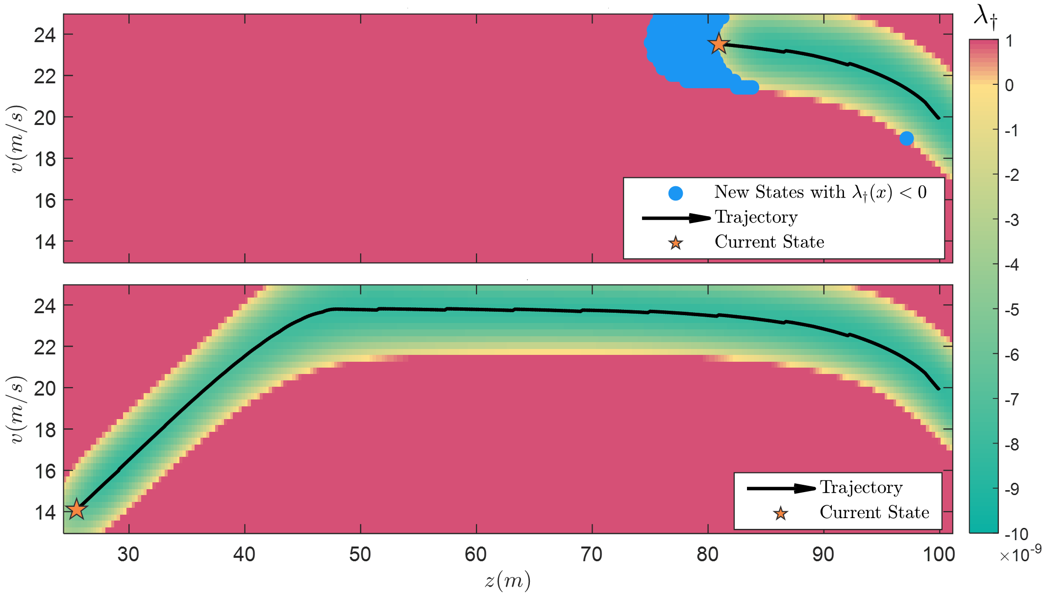
Figure 1: Color map of $\lambda_{\dagger}$ in the state-space of the adaptive cruise control system $x\!=\![v,z]^{T}$ when running Algorithm 1 with no prior data. The region in which $\lambda_{\dagger}<0$ is expanded online as Algorithm 1 collects new measurements. Top: snapshot when $\lambda_{\dagger}$ hits the threshold $-\varepsilon$, Algorithm 1 collects a measurement along $u_{\text{safe}}$ which expands the region where $\lambda_{\dagger}<0$ (in blue). Bottom: result at the end of the trajectory.

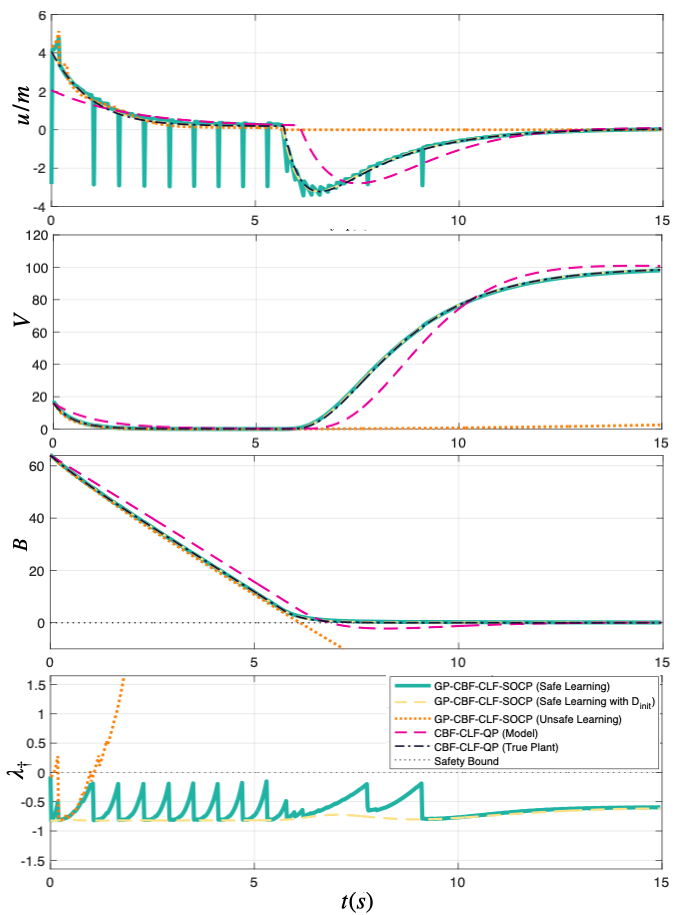
Figure 2: Simulation results of an adaptive cruise control system under model uncertainty, when controlled using different strategies: Algorithm 1 with no prior data (green); Algorithm 1 with a prior dataset (yellow); the GP-CBF-SOCP with no prior data using time-triggered updates online (orange); the CBF-QP using the uncertain dynamics (pink); and the oracle true-plant-based CBF-QP (black). Even when no prior data is available, Algorithm 1 keeps the system safe ($B>0$) by collecting measurements in the safety direction (negative $u$) when $\lambda_{\dagger}$ approaches $0$. This results in the ego car checking the brakes to reduce the uncertainty (negative spikes in the top plot). Using either the GP-CBF-SOCP with just time-triggered data collection, or the nominal model-based CBF-QP, the system becomes unsafe, as shown in the $B$ plot.

In this section, we test our framework on the following two examples in numerical simulation. The first example of an adaptive cruise control system highlights how the feasibility of the controller improves from the data collected online through Algorithm 1. The second example of a kinematic vehicle system demonstrates the applicability of our framework to multi-input systems.

7.1 Adaptive Cruise Control

We apply our proposed framework to a numerical model of an adaptive cruise control system

$$\dot{x}=f(x)+g(x)u,~{}~{}f(x)\!=\!\begin{bmatrix}-F_{r}(v)/m\\ v_{0}-v\end{bmatrix},\ g(x)\!=\!\begin{bmatrix}0\\ 1/m\end{bmatrix},$$ (33)

where $x\!=\![v,z]^{T}\in\mathbb{R}^{2}$ is the system state, with $v$ being the ego car’s velocity and $z$ the distance between the ego car and the car in front of it; $u\in\mathbb{R}$ is the ego car’s wheel force; $v_{0}$ is the constant velocity of the front car (14 m/s); $m$ is the mass of the ego car; and $F_{r}(v)\!=\!f_{0}\!+\!f_{1}v\!+\!f_{2}v^{2}$ is the rolling resistance force on the ego car. We introduce uncertainty in the mass and the rolling resistance.

A CLF is designed for stabilizing to a desired speed of $v_{d}=24$ m/s, and a CBF enforces a safe distance of $z\geq 1.8v$ with respect to the front vehicle. We specifically use $V(x)=(v-v_{d})^{2}$ and $B(x)\!=\!z\!-\!1.8v$. Following Remark 6, the CLF-based stability constraint is added as a soft constraint to the SOCP controller, replacing the reference control input $u_{\text{ref}}$. Therefore, the CBF acts as a hard safety constraint that filters a control policy based on the CLF whose objective is to stabilize the car to the desired speed $v_{d}$.

Figure 1 shows a state-space color map of the value of $\lambda_{\dagger}$ at two different stages of the trajectory generated running Algorithm 1 for the adaptive cruise control system with no prior data starting from $x_{0}=[20,100]^{T}$. The top plot represents an intermediate state, in which the system is still trying to reach the desired speed of $24$ m/s since the safety constraint (16b) is not active yet (the car in front is still far). Even though Algorithm 1 is collecting measurements in a time-triggered fashion using the SOCP (16) controller, the state gets close to the boundary of $\lambda_{\dagger}=0$ frequently, since the performance-driven control input obtained from the SOCP (16) when the safety constraint is not active is very different from $u_{\text{safe}}$. One such case is visualized in the top figure. However, Algorithm 1 detects that $\lambda_{\dagger}$ is getting close to zero and an event-triggered measurement in the direction of $u_{\text{safe}}$ is taken, which expands the region where $\lambda_{\dagger}<0$. The bottom plot shows the color map of $\lambda_{\dagger}$ at the end of the process, with the final dataset. The safety constraint was active for a portion of the trajectory (when the ego vehicle approached the front one and reduced its speed), and the system stayed safe by virtue of using Algorithm 1 to keep a direction $u_{\text{safe}}$ available.

Figure 2 shows that while a nominal CBF-QP (in pink) fails to keep the system safe under model uncertainty, Algorithm 1 with no prior data (in green) always manages to keep $B>0$ and $\lambda_{\dagger}<0$ by collecting measurements along $u_{\text{safe}}$ (negative spikes in the control input $u$ in the top plot) when triggered by the event $\lambda_{\dagger}\geq-\varepsilon$. The same algorithm without these event-triggered measurements fails (orange), since when the safety constraint (16b) becomes active, $\lambda_{\dagger}$ soon gets positive and the SOCP (16) becomes infeasible.

From another perspective, Figure 2 shows the importance of having a good nominal model or a prior database that properly characterizes a safe control direction. As shown in yellow, with such prior information Algorithm 1 keeps the system safe without having to take any measurements along $u_{\text{safe}}$. If no prior data is given, the control law is purely learned online, which leads to $\lambda_{\dagger}$ getting close to zero several times in the trajectory, and steps in the direction of $u_{\text{safe}}$ (negative $u$) are needed in order to prevent $\lambda_{\dagger}$ from actually reaching zero. This clearly damages the desired performance, as the car would be braking from time to time. Nevertheless, this is required in order to be certain about how the system reacts to pressing the brake. Therefore, the proposed event-triggered design allows Algorithm 1 to automatically reason about whether the available information is enough to preserve safety or the collection of a new data point along $u_{\text{safe}}$ is required instead. Note that our algorithm is also useful for cases in which a large dataset is available a priori, since it would secure safety even when the system is brought to out-of-distribution regions.

Figure 3: Illustration of the zero-level set of the CBF for the kinematic vehicle example. $D_{m}$ is the safety distance, which is computed by adding the minimum distance for the vehicle to steer with a maximal yaw rate without colliding with the obstacle $d_{steer}$ and a velocity-dependent distance margin $\tau(v-\underline{$v$})$.

7.2 Kinematic Vehicle

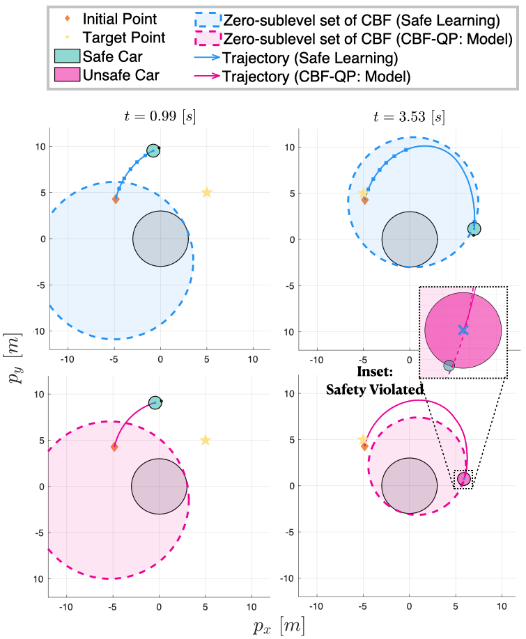
Figure 4: Snapshots that show the chronological evolution of a 4-dimensional kinematic vehicle system under model uncertainty, when controlled using different methods: Algorithm 1 with no prior data (top row, blue); the CBF-QP based on the nominal model (bottom row, pink). Starting at the initial state $x_{0}$ (orange diamond), the vehicle pursues the target (yellow star), while not colliding with the obstacle (grey circle). The curved line indicates the trajectory of the vehicle’s position that terminates with its position at the time when a snapshot is taken (green or red circle). Note that the circle is colored red when the vehicle violates the safety constraint (i.e., $B(x)<0$). The blue square positioned along the trajectory highlights the time stamps at which Algorithm 1 collects the data in event-triggered manner. Finally, the filled circle with a dotted border represents the zero-sublevel set of CBF. To watch the full video of the vehicle running under each control algorithm, please visit https://youtu.be/HM_VB_mGgeA.

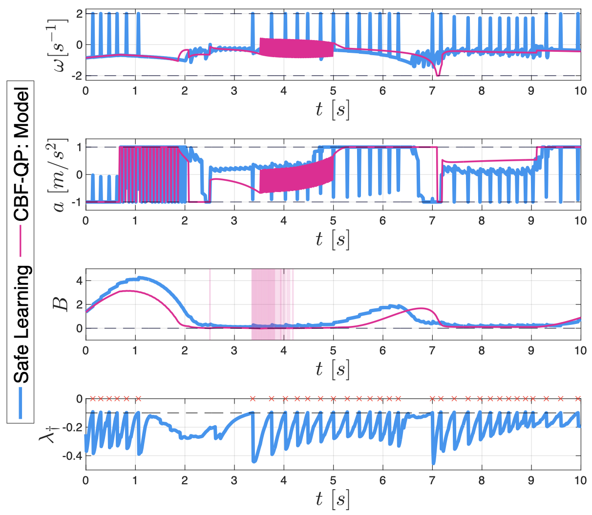
Figure 5: Simulation results of 4-dimensional kinematic vehicle system under model uncertainty, when using two strategies introduced in Figure 4 with the identical color notation. The four plots illustrate the yaw rate, the acceleration control inputs, the CBF values, and $\lambda_{\dagger}$ in time respectively. The dotted lines denote the input bounds, the zero-level of the CBF $B(x)=0$; and the threshold $-\epsilon$ in Algorithm 1. The red bars in the third plot represent the time stamps when the nominal CBF-QP violates safety. In contrast, Algorithm 1 ensures $B(x)>0$ at all times. The red cross points in the last plot indicate the time stamps when $\lambda_{\dagger}$ hits $-\epsilon$ and the safe exploration is executed according to Algorithm 1.

Next, in order to gauge our framework’s applicability to systems with higher state dimensions and multiple control inputs, we apply our method to a four-dimensional kinematic vehicle system. The state vector is denoted as $x\!=\![p_{x},p_{y},\theta,v]^{T}\in\mathbb{R}^{4}$ which consists of the vehicle’s position $(p_{x},p_{y})$, heading angle $\theta$, and longitudinal velocity $v$; the control input is denoted as $u\!=\![w,a]^{T}\in\mathbb{R}^{2}$ which includes the vehicle’s yaw rate $w\in[-\bar{w},\bar{w}]$ and the longitudinal acceleration $a\in[-\bar{a},\bar{a}]$. We use the values $\bar{a}=1$ and $\bar{w}=2$. The dynamics of the system are modeled as

$$\small f(x)\!=\!\begin{bmatrix}k_{v}v\cos\theta\\ k_{v}v\sin\theta\\ 0\\ -\mu v+s_{e}h(p_{x},p_{y})\end{bmatrix},\ g(x)\!=\!\begin{bmatrix}0&0\\ 0&0\\ k_{w}&0\\ 0&k_{a}\end{bmatrix},\normalsize$$ (34)

where $k_{v}$, $k_{w}$, $k_{a}$ are coefficients that capture the skid, the term $\mu v$ represents the drag, and $s_{e}h(p_{x},p_{y})$ accounts for the effect of the slope of the terrain. We assume that the nominal model does not address such effects (i.e., $k_{v}=k_{w}=k_{a}=1,\ \mu=s_{e}=0$), while the uncertainty imposed on the true system is induced by $k_{v}=2$, $k_{w}=1.5$, $k_{a}=1$, $\mu=0.5$, $s_{e}=0.5$, $h(p_{x},p_{y})=(p_{x}^{2}+p_{y}^{2})^{0.1}$. Note that unstructured uncertainties are imposed through terms like $h(p_{x},p_{y})$, which can be arbitrary functions, unlike the previous example that only imposes parametric uncertainties.

As illustrated in Figures 3 and 4, the objective of the control is to reach the target points alternating in time while not colliding into a static circular obstacle of radius $R_{o}=3$ centered at the origin. The reference controller $u_{\text{ref}}$ has two objectives: 1) it pursues a target point that alternates among a given set of points $S_{T}=\{(5,5),(5,-5),(-5,-5),(-5,5)\}$ every $p=2.5$ seconds, and 2) it stabilizes the vehicle’s velocity to $v_{d}$ while assuring that it is always bounded in $[\underline{$v$},\bar{v}]$. We use the values $\underline{$v$}=1$, $\bar{v}=5$, and $v_{d}=3$. All units are in the metric system.

The CBF we use is

$$B(x)\!=\!\sqrt{\left(p_{x}\!+\!\frac{D_{m}}{2}\cos\theta\right)^{2}\!+\!\left(p_{y}\!+\!\frac{D_{m}}{2}\sin\theta\right)^{2}}-\left(\!R_{o}\!+\!\frac{D_{m}}{2}\!\right),$$

where

$$D_{m}=\tau(v-\underline{v})+d_{steer};\quad d_{steer}=R_{o}\sqrt{1+\frac{2\bar{v}}{R_{o}\bar{w}}}-R_{o}.$$

This CBF adds a safety margin $D_{m}$ to the obstacle in the direction of the vehicle’s heading angle, based on its minimum velocity and maximum steering rate as shown in Figure 3. We can analytically check that the zero-superlevel set of the CBF is control invariant and that the CBF constraint is always feasible under the input bounds.

Figures 4 and 5 illustrate that while the CBF-QP based on the nominal model (in pink) escapes the zero-superlevel set of the CBF, Algorithm 1 (in blue) without any prior data always keeps the vehicle inside. This result not only demonstrates the validity of the proposed strategy when applied to a multi-input system but also alludes to the intuition behind our strategy: when $\lambda_{\dagger}$ hits $-\epsilon$, the vehicle steers away from the obstacle and decelerates more in order to improve the certainty of its safe control direction.

8 Conclusion

In this article, we have introduced a Control Barrier Function-based approach for the safe control of uncertain systems. Our results show that it is possible to guarantee the invariance of a safe set for an unknown system with high probability, by combining any available approximate model knowledge and sufficient data collected from the real system. We achieve this by first introducing a safety-critical optimization-based controller that, by formulation, is probabilistically robust to the prediction uncertainty of the unknown system’s dynamics. However, this optimization problem only produces a safe control action when the available information about the system (prior model knowledge and data) is sufficiently rich, as our feasibility analysis shows. As a means to fulfill this feasibility requirement, we later presented a formal method that, by collecting data online when required, is able to guarantee the recursive feasibility of the controller and therefore preserve the unknown system’s safety with high probability. Algorithm 1 presents a simple embodiment of this idea; however, we believe that future work should not be restricted to this particular implementation, since the most important contribution of this article is a principled reasoning procedure for conducting safe exploration when using data-driven control schemes.

Finally, we would like to emphasize that, as explained in Section 7, a practical takeaway from the results of this paper is that approximate model knowledge and prior data serve to reduce the conservatism of safety-assuring data-driven control approaches. We are convinced that designing control strategies with useful safety guarantees for uncertain systems requires combining model-based and data-driven methods, which until very recently were seen as mutually exclusive by experts in the field. With this research, we aim to present new evidence of the potential benefits of combining the two approaches.

[]Fernando Castañeda received a Ph.D. degree in mechanical engineering from the University of California, Berkeley in 2023. He is a Rafael del Pino Foundation Fellow (2020) and a “la Caixa” Foundation Fellow (2017). His research interests lie at the intersection of nonlinear control and data-driven methods, with a particular emphasis on ensuring the safe operation of high-dimensional systems in the real world.

[]Jason J. Choi (Student Member, IEEE) received the B.S. degree in mechanical engineering from Seoul National University in 2019. He is currently pursuing a Ph.D. degree at University of California Berkeley in mechanical engineering. His research interests center on optimal control theories for nonlinear and hybrid systems, data-driven methods for safe control, and their applications to robotics and autonomous mobility.

[]Wonsuhk Jung (Student Member, IEEE) received the B.S. degree in Mechanical Engineering and Artificial Intelligence from Seoul National University in 2022. He is currently pursuing a Ph.D. degree at Georgia Institute of Technology in Robotics. His research focuses on leveraging optimal control, planning, and data-driven methodologies for the safe operation of contact-rich robotics platforms.

[]Bike Zhang (Student Member, IEEE) received the B.Eng. degree in electrical engineering and automation from Huazhong University of Science and Technology in 2017. He is currently working toward the Ph.D. degree in mechanical engineering at University of California Berkeley. His current research interests include predictive control and reinforcement learning with application to legged robotics.

[] Claire J. Tomlin (Fellow, IEEE) is the James and Katherine Lau Professor of Engineering and professor and chair of the Department of Electrical Engineering and Computer Sciences (EECS) at UC Berkeley. She was an assistant, associate, and full professor in aeronautics and astronautics at Stanford University from 1998 to 2007, and in 2005, she joined UC Berkeley. She works in the area of control theory and hybrid systems, with applications to air traffic management, UAV systems, energy, robotics, and systems biology. She is a MacArthur Foundation Fellow (2006), an IEEE Fellow (2010), and in 2017, she was awarded the IEEE Transportation Technologies Award. In 2019, Claire was elected to the National Academy of Engineering and the American Academy of Arts and Sciences.

[] Koushil Sreenath (Member, IEEE) is an associate professor of mechanical engineering, at UC Berkeley. He received a Ph.D. degree in electrical engineering and computer science and a M.S. degree in applied mathematics from the University of Michigan at Ann Arbor, MI, in 2011. He was a postdoctoral scholar at the GRASP Lab at University of Pennsylvania from 2011 to 2013 and an assistant professor at Carnegie Mellon University from 2013 to 2017. His research interest lies at the intersection of highly dynamic robotics and applied nonlinear control. He received the NSF CAREER, Hellman Fellow, Best Paper Award at the Robotics: Science and Systems (RSS), and the Google Faculty Research Award in Robotics.

References

- [1] A. D. Ames, X. Xu, J. W. Grizzle, and P. Tabuada, “Control barrier function based quadratic programs for safety critical systems,” IEEE Transactions on Automatic Control, vol. 62, pp. 3861–3876, 2017.
- [2] S. Bansal, M. Chen, S. Herbert, and C. J. Tomlin, “Hamilton-jacobi reachability: A brief overview and recent advances,” in 2017 56th IEEE Conference on Decision and Control (CDC), 2017.
- [3] K. P. Wabersich and M. N. Zeilinger, “A predictive safety filter for learning-based control of constrained nonlinear dynamical systems,” Automatica, vol. 129, p. 109597, 2021.
- [4] Q. Nguyen and K. Sreenath, “L1 adaptive control for bipedal robots with control lyapunov function based quadratic programs,” in American Control Conference, Chicago, IL, July 2015, pp. 862–867.
- [5] A. J. Taylor and A. D. Ames, “Adaptive safety with control barrier functions,” in American Control Conference, 2020, pp. 1399–1405.
- [6] B. T. Lopez, J.-J. E. Slotine, and J. P. How, “Robust adaptive control barrier functions: An adaptive and data-driven approach to safety,” IEEE Control Systems Letters, vol. 5, no. 3, pp. 1031–1036, 2020.
- [7] M. Black and D. Panagou, “Adaptation for validation of a consolidated control barrier function based control synthesis,” arXiv preprint arXiv:2209.08170, 2022.
- [8] Q. Nguyen and K. Sreenath, “Robust safety-critical control for dynamic robotics,” IEEE Transactions on Automatic Control, 2021.
- [9] J. J. Choi, D. Lee, K. Sreenath, C. J. Tomlin, and S. L. Herbert, “Robust control barrier–value functions for safety-critical control,” in 2021 60th IEEE Conference on Decision and Control (CDC). IEEE, 2021, pp. 6814–6821.
- [10] S. Kolathaya and A. D. Ames, “Input-to-state safety with control barrier functions,” IEEE control systems letters, vol. 3, no. 1, pp. 108–113, 2018.
- [11] A. Alan, A. J. Taylor, C. R. He, A. D. Ames, and G. Orosz, “Control barrier functions and input-to-state safety with application to automated vehicles,” IEEE Transactions on Control Systems Technology, 2023.
- [12] M. Krstic, “Inverse optimal safety filters,” arXiv preprint arXiv:2112.08225, 2021.
- [13] A. J. Taylor, V. D. Dorobantu, H. M. Le, Y. Yue, and A. D. Ames, “Episodic learning with control lyapunov functions for uncertain robotic systems,” in IEEE/RSJ International Conference on Intelligent Robots and Systems, 2019, pp. 6878–6884.
- [14] A. J. Taylor, A. Singletary, Y. Yue, and A. Ames, “Learning for safety-critical control with control barrier functions,” in Learning for Dynamics and Control, 2020, pp. 708–717.
- [15] T. Westenbroek, F. Castañeda, A. Agrawal, S. S. Sastry, and K. Sreenath, “Learning min-norm stabilizing control laws for systems with unknown dynamics,” in IEEE Conference on Decision and Control, 2020, pp. 737–744.
- [16] J. Choi, F. Castañeda, C. Tomlin, and K. Sreenath, “Reinforcement Learning for Safety-Critical Control under Model Uncertainty, using Control Lyapunov Functions and Control Barrier Functions,” in Robotics: Science and Systems, Corvalis, OR, 2020.
- [17] F. Berkenkamp, R. Moriconi, A. P. Schoellig, and A. Krause, “Safe learning of regions of attraction for uncertain, nonlinear systems with gaussian processes,” in IEEE Conference on Decision and Control, 2016, pp. 4661–4666.
- [18] F. Berkenkamp, M. Turchetta, A. Schoellig, and A. Krause, “Safe model-based reinforcement learning with stability guarantees,” in Advances in Neural Information Processing Systems. Curran Associates, Inc., 2017, vol. 30, pp. 908–918.
- [19] J. F. Fisac, A. K. Akametalu, M. N. Zeilinger, S. Kaynama, J. Gillula, and C. J. Tomlin, “A general safety framework for learning-based control in uncertain robotic systems,” IEEE Transactions on Automatic Control, vol. 64, no. 7, pp. 2737–2752, 2018.
- [20] J. Umlauft, L. Pöhler, and S. Hirche, “An uncertainty-based control lyapunov approach for control-affine systems modeled by gaussian process,” IEEE Control Systems Letters, vol. 2, pp. 483–488, 2018.
- [21] D. D. Fan, J. Nguyen, R. Thakker, N. Alatur, A. a. Agha-mohammadi, and E. A. Theodorou, “Bayesian learning-based adaptive control for safety critical systems,” in IEEE International Conference on Robotics and Automation, 2020, pp. 4093–4099.
- [22] R. Cheng, M. J. Khojasteh, A. D. Ames, and J. W. Burdick, “Safe multi-agent interaction through robust control barrier functions with learned uncertainties,” in IEEE Conference on Decision and Control, 2020, pp. 777–783.
- [23] M. H. Cohen and C. Belta, “Safe exploration in model-based reinforcement learning using control barrier functions,” arXiv preprint arXiv:2104.08171, 2021.
- [24] F. Castañeda, J. J. Choi, B. Zhang, C. J. Tomlin, and K. Sreenath, “Gaussian process-based min-norm stabilizing controller for control-affine systems with uncertain input effects and dynamics,” in American Control Conference, 2021.
- [25] F. Castañeda, J. J. Choi, B. Zhang, C. J. Tomlin, and K. Sreenath, “Pointwise feasibility of gaussian process-based safety-critical control under model uncertainty,” in IEEE Conference on Decision and Control, 2021, pp. 6762–6769.
- [26] A. J. Taylor, V. D. Dorobantu, S. Dean, B. Recht, Y. Yue, and A. D. Ames, “Towards robust data-driven control synthesis for nonlinear systems with actuation uncertainty,” in IEEE Conference on Decision and Control, 2021, pp. 6469–6476.
- [27] M. Greeff, A. W. Hall, and A. P. Schoellig, “Learning a stability filter for uncertain differentially flat systems using gaussian processes,” in IEEE Conference on Decision and Control, 2021, pp. 789–794.
- [28] V. Dhiman, M. J. Khojasteh, M. Franceschetti, and N. Atanasov, “Control barriers in bayesian learning of system dynamics,” IEEE Transactions on Automatic Control, 2021.
- [29] L. Brunke, S. Zhou, and A. P. Schoellig, “Barrier bayesian linear regression: Online learning of control barrier conditions for safety-critical control of uncertain systems,” in Learning for Dynamics and Control, 2022, pp. 881–892.
- [30] J. Umlauft and S. Hirche, “Feedback linearization based on gaussian processes with event-triggered online learning,” IEEE Transactions on Automatic Control, vol. 65, no. 10, pp. 4154–4169, 2019.
- [31] H. K. Khalil and J. W. Grizzle, Nonlinear systems. Prentice Hall, Upper Saddle River, NJ, 2002, vol. 3.
- [32] X. Xu, P. Tabuada, J. W. Grizzle, and A. D. Ames, “Robustness of control barrier functions for safety critical control,” IFAC-PapersOnLine, vol. 48, no. 27, pp. 54–61, 2015.
- [33] C. Dawson, Z. Qin, S. Gao, and C. Fan, “Safe nonlinear control using robust neural lyapunov-barrier functions,” in Conference on Robot Learning. PMLR, 2022, pp. 1724–1735.
- [34] Z. Qin, D. Sun, and C. Fan, “Sablas: Learning safe control for black-box dynamical systems,” IEEE Robotics and Automation Letters, vol. 7, no. 2, pp. 1928–1935, 2022.
- [35] P. Jagtap, G. J. Pappas, and M. Zamani, “Control barrier functions for unknown nonlinear systems using gaussian processes,” in 2020 59th IEEE Conference on Decision and Control (CDC). IEEE, 2020, pp. 3699–3704.
- [36] L. Lindemann, A. Robey, L. Jiang, S. Tu, and N. Matni, “Learning robust output control barrier functions from safe expert demonstrations,” arXiv preprint arXiv:2111.09971, 2021.
- [37] W. Jin, Z. Wang, Z. Yang, and S. Mou, “Neural certificates for safe control policies,” arXiv preprint arXiv:2006.08465, 2020.
- [38] D. Duvenaud, “Automatic model construction with gaussian processes,” Ph.D. dissertation, University of Cambridge, 2014.
- [39] N. Srinivas, A. Krause, S. Kakade, and M. Seeger, “Gaussian process optimization in the bandit setting: No regret and experimental design,” in International Conference on Machine Learning, 2010.
- [40] H. Wendland, Scattered data approximation. Cambridge university press, 2004, vol. 17.
- [41] J. Umlauft, T. Beckers, A. Capone, A. Lederer, and S. Hirche, “Smart forgetting for safe online learning with gaussian processes,” in Learning for Dynamics and Control, 2020, pp. 160–169.
- [42] H. Liu, Y.-S. Ong, X. Shen, and J. Cai, “When gaussian process meets big data: A review of scalable gps,” IEEE transactions on neural networks and learning systems, vol. 31, no. 11, pp. 4405–4423, 2020.
- [43] S. Dean, A. Taylor, R. Cosner, B. Recht, and A. Ames, “Guaranteeing safety of learned perception modules via measurement-robust control barrier functions,” in Conference on Robot Learning, 2021.
- [44] J. Buch, S.-C. Liao, and P. Seiler, “Robust control barrier functions with sector-bounded uncertainties,” IEEE Control Systems Letters, vol. 6, pp. 1994–1999, 2021.
- [45] T. Lew, A. Sharma, J. Harrison, E. Schmerling, and M. Pavone, “On the problem of reformulating systems with uncertain dynamics as a stochastic differential equation,” arXiv preprint arXiv:2111.06084, 2021.
- [46] F. Zhang, The Schur complement and its applications. Springer Science & Business Media, 2006, vol. 4.
- [47] G. Still, “Lectures on parametric optimization: An introduction,” Optimization Online, 2018.
- [48] N. Andréasson, A. Evgrafov, and M. Patriksson, An introduction to continuous optimization: foundations and fundamental algorithms. Courier Dover Publications, 2020.
- [49] J. Lygeros, K. H. Johansson, S. N. Simic, J. Zhang, and S. S. Sastry, “Dynamical properties of hybrid automata,” IEEE Transactions on Automatic Control, vol. 48, no. 1, pp. 2–17, 2003.
[![[Uncaptioned image]](/html/2208.10733/assets/authors/fernando.jpg) ]Fernando Castañeda received a Ph.D. degree in mechanical engineering from the University of California, Berkeley in 2023. He is a Rafael del Pino Foundation Fellow (2020) and a “la Caixa” Foundation Fellow (2017). His research interests lie at the intersection of nonlinear control and data-driven methods, with a particular emphasis on ensuring the safe operation of high-dimensional systems in the real world.