Invariants of Weakly successively almost positive links

Abstract.

As an extension of positive and almost positive diagrams and links, we study two classes of links we call successively almost positive and weakly successively almost positive links.

We prove various properties of polynomial invariants and signatures of such links, extending previous results or answering open questions about positive or almost positive links. We discuss their minimal genus and fibering property and for the latter prove a fibering extension of Scharlemann-Thompson’s theorem (valid for general links).

1. Introduction

1.1. Background and motivation

A link diagram is positive if all the crossings are positive, and a positive link is a link that can be represented by a positive diagram. Positive links have various nice properties and form an important class of links.

A suggestive generalization of a positive diagram is a $k$-almost positive diagram, a diagram such that all but $k$ crossings are positive. A $1$-almost positive diagram is usually called an almost positive diagram and has been studied in various places.

It is known that almost positive links share various properties with positive links. However, although there are some special properties of $2$- or $3$-almost positive links as discussed in [PT], when $k$ is large, $k$-almost positive links fail to have nice properties similar to positive links because every knot $K$ is $k$-almost positive for sufficiently large $k$. Indeed, as we will frequently see (Example 6.8) even for $2$-almost positive knots, almost all properties of positive links fail.

The aim of this paper is to propose and investigate natural generalizations of a(n almost) positive diagram.

We introduce various classes of diagrams which are generalizations of (almost) positive diagrams (see Section 1.2 for a concise summary of the definitions of these generalizations). Unlike almost positive diagrams, the class we introduce can have arbitrary many negative crossings. Nevertheless, these diagrams share various properties with (almost) positive links.

Among them, weakly successively almost positive links, the central object which we study in this paper, provide a unified and satisfactory framework to treat the positivity of diagrams. One crucial feature of this class of diagrams is that it is closed under the skein resolution in a suitable way (Theorem 5.4) that allows to use an induction argument.

We will prove various properties of (weakly) successively almost positive links which extend known results of (almost) positive links. Frequently our results are new even for the positive links, or answer questions about (almost) positive links that appeared in the literature. (For instance, see Corollary 6.5 or Corollary 8.3.) Thus weakly successively almost positive diagrams/links provide a better framework to study positive diagrams.

1.2. Summaries of various positivities

To begin with, for the reader’s convenience, we list the definitions of various positivities discussed or studied in the paper.

Definition 1.1.

Let $D$ be a link diagram $D$ and $k\in\mathbb{Z}_{\geq 0}$ be a non-negative integer.

• $D$ is positive if all the crossings of $D$ are positive.

• $D$ is almost positive if all but $1$ crossing of $D$ are positive. Almost positive diagrams are divided into the following two types.

  • We say that $D$ is of type I if the negative crossing $c$ of $D$ connects two Seifert circles $s$ and $s^{\prime}$, so that there is no other (positive) crossing connecting $s$ and $s^{\prime}$.

  • Otherwise, we say that $D$ is of type II.

• $D$ is successively $k$-almost positive if all but $k$ crossings of $D$ are positive, and the $k$ negative crossings appear successively along a single overarc (see Definition 3.1).

• $D$ is good successively $k$-almost positive if $D$ is successively $k$-almost positive and for a negative crossing $c$ of $D$ that connects two Seifert circles $s$ and $s^{\prime}$, there are no other crossing connecting $s$ and $s^{\prime}$ (see Definition 3.3).

• $D$ is weakly successively $k$-almost positive if all but $k$ crossings of $D$ are positive, and the $k$ negative crossings appear (but not necessarily consecutively) along a single overarc which we call negative overarc (see Definition 5.1 and Figure 6).

• $D$ is weakly positive if $D$ can be viewed as a descending diagram except at positive crossings; when we walk along $D$, we pass every negative crossing first (see Definition 4.1), through its overpass.

In the following we use abbreviations in the paper to save space.

• s.a.p.: successively almost positive.

• $k$-s.a.p.: successively $k$-almost positive.

• w.s.a.p.: weakly successively almost positive.

• $k$-w.s.a.p.: weakly successively $k$-almost positive.

A link $L$ is positive if $L$ is represented by a positive diagram. An almost positive link, successively almost positive link,… is defined by the same manner.

There are other types of positivities of links which are defined by braid representatives, not diagrams.

Definition 1.2.

A link $L$ is

• braid positive (or, a positive braid link) if $L$ is represented by a closure of a a positive braid.

• strongly quasipositive if $L$ is represented by a closure of a strongly quasipositive braid, a product of braids $\{(\sigma_{i}\sigma_{i+1}\cdots\sigma_{j-2})\sigma_{j-1}(\sigma_{i}\sigma_{i+1}\cdots\sigma_{j-2})^{-1}\>|\>1\leq i<j\leq n\}$ (see Definition 2.16).

• quasipositive if $L$ is represented by a closure of a quasiposisitve braid, a product of braids of the form $\{\alpha\sigma_{1}\alpha^{-1}\>|\>\alpha\in B_{n}\}$.

In our investigations, the following property also plays a fundamental role (see Section 2.9 for details and background).

Definition 1.3.

A link $L$ is Bennequin-sharp if the Bennequin inequality is an equality.

The positive and almost positive links have appeared and have been studied in past publications and enjoyed extensive treatment (for example, [Cr, St3]).

The successively almost positive links, and the good successively almost positive links were introduced and studied in [It3]. The current work grew out of the investigation of natural problems raised in [It3].

The weakly successively almost positive links are the main objects which we introduce and study in the paper. This notion has occurred (without extra prominence lent) in Cromwell’s construction of positive skein trees ([Cr, Theorem 2]), and is a natural generalization of successively almost positive links.

The weakly positive diagrams/links is the largest class of links that enjoys certain positivity phenomena.

Positive braid links are the natural positive object in the braid group point of view. Strongly quasipositive links and quasipositive links have their origins in Rulodph’s works [Rud1],[Rud3] and although it is not clear from the above definition, they are more related to the positivity of Seifert surfaces. Recently these positivity notions gather much attention due to close connection to the contact topology, like the Bennequin-sharp property.

The relations among these positivities are summarized in the following diagram.

Figure 1. Summary of relations of various positivity notions

For the less obvious inclusions, compare the explanation below Definition 3.3.

We will show in Section 11 that all of the inclusions in the above chart which are indicated so are strict, so that (weakly) successively almost positive links form a strictly new class of links. (See also Question 12.1, and Question 12.2, but also Remark 11.2.)

1.3. Organization of the paper and summary of results

In Section 2 we set up notation and terminology, and review various standard facts in knot theory which will be used in the paper.

Section 3 provides a quick review of a successively positive link, the content of [It3]. The content of Section 3 gives a motivation and prototype of various results proven in the paper.

In Section 4 we introduce a weakly positive diagram. It is crucial that a weakly positive diagram ‘obviously’ tells us whether it represents a split link or not (Theorem 4.5). This special feature leads to several properties of the Conway polynomial, which will be frequently used in the rest of the paper,

Our main object, a weakly successively almost positive diagram, is introduced in Section 5. From its definition, it is clear that it admits a standard skein triple, a skein triple that consists of weakly successively almost positive diagrams reducing its complexity (Theorem 5.4). Using the fact that a weakly successively almost positive diagram is weakly positive, we can pin down when a split link appears in the standard skein triple (Lemma 5.5). Also, we have a standard unknotting/unlinking sequence, a sequence of crossing changes that converts a w.s.a.p. link into the unlink. These sequences play a fundamental role in our study of weakly successively almost positive links.

Section 6 establishes various illuminating properties of the Conway polynomial of weakly successively almost positive links (Theorem 6.4, Proposition 6.10). They are far-reaching generalizations of properties of the Conway polynomials of positive links and contain a new result even for positive links.

Section 7 is devoted to the HOMFLY polynomial of weakly successively almost positive links (Theorem 7.1). We will also discuss the properties of Jones polynomials (Theorem 7.4). As we will frequently mention in various examples, the property of the HOMFLY polynomial (Theorem 7.1) is quite strong to show that a given knot is not weakly successively almost positive.

Section 8 provides an enhancement of results in the previous two sections (Theorem 8.1), under the additional assumption that $L$ is Bennequin-sharp. We demonstrate, under this additional assumption, the Conway and HOMFLY polynomial of weakly successively almost positive links have more special properties.

They motivate the question how to exhibit w.s.a.p. links as Bennequin-sharp. This is a separate long topic that has to be moved out to a follow-up paper [IS]. There we will give extensive treatment of Seifert surfaces and also explain the relation to strong quasipositivity.

Section 9 is devoted to the positivity of the signature; we prove that a non-trivial weakly successively almost positive link has strictly positive signature (Theorem 9.1), generalizing the (almost) positive link case. We discuss various applications of the positivity of the signature. Among them, we present several delicate examples of knots which are not weakly successively almost positive, but its knot polynomials share the same properties as we have proved in Section 6, Section 7.

Section 10 establishes a more general signature inequality. We prove a signature estimate from a general link diagram (Theorem 10.1), which improves the signature estimate given by Baader-Dehornoy-Liechti [BDL]. As an application, we prove that every algebraic knot concordance class contains only finitely many weakly successively $k$-almost positive links (Theorem 10.3).

Section 11 establishes the strictness of inclusions for various classes of positivities (Theorem 11.1). Since our results says that weakly successively almost positive links and (almost) positive links share many properties, it is not surprising that showing a given weakly successively almost positive link is not (almost) positive is subtle.

Section 12 gathers various questions for (weakly) successively almost positive links.

The paper contains two appendices. In Appendix A we prove Theorem 6.2, a slight enhancement of Scharlemann-Thompson’s theorem of Euler characteristics of skein triples that tells us the fiberedness property, which was used in the proof of Theorem 6.4. We review some background on sutured manifold theory and the proof of Scharlemann-Thompson’s theorem (Theorem 6.1), then we explain how to get the fibration information.

In Appendix B we determine which knots are (weakly) successively almost positive, for all prime knots to 12 crossings, with four exceptions.

2. Preparation

In this section we prepare various notions which will be used in the paper. We summarize our notation, conventions and terminologies.

In the following, we usually assume that a link diagram $D$ is always oriented. We will usually regard a diagram $D$ is contained in $\mathbb{R}^{2}$, not $S^{2}$, although we will sometimes utilize an isotopy of diagram in $S^{2}$ to make the situation simple.

We denote by $c(D)$ the number of crossings of $D$, and we denote by $c_{+}(D)$ (resp. $c_{-}(D)$) the number of positive (resp. negative) crossings. We write $w(D)=c_{+}(D)-c_{-}(D)$ for the writhe of $D$.

An inequality $a\geq b$ is exact if $a=b$, and strict otherwise.

2.1. Primeness and splitness

For a link $L$, we denote by $\#L$ the number of its components.

We use $L_{1}\#L_{2}$, as a binary operation, for the connected sum of the links $L_{1}$ and $L_{2}$ (although when $\#L\geq 2$, it is not uniquely determined). We write $\#^{n}L$ for the ($n-1$-fold iterated) connected sum of $n$ copies of a link $L$. Thus $\#^{1}L=L$ (which is not to be confused with the integer $\#L$). By convention, we always regard $\#^{0}L$ as the unknot, regardless the number of components.

We say that a link $L$ is prime if, whenever $L=K_{1}\#K_{2}$, then (exactly) one of $K_{1}$ and $K_{2}$ is an unknot. Another way of saying this is that a link is prime if every $S^{2}\subset S^{3}$ which intersects the link in two points (transversely), leaves an unknotted arc on (exactly) one side of the $S^{2}$.

We say a link is split if there is some $S^{2}\subset S^{3}$ which intersects the link nowhere, but leaves parts of the link on either side of the $S^{2}$. We call such $S^{2}$ a splitting sphere.

We say two components $K_{1},K_{2}$ of a link $L$ are inseparable, if there is no splitting sphere of $L$ containing $K_{1}$, $K_{2}$ on opposite sides. The equivalence classes of components of $L$ with respect to the inseparability relation are the split components of $L$. We write

$$L=L_{1}\sqcup L_{2}\sqcup\cdots\sqcup L_{m}$$

as the split union of its split components $L_{i}$.

Such split components may of course in general contain several components of $L$. We say that $L$ is a totally split link, if each split component of $L$ contains exactly one component of $L$.

The totally split link whose $n$ (split) components are unknots is the ($n$-component) unlink, and will be denoted $U_{n}$. For simplicity we write $U_{1}=\bigcirc$ for the unknot.

2.2. Seifert’s algorithm and Seifert graph

In this section we review Seifert’s algorithm and related notions.

For an oriented link diagram $D$ and a crossing $c$ of $D$, the smoothing at $c$ is a diagram $D$ obtained by replacing the crossing $c$ as

$$\raisebox{-7.11317pt}{ \begin{picture}(24.0,24.0)\put(10.0,14.0){\vector(-1,1){10.0}} \put(24.0,0.0){\line(-1,1){10.0}} \put(0.0,0.0){\vector(1,1){24.0}} \end{picture} }\longrightarrow\raisebox{-7.11317pt}{ \begin{picture}(24.0,24.0)\qbezier(0.0,0.0)(14.0,12.0)(0.0,24.0)\qbezier(24.0,0.0)(10.0,12.0)(24.0,24.0)\put(24.0,24.0){\vector(1,1){0.0}} \put(0.0,24.0){\vector(-1,1){0.0}} \end{picture} }\longleftarrow\raisebox{-7.11317pt}{ \begin{picture}(24.0,24.0)\put(0.0,0.0){\line(1,1){10.0}} \put(14.0,14.0){\vector(1,1){10.0}} \put(24.0,0.0){\vector(-1,1){24.0}} \end{picture} }$$

according to its sign.

A triple of diagrams $(D_{+},D_{0},D_{-})$ equal except as designated above, or the triple of their corresponding links $(L_{+},L_{0},L_{-})$, is called a skein triple.

By smoothing all the crossings of $D$, we get a disjoint union of circles. A Seifert circle of $D$ is its connected component. We denote the number of Seifert circles by $s(D)$.

Each Seifert circle $s$ separates the projection plane $\mathbb{R}^{2}$ into two components of $\mathbb{R}^{2}\setminus s$. One is compact, which we call interior of $s$ , and the other is non-compact, which we call its exterior. For Seifert circles $s$ and $s^{\prime}$, we say that $s$ is contained in $s^{\prime}$ if $s$ belongs to the interior of $s$.

A Seifert circle $s$ is separating if both its interior and exterior contain other Seifert circles.

For each Seifert circle $s$, we take a disk $d_{s}$ in $\mathbb{R}^{3}$ bounded by Seifert circles having constant $z$-coordinate (height) $h_{s}$. We choose $h_{s}$ so that they are pairwise distinct and that

$$h_{s}>h_{s^{\prime}}\mbox{ whenever }s\mbox{ is contained in }s^{\prime}.$$ (2.1)

Then we connect these disks by attaching twisted bands at the crossing to get Seifert surface $S_{D}$ of $L$.

Definition 2.1 (Canonical Seifert surface, canonical genus).

The Seifert surface $S_{D}$ is called the canonical Seifert surface of $D$. The canonical Euler characteristic $\chi(D)$ of $D$ is defined by

$$\chi(D)=\chi(S_{D})=s(D)-c(D).$$

The canonical genus of a diagram $D$ is defined by

$$g(D)=\frac{-\chi(D)-\#L+2}{2}$$

In the following, we will often identify the crossing $c$ with a twisted band in the canonical Seifert surface. For example, we say that a crossing $c$ connects Seifert circles $s$ and $s^{\prime}$ if the twisted band of $S_{D}$ that corresponds to $c$ connects the disks bounded by $s$ and $s^{\prime}$.

To encode the structure of a diagram and its canonical Seifert surface, we will use the following graph.

Definition 2.2.

The Seifert graph $\Gamma(D)$ of a diagram $D$ is bipartite graph without self-loop, whose set of vertices of $\Gamma(D)$ is the set of Seifert circles, and whose set of edges is the set of crossings. A crossing $c$ connecting Seifert circles $s$ and $s^{\prime}$ corresponds to an edge of $\Gamma(D)$ connecting the corresponding vertices. We often view $\Gamma(D)$ as a signed graph. Each edge carries a sign $\pm$ according to the sign of the crossing.

To analyse the properties of (Seifert) graphs, we will use the following terminology.

• An edge $e$ is singular if there is no other edge connecting the same vertices as $e$.

• An edge $e$ is called an isthmus if removing the edge $e$ makes the graph disconnected.

• Let $v_{1}$ (resp. $v_{2}$) be a vertex of a graph $\Gamma_{1}$ (resp. $\Gamma_{2}$), The one-point join $\Gamma_{1}\ast_{v_{1}=v_{2}}\Gamma_{2}$ is a graph obtained by identifying $v_{1}$ and $v_{2}$.

  Although the choice of $v_{1},v_{2}$ is obviously necessary, we often write $\Gamma_{1}*\Gamma_{2}$ for the result of this operation under some choice of $v_{1}$ and $v_{2}$. (In this loose sense, $*$ becomes both a commutative and associative operation.)

2.3. Diagrams and crossings

In this section we recall terminology related to diagrams and crossings.

A region of a link diagram $D$ is a connected component of the complement of $\mathbb{R}^{2}\setminus D$ (or, $S^{2}\setminus D$). Every crossing $c$ of $D$ is adjacent to four regions. To illustrate their relations we use the following terms.

Definition 2.3.

We say that a region $R$ around the crossing $c$ is a Seifert circle region near $c$ if, near the crossing $c$ the regions contains pieces of Seifert circles near $c$. We say that regions $R$ and $R^{\prime}$ around the crossing $c$ are

• opposite (at $c$) if they do not share an edge.

• neighbored (at $c$) if they share an edge near $c$.

Similarly, to describe how the crossing connects two Seifert circles, we use the following notions.

Definition 2.4.

Let $c,c^{\prime}$ be crossings of a diagram $D$.

• $c$ and $c^{\prime}$ are Seifert equivalent if they connect the same pair of (distinct) Seifert circles.

• $c$ and $c^{\prime}$ are twist equivalent if one of their pairs of opposite regions coincides.

• $c$ and $c^{\prime}$ are $\sim$-equivalent if their pairs of opposite non-Seifert circle regions coincide.

• $c$ and $c^{\prime}$ are $\stackrel{{\scriptstyle\displaystyle\sim}}{{\vbox{\vskip-1.99997pt\hbox{$\scriptstyle*$}}}}$-equivalent if their the pairs of opposite Seifert circle regions coincide.

By definition, $\stackrel{{\scriptstyle\displaystyle\sim}}{{\vbox{\vskip-1.99997pt\hbox{$\scriptstyle*$}}}}$-equivalent implies Seifert equivalent. The converse is not true in general, because Seifert circles do not border unique regions. However, if the diagram is special (see below definition), the converse is true.

Finally we summarize various notions of diagrams which we be used or discussed.

Definition 2.5.

We say that a link diagram $D$ is

• reduced if it contains no nugatory (reducib;e) crossings. Here a crossing $c$ of $D$ is nugatory (reducible) if there exists a circle $c$ in $\mathbb{R}^{2}$ that transversely intersects with $D$ only at $c$.

• special if it contains no separating Seifert circles.

• split if it is disconnected, as a subspace in $\mathbb{R}^{2}$.

• non-prime (composite) if there is a simple closed curve $c$ that transversely intersects with $c$, so that for the connected components $U,V$ of $\mathbb{R}^{2}\setminus c$, both $U\cap D$ and $V\cap D$ are not embedded arcs. Otherwise, we say that $D$ is prime.

2.4. Genera of links

The genus and the slice genus (smooth 4-ball genus) of a link $L$ is defined by

$$g(L)=\frac{-\chi(L)-\#L+2}{2},\quad g_{4}(L)=\frac{-\chi_{4}(L)-\#L+2}{2}$$ (2.2)

respectively. Here $\chi(L)$ is the maximum Euler characteristic of Seifert surface of $L$, and $\chi_{4}(L)$ is the maximum Euler characteristic of 4-ball surface, a smoothly embedded surface in $B^{4}$ whose boundary is $L$.

Remark 2.6.

The definition of genus assumes that a maximal Euler characteristic Seifert surface or 4-ball surface is connected. As we will see later, this implicit assumption is satisfied whenever $L$ is a non-split weakly positive link, because of linking number reasons (see Corollary 4.9).

But regardless of the connectivity issue, for now we use $g_{4}$ and $g$ just as quantities defined as above. Certainly when $L$ is a knot, a surface is connected, so that the (4-ball) genus is correctly reflected.

As a quantity related to diagrams, we use the following.

Definition 2.7.

The canonical genus of a link $L$ is defined by

$$g_{c}(L)=\min\{g(D)\>|\>D\mbox{ is a diagram of }L\}$$

By convention, for a diagram $D$ of $L$ we put $g_{4}(D)=g_{4}(L)$ and $\chi_{4}(D)=\chi_{4}(L)$.

Obviously for every link $L$, the inequality

$$g_{4}(L)\leq g(L)\leq g_{c}(L)\,.$$

holds.

2.5. Murasugi sum and diagram Murasugi sum

The Murasugi sum is an operation on surfaces that generalizes the connected sum, and has very nice features, as indicated in the title ‘the Murasugi sum is a natural geometric operation’ of the papers by Gabai [Ga, Ga3].

Definition 2.8 (Murasugi sum (of surfaces in $S^{3}$)).

Let $R_{1}$ and $R_{2}$ be oriented surfaces with boundary. An oriented surface $R$ in $S^{3}$ is a Murasugi sum of $R_{1}$ and $R_{2}$ if there is a 2-sphere $S\subset S^{3}$ that separates $S^{3}$ into two 3-balls $B_{1}$ and $B_{2}$, such that

1. $R_{1}\subset B_{1}$, $R_{2}\subset B_{2}$.

2. $D:=R_{1}\cap S=R_{2}\cap S$ is a $2n$-gon.

We often say that $R$ is a Murasugi sum of $R_{1}$ and $R_{2}$ along the $2n$-gon $D$.

We use the following diagram version of Murasugi sum which is often called the $\ast$-product.

Definition 2.9 (Diagram Murasugi sum).

Let $D_{1}$ be a (planar, in $\mathbb{R}^{2}$) link diagram and $s_{1}$ be an innermost Seifert circle of $D_{1}$; this means $s_{1}$ bounds a disk whose interior contains no other Seifert circles of $D_{1}$. Similarly, let $D_{2}$ be a link diagram and $s_{2}$ be an outermost Seifert circle of $D_{2}$ (i.e., whose exterior does not contain any other Seifert circle).

The diagram Murasugi sum (or, $\ast$-product) $D_{1}\ast D_{2}$ is a link diagram obtained by identifying $s_{1}$ and $s_{2}$. See Figure 2. We often write $D_{1}\ast_{s_{1}=s_{2}}D_{2}$ to indicate the identified Seifert circles. The resulting Seifert circle is separating.

The diagram Murasugi sum is not uniquely determined by $(D_{1},s_{1})$ and $(D_{2},s_{2})$ since there is a freedom to choose how the crossings connected to $s_{1}$ and $s_{2}$ align along the identified Seifert circle $s_{1}=s_{2}$. For the canonical Seifert surface $S_{D_{1}\ast D_{2}}$ of $D_{1}\ast D_{2}$ is the Murasugi sum of the canonical Seifert surfaces $S_{D_{1}}$ and $S_{D_{2}}$ along the disks bounded by $s_{1}$ and $s_{2}$.

Figure 2. Diagram Murasugi sum of $D_{1}$ and $D_{2}$ along their Seifert circles $s_{1}$, $s_{2}$.

On the other hand, on the level of Seifert graphs, the diagram Murasugi sum is always well-defined, and corresponds to the one-point join:

$$\Gamma(D_{1}\ast_{s_{1}=s_{2}}D_{2})=\Gamma(D_{1})\ast_{s_{1}=s_{2}}\Gamma(D_{2}).$$

The canonical Seifert surface $S_{D_{1}\ast D_{2}}$ of $D_{1}\ast D_{2}$ is a Murasugi sum of the canonical Seifert surfaces $S_{D_{1}}$ and $S_{D_{2}}$. The (diagram) Murasugi sum has the following properties.

Theorem 2.10.

Let $K_{1},K_{2},K_{1}\ast K_{2}$ be the links represented by $D_{1},D_{2},D_{1}\ast D_{2}$, respectively.

• $S_{D_{1}\ast D_{2}}$ attains the maximum Euler characteristic, if and only if both $S_{D_{1}}$ and $S_{D_{2}}$ attain the maximum Euler characteristic [Ga, Ga3].

• $S_{D_{1}\ast D_{2}}$ is a fiber surface if and only if both $S_{D_{1}}$ and $S_{D_{2}}$ are fiber surfaces [Ga, Ga3].

• Let $p_{n}(K)\in\mathbb{Z}[v,v^{-1}]$ be the coefficient of $z^{n}$ of the HOMFLY polynomial $P_{K}(v,z)$. Then

  $$p_{1-\chi(D_{1}\ast D_{2})}(K_{1}\ast K_{2})=p_{1-\chi(D_{1})}(K_{1})\cdot p_{1-\chi(D_{2})}(K_{2}).$$

  In particular,

  $$a_{1-\chi(D_{1}\ast D_{2})}(K_{1}\ast K_{2})=a_{1-\chi(D_{1})}(K_{1})\cdot a_{1-\chi(D_{2})}(K_{2})\,,$$

  where $a_{n}(K)$ is the coefficient of $z^{n}$ in $\nabla$ [MP]. (Compare Section 2.7.)

Thus it is often useful to decompose $D$ into diagram Murasugi sums.

A homogeneous diagram is a diagram which is a Murasugi sum of special alternating diagrams. A homogeneous link introduced in [Cr] is a link that is represented by a homogeneous diagram. Homogeneous links are a common generalization of alternating and positive links.

2.6. Gauss diagram

Let $I$ be a finite totally ordered set. When $\#I=\ell$, we usually identify $I$ with the set $\{1,\ldots,\ell\}$ with the standard ordering $1<2<\cdots<\ell$.

Let $\bigsqcup_{i\in I}(S^{1}_{i},\ast_{i})$ be the disjoint union of based oriented circles $(S^{1}_{i},\ast_{i})$ indexed by $I$.

• A chord is an unordered pair $\{u,v\}$ of distinct points of $\bigsqcup_{i\in I}(S^{1}_{i},\ast_{i})$.

• An (unsigned) arrow is an ordered pair $\vec{a}=(o,u)$ of distinct points of $\bigsqcup_{i\in I}(S^{1}_{i},\ast_{i})$. We call $o$ and $u$ the arrow tail and the arrow head, respectively.

• A signed arrow $(\vec{a},\varepsilon)$ is an arrow $\vec{a}=(o,u)$ equipped with a sign $\varepsilon\in\{\pm\}$.

Definition 2.11.

A Gauss diagram $G$ is a set of signed arrows $\{((o_{i},u_{i}),\varepsilon_{i})\}$ on $\bigsqcup_{i\in I}(S^{1}_{i},\ast_{i})$ whose endpoints are pairwise distinct. The degree $\deg(G)$ of a Gauss diagram $G$ is the number of arrows of $G$. A chord diagram is defined similarly.

By abuse of notation we sometimes view a signed arrow simply as a chord or unsigned arrow by forgetting additional information, and in a Gauss diagram $G$ we will sometimes allow some arrows of $G$ to be unsigned, or, just to be chords. We will call such a diagram weak Gauss diagram, when we need to distinguish them from the honest Gauss diagrams as defined in Definition 2.11. A sub Gauss diagram $G^{\prime}$ of $G$ is a (weak) Gauss diagram whose set of (signed) arrows is a subset of the set of signed arrows of $G$.

As usual, we express a (weak) Gauss diagram $G$ as a diagram consisting of circle, arrows (or chords) and its sign by drawing an arrow from $o$ to $u$, for each arrow $\vec{a}=(o,u)$ of $G$

An ordered based link is an oriented $\ell$-component link $L=L_{1}\cup\cdots\cup L_{\ell}$ such that the set of the components $I=\{1,\ldots,\ell\}$ is ordered, and that for each component $L_{i}$, a base point $\ast_{i}\in L_{i}$ is assigned.

Recall that a link diagram $D$ of a link $L\subset\mathbb{R}^{3}$ is an image $p(L)$ of the projection to the plane $p:\mathbb{R}^{3}\rightarrow\mathbb{R}^{2}$ having only the double point singularities, equipped with over-and-under information at each double point. We call the image $D_{i}:=p(L_{i})$ a of component $L_{i}$ of $L$ a component of the diagram $D$ (do not confuse with the connected components of $D$ as a subset of $\mathbb{R}^{2}$). By a sub diagram of $D$ we mean an image $p(L^{\prime})$ of a sublink $L^{\prime}$ of $L$.

An ordered based link diagram $D$ is a link diagram of an ordered based link $L$, taken so that none of the base points $\ast_{i}$ is a crossing point. That is, an ordered based link diagram is a link diagram such that

• the ordering of components of $D$ is given, and that,

• for each component $D_{i}$ of $D$, a base point $\ast_{i}$ is given.

For an ordered based link diagram $D$, one can assign the Gauss diagram $G_{D}$ as follows. We view the diagram $D$ as an immersion $\gamma:\sqcup_{i\in I}(S_{i}^{1},\ast_{i})\rightarrow\mathbb{R}^{2}$ sending the base point $\ast_{i}$ of $S^{1}_{i}$ to the base point $\ast_{i}$ of $D_{i}$. For each double point (i.e., a crossing point) $c$ of $D$, we assign the signed arrow $((o(c),u(c)),\varepsilon(c))$, where $o(c)$ and $u(c)$ are the preimage of the over/under arcs at the crossing $c$, and $\varepsilon(c)$ is the sign of the crossing $c$.

We walk along $D_{1}$ counterclockwise starting from the basepoint $\ast_{1}$ of $D_{1}$. When we get back to the base point $\ast_{1}$, then we turn to the second component $D_{2}$, and walk along $D_{2}$ from $\ast_{2}$, then walk along $D_{3}$ from $\ast_{3}$, and so on. This procedure defines the total ordering on the set of arrows (the set of the crossings); for arrows $\vec{a}=\vec{a}(c)$ and $\vec{a^{\prime}}=\vec{a^{\prime}}(c^{\prime})$ that correspond to crossings $c$ and $c^{\prime}$, we define $\vec{a}<\vec{a^{\prime}}$ if the crossing $c$ appears before the crossing $c^{\prime}$. Similarly, we define the total ordering on the set of the endpoints of arrows (i.e., the set of the preimage of the double points of $D$). For the points $x,y\in\sqcup_{i\in I}$ of the endpoints of arrows, we define $x<y$ if $x$ appears before $y$. We call these orderings walk-along ordering of $D$.

For a weak Gauss diagram $A$ and a Gauss diagram $G$, we define

$$\langle A,G\rangle=\sum_{G^{\prime}\subset G}\varepsilon(G^{\prime})$$

where the summation runs the set of all sub Gauss diagrams $G^{\prime}$ of $G$ such that $G^{\prime}$ is equal to $A$, and $\varepsilon(G^{\prime})\in\{\pm 1\}$ is the product of the signs of all arrows of $G^{\prime}$. Here ‘$G^{\prime}$ is equal to $A$’ means that after forgetting some additional information of $G^{\prime}$ if necessary (such as, by forgetting the sign) $G^{\prime}$ becomes the same weak Gauss diagram $A$.

Then the linking number is expressed by

$$lk(L_{i},L_{j})=\left\langle\raisebox{-14.22636pt}{ \begin{picture}(72.0,32.0)\put(12.0,18.0){\circle{24.0}} \put(9.0,4.0){$\ast$} \put(12.0,0.0){\scriptsize$i$} \put(60.0,18.0){\circle{24.0}} \put(57.0,4.0){$\ast$} \put(60.0,0.0){\scriptsize$j$} \put(48.0,18.0){\vector(-1,0){24.0}} \end{picture} },G_{D}\right\rangle=\left\langle\raisebox{-14.22636pt}{ \begin{picture}(72.0,32.0)\put(12.0,18.0){\circle{24.0}} \put(9.0,4.0){$\ast$} \put(12.0,0.0){\scriptsize$i$} \put(60.0,18.0){\circle{24.0}} \put(57.0,4.0){$\ast$} \put(60.0,0.0){\scriptsize$j$} \put(24.0,18.0){\vector(1,0){24.0}} \end{picture} },G_{D}\right\rangle$$ (2.3)

In general, we extend the pairing for a formal linear combination $\mathcal{C}=\sum_{i=1}a_{i}A_{i}$ of weak Gauss diagrams as

$$\langle\mathcal{C},G\rangle=\sum_{i=1}a_{i}\langle A_{i},G\rangle$$

Then every finite type invariant of links is written in the form $\langle\mathcal{C},G\rangle$ for a suitable $\mathcal{C}$ [GPV].

2.7. Polynomial invariants

In this paper we use the convention that the skein relation of the HOMFLY(-PT) polynomial is

$$v^{-1}P_{K_{+}}(v,z)-vP_{K_{-}}(v,z)=zP_{K_{0}}(v,z)\,.$$

It is known that in $(zv)^{-\#L+1}P_{L}(v,z)$ only monomials of even degree of both $v$ and $z$ occur. Also, if $!L$ is the mirror image of $L$, then

$$P_{!L}(v,z)=(-1)^{\#L-1}P_{L}(v^{-1},z)\,.$$ (2.4)

The Jones polynomial and the Conway polynomial are recovered from the HOMFLY polynomial by

$$V(t)=P(t,t^{1/2}-t^{-1/2})\,.$$ (2.5)

$$\nabla_{L}(z)=P_{L}(z,1)\,.$$ (2.6)

It is well-known that the Conway polynomial $\nabla_{L}(z)$ of a link $L$ is of the form

$$\nabla_{L}(z)=\sum_{i=0}^{d}a_{\#L-1+2i}(L)z^{\#L-1+2i}\,,$$ (2.7)

where $d=\frac{1}{2}(\max\deg_{z}\nabla_{L}(z)-\#L+1)$. We define the leading coefficient of the Conway polynomial by

$$\max{\operator@font cf}\,\nabla=a_{d}\neq 0.$$

Moreover, for any link $L$,

$$\max\deg_{z}\nabla_{L}(z)\,\leq 1-\chi(L)\,.$$ (2.8)

The Alexander polynomial $\Delta$ is an equivalent of the Conway polynomial, given by

$$\Delta(t)=\nabla(t^{1/2}-t^{-1/2})\,.$$ (2.9)

For reasons that will become clear shortly, though, it will be more convenient for us to almost exclusively use the Conway form of the Alexander polynomial; $\Delta$ will occur (in this meaning) only in some computational arguments of Section 11.

A version of the Kauffman polynomial will also be discussed, but at a very late stage, and it will be used less extensively, so it is deferred to Section 11.2.

2.8. Signature and signature type invariants

In this section we review a definition and basic properties of (Levine-Tristram) signatures which we use later. For details, we refer to a concise survey [Co]. We also review other invariants which share similar properties with signatures.

We use the convention that the Seifert matrix $A=A_{S}$ of a Seifert surface $S$ of $L$ is an $m\times m$ matrix whose $i,j$ entry $A_{ij}$ is

$$A_{ij}=-lk(\alpha_{i},\alpha_{j}^{+}).$$

Here $m$ is the rank of $H_{1}(S;\mathbb{Z})$, $(\alpha_{1},\ldots,\alpha_{m})$ is a set of simple closed curves on $S$ that forms a basis of $H_{1}(S;\mathbb{Z})\cong\mathbb{Z}^{m}$, and $\alpha^{+}_{j}$ denotes the curve $\alpha_{j}$ pushed off $S$ along the positive normal direction of $S$.

The Levine-Tristram signature $\sigma_{\omega}(L)$ for $\omega\in\{z\in\mathbb{C}\>|\>|z|=1\}$, is defined as usual by the signature of $(1-\omega)A+(1-\overline{\omega})A^{T}$. The signature of a link $L$ is $\sigma(L)=\sigma_{-1}(L)$.

Under this convention, the positive (right-hand) trefoil has non-negative Levine-Tristram signatures and positive signature $\sigma=\sigma_{-1}=2$.

We summarize basic properties of the signature which will be used later. Similar properties hold for the more general Levine-Tristram signatures $\sigma_{\omega}(L)$.

Theorem 2.12.

The signature $\sigma$ has the following properties.

• If a link $L_{-}$ is obtained from $L_{+}$ by a positive-to-negative crossing change,

  $$\sigma(L_{+})-\sigma(L_{-})\in\{0,1,2\}.$$

  In particular, $\sigma(L_{+})\leq\sigma(L_{-})$.

• If a link $L_{0}$ is obtained from a link $L$ by smoothing a crossing,

  $$|\sigma(L)-\sigma(L_{0})|\leq 1$$

• The signature is additive under connected sum

  $$\sigma(L\#L^{\prime})=\sigma(L)+\sigma(L^{\prime}).$$

• $\sigma(L)\leq 1-\chi_{4}(L)\leq\min\{2g(L)+\#L-1,2u(L)\}$. (For the unlinking number $u(L)$ see Section 2.10.)

• $\sigma(K)$ is always even for a knot $K$. In general, $\sigma(L)+\#L$ is odd whenever $\Delta_{L}(-1)=\nabla_{L}(2\sqrt{-1})\neq 0$.

• If $\nabla_{L}(2\sqrt{-1})\neq 0$, then

  $$\sigma(L)-\#L\equiv\begin{cases}-1\pmod{4}&\mbox{ if }(2\sqrt{-1})^{1-m}\nabla_{L}(2\sqrt{-1})>0\\ 1\pmod{4}&\mbox{ if }(2\sqrt{-1})^{1-m}\nabla_{L}(2\sqrt{-1})<0\end{cases}$$

The (twice of) the Heegaard Floer tau-invariant $2\tau$ [OS] and the Rasmussen invariant $s$ [Ra] share many properties with the signature. They satisfy the properties (i)–(iv). Since many arguments or discussions, we use only the properties (i)–(iv), we can often extend the results on signatures to these invariants by the same argument. Among them, we will occasionally use the tau-invariant, for which also a computing package exists [OS2]. Similar arguments for $s$ are valid but will not be explicitly stated or used.

Remark 2.13.

Originally, although $\tau$ and $s$ invariants are only defined for knots, but they are extended for the link case (see [Ca] for $\tau$, and see [BW, Pa] for $s$) so that they satisfy the same properties (i),(ii). Although for the sake of simplicity whenever the $\tau$ (or $s$) invariant is concerned, we will only state the results for knots, a similar conclusion holds for the link case.

2.9. Self-linking number, Bennequin’s inequality, and strong quasipositivity

The self-linking number of a diagram $D$ is defined by

$$sl(D)=-s(D)+w(D)=-\chi(D)-2c_{-}(D)\,.$$ (2.10)

The maximum self-linking number of a link $L$ is set as

$$\overline{sl}(L)=\max\{\,sl(D)\>|\>D\mbox{ is a diagram representing }L\}\,.$$

The terminology ‘self-linking number’ comes from transverse link theory; $sl(D)$ is the self-linking number of a closed braid obtained from $D$ by Vogel-Yamada’s method [Vo, Ya]. In particular, $\overline{sl}(L)$ is the maximum of the self-linking number of a transverse link topologically isotopic to $L$.

Bennequin [Be] showed that

$$-\chi(L)\geq\overline{sl}(L)$$ (2.11)

for every link $L$, the so-called Bennequin inequality. This inequality later had $\chi(L)$ replaced by $\chi_{4}(L)$ giving the slice Bennequin inequality (see for example [Rud2]):

$$-\chi_{4}(L)\geq\overline{sl}(L).$$ (2.12)

This type of inequality is ubiquitous, in the sense that a knot concordance homomorphism $v$ gives a similar (slice-) Bennequin type inequality

$$v(K)\geq\overline{sl}(K)$$

as long as it satisfies the properties that $v(K)\leq 2g_{4}(K)$ for all knots $K$, and that $v(T_{p,q})=2g_{4}(T_{p,q})$ for the $(p,q)$-torus knots $T_{p,q}$. (Such an invariant is called a slice-torus invariant [Le]. See [CC] for an extension to the link case.)

For example, the invariants $\tau$ and $s$ satisfy the Bennequin-type inequality

$$\overline{sl}(K)+1\leq 2\tau(K)\leq 2g_{4}(K)\,.$$ (2.13)

Definition 2.14.

We call a link $L$ Bennequin-sharp if $-\chi(L)=\overline{sl}(L)$.

It is known that Bennequin-sharpness implies that various $4$-dimensional invariants coincide with the usual three-genus.

Proposition 2.15.

For a Bennequin-sharp knot $K$, we have

$$1-\chi(K)=2g(K)=2g_{4}(K)=\overline{sl}(K)+1=s(K)=2\tau(K).$$

(The same equality holds for a slice-torus invariant $v$.)

Proof.

These identities follow from the slice-Bennequin type inequalities

$$\overline{sl}(K)\leq s(K)-1\leq 2g_{4}(K)-1,\ \overline{sl}(K)\leq 2\tau(K)-1\leq 2g_{4}(K)-1\,.$$

∎

The Bennequin-sharpness property is related to the following positivity.

Definition 2.16.

An $n$-braid is strongly quasipositive if it is a product of positive band generators $a_{i,j}=(\sigma_{i}\sigma_{i+1}\cdots\sigma_{j-2})\sigma_{j-1}(\sigma_{i}\sigma_{i+1}\cdots\sigma_{j-2})^{-1}$ $(1\leq i<j\leq n)$, where $\sigma_{i}$ is the standard generator of the braid group $B_{n}$. A link is strongly quasipositive if it is represented as the closure of a strongly quasipositive braid.

There is an equivalent definition using Seifert surfaces: A Seifert surface is quasipositive if $S$ is realized as an incompressible subsurface of the fiber surface of a positive torus link. A link is strongly quasipositive if and only if it bounds a quasipositive Seifert surface [Rud4]. The notion of quasipositive Seifert surface behaves nicely under the Murasugi sum.

Theorem 2.17.

[Rud5] The Murasugi sum of $S_{1}$ and $S_{2}$ is quasipositive if and only if both $S_{1}$ and $S_{2}$ are quasipositive.

For the closed braid diagram $D$ from a strongly quasipositive braid representative of $L$, let $S$ be the Seifert surface given by attaching a disk for every braid strand and a band for each $a_{i,j}$. The Seifert surface $S$ is quasipositive, and $sl(D)=-\chi(S)$. Therefore we conclude

Proposition 2.18.

A strongly quasipositive link is Bennequin-sharp.

It is conjectured that the converse is also true.

Conjecture 2.19.

A link $L$ is strongly quasipositive if and only if it is Bennequin-sharp.

We mention the following fact for later reference.

Proposition 2.20.

Positive and almost positive links (both for type I and type II) are Bennequin-sharp.

For positive links, one can see [Rud6]. For almost positive links, this follows from [FLL] and Proposition 2.18. But a far simpler argument can be retrieved from [St14] and will be given in a much more general form in [IS].

Note also that a (not necessarily strongly) quasipositive braid gives in a similar way a Seifert ribbon, which makes (2.12) exact for a quasipositive link. (But a quasipositive link is not necessarily Bennequin-sharp.)

Remark 2.21.

By the slice Bennequin inequality, when $L$ is strongly quasipositive (or, in fact, Bennequin-sharp), then

$$g_{4}(L)=g(L)\,.$$ (2.14)

The figure-8-knot already shows that this property is far from implying strong quasipositivity. Indeed, various stronger properties which lead to (2.14) fail to show strong quasipositivity, as one can see in the following examples.

• If we assume $2g(L)=\sigma(L)$, then it implies (2.14). However, the knot $K=13_{8541}$ (see Section 2.11) satisfies $\sigma(K)=2g(K)=2$, but $K$ is not strongly quasipositive. In fact, since $\min\deg_{v}P_{K}(v,z)<0$, one can conclude that $K$ is not even quasipositive, by combining exactness of (2.12) with Morton’s inequality $1+\overline{sl}(K)\leq\min\deg_{v}P_{K}(v,z)$.

• If we assume $2g(L)=2\tau(L)$, then again it implies (2.14). However, the knot $14_{45575}$ (a trefoil Whitehead double) is non-(strongly)-quasipositive knot such that $2\tau(K)=2g(K)=2$. (On the other hand, if $K$ is fibered, then $\tau(K)=g(K)$ implies $K$ is strongly quasipositive [He], which also proves Conjecture 2.19 for fibered knots.)

We may emphasize that (2.14) will become very relevant below and will have to be paid attention in several discussions.

2.10. Unknotting and unlinking

We define the Gordian distance $d(K_{1},K_{2})$ between two knots $K_{1}$, $K_{2}$ (or more generally two links $K_{1},K_{2}$ with $\#K_{1}=\#K_{2}$), as the minimal number of crossing changes needed to pass between $K_{1}$ and $K_{2}$.

For a knot $K$ let $u(K)$ be the unknotting number of $K$, which is $d(K,\bigcirc)$. Analogously, for a link $L$ with $n=\#L>1$ components, we define $u(L)$, the unlinking number of $L$, as $u(L)=d(L,U_{n})$, the Gordian distance to the $n$-component unlink.

Similarly, let for a diagram $D$ of a knot $K$, the unknotting number $u(D)$ be the minimal number of crossing changes in $D$ to make an unknot diagram out of $D$. By a well-known standard argument,

$$u(K)\,=\,\min\,\{\,u(D)\,|\,\mbox{$D$ is a diagram of $K$}\,\}$$

For an $\#L$-component link $L$, let $u^{comp}(L)$ be the total componentwise unknotting number, the sum of the unknotting number of each component. Let $sp(L)$ be the splitting number, the minimum number of crossing changes between different components to make $L$ as $\#L$ component totally split link (see Section 2.1).

When taking sign of changed crossings into account, we say that $d_{+}(K_{1},K_{2})$, the positive-to-negative Gordian distance between $K_{1}$ and $K_{2}$, is the minimal number of positive-to-negative crossing changes needed to make $K_{2}$ out of $K_{1}$. In the case of positive-to-negative crossing changes, such a sequence may not exist, in particular when $\sigma(K_{1})<\sigma(K_{2})$ or $\tau(K_{1})<\tau(K_{2})$. In such case we set $d_{+}(K_{1},K_{2})=\infty$. Note that $d_{+}(K_{1},K_{2})<\infty$ is designated as $K_{1}\geq K_{2}$ in the partial order of [PT].

Also, while $d$ is obviously symmetric, $d(K_{1},K_{2})=d(K_{2},K_{1})$, we have that $d_{+}$ has an antisymmetry: $d_{+}(K_{1},K_{2})=d_{-}(K_{2},K_{1})$, where $d_{-}$ is defined in the suggestive way.

We also set $u_{+}(K)=d_{+}(K,\bigcirc)$ to be the positive-to-negative unknotting number of $K$. (Again $u_{+}(K)=\infty$ is well possible.)

There are various relations of unknotting numbers to the previously discussed invariants, like

$$u_{+}(K)\geq u(K)\geq g_{4}(K)\geq\max\{|\sigma(K)|/2,|\tau(K)|\}\,.$$

For another way, there is a well-known method using the (homology of) the double branched covering $\Sigma_{2}(K)$ to estimate the unknotting number and the Gordian distances [Li]. As a quite special case of Lickorish’s argument, we will use the following criterion that uses the determinant

$$\det(K)=|\nabla_{K}(2\sqrt{-1})|=|\Delta_{K}(-1)|=\#H_{1}(\Sigma_{2}(K);\mathbb{Z}).$$

By $3_{1}$ we will denote the (positive, or right-handed) trefoil; see Section 2.11.

Proposition 2.22.

Let $K_{1},\ldots,K_{n}$ be a knot, and let

$$\delta:=\gcd(\det(K_{1}),\dots,\det(K_{n})),\mbox{ and }K:=K_{1}\#K_{2}\#\cdots\#K_{n}.$$

If $\delta>1$ then $u(K)\geq n$. Similarly if $\delta>3(=\det(3_{1}))$, then $d(K,3_{1})\geq n$.

2.11. Knot numbering

It follows Rolfsen’s tables [Ro, Appendix] up to 10 crossings, taking into account the Perko duplication by shifting the index down by 1 for the last 4 knots. (We thus let Perko’s knot $10_{161}$ give away its superfluous alias $10_{162}$, and the knot finishing the table, which Rolfsen labels $10_{166}$, is $10_{165}$ for us.)

Fixing a mirroring convention of the knots will not be very relevant. (For instance, the HOMFLY polynomial can always resolve which of the mirror images will be meant.)

For 11-16 crossings, the tables of [HT] are used. However, non-alternating knots are appended after alternating ones of the same crossing number. Thus $13_{4878}=13a_{4878}$ is the last alternating 13 crossing knot (the $(2,13)$-torus knot), and $13_{4879}=13n_{1}$ is the first non-alternating one.

For knots of more than 16 crossings (where tables are at least not available), we adopt the following nomenclature. We use a similar name of the form ‘$K=X_{*y}$’. Hereby $X$ is an integer ($>16$), which is the presumable crossing number of $K$. This means, we found (and will display) a diagram of $X$ crossings of $K$, but we do not generally claim that there is no smaller-crossing diagram. We verified this crossing minimality for a few knots $K$ using separate tools (and will occasionally mention it), but in general this does not seem reasonably feasible until tables are released, and anyway it is a topic too far off our discussion here. The index $y$ is used for enumerative purposes only, in order to facilitate reference and distinguish between the different examples below. It has no intended relation to existing knot tables; to emphasize this fact, and avoid any false association, we add the asterisk.

We will not appeal to table nomenclature for links, except that let us fix that we use the letter $H=2_{1}^{2}$ for the (positive) Hopf link (which will be needed at many places). By abuse of notation, we will often use the same symbol $H$ to represent the standard 2-crossing diagram of the positive Hopf link.

3. Successively and good successively $k$-almost positive diagrams

In this section we review some of the content of [It3], the definition and properties of (good) successively almost positive diagrams.

Although we no longer need any results of [It3] because we will develop and prove various results in more general settings, they explain why we introduce and study (weakly) successively almost positive links.

The notion of a successively $k$-almost positive diagram appeared (without name) in [IMT, Theorem 5.3], a joint work of the first author. This diagram is designed so that the technique of constructing generalized torsion elements developed therein can be applied.

Definition 3.1 (Successively $k$-almost positive diagram/link).

A knot or link diagram $D$ is successively $k$-almost positive if all but $k$ crossings of $D$ are positive, and the $k$ negative crossings appear successively along a single overarc which we call the negative overarc (see Figure 3).

It is useful to remark that an overarc of negative crossings can be made underarc by rotating the projecting plane. Thus using an underarc gives an equivalent definition. (We will use this equivalence in some examples below.)

Figure 3. Successively $k$-almost positive diagram. $\ast$ represents the standard base point, which will be used in Section 5.

The definition says that a successively $0$-almost positive (resp. successively $1$-almost positive) diagram is nothing but a positive (resp. almost positive) diagram. On the other hand, a $2$-almost positive diagram is not necessarily a successively $2$-almost positive diagram; the two-crossing diagram of the negative Hopf link is $2$-almost positive but not successively $2$-almost positive.

An investigation of additional properties of diagrams (as we will explain shortly, motivated from the type I/type II dichotomy of almost positive diagrams) leads us to take a closer look at the negative crossings. It turns out the following distinction is critical.

Definition 3.2 (Good crossing and diagram).

A negative crossing of a link diagram $D$ is good if no other crossing connects the same two Seifert circles. Otherwise it is bad. If $D$ has no bad crossing, we call $D$ good.

In terms of the Seifert graph, a negative crossing $c$ is good if and only if $c$ is a singular negative edge of $\Gamma(D)$. In terms of the terminologies in Definition 2.4 a negative crossing $c$ is good if and only if there are other crossings which are Seifert equivalent to $c$.

Using the notion of good crossing, we consider the following restricted class of successively $k$-almost positive diagrams.

Definition 3.3 (Good successively $k$-almost positive diagram/link).

A successively $k$-almost positive diagram $D$ is good if all its negative crossings are good.

This can be paraphrased by saying that, when two distinct Seifert circles $s,s^{\prime}$ of $D$ are connected by a negative crossing, then there are no other crossings connecting $s$ and $s^{\prime}$. See Figure 4 for a schematic illustration.

Figure 4. A schematic illustration of good successively almost positive diagram; dotted circles represent the Seifert circles, and the bold line is the negative overarc. Thick dotted Seifert circles represent the Seifert circles connected by negative crossings. The goodness condition says that dotted positive crossings, connecting two thick dotted Seifert circles, cannot exist.

A successively almost positive link is a link represented by a successively $k$-almost positive diagram for some $k$. Similarly, a good successively almost positive link is a link represented by a good successively $k$-almost positive diagram for some $k$.

To avoid confusing notations like ‘$L$ is not good successively almost positive’, we refer by loosely successively almost positive to imply a successively almost positive diagram/link which fails to have the condition of the good successively almost positive diagram/link, whenever we would like to emphasize it is not good.

The distinction of good/loosely successively almost positive diagrams is a generalization of the type I/ type II classification of almost positive diagrams. Following the terminology of [FLL], we say an almost positive diagram $D$ is

• of type I if for the two Seifert circles $s$ and $s^{\prime}$ connected by the unique negative crossing $c_{-}$, there are no other crossings connecting $s$ and $s^{\prime}$.

• of type II otherwise, i.e., if there are positive crossings connecting $s$ and $s^{\prime}$.

An almost positive diagram of type I (resp. type II) is nothing but a good (resp. loosely) successively almost positive diagram. According to the types of almost positive diagrams, the behavior of their canonical genus diverges as follows.

Theorem 3.4.

[St3] Let $L$ be a link represented by an almost positive diagram $D$.

• If $D$ is of type I, then $\chi(D)=\chi(L)=-\overline{sl}(L)$.

• If $D$ is of type II then $\chi(L)-2=\chi(D)<\chi(L)$.

This dichotomy plays a fundamental role in the study of almost positive diagrams and links – the proof of various properties of almost positive links often splits into the analysis of the two cases [St3, FLL].

The good/loose distinction can be seen as a generalization of type I/II dichotomy of almost positive diagrams, as the following result shows.

Theorem 3.5.

[It3] Assume that $D$ is a successively $k$-almost positive diagram of a link $L$.

• If $D$ is good, then $\chi(D)=\chi(L)=-\overline{sl}(L)$. Moreover, $S_{D}$ is quasipositive.

• If $D$ is loose (not good), then $\chi(D)<\chi(L)$.

Recall a split diagram represents a split link, but the converse is not true. However, a positive diagram represents a split link if and only if the diagram is split – this is easily seen by the linking number. On the other hand, a non-split successively almost positive diagram (say, the closure of the braid $\sigma_{1}\sigma_{1}^{-1}$) may represent a split link. A good successively $k$-almost positive diagram also shares nice properties with a positive diagram.

Theorem 3.6.

[It3] A good successively $k$-almost positive diagram $D$ represents a split link if and only if $D$ is split.

Using the tight connection between $\chi(L)$ and good s.a.p. diagram and the easiness of detecting splitness, we proved the following properties of the link polynomials which are well-known for positive links.

Theorem 3.7.

[It3] Let $L$ be a good successively almost positive link. Then $\max\deg_{v}P_{L}(v,z)=1-\chi(L)$. Moreover, if $L$ is non-split, $\max\deg_{z}\nabla_{L}(z)=1-\chi(L)$.

These results justify the assertion

‘Good successively almost positive links are good generalizations of (almost) positive links’,

and pose a question whether one can extend these properties for loosely successively almost positive links.

As we have mentioned, we will (re)prove these results in a more general form under more general assumptions (partly in [IS]).

4. Weakly positive diagram

4.1. Definition and simple properties

Definition 4.1.

An ordered based link diagram $D$ is weakly positive if $o(c)<u(c)$ holds for every negative crossing $c$ of $D$. That is, every negative crossing $c$ first appears along an overarc when we walk along $D$. In a Gauss diagram language, it is equivalent to saying that $G_{D}$ has no sub-Gauss diagram of the form

$$\raisebox{-14.22636pt}{ \begin{picture}(72.0,32.0)\put(12.0,18.0){\circle{24.0}} \put(9.0,4.0){$\ast$} \put(12.0,0.0){\scriptsize$i$} \put(60.0,18.0){\circle{24.0}} \put(57.0,4.0){$\ast$} \put(60.0,0.0){\scriptsize$j$} \put(48.0,18.0){\vector(-1,0){24.0}} \put(33.0,22.0){$-$} \end{picture} }\ (i<j),\quad\raisebox{-14.22636pt}{ \begin{picture}(24.0,32.0)\put(12.0,18.0){\circle{24.0}} \put(10.0,4.0){$\ast$} \put(12.0,0.0){\scriptsize$i$} \put(0.0,18.0){\vector(1,0){24.0}} \put(10.0,22.0){$-$} \end{picture} }$$

In the following, by abuse of notation we say that a link diagram $D$ is weakly positive if $D$ is a weakly positive diagram with a suitable choice of ordering and base points. We say that a link $L$ is weakly positive if $L$ is represented by a weakly positive diagram.

Example 4.2.

A 2-almost positive diagram $D$ of a knot (i.e., a diagram of a knot whose crossings are positive except two) is weakly positive, by taking a base point $\ast$ so that the two negative crossings form a sub-Gauss diagram . Contrarily, a $2$-almost positive diagram of a link is not always weakly positive; the standard diagram of the negative Hopf link gives such an example. Similarly, a $3$-almost positive diagram of a knot is not always weakly positive; the standard diagram of the negative trefoil gives such an example.

We observe the following positivity property.

Proposition 4.3.

If $L$ is weakly positive, then $L$ can be made into an unlink by positive-to-negative crossing changes. Consequently,

• $\sigma_{\omega}(L)\geq 0$ for every $\omega\in\{z\in\mathbb{C}\>|\>|z|=1\}$.

• If $L$ is a knot, then $s(L)\geq 0$ and $\tau(L)\geq 0$.

Proof.

The latter assertion follows from the former, since when $L^{\prime}$ is obtained from $L$ by the positive-to-negative crossing changes, then $v(L)\geq v(L^{\prime})$ holds for $v=\sigma_{\omega},s,\tau$.

We prove the theorem by induction on $(c(D),c_{+}(D))$. Let $c$ be the positive crossing of $D$ such that $u(c)$ is minimum (with respect to the walk-along ordering $<$). That is, we take the first positive crossing $c$ which we pass along an underarc. Let $D_{-}$ be the diagram obtained by changing $c$ to a negative crossing. Since $D_{-}$ is weakly positive, by induction the link $L_{-}$ represented by $D_{-}$ can be made to unlink by positive-to-negative crossing changes. ∎

4.2. Splitness criterion for weakly positive links

As we have seen and discussed in Section 3, the splitness of a link is not equivalent to the splitness of a diagram, even for almost positive diagrams. To extend visibility of splitness, we introduce the following notion.

Definition 4.4 (Height-split diagram).

A link diagram $D$ is height-split if $D$ is decomposed as a union of sub diagrams $D=D_{1}\cup D_{2}$ such that the subdiagram $D_{1}$ lies above $D_{2}$; at each crossing of $D$ formed by $D_{1}$ and $D_{2}$, the component in $D_{1}$ always appears as an overarc.

This is a generalization of split diagram in the sense that a height-split diagram obviously represents split link; when $D_{1}=p(L_{1})$ and $D_{2}=p(L_{2})$, then $L$ is the split union of $L_{1}$ and $L_{2}$.

Theorem 4.5.

Let $D$ be a weakly positive diagram. Then $D$ represents a split link if and only if $D$ is height-split.

The theorem essentially comes from the following non-triviality of the linking numbers.

Lemma 4.6.

Let $L=L_{1}\cup\cdots\cup L_{\ell}$ be an $\ell$-component link, and let $D$ be a weakly positive diagram of $L$. For $i<j$, $lk(L_{i},L_{j})\geq 0$, and $lk(L_{i},L_{j})=0$ happens if and only if the component $D_{i}$ lies above of $D_{j}$.

Proof.

Since the Gauss diagram $G_{D}$ of $D$ contains no arrows of the form , by (2.3)

$$lk(L_{i},L_{j}) =\left\langle G_{D},\raisebox{-14.22636pt}{ \begin{picture}(72.0,32.0)\put(12.0,18.0){\circle{24.0}} \put(9.0,4.0){$\ast$} \put(12.0,0.0){\scriptsize$i$} \put(60.0,18.0){\circle{24.0}} \put(57.0,4.0){$\ast$} \put(60.0,0.0){\scriptsize$j$} \put(48.0,18.0){\vector(-1,0){24.0}} \end{picture} }\right\rangle=\left\langle G_{D},\raisebox{-14.22636pt}{ \begin{picture}(72.0,28.0)\put(12.0,18.0){\circle{24.0}} \put(9.0,4.0){$\ast$} \put(12.0,-1.0){\scriptsize$i$} \put(60.0,18.0){\circle{24.0}} \put(57.0,4.0){$\ast$} \put(60.0,-1.0){\scriptsize$j$} \put(48.0,18.0){\vector(-1,0){24.0}} \put(33.0,22.0){$+$} \end{picture} }\right\rangle\geq 0.$$

Thus when $lk(L_{i},L_{j})=0$, then $G_{D}$ does not contain an arrow of the form , either. Therefore all the arrows connecting $D_{i}$ and $D_{j}$ are of the form which means that at every crossing of $D_{i}$ and $D_{j}$, $D_{i}$ always appear as an overarc. ∎

To utilize the information of linking numbers we use the following graph.

Definition 4.7.

The linking graph $\Lambda(L)$ of a link $L$ is a (labelled) graph, such that the set of vertices $V(\Lambda(L))$ is the set of the components of $L$, and two vertices $L^{\prime}$ and $L^{\prime\prime}$ are connected by an edge if and only if their linking number $lk(L^{\prime},L^{\prime\prime})$ is non-zero, and we assign a labelling $lk(L^{\prime},L^{\prime\prime})$ to that edge.

If $L$ is split, then $\Lambda(L)$ is disconnected. Of course, the converse is not true as a famous brunnian link shows.

Proof of Theorem 4.5.

Assume that $L$ is split, so the linking graph $\Lambda(L)$ is disconnected. Let $\Lambda_{o}$ be the connected component of the linking graph that contains $L_{1}$, and let $\Lambda_{u}$ be the union of the rest of the components. Let $L_{o}=\bigsqcup_{i\in V(\Lambda_{o})}L_{i}$ and $L_{u}=\bigsqcup_{i\in V(\Lambda_{u})}L_{i}$, and, let $D_{o}$ and $D_{u}$ be the subdiagrams of $D$ that correspond to $L_{o}$ and $L_{u}$.

Since for any component $L_{i}$ of $L_{o}$ and $L_{j}$ of $L_{u}$, we have $lk(L_{i},L_{j})=0$, by Lemma 4.6 the diagram $D_{i}$ lies above of $D_{j}$ if $i<j$. Thus, to see that $D_{o}$ lies above of $D_{u}$, it is sufficient to show that $i<j$ holds for all $i\in V(\Lambda_{o})$ and $j\in V(\Lambda_{u})$.

Assume, to the contrary that $i>j$ happens. Since $1<j$, this implies that $D_{1}$ lies above of $D_{j}$, and that $D_{j}$ lies above of $D_{i}$. This means that $D_{1}$ lies above of $D_{i}$, so $lk(D_{i},D_{1})=0$. However, since $L_{i}$ and $L_{1}$ belong to the same connected component of the linking graph, $lk(D_{i},D_{1})\neq 0$. This is a contradiction. ∎

Since $lk(L_{i},L_{j})\geq 0$ for a weakly positive link $L$, it is useful to replace the labelled graph $\Lambda(L)$ by a usual (unlabelled) graph $\Lambda^{\prime}(L)$ defined as follows.

Definition 4.8.

The non-weighted linking graph $\Lambda^{\prime}(L)$ of a weakly positive link $L$ is a graph such that the set of vertices $V(\Lambda(L))$ is the set of the components of $L$, and two vertices $L^{\prime}$ and $L^{\prime\prime}$ are connected by $lk(L^{\prime},L^{\prime\prime})$ parallel edges.

As a corollary we get the following splitness criterion for weakly positive links.

Corollary 4.9.

For a weakly positive link $L$, the following are equivalent.

• $L$ is split.

• The linking graph $\Lambda(L)$ (equivalently, the non-weighted linking graph $\Lambda^{\prime}(L)$) is disconnected.

• The coefficient of $z^{\#L-1}$ of $\nabla_{L}(z)$ is zero.

Proof.

The equivalence of (i) and (ii) follows from Theorem 4.5, and the implication (i) $\Rightarrow$ (iii) is obvious. To see (iii) $\Rightarrow$ (ii), we use Hoste-Hosokawa’s formula [Ho, Hs] which says that the lowest coefficient $a_{\#L-1}(L)$ of $z^{\#L-1}$ of the Conway polynomial $\nabla_{L}(z)$ of an $n$-component link is given by

$$a_{\#L-1}(L)=\sum_{g\in T}\overline{g}.$$ (4.1)

Here $T$ denotes the set of all subtrees $g$ of the linking graph $\Lambda(L)$ having exactly $\#L-1$ distinct edges, and $\overline{g}$ denotes the product of linking numbers that appear as an edge of $g$. Thus in terms of the non-weighted linking graph $\Lambda^{\prime}(L)$, (4.1) is written as

$$a_{\#L-1}(L)=\#\mbox{spanning trees of }\Lambda^{\prime}(L).$$ (4.2)

Thus, if $a_{\#L-1}(L)=0$, then $\Lambda^{\prime}(L)$ has no spanning trees, which means that the linking graphs $\Lambda(L)$ and $\Lambda^{\prime}(L)$ are disconnected. ∎

Corollary 4.9 gives a close connection between the (non-weighted) linking graph $\Lambda^{\prime}(L)$ and splitness. As for the primeness, we have the following.

Lemma 4.10.

Let $L$ be a weakly positive, non-split link. If $\Lambda^{\prime}(L)$ has an isthmus, then $L$ is a connected sum of the positive Hopf link and some other weakly positive links.

Proof.

Assume that an isthmus $e$ is an edge connecting $L_{i}$ and $L_{j}$ ($i\geq j$). That $e$ is an isthmus means that there are no other edges connecting $L_{i}$ and $L_{j}$, so $lk(L_{i},L_{j})=1$. Therefore there exists a unique positive crossing $c$ that corresponds to in its Gauss diagram. Let $D_{-}$ be the diagram obtained by changing $c$ into a negative crossing. Then $D_{-}$ still remains to be weakly positive. Since $e$ is an isthmus, $\Lambda^{\prime}(D_{-})$ is disconnected so $D_{-}$ is height-split. Thus we may write have $D_{-}=D_{o}\cup D_{u}$, where $D_{o}$ lies above of $D_{u}$. Since $D$ and $D_{-}$ are the same except the crossing $c$, by separating $D_{o}$ and $D_{u}$ preserving the crossing $c$, we get a diagram $D^{\prime}$ which is ‘almost’ split, in the sense that the $D_{o}$ and $D_{u}$ are disjoint except at the crossing $c$ and the other positive crossing $c^{\prime}$, as shown in Figure 5. In particular, the diagram $D^{\prime}$ is the connected sum of the Hopf link diagram $H$ and some other link diagrams.

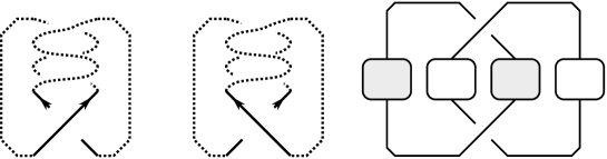
Figure 5. (i) The diagram $D$; the component $L_{i}$ lies above of $L_{j}$, except at $c$. (ii) The height-split $D_{-}$ by crossing change at $c$. (iii) Diagram $D^{\prime}$ which is ‘almost’ split.

∎

This observation leads to the following estimate of the lowest coefficient of the Conway polynomial.

Proposition 4.11.

When $L$ is a non-split prime weakly positive link, then

$$a_{\#L-1}(L)\geq lk(L)\geq\#L$$

unless $L$ is the Hopf link. (Here $lk(L)=\sum_{i<j}lk(L_{i},L_{j})$ is the total linking number.)

Proof.

By Lemma 4.10, the non-weighted linking graph $\Lambda(L^{\prime})$ has no isthmus. Then the assertion follows from (4.2) that $a_{\#L-1}$ is the number of spanning trees of $\Lambda^{\prime}(L)$, together with the standard fact of graph theory that a (loop-free multi-)graph without an isthmus has at least as many spanning trees as edges (and at least as many edges as vertices).

∎

As a complementary result, we mention the following.

Proposition 4.12.

If a non-split weakly positive link $L$ satisfies $a_{\#L-1}(L)=1$, then $L$ is the connected sum of $\#L-1$ Hopf links and some other (weakly positive) knots.

Proof.

We prove the assertion by induction on $\#L$. The case $\#L=2$ is proven in Proposition 4.11. By Hoste-Hosokawa’s formula (4.1), the linking graph $\Lambda(L)$ is the path graph with $\#L$ vertices and all the $(\#L-1)$ edges have weight one. In particular, by Lemma 4.10 $L$ is a connected sum of the Hopf link $H$ and some other weakly positive links $L^{\prime},L^{\prime\prime}$. Since $1=a_{\#L-1}(L)=a_{\#L^{\prime}-1}(L^{\prime})a_{1}(H)a_{\#L^{\prime\prime}-1}(L^{\prime\prime})$, we have $a_{\#L^{\prime}-1}(L^{\prime})=a_{\#L^{\prime\prime}-1}(L^{\prime\prime})=1$. Thus by induction both $L^{\prime}$ and $L^{\prime\prime}$ are a connected sum of Hopf links and some other (weakly positive) knots. ∎

Remark 4.13.

In the proof of Theorem 4.5, Lemma 4.6, Lemma 4.10 and Proposition 4.11, we only used the property that $G_{D}$ contains no sub-Gauss diagram of the form  .

5. Weakly successively almost positive diagram

In this section we introduce our main object, a weakly successively almost positive diagram, which is an obvious generalization of a successively almost positive diagram.

5.1. Weakly successively almost positive diagram and its standard skein triple

Definition 5.1.

We say that a diagram $D$ is weakly successively $k$-almost positive if all but $k$ crossings of $D$ are positive, and the $k$ negative crossings appear (but not necessarily consecutively) along a single overarc (see Figure 6). We call this the negative overarc.

Figure 6. Weakly successively almost positive diagram.

A weakly successively almost positive diagram is weakly positive. We take the ordering of the component so that the component that contains the negative overarc is the smallest (say, $L_{1}$), and take a base point $\ast_{1}$ near the initial point of the negative overarc. (The other choices, the orderings and base points on other components are arbitrary.)

In the following, we will always regard a weakly successively almost positive diagram as an ordered based link diagram, so that it is a weakly positive diagram.

The first underarc positive crossing of a weakly successively almost positive diagram $D$ is the positive crossing $c$ which we first pass along underarc; that is, the positive crossing which is the endpoint of the negative overarc (see Figure 7).

Definition 5.2 (Complexity).

For a weakly successively almost positive diagram $D$, we define the complexity of $D$ by

$$\mathcal{C}(D)=(c(D),c(D)-\ell(D))$$

where $\ell(D)$ is the number of crossings that lie on the negative overarc, which we call the length of the negative overarc.

For a weakly successively almost positive link $L$, we define the complexity

$$\mathcal{C}(L)=\min\{\mathcal{C}(D)\>|\>D\mbox{ is a weakly successively almost positive diagram of }L\}$$

We say that a successively almost diagram diagram $D$ of a link $L$ is minimum if $\mathcal{C}(D)=\mathcal{C}(L)$.

As usual, we compare the complexity according to the lexicographical ordering.

A key feature of a weakly successively almost positive diagram is that it admits a complexity-reducing skein resolution in the realm of weakly successively almost positive diagrams.

Definition 5.3.

Let $(D=D_{+},D_{0},D_{-})$ be the skein triple obtained at the first positive crossing $c$ terminating the negative overarc (which passes it as undercrossing). That is, $D_{0}$ is a diagram obtained by smoothing the crossing $c$, and $D_{-}$ is a diagram obtained by changing the positive crossing $c$ into a negative crossing.

We call $(D=D_{+},D_{0},D_{-})$ (or, the links $(L=L_{+},L_{0},L_{-})$ represented by $D$, $D_{0}$ and $D_{-}$) the standard skein triple of $D$.

Theorem 5.4.

Let $D$ be a weakly successively almost positive diagram and let $(D=D_{+},D_{-},D_{0})$ be the standard skein triple. Then both $D_{-}$ and $D_{0}$ are weakly successively almost positive and $\mathcal{C}(D_{0}),\mathcal{C}(D_{-})<\mathcal{C}(D)$.

Proof.

The digram $D_{-}$ is naturally regarded as a ordered based link diagram. We view $D_{0}$ as an ordered based link diagram as follows (see Figure 7).

When smoothing the crossing $c$ connects two distinct components $L_{1}$ and $L_{i}$ to form a component $L_{1^{*}}$ of $L_{0}$, then we just forget the relevant information of the component $L_{i}$; the ordering is $1^{*}<2<\cdots$ and the base point of $D_{1^{*}}$ is just $\ast_{1}$.

When the smoothing the crossing separates the component $L_{1}$ into two distinct components $L_{1^{\prime}}$ and $L_{1^{\prime\prime}}$, then we put the ordering $1^{\prime}<1^{\prime\prime}<2<\cdots$, where $L_{1^{\prime}}$ is the component that contains the base point $\ast_{1}$ of $D_{1}$. We take the base point $\ast_{1^{\prime}}$ of $D_{1^{\prime}}$ as $\ast_{1}$, and take a base point of $D_{1^{\prime\prime}}$ arbitrary (however, it is often convenient to take near the smoothed crossing $c$).

Figure 7. The first underarc crossing (left) of $D$ and how to view the diagram $D_{0}$ as a based ordered diagram (right)

Then both $D_{0}$ and $D_{-}$ are weakly successively positive. By the definition of the complexity, $\mathcal{C}(D_{0}),\mathcal{C}(D_{-})<\mathcal{C}(D)$. ∎

5.2. Split links in the standard skein triple

To use the standard skein triple effectively, we often need to take care of split links. Thanks to Theorem 4.5, we can completely understand when $L_{-}$ or $L_{0}$ becomes a split link, when we use the standard skein triple for a minimum w.s.a.p. diagram.

Lemma 5.5.

Let $D$ be a minimum weakly successively almost positive diagram representing a non-split link $L$, and let $(L=L_{+},L_{0},L_{-})$ be the standard skein triple of $L$. Then $L_{0}$ is always non-split. Moreover, if $L_{-}$ is split, then the minimum diagram $D$ can be taken so that is it of the form $D=D^{\prime}\#H\#D^{\prime\prime}$ (see Figure 8), where $D^{\prime}$ is a weakly successively almost positive diagram, $D^{\prime\prime}$ is a positive diagram, and $H$ is the standard Hopf link diagram.

Figure 8. Diagram $D=D^{\prime}\#H\#D^{\prime\prime}$

Proof.

Since $D$ is minimum, $D$ is reduced and the diagram $D_{0}$ is non-split.

First, assume to the contrary that $L_{0}$ is split. By Theorem 4.5, $D_{0}$ is height-split so $D_{0}=D_{u}\cup D_{s}$ where $D_{o}$ contains the negative overarc, lying above of $D_{u}$. Since the diagram $D_{0}$ itself is non-split, there are crossings between $D_{o}$ and $D_{u}$. However, as $D_{u}$ lies above of $D_{o}$, such a crossing can be removed by suitable isotopy. This leads to a weak successively almost positive diagram of $L$ with smaller complexity (see Figure 9). This is a contradiction.

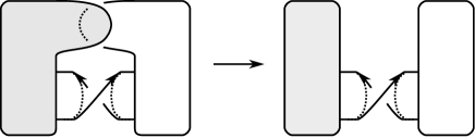
Figure 9. When $D_{0}$ is height-split, $D_{o}$ and $D_{u}$ overlap but their overlaps can be removed without touching the skein crossing $c$.

Next assume that $L_{-}$ is split. By Theorem 4.5, $D_{-}$ is height-split so we may write $D_{0}=D_{u}\cup D_{s}$ where $D_{o}$ contains the negative overarc, lying above of $D_{u}$. Since $D_{-}$ is not split, there are crossings between $D_{o}$ and $D_{u}$. The assumption that $D$ is minimum implies that the number of crossings between $D_{o}$ and $D_{u}$ is two. Because otherwise, as in the $D_{0}$ case, by removing overlaps between $D_{o}$ and $D_{u}$ we can find a weakly successively positive diagram of $L$ with smaller complexity. Then finally we modify the diagram $D$ in the form $D^{\prime}\#H\#D^{\prime\prime}$, without changing the complexity (see Figure 10).

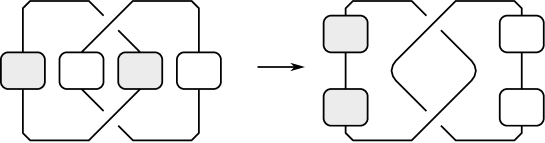
Figure 10. The case $D_{-}$ is height-split

∎

5.3. Standard unknotting/unlinking sequence

The standard skein triple gives rise to the following quite specific types of unknotting/unlinking sequence of a non-split w.s.a.p. link $L$.

Proposition-Definition 5.6 (Standard unknotting/unlinking sequence).

For each non-split w.s.a.p. link $L$, there exists a positive-to-negative crossing switch sequence

$$L=L_{0}\to L_{1}\to\cdots\to L_{m}$$ (5.1)

having the following properties:

• $L_{m}$ is the connected sum of $(\#L-1)$ positive Hopf links (when $L$ is a knot, $L_{m}$ is the unknot).

• All $L_{i}$ are non-split weakly successively almost positive.

• For each $i$, the crossing change $L_{i}\to L_{i+1}$ is realized as the standard skein triple $(D=D_{+},D_{-},D_{0})$ of a minimum weakly successively almost positive diagram $D$ of $L_{i}$.

We call such a crossing change sequence (5.1) a standard unknotting/unlinking sequence of $L$.

Proof.

To show the assertion, it is sufficient to show that for a non-split w.s.a.p. link $L$ which is not a connected sum of positive Hopf links, there is a minimum w.s.a.p. diagram $D$ of $L$ such that its standard resolution $D_{-}$ (the diagram $D_{-}$ in the standard skein triple $(D=D_{+},D_{0},D_{-})$) represents a non-split link.

By Lemma 5.5, $D_{-}$ represents a split link only if $D$ is a diagram connected sum $D=D^{\prime}\#H\#D^{\prime\prime}$, where $D^{\prime}$ is a w.s.a.p. diagram, $H$ is the standard Hopf link diagram, and $D^{\prime\prime}$ is a positive diagram. Let $L^{\prime}$ and $L^{\prime\prime}$ be the link represented by $D^{\prime}$ and $D^{\prime\prime}$, respectively.

If $L^{\prime}$ is not a connected sum of Hopf links, by induction there exists a minimum w.s.a.p. diagram $\widehat{D}^{\prime}$ of $L^{\prime}$ such that its standard resolution, $\widehat{D}^{\prime}_{-}$ does not represent a split link. Let $\widehat{D}=\widehat{D^{\prime}}\#H\#D^{\prime\prime}$, where the connected sum is taken away from the negative over arc of $\widehat{D}^{\prime}$. Then $\widehat{D}$ is a minimum w.s.a.p. diagram of $L$ and its standard resolution $\widehat{D_{-}}$ represents a non-split link.

If $L^{\prime}$ is a connected sum of Hopf links, $D^{\prime}$ is a positive diagram, and $L^{\prime\prime}$ is not a connected sum of Hopf links, then we replace the base point of $D$ on $D^{\prime\prime}$ to interchange the role of $D^{\prime}$ and $D^{\prime\prime}$. Then the same argument gives the desired minimum w.s.a.p. diagram $\widehat{D}$ of $L$. ∎

Remark 5.7.

Note that there is a way to modify the standard unknotting/unlinking sequence by choosing the standard skein triple not at the end of the negative overarc, but at the beginning. That is, we choose the crossing in $D_{+}$ to be the underpass terminating the overarc backwards, and in $D_{-}$ and $D_{0}$ can move the starting point along the negative overarc backward along its respective component. We will not need this freedom to extend the negative overarc backward too often, but this will be used for Theorem 9.8.

Remark 5.8.

It is informative to note that the argument in this section can be applied to a wider class of link diagrams. For the proofs of the theorems in this section to work, we actually need a class of diagrams $\mathcal{C}$ such that:

• The trivial link diagrams belong to the class $\mathcal{C}$.

• Theorem 4.5 holds; namely, a diagram $D$ in the class $\mathcal{C}$ represents a split link of and only if it is height-split.

• A minimum complexity diagram $D$ admits a positive skein resolution in the class $\mathcal{C}$; $D$ has a positive crossing $c$ such that in the skein triple $(D=D_{+},D_{0},D_{-})$, both $D_{-}$ and $D_{0}$ belong to the class $\mathcal{C}$.

In this prospect, a good feature of a weakly successively almost positive diagram is that the standard triple $(D=D_{+},D_{0},D_{-})$ satisfies the property (2).

Thus it an interesting problem to find a useful (and wider) class of diagrams $\mathcal{C}$ that satisfies all the above properties. Since the class of weakly positive diagrams satisfies properties (0) and (1), it is important to study to what extent we can expect the property (2) for weakly positive diagrams.

6. Application of standard skein triple I: Conway polynomial

We proceed to apply the standard skein triple to establish various properties of w.s.a.p. links.

For a general skein triple $(D=D_{+},D_{0},D_{-})$ of the diagram $D$, we always have the inequality

$$-\chi_{4}(D_{-})\geq-\chi_{4}(D)-2 -\chi_{4}(D_{0})\geq-\chi_{4}(D)-1$$ and . (6.1)

As for the maximum Euler characteristic, we can say much stronger.

Theorem 6.1 (Scharlemann-Thompson [ST]).

Let $(L_{+},L_{-},L_{0})$ be a skein triple. Then one of the following occurs.

• $\chi(L_{+})=\chi(L_{-})\leq\chi(L_{0})-1$.

• $\chi(L_{+})=\chi(L_{0})-1\leq\chi(L_{-})$.

• $\chi(L_{-})=\chi(L_{0})-1\leq\chi(L_{+})$.

As we will prove in Appendix, we can also say about the fiberedness properties from the skein triple.

Theorem 6.2 (Fibered link enhancement of Scharlemann-Thompson’s Theorem).

Let $(L_{+},L_{-},L_{0})$ be a skein triple.

• Assume that $\chi(L_{+})=\chi(L_{-})<\chi(L_{0})-1$, and that $L_{-}$ is fibered. Then $L_{+}$ is fibered.

• Assume that $\chi(L_{\pm})=\chi(L_{0})-1<\chi(L_{\mp})$, and that $L_{0}$ is fibered. Then $L_{\pm}$ is fibered.

Armed with this knowledge, we use the standard skein triple to relate knot polynomials and $\chi$ or $\chi_{4}$.

6.1. Conway polynomial and (4-ball) genus

The following property of the Conway polynomial nicely reflects the positivity of diagrams.

Definition 6.3.

We say that a Conway polynomial (see conventions of Section 2.7, specifically the form (2.7)) $\nabla_{L}(z)=\sum_{i=0}^{d}a_{\#L-1+2i}(L)z^{\#L-1+2i}$ is strictly positive if for all $i=0,\ldots,d$, we have $a_{\#L-1+2i}(L)>0$.

Theorem 6.4.

Assume $L$ is a non-split weakly successively almost positive link.

• $\displaystyle a_{\#L-1+2i}(L)\geq\binom{g_{4}(L)}{i}$.

• $\max\deg_{z}\nabla_{L}(z)=1-\chi(L)$.

• The Conway polynomial is strictly positive.

• $L$ is fibered if and only if the Conway polynomial is monic, i.e., its leading coefficient $a_{1-\chi(L)}(L)=1$.

This is an advance even when restricting to (almost) positive links. Property (iii) is only a slight improvement of [Cr, Corollary 2.2], but is (for almost positive links) subsumed by property (i), which was not known except in special cases. (See Corollary 6.5 and remarks below it for positive links, and Proposition 2.20 together with (2.14) for almost positive.) Further note that, while for a positive link properties (ii) and (iv) are rather clear (as discussed in [Cr]), part (ii) was obtained for an almost positive link in [St8] only with great effort, and part (iv) has remained a question there even in this case.

Proof.

All the assertions (i)–(iv) are proven by induction on the complexity of $L$. Let $D=D_{+}$ be a minimum w.s.a.p. diagram of $L$, and $(D_{+},D_{0},D_{-})$ be its standard skein triple.

Case 1. $L_{-}$ is split.

By Lemma 5.5, we may assume that the diagram $D$ is of the form $D=D^{\prime}\#H\#D^{\prime\prime}$ (where $D^{\prime}$ is w.s.a.p., $H$ is the standard Hopf link diagram, and $D^{\prime\prime}$ is positive).

Let $L^{\prime}$ and $L^{\prime\prime}$ be the links represented by $D^{\prime}$ and $D^{\prime\prime}$, respectively. Then

$$\#L=\#L^{\prime}+\#L^{\prime\prime},\quad g_{4}(L)\leq g_{4}(L^{\prime})+g_{4}(L^{\prime\prime}),\mbox{ and }\chi(L)=\chi(L^{\prime})+\chi(L^{\prime\prime})-2.$$

Moreover both $L^{\prime}$ and $L^{\prime\prime}$ have strictly smaller complexity so they satisfy the properties (i)–(iv).

Since $\nabla_{L}(z)=\nabla_{L^{\prime}}(z)\nabla_{H}(z)\nabla_{L^{\prime\prime}}(z)=z\nabla_{L^{\prime}}(z)\nabla_{L^{\prime\prime}}(z)$, the property (ii) of $L^{\prime}$ and $L^{\prime\prime}$ shows that

$$a_{\#L-1+2i}(L) =\sum_{k+j=i}a_{\#L^{\prime}-1+2j}(L^{\prime})a_{\#L^{\prime\prime}-1+2k}(L^{\prime\prime})$$

$$\geq\sum_{k+j=i}\binom{g_{4}(L^{\prime})}{j}\binom{g_{4}(L^{\prime\prime})}{k}=\binom{g_{4}(L^{\prime})+g_{4}(L^{\prime\prime})}{i}$$

$$\geq\binom{g_{4}(L)}{i}.$$

Similarly,

$$\max\deg_{z}\nabla_{L}(z) =\max\deg_{z}\nabla_{L^{\prime}}(z)+\max\deg_{z}\nabla_{L^{\prime\prime}}(z)+1$$

$$=(1-\chi(L^{\prime}))+(1-\chi(L^{\prime\prime}))+1$$

$$=1-(\chi(L^{\prime})+\chi(L^{\prime\prime})-2)$$

$$=1-\chi(L)$$

In particular, since

$$a_{\#L-1+2i}(L)=\sum_{k+j=i}a_{\#L^{\prime}-1+2j}(L^{\prime})a_{\#L^{\prime\prime}-1+2k}(L^{\prime\prime})\,,$$

this means that $a_{\#L-1+2i}(L)>0$ for all $i=0,\ldots,2g(L)=1-\chi(L)+1-\#L$.

Finally, if $\nabla_{L}(z)$ is monic, then $\nabla_{L^{\prime}}(z)$ and $\nabla_{L^{\prime\prime}}(z)$ are monic. By induction, $L^{\prime}$ and $L^{\prime\prime}$ are fibered, so $L=L^{\prime}\#H\#L^{\prime\prime}$ is fibered.

Case 2. $L_{-}$ is non-split.

To prove the assertion (i), we look at $\#L_{0}$. If $\#L_{0}=\#L-1$, then

$$g_{4}(D_{0})=(-\chi_{4}(D_{0})-\#L_{0}+2)/2\geq(-\chi_{4}(D)-1-(\#L-1)+2)/2=g_{4}(D).$$

Thus by induction and the skein relation,

$$a_{\#L-1+2i}(L)\geq a_{\#L_{0}-1+2i}(L_{0})\geq\binom{g_{4}(D_{0})}{i}=\binom{g_{4}(D)}{i}$$

Similarly, if $\#L_{0}=\#L+1$, then

$$g_{4}(D_{0})=(-\chi_{4}(D_{0})-\#L_{0}+2)/2\geq(-\chi_{4}(D)-1-(\#L+1)+2)/2=g_{4}(D)-1$$

and

$$g_{4}(D_{-})=(-\chi_{4}(D_{-})-\#L_{0}+2)/2\geq(-\chi_{4}(D)-2-\#L+2)/2=g_{4}(D)-1.$$

By induction and the skein relation, we get

$$a_{\#L-1+2i}(L) =a_{\#L_{0}-1+2(i-1)}(L_{0})+a_{\#L_{-}-1+2i}(L_{-})$$

$$\geq\binom{g_{4}(D)-1}{i-1}+\binom{g_{4}(D)-1}{i}=\binom{g_{4}(D)}{i}.$$

Similarly, to prove the assertion (ii)–(iv), we look at the maximal degree of the Conway polynomial. Since both $\nabla_{L_{0}}(z),\nabla_{L_{-}}(z)$ are strictly positive by induction, we consider the following three cases.

Case A: $\max\deg_{z}\nabla_{L}(z)=\max\deg_{z}\nabla_{L_{-}}(z)=\max\deg_{z}\nabla_{L_{0}}(z)+1$

In this case $\chi(L_{-})=\chi(L_{0})-1$, hence by Theorem 6.1, $\chi(L_{-})=\chi(L_{0})-1\leq\chi(L)$. Therefore

$$1-\chi(L)\leq 1-\chi(L_{-})=\max\deg_{z}\nabla_{L_{-}}(z)=\max\deg_{z}\nabla_{L}(z)\leq 1-\chi(L)\,,$$

so we get the desired equality $1-\chi(L)=\max\deg_{z}\nabla_{L}(z)$.

The strict positivity of $\nabla_{L}(z)$ follows from the strict positivity of $\nabla_{L_{-}}(z)$. In this case $\nabla_{L}(z)$ cannot be monic.

Case B: $\max\deg_{z}\nabla_{L}(z)=\max\deg_{z}\nabla_{L_{-}}(z)>\max\deg_{z}\nabla_{L_{0}}(z)+1$

Since $\chi(L_{-})=1-\max\deg_{z}\nabla_{L_{-}}(z)<1-\max\deg_{z}\nabla_{L_{0}}(z)=\chi(L_{0})-1$, we have by Theorem 6.1 $\chi(L_{+})=\chi(L_{-})<\chi(L_{0})-1$. Therefore, $1-\chi(L)=1-\chi(L_{-})=\max\deg_{z}\nabla_{L_{-}}(z)=\max\deg_{z}\nabla_{L}(z)$.

The strict positivity of $\nabla_{L}(z)$ follows from the strict positivity of $\nabla_{L_{-}}(z)$.

If $\nabla_{L}(z)$ is monic, then $\nabla_{L_{-}}(z)$ is monic, so by induction $L_{-}$ is fibered. By Theorem 6.2, we conclude $L$ is fibered.

Case C: $\max\deg_{z}\nabla_{L}(z)=\max\deg_{z}\nabla_{L_{0}}(z)+1>\max\deg_{z}\nabla_{L_{-}}(z)$

Since $\chi(L_{0})-1=-\max\deg_{z}\nabla_{L_{0}}(z)=1-\max\deg_{z}\nabla_{L}(z)<1-\max\deg_{z}\nabla_{L_{-}}(z)$, by Theorem 6.1 $\chi(L_{0})-1=\chi(L)<\chi(L_{-})$. Therefore, $1-\chi(L)=2-\chi(L_{0})=1+\max\deg_{z}\nabla_{L_{0}}(z)=\max\deg_{z}\nabla_{L}(z)$.

To see $\nabla_{L}(z)$ is strictly positive, we note that by Corollary 4.9

$$\min\deg_{z}\nabla_{L_{0}}(z)=\#L_{0}-1=\#L-2\mbox{ or, }\#L.$$

Thus for $i>0$, $\#L-1+2i\geq\#L_{0}-1$. Therefore for $i=0,\ldots,\frac{1}{2}(\max\deg_{z}\nabla_{L}(z)-\#L+1)$,

$$a_{\#L-1+2i}(L)=a_{\#L_{0}+2i}(L_{0})+a_{\#L_{-}-1+2i}(L_{-})\geq\begin{cases}a_{\#L-1}(L_{-})>0&(i=0)\\ a_{\#L-1+2i}(L_{0})>0&(i>0)\end{cases}$$

If $\nabla_{L}(z)$ is monic, then $\nabla_{L_{0}}(z)$ is monic, so by induction, $L_{0}$ is fibered. From Theorem 6.2, we conclude $L$ is fibered.

∎

Corollary 6.5.

If $K$ is a positive knot,

$$a_{2i}(K)\geq\binom{g(K)}{i}$$ (6.2)

This is an (ostensible) improvement of [St12, Proposition 4.1].

Example 6.6.

Using a similar (but simpler) induction argument, Van Buskirk [Bu] showed

$$\binom{g(K)}{i}\leq a_{2i}(K)\leq\binom{g(K)+i}{g(K)-i}$$ (6.3)

for a positive braid knot $K$.

While Corollary 6.5 extends the left estimate of (6.3) for positive knots, notice that no upper bound based on $g(K)$ and $i$ alone could apply for a general positive knot $K$, as the example of twist knots shows. Even for a fibered positive knot $K$ (of which there are finitely many for given $g(K)$), the right estimate in (6.3) is false in this form, as show the simple examples $K=10_{154},10_{161}$.

By Proposition 2.20, we have (6.2) for almost positive knots as well. In light of these results, we expect that in Theorem 6.4 (i) we can use $g(L)$ instead of $g_{4}(L)$. This is obviously true if (2.14) holds. We will address this issue at some length in [IS].

It is then interesting and natural to discuss to what extent Theorem 6.4 (i) or Corollary 6.5 is optimal.

The following examples and observations on other related results show the (limited) scope of (possible) further improvements. This pertains to some kind of optimality of Theorem 6.4 (i), at least as far as positive links are concerned.

Example 6.7.

1. The connected sums of (positive) Hopf links and trefoils make (6.2) exact for arbitrary $\#L,i$. Thus without adding further assumptions such as primeness, the bound (6.2) is optimal.

2. For the leading coefficient case, $i=g$, the presence of fibered links makes (6.2) exact in a trivial way, even though we add an assumption that $L$ is prime. Positive prime fibered links occur for all $g>0$ and $\#L$, as exemplify the (positively oriented) Montesinos links

   $$L=N_{m,k}=M\Bigl{(}-1,-\mbox{\small$\displaystyle\frac{1}{2k-1}$},\underbrace{\mbox{\small$\displaystyle\frac{1}{2}$},\dots,\mbox{\small$\displaystyle\frac{1}{2}$}}_{m}\Bigr{)}$$

   (for $k,m>0$, with $\#N_{m,k}=m$ and $g(N_{m,k})=k$ for (2.2); see [St7, Section 2.7] for explanation and convention). The most economic positive braid prime links we found occur as closures of extensions of the braids $\bigl{(}(\sigma_{1}\sigma_{3}\dots)(\sigma_{2}^{2}\sigma_{4}^{2}\dots)\bigr{)}^{2}$, which would apply approximately for all $g\geq\#L/2$.

3. For the second leading coefficient $i=g-1$, we mention that in [It2] we made some improvements of (6.3) for the prime positive braid link cases. For example, (6.3) tells that $g(K)\leq a_{2g-2}(K)(\leq 2g(K)-1)$ for a positive braid knot $K$, but it turns out that $a_{2g-2}(K)=2g(K)-1$ whenever $K$ is a prime positive braid knot. We have a similar improvement for $a_{2g(K)-4}$ whenever $K$ is prime.

4. If one considers $i<\!\!<g$, a simple skein (module) calculation for the (positively oriented) Montesinos links

   $$M_{m,n}=M\bigl{(}\underbrace{\raisebox{1.99997pt}{\small$2$}\!/\!\raisebox{-1.99997pt}{\small$3$},\dots,\raisebox{1.99997pt}{\small$2$}\!/\!\raisebox{-1.99997pt}{\small$3$}}_{n},\underbrace{\raisebox{1.99997pt}{\small$1$}\!/\!\raisebox{-1.99997pt}{\small$2$},\dots,\raisebox{1.99997pt}{\small$1$}\!/\!\raisebox{-1.99997pt}{\small$2$}}_{m}\bigr{)}$$

   (for $m>0$, with $\#M_{m,n}=m$ and $g(M_{m,n})=n$ for (2.2)) shows

   $$a_{m-1+2i}(M_{m,n})=\binom{n}{i}\cdot(m+i)\,.$$ (6.4)

   (For example, $n=2$ and $m=1$ gives $M_{1,2}=8_{15}$ with $\nabla(8_{15})=1+4z^{2}+3z^{4}$.) Thus, even if we consider prime links $L$, at least when $\#L$ and $i$ are fixed, (6.2) cannot be improved by more than the factor $\#L+i$ independent of $g$.

5. For $i=1$, and $K$ a positive knot, a substantial study was conducted in [St2]. Along with $a_{2}(K)\geq g(K)$ ([St2, Theorem 6.2]), we knew some modifications and improvements.

6. For $i=0$, the impact of $\#L$ under primeness, suggested by part 4), is indeed widely present in a much weaker setting. As we have seen in Proposition 4.11, for a weakly positive prime link, which is not the Hopf link, $a_{\#L-1}\geq\#L$. However, Theorem 6.4 only shows that $a_{\#L-1}\geq 1$.

On the other hand, the next example shows that Theorem 6.4 cannot be extended for 2-almost positive links.

Example 6.8.

The 2-almost positive knot $12_{1581}$ has $\max\deg\nabla<2g=4$. The 2-almost positive knot $13_{6407}$ has $\max\deg\nabla=2g=4$ and $\nabla$ is monic, but the knot is not fibered. This can be inspected from [St13].

The knots also fail various conditions on the HOMFLY polynomial which we prove in the next section. There is thus further evidence that even for $k=2$ most properties are lost, as soon as the “coordination” of the negative crossings is abandoned.

Finally, since the notion of successively almost positive link comes from a study of generalized torsion element, which is motivated from the bi-orderability of the link group, it deserves to mention the following corollary.

Corollary 6.9.

If $L$ is weakly successively almost positive, then the link group $\pi_{1}(S^{3}\setminus L)$ is not bi-orderable.

Proof.

Since $\nabla_{L}(z)$ is strictly positive, the Alexander polynomial $\Delta_{L}(t)=\nabla_{L}(t^{\frac{1}{2}}-t^{-\frac{1}{2}})$ cannot have a positive real root. Since for a link $L$ whose link group is bi-orderable, if $\max\deg_{z}\nabla_{L}(z)=1-\chi(L)$ (such a link is called rationally homologically fibered), then its Alexander polynomial $\Delta_{L}(t)$ has at least one positive real root [It1], this shows that $\pi_{1}(S^{3}\setminus L)$ is not bi-orderable.

∎

6.2. Unknotting number and the Conway polynomial

From the standard unknotting/unlinking sequence, we can also relate the unknotting/unlinking numbers and the Conway polynomial. We refer to Section 2.10.

Proposition 6.10.

• For each w.s.a.p. knot $K$,

  $$u(K)\leq u_{+}(K)\leq a_{2}(K)\,.$$ (6.5)

  Moreover, if $u(K)=a_{2}(K)$ or $u_{+}(K)=a_{2}(L)$, then the length of the standard unknotting sequence (5.1) is equal to $u(K)$, and $a_{2}(K_{i})=u(K)-i$.

• For each non-split link $L$,

  $$sp(L) \leq\#L-2+a_{\#L-1}(L)$$

  $$u^{comp}(L) \leq a_{\#L+1}(L)$$

  $$u(L) \leq\#L-2+a_{\#L-1}(L)+a_{\#L+1}(L)$$

Remark 6.11.

The inequality (6.5) was known for positive knots $K$ from [St2, Theorem 6.2]. More precisely, it can be seen from the proof (compare also with [St2, Theorem 6.4]) that $a_{2}(K)\geq u(D)$ for the unknotting number of a positive diagram $D$ of $K$. Since obviously such a diagram, we have $u_{+}(K)\leq u(D)$, this gives, for positive knots, a (slight) improvement of (6.5), not recovered here. However, in Corollary 9.10 we will have another (slight, but also independent) improvement of (6.5), valid for all w.s.a.p. knots $K$.

The inequality (6.5) for $a_{2}(K)=1$ would imply $u(K)=u_{+}(K)=1$, but in fact the case turns out uninteresting, because from Proposition 9.3 we will know exactly what knots occur: only the trefoil. (This is also the reason we chose in Example 6.12 a knot with $a_{2}=2$.)

Proof.

(i) Let $K=K_{0}\to K_{1}\to\cdots\to K_{m}=\bigcirc\,$ be a standard unknotting sequence. Since each crossing change $K_{i}\to K_{i+1}$ is a part of the standard skein triple $(D_{+},D_{0},D_{-})$ of a minimum w.s.a.p. diagram $D=D_{+}$ of $K_{i}$, by Lemma 5.5 the 2-component link $K^{\prime}_{i}$ represented by $D_{0}$ is not split. Thus $a_{1}(K^{\prime}_{i})\geq 1$. Therefore

$$a_{2}(K) =a_{2}(K_{1})+a_{1}(K^{\prime}_{0})=a_{2}(K_{2})+a_{1}(K^{\prime}_{1})+a_{1}(K^{\prime}_{0})$$

$$=\cdots$$

$$=a_{2}(K_{m})+\sum_{i=0}^{m-1}a_{1}(K^{\prime}_{m})=\sum_{i=0}^{m-1}a_{1}(K^{\prime}_{m})\geq m$$

In particular, when $a_{2}(K)=u(K)$ or $a_{2}(K)=u_{+}(L)$, this implies that the length $m=a_{2}(K)$ and $a_{2}(K_{i})=u(K)-i$.

(ii) For a standard unlinking sequence $L=L_{0}\to L_{1}\to\cdots\to L_{m}$ each crossing change $L_{i}\to L_{i+1}$ is a part of the standard skein triple $(D_{+},D_{-},D_{0})$ of a minimum w.s.a.p. diagram $D=D_{+}$ of $L_{i}$. By Lemma 5.5 the link $L^{\prime}_{i}$ represented by $D_{0}$ is not split.

When the crossing change $L_{i}\to L_{i+1}$ is a self-crossing change (the two strands at the crossing belong to the same component of $L_{i}$), then $\#L^{\prime}_{i}=\#L+1$. Therefore $a_{\#L}(L_{i}^{\prime})=a_{\#L_{i}^{\prime}-1}(L^{\prime}_{i})\geq 1$, and thus

$$a_{\#L-1}(L_{i}) =a_{\#L-1}(L_{i+1}),$$

$$a_{\#L+1}(L_{i}) =a_{\#L+1}(L_{i+1})+a_{\#L}(L^{\prime}_{i})\geq a_{\#L+1}(L_{i+1})+1$$

Similarly, when the crossing change $L_{i}\to L_{i+1}$ is a non-self-crossing change (the two strands at the crossing belong to different components of $L_{i}$), then $\#L^{\prime}_{i}=\#L-1$. Thus $a_{\#L-2}(L^{\prime}_{i})=a_{\#L_{i}^{\prime}-1}(L^{\prime}_{i})\geq 1$ and therefore

$$a_{\#L-1}(L_{i}) =a_{\#L-1}(L_{i+1})+a_{\#L-2}(L^{\prime}_{i})\geq a_{\#L-1}(L_{i+1})+1.$$

$$a_{\#L+1}(L_{i}) =a_{\#L+1}(L_{i+1})+a_{\#L}(L^{\prime}_{i})\geq a_{\#L+1}(L_{i+1})$$

Thus if in the standard unknotting sequence, there are $m^{\prime}$ self-crossing changes and $m^{\prime\prime}$ non-self-crossing changes, we have

$$a_{\#L-1}(L)\geq m^{\prime\prime}+1,\ a_{\#L+1}(L)\geq m^{\prime}$$

Since the link $L_{m}$, the connected sum of $(\#L-1)$ Hopf links, is made into the $\#L$-component unlink by $\#L-1$ non-self crossing changes, we have $m^{\prime}+m^{\prime\prime}+\#L-1\geq u(L)$. Moreover, since each component of $L_{m}$ is already the unknot,

$$m^{\prime\prime}+\#L-1\geq sp(L),\quad m^{\prime}\geq u^{comp}(L)$$

Therefore, we conclude

$$sp(L) \leq \#L-2+a_{\#L-1}(L),$$

$$u^{comp}(L) \leq a_{\#L+1}(L),$$

$$u(L) \leq \#L-2+a_{\#L-1}(L)+a_{\#L+1}(L)\,.$$

∎

Example 6.12.

The knot $K=11_{500}$ is a fibered knot with positive monic Conway polynomial $\nabla_{K}(z)=1+2z^{2}+2z^{4}+4z^{6}+z^{8}$, $g_{4}(K)=2$ and $u(K)=3$ (see [LMo]). Thus the knot satisfies all the properties in Theorem 6.4, but is not w.s.a.p. by Proposition 6.10.

Similarly, a standard unlinking sequence provides various lower inequalities.

Proposition 6.13.

If $L$ is a non-split w.s.a.p. link, then

$$\min\deg_{z}\nabla_{L}(z)=\#L-1\leq\sigma(L)\leq\max\deg_{z}\nabla_{L}(z)$$

Proof.

From a standard unlinking sequence (5.1), by positive-to-negative crossing changes, we may convert $L$ into a connected sum of $\#L-1$ (positive) Hopf links $L_{m}$, so $\sigma(L)\geq\sigma(L_{m})=\#L-1$.

For every link $L$, by [GiLv, Corollary 2.2]

$$|\sigma(L)|+1-\#L+m_{1}/2\leq m_{2}$$

where $m_{1}$ is the multiplicity of $-1$ as a root of the Alexander polynomial $\Delta_{L}(t)=\nabla(t^{\frac{1}{2}}-t^{-\frac{1}{2}})$, and $m_{2}$ is the number of roots of $\Delta_{L}(t)$ (counted with multiplicity) away from $1$. We have

$$m_{1}\geq 0\quad\mbox{and}$$

$$m_{2}\leq\max\deg_{z}\nabla_{L}(z)-\min\deg_{z}\nabla_{L}(z)\,.$$

Since $\sigma(L)\geq 0$ and $\#L-1=\min\deg_{z}\nabla_{L}(z)$ for a w.s.a.p. link $L$, this implies

$$\sigma(L)\leq\#L-1+(\max\deg_{z}\nabla_{L}(z)-\min\deg_{z}\nabla_{L}(z))=\max\deg_{z}\nabla_{L}(z)$$

∎

7. Application of standard skein triple II: HOMFLY polynomial

A similar argument proves various special properties of the HOMFLY polynomial. For the HOMFLY polynomials, we can often drop the assumption that $L$ is non-split, although we can often say more if we assume the non-splitness.

Theorem 7.1.

Assume $L$ is a weakly successively almost positive link. Then the HOMFLY polynomial

$$P_{K}(v,z)=\sum_{i,j}c_{i,j}v^{i}z^{j}$$

has the following properties.

• The coefficients $c_{i,j}$ satisfy the following.

  • $c_{i,j}=0$ if $i<j$.

  • $c_{j,j}\geq 0$ for all $j$.

  • $\sum_{i}c_{i,i}=1$. Thus $c_{j,j}=0$ for all $j$ except exactly one $j$, where $c_{j,j}=1$.

  • If $L$ is non-split, $c_{i,1-\chi(L)}\geq 0$ for all $i$.

  • $L$ is fibered if and only if $c_{i,1-\chi(L)}=0$ for all $i$ except exactly one $i$, where $c_{i,1-\chi(L)}=1$.

• $\max\deg_{z}P_{L}(v,z)=1-\chi(L)$.

• If $L$ is non-split, then $\min\deg_{v}P(L)\geq\#L-1$. Moreover, if $L$ is a non-trivial knot, then $\min\deg_{v}P(L)\geq 2$.

Proof.

The proof is similar to the Conway polynomial case and is done by induction on the complexity of $L$. Let $D$ be a minimum weakly successively positive diagram of $L$, and let $(D=D_{+},D_{0},D_{-})$ be the the standard skein triple.

(i-a), (i-b): They follow from the skein relation

$$P_{L}(v,z)=v^{2}P_{L_{-}}(v,z)+vzP_{L_{0}}(v,z).$$

(i-c): It follows from the identity

$$P(v,v^{-1}-v)=1\,.$$ (7.1)

Indeed, this implies

$$1 =P(v,v^{-1}-v)=\sum_{i\geq j}c_{i,j}v^{i}(v^{-1}-v)^{j}=\sum_{j}c_{j,j}+(\mbox{terms of degree}>0\mbox{ in }v).$$

(i-d): The assertion is easy to see if $L_{-}$ is non-split. If $L_{-}$ is split, then by Lemma 5.5 $L$ is a connected sum $L^{\prime}\#H\#L^{\prime\prime}$ where $L^{\prime},L^{\prime\prime}$ are non-split weakly successively almost positive links of smaller complexity and $H$ is the positive Hopf link. The HOMFLY polynomial of the positive Hopf link $H$ is $P_{H}(v,z)=z^{-1}(v-v^{3})+vz$ hence $H$ satisfies (i-d). By induction, both $L^{\prime}$ and $L^{\prime\prime}$ satisfy (i-d) and $P_{L}(v,z)=P_{L^{\prime}}(v,z)P_{H}(v,z)P_{L^{\prime\prime}}(v,z)$, thus we conclude that $L$ also satisfies (i-d).

(i-e): It follows from (i-d) and the observation that $a_{1-\chi(L)}(L)=\sum_{i}c_{i,1-\chi(L)}$.

(ii): The proof for the non-split link case is the same as for the Conway polynomial case. Assume thus that $L$ is a split link, hence $L$ is a split union of non-split links $L=L_{1}\sqcup\cdots\sqcup L_{m}$. (That is, $L_{i}$ are the split components of $L$.) Thus $1-\chi(L_{i})=\max\deg_{z}P_{L_{i}}(v,z)$. Since $P_{L}(v,z)=\left(\frac{v^{-1}-v}{z}\right)^{m-1}P_{L_{1}}(v,z)\cdots P_{L_{m}}(v,z)$ we conclude

$$1-\chi(L) =1-(\chi(L_{1})+\cdots+\chi(L_{m}))$$

$$=(1-m)+(1-\chi(L_{1}))+\cdots+(1-\chi(L_{m}))$$

$$=(1-m)+\max\deg_{z}P_{L_{1}}(v,z)+\cdots+\max\deg_{z}P_{L_{1}}(v,z)$$

$$=\max\deg_{z}P_{L}(v,z).$$

(iii): The first assertion is obviously true for connected sums of (positive) Hopf links (meant to include the unknot if $\#L=1$), so the standard unknotting/unlinking sequence and the induction over the complexity prove the first assertion.

For a non-trivial knot $K$ let $(K=K_{+},K_{0},K_{-})$ be the standard skein triple. Since $K_{0}$ is a non-split 2-component link, $\min\deg_{v}P_{K_{0}}(v,z)\geq 1$. Thus from the skein relation

$$P_{K}(v,z)=vzP_{K_{0}}(v,z)+v^{2}P_{K_{-}}(v,z)$$

we conclude $\min\deg_{v}P_{K}(v,z)\geq 2$.

∎

As an application, we show that an alternating (or, more generally homogeneous) w.s.a.p. link is always a positive link.

Corollary 7.2.

A homogeneous link $L$ is weakly successively almost positive if and only if it is positive.

Proof.

It is sufficient to show the case $L$ is non-split. We show that if a diagram $D$ of $L$ is a Murasugi sum of a positive diagram $D_{+}$ and a non-trivial negative diagram $D_{-}$, then the link represented by $D$ is never weakly successively almost positive.

Let $L_{+}$ and $L_{-}$ be the links represented by $D_{+}$ and $D_{-}$, respectively. (Note that $\chi(L_{\pm})=\chi(D_{\pm})$.) By [Cr] (or use Theorem 8.1 (iii) ),

$$c_{1-\chi(L_{+}),1-\chi(L_{+})}(L_{+})\neq 0\,.$$

Similarly, since the mirror image of a negative diagram is a positive diagram, there exists a $j<1-\chi(L_{-})$ with $c_{j,1-\chi(L_{-})}(L_{-})\neq 0$, for example, $j=\chi(L_{-})-1$; see (2.4).

By Theorem 2.10 (i), (iii), this implies that there is a $j^{\prime}<1-\chi(L)$ with $c_{j^{\prime},1-\chi(L)}(L)\neq 0$. Therefore, by Theorem 7.1 (i-a), $L$ is not w.s.a.p. ∎

As for the assertion (i-e) in Theorem 7.1, for the positive link case this single non-zero $c_{i,1-\chi(L)}$ is $c_{1-\chi(L),1-\chi(L)}$ [Cr], so we expect the following.

Conjecture 7.3.

For a fibered weakly successively almost positive link $L$, the unique non-zero coefficient $c_{i,1-\chi(L)}$ in (i-e) is $c_{1-\chi(L),1-\chi(L)}=1$.

The HOMFLY polynomial remains very powerful in ruling out the w.s.a.p. property. The difficulties to circumvent it in finding essential applications of other tests lead to rather complicated knots in, and outside, the tables.

This will become evident at many places, like Examples 9.4, 9.16, 6.12, and 9.6. We chose not to do a search for bizarre instances throughout, and neither do we have space to discuss how such examples were gathered. But they clearly emphasize both the strength of the HOMFLY polynomial and the value of practical computation.

Since the Jones polynomial is recovered from the HOMFLY polynomial, as a consequence we get the following properties of the Jones polynomial.

Theorem 7.4.

Let $L$ be a weakly successively almost positive link, and let $V_{L}(t)$ be its Jones polynomial.

• The sign of the coefficient $t^{\min\deg_{t}V_{L}(t)}$ is $(-1)^{\#L-1}$.

• $\min\deg_{v}P_{K}(v,z)\leq 2\min\deg_{t}V_{K}(t)\leq\max\deg_{z}P_{K}(v,z)=1-\chi(K)$

• If $L$ is non-trivial and non-split, $\min\deg_{t}V_{K}(t)\geq\begin{cases}1&(\#L=1)\\ \frac{\#L-1}{2}&(\#L>1).\end{cases}$

Proof.

Let $P_{L}(v,z)=\sum_{i,j}c_{i,j}v^{i}z^{j}$ be the HOMFLY polynomial of $L$, and let

$$m=\min\Bigl{\{}\frac{1}{2}(2i-j)\>|\>c_{i,j}\neq 0\Bigr{\}}\,.$$ (7.2)

Since

$$V_{L}(t)=P_{L}(t,t^{1/2}-t^{-1/2})=\sum_{i\geq j}c_{i,j}t^{i}(t^{1/2}-t^{-1/2})^{j}\,,$$

$$\min\deg_{t}V_{L}(t) =\min\deg_{t}P_{L}(t,t^{1/2}-t^{-1/2})\geq m$$ (7.3)

Since $P_{L}(v,z)\in(vz)^{1-\#L}\mathbb{Z}[v^{\pm 2},z^{2}]$, the equality happens when the coefficients $c_{i,j}$ satisfy the property

$$c_{i,j}>0\mbox{ whenever }\frac{1}{2}(2i-j)=m$$ (7.4)

Now thanks to the skein relation $P_{L}(v,z)=v^{2}P_{L_{-}}(v,z)+vzP_{L_{0}}(v,z)$, the property (7.4) holds for $L$ when it holds for both $L_{-}$ and $L_{0}$. Since the HOMFLY polynomial of the unlink satisfies the property (7.4), we conclude that

$$\min\deg_{t}V_{L}(t)=m$$

holds for all weakly successively positive links.

Since $c_{i,j}>0$ in (7.4), their sum is also positive, meaning that the coefficient of $t^{m}$ in $V_{L}(t)$ is positive (resp. negative) if even (resp. odd) powers of $v$ occur in $P_{L}(v,z)$, which is equivalent to $\#L$ being odd (resp. even). Note that the sign comes from the $-$ for $t^{-1/2}$ in (7.3). This shows (i).

Consider (ii). By Theorem 7.1 (i-c), there is an $i_{0}=j_{0}$ with $c_{i_{0},j_{0}}\neq 0$. In (7.2), this gives $2i-j=j_{0}$, and therefore we conclude

$$m\leq\frac{1}{2}j_{0}\leq\frac{1}{2}\max\deg_{z}P_{L}(v,z)\,.$$

Then, by Theorem 7.1 (i-a), we have in (7.2) that $i\geq j$, so that $2i-j\geq i$, and we conclude

$$m\geq\frac{1}{2}\min\deg_{v}P_{L}(v,z)\,.$$

This proves (ii). Finally, (iii) similarly easily follows from (ii) and Theorem 7.1 (iii). ∎

8. Link polynomials for Bennequin-sharp weakly successively almost positive links

The results on link polynomials of weakly successively almost positive links can be improved if we further assume that $L$ is Bennequin-sharp.

Theorem 8.1.

Let $L$ be a weakly successively almost positive link. If $L$ is Bennequin-sharp, then the following holds.

• $\displaystyle a_{\#L-1+2i}(L)\geq\binom{g(L)}{i}$.

• $\min\deg_{v}P_{L}(v,z)=2\min\deg_{t}V_{L}(t)=\max\deg_{z}P_{L}(v,z)=1-\chi(L)$.

• For $j\neq 1-\chi(L)$, $c_{j,j}=0$, unless $j=1-\chi(L)$. Furthermore, $c_{1-\chi(L),1-\chi(L)}=1$.

• If $L$ is non-split, then $c_{1-\chi(L),-1-\chi(L)}\leq 1-\chi(L)$. Equality holds when $L$ is fibered.

• If $L$ is non-split, then

  $$V_{L}(t) =(-1)^{\#L-1}\Bigl{(}t^{\frac{1}{2}(1-\chi(L))}+\bigl{(}\chi(L)-1+c_{1-\chi(L),-1-\chi(L)}\bigr{)}t^{\frac{1}{2}(3-\chi(L))}$$

  $$\quad+(\mbox{higher degree terms})\Bigr{)}.$$

  In particular, if $L$ is fibered then

  $$V_{L}(t)=(-1)^{\#L-1}t^{\frac{1}{2}(1-\chi(L))}+\bigl{(}\mbox{terms of $t$-degree at least $\frac{1}{2}(5-\chi(L))$}\bigr{)}$$

Proof.

(i): It follows from Proposition 2.15 and Theorem 6.4 (i).

(ii): Since $L$ is Bennequin-sharp, by Proposition 2.15

$$1-\chi(L)=\overline{sl}(L)+1\leq\min\deg_{v}P_{L}(v,z)$$

where the second inequality is Morton’s inequality [Mo]. Thus by Theorem 7.4 (ii),

$$1-\chi(L)\leq\min\deg_{v}P_{L}(v,z)\leq 2\min\deg_{t}V_{L}(t)\leq\max\deg_{z}P_{L}(v,z)=1-\chi(L).$$

(iii): By (ii) and Theorem 7.1 (i-a) $c_{i,i}=0$ unless $i\neq 1-\chi(L)$, hence By Theorem 7.1 (i-c), $c_{1-\chi(L),1-\chi(L)}=1$.

(iv): By looking at the coefficient of $v^{2}$ in $P_{K}(v,v^{-1}-v)=1$ we get

$$-(1-\chi(L))c_{1-\chi(L),1-\chi(L)}+c_{3-\chi(L),1-\chi(L)}+c_{1-\chi(L),-1-\chi(L)}=0$$

Thus if $L$ is non-split, by Theorem 7.1 (i-d)

$$(1-\chi(L))-c_{1-\chi(L),-1-\chi(L)}=c_{3-\chi(L),1-\chi(L)}\geq 0$$ (8.1)

as desired. Moreover, when $L$ is fibered (in this case $L$ is automatically non-split), the Conway polynomial $\nabla_{L}(z)=P_{K}(1,z)$ is monic. By (iii)

$$1=a_{1-\chi(L)}(L)=\sum_{j\geq 1-\chi(L)}c_{j,1-\chi(L)}=1+\sum_{j>1-\chi(L)}c_{j,1-\chi(L)}.$$

Since $c_{j,1-\chi(L)}\geq 0$ by Theorem 7.1 (i-d), this implies that $c_{j,1-\chi(L)}=0$ for all $j>1-\chi(L)$. Therefore

$$(1-\chi(L))-c_{1-\chi(L),-1-\chi(L)}=c_{3-\chi(L),1-\chi(L)}=0.$$

(v): Since $V_{L}(t)=P_{L}(t,t^{1/2}-t^{-1/2})=\sum_{i\geq j}c_{i,j}t^{i}(t^{1/2}-t^{-1/2})^{j}$, we immediately get

$$V_{L}(t) =(-1)^{1-\chi(L)}\left(t^{\frac{1}{2}(1-\chi(L))}+(-1+\chi(L)+c_{1-\chi(L),-1-\chi(L)})t^{\frac{3}{2}(3-\chi(L))}+\cdots\right)$$

∎

Remark 8.2.

It is known that when $L$ is a positive link, then the Theorem 8.1 (iv),(v) is an equivalence [St10]; $c_{1-\chi(L),-1-\chi(L)}=1-\chi(L)$ (equivalently, the coefficient of $t^{\frac{1}{2}(3-\chi(L))}$ is zero) if and only if $L$ is fibered.

This equivalence can be extended to Bennequin-sharp weakly successively almost positive links, if one can show the following gap-free property of the maximal $z$-degree term of $P_{L}(v,z)$;

$$c_{i,1-\chi(L)}\neq 0,c_{j,1-\chi(L)}\neq 0\Rightarrow c_{k,1-\chi(L)}\neq 0\mbox{ for all }k=i,i+2,\ldots,j$$ (8.2)

i.e., the coefficient of $z^{1-\chi(L)}$ is of the form

$$c_{m,1-\chi(L)}v^{m}+c_{m+2,1-\chi(L)}v^{m+2}+\cdots+c_{M,1-\chi(L)}v^{M}$$

for some $m,M$, where all the coefficients $c_{k,1-\chi(L)}$ are non-zero. Compare with Theorem 6.4 (iii), which can be understood as the assertion that the Conway polynomial of weakly successively almost positive link is gap-free.

Indeed, the inequality (8.1) in the proof of (iv) shows that $c_{1-\chi(L),-1-\chi(L)}=1-\chi(L)$ if and only if $c_{3-\chi(L),1-\chi(L)}=0$.

When we assume that $P_{L}(v,z)$ satisfies the gap-free property (8.2), $c_{3-\chi(L),1-\chi(L)}=0$ means that $c_{m,1-\chi(L)}=0$ for all $m\geq 3-\chi(L)$. Therefore

$$a_{1-\chi(L)}(L)=\sum_{i}c_{i,1-\chi(L)}=c_{1-\chi(L),1-\chi(L)}=1\,.$$

By Theorem 6.4 (iv), $L$ is fibered.

We mention that because of Proposition 2.20, Theorem 8.1 (ii) positively answers [St3, Question 2].

Corollary 8.3.

If $L$ is almost positive link,

$$\min\deg_{v}P_{L}(v,z)=\max\deg_{z}P_{L}(v,z)=1-\chi(L)$$

9. Positivity of the signature and related invariants

It is known that the signature of a non-trivial (almost) positive link is always strictly positive: $\sigma(K)>0$ [PT]. In this section we extend the positivity of the signature to w.s.a.p. links and derive some consequences.

Since we have already seen $\sigma(L)\geq\#L-1$ in Proposition 6.13 for non-split links, it remains to consider the knot case.

Theorem 9.1.

If $K$ is a non-trivial weakly successively almost positive knot, then $\sigma(K)>0$. In particular $K$ is not (algebraically) slice, and is not amphicheiral.

Proof.

Let $\det(K)=|\nabla_{K}(2\sqrt{-1})|\geq 1$ be the determinant of the knot $K$ (compare with Section 2.10). Assume to the contrary that there is a non-trivial w.s.a.p. knot $K$ with $\sigma(K)=0$. Let

$$d=\min\{\det(K)\>|\>K\mbox{ is a non-trivial w.s.a.p.\ knot},\sigma(K)=0\},$$

and take a non-trivial w.s.a.p. knot $K$ with $\sigma(K)=0$ and $\det(K)=d$ so that among such knots, its complexity $\mathcal{C}(K)$ is minimum.

Let $D$ be a minimum w.s.a.p. diagram of $K$ and let $(D=D_{+},D_{0},D_{-})$ be the standard skein triple. Since $0=\sigma(K_{+})\geq\sigma(K_{-})\geq 0$, $\sigma(K_{-})=0$. By the minimum assumption of the complextiy of $K$, this implies that $\det(K_{-})>d$.

By Theorem 2.12 (v), $\sigma(K)=\sigma(K_{-})=0$ implies that $\nabla_{K}(2\sqrt{-1}),\nabla_{K_{-}}(2\sqrt{-1})>0$. Also, $K_{0}$ is w.s.a.p., so by Proposition 4.3, we have $\sigma(K_{0})\geq 0$. Thus from Theorem 2.12 (ii), we see that $\sigma(K)=\sigma(K_{-})=0$ implies $\sigma(K_{0})\in\{0,1\}$. Hence by Theorem 2.12 (v), $(2\sqrt{-1})\nabla_{K_{0}}(2\sqrt{-1})\geq 0$. Therefore

$$\det(K_{+}) =|\nabla_{K}(2\sqrt{-1})|=\nabla_{K}(2\sqrt{-1})=\nabla_{K_{-}}(2\sqrt{-1})+(2\sqrt{-1})\nabla_{K_{0}}(2\sqrt{-1})$$

$$=|\nabla_{K_{-}}(2\sqrt{-1})|+(2\sqrt{-1})\nabla_{K_{0}}(2\sqrt{-1})$$

$$\geq\det(K_{-})>d.$$

This is a contradiction. ∎

We give a few applications of this signature positivity.

First we give a characterization of the simplest w.s.a.p. links and knots.

Proposition 9.2.

For a w.s.a.p. link $L$, the following conditions are equivalent:

• $L$ is a connected sum of $\#L-1$ positive Hopf links.

• $\nabla_{L}(z)=z^{\#L-1}$.

• $a_{\#L-1}(L)=1$ and $\sigma(L)=\#L-1$.

Proof.

(i) implies (ii) and (iii). To see (ii) implies (iii), we note that $\nabla_{L}(z)=z^{\#L-1}$ implies that $L$ is non-split. Therefore $\sigma(L)\geq\#L-1$ by Proposition 4.11. If $\sigma(L)>\#L-1$, then by Corollary 6.13, $\nabla_{L}(z)\neq z^{\#L-1}$, so $\sigma(L)=\#L-1$.

We show (iii) implies (i). Again, $a_{\#L-1}(L)=1$ implies that $L$ is non-split, hence by Proposition 4.11, $L$ is a connected sum of $(\#L-1)$ positive Hopf links and some other w.s.a.p. knots. Since a non-trivial w.s.a.p. knot has non-trivial signature, $\sigma(L)=\#L-1$ implies that $L$ is a connected sum of $(\#L-1)$ positive Hopf link. ∎

Proposition 9.3.

A weakly successively almost positive knot $K$ is the positive (right-handed) trefoil if and only if $a_{2}(K)=1$.

This conclusion was also well-known for positive knots from [St2], thus Proposition 9.3 is its generalization.

Proof.

The one direction is obvious, so assume $a_{2}(K)=1$. Let $D$ be a minimum w.s.a.p. diagram of $K$ and let $(D_{+},D_{-},D_{0})$ be the standard skein triple. Since $K_{0}$ is not split, $a_{1}(K_{0})\geq 1$.

Since $a_{2}(K)=a_{2}(K_{-})+a_{1}(K_{0})=1$, we need that $a_{2}(K_{-})=0$ and $a_{1}(K_{0})=1$. This implies that $K_{-}$ is the unknot. Since $1\leq\sigma(K_{0})\leq\sigma(K_{-})+1=1$, this implies $\sigma(K_{0})=1$, so by Proposition 9.2, $K_{0}$ is the Hopf link. Thus $\nabla_{K}(z)=\nabla_{K_{-}}(z)+z\nabla_{K_{0}}(z)=1+z^{2}$. This shows that $K$ is a fibered knot of genus one, and only the trefoil is possible. ∎

Example 9.4.

The knots $16_{838974}$, $16_{954872}$ and $16_{1263307}$ are among (very) few that can be prohibited from being w.s.a.p. using Proposition 9.3 but not by the previous conditions on $\sigma$, $\nabla$ and $P$. (Composite knots can be discarded with Proposition 6.10 and Scharlemann’s result [Sch], and no smaller crossing prime examples exist.)

Next we give a slight improvement of the strictly positive property of the Conway polynomial in Theorem 6.4.

Proposition 9.5.

Let $L$ be a w.s.a.p. non-split link. Assume $a_{j}(L)=1$ for some $j>\#L-1$. Then $\max\deg_{z}\nabla(L)=j$ (hence $j=1-\chi(L)$ and $L$ is fibered).

Another way of saying this is that all “intermediate” coefficients of $\nabla$, those for $0<i<d=g(L)$ in (2.7), are at least $2$ for a non-split w.s.a.p. link $L$.

This will, of course, readily follow from Theorem 6.4 (i) if we are able to see $g(L)=g_{4}(L)$, which follows if $L$ is Bennequin-sharp by Proposition 2.15. But as long as this is not fully established (see Question 12.1 (a)(b)) the proposition retains an own (however modest) merit.

Proof.

We prove the assertion on the complexity of $L$. Let $D$ be a minimum w.s.a.p. diagram of $L$ and $(L_{+},L_{0},L_{-})$ be the standard skein triple. Since

$$1=a_{j}(L)=a_{j}(L_{-})+a_{j-1}(L_{0})$$

we have two cases.

Case 1. $a_{j-1}(L_{0})=0$ and $a_{j}(L_{-})=1$

By induction, $\max\deg_{z}\nabla_{L_{-}}(z)=j$, and $\max\deg_{z}\nabla_{L_{0}}(z)<j-1$. Hence $\max\deg_{z}\nabla_{L}(z)=j$ as desired.

Case 2. $a_{j}(L_{-})=0$ and $a_{j-1}(L_{0})=1$

By induction, $\max\deg_{z}\nabla_{L_{-}}(z)<j$. If $j-1>\#L_{0}-1$, then $\max\deg_{z}\nabla_{L_{0}}(z)=j-1$ by induction, so $\max\deg_{z}\nabla_{L}(z)=j$ as desired.

Thus we assume that $j-1=\#L_{0}-1$. Since $j>\#L-1$, this happens only if $j=\#L+1=\#L_{0}$.

If $\max\deg_{z}\nabla_{L_{0}}(z)=j-1=\#L_{0}-1$, then $\max\deg_{z}\nabla_{L}(z)=j$ as desired. So we may further assume that $\max\deg_{z}\nabla_{L_{0}}(z)>j-1=\#L_{0}-1$, namely, $\nabla_{L_{0}}(z)\neq z^{\#L_{0}-1}$.

By Proposition 4.12 and Proposition 9.2, $a_{\#L_{0}-1}(L_{0})=1$ and $\nabla_{L_{0}}(z)\neq z^{\#L_{0}-1}$ imply that $L_{0}$ is a connected sum of $(\#L_{0}-1)$ Hopf links and non-trivial w.s.a.p. knots. By Theorem 9.1, $\sigma(L_{0})\geq(\#L_{0}-1)+2=\#L+2$.

On the other hand, by Proposition 6.13

$$\#L_{-}-1\leq\sigma(L_{-})\leq\max\deg_{z}\nabla_{L_{-}}(z)<j=\#L_{-}+1\,,$$

which means that $\sigma(L_{-})\in\{\#L-1,\#L\}$. This is a contradiction, because $\sigma(L_{-})-\sigma(L_{0})\in\{-1,0,1\}$.

∎

Example 9.6.

The knots $14_{26091}$ and $14_{43602}$ satisfy $a_{2}>a_{4}=1$ and $\max\deg_{z}\nabla=6$, so by Proposition 9.5 they are not w.s.a.p. They are among minimal crossing prime knots which demonstrate that this criterion is more essential compared to Example 9.4.

Note that Proposition 9.5 implies that for a w.s.a.p. knot $K$,

$$\nabla_{K}(1)=\Delta_{K}\left(\mbox{\small$\displaystyle\frac{3\pm\sqrt{5}}{2}$}\right)=\sum_{i=1}^{g(K)}a_{2i}(K)\geq 2g(K)$$ (9.1)

Equality is possible only if $K$ is fibered, and we know yet no examples except $K=3_{1}$ and $3_{1}\#3_{1}$. Indeed, (9.1) looks to be far from optimal since it follows from Theorem 6.4 (i)

$$\nabla_{K}(1)=\Delta_{K}\left(\mbox{\small$\displaystyle\frac{3\pm\sqrt{5}}{2}$}\right)=\sum_{i=1}^{g(K)}a_{2i}(K)\,\geq\,\sum_{i=1}^{g(K)}\binom{2g_{4}(K)}{i}=2^{g_{4}(K)}\geq 2^{\sigma(K)/2}$$ (9.2)

Finally, we give a slightly different characterization of the trefoil and the unknot.

A knot $K$ is 2-trivadjacent (2-adjacent to the trivial knot) if $K$ admits a diagram $D$ having two distinct crossings $c_{1},c_{2}$ such that when we apply the crossing change at $c_{1},c_{2}$, or both $c_{1}$ and $c_{2}$, we get the unknot (see [AK] for the notion of adjacency).

Corollary 9.7.

A weakly successively almost positive knot is 2-trivadjacent if and only if it is either the unknot or the trefoil.

Proof.

Assume that $K$ is non-trivial and 2-trivadjacent, so there is a diagram $D$ with crossings $c_{1},c_{2}$ such that crossing change at $c_{1},c_{2}$, or both $c_{1}$ and $c_{2}$ yields the unknot (note that $D$ may not be w.s.a.p.).

By Theorem 9.1 $\sigma(K)>0$. Since negative-to-positive crossing change never decreases the signature, this means that both $c_{1}$ and $c_{2}$ are positive crossings.

For $\ast_{1},\ast_{2}\in\{+,-,0\}$, let $D_{\ast_{1},\ast_{2}}$ be the diagram obtained by replacing each $\ast_{i}$ as positive/negative/smoothed crossing (so $D=D_{++}$). By the skein formula of the Conway polynomial, for every diagram $D$ we have

$$z^{2}\nabla_{D_{00}}(z) =\left(\nabla_{D_{++}}(z)-\nabla_{D_{-+}}(z)-\nabla_{D_{+-}}(z)+\nabla_{D_{--}}(z)\right).$$

Since $D_{+-},D_{-+},D_{--}$ represents the unknot, we get $\nabla_{K}(z)=1+z^{2}\nabla_{D_{00}}(z)$. This implies $a_{2}(K)=0,1$.

If $a_{2}(K)=0$, then $K$ is the unknot by Theorem 6.4 (iii) and (ii). If $a_{2}(K)=1$, then $K$ is the trefoil by Proposition 9.3. ∎

This observation allows us to extend strict positivity for various other invariants. The following theorem is a generalization of the result for almost positive knots [PT, Theorem 1.4].

Theorem 9.8.

Let $K$ be a weakly successively almost positive knot. Then by positive-to-negative crossing changes, $K$ can be made to the trefoil knot, $d_{+}(K,3_{1})<\infty$.

Proof.

Let $D$ be a minimum complexity w.s.a.p. diagram of $K$. We prove the theorem by induction on the complexity $\mathcal{C}$. Let $c_{1}$ and $c_{2}$ be the positive crossings which are the end points of the negative overarc. Note that $c_{1}\neq c_{2}$, since $K$ does have a Hopf link factor. Since crossing changes at $c_{1}$ or $c_{2}$ give rise to w.s.a.p. diagrams of knots with smaller complexity (Remark 5.7), if the crossing change at $c_{1}$ or $c_{2}$ gives a non-trivial knot $\tilde{K}$, then by induction on $\tilde{K}$, we find a positive-to-negative crossing change sequence which makes $K$ to the trefoil.

Thus we assume that both crossing changes, at $c_{1}$ or $c_{2}$, give rise to the unknot, i.e., $K_{-+}=K_{+-}=\bigcirc$. Let $K_{--}$ be the w.s.a.p. knot obtained by crossing changes at both $c_{1}$ and $c_{2}$. Since the signature cannot increase by the positive to negative crossing change, $\sigma(K_{--})=0$ which means that $K_{--}$ is also the unknot. Therefore $K$ is $2$-trivadjacent. By Corollary 9.7, this means that $K$ is the trefoil. ∎

This gives more positivity properties, such as,

Corollary 9.9.

If $K$ is a non-trivial w.s.a.p. knot, then $\tau(K)\geq 1$.

The following is a useful remark on the proof of Theorem 9.8. It improves Proposition 6.10 (i).

Corollary 9.10.

If $K$ is a (non-trivial) w.s.a.p. knot, then $K$ has (positive-to-negative) Gordian distance $d_{+}(K,3_{1})\leq a_{2}(K)-1$ to the (positive) trefoil.

Proof.

Obviously we constructed in the proof of Theorem 9.8 a standard unknotting sequence, so that $K_{m-1}$ is the trefoil, and $m\leq a_{2}(K)$. ∎

To see that Corollary 9.10 is useful as a w.s.a.p. test, consider the following examples.

$$\begin{array}[]{cc}\includegraphics*[width=156.49014pt]{eps/17_115227.eps}&\includegraphics*[width=156.49014pt]{eps/18_176710.eps}\\ 17_{*115227}&18_{*176710}\\[22.76219pt] \includegraphics*[width=156.49014pt]{eps/19_405610.eps}&\includegraphics*[width=156.49014pt]{eps/19_393831.eps}\\ 19_{*405610}&19_{*393831}\end{array}$$

Figure 11. Knots used in the construction of Example 9.12 and 9.13, showing that Corollary 9.10 can be essential as a test for w.s.a.p. All these knots also satisfy the property (a)–(d) stated in Example 9.11.

Example 9.11.

Take a knot $K$ having the following properties (there are systematic constructions of such knots for any such $\nabla$ [St6, Theorem 3.1]).

• $u(K)=1$ and $\sigma(K)=2$.

• $\nabla_{K}(z)$ is strictly positive and $a_{2}(K)=1$.

• $\det(K)=|\nabla(2\sqrt{-1})|\equiv 3\bmod 4$ but is not $3$.

• $g(K)=\max\deg_{z}\nabla_{K}(z)$, and $K$ is fibered if $\nabla_{K}(z)$ is monic.

Then the knot

$$K_{n}^{*}=\#^{n}K$$

has $\sigma(K_{n}^{*})>0$ and its Conway polynomial satisfies all the properties of a w.s.a.p. link which we proved so far.

On the other hand, by Proposition 2.22, $d(K_{n}^{*},3_{1})\geq n$. Since $a_{2}(K_{n}^{*})=u(K_{n}^{*})=n$, by Corollary 9.10 $K_{n}^{*}$ is not w.s.a.p. for all $n>1$.

The knot $K=10_{156}$ is the simplest example of such a knot.

We have $10_{156}\not\geq 3_{1}$, because for $\omega=e^{2\pi\sqrt{-1}t}$ for $\frac{1}{3}<t<\alpha$ (here $e^{2\pi\sqrt{-1}\alpha}$ is a root of the Alexander polynomial of $10_{156}$), $\sigma_{\omega}(3_{1})=2>0=\sigma_{\omega}(10_{156})$.

The knot $K=14_{28430}$ is another example satisfying all the required properties, where $d_{+}(K,3_{1})=1$. So $d_{+}(K^{*}_{n},3_{1})\leq n$. But we have no strict inequality; this can be seen either with Proposition 2.22, or by using Levine-Tristram signatures.

Example 9.12.

The construction of Example 9.11 does not control the HOMFLY polynomial and (like at several other places) it turned out that among table knots, the HOMFLY test (Theorem 7.1) could not be overcome in examples with provable $u\leq a_{2}$. However, $K^{*}_{n}$ for $K$ being the 17 crossing knot $K=17_{*115227}$ does the job. (Also $\tau(K)=1$, so that Corollary 9.9 cannot be used either.)

For any of the (at least 9 provably distinct) examples $K$ we could not confirm that $K\geq 3_{1}$ (for one example, this was ruled out using Levine-Tristram signatures, and the other 8 are undecided).

Example 9.13.

To construct examples $K_{n}^{*}\geq 3_{1}$ making the HOMFLY obstruction fail, we have to use connected sums with different factors. (And again the restrictivity of the test manifests itself in rather complicated knots, which required a lot of effort to put together.)

The knot $K=19_{*405610}$ has $\tau=1$, $\sigma=2$, $u_{+}=1$, $\nabla=1+z^{2}+2z^{4}+z^{6}$ (so $\det=35$). Similarly, the knot $K=18_{*176710}$ has $\tau=1$, $\sigma=2$, $u_{+}=1$, $\nabla=1+z^{2}-z^{4}+2z^{6}$ (so $\det=147$), and $d_{+}(K,3_{1})=1$.

Let

$$K_{n}^{*}=18_{*176710}\#\,\left(\#^{n-1}19_{*405610}\right).$$

By Proposition 2.22

$$u_{+}(K_{n}^{*})=d_{+}(K_{n}^{*},3_{1})=a_{2}(K_{n}^{*})=n.$$ (9.3)

(So $d_{+}(K,3_{1})$ is the smallest possible for which Corollary 9.10 would obstruct.)

Also $\nabla(K_{n}^{*})$ is strictly positive for $n\geq 2$. Moreover, for $n\geq 3$ it also satisfies the property stated in Proposition 9.5.

For a different polynomial, instead of $18_{*176710}$, one can also take $19_{*393831}$ with $\nabla=1+z^{2}-4z^{4}+3z^{6}$, where $n\geq 4$ would work. (Only Proposition 2.22 for $\delta=7$ is applied so far to establish (9.3) in all examples we have.)

For a w.s.a.p. knot with $a_{2}(K)=u(K)$, we get the following more specific property.

Proposition 9.14.

Assume that $K$ is a w.s.a.p. knot of $\sigma(K)=2$. If $a_{2}(K)=u(K)$, then $\det(K)\leq 4a_{2}(K)-1$. Moreover, if equality occurs then $g(K)=1$.

Proof.

We prove the proposition by induction on $u(K)=a_{2}(K)$. If $u(K)=a_{2}(K)=1$, then $K$ is the trefoil, and the assertion follows. Thus in the following we assume that $u(K)=a_{2}(K)>1$.

Let $K=K_{0}\to K_{1}\to\cdots\to K_{u(K)-1}\to K_{u(K)}$ be a standard unknotting sequence. By Proposition 6.10 (i), $u(K_{1})=a_{2}(K_{1})=u(K)-1$ so by induction $\det(K_{1})\leq 4a_{2}(K_{1})-1$.

Since $2=\sigma(K)\geq\sigma(K_{1})>0$, $\sigma(K_{0})=\sigma(K_{1})=2$. Thus by Theorem 2.12 (v), $\det(K_{0})=-\nabla_{K_{0}}(2\sqrt{-1})$ and $\det(K_{1})=-\nabla_{K_{1}}(2\sqrt{-1})$.

Let $K^{\prime}$ be the (w.s.a.p.) 2-component link obtained by smoothing the crossing of $K=K_{0}$ where we apply the crossing change. Then $K^{\prime}$ is non-split, $a_{1}(K^{\prime})=1$, and $\sigma(K^{\prime})\in\{1,2,3\}$.

By Proposition 4.11, $a_{1}(K^{\prime})=1$ implies that either $K^{\prime}$ is the Hopf link, or, it is non-prime. If $K^{\prime}$ is non-prime we put $K^{\prime}=L_{1}\#L_{2}$, where $L_{1}$ is the 2-component w.s.a.p. link and $L_{2}$ is a w.s.a.p. knot. Since $\sigma(L_{1})\geq 1$ and $\sigma(L_{2})\geq 2$, $\sigma(K^{\prime})\geq 3$. Thus in this case $\sigma(K^{\prime})=3$. By Theorem 2.12 (vi), this implies that $(2\sqrt{-1})\nabla_{K^{\prime}}(2\sqrt{-1})>0$. Therefore

$$\det(K) =-\nabla_{K}(2\sqrt{-1})=-\nabla_{K_{1}}(2\sqrt{-1})-(2\sqrt{-1})\nabla_{K^{\prime}}(2\sqrt{-1})$$

$$<\det(K_{1})\leq 4a_{2}(K_{1})-1\leq 4a_{2}(K)-1$$

In particular, the inequality is strict.

If $K^{\prime}$ is the Hopf link,

$$\det(K) =-\nabla_{K}(2\sqrt{-1})=-\nabla_{K_{1}}(2\sqrt{-1})-(2\sqrt{-1})\nabla_{K^{\prime}}(2\sqrt{-1})$$

$$=\det(K_{1})+4\leq 4a_{2}(K_{1})-1+4=4a_{2}(K)-1$$

In this case, the inequality is exact, i.e.,

$$\det(K)=4a_{2}(K)-1$$ (9.4)

holds if and only if $\det(K_{1})=4a_{2}(K_{1})-1$. By induction $g(K_{1})=1$, hence $\nabla_{K_{1}}(z)=1+a_{2}(K_{1})z^{2}$. We conclude that if (9.4) holds then $\nabla_{K}(z)=\nabla_{K_{1}}(z)+z\nabla_{K^{\prime}}(z)=1+a_{2}(K)z^{2}$, so $g(K)=1$. ∎

Proposition 9.14 can be used to detect non-w.s.a.p. knots.

Example 9.15.

Some knots whose unknotting number was previously considered, as listed in [LMo], and to which the test applies (and $\nabla$ is strictly positive) are $10_{117}$, $11_{378}$, $11_{391}$, $11_{494}$, $3_{1}\#6_{3}$ (for unknotting number 2) and $12_{1435}$ (for unknotting number 3). For higher $a_{2}$ one can take $3_{1}\#\left(\#^{m-1}10_{164}\right)$ (whose unknotting number being equal to $a_{2}=m$ follows from Proposition 2.22 with $\delta=3$).

The HOMFLY polynomial easily prohibits these knots all from being w.s.a.p. as well. To obtain essential examples, i.e., such for which all previous conditions on $P$, $\nabla$ and $\sigma$ fail to rule out w.s.a.p., we have to enter more exotic territory.

Example 9.16.

The minimal crossing prime essential examples with $a_{2}(K)=u(K)=2$ are $K=15_{128571}$ and $15_{148331}$. Their unknotting number 2 is determined from the tau-invariant $\tau(K)=2$ (compare Section 2.8), or alternatively from Lickorish’s linking form test. They also have Gordian distance $1$ to the trefoil.

There is not enough scope of prime knot tables, resp. information about their entries, for us to offer a new instance for unknotting number 3. The simplest essential examples we could build for general unknotting number using connected sums are

$$3_{1}\#(\#^{m-1}16_{658907})\,,$$ (9.5)

using $a_{2}(16_{658907})=1$, $\sigma(16_{658907})=0$ and $\tau(16_{658907})=u(16_{658907})=1$. Such a composite knot obviously also has Gordian distance $m-1=a_{2}-1$ to the trefoil.

10. General signature estimate and concordance finiteness

As perhaps the most general known sharpening of $\sigma>0$ for a positive diagram $D$ of a link $L$, the stronger inequality

$$\sigma(L)\geq\frac{1}{24}(1-\chi(D))\;\;\left(=\frac{1}{24}(1-\chi(L))\right)$$ (10.1)

was proven in [BDL, Theorem 1.2].

Since a positive-to-negative crossing change decreases the signature by at most $2$, (10.1) implies

$$\sigma(L)\geq\frac{1}{24}(1-\chi(D))-2c_{-}(D)$$ (10.2)

for a general link diagram $D$.

In this section we give the following improvement of the signature estimate (10.2) and discuss its applications.

Theorem 10.1.

Let $D$ be a connected reduced diagram of a non-trivial link $L$. Then

$$\sigma(L)\geq\frac{1}{12}(1-\chi(D))-\frac{4}{3}c_{-}(D)+\frac{1}{2}\geq\frac{1}{12}(1-\chi(L))-\frac{4}{3}c_{-}(D)+\frac{1}{2}.$$ (10.3)

10.1. Proof of signature estimate

In large part, our proof of Theorem 10.1 goes along the same lines as Baader-Dehornoy-Liechti’s argument [BDL], adapted so that it can be applied to general link diagrams with slight improvements.

The proof is based on Gordon-Litherland’s theorem [GoLi]. For a (possibly non-orientable) spanning surface $F$ of a link $L$, let $\langle\;,\;\rangle_{F}:H_{1}(F)\times H_{1}(F)\rightarrow\mathbb{Z}$ be the Gordon-Litherland pairing of $F$; for $a,b\in H_{1}(F)$, let $\alpha,\beta$ be curves on $S$ that represent $a$, $b$, and let $p_{F}:\nu(F)\rightarrow F$ be the unit normal bundle of $F$. The Gordon-Litherland pairing of $a$ and $b$ is defined by $\langle a,b\rangle_{F}=lk(\alpha,p_{S}^{-1}(\beta))$.

For an oriented link $L$, the Gordon-Litherland theorem states

$$-\sigma(L)=\sigma(F)+\frac{1}{2}e(F,L).$$ (10.4)

Here $\sigma(F)$ is the signature of the Gordon-Litherland pairing of $F$, and

$$e(F,L)=-\frac{1}{2}\langle[L],[L]\rangle_{F}-lk(L)\,,$$

where $lk(L)=\sum_{i<j}lk(L_{i},L_{j})$ is the total linking number.

A checkerboard coloring assigns to regions two colors, black and white, so that at each crossing, its opposite regions receive the same color, and its neighbored ones opposite color. We fix one of the (two) checkerboard colorings of a diagram $D$, and let $B$ and $W$ be the black and white checkerboard surfaces.

We say that a crossing $c$ of $D$ is of type a (resp. of type b) if, when we put the overarc so that it is a horizontal line, the upper right-hand side and the lower left-hand side (resp. the lower right-hand side and the upper left-hand side) are colored by black (see Figure 12).

Similarly, we say that a crossing $c$ is of type I (resp. of type II) if the black region is compatible (resp. incompatible) with the orientation of the diagram (i.e., its Seifert circle regions are black resp. white; see Figure 12). In the definition of type a/b, the orientation of $D$ is irrelevant, whereas in the definition of type I/II, the over-under information is irrelevant.

We say that a crossing $c$ is of type $Ia$, for example, if $c$ is both of type I and of type a. We put $c_{Ia},c_{Ib},c_{IIa},c_{IIb}$ to be the number of crossings of type $Ia,Ib,IIa,IIb$, respectively. Note that a positive (resp. negative) crossing is either of type Ib or IIa (resp. Ia or IIb), so

$$c_{+}(D)=c_{Ib}+c_{IIa},\quad c_{-}(D)=c_{Ia}+c_{IIb}.$$ (10.5)

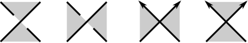
Figure 12. Types of crossings with respect to the checkerboard coloring

By the definition of the Gordon-Litherland pairing,

$$\frac{1}{2}e(B,L)=c_{IIb}-c_{IIa},\quad\frac{1}{2}e(W,L)=c_{Ia}-c_{Ib}.$$

Thus by (10.4) and (10.5)

$$-2\sigma(L)=\sigma(B)+\sigma(W)-c_{+}(D)+c_{-}(D)$$ (10.6)

Let $\mathcal{R}(W)$ and $\mathcal{R}(B)$ be the set of white and black regions, respectively. For a white region $R\in\mathcal{R}(W)$, we associate a simple closed curve $\gamma_{R}$ on $B$ which is a mild perturbation of the boundary of $R$ (see Figure 13).

We say that the region $R$ is of type $(\alpha,\beta)$ if $R$ contains $\alpha$ type a crossings and $\beta$ type b crossings as its corners. By definition,

$$\langle[\gamma_{R}],[\gamma_{R}]\rangle_{B}=\alpha-\beta$$

when $R$ is of type $(\alpha,\beta)$.

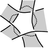
Figure 13. Curve $\gamma_{R}$ for a white region $R$

For a black region $R\in\mathcal{R}(B)$, the curve $\gamma_{R}$ on $W$ and the notion of type $(\alpha,\beta)$ are defined similarly, and the Gordon-Litherland pairing is given by

$$\langle[\gamma_{R}],[\gamma_{R}]\rangle_{W}=\beta-\alpha$$

when $R$ is of type $(\alpha,\beta)$.

Proof of Theorem 10.1.

Since $D$ is reduced, there are no regions of type $(1,0)$ or $(0,1)$. Moreover, since we assume that $L$ is non-trivial, $\#\mathcal{R}(W),\#\mathcal{R}(B)\geq 2$. (We use $\#$ henceforth for the cardinality of a set.)

Let $\Gamma$ be the planar graph whose vertices $V(\Gamma)$ are white regions of type $(\alpha,\beta)$ with $\alpha-\beta\leq 0$, and two vertices $R,R^{\prime}$ are connected by an edge if they share a corner. By Appel-Haken’s Four-Color Theorem [AH] there is a 4-coloring $col:V(\Gamma)\rightarrow\{1,2,3,4\}$; if two vertices $v,v^{\prime}$ are connected by an edge, then $col(v)\neq col(v^{\prime})$.

Let $\Gamma^{\prime}$ be the subgraph of $\Gamma$ such that $V(\Gamma^{\prime})=col^{-1}\{1,2\}$ and $E(\Gamma^{\prime})=\{e\in E(\Gamma)\>|\>e\mbox{ connects vertices }v,w\in V(\Gamma^{\prime})\}$. With no loss of generality, we assume that

$$\#V(\Gamma^{\prime})\geq\frac{1}{2}\#V(\Gamma).$$

Let $V_{B}$ be the subspace of $H_{1}(B)$ generated by $[\gamma_{R}]$ for $R\in V(\Gamma^{\prime})$. Since $\Gamma^{\prime}$ is bipartite, the restriction of the Gordon-Litherland pairing $\langle\;,\;\rangle_{B}$ on $V_{B}$ is of the form $\begin{pmatrix}D_{1}&X^{T}\\ X&D_{2}\end{pmatrix}$, where $D_{1},D_{2}$ are diagonal matrices with non-positive diagonals. Therefore the Gordon-Litherland pairing is non-positive on $V_{B}$.

Let $\gamma^{W}_{>0}$ be the number of white regions $R$ such that $\langle[\gamma_{R}],[\gamma_{R}]\rangle_{B}>0$.

If $V(\Gamma^{\prime})\neq\mathcal{R}(W)$, $\{[\gamma_{R}]\>|\>R\in V(\Gamma^{\prime})\}$ is a basis of $V_{B}$, so $\dim V_{B}=\#V(\Gamma^{\prime})$. Thus

$$\dim V_{B}=\#V(\Gamma^{\prime})\geq\frac{1}{2}\#V(\Gamma)=\frac{1}{2}(\#\mathcal{R}(W)-\gamma^{W}_{>0}).$$

If $V(\Gamma^{\prime})=\mathcal{R}(W)$, then $\dim V_{B}=\dim H_{1}(B)=\#\mathcal{R}(W)-1$. Since $\mathcal{R}(W)\geq 2$, we have the same lower bound

$$\dim V_{B}=\#\mathcal{R}(W)-1\geq\frac{1}{2}\#\mathcal{R}(W)\geq\frac{1}{2}(\#\mathcal{R}(W)-\gamma^{W}_{>0})$$

Therefore we get an upper bound

$$\sigma(B) \leq\dim H_{1}(B)-\dim V_{B}=(\#\mathcal{R}(W)-1)-\dim V_{B}$$

$$\leq\frac{1}{2}\#\mathcal{R}(W)-1+\frac{1}{2}\gamma^{W}_{>0}$$

By a parallel argument for the white surface $W$, we get a similar estimate

$$\sigma(W)\leq\frac{1}{2}\#\mathcal{R}(B)-1+\frac{1}{2}\gamma^{B}_{>0}\,,$$

where $\gamma^{B}_{>0}$ is the number of black regions $R$ such that $\langle[\gamma_{R}],[\gamma_{R}]\rangle_{W}>0$.

Since $\#\mathcal{R}(W)+\#\mathcal{R}(B)-2=c(D)$, by (10.6) we get

$$-2\sigma(K)\leq-\frac{1}{2}c(D)+2c_{-}(D)+\frac{1}{2}\gamma_{>0}^{B}+\frac{1}{2}\gamma_{>0}^{W}-1\,.$$ (10.7)

It remains to estimate $\gamma_{>0}^{B}+\gamma_{>0}^{W}$. Let $\gamma^{W}(\alpha,\beta)$ be the number of white regions of type $(\alpha,\beta)$. By definition of $\gamma^{W}_{>0}$,

$$\gamma^{W}_{>0}=\sum_{\begin{subarray}{c}\alpha>\beta\geq 0\\ \alpha\geq 2\end{subarray}}\gamma^{W}(\alpha,\beta).$$

By counting the number of the crossings of type $a$ that appear as a corner of white regions, we get

$$2(c_{Ia}+c_{IIa}) =\sum_{\alpha,\beta\geq 0}\alpha\gamma^{W}(\alpha,\beta)$$

$$\geq 2\gamma^{W}(2,0)+2\gamma^{W}(2,1)+3\sum_{\begin{subarray}{c}\alpha>\beta\geq 0\\ \alpha\geq 3\end{subarray}}\gamma^{W}(\alpha,\beta)$$

$$=-\gamma^{W}(2,0)-\gamma^{W}(2,1)+3\sum_{\begin{subarray}{c}\alpha>\beta\geq 0\\ \alpha\geq 2\end{subarray}}\gamma^{W}(\alpha,\beta)$$

$$=-\gamma^{W}(2,0)-\gamma^{W}(2,1)+3\gamma^{W}_{>0}.$$

Thus we conclude

$$\gamma^{W}_{>0}\leq\frac{2}{3}(c_{Ia}+c_{IIa})+\frac{1}{3}\gamma^{W}(2,0)+\frac{1}{3}\gamma^{W}(2,1)\,.$$ (10.8)

The same argument for the black regions shows

$$\gamma^{B}_{>0}\leq\frac{2}{3}(c_{Ib}+c_{IIb})+\frac{1}{3}\gamma^{B}(2,0)+\frac{1}{3}\gamma^{B}(2,1)\,,$$ (10.9)

where $\gamma^{B}(\alpha,\beta)$ is the number of black regions of type $(\alpha,\beta)$.

Recall that a positive crossing appears as either of type Ib or of type IIa. If the corner of a white region $R$ is a crossing of type IIa, then the orientation of the link and the orientation of the white region switch; in the language of Definition 2.3, the white region $R$ is a non-Seifert circle region near a crossing of type IIa.

Thus if all the corners of $R$ are positive crossings, then the region $R$ must be of type $(\alpha,2\beta^{\prime})$. In particular, if a white region $R$ is of type $(2,1)$, at least one of its corners is a negative crossing. Similarly, if a white region $R$ is of type $(2,0)$, its corners are either both positive, or both negative.

Let $\gamma^{W}_{\pm}(2,0)$ be the number of white regions of type $(2,0)$ whose corners are positive and negative crossings, respectively. By counting the number of negative crossings that appear as a corner of type $(2,1)$ regions or type $(2,0)$ regions we get

$$\gamma^{W}(2,1)+2\gamma^{W}_{-}(2,0)\leq 2c_{-}(D).$$

Thus

$$\gamma^{W}(2,1)+\gamma^{W}_{-}(2,0)\leq 2c_{-}(D).$$ (10.10)

Let $s_{W}(D)$ be the number of Seifert circles of $D$ which are the boundary of a white bigon such that both corners are positive crossings. When both corners of a white region $R$ of type $(2,0)$ are positive, then the boundary of $R$ forms a Seifert circle of $D$, so

$$\gamma^{W}_{+}(2,0)\leq s_{W}(D).$$

By the same argument we get the similar inequalities

$$\gamma^{B}(2,1)+\gamma^{B}_{-}(2,0)\leq 2c_{-}(D)\,,$$ (10.11)

and

$$\gamma^{B}_{+}(2,0)\leq s_{B}(D)\,,$$

where $\gamma^{B}_{\pm}(2,0)$ and $s_{B}(D)$ are defined similarly (with white regions/bigons replaced by black ones).

Since a Seifert circle cannot be the boundary of a white bigon and black bigon at the same time,

$$s_{W}(D)+s_{B}(D)\leq s(D).$$

The equality happens only if all the Seifert circles are bigons with positive crossings as their corners. Thus the equality occurs only if $D$ is the standard torus $(2,2n)$ link diagram (with opposite orientation, so that it bounds an annulus). In this case, the asserted inequality of the signature is obvious, so in the following we can assume the slightly stronger inequality

$$s_{W}(D)+s_{B}(D)\leq s(D)-1.$$

Therefore we get

$$\gamma^{W}_{+}(2,0)+\gamma^{B}_{+}(2,0)\leq s(D)-1\,.$$ (10.12)

Hence by (10.10), (10.11) and (10.12),

$$\gamma^{W}(2,0)+\gamma^{W}(2,1)+\gamma^{B}(2,0)+\gamma^{B}(2,1)$$

$$\quad=\gamma^{W}_{-}(2,0)+\gamma^{W}(2,1)+\gamma^{B}_{-}(2,0)+\gamma^{B}(2,1)+\gamma^{W}_{+}(2,0)+\gamma^{B}_{+}(2,0)$$

$$\quad\leq 4c_{-}(D)+s(D)-1.$$

By (10.7), (10.8) and (10.9) we conclude

$$-2\sigma(K) \leq-\frac{1}{2}c(D)+2c_{-}(D)+\frac{1}{2}\gamma_{>0}^{B}+\frac{1}{2}\gamma_{>0}^{W}-1$$

$$\leq-\frac{1}{2}c(D)+2c_{-}(D)+\frac{1}{3}(c_{Ia}+c_{IIa}+c_{Ib}+c_{IIb})$$

$$\quad\qquad+\frac{1}{6}(\gamma^{W}(2,0)+\gamma^{W}(2,1)+\gamma^{B}(2,0)+\gamma^{B}(2,1))-1$$

$$\leq-\frac{1}{2}c(D)+2c_{-}(D)+\frac{1}{3}c(D)+\frac{1}{6}(s(D)-1)+\frac{2}{3}c_{-}(D)-1$$

$$=\frac{1}{6}(s(D)-c(D)-1)+\frac{8}{3}c_{-}(D)-1.$$

∎

When $D$ is a successively $k$-almost positive diagram, some additional arguments give the following slightly better estimate.

Corollary 10.2.

If $K$ has a successively $k$-almost positive diagram $D$, then

$$\sigma(K)\geq\frac{1}{12}(1-\chi(D))-\frac{13}{12}k+\frac{1}{3}\,.$$

Proof of Corollary 10.2.

We show that when $D$ is a successively $k$-almost positive diagram, we have improvements of inequalities (10.10), (10.11) and (10.12), which appeared in the previous proof, leading to the better estimate as stated.

For a successively $k$-almost positive diagram, $\gamma^{W}_{-}(2,0)=0$. We have that $\gamma^{W}(2,1)$ is bounded above by the number of white regions which have at least one negative crossing as a corner, and the number of such white regions is at most $k+1$. Thus we get

$$\gamma^{W}_{-}(2,0)+\gamma^{W}(2,1)\leq k+1\ (=c_{-}(D)+1).$$ (10.10^′)

The same argument shows

$$\gamma^{B}_{-}(2,0)+\gamma^{B}(2,1)\leq k+1\ (=c_{-}(D)+1).$$ (10.11^′)

There are $(k+1)$ Seifert circles which are connected to a negative crossing. None of these Seifert circles is the boundary of a white or black bigon with positive corners, and therefore $s_{W}(D)+s_{B}(D)\leq s(D)-(k+1)$. Thus we have a better bound

$$\gamma^{W}_{+}(2,0)+\gamma^{B}_{+}(2,0)\leq s(D)-(k+1).$$ (10.12^′)

Using (10.10^′), (10.11^′), (10.12^′) instead of (10.10), (10.11), (10.12) we get

$$-2\sigma(K) \leq-\frac{1}{2}c(D)+2c_{-}(D)+\frac{1}{2}\gamma_{>0}^{B}+\frac{1}{2}\gamma_{>0}^{W}-1$$

$$\leq-\frac{1}{2}c(D)+2c_{-}(D)+\frac{1}{3}c(D)+\frac{1}{6}(s(D)-1)+\frac{1}{6}c_{-}(D)+\frac{1}{3}-1$$

$$=\frac{1}{6}(s(D)-c(D)-1)+\frac{13}{6}c_{-}(D)-\frac{2}{3}.$$

∎

10.2. Concordance finiteness

In [BDL, Theorem 1.1], as an application of the signature estimate, the authors showed that every topological knot concordance class contains finitely many positive knots. Since their arguments are based on the (Levine-Tristram) signatures, which are invariants of algebraic knot concordance, they actually showed the same finiteness result for an algebraic knot concordance class.

Theorem 10.1 and the non-negativity of the Levine-Tristram signature (proven in Proposition 4.3) lead to a more general concordance finiteness result.

Theorem 10.3.

For any $\varepsilon>0$ and $C\in\mathbb{R}$, every algebraic knot concordance class $\mathcal{K}$ contains only finitely many weakly successively $k_{i}$-almost positive knots $K_{i}$ such that

$$k_{i}\leq\Bigl{(}\frac{1}{8}-\varepsilon\Bigr{)}\cdot g_{c}(K_{i})+C\,.$$ (10.13)

Proof.

Assume, to the contrary, that the algebraic concordance class $\mathcal{K}$ contains infinitely many weakly successively $k_{i}$-almost positive knots $\{K_{i}\}$.

Let $D_{i}$ be a successively $k_{i}$-almost positive diagram of $K_{i}$. Since $g_{c}(K_{i})\leq g_{c}(D_{i})$, by the assumption (keeping $\varepsilon\leq\frac{1}{8}$)

$$k_{i}\leq\Bigl{(}\frac{1}{8}-\varepsilon\Bigr{)}\cdot g_{c}(K_{i})+C\leq\Bigl{(}\frac{1}{8}-\varepsilon\Bigr{)}\cdot g_{c}(D_{i})+C\,,$$

so we get

$$g_{c}(D_{i})-8k_{i}\geq 8\varepsilon g_{c}(D_{i})-8C.$$

By Theorem 10.1

$$\sigma(\mathcal{K})=\sigma(K_{i}) \geq\frac{1}{6}g(D_{i})-\frac{4}{3}k_{i}+\frac{1}{2}=\frac{1}{6}\left(g_{c}(D_{i})-8k_{i}\right)+\frac{1}{2}$$

$$\geq\frac{1}{6}\left(8\varepsilon g_{c}(D_{i})-8C\right)+\frac{1}{2}\,.$$

Hence we have the uniform upper bound on the canonical genus of the diagrams $\{D_{i}\}$

$$g(D_{i})\leq\frac{3}{4\varepsilon}\left(\sigma(\mathcal{K})-\frac{1}{2}\right)+\frac{1}{\varepsilon}C.$$

The boundedness of the canonical genus implies that there is a finite set of diagrams $\mathcal{D}$ such that each $D_{i}$ is obtained from one of a diagram $D_{i,{\sf base}}\in\mathcal{D}$ by $\bar{t}^{\prime}_{2}$-twist operations (see Theorem 11.12 for details).

Here the $\bar{t}^{\prime}_{2}$-twist is an operation that replaces a crossing of $D$ with three successive crossings (inserting a full twist) as

$$\raisebox{-8.53581pt}{ \begin{picture}(24.0,28.0)\put(0.0,0.0){\vector(1,1){24.0}} \put(10.0,14.0){\vector(-1,1){10.0}} \put(24.0,0.0){\line(-1,1){10.0}} \end{picture} }\longrightarrow\raisebox{-8.53581pt}{ \begin{picture}(72.0,28.0)\put(0.0,0.0){\line(1,1){24.0}} \put(10.0,14.0){\vector(-1,1){10.0}} \put(14.0,10.0){\line(1,-1){10.0}} \put(24.0,24.0){\line(1,-1){10.0}} \put(24.0,0.0){\line(1,1){24.0}} \put(38.0,10.0){\line(1,-1){10.0}} \put(48.0,0.0){\vector(1,1){24.0}} \put(48.0,24.0){\line(1,-1){10.0}} \put(62.0,10.0){\line(1,-1){10.0}} \end{picture} }\,.$$ (10.14)

Note that the $\bar{t}^{\prime}_{2}$-twist preserves the genus of the diagram.

Since every $D_{i}$ is successively almost positive, we may assume that the base diagram $D_{i,{\sf base}}\in\mathcal{D}$ is successively almost positive, and that $D_{i}$ is obtained from $D_{i,{\sf base}}$ by positive $\bar{t}^{\prime}_{2}$-twists, the $\bar{t}^{\prime}_{2}$-twists inserting positive crossings (as depicted in (10.14)).

Due to the finiteness of the set $\mathcal{D}$, there are only finitely many places to apply $\bar{t}^{\prime}_{2}$-twists. Thus there is a diagram $D_{\sf base}\in\mathcal{D}$ and a crossing $c$ of $D_{\sf base}$ having the following property: for any $N>0$, there is a knot $K^{\prime}(N)$ in $\{K_{i}\}$ such that $K^{\prime}(N)$ is obtained from $D_{\sf base}$ by $\bar{t}^{\prime}_{2}$-twists at least $N$-times at $c$, and by applying further positive $\bar{t}^{\prime}_{2}$-twists.

Let $D_{0}$ be the link diagram obtained by smoothing the crossing $c$ of $D_{\sf base}$ and let $L$ be the link represented by $D_{0}$. Since applying positive $\bar{t}^{\prime}_{2}$-twists at a positive crossing lying on the negative overarc yields not weakly successively almost positive diagram, we may assume that the crossing $c$ does not lie on the negative overarc. This implies that $D_{0}$ is a weakly successively almost positive diagram.

Let $D(N)$ be the weakly successively almost positive diagram obtained from $D_{\sf base}$ by $N$ positive $\bar{t}^{\prime}_{2}$-twists at $c$, and let $K(N)$ be the knot represented by $D(N)$. Then $K^{\prime}(N)$ is obtained from $K(N)$ by positive $\bar{t}^{\prime}_{2}$-twists, hence

$$\sigma(K(N))\leq\sigma(K^{\prime}(N))=\sigma(\mathcal{K}).$$ (10.15)

Since the canonical Seifert surface $S_{N}$ of $D(N)$ is obtained from the canonical Seifert surface $S_{0}$ of $D_{0}$ by adding a (positively) $N$-twisted band, the Seifert matrix $A(N)$ of $S_{N}$ is of the form

$$A(N)=\begin{pmatrix}N+a&w\\ v&A(S_{0})\end{pmatrix}\,,$$

where $a$ is a constant and $A(S_{0})$ is the Seifert matrix of $S_{0}$.

Take a non-algebraic $1\neq\omega\in\{z\in\mathbb{C}\>|\>|z|=1\}$ sufficiently close to $1$, so that $\sigma_{\omega}(\mathcal{K})=0$ holds. By definition, $\sigma_{\omega}(K(N))$ and $\sigma_{\omega}(L)$ are the signatures of

$$A_{\omega}(N) =(1-\omega)A(N)+(1-\overline{\omega})A(N)^{T}$$

$$=\begin{pmatrix}(2-2\mathsf{Re}(\omega))(N+a)&(1-\omega)w+(1-\overline{\omega})v^{T}\\ (1-\omega)v+(1-\overline{\omega})w^{T}&(1-\omega)A(S_{0})+(1-\overline{\omega})A(S_{0})^{T}\end{pmatrix}$$

$$A_{\omega}(S_{0}) =(1-\omega)A(S_{0})+(1-\overline{\omega})A(S_{0})^{T}.$$

Therefore by the cofactor expansion

$$\det A_{\omega}(N)=(2-2\mathsf{Re}(\omega))(N+a)\det A_{\omega}(S_{0})+C\,,$$

where $C$ is a constant that does not depend on $N$. Since we have chosen $\omega$ so that it is non-algebraic, $\det A_{\omega}(S_{0})\neq 0$. Thus when $N$ is sufficiently large, the sign of $\det A_{\omega}(N)$ and $\det A_{\omega}(S_{0})$ are the same, which means that the matrix $A_{\omega}(N)$ has one more positive eigenvalue than $A_{\omega}(S_{0})$. Thus for sufficiently large $N$

$$\sigma_{\omega}(K(N))=\sigma_{\omega}(L)+1.$$

On the other hand, since $D_{0}$ is weakly successively almost positive, it is weakly positive. Therefore $\sigma_{\omega}(L)\geq 0$ by Proposition 4.3. By (10.15)

$$\sigma_{\omega}(\mathcal{K})=\sigma_{\omega}(K^{\prime}(N))\geq\sigma(K(N))=\sigma_{\omega}(L)+1\geq 1.$$

Since we have chosen $\omega$ so that $\sigma_{\omega}(\mathcal{K})=0$, this is a contradiction. ∎

For a fixed $k\geq 0$, by taking $\varepsilon=\frac{1}{8}$ and $C=k$ in Theorem 10.3, we see the condition (10.13) always satisfied for all weakly successively $k$-almost positive knots. Therefore we get the following generalization of concordance finiteness.

Corollary 10.4.

For a fixed $k\geq 0$, every algebraic knot concordance class $\mathcal{K}$ contains only finitely many weakly successively $k$-almost positive knots.

In particular, the $k=1$ case shows

Corollary 10.5.

Every algebraic knot concordance class $\mathcal{K}$ contains only finitely many almost positive knots.

Remark 10.6.

If we remove ‘weakly successively’, Corollary 10.4 is already false for $2$-almost positive, since the twist knots $K_{m}$ for $4m+1=\ell^{2}$ for $\ell\in\mathbb{Z}$ are algebraically slice but all of them are $2$-almost positive.

What happens in the stricter topological or smooth categories, whether every topological or smooth concordance class contains finitely many $k$-almost positive knots or not (for a fixed $k$), is less clear.

The same proof gives a slightly better constant in Theorem 10.3, if we assume the s.a.p. property, since for s.a.p. knots we have a slightly better signature estimate (Corollary 10.2).

Corollary 10.7.

For any $\varepsilon>0$ and $C\in\mathbb{R}$, every algebraic knot concordance class $\mathcal{K}$ contains only finitely many successively $k_{i}$-almost positive knots $K_{i}$ such that

$$k_{i}\leq\Bigl{(}\frac{2}{13}-\varepsilon\Bigr{)}\cdot g_{c}(K_{i})+C\,.$$ (10.16)

11. Class inclusions and Comparisons

In this section we show that various classes of links introduced in the paper are indeed distinct, as summarized in the chart of Section 1.

Theorem 11.1.

There exists

1. an almost positive knot of type I which is not positive,

2. an almost positive knot (of type II) which is not almost positive of type I,

3. a loosely successively 2-almost positive knot which is not good successively almost positive,

4. a good successively 2-almost positive knot which is not almost positive of type I,

5. a strongly quasipositive knot which is not good successively almost positive.

6. a weakly 2- positive knot which not weakly successively almost positive.

Among the six parts, (i), (ii), (v), (vi) are known or easily follow from known results.

The most difficult and essential results are (iii) and (iv), distinguishing almost positive from successively almost positive links.

Our argument so far tells us that a weakly successively almost positive diagram is a natural and more appropriate generalization of a positive diagram than a general $k$-almost positive diagram, and shares various properties of positive diagrams. However, this, in turn, makes it hard to distinguish (almost) positive links and (weakly or good) successively almost positive links.

Remark 11.2.

It should be pointed out that several inclusions in the chart of Section 1 can be considered for fixed number $k$ of negative crossings. In general, strict inclusions for fixed $k$ neither imply nor are implied by strict inclusion for arbitrary $k$. These are thus a separate set of problems, some of which remain very non-trivial, in particular for higher values of $k$, even if we do not focus on them much below.

11.1. Positive vs. almost positive

Since positive links and almost positive links already share many properties, distinguishing almost positive links from positive links is not an easy or obvious task, although there are several methods.

The simplest example of almost positive, but not positive knot is $10_{145}$; it admits almost positive diagrams of type I and type II. The non-positivity can be detected by Cromwell’s theorem [Cr] that $c(K)\leq 4g(K)$ if $K$ is positive and its Conway polynomial $\nabla_{K}(z)$ is monic (i.e., $K$ is fibered).

We will return to this problem in Section 11.6.

11.2. Almost positive of type I vs. almost positive of type II

Our argument so far tells that a good successively almost positive diagram has better properties than a loosely successively almost positive diagram.

However, we note that it can happen that loosely successively almost positive links share a property of positive links, which we cannot prove for good successively almost positive links.

Let $D_{K}(a,z)$ be the Dubrovnik version of the Kauffman polynomial; $D_{K}(a,z)=a^{-w(D)}\Lambda_{D}(a,z)$, where $\Lambda_{D}(a,z)$ is the regular isotopy invariant defined by the skein relations

$$\Lambda_{\raisebox{-2.84526pt}{\includegraphics*[width=11.38109pt]{eps/skeinp.eps}}}(a,z)-\Lambda_{\raisebox{-2.84526pt}{\includegraphics*[width=11.38109pt]{eps/skeinn.eps}}}(a,z)=z(\Lambda_{\raisebox{-2.84526pt}{\includegraphics*[width=11.38109pt]{eps/skein0.eps}}}-\Lambda_{\raisebox{-2.84526pt}{\includegraphics*[width=11.38109pt]{eps/skein8.eps}}}),$$

$$\Lambda_{\raisebox{-2.84526pt}{\includegraphics*[width=11.38109pt]{eps/skeincp.eps}}}(a,z)=a\Lambda_{\raisebox{-2.84526pt}{\includegraphics*[width=11.38109pt]{eps/skeinst.eps}}}(a,z),\quad\Lambda_{\raisebox{-2.84526pt}{\includegraphics*[width=11.38109pt]{eps/skeincn.eps}}}(a,z)=a^{-1}\Lambda_{\raisebox{-2.84526pt}{\includegraphics*[width=11.38109pt]{eps/skeinst.eps}}}(a,z),\quad\Lambda_{\raisebox{-2.84526pt}{\includegraphics*[width=11.38109pt]{eps/skeinc.eps}}}(a,z)=1.$$

We express the Dubrovnik polynomial as

$$D_{L}(a,z)=\sum_{i}D_{L}(z;i)a^{i}.$$

Similarly, we express the HOMFLY polynomial as

$$P_{L}(v,z)=\sum_{i}P_{L}(z;i)v^{i}.$$

Yokota showed the following property of positive links.

Theorem 11.3.

[Yo] For a positive link $L$

$$P_{L}(z;1-\chi(L))=D_{L}(z;1-\chi(L))$$ (11.1)

holds. Moreover, this is a non-negative polynomial.

The best way to understand this coincidence and non-negativity is to use the Legendrian link point of view. For basics on Legendrian links we refer to [Et].

Definition 11.4.

Let $\mathcal{D}$ be the front diagram of a Legendrian link $L$. The subset $\rho$ of the set of crossings of $\mathcal{D}$ is a ruling if the diagram $\mathcal{D}_{\rho}$ obtained from $\mathcal{D}$ by taking the horizontal smoothing $\raisebox{-8.53581pt}{ \begin{picture}(24.0,28.0)\put(0.0,0.0){\line(1,1){24.0}} \put(0.0,24.0){\line(1,-1){24.0}} \end{picture}}\to\raisebox{-8.53581pt}{ \begin{picture}(24.0,28.0)\qbezier(0.0,0.0)(12.0,14.0)(24.0,0.0)\qbezier(0.0,24.0)(12.0,10.0)(24.0,24.0)\end{picture}}$ at each crossing in $\rho$ satisfies the following conditions:

• Each component of $\mathcal{D}_{\rho}$ is the standard diagram of the Legendrian unknot (i.e., it contains two cusps and no crossings).

• For each $c\in\rho$, let $P$ and $Q$ be the components of $D_{\mathcal{\rho}}$ that contain the smoothed arcs at $c$. Then $P$ and $Q$ are different components of $\mathcal{D}_{\rho}$, and in the vertical slice around $c$, the two components $P$ and $Q$ are not nested – they are aligned in one of the configurations in Figure 14 (ii).

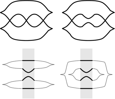
Figure 14. (i) Front diagram $\mathcal{D}$ and $\mathcal{D}_{\rho}$ for $\rho=\{b\}$; here $\rho$ is not a ruling. (ii) Normality condition for the ruling.

A ruling is oriented if every element of $\rho$ is a positive crossing. Let $\Gamma(\mathcal{D})$ and $O\Gamma(\mathcal{D})$ be the sets of rulings and oriented rulings, respectively.

For a ruling $\rho$ we define

$$j(\rho)=\#\rho-l\mbox{-cusp}(\mathcal{D})+1,$$

where $l\mbox{-cusp}(\mathcal{D})$ denotes the number of the left cusps of $\mathcal{D}$.

Let $tb(\mathcal{D})=w(\mathcal{D})-l\mbox{-cusp}(\mathcal{D})$ be the Thurston-Benneuqin invariant. Rutherford showed the following formula of the part of the Kauffman(Dubrovnik)/HOMFLY polynomials.

Theorem 11.5.

[Rut, Theorem 3.1, Theorem 4.3]

$$D_{L}(z;tb(\mathcal{D})+1)=\sum_{\rho\in\Gamma(\mathcal{D})}z^{j(\rho)},\quad P_{L}(z;tb(\mathcal{D})+1)=\sum_{\rho\in O\Gamma(\mathcal{D})}z^{j(\rho)}.$$ (11.2)

Thus, we have the following explanation of the coincidence and non-negativity.

Corollary 11.6.

If a link $L$ admits a front diagram $\mathcal{D}$ such that $\Gamma(\mathcal{D})=O\Gamma(\mathcal{D})$, then $D_{L}(z;tb(\mathcal{D})+1)=P_{L}(z;tb(\mathcal{D})+1)$ and it is a non-negative polynomial.

This gives a proof of Theorem 11.3 as follows.

Proof of Theorem 11.3.

As is discussed and proven in [Tan], one can view a positive diagram $D$ as a front diagram $\mathcal{D}$; we put each positive crossing so that it is in the form , and put each Seifert circle to form a front diagram having exactly two cusps so $l\mbox{-cusp}(\mathcal{D})=s(D)$.

Then the set of all crossings forms a (oriented) ruling. Thus $\mathcal{D}$ attains the maximum Thurston-Bennequin number. In particular,

$$\overline{tb}(K)=tb(\mathcal{D})=c(D)-s(D)=-\chi(D)=-\chi(K).$$

Moreover, since all the crossings of $\mathcal{D}$ are positive, $\Gamma(\mathcal{D})=O\Gamma(\mathcal{D})$, hence Corollary 11.6 gives the desired equality and non-negativity. ∎

A mild generalization shows that an almost positive link of type II (and a suitable loosely successively positive link) shares the same property.

Theorem 11.7.

If $K$ admits an almost positive diagram of type II, then

$$P_{K}(z;1-\chi(K))=D_{K}(z;1-\chi(K))\neq 0$$

and it is a non-negative polynomial.

Proof.

We view an almost positive diagram of type II as a front diagram $\mathcal{D}$ as shown in Figure 15, where the box represents a positive diagram part viewed as a front diagram as we mentioned earlier. (See [Tag] for a detailed discussion on how to achieve this, where the Lagrangian fillability of almost positive knots of type II is shown by similar methods and arguments.)

A ruling of $\mathcal{D}$ cannot contain the negative crossing of $\mathcal{D}$, so $\Gamma(\mathcal{D})=O\Gamma(\mathcal{D})$. On the other hand, since $D$ is of type II, the Seifert circles $s$ and $s^{\prime}$ connected by the negative crossing $c_{-}$ are also connected by a positive crossing. We take such a crossing $c$ so that there is no such crossing between $c$ and $c^{-}$. Let $\rho=C(\mathcal{D})\setminus\{c_{-},c\}$. Then $\rho$ is a ruling, so that $\Gamma(\mathcal{D})=O\Gamma(\mathcal{D})\neq\emptyset$, and

$$\overline{tb}(K)=tb(\mathcal{D})=(c(D)-2)-s(D)=-\chi(D)-2=-\chi(K).$$

∎

Corollary 11.8.

If $K$ is almost positive of type II,

$$\min\deg_{a}D_{K}(z,a)=\max\deg_{z}P_{K}(v,z)=1-\chi(K).$$

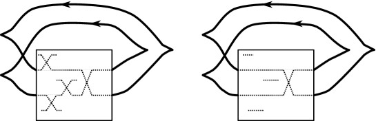
Figure 15. (i) Front diagram of almost positive diagram of type II; the box represents a front diagram consisting of positive crossings. (ii) Non-trivial ruling $\rho=C(\mathcal{D})\setminus\{c_{-},c\}$ and its resolution $\mathcal{D}_{\rho}$

By [St8, Theorem 1.4], there exists an almost positive knot that does not admit an almost positive diagram of type II. The example given there (the pretzel knot $P(3,3,3,3,-1)$) satisfies the equality (11.1). The second author also showed that these exists an almost positive knot that does not admit an almost positive diagram of type I.

We do not have an example of an almost positive knot that fails to have property (11.1), so the following question remains open.

Question 11.9.

Does equality (11.1) hold for almost positive links?

11.3. Good successively almost positive vs. loosely successively almost positive

Theorem 11.10.

There exists a loosely successively almost positive knot which is not a good successively almost positive knot. More precisely, the following three knots $15_{132907},15_{96757},15_{125012}$ given in Figure 16 are 15 crossing, genus 2 knots which are loosely successively almost positive but are not good successively almost positive.

$$\begin{array}[]{ccc}\includegraphics*[width=113.81102pt]{eps/17_730721.eps}&\includegraphics*[width=113.81102pt]{eps/15_132907.eps}&15_{132907}\\ \includegraphics*[width=113.81102pt]{eps/16_3.eps}&\includegraphics*[width=113.81102pt]{eps/15_96757.eps}&15_{96757}\\ \includegraphics*[width=113.81102pt]{eps/16_4.eps}&\includegraphics*[width=113.81102pt]{eps/15_125012.eps}&15_{125012}\\ \end{array}$$

Figure 16. Knots for Theorem 11.10. The first column gives a (loosely) successively 2-almost positive diagram (where the negative crossings appear on an underarc). The second column gives their diagrams as included in the table [HT].

The proof of Theorem 11.10 is based on the generator-twisting method of [St4], and we will frequently use the terminologies in Definition 2.4.

Definition 11.11.

An alternating diagram $D$ (or its knot) is a generator if each of its $\sim$-equivalence classes has no more than two crossings.

The terminology ‘generator’ is justified by the following theorem, which allows us to effectively enumerate all the diagrams of a given genus.

Theorem 11.12.

[Br, St1] For a given $g>0$, there exist only finitely many generators of genus $g$. All diagrams $D$ of genus $g$ are obtained from one of a generator by $\bar{t}^{\prime}_{2}$-twists, flypes, and crossing changes.

For later use we remark the following simple observations.

Lemma 11.13.

Let $D$ be a non-split diagram of Euler characteristic $\chi(D)$. Then

$$\sum_{\mbox{$S$:Seifert equivalence class}}(\#S-1)\leq 1-\chi(D).$$

Here $\#S$ denotes the number of crossings that belong to the the Seifert equivalence class $S$.

Proof.

Since $D$ is non-split, the number of Seifert equivalence classes is at least $s(D)-1$. Thus

$$\chi(D) =s(D)-c(D)=s(D)-\sum_{\mbox{$S$:Seifert equivalence class}}\#S$$

$$\leq 1-\sum_{\mbox{$S$:Seifert equivalence class}}(\#S-1).$$

∎

Lemma 11.14.

If a link $K$ admits a reduced successively $k$-almost positive positive diagram $D$, then

$$k\leq 1-\chi(D)\,.$$ (11.3)

Proof.

It is sufficient to consider the case $D$ is a non-split diagram. In a successively almost positive diagram $D$, any two successive negative crossings connect a separating Seifert circle from opposite sides. Decompose $D=D_{1}*\dots*D_{k}$ as a diagram Murasugi sum along these $k-1$ separating Seifert circles.

Let us write $D$ as $D_{1}\ast\cdots\ast D_{k}$, a diagram Murasugi sum of (good or loosely) almost positive diagrams $D_{1},\ldots,D_{k}$. Since $D$ is reduced, so are $D_{i}$. Thus $\chi(D_{i})\leq 0$, so we conclude $\chi(D)=\sum_{i=1}^{k}\chi(D_{i})-(k-1)\leq 1-k$. ∎

Proof of Theorem 11.10.

By Lemma 11.14, if any of the knots given in Figure 16 admits a reduced good successively $k$-almost positive diagram, then $k\leq 4$.

It is easy to see they are not positive; a positive genus 2 knot $K$ must satisfy $\max\deg Q(K)\geq c(K)-2$ for the $Q$-polynomial $Q(K)$ (see [St9]), and a direct computation shows that none of three knots in Figure 16 satisfies this inequality.

One can also confirm that $15_{132907},15_{96757},15_{125012}$ are not almost positive of type I (i.e., good successively $1$-almost positive), following the method in [St8], or the method similar to the following argument to rule out good successively $2$-almost positive (though in practice, there are several differences; see Remark 11.15 for details).

Here we give details on how to check $15_{132907},15_{96757},15_{125012}$ are not good successively 2-almost positive. A proof that they are not good successively $k$-almost positive for $k=3,4$ is similar.

We refer to the definition of the Alexander polynomial $\Delta$ in Section 2.7, and its properties which translate from corresponding properties of $\nabla$ under the conversion (2.9).

The knots $K\in\{15_{132907},15_{96757},15_{125012}\}$ in Figure 16 satisfy

$$\max\deg_{t}\Delta_{K}(t)=2,\mbox{ and }\max{\operator@font cf}\,\Delta_{K}\leq 9.$$

We show that they are not good successively 2-almost positive by enumerating all the good successively 2-almost positive diagrams of knots $K$ such that $g(K)=\max\deg\Delta=2$ and that $\max{\operator@font cf}\,\Delta\leq 9$. We checked that none of these diagrams represents any of the knots $15_{132907},15_{96757},15_{125012}$.

We determine the generating set $\mathcal{D}$ of successively 2-almost positive knot diagrams of genus $2$. That is, we determine a set $\mathcal{D}$ of diagrams having the following properties.

• Every good successively 2-almost positive knot $K$ of genus two admits a good successively 2-almost positive $D$ such that $D$ is obtained from one of the generators $D^{\prime}\in\mathcal{D}$ by applying $\bar{t}^{\prime}_{2}$-twists (10.14).

• $D^{\prime}$ is a successively 2-almost positive diagram.

Here and in the following, by $\bar{t}^{\prime}_{2}$-twists we always mean positive $\bar{t}^{\prime}_{2}$-twists.

Unlike properties like alternating, positive, or almost positive, it should be noted that the property that a diagram is successively 2-almost positive is not flype invariant. Hence flypes must be paid attention to. See Remark 11.15 for details on the treatment of flypes for good successively 1-almost positive.

The generating set $\mathcal{D}$ is determined in the following manner.

• Take a genus 2 generator diagram $D$.

• List all the diagrams obtained from $D$ by a flype. Then positivize the diagrams and switch two crossings to make $D$ successively $2$-almost positive.

• Reduce modulo type B flypes,

• Discard all diagrams with $\sim$-equivalent crossings of opposite sign.

• Apply (i)-(iv) for all genus 2 generator diagrams.

• Sort out duplicates.

Here the step (iii) means that we choose a (canonical, according to some deterministic criterion) minimal representative among a type B flype equivalence class of diagrams. (For type B flypes see, e.g., [St9, Fig. 5].) Since type B flypes commute with $\bar{t}^{\prime}_{2}$-twists, for our purpose, one can discard the diagrams related by type B flypes.

At the step (iv), among the successively $2$-almost positive diagrams obtained so far, we discard all diagrams with $\sim$-equivalent crossings of opposite sign. Even after $\bar{t}^{\prime}_{2}$-twists at the positive crossing(s), one can cancel $\sim$-equivalent positive and negative crossings, so that the diagram $D$ becomes positive or almost positive.

Having determined the generating set $\mathcal{D}$, we proceed to enumerate all the good successively $2$-almost positive knots having the properties $g(K)=\max\deg_{t}\Delta_{K}(t)=2$ and that $\max{\operator@font cf}\,\Delta\leq 9$.

To get a good successively 2-almost positive diagram, we need a twist at every positive crossing Seifert equivalent to a negative crossing. By Lemma 11.13, the number of such positive crossings is at most $1-\chi(D)=2g(D)=4$. Hence one can make a generator diagram $D\in\mathcal{D}$ into a good successively $2$-almost positive diagram by at most $4$ $\bar{t}^{\prime}_{2}$-twists. In particular, after at most $4$ $\bar{t}^{\prime}_{2}$-twists, we may always assume that $g(D)=\max\deg_{t}\Delta_{K}(t)=2$.

It follows from the properties $\max\deg_{t}\Delta_{K}(t)=g(D)$ and $\max{\operator@font cf}\,\Delta_{K}(D)>0$ for every successively 2-almost positive link diagram $D$ that $\max{\operator@font cf}\,\Delta_{K}(D)$ will always strictly increase under $\bar{t}^{\prime}_{2}$-twists. Since $\max{\operator@font cf}\,\Delta(D)\leq 9$, the number of $\bar{t}^{\prime}_{2}$-twists that can be applied is bounded by

$$(1-\chi(D))+\max{\operator@font cf}\,\Delta-1\,=\,4+9-1=12\,.$$ (11.4)

Thus by taking all the good successively positive diagrams obtained from a generator in the generating set $\mathcal{D}$ by at most $12$ $\bar{t}^{\prime}_{2}$-twists, we determine all the good successively almost positive knot diagrams of genus $2$ having the property $\max{\operator@font cf}\,\Delta\leq 9$.

By computing the Jones polynomials $V_{K}(t)$, we checked that these polynomials do not match with any of $15_{132907},15_{96757},15_{125012}$ except 9 diagrams (of 14 and 15 crossings). These remaining 9 diagrams locate to some 14 crossing knot, so we are done.

∎

With the necessary tools in place, the work can be carried out on a laptop within 45 minutes.

Remark 11.15.

The confirmation that $15_{132907},15_{96757},15_{125012}$ are not good successively $1$-almost positive is done by a similar method, but since the property that almost positive is invariant under flype, armed with the following observations we can reduce the size of the generating set $\mathcal{D}$ which makes computation faster.

Let $D^{\prime}$ be a diagram obtained from $D$ by flype, and assume that $\widetilde{D^{\prime}}$ is obtained from $D$ by $\bar{t}^{\prime}_{2}$-twists. Let $\widetilde{D}$ be a diagram obtained from $D$ by applying $\bar{t}^{\prime}_{2}$-twists at the corresponding crossings. Then $\widetilde{D^{\prime}}$ and $\widetilde{D}$ are related each other by mutation of diagrams (see, e.g., [St5]).

Thus, one can postpone taking into account the effect of the flypes until the last step, to modify the argument as follows.

• At the step (ii) of a construction of generating set, we just make a generator $D$ into almost positive diagram, by suitably changing the crossings (we do not apply flypes).

• At the final step, for a knot $K$ represented by a candidate diagram $D$, we check whether the Jones polynomial $V_{K}(t)$ of candidates are equal or not.

• Since the Jones polynomial is mutation invariant, if the Jones polynomials are different, any mutant of $D$ does not represent $15_{132907},15_{96757},15_{125012}$. When the Jones polynomial coincides (it seems to be rare), then we consider all the mutants of diagram $D$ and check all of them are not equal to $15_{132907},15_{96757},15_{125012}$ by other methods.

In the case of good (type I) almost positive diagrams, fortunately, every diagram can be distinguished from $15_{132907},15_{96757},15_{125012}$ by the Jones polynomial, so we do not need to consider mutants.

11.4. Good successively almost positive vs. almost positive

Theorem 11.16.

There exist knots which are good successively 2-almost positive but are not almost positive. More precisely, the knots $17_{*1614792},17_{*908691},17_{*549551}$ of Figure 17 are good successively 2-almost positive knots of genus 3 which are not almost positive. All three knots are checked to be 17 crossing knots.

$$\begin{array}[]{cc}\includegraphics*[width=128.0374pt]{eps/17_1614792.eps}&\includegraphics*[width=128.0374pt]{eps/17_908691.eps}\\ 17_{*1614792}&17_{*908691}\\[22.76219pt] \includegraphics*[width=128.0374pt]{eps/17_549551.eps}&\includegraphics*[width=128.0374pt]{eps/17_264313.eps}\\ \lx@intercol\hfil 17_{*549551}\hfil\lx@intercol\end{array}$$

Figure 17. Knots for Theorem 11.16. The first row diagrams and the left second row diagram are all good successively 2-almost positive minimal diagrams (where the negative crossings appear on an underarc). The third knot has some loosely successively 2-almost positive minimal diagrams also, e.g., the one shown in the second row right.

Proof.

A main stream of the proof is similar to Theorem 11.10 or [St8], which works for almost positive of type II (i.e., even if $\max\deg\Delta=g(D)-1=g(K)$). However, the three knots are fibered of genus 3, so $\max{\operator@font cf}\,\Delta_{K}=1$. This simplifies the argument as we will describe below.

First of all, checking that they are not positive can be done by Cromwell’s $c(K)\leq 4g(K)$ test [Cr] as in Section 11.1.

We show they are not almost positive. Let us take an almost positive generator diagrams of genus $3$ or $4$. These generators were compiled as in [St4, St9].

Case 1. $g(D)=4$ (i.e., $D$ is type II, or loosely successively 1-almost positive).

As in the proof of Theorem 11.10, $\bar{t}^{\prime}_{2}$-twists will always augment $\max{\operator@font cf}\,\Delta_{K}$ even if $\max\deg\Delta_{K}=3$, or will realize $\max\deg\Delta_{K}=4$. Thus $\max\deg\Delta_{K}=3$ and $\max{\operator@font cf}\,\Delta_{K}=1$ imply that we do not need to use $\bar{t}^{\prime}_{2}$-twists. Thus only almost positive generator diagrams of genus 4 need to be tested.

To further reduce work, we use that all three knots $K$ have signature $\sigma(K)=4$, which means that positivized (genus 4) generators $D$ must have $\sigma(D)\leq 6$. It (drastically) reduces the number of generators to consider.

Again one can pre-select diagrams by checking the coincidences of the Jones polynomial $V_{K}(t)$. It turns out that the Jones polynomial already distinguishes all these diagrams from any of the three knots. Since $\bar{t}^{\prime}_{2}$-twists are not applied, unlike Remark 11.15 no mutations need to be taken care of.

The test can be performed in a few minutes.

Case 2. $g(D)=3$ (i.e., $D$ is good, or type I).

Here twisting must be tested, and it was performed similarly to the proof of Theorem 11.10, but again keeping eye on the signature (as in Case 11.4) and additionally using tests of the maximal value of the coefficients of $\nabla$ of the three knots (which is attained by $17_{*549551}$ for both $z$-degree $2$ and $4$).

As we argued above, a $\bar{t}^{\prime}_{2}$-twist must be performed on each crossing Seifert equivalent to the negative one (otherwise $\max\deg\Delta<3$) but at no other crossing (otherwise if $\max\deg\Delta=3$, then $\max{\operator@font cf}\,\Delta>1$). By Lemma 11.13, in particular at most $6$ twists need to be applied. But one can easily see that $6$ twists are needed only for (the series of) $7_{1}$ and $5$ twists only for some 8-crossing generators.

There is a number of redundancies still left, but avoiding further (very technical) simplifications, the test was manageable in about 50 minutes on a laptop. ∎

11.5. (Good) Successively almost positive vs. strongly quasipositive

Strongly quasipositive knots are not necessarily successively almost positive; for a given link $L$, there exists a strongly quasipositive link $L^{\prime}$ such that $\nabla_{L}(z)=\nabla_{L^{\prime}}(z)$ [Rud6, 88 Corollary]. See [Si, Section 5] for details and concrete examples. Thus the Conway polynomial of strongly quasipositive link may not be non-negative.

11.6. Enumeration of positive knots

A similar method to the one used for Theorem 11.10 or Theorem 11.16 can also overcome the problems of [AT] which asks whether some almost positive knots are non-positive or not, although we need various additional simplifications to make computation faster and reasonable. In particular, a similar method allows us to complete the list of low-crossing positive (prime) knots.

For positive diagrams, since the value $\max{\operator@font cf}\,\Delta$ is generally higher, the bound on the number of $\bar{t}^{\prime}_{2}$-twists in (11.4) is large, so the number of candidate diagrams will be much larger.

To reduce the computation, we exploit a useful fact that a positive diagram $D$ is A-adequate ($+$-adequate),

By [St7, Proposition 3.4] (which is the reinterpretation of Thistlethwaite’s work [Th] on A-adequacy ($+$-adequacy)), for a positive diagram $D$ of $K$

$$\max\deg_{z}F_{K}(a,z)\geq c(D)-1+\chi(D)$$

holds. Since one $\bar{t}^{\prime}_{2}$-twist increases $c(D)$ by two, if $K$ is obtained from a generator $D_{0}$ by $\bar{t}^{\prime}_{2}$-twists $k$ times,

$$1-\chi(D_{0})+\max\deg_{z}F_{K}(a,z)-c(D_{0})\geq 2k$$

holds. This bound is often far better than the bound $k\leq\max{\operator@font cf}\,\Delta_{K}-1$, which is the analogue of (11.4) for a positive diagram. (In (11.4), the first term $1-\chi(D)$ on the left hand side has appeared to make the diagram good. Thus for a positive diagram we do not need this term.)

It took a few hours on a desktop for up to 13 crossings and about 3 days for 14-15 crossings, although it will very likely not be able to (easily) completely settle the list for 16 crossings. The result (232 prime non-alternating knots up to 13, and 3355 knots of 14-15 crossings) is available on [St13]. Some more detailed account on the computation will take up extra space and may be given elsewhere. Here we just state the following answer to [AT, Question 6.9].

Theorem 11.17.

Up to $12$ crossings, there are $13$ almost positive, but not positive prime knots:

$$\begin{array}[]{c}10_{145},\ 12_{1436},\ 12_{1437},\ 12_{1564},\ 12_{1617},\ 12_{1620},12_{1654},\\ 12_{1690},\ 12_{1692},\ 12_{1720},\ 12_{1816},\ 12_{1930},\ 12_{1948}\,.\end{array}$$

Proof.

These knots are shown to be almost positive in [AT]. That they are non-positive can be checked by the generator-twisting method as we discussed.

Corollary 8.3 and the methods of Appendix B give alternative proofs of the non-almost positivity of the remaining knots, except for $12_{1811}$ and $12_{2037}$. The first one has zero signature so it cannot be almost positive (indeed, by Theorem 9.1 it cannot be w.s.a.p.).

The second one has $g_{3}(K)\neq g_{4}(K)$ so it is not Bennequin sharp. Since an almost positive knot is Bennequin sharp, $K$ cannot be almost positive.

∎

It must be noted also that, while semiadequacy input is not useful for non-positive diagrams in general, there are tools available to use polynomial degrees to reduce twisting in non-positive diagrams as well. Such “regularization” tests were extensively elaborated on in [St11]. We avoided these technicalities for Theorem 11.10, since the number of diagrams left to check (about 34,000) was fairly manageable anyway.

11.7. Weakly successively almost positive vs. weakly positive

By means of Example 4.2, take many 2-almost positive knots, like the figure-8-knot. Many of the properties of weakly successively almost positive knots we proved (like positivity of $\nabla$) are not satisfied.

12. Questions and problems

Throughout the paper we raised various questions or conjectures. In this section we gather a set of problems arising from various discussions in the paper.

Though to save the space we mainly concentrate on weakly successively almost positive links, a similar question is always meaningful if we restrict it to some more specific class like (good/loosely) successively almost positive links.

The most important open problem for weakly successively almost positive links is their strong quasipositivity.

Question 12.1.

• Is every weakly successively almost positive link strongly quasipositive ?

• Is every weakly successively almost positive link Bennequin-sharp ?

• Is every weakly successively almost positive link quasipositive ?

As outlined, we will address these questions, to some extent, in [IS].

We have seen that various classes of positivity notions are indeed different, by showing the canonical inclusion is strict. Nevertheless, there are still several inclusions whose strictness is not confirmed yet. In light of Theorem 11.10 or Theorem 11.16, it is natural to expect the affirmative answer to the following.

Question 12.2.

Is there a weakly successively almost positive link which is not successively almost positive ?

See Remark 11.2 for the corresponding problems where the number $k$ of negative crossings is fixed. In a similar direction, it is also natural to ask the following.

Question 12.3.

For every $k>0$, is there a weakly successively $k$-almost positive link which is not weakly successively $k^{\prime}$-almost positive of all $k^{\prime}<k$ ?

The same question applies for successively almost positive. It should be noted that the method in Theorem 11.10 or Theorem 11.16, in principle, works for higher fixed $k$. But it is already difficult to practice for $k=3$, and certainly leaves unclear at present how to simultaneously construct examples for arbitrary $k$ (or, in fact, infinitely many $k$ for that matter).

We have seen various properties of invariants of a w.s.a.p. link that are generalizations of properties of a positive link (under the additional assumption that it is Bennequin-sharp, if needed).

Nevertheless, there are several properties which remain open.

Question 12.4.

Let $L$ be a weakly successively almost positive link.

• If $L$ is fibered, is the unique non-zero coefficient $c_{k,1-\chi(L)}$ always $c_{1-\chi(L),1-\chi(L)}=1$ ? (Conjecture 7.3)

• Does the maximum $z$-degree term of the HOMFLY polynomial of w.s.a.p. link have the gap-free property ? (see Remark 8.2)

• Does the equality (11.1) hold for almost positive links of type I ? More generally, does equality (11.1) hold for (good) successively almost positive links?

In Theorem 10.3 we showed the finiteness of (weakly) successively almost positive knots in an algebraic concordance class, for weakly successively $k$-almost positive knots for fixed $k$. It is natural to ask whether fixing $k$ is necessary or not.

Question 12.5.

Does every algebraic (or, topological, smooth) concordance class contain at most finitely many weakly successively almost positive knots?

In a related direction, it is of independent interest to explore an optimal signature estimate from (w.s.a.p.) diagram.

Question 12.6.

Let $D$ be a reduced diagram of a link $L$. Find optimal coefficients $C_{1},C_{2}$ so that

$$\sigma(L)\geq C_{1}(1-\chi(L))-C_{2}c_{-}(D)$$

Similarly, for a reduced w.s.a.p. diagram $D$ of $L$, find optimal coefficients $C^{\prime}_{1},C^{\prime}_{2}$ so that

$$\sigma(L)\geq C^{\prime}_{1}(1-\chi(L))-C^{\prime}_{2}c_{-}(D)$$

In [Oz] Ozawa showed the visibility of primeness for positive diagrams: a link represented by a positive diagram $D$ is non-prime if and only if the diagram $D$ is non-prime. As a consequence, if $K_{1}\#K_{2}$ is positive, then both $K_{1}$ and $K_{2}$ are positive.

A straightforward generalization for (good) successively almost positive diagrams does not hold.

Example 12.7.

The knot diagram on Figure 18 is a good successively 2-almost positive diagram of $3_{1}\#10_{145}$ which is not prime ($3_{1}$ is positive and $10_{145}$ is almost positive).

$$\begin{array}[]{c}\includegraphics*[width=128.0374pt]{eps/17_684.eps}\\ 3_{1}\#10_{145}\end{array}$$

Figure 18. A prime good successively $2$-almost positive diagram of a composite knot.

Obviously one can construct such examples for good successively $1$-almost positive as well.

The question and observation suggest that when we discuss (good) successively $k$-almost positive diagrams, it is better and more natural to take the minimum $k$.

Definition 12.8.

We say that a (weakly) successively almost $k$-positive diagram $D$ of a link $L$ is tight if $k$ (the number of negative crossings) is minimum among all the (weakly) successively almost positive diagram of $L$.

Let us define

$$p_{good}(K)=\min\{k\>|\>K\mbox{ is good successively }k\mbox{-almost positive}\}$$

if $K$ is good successively almost positive, and $p(K)=-\infty$ otherwise. Similarly, we define

$$p_{succ}(K)=\min\{k\>|\>K\mbox{ is (weakly) successively }k\mbox{-almost positive}\}$$

if $K$ is (weakly) successively almost positive, and set $p_{succ}(K)=-\infty$ otherwise.

The following way of extending Ozawa’s result, modified to evade the previous counterexample, could still be true.

Question 12.9.

Is a knot $K$ prime if $K$ is represented by a prime tight w.s.a.p. diagram $D$ ?

Although Question 12.9 seems not previously encountered even for $k=1$, at least thus far it appears worth asking: If a prime (good) almost positive diagram depicts a composite knot, is the knot positive (i.e., the connected sum of positive factors)?

The technicality of determining $p_{succ}(K)$ or $p_{good}(K)$ also raises the question about a property that can more naturally distinguish (almost) positive links from (good) successively almost positive ones.

Investigating these quantities will be of independent interest. For instance, Lemma 11.14 implies that $p_{good}(K)\leq 1-\chi(K)$. Finding other upper or lower bounds would be useful to attack Question 12.3. Note also that the condition (10.13) is of similar nature, and its weakening, together with Lemma 11.14, is a potential strategy towards Question 12.5.

We have seen the evidence for the remarks at the start of Section 11. But they also underscore the difficulty of Question 12.3 as to understanding the filtration of successively almost positive links with respect to $p_{succ}(K)$.

In this regard, we pose one more natural problem related to Question 12.9:

Question 12.10.

Is $K_{1}\#K_{2}$ w.s.a.p. (s.a.p.) if and only if both $K_{1}$ and $K_{2}$ are so? Is $p_{succ}(K_{1}\#K_{2})=p_{succ}(K_{1})+p_{succ}(K_{2})$ (similarly for $p_{good}$)?

Appendix A. Fibered link enhancement for Scharlemann-Thompson’s theorem

In this appendix we prove Theorem 6.2. Our proof is a mild extension of Scharlemann-Thompson’s proof using sutured manifold theory.

A.1. Sutured manifold

Definition A.1.

A sutured manifold $(M,\gamma)$ is a pair of an irreducible oriented compact 3-manifold $M$ and a subset $\gamma\subset\partial M$ consisting of pairwise disjoint annuli such that each annulus contains an oriented core circle.

The suture $s(\gamma)$ is the union of the oriented core circles of the annuli $\gamma$. We orient each component of $R(\gamma):=\partial M\setminus\gamma$ so that the orientation is coherent with the orientation of the sutures (i.e., the orientation of $\partial R$ coincides with that of the sutures). We denote by $R_{+}(\gamma)$ (resp. $R_{-}(\gamma)$) the union of the components of $R(\gamma)$ such that the orientation agrees (resp. disagrees) with the orientation as a subsurface of $\partial M$.

Definition A.2.

A sutured manifold $(M,\gamma)$ is taut if $R(\gamma)$ is a Thurston norm-minimizing in $H_{2}(M,\gamma)$.

Example A.3 (Trivial sutured manifold, product sutured manifold).

A sutured manifold $(M,\gamma)$ is a product sutured manifold if it is homeomorphic to $(S\times[0,1],\partial S\times[0,1])$ for some compact oriented surface $S$. When $S=D^{2}$, we say that $(M,\gamma)$ is the trivial sutured manifold.

Example A.4 (Complementary sutured manifold).

Let $R$ be a Seifert surface of (non-split) link $L$ in $M$. The complementary sutured manifold $(M_{R},\gamma_{R})$ of $R$ is a sutured manifold $(M\setminus(-1,1)\times R,\partial R\times[-1,1])$.

For a sutured manifold $(M,\gamma)$ and a properly embedded surface $S$ that transversely intersects with the sutures $s(\gamma)$, let $M^{\prime}$ be the 3-manifold obtained from $M$ by cutting along $S$. Then by connecting sutures naturally, we get a sutured manifold $(M^{\prime},\gamma^{\prime})$. We refer to such a situation as $S$ defines a sutured manifold decomposition $(M,\gamma)\stackrel{{\scriptstyle S}}{{\rightsquigarrow}}(M^{\prime},\gamma^{\prime})$.

For example, the complementary sutured manifold $(M_{R},\gamma_{R})$ of a Seifert surface $R$ can be seen as a sutured manifold decomposition $(M,\emptyset)\stackrel{{\scriptstyle R}}{{\rightsquigarrow}}(M^{\prime},\gamma^{\prime})$ defined by $R$.

A key feature of a sutured manifold decomposition is the following.

Lemma A.5.

[Ga2, Lemma 3.5] Let $(M,\gamma)\stackrel{{\scriptstyle S}}{{\rightsquigarrow}}(M^{\prime},\gamma^{\prime})$ be a sutured manifold decomposition. If $(M^{\prime},\gamma^{\prime})$ is taut, then $(M,\gamma)$ is taut.

Definition A.6.

Let $(M,\gamma)$ be a sutured manifold. A product annulus is a properly embedded annulus $A$ in $M$ such that $\partial A\subset R(\gamma)$ and $\partial A\cap R_{\pm}(\gamma)\neq\emptyset$. A product disk is a properly embedded disk $D$ in $M$ such that $\gamma\cap D$ is two essential arcs.

A product decomposition is a sutured manifold decomposition $(M,\gamma)\stackrel{{\scriptstyle\Delta}}{{\rightsquigarrow}}(M^{\prime},\gamma^{\prime})$ defined by a product disk $\Delta$.

The following lemma explains a relation between a product disk/annulus and product sutured manifolds.

Lemma A.7.

[Ga4, Lemma 2.2, Lemma 2.5] Let $(M,\gamma)\stackrel{{\scriptstyle S}}{{\rightsquigarrow}}(M^{\prime},\gamma^{\prime})$ be a sutured manifold decomposition defined by a product disk or a product annulus $S$. Then $(M,\gamma)$ is a product sutured manifold if and only if $(M^{\prime},\gamma^{\prime})$ is a product sutured manifold.

A.2. Norm-reducing slopes

Let $M$ be an irreducible 3-manifold whose boundary is a non-empty union of tori, and let $P$ be a component of $\partial M$. For a slope (unoriented simple closed curve) $s$ of $P$, we denote by $M(s)$ the Dehn filling on $s$.

Let $S$ be a properly embedded surface such that $P\cap S=\emptyset$. In this section we review a slope $\alpha$ where $S$ (can) fail to be norm-minimizing in $M(\alpha)$. See [BT] for more general results on how the Thurston norm behaves under Dehn fillings.

Definition A.8.

An $I$-cobordism between surfaces $S_{0}$ and $S_{1}$ is a 3-manifold $V$ whose boundary is $S_{0}\cup S_{1}$ such that the induced maps $(i_{j})_{*}:H_{1}(S_{j})\rightarrow H_{1}(V)$, $(j=0,1)$ are both injective.

Let $P$ be a torus boundary component of $\partial M$ and $S$ be a properly embedded surface in $M$ which is disjoint from $S$. We say that $M$ is $S_{P}$-atoroidal if, whenever cutting $M$ along a torus $T$ in $M\setminus S$ (and taking a suitable component) gives rise to an $I$-cobordism between $P$ and $T$, then $T$ is parallel to $P$.

To understand norm-reducing slopes, the following existence theorem of sutured manifold hierarchy plays a fundamental role.

Theorem A.9.

[Ga5, Step 1 of the proof of Theorem 1.7] Let $R$ be a norm-minimizing surface which is disjoint from $P$, and let $(M_{R},\gamma_{R})$ be the complementary sutured manifold of $R$. Then there exists a taut sutured manifold hierarchy

$$(M_{R},\gamma_{R})\stackrel{{\scriptstyle S_{1}}}{{\rightsquigarrow}}(M_{1},\gamma_{1})\stackrel{{\scriptstyle S_{2}}}{{\rightsquigarrow}}\cdots\stackrel{{\scriptstyle S_{n}}}{{\rightsquigarrow}}(M_{n},\gamma_{n}),$$ (A.1)

such that

• Each separating component of $S_{i}$ is a product disk.

• Each non-separating component of $S_{i}$ is either a product disk, or a norm-minimizing surface realizing some non-trivial $y\in H_{2}(H,\partial H)$ which is disjoint from $P$. Here $H$ denotes the connected component of $M_{i-1}$ that contains $P$.

• $(M_{n},\gamma_{n})$ is a union of trivial sutured manifolds and an $I$-cobordism between a torus $T$ and $P$ with non-empty sutures on $T$.

To simplify the notation, in the following arguments we always assume that the surfaces $S_{i}$ in (A.1) are connected. We will also neglect trivial sutured manifolds components to simply regard $(M_{n},\gamma_{n})$ as an $I$-cobordism between a torus $T$ and $P$.

Theorem A.10.

[Ga5, Theorem 1.8] Assume that $M$ is irreducible and $S_{P}$-atoroidal. Then the surface $S$ remains to be norm-minimizing in $M(s)$, for all but one slope $s$.

To give a precise description of the (possible) exceptional slope $s$, we review the proof.

Proof.

Take a sutured manifold hierarchy (A.1) given in Theorem A.9. The assumption that $M$ is $S_{P}$-atoroidal says that $M_{n}\cong P\times[0,1]$. Let $s$ be a slope on $P$ defined by the suture on $T=P\times\{1\}$. We call the slope $s$ the suture slope (with respect to the sutured manifold hierarchy (A.1)).

Let us consider the Dehn filling of $M(s^{\prime})$ of a slope $s^{\prime}$ on $P$, for $s\neq s^{\prime}$. Then by attaching solid tori along $P$ at each stage, the sutured manifold hierarchy (A.1) yields the sutured manifold hierarchy

$$(M_{S}(s^{\prime}),\gamma_{S})\stackrel{{\scriptstyle S_{1}}}{{\rightsquigarrow}}(M_{1}(s^{\prime}),\gamma_{1})\stackrel{{\scriptstyle S_{2}}}{{\rightsquigarrow}}\cdots\stackrel{{\scriptstyle S_{n}}}{{\rightsquigarrow}}(M_{n}(s^{\prime}),\gamma^{\prime}_{n})$$

Since we have assumed that $s^{\prime}$ is not equal to the suture slope $s$, the slope $s^{\prime}$ does not bound a disk in the solid torus in $M_{n}(s^{\prime})\cong D^{2}\times S^{1}$. This means that we can further apply the sutured manifold decomposition

$$(M_{n}(s^{\prime}),\gamma_{n})\stackrel{{\scriptstyle\Delta}}{{\rightsquigarrow}}(M_{n+1}(s^{\prime}),\gamma_{n+1})$$

along the meridional disk $\Delta$ to eventually get the trivial sutured manifold $(M_{n+1}(s^{\prime}),\gamma_{n+1})$. By Lemma A.5 this implies that the sutured manifold $(M_{S}(s^{\prime}),\emptyset)$ is taut, hence $S\subset M(s^{\prime})$ is norm-minimizing. ∎

Remark A.11.

By some additional arguments, as is stated and proven in [Ga5, Corollary 2.4], the conclusion of Theorem A.10 remains to be true without assuming the $S_{P}$-atoroidality assumption.

A.3. Scharlemann-Thompson theorem and its enhancement

We proceed to prove the fibered link enhancement of Scharlemann-Thompson’s theorem.

For the skein triple $(L_{+},L_{0},L_{-})$ formed at the crossing $c$, let $D$ be the crossing disk at $c$, and let $K=\partial D$. Let $R=R_{+}$ be a Seifert surface of $L=L_{+}$ contained in $S^{3}\setminus K$ that attains the maximum Euler characteristic among such Seifert surfaces (so it can happen that $\chi(L_{+})\neq\chi(R)$). We can put $R$ so that its intersection $R\cap D$ is a single arc $\alpha$. By splitting $R$ along $\alpha$, we get a Seifert surface $R_{0}$ of $L_{0}$. By $(-1)$ surgery on $K$ we get a link $L_{-}$, and $R$ gives rise to a Seifert surface $R_{-}$ of $L_{-}$ (see Figure 19).

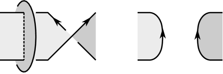
Figure 19. Crossing disk $D$ (left) and Seifert surface $R_{0}$ of $L_{0}$ (right).

Using these terminologies, the Scharlemann-Thompson theorem is stated in the following manner which contains additional information.

Theorem A.12.

(Scharlemann-Thompson theorem, slightly more precise version) At least two of $(R_{+},R_{-},R_{0})$ are norm-minimizing (i.e., attain the maximum Euler characteristic as a Seifert surface in $S^{3}$).

To explain which can be the largest among $\{\chi(R_{+}),\chi(R_{-}),\chi(R_{0})-1\}$ (i.e., which can fail to be norm-minimizing) we review the proof.

Proof.

Let $M=S^{3}\setminus N(L\cup K)$ be the complement of the link $L\cup K$, and let $P$ be the torus boundary component of $M$ which comes from $K$. By looking at the split factor of $L$ that contains the skein crossing, in the following we always assume that $L$ is non-split and that $M$ is irreducible. Let $M_{0},M_{-},M_{+}(=M)$ be the $0,-1,\infty$ surgery on $K$.

When $M$ is not $R_{P}$-atoroidal, Scharlemann-Thompson showed that [ST, Subclaim (a), (b)]

$$M_{\pm}\mbox{ are irreducible and }R_{\pm}\mbox{ are norm-minimizing}.$$ (A.2)

Thus in the following we assume that $M$ is $R_{P}$-atoroidal.

In this case, the Seifert surface $R_{0}$ of $L_{0}$ is related to the surface $R\subset M_{0}$ in the following manner.

Claim 1.

[ST, Claim 2] Let $(M,\gamma)$ be the complementary sutured manifold for $R\subset M_{0}$, and let $(M_{R_{0}},\gamma_{R_{0}})$ be the complementary sutured manifold for $S_{0}\subset S^{3}$. Then there is a product disk decomposition

$$(M,\gamma)\stackrel{{\scriptstyle\Delta}}{{\rightsquigarrow}}(M_{R_{0}},\gamma_{R_{0}})$$

Then the assertion follows from Theorem A.10; as we have seen, $R\subset S^{3}\setminus(L\cup\partial D)$ remains norm-minimizing for every Dehn filling on a slope $\alpha$ of $\partial D^{2}$ with at most one exception. The possible exception $\alpha$ is equal to the suture slope $s$ (with respect to some sutured manifold hierarchy (A.1)). ∎

The fibered link enhancement can be proven in a similar manner, by adding some additional arguments on the sutured manifold hierarchy.

Proof of Theorem 6.2.

(i) Assume that $\chi(L_{+})=\chi(L_{0})+1<\chi(L_{-})$ and that $L_{0}$ is fibered, hence $R_{0}$ is a fiber surface for $L_{0}$.

Then $L_{0}$ is not split so $M_{0}$ is irreducible. If $M$ is not $R_{P}$-atoroidal, then by (A.2) $R_{\pm}\subset M_{\pm}$ are norm-minimizing. This contradicts the assumption $\chi(L_{+})<\chi(L_{-})$, so $M$ is $R_{P}$-atoroidal.

Let $(M_{R},\gamma_{R})$ be the complementary sutured manifold of $R\subset S^{3}$. Since $\chi(L_{+})<\chi(L_{-})$, $R_{-}$ is not norm-minimizing in $M_{-}$. Thus by Theorem A.9 there is a sutured manifold hierarchy

$$(M_{R},\gamma_{R})\stackrel{{\scriptstyle S_{1}}}{{\rightsquigarrow}}(M_{1},\gamma_{1})\stackrel{{\scriptstyle S_{2}}}{{\rightsquigarrow}}\cdots\stackrel{{\scriptstyle S_{n}}}{{\rightsquigarrow}}(M_{n},\gamma_{n}).$$ (A.3)

such that its suture slope is $-1$.

On the other hand, since $R_{0}$ is a fiber surface of $L_{0}$, by Lemma A.7, the complementary sutured manifold $(M_{R_{0}},\gamma_{R_{0}})$ of $R_{0}\subset S^{3}$ is a product sutured manifold. By Claim 1 and Lemma A.7, this implies that the complementary sutured manifold $(M,\gamma)$ of $R\subset M_{0}$ is a product sutured manifold.

Let us take the taut sutured manifold hierarchy obtained from (A.3) by $0$-surgery on each torus $P$:

$$(M,\gamma)=(M_{R}(0),\gamma_{R})\stackrel{{\scriptstyle S_{1}}}{{\rightsquigarrow}}(M_{1}(0),\gamma_{1})\stackrel{{\scriptstyle S_{2}}}{{\rightsquigarrow}}\cdots\stackrel{{\scriptstyle S_{n}}}{{\rightsquigarrow}}(M_{n}(0),\gamma_{n}).$$

By Theorem A.9 (ii), if $S_{1}$ is not a product disk, $S_{1}$ is non-separating and $-S_{1}$ also defines a taut sutured manifold decomposition. Therefore by [Ga4, Corollary 2.7], we have that $S_{1}$ is a product annulus. Then $S_{1}$ is either a product disk or a product annulus, so by Lemma A.7 $(M_{1}(0),\gamma_{1})$ is a product sutured manifold. Repeating the same argument, we conclude that $S_{i}$ is either a product disk or a product annulus, and $(M_{i}(0),\gamma_{i})$ is a product sutured manifold for all $i$.

Therefore the suture of $\gamma_{n}$ of $M_{n}=P\times[0,1]$ consists of two curves of slope $-1$. This shows that $(M_{n}(\infty),\gamma_{n})$ is also a product sutured manifold. Let us take the taut sutured manifold hierarchy obtained from (A.3) by $\infty$-surgery on each torus $P$

$$(M_{R}(\infty),\gamma_{R})\stackrel{{\scriptstyle S_{1}}}{{\rightsquigarrow}}(M_{1}(\infty),\gamma_{1})\stackrel{{\scriptstyle S_{2}}}{{\rightsquigarrow}}\cdots\stackrel{{\scriptstyle S_{n}}}{{\rightsquigarrow}}(M_{n}(\infty),\gamma_{n}).$$

Since we have seen that each $S_{i}$ is a product disk or a product annulus, $(M_{R}(\infty),\gamma_{R})$, the complementary sutured manifold of $R\subset S^{3}$, is a product sutured manifold by Lemma A.7. Therefore $R$ is a fiber surface of $L=L_{+}$.

(ii) We assume that $\chi(L_{+})=\chi(L_{0})+1<\chi(L_{-})$ and that $L_{-}$ is fibered with fiber surface $R_{-}$. If $M$ is not $R_{P}$-atoroidal, then $L_{-}$ is a satellite link with winding number zero. However, this contradicts the assumption that $L_{-}$ is fibered because winding number zero satellite implies that the commutator subgroup of $\pi_{1}(S^{3}\setminus L_{-})$ contains the fundamental group of the companion torus $\pi_{1}(T)\cong\mathbb{Z}\oplus\mathbb{Z}$, so it cannot be the free group.

Thus in this case $M$ is $R_{P}$-atoroidal. The rest of the argument is the same; $R_{0}$ being not norm-minimizing implies that we can find a sutured manifold hierarchy of the complementary sutured manifold $(M_{R},\gamma_{R})$ so that the suture slope is $0$. That $R_{-}$ is a fiber surface implies that each $S_{i}$ in the sutured manifold hierarchy is a product disk or a product annulus, and the suture of $(M_{n},\gamma_{n})$ consists of two curves of slope $0$. Hence $(M_{n}(\infty),\gamma_{n})$ is also a product sutured manifold. By Lemma A.7 this implies that $(M_{R}(\infty),\gamma_{R})$ is a product sutured manifold, hence $R$ is a fiber surface of $L=L_{+}$. ∎

Appendix B. Knot table

B.1. The Rolfsen knots (prime knots up to 10 crossings)

We discuss here briefly which of the knots in Rolfsen’s knot table are s.a.p. or w.s.a.p. The answer is: only the obvious ones.

Theorem B.1.

Up 10 crossings, a prime knot $K$ is weakly successively almost positive if and only if it is either positive or almost positive.

Proof.

By Corollary 7.2 it is sufficient to treat non-alternating knots.

For non-alternating knots which are not almost positive (or positive), we find that Theorem 6.4 (ii) and Theorem 7.1 (i-a) shows that they are not w.s.a.p., with the following exceptions.

• The knot $10_{140}$. This knot is not w.s.a.p. since its HOMFLY polynomial does not satisfy Theorem 7.1 (i-b).

• The knot $10_{132}$. This knot has the same HOMFLY polynomial as the positive knot $5_{1}$. This knot is not w.s.a.p. because its signature is $0$. (By Theorem 9.1, the signature of w.s.a.p. knot is always positive.)

∎

B.2. Prime 11 and 12 crossing knots

As for knots up to 12 crossings, we have a result as follows.

Theorem B.2.

Up to 12 crossings, a prime knot $K$ is weakly successively almost positive if and only if it is either positive or almost positive, possibly except $12_{1408},\ 12_{1487},\ 12_{1837},\ 12_{2037}$.

Proof.

As in the Rolfsen’s knot table case, Theorem 6.4 (ii) and Theorem 7.1 (i-a) also deals with the non-alternating prime 11 crossing knots whose table diagram in [HT] is not positive or almost positive. (Only for $11_{379}$ we need Theorem 7.1 (i-b).)

Applying the same test on non-alternating 12 crossing knots, we find that the theorems also settle most, except 12.

• Four of them, $12_{1581}$, $12_{1609}$, $12_{2038}$ and $12_{2118}$, fall to Theorem 7.1 (i-d).

• Another four, $12_{1409}$, $12_{1488}$, $12_{1811}$, $12_{1870}$, fall to Theorem 9.1.

• The remaining 4 knots $12_{1408},\ 12_{1487},\ 12_{1837},\ 12_{2037}$ are the simplest prime knots for which we cannot decide yet on the w.s.a.p. (and s.a.p.) property.

∎

As a final note, we do not wish to imply that the decision for composite knots easily follows from that on their factors. Some connected sums like those in Examples 9.15 and 9.16 clearly appeal to this circumstance. There is the corresponding Question 12.10, which is unresolved.

References

- [AT] T. Abe and K. Tagami, Characterization of positive links and the -invariant for links, Canad. J. Math. 69(6) (2017), 1201–1218.
- [AH] K. Appel and W. Haken, Every planar map is four colorable, Contemporary Mathematics, 98. American Mathematical Society, Providence, RI, 1989. xvi+741 pp.
- [AK] N. Askitas and E. Kalfagianni, On knot adjacency, Topol. Appl. 126(1-2) (2002), 63–81.
- [BDL] S. Baader, P. Dehornoy, and L. Liechti, Signature and concordance of positive knots. Bull. Lond. Math. Soc. 50(1) (2018), 166–173.
- [BT] K. Baker and S. Taylor, Dehn filling and the Thurston norm. J. Differential Geom. 112(3) (2019), 391–409.
- [BW] A. Beliakova, and S. Wehrli, Categorification of the colored Jones polynomial and Rasmussen invariant of links, Canad. J. Math. 60(6) (2008), 1240–1266.
- [Be] D. Bennequin, Entrelacements et équations de Pfaff. Third Schnepfenried geometry conference, Vol. 1 (Schnepfenried, 1982), 87–161, Astérisque, 107-108, Soc. Math. France, Paris, 1983.
- [Br] M. Brittenham, Bounding canonical genus bounds volume, preprint (1998), available at https://www.math.unl.edu/~mbrittenham2/papers/.
- [Bu] J. v. Buskirk, Positive links have positive Conway polynomial, Springer Lecture Notes in Math. 1144 (1983), 146–159.
- [Ca] A. Cavallo, The concordance invariant tau in link grid homology, Algebr. Geom. Topol. 18(4) (2018), 1917–1951.
- [CC] A. Cavallo and C. Collari, Slice-torus concordance invariants and Whitehead doubles of links, Canad. J. Math. 72(6) (2020), 1423–1462.
- [Co] A. Conway The Levine-Tristram signature: a survey. 2019–20 MATRIX annals, 31 –56, MATRIX Book Ser., 4, Springer, Cham, 2021.
- [Cr] P. Cromwell, Homogeneous links, J. London Math. Soc. (2) 39(3) (1989), 535–552.
- [Et] J. Etnyre, Legendrian and transversal knots, Handbook of knot theory, 105–185, Elsevier B. V., Amsterdam, 2005.
- [FLL] P. Feller, L. Lewark and A. Lobb, Almost positive links are strongly quasipositive, Math. Ann., to appear.
- [Ga] D. Gabai, The Murasugi sum is a natural geometric operation. Low-dimensional topology (San Francisco, Calif., 1981), 131–143, Contemp. Math., 20, Amer. Math. Soc., Providence, RI, 1983.
- [Ga2] D. Gabai, Foliations and the topology of 3-manifolds. J. Differential Geom. 18(3) (1983), 445–503.
- [Ga3] D. Gabai, The Murasugi sum is a natural geometric operation. II. Combinatorial methods in topology and algebraic geometry (Rochester, N.Y., 1982), 93–100, Contemp. Math.44, Amer. Math. Soc., Providence, RI, 1985.
- [Ga4] D. Gabai, Detecting fibred links in . Comment. Math. Helv. 61(4) (1986), 519–555.
- [Ga5] D. Gabai, Foliations and the topology of 3-manifolds. II. J. Differential Geom. 26(3) (1987), 461–478.
- [GiLv] P. M. Gilmer and C. Livingston, Signature Jumps and Alexander Polynomials for Links, Proc. Amer. Math. Soc. 144(12) (2016), 5407–5417.
- [GoLi] C. Gordon and C. A. Litherland, On the signature of a link, Invent. Math. 47(1) (1978), 53–69.
- [GPV] M. Goussarov, M. Polyak, and O. Viro, Finite-type invariants of classical and virtual knots. Topology 39(5) (2000), 1045–1068.
- [He] M. Hedden, Notions of positivity and the Ozsváth-Szabó concordance invariant, J. Knot Theory Ramifications 19(5) (2010), 617–629.
- [Hs] F. Hosokawa, On -polynomials of links, Osaka Math. J. 10 (1958), 273–282.
- [Ho] J. Hoste, The first coefficient of the Conway polynomial, Proc. Amer. Math. Soc. 95(2) (1985), 299–302.
- [HT] J. Hoste and M. Thistlethwaite, KnotScape, a knot polynomial calculation program, available at http://www.math.utk.edu/~morwen.
- [IMT] T. Ito, K. Motegi, and M. Teragaito, Generalized torsion and Dehn filling, Topol. Appl. 301 (2021) 107515.
- [It1] T. Ito, Alexander polynomial obstruction of bi-orderability for rationally homologically fibered knot groups. New York J. Math. 23 (2017), 497–503.
- [It2] T. Ito, A note on HOMFLY polynomial of positive braid links, Internat. J. Math. 33(4) (2022), Paper No. 2250031, 18 pp.
- [It3] T. Ito, Successively almost positive links, arXiv.2111.14361
- [IS] T. Ito and A. Stoimenow, Surfaces of weakly successively almost positive links, in preparation.
- [Le] L. Lewark, Rasmussen’s spectral sequences and the -concordance invariants, Adv. Math. 260 (2014), 59–83.
- [Li] W. B. Raymond Lickorish, The unknotting number of a classical knot, Combinatorial methods in topology and algebraic geometry, Proc. Conf. Hon. A. M. Stone, Rochester/N.Y. 1982, Contemp. Math. 44 (1985), 117–121.
- [LMo] C. Livingston and A. Moore, KnotInfo unknotting number reference page, https://knotinfo.math.indiana.edu/descriptions/unknotting_number.html#specificknots
- [Mo] H. R. Morton, Seifert circles and knot polynomials, Proc. Camb. Phil. Soc. 99 (1986), 107–109.
- [MP] K. Murasugi and J. Przytycki, The skein polynomial of a planar star product of two links. Math. Proc. Cambridge Philos. Soc. 106(2) (1989), 273–276.
- [Oz] M. Ozawa, Closed incompressible surfaces in the complements of positive knots. Comment. Math. Helv. 77(2) (2002), 235–243.
- [OS] P. Ozsváth, and Z. Szabó, Knot Floer homology and the four-ball genus, Geom. Topol. 7 (2003), 615–639.
- [OS2] P. Ozsváth, and Z. Szabó, Knot Floer homology calculator, https://web.math.princeton.edu/~szabo/HFKcalc.html
- [Pa] J. Pardon, The link concordance invariant from Lee homology, Algebr. Geom. Topol. 12(2) (2012), 1081–1098.
- [PT] J. Przytycki and K. Taniyama, Almost positive links have negative signature, J. Knot Theory Ramifications 19(2) (2010), 187–289.
- [Ra] J. Rasmussen, Khovanov homology and the slice genus, Invent. Math. 182(2) (2010), 419–447.
- [Ro] D. Rolfsen, Knots and links, Publish or Perish, 1976.
- [Rud1] L. Rudolph, Algebraic functions and closed braids, Topology 22(2) (1983), 191–202.
- [Rud2] L. Rudolph, Quasipositivity as an obstruction to sliceness, Bull. Amer. Math. Soc. (N.S.) 29(1) (1993), 51–59.
- [Rud3] L. Rudolph, Braided surfaces and Seifert ribbons for closed braids, Comment. Math. Helv. 58(1) (1983), 1–37.
- [Rud4] L. Rudolph, Constructions of quasipositive knots and links. III. A characterization of quasipositive Seifert surfaces, Topology 31(2) (1992), 231–237.
- [Rud5] L. Rudolph, Quasipositive plumbing (constructions of quasipositive knots and links. V) Proc. Amer. Math. Soc. 126(1) (1998), 257–267.
- [Rud6] L. Rudolph, Positive links are strongly quasipositive, Geometry and Topology Monographs 2 (1999), Proceedings of the Kirbyfest, 555–562.
- [Rud6] L. Rudolph, Knot theory of complex plane curves, Handbook of knot theory, 349–427, Elsevier B. V., Amsterdam, 2005.
- [Rut] D. Rutherford, Thurston-Bennequin number, Kauffman polynomial, and ruling invariants of a Legendrian link: the Fuchs conjecture and beyond, Int. Math. Res. Not. 2006, Art. ID 78591, 15 pp.
- [Sch] M. Scharlemann, Unknotting number one knots are prime, Invent. Math. 82 (1985), 37–55.
- [ST] M. Scharlemann and A. Thompson, Link genus and Conway moves, Comment. Math. Helvetici 64 (1989), 527–535.
- [Si] M. Silvero, Strongly quasipositive links with braid index 3 have positive Conway polynomial, J. Knot Theory Ramifications 25(12) (2016), 1642015, 14 pp.
- [St1] A. Stoimenow, Knots of genus one or on the number of alternating knots of given genus, Proc. Amer. Math. Soc. 129(7) (2001), 2141–2156.
- [St2] A. Stoimenow, Positive knots, closed braids and the Jones polynomial, math/9805078, Ann. Scuola Norm. Sup. Pisa Cl. Sci. 2(2) (2003), 237–285.
- [St3] A. Stoimenow, On polynomials and surfaces of variously positive links, J. Eur. Math. Soc. (JEMS) 7(4) (2005), 477–509.
- [St4] A. Stoimenow, Knots of (canonical) genus two, Fund. Math. 200(1) (2008), 1–67.
- [St5] A. Stoimenow, Tabulating and distinguishing mutants, Internat. Jour. Algebra Comput. 20(4) (2010), 525–559, DOI: 10.1142/S0218196710005789
- [St6] A. Stoimenow, Realizing Alexander Polynomials by Hyperbolic Links, Expo. Math. 28(2) (2010), 133–178.
- [St7] A. Stoimenow, On the crossing number of semiadequate links, Forum Math. 26(4) (2014), 1187–1246.
- [St8] A. Stoimenow, Minimal genus of links and fibering of canonical surfaces, Illinois J. Math. 59(2) (2015), 399–448.
- [St9] A. Stoimenow, Diagram genus, generators and applications, T&F/CRC Press Monographs and Research Notes in Mathematics (2016), ISBN 9781498733809.
- [St10] A. Stoimenow, Coefficients and non-triviality of the Jones polynomial, J. Reine Angew. Math. (Crelle’s J.) 657 (2011), 1–55.
- [St11] A. Stoimenow, Hyperbolicity of the canonical genus two knots, Journal of Symbolic Computation 101(6) (2020), 242–269,
- [St12] A. Stoimenow, Application of braiding sequences IV: link polynomials and geometric invariants, Annales de l’Institut Fourier 70(4) (2020), 1431–1475,
- [St13] A. Stoimenow, Knot data tables, http://www.stoimenov.net/stoimeno/homepage/ptab/
- [St14] A. Stoimenow, Realizing strongly quasipositive links and Bennequin surfaces, preprint, http://www.stoimenov.net/stoimeno/homepage/papers.html.
- [Tag] K. Tagami, On the Lagrangian fillability of almost positive links, J. Korean Math. Soc. 56(3) (2019), 789–804.
- [Tan] T. Tanaka, Maximal Bennequin numbers and Kauffman polynomials of positive links, Proc. Amer. Math. Soc. 127(11) (1999), 3427–3432.
- [Th] M. Thistlethwaite, On the Kauffman polynomial of an adequate link, Invent. Math. 93(2) (1988), 285–296.
- [Vo] P. Vogel, Representation of links by braids: a new algorithm Comment. Math. Helv. 65(1) (1990), 104–113.
- [Ya] S. Yamada, The minimal number of Seifert circles equals the braid index of a link, Invent. Math. 89(2) (1987), 347–356.
- [Yo] Y. Yokota, Polynomial invariants of positive links, Topology 31(4) (1992), 805–811.
Index
- §2.1
- -twist §10.2
- -product §2.5
- Bennequin inequality §2.9
- Bennequin-sharp §8
- braid positive 1st item
- §2
- §2
- §2
- canonical Euler characteristic Definition 2.1
-
canonical genus Definition 2.1
- of diagram Definition 2.1
- of link Definition 2.7
- canonical Seifert surface Definition 2.1
- chord diagram Definition 2.11
- complementary sutured manifold Example A.4
- complexity Definition 5.2
- crossing
- determinant §2.10
-
diagram
- almost positive §1.1
- component §2.6
- generator Definition 11.11
- good Definition 3.2
- height-split Definition 4.4
- homogeneous §2.5
- -almost positive §1.1
- ordered based §2.6
- positive 1st item, §1.1
- reduced item -
- special item -
- split item -
- sub diagram §2.6
- successively -almost positive Definition 3.1
- weakly positive Definition 4.1
- weakly successively -almost positive Definition 5.1
- gap-free property Remark 8.2
-
Gauss diagram Definition 2.11
- of ordered based link diagram §2.6
- §2.6
- good successively almost positive link §3
-
Gordian distance §2.10
- positive-to-negative §2.10
- Gordon-Litherland pairing §10.1
- homogeneous link §2.5
- -cobordism Definition A.8
- isthmus item
- leading coefficient §2.7
- Levine-Tristram signature §2.8
- link
-
linking graph Definition 4.7
- non-weighted linking graph Definition 4.8
- minimum weakly successively almost positive diagram Definition 5.2
-
Murasugi sum
- of diagrams Definition 2.9
- of surfaces Definition 2.8
- negative overarc Definition 3.1, Definition 5.1
- one-point join item
- prime link §2.1
- product decomposition §A.1
- quasipositive braid 3rd item
-
region §2.3
- neighbored item –
- opposite item –
- Seifert circle region Definition 2.3
-
ruling Definition 11.4
- oriented ruling Definition 11.4
- §2.2
- Seifert circle §2.2
- Seifert graph Definition 2.2
-
Seifert surface
- quasipositive §2.9
-
self-linking number
- diagram §2.9
- signature §2.8
- singular edge item
- skein triple §2.2
- §2.9
- smoothing §2.2
- -atoroidal Definition A.8
- §2.10
- split components §2.1
- split link §2.1
- splitting number §2.10
- standard skein triple Definition 5.3
- standard unknotting sequence Proposition-Definition 5.6
- standard unlinking sequence Proposition-Definition 5.6
- strictly positive Definition 6.3
-