Variable selection and basis learning for ordinal classification

Abstract

We propose a method for variable selection and basis learning for high-dimensional classification with ordinal responses. The proposed method extends sparse multiclass linear discriminant analysis, with the aim of identifying not only the variables relevant to discrimination but also the variables that are order-concordant with the responses. For this purpose, we compute for each variable an ordinal weight, where larger weights are given to variables with ordered group-means, and penalize the variables with smaller weights more severely in the proposed sparse basis learning. A two-step construction for ordinal weights is developed, and we show that the ordinal weights correctly separate ordinal variables from non-ordinal variables with high probability. The resulting sparse ordinal basis learning method is shown to consistently select either the discriminant variables or the ordinal and discriminant variables, depending on the choice of a tunable parameter. Such asymptotic guarantees are given under a high-dimensional asymptotic regime where the dimension grows much faster than the sample size. Simulated and real data analyses further confirm that the proposed basis learning provides more sparse basis, mostly consisting of ordinal variables, than other basis learning methods, including those developed for ordinal classification.

Keywords: Group lasso; Linear discriminant analysis; Ordinal weight; Sparse basis learning

1 Introduction

Classification is one of the most important statistical analyses for handling real-world problems. We focus on ordinal classification problems where the responses, or the class labels, are ordered. As an instance, Tumor-Node-Metastasis (TNM) classification describes the severity of tumor progress on the ordinal scale: ‘Stage 0’ $\prec$ ‘Stage I’ $\prec$ ‘Stage II’ $\prec$ ‘Stage III’ $\prec$ ‘Stage IV’. Such ordinal responses frequently arise in a variety of application areas, including medical research, social science, and marketing.

In multi-category classification, especially the ultra-high dimensional problems (i.e., the number of predictors is much larger than the sample size), one seeks to reduce the dimension of the problem by utilizing a low-dimensional discriminant subspace, preferably involving only a small number of variables (Fan and Fan, 2008; Witten and Tibshirani, 2011; Gaynanova et al., 2016; Ahn et al., 2021). Accordingly, it has been of interest to correctly select variables relevant to discrimination, and to estimate the basis of the low-dimensional discriminant subspace for such ultra-high dimensional classification problems. Under a common-variance Gaussian model where observations from the $g$th class ($g=1,\ldots,K$) follow $N(\mu_{g},\Sigma)$, it amounts to assume that the rows of $\Sigma^{-1}M$, $M=[\mu_{2}-\mu_{1},\ldots,\mu_{K}-\mu_{1}]$, are mostly zero (or, simply sparse). There have been a number of important contributions in the literature, including Clemmensen et al. (2011), Mai et al. (2019), and Jung et al. (2019), for sparse estimation of the discriminant subspace. However, these previous works assume that the categories of the response are nominal.

In this work, we study variable selection and basis learning for ordinal classification. In particular, we aim to select the variables that are relevant to discrimination and, at the same time, are order-concordant with the ordinal response. A variable is order-concordant, or ordinal, if its class-wise means $\mu^{1},\ldots,\mu^{K}$ are either increasing ($\mu^{1}<\cdots<\mu^{K}$) or decreasing. Under the common-variance Gaussian model, we show that the index set of ordinal discriminant variables, $J_{disc}^{ord}$, is in general different from the index set of ordinal variables, $J_{ord}$ and also from the index set of discriminant variables, $J_{disc}$. (These index sets are formally defined in Section 2.2.) Accordingly, we propose a method of sparse ordinal basis learning that can be tuned to select either the discrimination variables in $J_{disc}$ or the ordinal discriminant variables in $J^{ord}_{disc}$.

Our proposal uses the sparse multiclass linear discriminant analysis (LDA) framework, studied in Gaynanova et al. (2016), Mai et al. (2019), and Jung et al. (2019). These sparse multiclass LDA methods result in a row-wise sparse discriminant basis matrix $\widehat{Z}_{\lambda}\in\mathbb{R}^{p\times(K-1)}$ (where $p$ is the number of variables), formulated as the minimizer of

$$\mbox{trace}\left(\frac{1}{2}Z^{T}\widehat{\Sigma}Z-Z^{T}\widehat{M}\right)+\sum_{j=1}^{p}\lambda_{j}\|\widetilde{Z}_{j}\|_{2},$$ (1)

where $\widetilde{Z}_{j}$ is the $j$th row of $Z$, and $\lambda_{j}=\lambda$. Different authors choose different estimators $(\widehat{\Sigma},\widehat{M})$, as discussed in Section 2.1. To incorporate the ordinal information, we assign a weight $w_{j}\in[0,1]$ to each variable, indicating the degrees to which the variable is order-concordant. Ideally the weight is 1 if the variable is ordinal, and 0 if the variable is non-ordinal or has no mean difference at all. We devise a two-step procedure for computing ordinal weights by thresholding two types of sample Kendall’s $\tau$, which is guaranteed to separate ordinal variables from the others with high probability. By introducing an additional tuning parameter $\eta\geq 1$, we propose to set the penalty coefficients of (1) by

$$\lambda_{j}=\lambda\eta^{1-w_{j}}.$$

With $\lambda\geq 0$ controlling overall sparsity of resulting basis, larger choices of $\eta$ result in severe penalization for non-ordinal variables with $w_{j}\approx 0$. Thus, with $\lambda>0$, $\eta>1$, the proposed basis learning method aims to find both sparse and ordinal discriminant subspace, and called sparse ordinal basis learning or SOBL for short.

We theoretically show that the SOBL only selects the ordinal discriminant variables in $J_{disc}^{ord}$ with high probability, if the tuning parameter $\eta$ is set large enough. On the other hand, for small enough $\eta$, the SOBL selects the discriminant variables in $J_{disc}$, and consistently estimates the basis of discriminant subspace, $\Sigma^{-1}M$. When the SOBL is tuned to strictly choose the ordinal discriminant variables, it consistently estimates the discriminant subspace corresponding to the variables in $J_{disc}^{ord}$. These asymptotic results are obtained under a high-dimensional setting where the dimension $p$ may grow as fast as any polynomial order of the sample size.

There have been a number of important contributions on ordinal classification. The ordinal logistic regression and its variations, such as cumulative logit model and continuation ratio model (McCullagh, 1980; Archer et al., 2014), are most notable. To deal with high-dimensional data, Archer et al. (2014) and Wurm et al. (2021) proposed various regularization approaches to ordinal logistic regression. From a Bayesian perspective, Zhang et al. (2018) used a Cauchy prior to hierarchical ordinal logistic models. Recently, Ma and Ahn (2021) proposed to learn ordinal discriminant basis, using (1) but with the within-group variance matrix $\widehat{\Sigma}$ replaced by $\widehat{\Sigma}+\alpha\mbox{diag}(1-w_{1},\ldots,1-w_{p})$, where $\alpha>0$ is a tuning parameter and $w_{j}$’s are the ordinal weights. This adjustment effectively reduces the (empirical) variance of ordinal variables, resulting in more pronounced selection of ordinal variables. We note that many of these previous work lack theoretical understanding. We also note that support vector machine based ordinal classifiers (Shashua and Levin, 2002; Chu and Keerthi, 2005; Qiao, 2017) typically perform poorly for high-dimensional data. We numerically compare our proposal with a penalized logistic regression of Archer et al. (2014) and the basis learning method of Ma and Ahn (2021) in Section 5.

The rest of the paper is organized as follows. In Section 2, we formally define the set of ordinal discriminant variables and propose the SOBL framework, along with a computational algorithm. In Section 3, we propose a two-step procedure for computing ordinal weights, and provide theoretical and empirical evidences on the efficacy of the proposed weights. In Section 4, the variable selection and basis learning performances of the SOBL are evaluated theoretically. There, we provide non-asymptotic probability bounds, which in turn translates into high-dimensional asymptotic guarantees for sparse ordinal basis estimation. In Section 5, we numerically show that the SOBL selects a much more sparse basis than competing methods and excels at selecting the ordinal discriminant variables in simulated and real data examples. Technical details and proofs are contained in the Appendix.

2 Sparse ordinal basis learning

We consider a multi-class classification situation with a predictor $X\in\mathbb{R}^{p}$ and class membership $y$, labeled as either $1,2,\ldots,$ or $K$. Here, the class labels have natural order relationship of $1\prec 2\prec\dots\prec K$. Given $y=g$, we assume

$$X~{}|~{}(y=g)\sim N(\mu_{g},\Sigma_{w}),$$ (2)

where $\mu_{g}=(\mu^{g}_{1},\dots,\mu^{g}_{p})^{T}$ is the mean vector of the $g$th class. The within covariance matrix $\Sigma_{w}$ is common across different classes (or groups). Suppose we have total $N$ independent observations of $X_{1},\dots,X_{N}$ and $\mathbf{Y}=(y_{1},\dots,y_{N})^{T}\in\{1,\ldots,K\}^{N}$. Throughout the paper, we treat the class labels $\mathbf{Y}$ as fixed and non-random. Let $\mathbf{X}=[X_{1},\dots,X_{N}]^{T}=[\mathbf{X}_{1},\dots,\mathbf{X}_{p}]\in\mathbb{R}^{N\times p}$ be the matrix of predictors, where $\mathbf{X}_{j}=(X_{1j},\dots,X_{Nj})^{T}\in\mathbb{R}^{N}$ collects the $N$ observations corresponding to the $j$th variable. For each $g=1,\dots,K$, we write $C_{g}\subset\{1,\dots,N\}$ for the index set of observations from the class $y=g$, and $n_{g}=\lvert C_{g}\rvert$, so that $N=\sum_{g=1}^{K}n_{g}$. The total sample mean is $\hat{\mu}=\frac{1}{N}\sum_{i=1}^{N}X_{i}$ and the group-wise sample mean for the $g$th group is $\hat{\mu}_{g}=\frac{1}{n_{g}}\sum_{i\in C_{g}}X_{i}$.

2.1 Sparse multiclass LDA

Multiclass LDA is a widely used projection-based classification method. It finds a low-dimensional subspace, or the LDA subspace, that maximizes the between-group variance and minimizes the within-group variance simultaneously. Let $\widehat{\Sigma}_{b}$ be the sample between-group covariance matrix defined by

$$\widehat{\Sigma}_{b}=\sum_{g=1}^{K}\frac{n_{g}}{N}(\hat{\mu}_{g}-\hat{\mu})(\hat{\mu}_{g}-\hat{\mu})^{T}$$

and $\widehat{\Sigma}_{w}$ be the pooled sample covariance matrix defined by

$$\widehat{\Sigma}_{w}=\frac{1}{N-K}\sum_{g=1}^{K}\sum_{i\in C_{g}}(X_{i}-\hat{\mu}_{g})(X_{i}-\hat{\mu}_{g})^{T}.$$

The LDA subspace is spanned by the discriminant vectors $\hat{\beta}_{1},\dots,\hat{\beta}_{K-1}$ which are the solutions of the following sequential optimization problem: For $k=1,2,\ldots,K-1$,

$$\max_{\beta_{k}\in\mathbb{R}^{p}}\beta_{k}^{T}\widehat{\Sigma}_{b}\beta_{k}\quad\mbox{ subject to }~{}\beta_{k}^{T}\widehat{\Sigma}_{w}\beta_{k}=1,~{}\beta_{k}^{T}\widehat{\Sigma}_{w}\beta_{l}=0\mbox{ for }l<k.$$ (3)

Write $\widehat{B}=[\hat{\beta}_{1},\dots,\hat{\beta}_{K-1}]\in\mathbb{R}^{p\times(K-1)}$, and let $\mathcal{C}(B)$ denote the column space of a matrix $B$.

In the traditional situation where $p<N$ and $\Sigma_{w}$ is invertible, it is known that $\mathcal{C}(\widehat{B})=\mathcal{C}(\widehat{\Sigma}_{w}^{-1}\widehat{\Sigma}_{b})$. Note that the sample discriminant subspace $\widehat{\mathcal{B}}:=\mathcal{C}(\widehat{B})$ is a low-dimensional subspace whose dimension is at most to $K-1$. Statistical analyses such as classification and visualization can be conducted using the projections of data onto $\widehat{\mathcal{B}}$. On the other hand, in high-dimensional situations with $p>N$, the LDA subspace spanned by solutions of (3) is not unique, and classification rules based on such a solution perform poorly (Bickel and Levina, 2004). Moreover, since the classifier involves so many variables, it is not easy to interpret.

To handle high-dimensional data, sparse estimators of the discriminant subspace have been proposed by many researchers. In particular, the sparse multiclass LDA estimators proposed by Gaynanova et al. (2016), Mai et al. (2019) and Jung et al. (2019) are all formulated by somewhat similar convex optimization problems. To motivate these estimators, suppose for now that $\widehat{\Sigma}_{w}$ is non-singular. Then, for any basis matrix $\widehat{M}\in\mathbb{R}^{p\times(K-1)}$ of $\mathcal{C}(\widehat{\Sigma}_{b})$, the sample discriminant subspace $\widehat{\mathcal{B}}=\mathcal{C}(\widehat{\Sigma}_{w}^{-1}\widehat{\Sigma}_{b})$ is equal to $\mathcal{C}(\widehat{\Sigma}_{w}^{-1}\widehat{M})$ and also to $\mathcal{C}(\widehat{\Sigma}_{T}^{-1}\widehat{M})$ where $\widehat{\Sigma}_{T}=N^{-1}\sum_{i=1}^{N}(X_{i}-\hat{\mu})(X_{i}-\hat{\mu})^{T}$ (Safo and Ahn, 2016; Gaynanova et al., 2016). Letting $\widehat{\Sigma}$ be one of $\{\widehat{\Sigma}_{w},\widehat{\Sigma}_{T}\}$, assumed invertible, $\widehat{\Sigma}^{-1}\widehat{M}$ is the solution of a convex problem,

$$\widehat{\Sigma}^{-1}\widehat{M}=\underset{Z\in\mathbb{R}^{p\times(K-1)}}{\arg\min}\mbox{trace}\left(\frac{1}{2}Z^{T}\widehat{\Sigma}Z-Z^{T}\widehat{M}\right).$$ (4)

Sparse multiclass LDA methods find a sparse basis of $\widehat{\mathcal{B}}$ by adding a sparsity-inducing convex penalty term to (4):

$$\widehat{Z}_{\lambda}=\underset{Z\in\mathbb{R}^{p\times(K-1)}}{\arg\min}\left\{\mbox{trace}\left(\frac{1}{2}Z^{T}\widehat{\Sigma}Z-Z^{T}\widehat{M}\right)+\lambda\sum_{j=1}^{p}\|\widetilde{Z}_{j}\|_{2}\right\},$$ (5)

where $\widetilde{Z}_{j}$ is the $j$th row of $Z$ and $\lambda>0$ is a sparsity-inducing tuning parameter. Clearly, $\widehat{Z}_{\lambda=0}=\widehat{\Sigma}^{-1}\widehat{M}$ if $\widehat{\Sigma}$ is positive definite, and for $\lambda>0$, rows of $\widehat{Z}_{\lambda}$ shrink to zero, yielding a sparse version of the basis estimate $\widehat{\Sigma}_{w}^{-1}\widehat{M}$.

In general, even if $\widehat{\Sigma}_{w}$ is not invertible or $p>N$, $\widehat{Z}_{\lambda}$ for $\lambda>0$ is well-defined. The group-lasso (Yuan and Lin, 2006) penalty term $\lambda\sum_{j=1}^{p}\|\tilde{Z}_{j}\|_{2}$ in (5) leads to variable-wise sparsity of the estimated basis since the elements of $Z$ are grouped row-wise. We note that the variable-wise sparsity is preserved under rotations, which is a desirable property in basis learning. See Jung et al. (2019) for other choices of penalty.

Gaynanova et al. (2016), Mai et al. (2019) and Jung et al. (2019) choose to use different combinations of $(\widehat{\Sigma},\widehat{M})$ in obtaining their sparse LDA basis matrix $\widehat{Z}_{\lambda}$. These choices are listed in Table 1.

Method	$\widehat{\Sigma}$	$\widehat{M}$
MGSDA (Gaynanova et al., 2016)	$\widehat{\Sigma}_{T}$	$[\hat{m}_{1},\dots,\hat{m}_{K-1}]$
MSDA (Mai et al., 2019)	$\widehat{\Sigma}_{w}$	$[\hat{\mu}_{2}-\hat{\mu}_{1},\dots,\hat{\mu}_{K}-\hat{\mu}_{1}]$
fastPOI (Jung et al., 2019)	$\widehat{\Sigma}_{w}$	$(K-1)$ eigenvectors of $\widehat{\Sigma}_{b}$

Table 1: Choice of $(\widehat{\Sigma},\widehat{M})$ for sparse LDA basis.

Gaynanova et al. (2016) uses $\widehat{\Sigma}=\widehat{\Sigma}_{T}$ and $\widehat{M}$ given by setting the $r$th column of $\widehat{M}$ to be

$$\hat{m}_{r}=\frac{\sqrt{n_{r+1}}\sum_{i=1}^{r}n_{i}(\hat{\mu}_{i}-\hat{\mu}_{r+1})}{\sqrt{N\sum_{i=1}^{r}n_{i}\sum_{i=1}^{r+1}n_{i}}}$$

for $r=1,\dots,K-1$. This choice of $(\widehat{\Sigma},\widehat{M})$ will be referred to as multi-group sparse discriminant analysis (MGSDA), following the terminology of Gaynanova et al. (2016). The combination of $\widehat{\Sigma}=\widehat{\Sigma}_{w}$ and $\widehat{M}=[\hat{\mu}_{2}-\hat{\mu}_{1},\dots,\hat{\mu}_{K}-\hat{\mu}_{1}]$ are used in Mai et al. (2019), which will be called the multiclass sparse discriminant analysis (MSDA). Finally, Jung et al. (2019) chose $\widehat{\Sigma}=\widehat{\Sigma}_{w}$ and to use the leading $K-1$ eigenvectors of $\widehat{\Sigma}_{b}$ corresponding to nonzero eigenvalues of $\widehat{\Sigma}_{b}$ for the columns of $\widehat{M}$. Following of Jung et al. (2019), this choice will be called fast penalized orthogonal iteration (fastPOI).

2.2 Ordinal discriminant variables

We categorize the $p$ predictors, or variables, by the roles they play in the classification under the model (2). Let $J=\{1,2,\dots,p\}$ be the index set of all variables. For $j\in J$, the $j$th variable is a mean difference variable if $\mu_{j}^{g_{1}}\neq\mu_{j}^{g_{2}}$ for some $1\leq g_{1}\neq g_{2}\leq K$, and $J_{md}$ denotes the index set of all mean difference variables. We say that the $j$th variable is a noise variable if $\mu_{j}^{1}=\mu_{j}^{2}=\dots=\mu_{j}^{K}$, and $J_{noise}$ denotes the set of noise variables. We further split $J_{md}$ as follows. The $j$th variable is an order-concordant mean-difference variable, or ordinal variable, if $j\in J_{md}$ and

$$\mu^{1}_{j}\leq\mu^{2}_{j}\leq\dots\leq\mu^{K}_{j}\quad\mbox{or}\quad\mu^{1}_{j}\geq\mu^{2}_{j}\geq\dots\geq\mu^{K}_{j},$$ (6)

and we denote the set of ordinal variables by $J_{ord}$; and finally, the $j$th variable is a non-ordinal mean-difference (or non-ordinal, for short) variable if $j\in J_{md}\setminus J_{ord}$. The notation $J_{nom}$ denotes the set of non-ordinal variables.

Next, we define variables relevant to the population discriminant subpace. Let $(\Sigma,M)$ be an estimand of $(\widehat{\Sigma},\widehat{M})$. For example, in MSDA, $\Sigma=\Sigma_{w}$ and $M=[\mu_{2}-\mu_{1},\dots,\mu_{K}-\mu_{1}]$. The population discriminant basis is defined as $\Psi=\Sigma^{-1}M\in\mathbb{R}^{p\times(K-1)}$ and the index set of all discriminant variables $J_{disc}$ is defined as $J_{disc}=\{j:\Psi_{j,:}\neq\mathbf{0}_{K-1}\}$, where $\Psi_{j,:}$ denotes the $j$th row of $\Psi$. Under the Gaussian model (2), $J_{disc}$ consists of all variables contributing to the Bayes rule classification.

In general, $J_{md}\neq J_{disc}$ as shown in Mai et al. (2012). Thus, only using the mean-difference variables in classification, as done in e.g. “independence rules” (Bickel and Levina, 2004; Fan and Fan, 2008), may fail to capture the discriminant variables. Similarly, in ordinal classification problems, not all ordinal variables contribute to discrimination. To elaborate on this point, we define ordinal discriminant variables as follows.

Definition 1.

For $j\in\{1,2,\dots,p\}$, the $j$th variable is an ordinal discriminant variable if $j\in J_{disc}^{ord}\coloneqq J_{ord}\cap J_{disc}$.

In general, $J_{disc}^{ord}\neq J_{disc}$ and $J_{disc}^{ord}\neq J_{ord}$.

Example 1.

Let us consider $p=8$, $K=3$, $\Sigma_{w}=0.5(I_{p}+\mathbf{1}_{p}\mathbf{1}_{p}^{T})$ and

$$[\mu_{1},\mu_{2},\mu_{3}]=\left[\begin{array}[]{cccc:cccc}0.5&0&0&0&0&0&0&0\\ 1&0.5&1&-1&3&2&-1&-0.5\\ 1.5&1.0&2&-1.5&2&-0.5&2&3\end{array}\right]^{T}.$$

Then for the three LDA methods listed in Table 1, we have

$$\Psi_{\mbox{\scriptsize{MGSDA}}} =\begin{bmatrix}0&0&-0.187&0.305&-0.374&-0.135&0.157&0.0480\\ 0&0&-0.102&0.251&-0.0639&0.196&-0.140&-0.243\end{bmatrix}^{T},$$

$$\Psi_{\mbox{\scriptsize{MSDA}}} =\begin{bmatrix}0&0&1&-3&5&3&-3&-2\\ 0&0&2&-5&2&-3&2&4\end{bmatrix}^{T},$$

$$\Psi_{\mbox{\scriptsize{fastPOI}}} =\begin{bmatrix}0&0&-0.270&0.609&0.256&0.996&-0.796&-1.07\\ 0&0&0.320&-0.909&1.12&0.505&-0.556&-0.236\end{bmatrix}^{T}.$$

In this example, we have $J_{disc}=\{3,4,5,6,7,8\}$, $J_{ord}=\{1,2,3,4\}$ and $J_{disc}^{ord}=\{3,4\}$. So, the first and second variables are ordinal but do not contribute to discriminant directions. See Figure 1 for an illustration.

Figure 1: Variable sets in Example 1 with respect to their variable types. $J_{ord}$ is not the same as $J_{disc}^{ord}=J_{disc}\cap J_{ord}$ in general.

The main target of variable selection in sparse LDA, e.g., in Gaynanova et al. (2016) and Mai et al. (2019), is $J_{disc}$. In contrast, we aim to find a discriminant basis that contains ordinal information, and our target variables are the ordinal discriminant variables in $J_{disc}^{ord}$. Our proposed method can be tuned to detect either only the ordinal discriminant variables or the discriminant variables, as we demonstrate in later sections, while other methods do not capture $J_{disc}^{ord}$ properly.

2.3 Proposed method

We incorporate variable-wise order-concordance information into the sparse LDA basis learning framework (5). To extract and use ordinal information, we adopt the idea of “ordinal feature weights” in Ma and Ahn (2021). For each $j\in J$, we will define and use a variable-wise ordinal weight $w_{j}\in[0,1]$, computed from the data $(\mathbf{X}_{j},\mathbf{Y})$. The ordinal weight indicates the degrees to which a variable is order concordant with the class order. Larger ordinal weights indicate that the corresponding variables are more order concordant, and preferably in $J_{ord}$. Smaller ordinal weights should be given to variables in $J_{noise}$ and $J_{nom}$. A natural candidate for $w_{j}=w_{j}(\mathbf{X}_{j},\mathbf{Y})$ is the absolute value of rank correlation, as used in Ma and Ahn (2021), but is not an ideal choice. We will return to this matter shortly.

Once the ordinal weights $w_{j}$ are given, we adjust the penalty coefficient for the $j$th variable by $\lambda_{j}=\lambda\eta^{1-w_{j}},$ where $\lambda>0$ and $\eta\geq 1$ are tuning parameters, and attach $\lambda_{j}$ to the group lasso penalty term of (5) and propose the following basis:

$$\widehat{Z}_{\eta,\lambda}^{ord}=\underset{Z\in\mathbb{R}^{p\times(K-1)}}{\arg\min}\left\{\mbox{trace}\left(\frac{1}{2}Z^{T}\widehat{\Sigma}Z-Z^{T}\widehat{M}\right)+\lambda\sum_{j=1}^{p}\eta^{1-w_{j}}\|\widetilde{Z}_{j}\|_{2}\right\}.$$ (7)

When the additional tuning parameter $\eta$ is set to 1, the estimated basis $\widehat{Z}_{1,\lambda}^{ord}$ is exactly the $\widehat{Z}_{\lambda}$ from the sparse multiclass LDA (5). On the other hand, when $\eta>1$ (and $\lambda>0$), the penalty coefficient for $j$th variable, $\lambda_{j}=\lambda\eta^{1-w_{j}}$, is a decreasing function of $w_{j}$. In particular, smaller ordinal weight $w_{j}\approx 0$ results in larger $\lambda_{j}$ which in turn gives more severe penalization for the magnitude of the $j$th variable loadings $\tilde{Z}_{j}$ in the basis matrix. Thus, the basis obtained from (7) tends to include ordinal variables with larger weights and also to discard non-ordinal and noise variables with smaller weights. In this vein, our proposal (7) may be called a method for sparse ordinal basis learning (SOBL).

The result of SOBL is highly dependent on the ordinal weights $w_{j}$. Ideally, properly chosen weights separate the variables in $J_{ord}$ from those in $J_{nom}\cup J_{noise}$, by assigning larger weights for $J_{ord}$ and smaller weights for $J_{nom}\cup J_{noise}$. In Section 3, we review some candidates for ordinal weights based on rank correlations and monotone trend tests, and propose a two-step ordinal weight that satisfies

$$\begin{cases}w_{j}=1&\mbox{if }~{}j\in J_{ord},\\ w_{j}=0&\mbox{if }~{}j\in J_{nom}\cup J_{noise}\end{cases}$$

with high probability under some regularity conditions.

Denote the selected variables of SOBL by

$$\widehat{D}=\widehat{D}_{\eta,\lambda}=\{j:\mbox{the }j\mbox{th row of }\widehat{Z}^{ord}_{\eta,\lambda}\neq 0\}.$$ (8)

Taking $\eta$ large enough, the selected variables in $\widehat{D}$ are targeted at estimating $J_{disc}^{ord}=J_{disc}\cap J_{ord}$ which is generally not equal to $J_{disc}$ or $J_{ord}$ as seen in Example 1. Thus, the variable selection by SOBL is not in general equivalent to either a variable screening (of screening-in $J_{ord}$) or a variable selection by vanilla sparse multiclass LDA, targeted to select $J_{disc}$. In Section 4, we show theoretically that, for large enough $\eta$, $\widehat{D}\subset J_{disc}^{ord}$ and for small $\eta$ $\widehat{D}\subset J_{disc}$ in both non-asymptotic and high-dimensional asymptotic settings. We note that these types of theoretic results are completely new to the ordinal classification literature. Based on the theoretical result, we propose a tuning parameter selection scheme in Section 5. In the same section, we also numerically demonstrate that, using the proposed tuning procedure, the variables selected by SOBL are mostly the ordinal discriminant variables in $J_{disc}^{ord}$, a feature that other variable selection methods do not have.

Remark 1.

It is natural to ask whether SOBL is equivalent to a two-step variable selection, first screening in ordinal variables then applying the multiclass LDA. The answer is no. Specifically, while SOBL aims to select the ordinal discriminant variables in $J_{disc}^{ord}$, the set is not in general equal to the variables selected by such a two-step method. As an example, consider the model introduced in Example 1. Suppose we only use the variables in $J_{ord}=\{1,2,3,4\}$ in finding the discriminative subspace. This two-step approach gives the discriminative basis matrix

$$\Psi_{\mbox{\scriptsize{MSDA}}}^{o}=(\Sigma_{1:4,1:4})^{-1}M_{1:4,:}=\begin{bmatrix}0.6&0.6&1.7&-2.4\\ 1&1&3&-4\end{bmatrix}^{T},$$

which implies that resulting discriminant variables are indexed $\{1,2,3,4\}$. This does not coincide with $J_{disc}^{ord}=\{3,4\}$, which is the target for SOBL. We mention in passing that such a two-step approach for ordinal classification was considered in Zhang et al. (2018). Zhang et al. proposed to first screen variables based on $p$-values obtained from univariate ordinal logistic regression, then to fit a Bayesian hierarchical ordinal logistic model with the screened variables.

2.4 Block-coordinate descent algorithm

The convex minimization problem (7) of SOBL can be efficiently solved by a block-coordinate descent algorithm, which is guaranteed to converge to the global minimum (Tseng, 1993). Write $Z=[z_{1},\dots,z_{K-1}]$, and $\widehat{M}=[\hat{m}_{1},\dots,\hat{m}_{d}]=[\widetilde{M}_{1},\dots,\widetilde{M}_{p}]^{T}$ and recall that $\widetilde{Z}_{j}$ is the $j$th row vector of $Z$. We write $z_{ij}$, $\hat{m}_{ij}$ and $\hat{\sigma}_{ij}$ for the $(i,j)$th element of $Z$, $\widehat{M}$ and $\widehat{\Sigma}$. Then the objective function of (7) becomes

$$\mbox{trace}\left(\frac{1}{2}Z^{T}\widehat{\Sigma}Z-Z^{T}\widehat{M}\right)+\lambda\sum_{j=1}^{p}\eta^{1-w_{i}}\|\widetilde{Z}_{j}\|_{2}$$

$$=\sum_{r=1}^{K-1}\left(\frac{1}{2}z_{r}^{T}\widehat{\Sigma}z_{r}-z_{r}^{T}\hat{m}_{r}\right)+\lambda\sum_{j=1}^{p}\eta^{1-w_{j}}\|\widetilde{Z}_{j}\|_{2}$$

$$=\sum_{r=1}^{K-1}\left(\frac{1}{2}\sum_{i=1}^{p}\sum_{k=1}^{p}z_{ir}\hat{\sigma}_{ik}z_{kr}-\sum_{i=1}^{p}z_{ir}\hat{m}_{ir}\right)+\lambda\sum_{j=1}^{p}\eta^{1-w_{j}}\|\widetilde{Z}_{j}\|_{2}$$

$$=\frac{1}{2}\sum_{i=1}^{p}\sum_{k=1}^{p}\hat{\sigma}_{ik}\widetilde{Z}_{i}^{T}\widetilde{Z}_{k}-\sum_{i=1}^{p}\widetilde{Z}_{i}^{T}\widetilde{M}_{i}+\lambda\sum_{j=1}^{p}\eta^{1-w_{j}}\|\widetilde{Z}_{j}\|_{2}$$

$$\eqqcolon f(\widetilde{Z}_{1},\dots,\widetilde{Z}_{p}).$$

Thus, the convex problem (7) is block separable with respect to the rows of $Z$. Our algorithm updates rows of $Z$ iteratively in a cyclic manner. At the $(t+1)$th iteration, the algorithm updates $\widetilde{Z}_{i}^{(t+1)}$ by

$$\widetilde{Z}_{i}^{(t+1)}=\underset{\widetilde{Z}\in\mathbb{R}^{K-1}}{\arg\min}f(\widetilde{Z}_{1}^{(t+1)},\dots,\widetilde{Z}_{i-1}^{(t+1)},\widetilde{Z},\widetilde{Z}_{i+1}^{(t)},\dots,\widetilde{Z}_{p}^{(t)}),$$

for $i=1,\dots,p$ consecutively. More precisely, $\widetilde{Z}_{i}^{(t+1)}$ is the solution of

$$\min_{\widetilde{Z}\in\mathbb{R}^{K-1}}\left\{\frac{1}{2}\hat{\sigma}_{ii}\widetilde{Z}^{T}\widetilde{Z}-a_{i}^{T}\widetilde{Z}+\lambda\eta^{1-w_{i}}\|\widetilde{Z}\|_{2}\right\}$$ (9)

where $a_{i}=\widetilde{M}_{i}-\sum_{j\neq i}\hat{\sigma}_{ij}\widetilde{Z}_{j}^{(t^{\prime})}$ with $t^{\prime}=t+1$ if $j<i$ and $t^{\prime}=t$ if $j>i$. The solution of (9) is given by

$$\widetilde{Z}_{i}^{(t+1)}=\frac{1}{\hat{\sigma}_{ii}}\left(1-\frac{\lambda\eta^{1-w_{i}}}{\|a_{i}\|_{2}}\right)_{+}a_{i}$$

where $(x)_{+}=\max(x,0)$.

3 The choice of ordinal weights

The ordinal weight $w_{j}$ measures order concordance between the $N$ sample of the $j$th variable $\mathbf{X}_{j}$ and $\mathbf{Y}$. We briefly review two natural choices for ordinal weights, stemming from rank correlations and monotone trend tests, and reveal their drawbacks. We then propose a two-step composite procedure of computing ordinal weights, and show that our proposal provides the largest empirical gap between weights in $J_{ord}$ from those in $J_{ord}^{c}$, and are also guaranteed to identify $J_{ord}$ asymptotically.

3.1 Rank correlation ordinal weights

Consider $N$ pairs of samples $(\mathbf{X},\mathbf{Y})$ where $\mathbf{X}=(X_{1},\dots,X_{N})^{T}\in\mathbb{R}^{N}$ and $\mathbf{Y}=(y_{1},\dots,y_{N})^{T}\linebreak\in\{1,\dots,K\}^{N}$. A natural choice of ordinal weights is given by Spearman’s rank correlation and Kendall’s $\tau$ (Kendall and Gibbons, 1990). Spearman’s rank correlation is defined by sample Pearson correlation coefficient between two rank variables with respect to $\mathbf{X}$ and $\mathbf{Y}$. The sample Kendall’s $\tau$, denoted by $\hat{\tau}$, is defined as

$$\hat{\tau}(\mathbf{X},\mathbf{Y})=\frac{1}{N(N-1)/2}\sum_{1\leq i_{1}<i_{2}\leq N}\mbox{sign}(X_{i_{2}}-X_{i_{1}})\cdot\mbox{sign}(y_{i_{2}}-y_{i_{1}}).$$ (10)

Ma and Ahn (2021) used $w_{j}^{R}=|\mbox{rank corr}(\mathbf{X}_{j},\mathbf{Y})|$ as an ordinal weight of the $j$th variable. Here, ‘rank corr’ is either Spearman’s rank correlation or Kendall’s $\tau$. From the definition of rank correlations, higher $w_{j}$ indicates that the $j$th variable has an ordinal trend along with the group ordinality $1\prec\dots\prec K$.

While for $j\in J_{noise}$, $w_{j}^{R}\to 0$ as $N\to\infty$, it is not generally true that $w_{j}^{R}\to 1$ as $N\to\infty$ if $j\in J_{ord}$. Moreover, for $j\in J_{nom}$, $w_{j}^{R}$ does not necessarily converge to $0$ as $N\to\infty$. Thus, the gap, $\min\{w_{j}^{R}:j\in J_{ord}\}-\max\{w_{j}^{R}:j\in J_{ord}^{c}\}$, can be narrow, as exemplified in Section 3.5.

Remark 2.

It is inevitable that there are ties in $y_{1},\ldots,y_{N}\in\{1,\dots,K\}$. For such cases, Kendall’s $\tau_{b}$ adjusts the ties by modifying the denominator of $\hat{\tau}$, $N(N-1)/2$, to $\sqrt{(N(N-1)/2)(N(N-1)/2-T_{y})}$ where $T_{y}=|\{(i_{1},i_{2}):y_{i_{1}}=y_{i_{2}},~{}1\leq i_{1}<i_{2}\leq N\}|$ (Kendall and Gibbons, 1990). We use Kendall’s $\tau$ (10) in our theoretical analysis, and Kendall’s $\tau_{b}$ for our code implementations. While $\hat{\tau}_{b}>\hat{\tau}$, under the balanced sample size assumption, Condition (C1) of Section 3.4, $\hat{\tau}_{b}/\hat{\tau}\asymp 1$.

3.2 Ordinal weights based on monotone trend tests

For each $j\in J$, consider testing whether the $j$th variable is ordinal or not, and set

$$H_{0}^{(j)}:j\in J_{ord}^{c}~{}\mbox{ vs. }~{}H_{a}^{(j)}:j\in J_{ord}.$$ (11)

Suppose a monotone trend test is used to test (11), and let $p_{j}$ be the $p$-value of the test applied for the $j$th variable. Define an ordinal weight for the $j$th variable by $w_{j}^{P}=1-p_{j}$. Although $p_{j}$ may not converge to $0$ when $j\in J_{ord}^{c}$, for $j\in J_{ord}$, $p_{j}\to 0$ as $N\to\infty$ if the test procedure is “well-designed”. Hence, $w_{j}^{P}$ is a viable candidate for an ordinal weight.

Most existing trend tests, such as Jonckheere trend test (Jonckheere, 1954), Cuzick test (Cuzick, 1985), and likelihood ratio test (Robertson et al., 1988), only consider the null hypothesis of $\mu_{j}^{1}=\mu_{j}^{2}=\dots=\mu_{j}^{K}$, which causes a failure of controlling type I error when $j\in J_{nom}$ (Robertson et al., 1988; Hu et al., 2020). To handle the whole parameter space, Hu et al. (2020) proposed sequential test procedures based on the one-sided two sample $t$-test for testing

$$H_{0}^{(j)}:~{}\mbox{not }H_{a}^{(j)}\quad\mbox{vs.}\quad H_{a}^{(j)}:~{}\mu^{1}_{j}<\mu^{2}_{j}<\cdots<\mu^{K}_{j}~{}\mbox{ or }~{}\mu^{1}_{j}>\mu^{2}_{j}>\cdots>\mu^{K}_{j}.$$ (12)

The ordinal weight calculation process based on sequential $t$-tests is given as follows. For each $j\in J$,

• (Increasing order) Calculate the $p$-value $p_{i}^{inc}$ of the one-sided $t$-test for testing $H_{0,i}^{(j)}:\mu^{i}_{j}\geq\mu^{i+1}_{j}~{}\mbox{vs.}~{}H_{a,i}^{(j)}:\mu^{i}_{j}<\mu^{i+1}_{j}$ for each $i=1,\dots,K-1$ and define $p^{inc}=\max\{p_{1}^{inc},\dots,p_{K-1}^{inc}\}$.

• (Decreasing order) Calculate the $p$-value $p_{i}^{dec}$ of the one-sided $t$-test for testing $H_{0,i}^{(j)}:\mu^{i}_{j}\leq\mu^{i+1}_{j}~{}\mbox{vs.}~{}H_{a,i}^{(j)}:\mu^{i}_{j}>\mu^{i+1}_{j}$ for each $i=1,\dots,K-1$ and define $p^{dec}=\max\{p_{1}^{dec},\dots,p_{K-1}^{dec}\}$.

• The overall $p$-value is $p_{j}=\min(p^{inc},p^{dec})$ and the ordinal weight is given by $w_{j}^{P}=1-p_{j}$.

Although the parameter space of $H_{a}^{(j)}$ in (12) is slightly smaller than that given by $J_{ord}$ in (11), this strict ordinality simplifies the analysis, and makes the ordinality more interpretable. For sufficiently large $N$, $w_{j}^{P}\approx 0$ for $j\in J_{nom}$, and $w_{j}^{P}\approx 1$ for $j\in J_{ord}$, if $H_{a}^{(j)}$ of (12) is also true, as desired. However, there is no evidence for $w_{j}^{P}\to 0$ as $N\to\infty$ when $j\in J_{noise}$.

3.3 Two-step ordinal weight

To construct an ordinal weight $w_{j}$ satisfying $w_{j}\to 1$ for $j\in J_{ord}$ and $w_{j}\to 0$ for $j\in J_{ord}^{c}$, we propose a two step construction based on Kendall’s rank correlation.

In the first step, we use the variable-wise Kendall’s $\tau$ (10) to screen out the noise variable. Second, Kendall’s $\tau$ calculated from group means and class labels is used to discern ordinal variables from non-ordinal variables. A detailed procedure is now given. Let $\theta_{1},\theta_{2}\in(0,1)$ be pre-defined constants. For each $j\in J$,

1. (Screening out $J_{joise}$) Calculate

   $$\hat{\tau}_{j}=\frac{2}{N(N-1)}\sum_{1\leq i_{1}<i_{2}\leq N}\mbox{sign}(X_{i_{2}j}-X_{i_{1}j})\mbox{sign}(y_{i_{2}}-y_{i_{1}}),$$

   where $\mathbf{X}_{j}=(X_{1j},X_{2j},\dots,X_{Nj})^{T}$. Set $w_{j}=0$ if $|\hat{\tau}_{j}|\leq\theta_{1}$. Otherwise, proceed to Step 2.

2. (Identifying $J_{ord}$ and $J_{nom}$) Calculate

   $$\tilde{\tau}_{j}=\frac{2}{K(K-1)}\sum_{1\leq g_{1}<g_{2}\leq K}\mbox{sign}(\hat{\mu}_{j}^{(g_{2})}-\hat{\mu}_{j}^{(g_{1})}).$$

   Ordinal weight is given as $w_{j}=1$ if $|\tilde{\tau}_{j}|>1-\theta_{2}$ and $w_{j}=0$ otherwise.

Summing up, the proposed two-step ordinal weight for the $j$th variable is

$$w_{j}=I(|\hat{\tau}_{j}|>\theta_{1})I(|\tilde{\tau}_{j}|>1-\theta_{2}).$$ (13)

To see why the noise variables in $J_{noise}$ are screened out in the first step, note that $\hat{\tau}_{j}$ satisfies $\mbox{Pr}\left(|\hat{\tau}_{j}-\mathbb{E}\hat{\tau}_{j}|\geq t\right)\leq 2\exp(-Nt^{2}/8),$ as shown in Lemma 8 in the Appendix. Since $\hat{\tau}_{j}$ has a sub-Gaussian tail bound around $\mathbb{E}\hat{\tau}_{j}$, we shall investigate $\mathbb{E}\hat{\tau}_{j}$ for $j\in J_{noise}$ and $J_{md}$. A calculation shows that

$$\mathbb{E}(\mbox{sign}(X_{i_{2}j}-X_{i_{1}j})) =1-2\Phi\left(-\frac{\mu^{y_{i_{2}}}_{j}-\mu^{y_{i_{1}}}_{j}}{\sqrt{2}\sigma_{jj}}\right),$$

where $\Phi$ is the distribution function of $N(0,1)$ and $\sigma_{jj}$ is the $(j,j)$th element of $\Sigma_{w}$. This implies that

$$\mathbb{E}\hat{\tau}_{j}=\frac{2}{N(N-1)}\sum_{1\leq i_{1}<i_{2}\leq N}\left\{1-2\Phi\left(-\frac{\mu^{y_{i_{2}}}_{j}-\mu^{y_{i_{1}}}_{j}}{\sqrt{2}\sigma_{jj}}\right)\right\}\mbox{sign}(y_{i_{2}}-y_{i_{1}}).$$ (14)

The expectation of $\hat{\tau}_{j}$ becomes $0$ when $\mu_{1}=\dots=\mu_{K}$, i.e., $j\in J_{noise}$. In contrast, $|\mathbb{E}\hat{\tau}_{j}|$ is strictly greater than zero for all $j\in J_{md}$. Take $N$ large enough. Then, for an appropriately chosen constant $\theta_{1}$, we have $0\approx\hat{\tau}_{j}<\theta_{1}$ for all $j\in J_{noise}$, and $|\mathbb{E}\hat{\tau}_{j}|\approx|\hat{\tau}_{j}|>\theta_{1}>0$ for all $j\in J_{md}$ with high probability. So, we can detect whether the group mean structure is noise or not by thresholding $\hat{\tau}$ as in Step 1, $I(|\hat{\tau}|>\theta_{1})$. Note that Step 1 does not always discern the ordinal variables from non-ordinal mean-difference variables. This is because $\max_{j\in J_{nom}}|E\hat{\tau}_{j}|$ can be arbitrarily close to, or even larger than, $\min_{j\in J_{ord}}|E\hat{\tau}_{j}|$.

In the second step, the group means are only used in computing $\tilde{\tau}_{j}$. We assume that the strict ordinality holds for all $j\in J_{ord}$, i.e., $\mu_{j}^{1}<\mu_{j}^{2}<\dots<\mu_{j}^{K}$ or $\mu_{j}^{1}>\mu_{j}^{2}>\dots>\mu_{j}^{K}$. Since for all $g=1,\ldots,K$, $\hat{\mu}_{j}^{g}\to\mu_{j}^{g}$ almost surely (a.s.) as $N\to\infty$, we have for any $j\in J_{ord}$, $|\tilde{\tau}_{j}|\to 1$ almost surely. Moreover, $\lim_{N\to\infty}|\tilde{\tau}_{j}|<1\mbox{ a.s.}$ when $j\in J_{nom}$. This implies that by thresholding $\tilde{\tau}_{j}$, as in $I(|\tilde{\tau}_{j}|>1-\theta_{2})$, we can pick out whether the given variable is ordinal or not. Note that using Step 2 alone does not screen out the noise variables, since for any $j\in J_{noise}$, $\tilde{\tau}_{j}$ may be 1 with positive probability.

3.4 Maximal separating property of the two-step ordinal weights

In practice, we propose to use

$$\hat{\theta}_{1}=\left(\frac{1}{2}\min_{j\in\hat{J}_{md}}|\hat{\tau}_{j}|\right)\vee\left(\max_{j\in\hat{J}_{noise}}|\hat{\tau}_{j}|\right),\quad\hat{\theta}_{2}=\frac{2}{K(K-1)}.$$ (15)

Here, $\hat{\tau}_{j}$ is the Kendall’s $\tau$ of $(\mathbf{X}_{j},\mathbf{Y})$. The estimated index sets $\hat{J}_{md}$ and $\hat{J}_{noise}$ are given by conducting the F-test for testing $H_{0}:\mu_{j}^{1}=\dots=\mu_{j}^{K}$ or not for each $j\in J$. More precisely, $j\in\hat{J}_{md}$ if the F-test rejects $H_{0}$, and $j\in\hat{J}_{noise}$ if the F-test does not reject $H_{0}$. Each test is conducted at the significance level of $\alpha=0.05$. The choice of $\hat{\theta}_{1}$ is intended to filter out noise variables. For the choice of $\hat{\theta}_{2}$, consider the population version of $\tilde{\tau}_{j}$:

$$\tau_{j}^{o}=\frac{2}{K(K-1)}\sum_{1\leq g_{1}<g_{2}\leq K}\mbox{sign}(\mu_{j}^{(g_{2})}-\mu_{j}^{(g_{1})}).$$

Indeed, $\mathbb{E}\tilde{\tau}_{j}\to\tau_{j}^{o}$ as $N\to\infty$ (see Lemma 9 in the Appendix). For $j\in J_{nom}$, suppose that $\mu^{1}_{j}<\dots<\mu^{g}_{j}<\mu^{g+2}_{j}$ and $\mu^{g-1}_{j}<\mu^{g+1}_{j}<\dots<\mu_{j}^{K}$ but $\mu^{g}_{j}>\mu^{g+1}_{j}$ for some $1\leq g\leq K$. In this case, $|\tau_{j}^{o}|=1-\frac{4}{K(K-1)}$ and this achieves the maximum:

$$\max_{j\in J_{nom}}|\tau_{j}^{o}|=1-\frac{4}{K(K-1)}.$$

Since $\mathbb{E}\tilde{\tau}_{j}\to\tau_{j}^{o}$, we have $\tilde{\tau}_{j}<1-\hat{\theta}_{2}$ for large enough $N$ if $j\in J_{nom}$. Conversely, if $j\in J_{ord}$ then $|\tau_{j}^{o}|=1$ which implies that $\tilde{\tau}_{j}\to|\tau_{j}^{o}|=1>1-\hat{\theta}_{2}$. Thus, we can successfully separate ordinal and non-ordinal variables by setting $\theta_{2}=\hat{\theta}_{2}$.

Theoretically, appropriately chosen threshold values $\theta_{1},\theta_{2}$ achieve a maximal separating property in the sense that $w_{j}=1$ for $j\in J_{ord}$ and $w_{j}=0$ for $j\in J_{ord}^{c}$. Define $\Delta=\min_{j\in J_{md}}|\mathbb{E}\hat{\tau}_{j}|$ and

$$\bar{\delta}_{\min}=\min_{j\in J_{md}}\min_{1\leq g_{1}<g_{2}\leq K}\frac{|\mu_{j}^{g_{2}}-\mu_{j}^{g_{1}}|}{\sigma_{jj}}.$$

We require the following:

• There exists $c_{1},c_{2}>0$ such that $c_{1}\leq n_{g}/N\leq c_{2}$ for all $g=1,\dots,K$.

• $\Delta>0$.

• $\bar{\delta}_{\min}>0$.

Condition (C1) guarantees balanced class sizes. Condition (C2) is necessary for separating mean difference variables from noise variables. We note that (C2) is a loose condition since we can allow $\Delta\to 0$ as $N\to\infty$ in our asymptotic results in Section 4.2. For positive-definite $\Sigma_{w}$, condition (C3) requires all class means are different, i.e., $\mu_{j}^{g_{1}}\neq\mu_{j}^{g_{2}}$ for all $j\in J_{md}$ and $1\leq g_{1}<g_{2}\leq K$, which is necessary for separating the Kendall’s $\tau$ between $J_{ord}$ and $J_{nom}$ in the second step. We emphasize again that we allow $\bar{\delta}_{\min}\to 0$ as $N\to\infty$ in Section 4.2. The following theorem shows that the two-step ordinal weights are guaranteed to maximize the separation of $w_{j}$ values between $J_{ord}$ and $J_{ord}^{c}$ with high probability.

Theorem 1.

Assume conditions (C1)-(C3). Let $\{w_{j}\}_{j=1}^{p}$ be the two-step ordinal weights with

$$\theta_{1}=\frac{\Delta}{2}\vee\max_{j\in J_{noise}}|\hat{\tau}_{j}|,\quad\theta_{2}=\frac{2}{K(K-1)}.$$

Then for sufficiently large $N$,

1. $w_{j}=1$ if $j\in J_{ord}$,

2. $w_{j}=0$ if $j\in J_{ord}^{c}=J_{nom}\cup J_{noise}$,

simultaneously for all $j=1,2,\dots,p$ with probability at least

$$1-2p\exp(-\frac{N\Delta^{2}}{32})-\frac{CpK^{2}}{\sqrt{N}\bar{\delta}_{\min}}e^{-CN\bar{\delta}_{\min}^{2}},$$

where $C>0$ is a generic constant only depending on $c_{1}$ and $c_{2}$.

We remark that the choice of $\theta_{1}$ in the theorem is an oracle version of $\hat{\theta}_{1}$, since we assume that parameters $J_{noise}$ and $\Delta$ are known. However, the two-step ordinal weights with $\hat{\theta}_{1}$ and $\hat{\theta}_{2}$ of (15) also well separate the ordinal weights in our numerical studies. Moreover, Theorem 1 helps us to understand why SOBL works well in a theoretical sense and supports concise results in the theories presented in Section 4.

3.5 Comparison of ordinal weights

We present a numerical comparison of ordinal weights, discussed in the preceding sections and based on Spearman’s rank correlation, Kendall’s $\tau$, the $t$-test-based trend test, and the two-step procedure. To generate a toy data example, we consider $K=4$ groups with group means

$$[\mu_{1},\mu_{2},\mu_{3},\mu_{4}]=0.5\times\left[\begin{array}[]{ccccc:ccccc:c}0&0&0&0&0&0&0&6&6&2&\mathbf{0}^{T}_{p-10}\\ 2&1&1&3&2&-2&4&3&0&0&\mathbf{0}^{T}_{p-10}\\ 4&3&4&5&3&-4&2&0&3&6&\mathbf{0}^{T}_{p-10}\\ 6&6&6&6&6&2&6&5&5&4&\mathbf{0}^{T}_{p-10}\end{array}\right]^{T}$$

and common variance $\Sigma_{ij}=0.6^{|i-j|}$, where $p=200$. So, $X\>|\>y=j\sim N(\mu_{j},\Sigma)$. We generate $50$ random samples per group and calculate ordinal weights. These ordinal weights, averaged over 50 repetitions, are shown in Figure 2.

The two-step ordinal weight $w_{j}$ is much more superior than any other ordinal weights, in the sense that the average weight difference between ordinal variables and the others is the largest. The ordinal weights $w_{j}^{P}$ based on the $t$-test-based trend test perform almost similar to the two-step ordinal weights for mean difference variables. However, for noise variables, $w_{j}^{P}$ are higher than the other three ordinal weights. The weights based on rank correlations are similar to each other, and, as expected, the gap between weights of ordinal variables and weights of non-ordinal variables is thin.

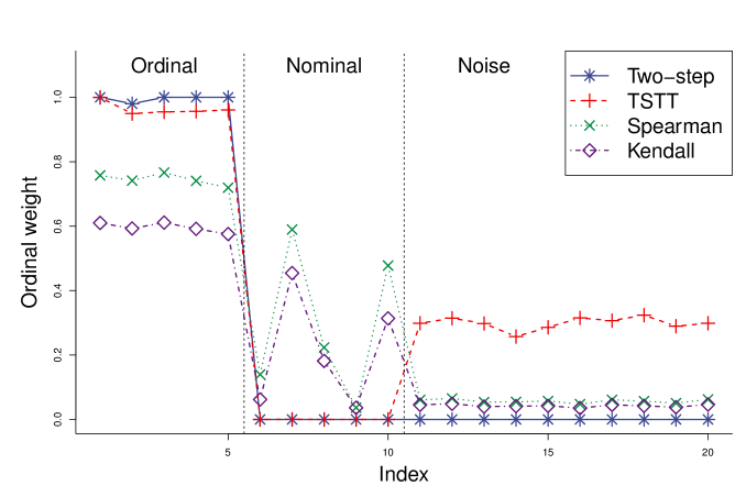
Figure 2: Averaged ordinal weights for the first $20$ variables (The patterns for other $p-20$ variables are similar to the noise variables shown here). See Section 3.5.

4 Theory

We begin with introducing notation for matrix indexing and matrix norms. For a matrix $V\in\mathbb{R}^{m\times n}$, $V_{i,:}$ denotes the $i$th row of $V$ and $V_{:,j}$ denotes the $j$th column of $V$. For index sets $I\subset\{1,2,\dots,m\}$ and $J\subset\{1,2,\dots,n\}$, $V_{I,:}$ is a submatrix of $V$ with rows indexed by $I$. We also denote $V_{I}=V_{I,:}$ if there is no confusion. $V_{I,J}$ denotes the submatrix of $V$ with row indices $I$ and column indices $J$. Matrix norms $\|\cdot\|_{\infty}$ and $\|\cdot\|_{\infty,2}$ are defined as $\|V\|_{\infty}=\max_{1\leq i\leq m}\|V_{i,:}\|_{1}$ and $\|V\|_{\infty,2}=\max_{1\leq i\leq m}\|V_{i,:}\|_{2}$. Next, for two sequences $\{a_{n}\}$ and $\{b_{n}\}$, we write $a_{n}\lesssim b_{n}$ if there exists a positive constant $C>0$ and $n_{0}\in\mathbb{N}$ such that $a_{n}\leq Cb_{n}$ for all $n\geq n_{0}$. We denote $a_{n}\asymp b_{n}$ if $a_{n}\lesssim b_{n}$ and $b_{n}\lesssim a_{n}$.

In this section, we give theoretical results for SOBL. Theorems presented in this section provide us with an understanding of the role of parameters $(\lambda,\eta)$ in SOBL. Under suitable choices of $(\lambda,\eta)$, statistical properties of SOBL such as variable selection property and basis error bounds in terms of $\|\cdot\|_{\infty,2}$ are presented in both non-asymptotic and asymptotic cases.

4.1 Variable selection and basis learning properties

The proposed SOBL (7) takes $(\widehat{\Sigma},\widehat{M})$ as an input. Among the choices of $(\widehat{\Sigma},\widehat{M})$ listed in Table 1, we analyze the choices corresponding to MGSDA (Gaynanova et al., 2016) and MSDA (Mai et al., 2019). Recall that $\Sigma$ and $M$ are estimands of $\widehat{\Sigma}$ and $\widehat{M}$. In MSDA, $\Sigma=\Sigma_{w}$ and $M=[\mu_{2}-\mu_{1},\dots,\mu_{K}-\mu_{1}]$. For MGSDA, $\Sigma=\Sigma_{T}=\Sigma_{w}+\Sigma_{b}$ and $M=\mathbb{E}\widehat{M}$. While all results in this section apply to both choices, we do not present theoretical results corresponding to fastPOI (Jung et al., 2019). This is because our strategy of dealing with mean differences does not directly apply to the eigenvectors of $\widehat{\Sigma}_{b}$.

For the ordinal weights, we use the two-step ordinal weights, discussed in Section 3.3, with $(\theta_{1},\theta_{2})$ defined in Theorem 1. Although $\theta_{1}$ contains population quantities which we do not know in general, Theorem 1 enables us to derive the theoretical results presented in the current section.

For notational convenience, we let $A=J_{disc}$, $A_{1}=J_{disc}^{ord}$, and $A_{2}=J_{disc}\cap J_{ord}^{c}$. Note that in general $A_{2}\neq J_{nom}=J_{md}\cap J_{ord}^{c}$. Under these notation, we introduce population quantities that appear in the theorems. Let us define irrepresentability quantity $\kappa=\|\Sigma_{A^{c}A}(\Sigma_{AA})^{-1}\|_{\infty}$. Next, we define $\phi=\|(\Sigma_{AA})^{-1}\|_{\infty}$, $\delta=\|M\|_{\infty,2}$, $\delta_{1}=\|M_{A_{1}}\|_{\infty,2}$ and $\delta_{2}=\|M_{A_{2}}\|_{\infty,2}$. Let $d=|J_{disc}|$.

The following theorem shows the variable selection property of SOBL. The proof is given in the Appendix.

Theorem 2.

Assume Conditions (C1)-(C3) in Section 3.4 and $\kappa<1$. Let $\widehat{Z}^{ord}_{\eta,\lambda}$ be the SOBL basis with ordinal weights defined in Theorem 1. The following hold for all sufficiently large $N$.

1. Let $\epsilon_{1}\coloneqq\min\left(\frac{1}{\phi},\frac{\lambda(1-\eta\kappa)}{\lambda\phi(1+\eta)+(1+\kappa)(1+\phi\delta)}\right)$. For any $\lambda>0,1\leq\eta<\frac{1}{\kappa}$ and $0<\epsilon<\epsilon_{1}$,

   $$\Pr\left((\widehat{Z}^{ord}_{\eta,\lambda})_{J_{disc}^{c}}=\mathbf{0}\right)\geq 1-\gamma.$$

   Here,

   $$\gamma=Cpd\exp(-\frac{CN\epsilon^{2}}{d^{2}})+2p\exp(-\frac{N\Delta^{2}}{32})+\frac{Cp}{\sqrt{N}\bar{\delta}_{\min}}\exp(-CN\bar{\delta}_{\min}^{2}),$$

   where $C>0$ is a generic constant only depending on $c_{1},c_{2}$ of Condition (C1).

2. Suppose that $\Sigma_{A_{2}A_{2}^{c}}=\mathbf{0}$. Let

   $$\epsilon_{2}\coloneqq\min\bigg{(}\frac{1}{\phi},~{}\frac{\lambda\eta-\delta_{2}}{1+\phi(\delta_{1}-\delta_{2}+\lambda+\lambda\eta)},~{}\frac{\lambda(1-\kappa)}{2\lambda\phi+(1+\phi\delta_{1})(1+\kappa)}\bigg{)}.$$

   For any $\lambda>0$, $\eta>\frac{\delta_{2}}{\lambda}\vee 1$ and $0<\epsilon<\epsilon_{2}$,

   $$\Pr\left((\widehat{Z}^{ord}_{\eta,\lambda})_{(J_{disc}^{ord})^{c}}=\mathbf{0}\right)\geq 1-\gamma.$$

The first part of Theorem 2 states that when $\eta\approx 1$, SOBL successfully screens out variables in $J_{disc}^{c}$ with probability at least $1-\gamma$. SOBL simply becomes a non-ordinal sparse LDA basis learning method when $\eta=1$. For such a special case, the finding of Theorem 2 is equivalent to the variable selection properties appeared in Gaynanova et al. (2016) and Mai et al. (2019). This makes sense since for a small $\eta$, there is no significant difference between ordinal and non-ordinal sparse LDA methods.

The second part of Theorem 2 shows that with a suitably large choice of $\eta$, SOBL only chooses the variables contained in $J_{disc}^{ord}$ and does not select variables in $(J_{disc}^{ord})^{c}$ with high probability. Consider $(\lambda,\eta)$ selected as in the second part of the theorem. The pair $(\lambda,\eta)$ then should satisfy $\lambda\eta>\delta_{2}=\|M_{A_{2}}\|_{\infty,2}$. Note that under the setting of Theorem 2, the penalty coefficient $\lambda_{j}=\lambda\eta^{1-w_{j}}$, for $j\in J_{ord}^{c}$, becomes $\lambda\eta$ with probability at least $1-\gamma$. Thus, in order for $\widehat{Z}^{ord}_{\eta,\lambda}$ to choose only $J_{disc}^{ord}$, one should choose $(\lambda,\eta)$ large so that $\lambda\eta$ is larger than the mean differences of variables in $J_{disc}\cap J_{ord}^{c}$.

Note that the seemingly restrictive assumption $\Sigma_{A_{2}A_{2}^{c}}=\mathbf{0}$ in the second part of the theorem is only for simplicity. In fact, in order for the probability to converge to 1, it is enough to set $\Sigma_{A_{2}A_{2}^{c}}$ sufficiently small and converges to $\mathbf{0}$ with a suitable order of convergence with respect to $N,p\to\infty$. To select the ordinal discriminant variables properly, we need that the variables of $A_{2}=J_{disc}\cap J_{ord}^{c}$ are (nearly) uncorrelated with the other variables.

Based on Theorem 2, the next theorem states a non-asymptotic bound for the error of the estimated SOBL basis $\widehat{Z}_{\eta,\lambda}^{ord}$ in estimation of the population discriminant basis $\Psi$.

Theorem 3.

Assume Conditions (C1)-(C3) in Section 3.4 and $\kappa<1$. Let $\widehat{Z}^{ord}_{\eta,\lambda}$ be the SOBL basis with ordinal weights defined in Theorem 1. The following hold for all sufficiently large $N$.

1. For any $\lambda>0$, $1<\eta<\frac{1}{\kappa}$ and $0<\epsilon<\min\left(\epsilon_{1},\frac{1}{2\phi},\frac{2\lambda\eta}{1+\phi\delta}\right)$,

   $$\Pr(\|\widehat{Z}^{ord}_{\eta,\lambda}-\Psi\|_{\infty,2}<6\phi\eta\lambda)\geq 1-\gamma$$

2. Suppose that $\Sigma_{A_{2}A_{2}^{c}}=\mathbf{0}$. For any $\lambda>0$, $\eta>\frac{\delta_{2}}{\lambda}\vee 1$ and $0<\epsilon<\min\left(\epsilon_{2},\frac{1}{2\phi},\frac{2\lambda}{1+\phi\delta_{1}}\right)$,

   $$\Pr(\|(\widehat{Z}^{ord}_{\eta,\lambda})_{J_{disc}^{ord}}-\Psi_{J_{disc}^{ord}}\|_{\infty,2}\leq 6\phi\lambda)\geq 1-\gamma.$$

   In addition, we have that $\|(\widehat{Z}^{ord}_{\eta,\lambda})_{J_{disc}^{c}}-\Psi_{J_{disc}^{c}}\|_{\infty,2}=0$, and $\|(\widehat{Z}^{ord}_{\eta,\lambda})_{A_{2}}-\Psi_{A_{2}}\|_{\infty,2}\leq\phi\delta_{2}$ hold with probability at least $1-\gamma$.

Similar to the case of variable selection, for a small $\eta\approx 1$, $\|\widehat{Z}_{\eta,\lambda}^{ord}-\Psi\|_{\infty,2}$ is less than $\lambda$ up to constant with probability greater than or equal to $1-\gamma$. Similar results were observed in sparse multiclass LDA contexts (Gaynanova et al., 2016; Mai et al., 2019).

The second part of Theorem 3 reveals that the SOBL basis restricted to $J_{disc}^{ord}$ estimates $\Psi_{J_{disc}^{ord}}$ with the error bounded by a multiple of $\lambda$. In this case, however, SOBL discards the variables in $A_{2}=J_{disc}\cap J_{ord}^{c}$, which also affects the population discriminant subspace. In this perspective, classification performance may decline when we use SOBL rather than sparse LDA. On the other hand, if inherent ordinal signals are strong enough, then the classification performance of SOBL is comparable to sparse LDA, while SOBL selects significantly fewer variables than sparse LDA. In the real data example of Section 5.4, we demonstrate that the sparse and ordinal basis, estimated by SOBL, provides better interpretability while showing comparable classification performances.

4.2 Asymptotic analysis

For asymptotic analysis, we assume that $p,d$ may grow as $N\to\infty$. We also assume that the tuning parameters $\lambda\equiv\lambda_{N}$ and $\eta\equiv\eta_{N}$ depend on the sample size $N$. To guarantee consistency of $\widehat{Z}_{\eta_{N},\lambda_{N}}^{ord}$, it is necessary to ensure both $\lambda_{N}\to 0$ and $\gamma\to 0$ as $N\to\infty$; see the probability statements in Theorem 3.

In Theorems 2 and 3, the free parameter $\epsilon$ should be located in $(0,\epsilon_{1})$ or $(0,\epsilon_{2})$. Since $\epsilon_{1},\epsilon_{2}\lesssim\lambda_{N}$ in the theorem, it is also true that $\epsilon\lesssim\lambda_{N}$. To minimize the first term of $\gamma$, $pd\exp(-CN\epsilon^{2}/d^{2})$, we should choose $\epsilon\asymp\lambda_{N}$. So, $pd\exp(-CN\lambda_{N}^{2}/d^{2})\to 0$ is sufficient to make the first term of $\gamma$ tend to $0$. Thus, $\lambda_{N}$ must decrease to $0$ in a moderate speed with respect to the asymptotic conditions of $(N,p,d)$. In a similar manner, we need asymptotic conditions on $\Delta$ and $\bar{\delta}_{\min}$ for the second and third terms of $\gamma$.

To develop asymptotic versions of Theorem 2 and 3, we use the following asymptotic conditions.

• $\frac{\log(pd)d^{2}}{N}\to 0$.

• $\lambda_{N}\gtrsim\left(\frac{\log(pd)d^{2}}{N}\right)^{\frac{1-\alpha}{2}}$ for some $\alpha\in(0,1)$ and $\lambda_{N}\to 0$.

• $\Delta\wedge\bar{\delta}_{\min}\gtrsim\frac{1}{d}$.

• $\lim_{N\to\infty}\eta_{N}\lambda_{N}>C\delta_{2}$ for some constant $C>1$.

Note that (AC1) and (AC2) also appear in the asymptotic results of sparse LDA (Mai et al., 2012; Gaynanova et al., 2016; Mai et al., 2019). Condition (AC1) implies that $p$ may grow faster than any polynomial order of $N$ (Mai et al., 2012). (AC2) controls the error bound for the estimated basis with probability tending to $1$. Condition (AC3) is needed to guarantee consistency of the two-step ordinal weights. We note that $\Delta\wedge\bar{\delta}_{\min}\to 0$ is allowed in (AC3) if $d\to\infty$. Finally, (AC4) is only required when the variable selection is targeted at $J_{disc}^{ord}$, as in the second part of Theorem 2.

With conditions (AC1)-(AC4), SOBL enjoys consistency in variable selection and of the estimated basis, as shown in the following two corollaries.

Corollary 4.

Suppose condition (C1) and asymptotic conditions (AC1)-(AC3) hold. Assume that $\kappa<1$ and $1<\eta_{N}<\frac{1}{\kappa}$ for any $N$. Then, we have $\Pr\left((\widehat{Z}^{ord}_{\eta,\lambda})_{J_{disc}^{c}}=0\right)\to 1$ and $\Pr\left(\|\widehat{Z}^{ord}_{\eta,\lambda}-\Psi\|_{\infty,2}<\varepsilon\right)\to 1$ for any $\varepsilon>0$.

Corollary 5.

Suppose condition (C1) and asymptotic conditions (AC1)-(AC4) hold. Assume that $\kappa<1$ and $\Sigma_{A_{2}A_{2}^{c}}=\mathbf{0}$ for any $N$. Then, we have $\Pr\left((\widehat{Z}^{ord}_{\eta,\lambda})_{(J_{disc}^{ord})^{c}}=0\right)\to 1$ and $\Pr\left(\|(\widehat{Z}^{ord}_{\eta,\lambda})_{J_{disc}^{ord}}-\Psi_{J_{disc}^{ord}}\|_{\infty,2}<\varepsilon\right)\to 1$ for any $\varepsilon>0$.

5 Numerical studies

In this section, we numerically demonstrate the performance of the proposed sparse ordinal basis learning (SOBL), with $(\widehat{\Sigma},\widehat{M})$ chosen as in Table 1. Each of these choices will be refereed to as ord-MGSDA, ord-MSDA, and ord-fastPOI, respectively. We use the two-step ordinal weights defined in Section 3.3 with $(\hat{\theta}_{1},\hat{\theta}_{2})$ given by (15). Once we obtain the SOBL basis $\widehat{Z}_{\eta,\lambda}^{ord}$, one can conduct classification and visualization using the data projected on the low dimensional subspace $\mathcal{C}(\widehat{Z}_{\eta,\lambda}^{ord})$. For numerical stability, we add a small $\epsilon I_{p}$ to the $\widehat{\Sigma}$ and use the orthogonal basis $\hat{Q}$ obtained from the QR decomposition of $\widehat{Z}_{\eta,\lambda}^{ord}$ as done in Jung et al. (2019). Classical multiclass LDA rule is then fitted to $(\mathbf{X}\hat{Q},\mathbf{Y})$ as in the sparse multiclass LDA literature (Mai et al., 2019; Jung et al., 2019). For visualization, a scatter plot can be produced based on the projected dataset $(\mathbf{X}\hat{Q},\mathbf{Y})$.

5.1 Tuning parameter selection scheme

A usual choice for the tuning parameters is obtained by a cross-validation on a predetermined $(\lambda,\eta)$ grid. However, as we will see in our simulation results, choosing the parameter $(\lambda,\eta)$ on the two-dimensional grid that maximizes the classification accuracy typically results in selecting more variables than $J_{disc}^{ord}$. To capture $J_{disc}^{ord}$ properly, we propose a two-step tuning procedure:

1. Fix $\eta=1$. Choose the best $\tilde{\lambda}$ on a fine grid $(0,\lambda_{\max})$ with respect to the classification accuracy.

2. Fix $\lambda=\tilde{\lambda}$ and fit $\widehat{Z}_{\eta,\tilde{\lambda}}^{ord}$ for a sequence of $\eta$, ranging from $1$ to $\eta_{\max}$. Let $\tilde{\eta}$ be the value satisfying that $\widehat{Z}_{\eta,\lambda}^{ord}$ does not change for $\eta\geq\tilde{\eta}$. Choose $\eta=\tilde{\eta}$.

We set $\lambda_{\max}=\|\widehat{M}\|_{\infty,2}$, and $\eta_{\max}=2(\|\widehat{M}\|_{\infty,2}/\tilde{\lambda}+1)$. If $\lambda>\lambda_{\max}$ then $\widehat{Z}_{1,\lambda}^{ord}$ becomes $0$ (Jung et al., 2019). The choice of $\eta_{\max}$ comes from the assumption for $\eta$ in the second part of Theorem 2, that is, $\eta>\delta_{2}/\lambda\vee 1$. The basic idea of the two-step tuning procedure is based on the second part of Theorem 2: To choose $J_{disc}^{ord}$ properly, we need large enough $\eta$.

How the two-step tuning procedure works is illustrated with a toy data in Figure 3. The data are generated from the simulation setting of Section 5.3, in which we set $p=200$ and $(n_{1},n_{2},n_{3})=(100,100,100)$. In this data set, $\tilde{\lambda}=0.277$ (with $\eta=1$ fixed) provides the largest cross-validated classification accuracy. With $\tilde{\lambda}$ fixed, we observe that as $\eta$ increasing, non-ordinal variables tend to “die” while the ordinal discriminant variables in $J_{disc}^{ord}$ resist and stay included in the estimate for larger $\eta$. The left panel of Figure 3 shows that as $\eta$ increases, $\|(\widehat{Z}_{\eta,\tilde{\lambda}}^{ord})_{j,:}\|_{2}$ decreases to $0$ for $j\in J_{ord}^{c}$. Remarkably, one of the two variables belonging to $J_{disc}^{ord}$ was not selected for small values of $\eta$, then became included for larger $\eta>2$. After all non-ordinal and noise variables are removed at $\eta=\tilde{\eta}=2.26$, there is no more change in the estimate as $\eta$ keeps increasing. This is because the penalty coefficient for ordinal variables, $\lambda_{j}=\tilde{\lambda}$, is fixed throughout the second tuning step, while the penalty coefficient for non-ordinal variables, $\lambda_{j}=\tilde{\lambda}\eta$, grows as $\eta$ increases. Thus, once the non-ordinal variables become zero, larger penalty simply does not make a difference in estimates. This two-step tuning procedure aims to select $J_{disc}^{ord}$, albeit making compromises on classification accuracy, if the ordinal signal strength is weak. As can be seen in the scatter plots in Figure 3, the data projected on the ordinal basis $\widehat{Z}_{\tilde{\eta},\tilde{\lambda}}^{ord}$ (shown in the right panel) clearly show an ordinal group tendency in the first direction, while the data projected on $\widehat{Z}_{1,\tilde{\lambda}}^{ord}=\widehat{Z}_{\tilde{\lambda}}$ in the middle panel do not reflect the order.

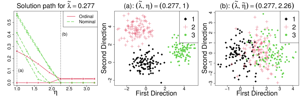
Figure 3: The left panel shows a solution path for $\tilde{\lambda}=0.277$ of ord-fastPOI with respect to $\eta$. Each line denotes $\|(\widehat{Z}_{\eta,\tilde{\lambda}}^{ord})_{j,:}\|_{2}$ for $j\in J_{md}$. Non-ordinal mean-difference variables are labeled “nominal.” The middle and right panels show corresponding projected scatter plots for (a) and (b) in the first plot.

5.2 Competing methods

We compare variable selection and classification performances of SOBL to the methods of Ma and Ahn (2021) and Archer et al. (2014). Ma and Ahn (2021) proposed feature-weighted ordinal classification (FWOC) which solves the sparse LDA objective (5) with $\widehat{\Sigma}$ adjusted by ordinal weights. The FWOC is also a sparse basis learning method. In Archer et al. (2014), several types of penalized ordinal logistic regression models are proposed. Among those, we choose to compare with a penalized cumulative logistic model (PCLM), which estimates the coefficient vector $\beta\in\mathbb{R}^{p}$ maximizing a penalized likelihood $L(\alpha,\beta)-\lambda\sum_{j=1}^{p}|\beta_{j}|$ under the cumulative logit model: $\mbox{logit}(\mbox{Pr}\left(Y\leq j\>|\>\mathbf{x}\right))=\alpha_{j}+\mathbf{x}^{T}\beta$. We follow tuning procedures as in the original papers.

5.3 Variable selection performance

The variable selection property of the proposed method is demonstrated with a simulation study.

To examine whether the SOBL selects the variables in $J_{disc}^{ord}$, rather than those in $J_{disc}$, we use the mean structure appeared in Example 1, and a block diagonal covariance structure to guarantee $J_{ord}\nsubseteq J_{disc}$. For $p\in\{200,800\}$ and $|J_{md}|=8$, we set

$$[\mu_{1},\mu_{2},\mu_{3}]=\left[\begin{array}[]{cccc:cccc:c}0.5&0&0&0&0&0&0&0&\mathbf{0}_{p-8}^{T}\\ 1&0.5&1&-1&3&2&-1&-0.5&\mathbf{0}_{p-8}^{T}\\ 1.5&1.0&2&-1.5&2&-0.5&2&3&\mathbf{0}_{p-8}^{T}\end{array}\right]^{T},$$

$$\Sigma=\begin{pmatrix}\Sigma_{s}&\mathbf{0}_{8,\>p-8}\\ \mathbf{0}_{p-8,\>8}&\Sigma_{p-8}\end{pmatrix},\quad\Sigma_{j}=\frac{1}{2}(I_{j}+1_{j}1_{j}^{T})\ \mbox{for}\ j\in\mathbb{N}.$$

For the $g$th group, we generate random samples from $N_{p}(\mu_{g},\Sigma)$. In this case, $J_{ord}=\{1,2,3,4\}$, $J_{disc}^{ord}=\{3,4\}$ and $J_{disc}=\{3,4,5,6,7,8\}$. We repeat 100 times to generate $(n_{1},n_{2},n_{3})=(50,50,50)$ random samples for train set and generate test set with the same sample sizes. We conduct both the two-step tuning procedure and 5-fold cross-validation procedure on a $(\lambda,\eta)$ grid to compare the difference between the two tuning procedures. Also, we fit sparse multiclass LDA methods for a baseline comparison. After fitting, we measure variable selection performance on the fitted model and report classification accuracy with respect to $l_{0},l_{1}$ and $l_{2}$ losses. Here, the $l_{k}$ loss, for $k=0,1,2$, is given by $\frac{1}{N}\sum_{i=1}^{N}|\hat{y}_{i}-y_{i}|^{k}$ where $\hat{y}_{i}$ is an estimated class of the $i$th observation in the test set.

$p$	Index set	ord-MGSDA	ord-MGSDA-grid	MGSDA	FWOC	PCLM
$200$	$|\widehat{D}|$	2.35(0.067)	5.47(0.098)	6.40(0.287)	15.9(2.83)	18.0(8.88)
	$|\widehat{D}\cap A|$	2.31(0.065)	5.40(0.085)	5.37(0.052)	5.41(0.071)	5.79(0.856)
	$|\widehat{D}\cap A_{1}|$	1.98(0.014)	1.57(0.050)	1.36(0.050)	1.32(0.053)	2.00(0)
	$|\widehat{D}\cap A^{c}|$	0.04(0.020)	0.07(0.038)	1.03(0.256)	10.5(2.78)	12.2(8.68)
	$|\widehat{D}\cap A_{1}|/|\widehat{D}|$	0.892(0.018)	0.286(0.007)	0.221(0.006)	0.181(0.009)	0.142(0.008)
$800$	$|\widehat{D}|$	2.39(0.066)	5.45(0.081)	9.65(3.030)	33.2(9.96)	15.6(9.05)
	$|\widehat{D}\cap A|$	2.36(0.063)	5.42(0.074)	5.27(0.057)	5.55(0.077)	5.18(0.809)
	$|\widehat{D}\cap A_{1}|$	1.99(0.010)	1.60(0.049)	1.29(0.048)	1.44(0.054)	2.00(0)
	$|\widehat{D}\cap A^{c}|$	0.03(0.022)	0.03(0.022)	4.38(3.030)	27.6(9.91)	10.4(8.83)
	$|\widehat{D}\cap A_{1}|/|\widehat{D}|$	0.882(0.018)	0.291(0.007)	0.213(0.007)	0.203(0.010)	0.170(0.008)

Table 2: Variable selection performances of each method with 100 repetitions on simulation settings. Averaged measures are presented. Values in parentheses are standard errors. Here, $A$ denotes $J_{disc}$ and $A_{1}$ denotes $J_{disc}^{ord}$.

Table 2 shows variable selection performance results. We only report SOBL and sparse LDA based on MGSDA as the results from other methods are similar. The index set of selected variables of each method is denoted by $\widehat{D}$. Thus, $|\widehat{D}|$ is the number of selected variables. In both $p=200$ and $p=800$, the proposed ord-MGSDA shows the highest ratio of $J_{disc}^{ord}$ in selected variables, $|\widehat{D}\cap A_{1}|/|\widehat{D}|$, among all methods considered. Indeed, ord-MGSDA based on grid search (ord-MGSDA-grid) chooses almost all $J_{disc}$. PCLM always selects all variables in $J_{disc}^{ord}$ but also mistakenly selects too many of $J_{disc}^{c}$. FWOC can not properly select $J_{disc}^{ord}$ and also frequently selects noise variables. We observe that ord-MGSDA-grid selects $J_{disc}$ properly but not $J_{disc}^{ord}$. In contrast, the baseline method, MGSDA, tends to include noise variables in the high dimensional case of $p=800$. With fewer variables selected, ord-MGSDA-grid has a comparable classification performance to MGSDA (with more variables), as shown in Table 3. Among the methods compared in the table, we note that ord-MGSDA shows a poor classification performance. This is because the magnitude of mean difference of ordinal variables is smaller than that of non-ordinal mean-difference variables, in the simulation model. While it appears that classification performance is sacrificed to have the superior variable selection property in SOBL, this is not always the case as we claim in our real data example.

$p$	Metric	ord-MGSDA	ord-MGSDA-grid	MGSDA	FWOC	PCLM
$200$	$l_{0}$	0.262(0.004)	0.012(0.001)	0.008(0.001)	0.010(0.001)	0.140(0.003)
	$l_{1}$	0.265(0.005)	0.017(0.002)	0.011(0.001)	0.015(0.002)	0.140(0.003)
	$l_{2}$	0.273(0.006)	0.028(0.003)	0.018(0.002)	0.026(0.003)	0.140(0.003)
$800$	$l_{0}$	0.252(0.004)	0.013(0.001)	0.013(0.005)	0.009(0.001)	0.139(0.003)
	$l_{1}$	0.257(0.004)	0.018(0.002)	0.018(0.005)	0.015(0.002)	0.140(0.003)
	$l_{2}$	0.265(0.005)	0.029(0.003)	0.027(0.006)	0.026(0.003)	0.140(0.003)

Table 3: Classification performances of each method with 100 repetitions on simulation settings. Averaged measures are presented. Values in parentheses are standard errors.

5.4 Real data analysis

We apply SOBL to two high-dimensional gene expression data sets and compare the performance of SOBL with those of competing methods. The first data set is the primary human Glioma data set (Sun et al., 2006). Glioma is a type of tumor that starts in the brain and spine and has severe prognosis results for patients. In the glioma data set, each observation has an ordinal class among ‘Normal’ $\prec$ ‘Grade II’ $\prec$ ‘Grade III’ $\prec$ ‘Grade IV.’ The predictor $X$ is a preprocessed gene expression data with $p=54,612$. The sample sizes of the four classes are $(n_{1},n_{2},n_{3},n_{4})=(23,45,31,81)$, with $N=180$. The second gene expression data is B-cell Acute Lymphoblastic Leukemia (ALL) data set, provided by Chiaretti et al. (2004) and maintained by Li (2022). In ALL data set, we have $X\in\mathbb{R}^{12,625}$ and each observation belongs to one of the ordinal classes $B_{1}\prec B_{2}\prec B_{3}\prec B_{4}$ where $(n_{1},n_{2},n_{3},n_{4})=(19,36,23,12)$. The total sample size of ALL data set is $N=90$. The purposes of analysis are to predict the class labels based on the predictors and to conduct variable selection.

First, we compare $l_{0},l_{1},l_{2}$ losses and the number of selected variables. We split the whole data set into train and test sets by 4:1, and then further split the train set into the fitting and validation sets by 3:1. That is, we randomly divide the data set into three parts with fitting:validation:test $=$ 3:1:1. As in the sparse multiclass LDA literature, we first apply screening. We chose 1,000 variables in Glioma data analysis and 500 variables in ALL data analysis by MV-SIS, a screening method for high dimensional classification problem (Cui et al., 2015), to rule out irrelevant variables at the training step. On the train set, we utilize the fitting and validation sets to tune and fit the best model on the whole train set. Finally, we measure losses on the test set and record the number of selected variables for each method. This is repeated for 100 times, and Table 4 collects averaged performance measures with standard error.

Data set	Metric	ord-MGSDA	MGSDA	ord-fastPOI	fastPOI	FWOC	PCLM
Glioma	$l_{0}$	0.385(0.012)	0.596(0.013)	0.378(0.006)	0.356(0.007)	0.328(0.007)	0.362(0.007)
	$l_{1}$	0.583(0.027)	1.02(0.025)	0.525(0.012)	0.511(0.012)	0.456(0.013)	0.453(0.009)
	$l_{2}$	1.07(0.070)	2.09(0.061)	0.866(0.031)	0.899(0.031)	0.775(0.031)	0.648(0.018)
	$|\widehat{D}|$	44.2(7.75)	228.0(9.96)	53.6(12.2)	79.7(18.4)	334.0(33.7)	70.9(3.01)
ALL	$l_{0}$	0.445(0.012)	0.434(0.011)	0.503(0.012)	0.508(0.010)	0.450(0.011)	0.476(0.021)
	$l_{1}$	0.555(0.016)	0.540(0.014)	0.625(0.017)	0.641(0.015)	0.561(0.014)	0.549(0.024)
	$l_{2}$	0.779(0.029)	0.764(0.026)	0.880(0.033)	0.928(0.032)	0.795(0.028)	0.694(0.037)
	$|\widehat{D}|$	18.7(1.52)	49.5(3.92)	14.7(1.68)	101.0(15.3)	140.0(14.5)	39.9(2.9)

Table 4: Classification and variable selection performances of each method with 100 repetitions on real data sets. Averaged measures are presented. Values in parentheses are standard errors.

Remarkably, in both data sets, SOBL methods (ord-MGSDA and ord-fastPOI) select fewer variables than corresponding sparse multiclass LDA methods while maintaining similar or lower $l_{0}$ values than sparse LDA methods. It is notable that in the case of the glioma data set, ord-fastPOI reports a smaller value of $l_{2}$ loss than fastPOI even though fastPOI has a lower $l_{0}$ loss than ord-fastPOI. In glioma dataset, FWOC performs best in terms of classification performance with respect to $l_{0}$ loss, but FWOC selects too many variables which makes interpretations somewhat clumsy. PCLM is best in terms of the $l_{2}$ loss in both cases. However, PCLM also selects significantly more variables than ord-MGSDA and ord-fastPOI.

We further take a look at the difference between the selected variables of SOBL and non-ordinal sparse multiclass LDA methods. For this, we fit ord-MGSDA, ord-fastPOI, MGSDA, and fastPOI with 5-fold cross-validation based on all sample. For SOBL, we select $(\lambda,\eta)$ by the two-step tuning procedure proposed in Section 5.1. After fitting, we plot the sample group means of selected variables, in Figures 4 and 5.

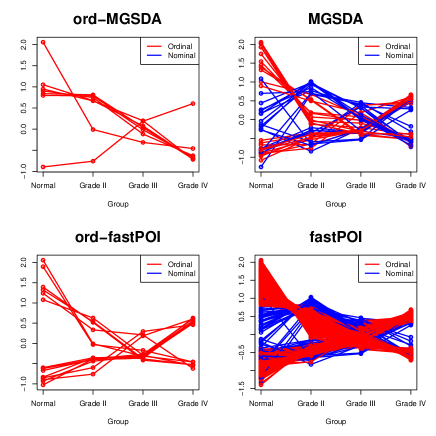
Figure 4: The class mean plots of selected variables in Glioma data. The y-axis shows sample mean values and the x-axis denotes the ordered class labels. The proposed Ord-MGSDA (and ord-fastPOI) selects 7 (and 14, respectively) ordinal variables with no nominal (non-ordinal) variables selected at all. In contrast, MGSDA selects 21 ordinal variables and 21 non-ordinal variables; fastPOI selects 496 ordinal variables and 55 non-ordinal variables.

Figure 5: The class mean plots of selected variables in ALL data. The proposed Ord-MGSDA (and ord-fastPOI) selects 30 (and 55, respectively) ordinal variables with no nominal (non-ordinal) variables selected at all. In contrast, MGSDA selects 12 ordinal variables and 60 non-ordinal variables; fastPOI selects 444 ordinal variables and 56 non-ordinal variables.

We observe that SOBL selects only ordinal variables while sparse multiclass LDA methods select both ordinal and non-ordinal variables. As in the simulation results presented in Section 5.3, we may interpret that SOBL selects variables in the ordinal discriminant variable set, $J_{disc}^{ord}$, which is strictly contained in discriminant features $J_{disc}$. In Table 4, we have already observed that, contrary to the classification performance reported in the simulations, SOBL has comparable classification power to non-ordinal sparse LDA. This reflects that ordinal discriminant variables in Glioma and ALL data sets have strong enough signals for classification and SOBL indeed chooses such ordinal discriminant variables.

Appendix A Proof of Theorem 1

We proceed the proof with proving the result for univariate case and then aggregate the results of all variables. We propose some lemmas that describe tail probability of two types of Kendall’s rank correlations $\hat{\tau}$ and $\tilde{\tau}$ introduced in Section 3.3.

First, we introduce some concentration results introduced at Vershynin (2018).

Theorem 6 (McDiamard’s inequality).

Let $X_{1},\dots,X_{n}$ be independent random elements having values on $\mathcal{X}$. Let $f:\mathcal{X}^{n}\to\mathbb{R}$ be a measurable function. Assume that for any index $i\in\{1,\dots,n\}$ and any $x_{1},\dots,x_{n},x_{i}^{\prime}\in\mathcal{X}$ we have

$$|f(x_{1},\dots,x_{i-1},x_{i},x_{i+1},\dots,x_{n})-f(x_{1},\dots,x_{i-1},x_{i}^{\prime},x_{i+1},\dots,x_{n})|\leq c_{i}$$

for some constant $c_{i}>0$. Then, for any $t>0$, we have

$$\mbox{Pr}\left(f(X)-\mathbb{E}f(X)\geq t\right)\leq\exp\left(-\frac{2t^{2}}{\sum_{i=1}^{n}c_{i}^{2}}\right)$$

where $X=(X_{1},\dots,X_{n})$.

Lemma 7 (Tail of the normal distribution).

Let $Z\sim N(0,1)$. Then for all $t>0$, we have

$$\mbox{Pr}\left(Z\geq t\right)\leq\frac{1}{t}\cdot\frac{1}{\sqrt[]{2\pi}}e^{-t^{2}/2}$$

Through Lemmas 8 and 9, we consider an univariate setting. We assume the gaussian model: Let $\mu_{g}\in\mathbb{R}$ be group mean of class $g\in\{1,\dots,K\}$ and $\sigma$ be a standard deviation. Then $(X,y)$ follows $X~{}|~{}y=g\overset{i.i.d.}{\sim}N(\mu_{g},\sigma^{2})$, for $g=1,\dots,K$. We have total $N$ independent samples of $(X_{i},y_{i})_{i=1}^{N}$. We recall that $y_{1},\dots,y_{N}$ are fixed and deterministic. Denote the group mean by $\hat{\mu}_{g}=\frac{1}{n_{g}}\sum_{y_{i}=g}X_{i}$. Recall that

1. $\hat{\tau}=\frac{2}{N(N-1)}\sum_{1\leq i<j\leq N}\mbox{sign}(X_{j}-X_{i})\mbox{sign}(y_{j}-y_{i})$,

2. $\tilde{\tau}=\frac{2}{K(K-1)}\sum_{1\leq i<j\leq K}\mbox{sign}(\hat{\mu}_{j}-\hat{\mu}_{i})$.

Lemma 8.

For any $\mu_{1},\dots,\mu_{K}$, we have

$$\mbox{Pr}\left(|\hat{\tau}-\mathbb{E}\hat{\tau}|\geq t\right)\leq 2\exp\left(-\frac{Nt^{2}}{8}\right).$$ (16)

Proof.

For any $i=1,\dots,N$ and for any $x_{1},\dots,x_{N},x_{i}^{\prime}\in\mathbb{R}$, Then we have

$$|\hat{\tau}(x_{1},\dots,x_{i-1},x_{i},x_{i+1},\dots,x_{N})-\hat{\tau}(x_{1},\dots,x_{i-1},x_{i}^{\prime},x_{i+1},\dots,x_{N})|$$

$$\leq\frac{2}{N(N-1)}\sum_{k\neq i}|\mbox{sign}(x_{i}-x_{k})-\mbox{sign}(x_{i}^{\prime}-x_{k})|$$

$$\leq\frac{2}{N(N-1)}\cdot 2(N-1)=\frac{4}{N}.$$

By McDiamard’s inequality (Theorem 6), we have the result. ∎

Lemma 9.

Suppose that $\mu_{1},\dots,\mu_{K}$ are all different. Also, assume that $c_{1}\leq n_{g}/N\leq c_{2}$ for some fixed constants $c_{1},c_{2}>0$ for all $g=1,\dots,K$. Let

$$\tau^{o}=\frac{2}{K(K-1)}\sum_{1\leq i<j\leq K}I(\mu_{i}<\mu_{j})-I(\mu_{i}>\mu_{j})$$

and $\delta_{\min}=\min_{1\leq i<j\leq K}|\delta_{ij}|$ where $\delta_{ij}=(\mu_{j}-\mu_{i})/\sigma$. Then

$$|\mathbb{E}\tilde{\tau}-\tau^{o}|\leq\frac{C_{1}}{\sqrt{N}\delta_{\min}}e^{-C_{2}N\delta_{\min}^{2}},$$

where $C_{1},C_{2}>0$ are generic constants which depends only on $c_{1},c_{2}$.

Proof.

Clearly, $\hat{\mu}_{g}\sim N(\mu_{g},\frac{\sigma^{2}}{n_{g}})$ and $\hat{\mu}_{1},\dots,\hat{\mu}_{K}$ are independent. Since $\mathbb{E}\mbox{sign}(\hat{\mu}_{j}-\hat{\mu}_{i})=1-2\Phi\left(-\sqrt{n_{ij}}\delta_{ij}\right)$, where $n_{ij}=(n_{i}^{-1}+n_{j}^{-1})^{-1}$ and $\Phi$ is the distribution function of $N(0,1)$, we have

$$\mathbb{E}\tilde{\tau}=\frac{2}{K(K-1)}\sum_{1\leq i<j\leq K}1-2\Phi\left(-\sqrt{n_{ij}}\delta_{ij}\right).$$

Let us denote $\tau_{ij}=1-2\Phi\left(-\sqrt{n_{ij}}\delta_{ij}\right)$. For $i<j$, consider the two cases of $\mu_{i}<\mu_{j}$ and $\mu_{i}>\mu_{j}$. If $\mu_{i}<\mu_{j}$ then by Lemma 7,

$$|\tau_{ij}-1|=2\mbox{Pr}\left(Z>\sqrt{n_{ij}}\delta_{ij}\right)\leq\frac{2}{\sqrt{2\pi}}\frac{1}{\sqrt{n_{ij}}\delta_{ij}}e^{-\frac{1}{2}n_{ij}\delta_{ij}^{2}}.$$

If $\mu_{i}>\mu_{j}$ then $\delta_{ij}<0$. Again by Lemma 7, we get

$$|\tau_{ij}+1|=2|1-\Phi(-\sqrt{n_{ij}}\delta_{ij})|\leq\frac{2}{\sqrt{2\pi}}\frac{1}{\sqrt{n_{ij}}|\delta_{ij}|}e^{-\frac{1}{2}n_{ij}\delta_{ij}^{2}}.$$

Then

$$|\mathbb{E}\tilde{\tau}-\tau^{o}| \leq\frac{2}{K(K-1)}\left\{\sum_{\begin{subarray}{c}i<j,\\ \mu_{i}<\mu_{j}\end{subarray}}|\tau_{ij}-1|+\sum_{\begin{subarray}{c}i<j,\\ \mu_{i}>\mu_{j}\end{subarray}}|\tau_{ij}+1|\right\}$$

$$\leq\frac{2}{K(K-1)}\sum_{1\leq i<j\leq K}\frac{2}{\sqrt{2\pi}}\frac{1}{\sqrt{n_{ij}}|\delta_{ij}|}e^{-\frac{1}{2}n_{ij}\delta_{ij}^{2}}$$

$$\leq\frac{C_{1}}{\sqrt{N}\delta_{\min}}e^{-C_{2}N\delta_{\min}^{2}},$$

where $C_{1}=4/\sqrt{\pi c_{1}}$ and $C_{2}=c_{1}/4$. ∎

Lemma 10.

Assume the same setting of Lemma 9. Then for any $t>0$,

$$\mbox{Pr}\left(|\tilde{\tau}-\mathbb{E}\tilde{\tau}|>t\right)\leq CK^{2}\left(e^{-C\sqrt{N}\delta_{\min}\exp(CN\delta_{\min}^{2})t}+\frac{1}{\sqrt{N}\delta_{\min}}e^{-CN\delta_{\min}^{2}}\right)$$

where $C>0$ is a generic constant which depends only on $c_{1},c_{2}$.

Proof.

To get the concentration results, we investigate a tail behavior of $W_{ij}\coloneqq\mbox{sign}(\hat{\mu}_{j}-\hat{\mu}_{i}).$ From the proof of Lemma 9, we have $\mathbb{E}W_{ij}=1-2\Phi\left(-\sqrt{n_{ij}}\delta_{ij}\right).$ Then for any $t>0$,

$$\mbox{Pr}(|W_{ij}-\mathbb{E}W_{ij}|>t)$$

$$=\mbox{Pr}(|W_{ij}-\mathbb{E}W_{ij}|>t~{}|~{}\hat{\mu}_{j}>\hat{\mu}_{i})\mbox{Pr}(\hat{\mu}_{j}>\hat{\mu}_{i})$$

$$~{}+\mbox{Pr}(|W_{ij}-\mathbb{E}W_{ij}|>t~{}|~{}\hat{\mu}_{j}<\hat{\mu}_{i})\mbox{Pr}(\hat{\mu}_{j}<\hat{\mu}_{i})$$

$$=I(2\Phi(-\sqrt{n_{ij}}\delta_{ij})>t)\Phi(\sqrt{n_{ij}}\delta_{ij})+I(2\Phi(\sqrt{n_{ij}}\delta_{ij})>t)\Phi(-\sqrt{n_{ij}}\delta_{ij})$$

$$=\Phi(\sqrt{n_{ij}}|\delta_{ij}|)I(2\Phi(-\sqrt{n_{ij}}|\delta_{ij}|)>t)+\Phi(-\sqrt{n_{ij}}|\delta_{ij}|)I(2\Phi(\sqrt{n_{ij}}|\delta_{ij}|)>t)$$ (17)

An upper bound of (17) is given as follows:

$$\mbox{Pr}(|W_{ij}-\mathbb{E}W_{ij}|>t) \leq\Phi(\sqrt{n_{ij}}|\delta_{ij}|)I(2\Phi(-\sqrt{n_{ij}}|\delta_{ij}|)>t)+\Phi(-\sqrt{n_{ij}}|\delta_{ij}|)$$

$$\leq 2e^{-c_{ij}t}+\frac{1}{|\delta_{ij}|\sqrt{2\pi n_{ij}}}e^{-\frac{1}{2}\delta_{ij}^{2}n_{ij}}$$

where $c_{ij}=\frac{\ln 2}{2\Phi(-\sqrt{n_{ij}}|\delta_{ij}|)}$. The first term of the last inequality is derived from the fact that the function $f(t)=2\exp(-c_{ij}t)$ pass through the points $(0,2)$, $(2\Phi(-\sqrt{n_{ij}}|\delta_{ij}|),1)$ and $f$ locates above then $\Phi(\sqrt{n_{ij}}|\delta_{ij}|)I(2\Phi(-\sqrt{n_{ij}}|\delta_{ij}|)>t)$ as a function of $t\in[0,\infty)$. The second term comes from the tail bound of the standard normal distribution, Lemma 7. To further bound $e^{-c_{ij}t}$, again by Lemma 7, we get

$$c_{ij}\geq\sqrt{\frac{\pi}{2}}\ln 2\cdot\sqrt{n_{ij}}|\delta_{ij}|e^{\frac{1}{2}n_{ij}\delta_{ij}^{2}}.$$

Thus, we have

$$\mbox{Pr}(|W_{ij}-\mathbb{E}W_{ij}|>t) \leq 2e^{-c_{ij}t}+\frac{1}{\delta_{ij}\sqrt{2\pi n_{ij}}}e^{-\frac{1}{2}\delta_{ij}^{2}n_{ij}}$$

$$\leq 2e^{-C\sqrt{N}\delta_{\min}\exp(CN\delta_{\min}^{2})t}+\frac{C}{\sqrt{N}\delta_{\min}}e^{-CN\delta_{\min}^{2}},$$ (18)

where $C>0$ is a generic constant only depending on $c_{1},c_{2}$. If $|W_{ij}-\mathbb{E}W_{ij}|\leq t$ for any $1\leq i<j\leq K$, then we have

$$|\tilde{\tau}-\mathbb{E}\tilde{\tau}|\leq\frac{2}{K(K-1)}\sum_{1\leq i<j\leq K}|W_{ij}-\mathbb{E}W_{ij}|\leq\frac{2}{K(K-1)}\cdot\frac{K(K-1)}{2}\cdot t=t.$$

This implies that

$$\mbox{Pr}\left(\bigcap_{1\leq i<j\leq K}\left\{|W_{ij}-\mathbb{E}W_{ij}|\leq t\right\}\right)\leq\mbox{Pr}\left(|\tilde{\tau}-\mathbb{E}\tilde{\tau}|\leq t\right).$$

Finally, by taking complements, the union bound with (18) implies that

$$\mbox{Pr}\left(|\tilde{\tau}-\mathbb{E}\tilde{\tau}|>t\right) \leq\mbox{Pr}\left(\bigcup\limits_{1\leq i<j\leq K}\{|W_{ij}-\mathbb{E}W_{ij}|>t\}\right)$$

$$\leq CK^{2}\left(e^{-C\sqrt{N}\delta_{\min}\exp(CN\delta_{\min}^{2})t}+\frac{1}{\sqrt{N}\delta_{\min}}e^{-CN\delta_{\min}^{2}}\right).$$

∎

Proof of Theorem 1.

We use previous three Lemma 8, 9 and 10 to prove Theorem 1. We consider all $p$ variables from now on. We denote that $\hat{\tau}_{j}=\hat{\tau}(\mathbf{X}_{j},\mathbf{Y})$ and $\tilde{\tau}_{j}=\tilde{\tau}(\mathbf{X}_{j},\mathbf{Y})$ for $j=1,\dots,p$. Recall that the ordinal weight $w_{j}$ of the $j$th variable is given as

$$w_{j}=I(|\hat{\tau}_{j}|>\Delta/2)I(|\tilde{\tau}_{j}|>1-\frac{2}{K(K-1)}).$$

First, recall from (14) that

$$\mathbb{E}\hat{\tau}_{j}=\frac{2}{N(N-1)}\sum_{1\leq i_{1}<i_{2}\leq N}\left(1-2\Phi\left(-\frac{\mu^{y_{i_{2}}}_{j}-\mu^{y_{i_{1}}}_{j}}{\sqrt{2\sigma_{jj}^{2}}}\right)\right)\mbox{sign}(y_{i_{2}}-y_{i_{1}}).$$

So, if $j\in J_{noise}$ then $\mathbb{E}\hat{\tau}_{j}=0$ and Lemma 8 implies that

$$\mbox{Pr}\left(|\hat{\tau}_{j}|\geq\Delta/2\right)\leq 2\exp\left(-\frac{N\Delta^{2}}{32}\right).$$ (19)

On the other hand, if $j\in J_{md}$ then by Lemma 8 and the definition of $\Delta$,

$$\mbox{Pr}\left(|\hat{\tau}_{j}|\geq\Delta/2\right)\geq\mbox{Pr}\left(|\hat{\tau}_{j}-\mathbb{E}\hat{\tau}_{j}|<\Delta/2\right)\geq 1-2\exp\left(-\frac{N\Delta^{2}}{32}\right).$$ (20)

We define the event $A_{j}=\{|\hat{\tau}_{j}|<\Delta/2\}$ for $j=1,\dots,p$ and let $A^{noise}\coloneqq\left(\cap_{j\in J_{md}}A_{j}^{c}\right)\cap\left(\cap_{j\in J_{noise}}A_{j}\right)$. Then by union bounds, (19) and (20),

$$\mbox{Pr}\left(A^{noise}\right) \geq 1-\sum_{j\in J_{md}}\mbox{Pr}\left(A_{j}\right)-\sum_{j\in J_{noise}}\mbox{Pr}\left(A_{j}^{c}\right)$$

$$\geq 1-2|J_{md}|\exp\left(-\frac{N\Delta^{2}}{32}\right)-2(p-|J_{md}|)\exp\left(-\frac{N\Delta^{2}}{32}\right)$$

$$=1-2p\exp\left(-\frac{N\Delta^{2}}{32}\right).$$ (21)

From now on, we assume that $A^{noise}$ is occurred. Then clearly $w_{j}=0$ if $j\notin J_{md}$ under the event $A^{noise}$. Next, we consider the case of $j\in J_{md}$. We note that $|\tau^{o}_{j}|=1$ if $\mu_{j}^{1}<\dots<\mu_{j}^{K}$ or $\mu_{j}^{1}>\dots>\mu_{j}^{K}$, which holds for any $j\in J_{ord}$ since $\bar{\delta}_{\min}>0$ by assumption. Otherwise, if $j\in J_{nom}$ then

$$|\tau^{o}_{j}|\leq 1-\frac{4}{K(K-1)}.$$ (22)

The maximum is achieved when group means are all monotone except that only one consecutive pair has the opposite direction (see Section 3.4). By Lemma 9, for the $j$th variable, we have

$$|\mathbb{E}\tilde{\tau}_{j}-\tau^{o}_{j}|\leq\frac{C}{\sqrt{N}\bar{\delta}_{\min}}e^{-CN\bar{\delta}_{\min}^{2}}$$ (23)

We may choose sufficiently large $N$ such that

$$\epsilon_{N,\bar{\delta}_{\min}}\coloneqq\frac{C}{\sqrt{N}\bar{\delta}_{\min}}e^{-CN\bar{\delta}_{\min}^{2}}<\frac{1}{K(K-1)}.$$ (24)

Now suppose that $|\tilde{\tau}_{j}-\mathbb{E}\tilde{\tau}_{j}|\leq\frac{1}{K(K-1)}$. If $j\in J_{ord}$, by (23), (24) and the triangle inequality, we have

$$|\mathbb{E}\tilde{\tau}_{j}|\geq|\tau_{j}^{o}|-|\mathbb{E}\tilde{\tau}_{j}-\tau_{j}^{o}|\geq|\tau_{j}^{o}|-\epsilon_{N,\bar{\delta}_{\min}}\geq 1-\frac{1}{K(K-1)},$$

and

$$|\tilde{\tau}_{j}|\geq|\mathbb{E}\tilde{\tau}_{j}|-|\tilde{\tau}_{j}-\mathbb{E}\tilde{\tau}_{j}|\geq|\mathbb{E}\tilde{\tau}_{j}|-\frac{1}{K(K-1)}\geq 1-\frac{2}{K(K-1)}.$$

Otherwise, if $j\in J_{nom}$ then, by (22), (23) and (24) and the triangle inequality,

$$|\mathbb{E}\tilde{\tau}_{j}|\leq|\tau_{j}^{o}|+\epsilon_{N,\bar{\delta}_{\min}}\leq 1-\frac{3}{K(K-1)}$$

and

$$|\tilde{\tau}_{j}|\leq|\mathbb{E}\tilde{\tau}_{j}|+\frac{1}{K(K-1)}\leq 1-\frac{2}{K(K-1)}.$$

Define the event $B_{j}=\{|\tilde{\tau}_{j}-\mathbb{E}\tilde{\tau}_{j}|\leq\frac{1}{K(K-1)}\}$ for $j=1,\dots,p$ and denote $B=\cap_{1\leq j\leq p}B_{j}$. Then under the event $A^{noise}\cap B$, we have $|\tilde{\tau}_{j}|\geq 1-\frac{2}{K(K-1)}$ if $j\in J_{ord}$ and $|\tilde{\tau}_{j}|\leq 1-\frac{2}{K(K-1)}$ if $j\in J_{nom}$. By Lemma 10, we have that

$$\mbox{Pr}\left(\bigcap\limits_{1\leq j\leq p}B_{j}\right) \geq 1-\sum_{j=1}^{p}\mbox{Pr}\left(B_{j}^{c}\right)$$

$$\geq 1-p\cdot CK^{2}\left(e^{-C\sqrt{N}\delta_{\min}\exp(CN\delta_{\min}^{2})K^{-2}}+\frac{1}{\sqrt{N}\delta_{\min}}e^{-CN\delta_{\min}^{2}}\right)$$

$$\geq 1-\frac{CpK^{2}}{\sqrt{N}\bar{\delta}_{\min}}e^{-CN\bar{\delta}_{\min}^{2}}$$

Aggregating this bound and (21) completes the proof. ∎

Appendix B Proofs for Section 4

B.1 Technical lemmas

The following lemma implicitly comes from Mai et al. (2012).

Lemma 11.

For $V,\Delta\in\mathbb{R}^{p\times d}$ and $\Upsilon\in\mathbb{R}^{p\times p}$, suppose that $V=\Upsilon^{-1}\Delta$. Let $A=\{i:V_{i,:}\neq 0\}$, i.e., $V=\begin{bmatrix}V_{A,:}\\ 0\end{bmatrix}.$ Then,

1. $\Delta_{A^{c},:}=\Upsilon_{A^{c}A}\Upsilon_{AA}^{-1}\Delta_{A,:}$

2. $V_{A,:}=\Upsilon_{AA}^{-1}\Delta_{A,:}$

(Here, $\Upsilon_{AA}^{-1}=(\Upsilon_{AA})^{-1}.$)

Proof.

By applying the block matrix inversion formula, we get

$$\Upsilon^{-1}=\begin{bmatrix}\Upsilon^{-1}_{AA}+\Upsilon^{-1}_{AA}\Upsilon_{AA^{c}}S^{-1}\Upsilon_{A^{c}A}\Upsilon^{-1}_{AA}&-\Upsilon^{-1}_{AA}\Upsilon_{AA^{c}}S^{-1}\\ -S^{-1}\Upsilon_{A^{c}A}\Upsilon^{-1}_{AA}&S^{-1}\end{bmatrix},$$

where $S=\Upsilon_{A^{c}A^{c}}-\Upsilon_{A^{c}A}\Upsilon^{-1}_{AA}\Upsilon_{AA^{c}}$. Then,

$$\begin{bmatrix}V_{A,:}\\ 0\end{bmatrix}=\begin{bmatrix}(\Upsilon^{-1}_{AA}+\Upsilon^{-1}_{AA}\Upsilon_{AA^{c}}S^{-1}\Upsilon_{A^{c}A}\Upsilon_{AA}^{-1})\Delta_{A,:}-\Upsilon^{-1}_{AA}\Upsilon_{AA^{c}}S^{-1}\Delta_{A^{c},:}\\ -S^{-1}\Upsilon_{A^{c}A}\Upsilon^{-1}_{AA}\Delta_{A,:}+S^{-1}\Delta_{A^{c},:}\end{bmatrix}.$$

From the second component, the first part of the proposition is proved. Observe that

$$V_{A,:}=\Upsilon^{-1}_{AA}\Delta_{A,:}+\Upsilon^{-1}_{AA}\Upsilon_{AA^{c}}S^{-1}(\Upsilon_{A^{c}A}\Upsilon^{-1}_{AA}\Delta_{A,:}-\Delta_{A^{c},:})=\Upsilon^{-1}_{AA}\Delta_{A,:}.$$

The last equality holds by the first part of the lemma. ∎

Lemma 12.

Let $A,B$ be multiplicative matrices. Then

1. $\|A\|_{\infty,2}\leq\|A\|_{\infty}$,

2. $\|AB\|_{\infty,2}\leq\|A\|_{\infty}\|B\|_{\infty,2}$

Proof.

For any vector $v$, it holds that $\|v\|_{2}\leq\|v\|_{1}$. From the definitions,

$$\|A\|_{\infty,2}=\max_{i}\|A_{i,:}\|_{2}\leq\max_{i}\|A_{i,:}\|_{1}=\|A\|_{\infty}.$$

For the second part, see the proof of Lemma 1 in Section S2.1 of the supplementary material of Gaynanova et al. (2016). ∎

For the proofs, we only consider the case of SOBL based on MSDA (Mai et al., 2019). In the case of MGSDA (Gaynanova et al., 2016), it is straightforward to proceed proofs by using similar arguments. Thus, we let $\widehat{\Sigma}=\widehat{\Sigma}_{w}$ and $\widehat{M}=[\hat{\mu}_{2}-\hat{\mu}_{1},\dots,\hat{\mu}_{K}-\hat{\mu}_{1}]$. Also, we denote $A\coloneqq J_{disc}$, $A_{1}\coloneqq J_{disc}^{ord}=J_{disc}\cap J_{ord}$, $A_{2}\coloneqq J_{disc}\cap J_{ord}^{c}$, $A_{3}\coloneqq J_{disc}^{c}\cap J_{ord}$, and $A_{4}\coloneqq J_{disc}^{c}\cap J_{ord}^{c}$ for notational simplicity.

First, we introduce some concentration results. Let $\epsilon>0$. Two event sets $E_{\Sigma}(\epsilon)$ and $E_{M}(\epsilon)$ are defined by

$$E_{\Sigma}(\epsilon) =\{|\widehat{\Sigma}_{ij}-\Sigma_{ij}|<\frac{\epsilon}{d}~{}\mbox{ for any }i=1,\dots,p\mbox{ and }j\in A\},$$

$$E_{M}(\epsilon) =\{|\widehat{M}_{ij}-M_{ij}|<\frac{\epsilon}{d}~{}\mbox{ for any }i=1,\dots,p\mbox{ and }j=1,\dots,K-1\},$$

where $d=|A|$. The following lemma provides lower bound of probability that event sets $E_{\Sigma}(\epsilon)$ and $E_{M}(\epsilon)$ occur.

Lemma 13.

There exist a constant $\epsilon_{0}$ such that for any $\epsilon\leq\epsilon_{0}$ we have

$$\Pr(E_{\Sigma}(\epsilon)\cap E_{M}(\epsilon))\geq 1-Cpd\exp(-\frac{CN\epsilon^{2}}{d^{2}})$$

Here, $C>0$ is a generic constant.

Proof.

See the proof of Proposition 1 in the supplementary materials of Mai et al. (2019). ∎

Lemma 14.

Assume that both $E_{\Sigma}(\epsilon)$ and $E_{M}(\epsilon)$ defined in Lemma 13 have occurred.

1. We have

   $$\|\widehat{\Sigma}_{AA}-\Sigma_{AA}\|_{\infty} <\epsilon;$$

   $$\|\widehat{\Sigma}_{A^{c}A}-\Sigma_{A^{c}A}\|_{\infty} <\epsilon;$$

   $$\|\widehat{M}-M\|_{\infty} <\epsilon.$$

2. For $\epsilon<\frac{1}{\phi}$, we have

   $$\|(\widehat{\Sigma}_{AA})^{-1}-(\Sigma_{AA})^{-1}\|_{\infty} <\frac{\epsilon\phi^{2}}{1-\phi\epsilon};$$

   $$\|\widehat{\Sigma}_{A^{c}A}(\widehat{\Sigma}_{AA})^{-1}-\Sigma_{A^{c}A}(\Sigma_{AA})^{-1}\|_{\infty} <\frac{\epsilon\phi(1+\kappa)}{1-\phi\epsilon}.$$

3. Let $\phi_{1}=\|(\Sigma_{A_{1}A_{1}})^{-1}\|_{\infty}$ and $\kappa_{i}=\|\Sigma_{A_{i}A_{1}}(\Sigma_{A_{1}A_{1}})^{-1}\|_{\infty}$ for $i=2,3,4$. For $\epsilon<\frac{1}{\phi_{1}}$, we have

   $$\|(\widehat{\Sigma}_{A_{1}A_{1}})^{-1}-(\Sigma_{A_{1}A_{1}})^{-1}\|_{\infty} <\frac{\epsilon\phi_{1}^{2}}{1-\phi_{1}\epsilon};$$

   $$\|\widehat{\Sigma}_{A_{i}A_{1}}(\widehat{\Sigma}_{A_{1}A_{1}})^{-1}-\Sigma_{A_{i}A_{1}}(\Sigma_{A_{1}A_{1}})^{-1}\|_{\infty} <\frac{\epsilon\phi_{1}(1+\kappa_{i})}{1-\phi_{1}\epsilon},\quad\mbox{for }~{}i=2,3,4.$$

Proof of Lemma 14.

The first part of the lemma is a natural consequence of Lemma 13. The second and third part can be proved by following the proof of Lemma A2 in Mai et al. (2012). ∎

In the proofs of Theorems 2 and 3, we proceed the proof under the event $E_{\Sigma}(\epsilon)\cap E_{M}(\epsilon)\cap C_{ord}$. Here, $C_{ord}=A^{noise}\cap B$ where $A^{noise}$ and $B$ are events defined in the proof of Theorem 1. Under $C_{ord}$, we have $w_{j}=1$ if $j\in J_{ord}$ and $w_{j}=0$ otherwise.

B.2 Proof of Theorem 2

In the proof, we follow the proof strategy of Gaynanova et al. (2016)

Proof of 1..

From the KKT conditions, $\widehat{Z}=[\widehat{Z}_{A_{1}}^{T},\widehat{Z}_{A_{2}}^{T},0_{p-d}^{T}]^{T}$ becomes the solution of the optimization problem (7) if

$$\widehat{\Sigma}_{A_{1},:}\widehat{Z}-\widehat{M}_{A_{1}}+\lambda\hat{s}_{A_{1}} =0,$$ (25)

$$\widehat{\Sigma}_{A_{2},:}\widehat{Z}-\widehat{M}_{A_{2}}+\lambda\eta\hat{s}_{A_{2}} =0,$$ (26)

$$\|\widehat{\Sigma}_{A_{3},:}\widehat{Z}-\widehat{M}_{A_{3}}\|_{\infty,2} \leq\lambda,$$ (27)

$$\|\widehat{\Sigma}_{A_{4},:}\widehat{Z}-\widehat{M}_{A_{4}}\|_{\infty,2} \leq\lambda\eta$$ (28)

where $\hat{s}=\begin{bmatrix}\hat{s}_{A_{1}}\\ \hat{s}_{A_{2}}\end{bmatrix}$ is a subgradient of $\sum_{j=1}^{p}\|\widetilde{Z}_{j}\|_{2}$ at $\widehat{Z}$ such that for each $j\in J$,

$$s_{j,:}=\begin{cases}\frac{\widetilde{Z}_{j}}{\|\widetilde{Z}_{j}\|_{2}},&\mbox{if }~{}\widetilde{Z}_{j}\neq 0;\\ \in\{v\in\mathbb{R}^{K-1}:\|v\|_{2}\leq 1\},&\mbox{if }~{}\widetilde{Z}_{j}=0.\end{cases}$$

Let $\tilde{\Psi}_{A}=(\widehat{\Sigma}_{AA})^{-1}\widehat{M}_{A}$. If $\widehat{Z}$ satisfies (25) and (26) then we can rewrite $\widehat{Z}$ by

$$\widehat{Z}_{A_{1}} =\tilde{\Psi}_{A_{1}}-\lambda(\widehat{\Sigma}_{AA})^{-1}_{A_{1}A_{1}}\hat{s}_{A_{1}}-\lambda\eta(\widehat{\Sigma}_{AA})^{-1}_{A_{1}A_{2}}\hat{s}_{A_{2}},$$

$$\widehat{Z}_{A_{2}} =\tilde{\Psi}_{A_{2}}-\lambda(\widehat{\Sigma}_{AA})^{-1}_{A_{2}A_{1}}\hat{s}_{A_{1}}-\lambda\eta(\widehat{\Sigma}_{AA})^{-1}_{A_{2}A_{2}}\hat{s}_{A_{2}}.$$

Here, $(\widehat{\Sigma}_{AA})^{-1}_{A_{1}A_{1}}$ denotes $(A_{1},A_{1})$ submatrix of $(\widehat{\Sigma}_{AA})^{-1}$, and so on.

First, we want to find a sufficient condition for (27) to hold. We divide $\widehat{\Sigma}_{A_{3},:}\widehat{Z}-\widehat{M}_{A_{3}}$ as follows:

$$\widehat{\Sigma}_{A_{3},:}\widehat{Z}-\widehat{M}_{A_{3}}$$

$$=\widehat{\Sigma}_{A_{3}A_{1}}\widehat{Z}_{A_{1}}+\widehat{\Sigma}_{A_{3}A_{2}}\widehat{Z}_{A_{2}}-\widehat{M}_{A_{3}}$$

$$=(\widehat{\Sigma}_{A_{3}A_{1}}\tilde{\Psi}_{A_{1}}+\widehat{\Sigma}_{A_{3}A_{2}}\tilde{\Psi}_{A_{2}})-\lambda(\widehat{\Sigma}_{A_{3}A_{1}}(\widehat{\Sigma}_{AA})^{-1}_{A_{1}A_{1}}+\widehat{\Sigma}_{A_{3}A_{2}}(\widehat{\Sigma}_{AA})^{-1}_{A_{2}A_{1}})\hat{s}_{A_{1}}$$

$$\quad-\lambda\eta(\widehat{\Sigma}_{A_{3}A_{1}}(\widehat{\Sigma}_{AA})^{-1}_{A_{1}A_{2}}+\widehat{\Sigma}_{A_{3}A_{2}}(\widehat{\Sigma}_{AA})^{-1}_{A_{2}A_{2}})\hat{s}_{A_{2}}-\widehat{M}_{A_{3}}$$

$$=(\widehat{\Sigma}_{A_{3}A}\tilde{\Psi}_{A}-\widehat{M}_{A_{3}})-(\lambda\widehat{\Sigma}_{A_{3}A}(\widehat{\Sigma}_{AA})^{-1}_{AA_{1}}\hat{s}_{A_{1}}+\lambda\eta\widehat{\Sigma}_{A_{3}A}(\widehat{\Sigma}_{AA})^{-1}_{AA_{2}}\hat{s}_{A_{2}})$$

$$\eqqcolon I_{1}-I_{2}.$$

We now find upper bounds for each of $\|I_{1}\|_{\infty,2}$, and $\|I_{2}\|_{\infty,2}$. We note that Lemma 11 with $(V,\Upsilon,\Delta)=(\Psi,\Sigma,M)$ implies that $\Sigma_{A^{c}A}(\Sigma_{AA})^{-1}M_{A}=M_{A^{c}}$. Since $A^{c}=A_{3}\cup A_{4}$, it also holds that $\Sigma_{A_{3}A}(\Sigma_{AA})^{-1}M_{A}=M_{A_{3}}$. Then, we have

$$I_{1} =\widehat{\Sigma}_{A_{3}A}(\widehat{\Sigma}_{AA})^{-1}\widehat{M}_{A}-\widehat{M}_{A_{3}}$$

$$=(\widehat{\Sigma}_{A_{3}A}(\widehat{\Sigma}_{AA})^{-1}-\Sigma_{A_{3}A}(\Sigma_{AA})^{-1})(\widehat{M}_{A}-M_{A}+M_{A})$$

$$\quad+\Sigma_{A_{3}A}(\Sigma_{AA})^{-1}(\widehat{M}_{A}-M_{A})-(\widehat{M}_{A_{3}}-M_{A_{3}}).$$

From Lemma 12 and the first and the second parts of Lemma 14, we have

$$\|I_{1}\|_{\infty,2}\leq\frac{\phi\epsilon(1+\kappa)}{1-\phi\epsilon}(\epsilon+\delta)+\kappa\epsilon+\epsilon=\frac{\epsilon(1+\kappa)(1+\phi\delta)}{1-\phi\epsilon}.$$ (29)

To bound $\|I_{2}\|_{\infty,2}$, observe that

$$I_{2}=\begin{bmatrix}\widehat{\Sigma}_{A_{3}A}(\widehat{\Sigma}_{AA})^{-1}_{AA_{1}}&\widehat{\Sigma}_{A_{3}A}(\widehat{\Sigma}_{AA})^{-1}_{AA_{2}}\end{bmatrix}\begin{bmatrix}\lambda\hat{s}_{A_{1}}\\ \lambda\eta\hat{s}_{A_{2}}\end{bmatrix}=\widehat{\Sigma}_{A_{3}A}(\widehat{\Sigma}_{AA})^{-1}\begin{bmatrix}\lambda\hat{s}_{A_{1}}\\ \lambda\eta\hat{s}_{A_{2}}\end{bmatrix}.$$

Again from Lemmas 12 and 14, we have

$$\|I_{2}\|_{\infty,2}\leq\left(\frac{\phi\epsilon(1+\kappa)}{1-\phi\epsilon}+\kappa\right)\lambda\eta=\frac{(\phi\epsilon+\kappa)\lambda\eta}{1-\phi\epsilon}.$$ (30)

By summing up, (29) and (30) yield

$$\|\widehat{\Sigma}_{A_{3},:}\widehat{Z}-\widehat{M}_{A_{3}}\|_{\infty,2}\leq\frac{\epsilon(1+\kappa)(1+\phi\delta)}{1-\phi\epsilon}+\frac{(\phi\epsilon+\kappa)\lambda\eta}{1-\phi\epsilon}.$$

However, note that for $0\leq\epsilon<\frac{1}{\phi}$,

$$\frac{\epsilon(1+\kappa)(1+\phi\delta)}{1-\phi\epsilon}+\frac{(\phi\epsilon+\kappa)\lambda\eta}{1-\phi\epsilon}\leq\lambda$$

$$\Longleftrightarrow\epsilon(\lambda\phi(1+\eta)+(1+\kappa)(1+\phi\delta))\leq\lambda(1-\eta\kappa).$$

Thus, for $\eta<\frac{1}{\kappa}$, (27) is satisfied if

$$\epsilon<\frac{\lambda(1-\eta\kappa)}{\lambda\phi(1+\eta)+(1+\kappa)(1+\phi\delta)}.$$

By arguing the similar calculation steps conducted just before, one can easily see that (28) holds if

$$\epsilon<\frac{\lambda\eta(1-\kappa)}{2\phi\lambda\eta+(1+\kappa)(1+\phi\delta)}.$$

However,

$$\frac{\lambda(1-\eta\kappa)}{\lambda\phi(1+\eta)+(1+\kappa)(1+\phi\delta)}\leq\frac{\lambda\eta(1-\kappa)}{2\phi\lambda\eta+(1+\kappa)(1+\phi\delta)}$$

since $\eta\geq 1$. So, for $\lambda>0$ and $1\leq\eta<1/\kappa$, it is enough to satisfy that

$$\epsilon<\min\left\{\frac{1}{\phi},~{}\frac{\lambda(1-\eta\kappa)}{\lambda\phi(1+\eta)+(1+\kappa)(1+\phi\delta)}\right\}$$

to guarantee $\widehat{Z}$ to be a solution. ∎

Proof of 2..

From the KKT conditions, $\widehat{Z}=[\widehat{Z}_{A_{1}}^{T},0_{p-|A_{1}|}^{T}]^{T}$ becomes a solution of the optimization problem 7 if

$$\widehat{\Sigma}_{A_{1},:}\widehat{Z}-\widehat{M}_{A_{1}}+\lambda\hat{s}_{A_{1}} =0,$$ (31)

$$\|\widehat{\Sigma}_{A_{2},:}\widehat{Z}-\widehat{M}_{A_{2}}\|_{\infty,2} \leq\lambda\eta,$$ (32)

$$\|\widehat{\Sigma}_{A_{3},:}\widehat{Z}-\widehat{M}_{A_{3}}\|_{\infty,2} \leq\lambda,$$ (33)

$$\|\widehat{\Sigma}_{A_{4},:}\widehat{Z}-\widehat{M}_{A_{4}}\|_{\infty,2} \leq\lambda\eta$$ (34)

are satisfied.

First, we want to find sufficient conditions that (32) holds. (31) implies that $\widehat{Z}_{A_{1}}=(\widehat{\Sigma}_{A_{1}A_{1}})^{-1}(\widehat{M}_{A_{1}}-\lambda\hat{s}_{A_{1}})$ since $\widehat{Z}_{A_{1}^{c}}=0$. Note that $\Sigma_{A_{1}A_{2}}=0$. So, we have $\kappa_{2}=0$ and $\phi_{1}\leq\phi$. From the first and the third parts of Lemma 14, we have

$$\|\widehat{\Sigma}_{A_{2}A_{1}}\widehat{Z}_{A_{1}}-\widehat{M}_{A_{2}}\|_{\infty,2}$$

$$\leq\|\widehat{\Sigma}_{A_{2}A_{1}}(\widehat{\Sigma}_{A_{1}A_{1}})^{-1}-\Sigma_{A_{2}A_{1}}(\Sigma_{A_{1}A_{1}})^{-1}\|_{\infty}(\|\widehat{M}_{A_{1}}-M_{A_{1}}\|_{\infty}+\|M_{A_{1}}\|_{\infty,2}+\lambda)$$

$$\quad+\|\widehat{M}_{A_{2}}-M_{A_{2}}\|_{\infty}+\|M_{A_{2}}\|_{\infty,2}$$

$$\leq\frac{\phi_{1}\epsilon}{1-\phi_{1}\epsilon}(\epsilon+\delta_{1}+\lambda)+\epsilon+\delta_{2}$$

$$\leq\frac{\phi\epsilon}{1-\phi\epsilon}(\epsilon+\delta_{1}+\lambda)+\epsilon+\delta_{2},$$

if $\phi\epsilon<1$. Assuming so, it is enough to bound the last term of previous inequalities by $\lambda\eta$ to guarantee (32). Then, we have

$$\quad\frac{\phi\epsilon}{1-\phi\epsilon}(\epsilon+\delta_{1}+\lambda)+\epsilon+\delta_{2}\leq\lambda\eta$$

$$\Longleftrightarrow\epsilon(1+\phi(\delta_{1}-\delta_{2}+\lambda+\lambda\eta))\leq\lambda\eta-\delta_{2}.$$

To make both sides of the inequality positive, we should choose sufficiently large $\eta\geq 1$ such that $\lambda\eta>\delta_{2}.$ In summary, if $\eta>\frac{\delta_{2}}{\lambda}$ and

$$\epsilon<\frac{\lambda\eta-\delta_{2}}{1+\phi(\delta_{1}-\delta_{2}+\lambda+\lambda\eta)}\wedge\frac{1}{\phi}$$ (35)

then (32) holds.

In the next step, we characterize sufficient conditions that (33) holds. By repeating similar calculation, we get

$$\widehat{\Sigma}_{A_{3},:}\widehat{Z}-\widehat{M}_{A_{3}}$$

$$=(\widehat{\Sigma}_{A_{3}A_{1}}(\widehat{\Sigma}_{A_{1}A_{1}})^{-1}-\Sigma_{A_{3}A_{1}}(\Sigma_{A_{1}A_{1}})^{-1})(\widehat{M}_{A_{1}}-M_{A_{1}}+M_{A_{1}}-\lambda\hat{s}_{A_{1}})$$

$$~{}+\Sigma_{A_{3}A_{1}}\Sigma_{A_{1}A_{1}}^{-1}(\widehat{M}_{A_{1}}-M_{A_{1}}-\lambda\hat{s}_{A_{1}})+M_{A_{3}}-\widehat{M}_{A_{3}}.$$

Here, we use the fact that

$$M_{A_{3}}=\Sigma_{A_{3}A}(\Sigma_{AA})^{-1}M_{A}=\Sigma_{A_{3}A_{1}}(\Sigma_{A_{1}A_{1}})^{-1}M_{A_{1}},$$

since $\Sigma_{A_{2}A_{2}^{c}}=0$. Then,

$$\|\widehat{\Sigma}_{A_{3},:}\widehat{Z}-\widehat{M}_{A_{3}}\|_{\infty,2}\leq\frac{\phi\epsilon(1+\kappa)}{1-\phi\epsilon}(\epsilon+\delta_{1}+\lambda)+\kappa(\epsilon+\lambda)+\epsilon.$$

Here, we use the fact that $\phi_{1}\leq\phi$ and $\kappa_{3}\leq\kappa$. For $\epsilon<\frac{1}{\phi}$, it holds that

$$\frac{\phi\epsilon(1+\kappa)}{1-\phi\epsilon}(\epsilon+\delta_{1}+\lambda)+\kappa(\epsilon+\lambda)+\epsilon\leq\lambda$$

which is equivalent to

$$\epsilon\leq\frac{\lambda(1-\kappa)}{2\lambda\phi+(1+\phi\delta_{1})(1+\kappa)}.$$

In a similar manner, for $\epsilon<\frac{1}{\phi}$, (34) holds when

$$\epsilon\leq\frac{\lambda(\eta-\kappa)}{\lambda(1+\eta)\phi+(1+\phi\delta_{1})(1+\kappa)}.$$

From the assumption $\kappa<1$ and the choice of $\eta\geq 1$, we get

$$\frac{\lambda(1-\kappa)}{2\lambda\phi+(1+\phi\delta_{1})(1+\kappa)}\leq\frac{\lambda(\eta-\kappa)}{\lambda(1+\eta)\phi+(1+\phi\delta_{1})(1+\kappa)}.$$ (36)

So, for $\lambda>0$ and $\eta>1\vee\frac{\delta_{2}}{\lambda}$, it is enough to satisfy that

$$\epsilon<\min\left\{\frac{1}{\phi},~{}\frac{\lambda\eta-\delta_{2}}{1+\phi(\delta_{1}-\delta_{2}+\lambda+\lambda\eta)},~{}\frac{\lambda(1-\kappa)}{2\lambda\phi+(1+\phi\delta_{1})(1+\kappa)}\right\}$$

to guarantee $\widehat{Z}$ to be a solution. The upper bound of $\epsilon$ comes from (35) and (36). ∎

B.3 Proof of Theorem 3

Proof of 1.

From the proof of the first part of Theorem 2, we have $\widehat{Z}_{A}=(\widehat{\Sigma}_{AA})^{-1}(\widehat{M}_{A}-\Lambda_{A}\hat{s}_{A})$ and $\widehat{Z}_{A^{c}}=0$, where $\Lambda_{A}=\mbox{diag}(\lambda I_{A_{1}},\lambda\eta I_{A_{2}})$. Also, from Lemma 11, $\Psi_{A}=(\Sigma_{AA})^{-1}M_{A}$. Then, we have

$$\widehat{Z}_{A}-\Psi_{A} =(\widehat{\Sigma}_{AA})^{-1}(\widehat{M}_{A}-\Lambda_{A}\hat{s}_{A})-(\Sigma_{AA})^{-1}M_{A}$$

$$=\left((\widehat{\Sigma}_{AA})^{-1}-(\Sigma_{AA})^{-1}\right)(\widehat{M}_{A}-M_{A}+M_{A}-\Lambda_{A}\hat{s}_{A})$$

$$~{}+(\Sigma_{AA})^{-1}(\widehat{M}_{A}-M_{A}-\Lambda_{A}\hat{s}_{A}).$$

Then, Lemma 14 implies that

$$\|\widehat{Z}_{A}-\Psi_{A}\|_{\infty,2} \leq\frac{\epsilon\phi^{2}}{1-\phi\epsilon}(\epsilon+\delta+\lambda\eta)+\phi(\epsilon+\lambda\eta)$$

$$=\frac{\phi\epsilon}{1-\phi\epsilon}(1+\phi\delta)+\frac{\phi\lambda\eta}{1-\phi\epsilon}.$$

If $\epsilon<\frac{1}{2\phi}\wedge\frac{2\lambda\eta}{1+\phi\delta}$, then

$$\frac{\phi\epsilon}{1-\phi\epsilon}(1+\phi\delta)+\frac{\phi\lambda\eta}{1-\phi\epsilon}<2\phi\frac{2\lambda\eta}{1+\phi\delta}(1+\phi\delta)+2\phi\lambda\eta=6\phi\lambda\eta.$$

∎

Proof of 2.

From the proof of the second part of Theorem 2, we have

$$\widehat{Z}_{A_{1}}=(\widehat{\Sigma}_{A_{1}A_{1}})^{-1}(\widehat{M}_{A_{1}}-\lambda\hat{s}_{A_{1}})$$

and $\Psi_{A_{1}}=(\Sigma_{A_{1}A_{1}})^{-1}M_{A_{1}}$ since we assume that $\Sigma_{A_{1}A_{2}}=0$. Then, we have

$$\widehat{Z}_{A_{1}}-\Psi_{A_{1}} =\left((\widehat{\Sigma}_{A_{1}A_{1}})^{-1}-(\Sigma_{A_{1}A_{1}})^{-1}\right)(\widehat{M}_{A_{1}}-M_{A_{1}}+M_{A_{1}}-\lambda\hat{s}_{A_{1}})$$

$$~{}+(\Sigma_{A_{1}A_{1}})^{-1}(\widehat{M}_{A_{1}}-M_{A_{1}}-\lambda\hat{s}_{A_{1}}).$$

So, by Lemma 14 and $\phi_{1}\leq\phi$, we have

$$\|\widehat{Z}_{A_{1}}-\Psi_{A_{1}}\|_{\infty,2}\leq\frac{\phi\epsilon}{1-\phi\epsilon}(1+\phi\delta_{1})+\frac{\phi\lambda}{1-\phi\epsilon}.$$

If $\epsilon<\frac{1}{2\phi}\wedge\frac{2\lambda}{1+\phi\delta_{1}}$, then

$$\frac{\phi\epsilon}{1-\phi\epsilon}(1+\phi\delta_{1})+\frac{\phi\lambda}{1-\phi\epsilon}<4\phi\lambda+2\phi\lambda=6\phi\lambda.$$

∎

B.4 Proof of Corollaries 4 and 5

Proof.

To make sense that (24) in the proof of Theorem 1 with varying $\bar{\delta}_{\min}$, $N$ must grows fast to satisfy $\sqrt{N}\wedge\bar{\delta}_{\min}\to\infty$ as $N\to\infty$. Actually, this holds from the conditions (AC1) and (AC3). Thus, it is enough to show that (AC1)-(AC3) imply $\gamma\to 0$ as $N\to\infty$. The following simple lemma is the key ingredient.

Lemma 15.

Suppose that $a_{n},b_{n}\to\infty$. If $\frac{\log a_{n}}{b_{n}}\to 0$ then

$$a_{n}\exp(-Cb_{n})\to 0.$$

We may choose $\epsilon\asymp\lambda_{N}$. From (AC1) and (AC2), $\frac{\log(pd)d^{2}}{N\lambda_{N}^{2}}\to 0$ and this implies that $\frac{\log(pd)d^{2}}{N\epsilon^{2}}\to 0$ since $\epsilon\asymp\lambda_{N}$ as $\lambda_{N}\to 0$. By Lemma 15, we have $Cpd\exp(-CN\epsilon^{2}/d^{2})\to 0$.

Again by Lemma 15, the second and third terms of $\gamma$ goes to 0 if $\frac{\log p}{N(\Delta\wedge\bar{\delta}_{\min})^{2}}\to 0$. Asymptotic conditions (AC3) and (AC1) yield

$$\frac{\log p}{N(\Delta\wedge\bar{\delta}_{\min})^{2}}\lesssim\frac{\log(pd)d^{2}}{N}\to 0.$$

∎

References

• Ahn et al. (2021) Ahn, J., Chung, H. C., and Jeon, Y. (2021), “Trace ratio optimization for high-dimensional multi-class discrimination,” Journal of Computational and Graphical Statistics, 30, 192–203.
• Archer et al. (2014) Archer, K. J., Hou, J., Zhou, Q., Ferber, K., Layne, J. G., and Gentry, A. E. (2014), “ordinalgmifs: An R package for ordinal regression in high-dimensional data settings,” Cancer informatics, 13, CIN–S20806.
• Bickel and Levina (2004) Bickel, P. J. and Levina, E. (2004), “Some theory for Fisher’s linear discriminant function, ‘naive Bayes’, and some alternatives when there are many more variables than observations,” Bernoulli, 10, 989–1010.
• Chiaretti et al. (2004) Chiaretti, S., Li, X., Gentleman, R., Vitale, A., Vignetti, M., Mandelli, F., Ritz, J., and Foa, R. (2004), “Gene expression profile of adult T-cell acute lymphocytic leukemia identifies distinct subsets of patients with different response to therapy and survival,” Blood, 103, 2771–2778.
• Chu and Keerthi (2005) Chu, W. and Keerthi, S. S. (2005), “New approaches to support vector ordinal regression,” in Proceedings of the 22nd International Conference on Machine Learning, pp. 145–152.
• Clemmensen et al. (2011) Clemmensen, L., Hastie, T., Witten, D., and Ersbøll, B. (2011), “Sparse discriminant analysis,” Technometrics, 53, 406–413.
• Cui et al. (2015) Cui, H., Li, R., and Zhong, W. (2015), “Model-free feature screening for ultrahigh dimensional discriminant analysis,” Journal of the American Statistical Association, 110, 630–641.
• Cuzick (1985) Cuzick, J. (1985), “A Wilcoxon-type test for trend,” Statistics in medicine, 4, 87–90.
• Fan and Fan (2008) Fan, J. and Fan, Y. (2008), “High-dimensional classification using features annealed independence rules,” Annals of Statistics, 36, 2605–2637.
• Gaynanova et al. (2016) Gaynanova, I., Booth, J. G., and Wells, M. T. (2016), “Simultaneous sparse estimation of canonical vectors in the $p\gg n$ setting,” Journal of the American Statistical Association, 111, 696–706.
• Hu et al. (2020) Hu, C., Sharpton, T., and Jiang, D. (2020), “Testing monotonic trends among multiple group means against a composite null,” bioRxiv 2020.05.28.120683.
• Jonckheere (1954) Jonckheere, A. R. (1954), “A distribution-free k-sample test against ordered alternatives,” Biometrika, 41, 133–145.
• Jung et al. (2019) Jung, S., Ahn, J., and Jeon, Y. (2019), “Penalized orthogonal iteration for sparse estimation of generalized eigenvalue problem,” Journal of Computational and Graphical Statistics, 28, 710–721.
• Kendall and Gibbons (1990) Kendall, M. and Gibbons, J. D. (1990), Rank Correlation Methods, Oxford University Press.
• Li (2022) Li, X. (2022), ALL: A data package, R package version 1.38.0.
• Ma and Ahn (2021) Ma, Z. and Ahn, J. (2021), “Feature-weighted ordinal classification for predicting drug response in multiple myeloma,” Bioinformatics, 37, 3270–3276.
• Mai et al. (2019) Mai, Q., Yang, Y., and Zou, H. (2019), “Multiclass sparse discriminant analysis,” Statistica Sinica, 29, 97–111.
• Mai et al. (2012) Mai, Q., Zou, H., and Yuan, M. (2012), “A direct approach to sparse discriminant analysis in ultra-high dimensions,” Biometrika, 99, 29–42.
• McCullagh (1980) McCullagh, P. (1980), “Regression models for ordinal data,” Journal of the Royal Statistical Society: Series B (Methodological), 42, 109–127.
• Qiao (2017) Qiao, X. (2017), “Noncrossing ordinal classification,” Statistics and Its Interface, 10, 187–198.
• Robertson et al. (1988) Robertson, T., Wright, F., and Dykstra, R. (1988), Order Restricted Statistical Inference, John Weley & Sons.
• Safo and Ahn (2016) Safo, S. E. and Ahn, J. (2016), “General sparse multi-class linear discriminant analysis,” Computational Statistics & Data Analysis, 99, 81–90.
• Shashua and Levin (2002) Shashua, A. and Levin, A. (2002), “Ranking with large margin principle: Two approaches,” Advances in Neural Information Processing Systems, 15.
• Sun et al. (2006) Sun, L., Hui, A.-M., Su, Q., Vortmeyer, A., Kotliarov, Y., Pastorino, S., Passaniti, A., Menon, J., Walling, J., Bailey, R., et al. (2006), “Neuronal and glioma-derived stem cell factor induces angiogenesis within the brain,” Cancer Cell, 9, 287–300.
• Tseng (1993) Tseng, P. (1993), “Dual coordinate ascent methods for non-strictly convex minimization,” Mathematical Programming, 59, 231–247.
• Vershynin (2018) Vershynin, R. (2018), High-dimensional Probability: An Introduction with Applications in Data Science, vol. 47, Cambridge University Press.
• Witten and Tibshirani (2011) Witten, D. M. and Tibshirani, R. (2011), “Penalized classification using Fisher’s linear discriminant,” Journal of the Royal Statistical Society: Series B (Statistical Methodology), 73, 753–772.
• Wurm et al. (2021) Wurm, M. J., Rathouz, P. J., and Hanlon, B. M. (2021), “Regularized ordinal regression and the ordinalNet R Package.” Journal of Statistical Software, 99, 1–42.
• Yuan and Lin (2006) Yuan, M. and Lin, Y. (2006), “Model selection and estimation in regression with grouped variables,” Journal of the Royal Statistical Society: Series B (Statistical Methodology), 68, 49–67.
• Zhang et al. (2018) Zhang, X., Li, B., Han, H., Song, S., Xu, H., Hong, Y., Yi, N., and Zhuang, W. (2018), “Predicting multi-level drug response with gene expression profile in multiple myeloma using hierarchical ordinal regression,” BMC Cancer, 18, 1–9.