New linear stability parameter to describe low-$\beta$ electromagnetic microinstabilities driven by passing electrons in axisymmetric toroidal geometry

Abstract

In magnetic confinement fusion devices, the ratio of the plasma pressure to the magnetic field energy, $\beta$, can become sufficiently large that electromagnetic microinstabilities become unstable, driving turbulence that distorts or reconnects the equilibrium magnetic field. In this paper, a theory is proposed for electromagnetic, electron-driven linear instabilities that have current layers localised to mode-rational surfaces and binormal wavelengths comparable to the ion gyroradius. The model retains axisymmetric toroidal geometry with arbitrary shaping, and consists of orbit-averaged equations for the mode-rational surface layer, with a ballooning space kinetic matching condition for passing electrons. The matching condition connects the current layer to the large scale electromagnetic fluctuations, and is derived in the limit that $\beta$ is comparable to the square root of the electron-to-ion-mass ratio. Electromagnetic fluctuations only enter through the matching condition, allowing for the identification of an effective $\beta$ that includes the effects of equilibrium flux surface shaping. The scaling predictions made by the asymptotic theory are tested with comparisons to results from linear simulations of micro-tearing and electrostatic microinstabilities in MAST discharge #6252, showing excellent agreement. In particular, it is demonstrated that the effective $\beta$ can explain the dependence of the local micro-tearing mode (MTM) growth rate on the ballooning parameter $\theta_{0}$ – possibly providing a route to optimise local flux surfaces for reduced MTM-driven transport.

1 Introduction

Turbulent transport often limits the performance of modern magnetic confinement fusion devices. Turbulence is driven by microinstabilities that are unstable to gradients in the mean plasma temperature and density profiles. It is difficult to suppress turbulent transport entirely: good confinement is achieved in regimes where microinstability growth rates and turbulent diffusivities are sufficiently small to allow for large density and temperature gradients. One such favourable regime is suggested by ideal magnetohydrodynamic (MHD) stability analysis of axisymmetric toroidal equilibria [1, 2]: for a given magnetic equilibrium, there is both a minimum, and a maximum pressure gradient for instability. The existence of MHD-stable equilibria with large pressure gradients (equilibria with “second stability”) suggests a high-$\beta$ route to a reactor, where $\beta=8\pi p/B^{2}$ is the ratio of the total plasma pressure $p$ to the magnetic field energy $B^{2}/8\pi$, with $B$ the magnetic field strength.

High-$\beta$ equilibria suffer from unstable microinstabilities with an electromagnetic character, such as the kinetic ballooning mode (KBM) [3, 4, 5] or the microtearing mode (MTM) [6, 7, 8, 9, 10, 11, 12, 13]. MTMs are driven by the electron temperature gradient (ETG) through both collisional [7, 10, 14, 13] and collisionless [15, 16, 17, 13] mechanisms, despite a stable equilibrium current profile. In constrast, the macroscopic tearing mode [18] and drift-tearing modes [19, 8, 20, 21, 22] rely on finite resistivity and unstable current sheets in the magnetic equilibrium for instability. Electrostatic microinstabilities, which persist in the $\beta\rightarrow 0$ limit, may also appear [23, 24], or be completely suppressed [13]. In particular, the suppression of the ion temperature gradient (ITG) instability and associated transport is desirable; many studies have investigated the effects of finite $\beta$ on the ITG mode, see, e.g., [25, 26, 27, 28]. Although there are a zoo of different instability mechanisms, microinstabilities share broad characteristics, and are well described by linearised, local gyrokinetics [29, 30], provided that $\rho_{\ast s}=\rho_{s}/a\ll 1$. Here $a$ is a typical equilibrium length scale, $\rho_{s}=v_{s}/\Omega_{s}$ is the thermal gyroradius of particle species $s$, with $v_{s}=\sqrt{2T_{s}/m_{s}}$ the thermal speed, $\Omega_{s}=Z_{s}eB/cm_{s}$ the cyclotron frequency, $T_{s}$ the species temperature, $m_{s}$ the species mass, $e$ the proton charge, $Z_{s}$ the signed species charge number, and $c$ the speed of light. The wave number of the microinstability parallel to the magnetic field line $k_{\|}$ is typically set by the connection length $qR\sim a$ between the inboard and outboard of the tokamak, i.e., $k_{\|}qR\sim 1$. Here, $q$ is the safety factor, and $R$ is the major radius. The perpendicular wave number $k_{\perp}$ satisfies $k_{\perp}\rho_{s}\sim 1$, The frequency of the mode satisfies $\omega\sim v_{s}/a$. The most dangerous microinstabilities are those with the longest wavelengths perpendicular to the magnetic field line – larger turbulent eddies convect heat and particles faster.

In this paper we concern ourselves with the type of long-wavelength electromagnetic microinstability that is driven by passing electrons and localised around mode-rational surfaces. We consider linear modes with binormal wavelengths that are long compared to the thermal electron gyroradius; i.e., the binormal wavenumber $k_{y}$ satisfies $k_{y}\rho_{\rm{e}}\ll 1$. Reconnecting instabilities of this type are also referred to as MTMs. It is worth noting that there are electrostatic instabilities with many of the same characteristics [31, 32]. Electromagnetic models of this type of linear instability have been developed in simple sheared-slab magnetic geometries [6, 7, 8, 11], and in toroidal geometries with small inverse aspect ratio and circular flux surfaces [9, 12]. However, a model using realistic axisymmetric toroidal geometry is required to make quantitative and qualitative comparisons to results from numerical simulations of experimental discharges. This is particularly relevant in spherical tokamaks, where significant flux surface shaping is employed. Here, we derive a model valid in full axisymmetric toroidal geometry with arbitrary cross-section. The form of the model reveals the existance of an effective $\beta$ parameter that takes into account the shaping of the local flux surface – potentially opening a route to optimise local geometrical parameters for improved MTM stability.

Thanks to the presence of non-zero magnetic shear $\hat{s}$, long-wavelength, electron-driven instabilities have two distinct regions. First, there is a radial layer localised around the mode-rational surface with a width $\delta$. In this paper, we primarily consider the “collisionless” ordering where $\delta\sim\rho_{\rm{e}}$. Second, there is an outer region: a region with large scales far from the rational surface. The scale of the outer region is tied to the choice of ordering for the binormal wavenumber $k_{y}$, which sets a minimum to the value of $k_{\perp}$. Because we are considering electron-driven microinstabilities at $k_{y}\rho_{\rm{e}}\ll 1$ (rather than, e.g., MHD tearing instabilities), we may take $k_{y}\rho_{\rm{i}}\sim 1$ without loss of generality. Hence, the radial scale of the outer region $\Delta\sim\rho_{\rm{i}}\gg\delta$. In ballooning space [33], modes with fine radial structure near the mode-rational surface appear with extended tails in the ballooning angle $\theta$. To see this, note the estimate for the radial wavenumber $k_{r}\sim k_{y}\hat{s}(\theta_{0}-\theta)$, valid for $|\theta_{0}-\theta|\gg 1$, with $\theta_{0}$ the ballooning parameter that is closely related to the poloidal position on the flux surface where the ballooning mode has $k_{r}=0$. Taking $-\pi<\theta_{0}\leq\pi$, we see that scales of $k_{r}\rho_{\rm{e}}\sim 1$ correspond to $\theta\sim(k_{y}\hat{s}\rho_{\rm{e}})^{-1}\gg 1$, whereas scales of $k_{r}\rho_{\rm{i}}\sim 1$ correspond to $\theta\sim 1$. We can also view the separation in $\theta$ between the width of the ballooning mode and the $2\pi$ scale of the toroidal geometry as a separation between two $k_{\|}$: $k_{\|}^{\rm\scriptstyle g}\sim 1/qR$ associated with the connection length; and $k_{\|}^{\rm\scriptstyle w}\sim k_{y}\hat{s}\rho_{\rm{e}}/qR$ associated with the width of the envelope of the mode in ballooning space.

We choose an ordering for the various frequencies in the problem that maximises the physics retained in the model when we take $k_{y}\rho_{\rm{e}}\ll 1$. We choose

$$k_{\|}^{\rm\scriptstyle g}v_{\rm{e}}\gg k_{\|}^{\rm\scriptstyle w}v_{\rm{e}}\sim\omega_{\ast}\sim\nu_{\rm{ee}}\sim\nu_{\rm{ei}}\sim\omega,$$ (1)

where $\omega_{\ast}$ is the typical frequency associated with the drives of instability, and $\nu_{\rm{ee}}$ and $\nu_{\rm{ei}}$ are the electron-electron and the electron-ion collision frequencies, respectively. We refer to the ordering (1) as “collisionless” because electrons make many transits of the device before undergoing a collision. Because collisions occur at the same rate at which energy is extracted from the equilibrium through $\omega_{\ast}$, the ordering nonetheless admits collisional resonances. The semicollisional limit of the MTM instability may be obtained by taking $\nu_{\rm{ee}}/\omega_{\ast}\gg 1$ as a subsidiary ordering [32].

The remainder of the paper is structured as follows. In section 2, we give a very brief review of electromagnetic $\delta\!f$ gyrokinetics. Those familiar with gyrokinetic theory should skip directly to section 3, where we examine the physics of electron-driven instabilities in the limit of

$$\beta\sim\left(\frac{m_{\rm{e}}}{m_{\rm{i}}}\right)^{1/2}\sim k_{y}\rho_{\rm{e}}\ll 1.$$ (2)

This calculation allows us to obtain inner region equations and a kinetic matching condition for the inner region that is formulated in the ballooning space representation. We show that, in this limit, $\beta$ only enters the model via the matching condition. This allows for the definition of an effective $\beta$ parameter that depends on the local magnetic geometry, the binormal wavenumber $k_{y}$, and the ballooning parameter $\theta_{0}$. In section 4, we demonstrate that the scalings predicted by the orbit-averaged model are satisfied by MTMs simulated using the $\delta\!f$ gyrokinetic code GS2 [34] in a well-studied Mega-Amp Spherical Tokamak (MAST) discharge [10]. This suggests that the model equations are likely to describe the modes that arise in the experimental tokamak plasma regimes that are of interest to the community. These results motivate a future numerical implementation of the orbit-averaged model, which would require the development of a new orbit-averaged gyrokinetic code with realistic geometry and collision operator. In section 5, we demonstrate that the geometrical dependence of the effective $\beta$ parameter accurately predicts the growth rate of the MAST MTM as a function $\theta_{0}$. Finally, in section 6, we discuss the possible impacts of our results.

Included with the paper are appendices containing results that are referred to in the main text. In A, we demonstrate how to obtain the orbit-averaged equations. In B, we give the electron collision operator appearing in the model. In C, we show that the electron-inertial scale $\delta_{\rm{e}}=\rho_{\rm{e}}/\sqrt{\beta}$ can be neglected in the leading-order matching between the inner and outer regions. Finally, in D, we provide a description of the numerical resolutions used in the simulations presented in this paper.

2 Linearised electromagnetic gyrokinetics

The $\delta\!f$ gyrokinetic equations [29, 30] are derived in the magnetised plasma limit $\rho_{\ast s}\ll 1$, and are valid for fluctuations satisfying $\omega\sim\rho_{\ast s}\Omega_{s}\ll\Omega_{s}$, $k_{\|}a\sim k_{\perp}\rho_{s}\sim 1$. The distribution function of particle species $s$ is decomposed into an equilibrium (Maxwellian) piece $F_{0s}$ and a $\rho_{\ast s}$ small perturbation $\delta\!f_{s}$. In the ballooning space representation of linear modes, $\delta\!f_{s}$ can be written in the form

$$\delta\!f_{s}(\theta,\varepsilon,\lambda,\sigma,\gamma)=\exp{\left[-{\rm{i}}\bm{k}_{\perp}\cdot\bm{\rho}_{s}\right]}h_{s}(\theta,\varepsilon,\lambda,\sigma)-\frac{Z_{s}e\phi(\theta)}{T_{s}}F_{0s}$$ (3)

where the nonadiabatic response $h_{s}$ is independent of the gyrophase $\gamma$ that measures the phase of the cyclotron orbit of the particle, and $-Z_{s}e\phi(\theta)F_{0s}/T_{s}$ is referred to as the adiabatic, or Boltzmann, response. Here, $\bm{k}_{\perp}$ is the perpendicular wave vector, $\bm{\rho}_{s}=\bm{b}\times\bm{v}/\Omega_{s}$ is the vector gyroradius, and $\bm{b}=\bm{B}/B$ is the equilibrium magnetic field direction vector, with $\bm{B}$ the equilibrium magnetic field. The vector $\bm{v}$ is the particle velocity, $\varepsilon=m_{s}v^{2}/2$ is the particle kinetic energy, with $v=|\bm{v}|$, $\lambda=v_{\perp}^{2}/v^{2}B$ is the pitch angle, with $v_{\perp}=|\bm{v}-v_{\|}\bm{b}|$ the perpendicular speed and $v_{\|}=\bm{v}\cdot\bm{b}$ the parallel velocity, and $\sigma=v_{\|}/|v_{\|}|$ is the sign of $v_{\|}$.

The linear gyrokinetic equation for modes of complex frequency $\omega$ is

$$v_{\|}\bm{b}\cdot\nabla\theta\frac{\partial h_{s}}{\partial\theta}+({\rm{i}}\bm{k}_{\perp}\cdot\bm{v}_{{\rm{M}},{s}}-{\rm{i}}\omega)h_{s}-C^{\rm{GK}}_{s}[h_{s}]$$

$$=\frac{Z_{s}eF_{0s}}{T_{s}}\left({\rm{i}}\omega_{\ast,s}-{\rm{i}}\omega\right)\left[J_{0s}\left(\phi{}-\frac{v_{\|}}{c}A_{\|}\right)+\frac{J_{1s}}{b_{s}}\frac{v_{\perp}^{2}}{c\Omega_{s}}B_{\|}\right],$$ (4)

where we have written the equation in terms of the nonadiabatic response $h_{s}$ in the coordinates $(\theta,\varepsilon,\lambda,\sigma)$, and where $\bm{v}_{{\rm{M}},{s}}=(\bm{b}/\Omega_{s})\times\left(v_{\|}^{2}\bm{b}\cdot\nabla\bm{b}+v_{\perp}^{2}\nabla B/2B\right)$ is the magnetic drift, and $C^{\rm{GK}}_{s}[\cdot]$ is the linearised gyrokinetic collision operator of the species $s$. The finite Larmor radius effects enter through $b_{s}=k_{\perp}v_{\perp}/\Omega_{s}$, and the Bessel functions of the 0^th and 1^st kinds $J_{0s}=J_{0}(b_{s})$, and $J_{1s}=J_{1}(b_{s})$, respectively. The fluctuating electrostatic potential $\phi$ is determined by quasineutrality

$$\frac{\delta\!n_{\rm{i}}}{n_{\rm{i}}}-\frac{\delta\!n_{\rm{e}}}{n_{\rm{e}}}=\left(\frac{Z_{\rm{i}}T_{\rm{e}}}{T_{\rm{i}}}+1\right)\frac{e\phi}{T_{\rm{e}}},$$ (5)

here written in terms of the nonadiabatic, fluctuating density $\delta\!n_{s}=\int J_{0s}h_{s}{}\;d^{3}\bm{v}$ for a two-species plasma satisfying equilibrium quasineutrality $Z_{\rm{i}}n_{\rm{i}}=n_{\rm{e}}$. The magnetic fluctuation $B_{\|}$ is determined by perpendicular pressure balance, i.e.,

$$B_{\|}=-\frac{4\pi}{B}\sum_{s}\delta\!p_{\perp,s},$$ (6)

where $\delta\!p_{\perp,s}=n_{s}T_{s}\int 2J_{1s}v_{\perp}^{2}h_{s}/b_{s}v_{s}^{2}n_{s}\;d^{3}\bm{v}$ is the nonadiabatic fluctuating perpendicular pressure. The parallel magnetic vector potential $A_{\|}$ is determined by parallel Ampère’s law

$$k_{\perp}^{2}A_{\|}=\frac{4\pi}{c}J_{\|},$$ (7)

where the parallel current $J_{\|}=\sum_{s}Z_{s}en_{s}\delta\!u_{\|,s}$, with the fluctuating parallel-flow velocity $\delta\!u_{\|,s}=\int J_{0s}v_{\|}h_{s}{}/n_{s}\;d^{3}\bm{v}$. Gradients of equilibrium profiles appear through the drive frequency $\omega_{\ast,s}=\omega^{n}_{\ast,s}\left(1+\eta_{s}\left(\varepsilon/T_{s}-3/2\right)\right)$, where the diamagnetic frequency $\omega^{n}_{\ast,s}=-(ck_{\alpha}T_{s}/Z_{s}en_{s}){\partial n_{s}}/{\partial\psi}$, with $\eta_{s}=d\ln T_{s}/d\ln n_{s}$, $\psi$ the poloidal flux, $\alpha=\zeta-q(\psi)\theta-\nu(\psi,\theta)$ the dimensionless binormal coordinate, $\zeta$ the toroidal angle, $\nu(\psi,\theta)$ a periodic function of $\theta$ determined by flux-surface shaping, and $k_{\alpha}$ the dimensionless binormal wave number. The magnetic field can be written in terms of $\psi$ and $\alpha$ using the Clebsch representation, i.e., $\bm{B}=\nabla\alpha\times\nabla\psi$. In this paper, we focus on axisymmetric magnetic fields that have the form $\bm{B}=I\nabla\zeta+\nabla\zeta\times\nabla\psi$, where $I=I(\psi)$ is the toroidal current function. The safety factor is the average magnetic field line pitch, i.e., $q(\psi)=\int^{2\pi}_{0}(\bm{B}\cdot\nabla\zeta/\bm{B}\cdot\nabla\theta)\;d\theta/2\pi$. An explicit expression for $\nu$ may be obtained by equating the Clebsch and axisymmetric representations of $\bm{B}$. In terms of $\psi$ and $\alpha$, we can write the perpendicular wave vector as $\bm{k}_{\perp}=k_{\alpha}\nabla\alpha+k_{\psi}\nabla\psi$. Note that the contravariant radial wave number has a component that is periodic with $\theta$, and a component that grows secularly with $\theta$:

$$k_{r}=\bm{k}_{\perp}\cdot\nabla r=(\theta_{0}-\theta)k_{\alpha}\frac{dq}{dr}|\nabla r|^{2}-k_{\alpha}(q\nabla\theta+\nabla\nu)\cdot\nabla r,$$ (8)

where $\theta_{0}=k_{\psi}/q^{\prime}k_{\alpha}$, with $q^{\prime}=dq/d\psi$, and $r=r(\psi)$ is a flux label that has dimensions of length. We explicitly define local radial and binormal coordinates with units of length, $x=(\psi-\psi_{0})(d\psi/dx)^{-1}$ and $y=(\alpha-\alpha_{0})(d\alpha/dy)^{-1}$, respectively, where $(\psi_{0},\alpha_{0})$ are the coordinates of the field line of interest, and $d\psi/dx=B_{\scriptsize{\rm{ref}}}r/q$ and $d\alpha/dy=B_{\scriptsize{\rm{ref}}}dr/d\psi$, with $B_{\scriptsize{\rm{ref}}}$ a reference $B$. Then, the local binormal wave number $k_{y}=k_{\alpha}(d\alpha/dy)$, and the local field-aligned radial wavenumber $k_{x}=k_{\psi}(d\psi/dx)$.

3 An orbit-averaged gyrokinetic model valid in the limit of $k_{y}\rho_{\rm{e}}\ll 1$

To obtain the reduced model equations whilst retaining general axisymmetric toroidal geometry, we carry out the microinstability calculation in ballooning space: the ballooning space representation allows for simple representation of the operators in the gyrokinetic equations. A simple ballooning-space picture emerges for long-wavelength, reconnecting modes localised near mode-rational surfaces in the limits (1) and (2), in terms of the electrostatic potential $\phi$, the current $J_{\|}$ and the parallel vector potential $A_{\|}$. A schematic of a reconnecting mode is given in figure 1: in the more familiar position representation there is an electron current layer near the rational surface and an outer region with a long-wavelength (macro-tearing stable) $A_{\|}$. In the ballooning representation the electron current layer appears as an extended “tail” at large ballooning angles $\theta\sim(k_{y}\hat{s}\rho_{\rm{e}})^{-1}\gg 1$. Reconnection takes place through an $A_{\|}$ that is localised near $\theta\sim 1$ in ballooning angle – $A_{\|}$ is generated by a current that is developed through the electron physics at large $\theta$.

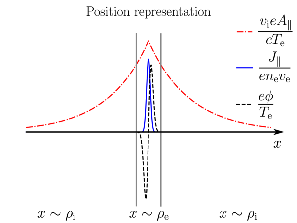
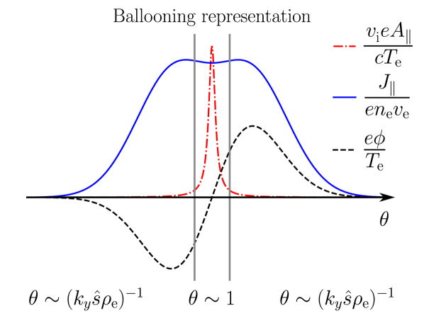
Figure 1: An illustration of a $\beta\ll 1$ micro-tearing instability. We sketch the eigenmodes in two different representations of the radial coordinate. In the position representation, the large-scale macro-tearing stable $A_{\|}$ is driven by an electron current layer at small radial scales close to the rational surface ($x\sim\rho_{\rm{e}}\ll\rho_{\rm{i}}$). In the ballooning representation, $A_{\|}$ is well localised to ballooning angles of $\theta\sim 1$, whereas the current $J_{\|}$ that drives $A_{\|}$ is developed at large ballooning angles $\theta\sim(k_{y}\hat{s}\rho_{\rm{e}})^{-1}\gg 1$. The amplitude of the electrostatic potental $\phi$ is largest in the current layer, with fine radial structures in $x$ and extended tails in $\theta$.

3.1 The inner region – the electron current layer

We first consider the equations for the electron current layer. The derivation proceeds along the same lines as in the electrostatic calculation presented in [32]. We present the results of the calculation in particularly convenient notation for understanding the structure of the model. For completeness, technical details are contained in A.

At large ballooning angles $\theta\sim(k_{y}\hat{s}\rho_{\rm{e}})^{-1}\gg 1$ the gyrokinetic system of equations undergoes several simplifications. First, the nonadiabatic response of ions becomes small, and can be neglected to leading-order. This is due to the large ion gyro orbit compared to the scales of interest, i.e., $k_{r}\rho_{\rm{i}}\gg 1$. Second, two separated scales emerge in the structure of the eigenmodes: the width of the mode in the ballooning space $\theta\sim(k_{y}\hat{s}\rho_{\rm{e}})^{-1}$ becomes much larger than the scale of the periodic geometric variation due to the toroidal geometry $\theta\sim 2\pi\sim 1$. This fact permits a multiscale analysis where we introduce a normalised extended ballooning angle $z=k_{y}\hat{s}|\rho_{\rm{e}}^{\scriptsize\rm{ref}}|\theta\sim 1$ to describe the envelope of the mode, whilst retaining $\theta$ to describe poloidal geometric variation. Here, $\rho_{\rm{e}}^{\scriptsize\rm{ref}}=v_{\rm{e}}/\Omega_{\rm{e}}^{\scriptsize\rm{ref}}$ and $\Omega_{\rm{e}}^{\scriptsize\rm{ref}}=-eB_{\scriptsize{\rm{ref}}}/m_{{\rm{e}}}c$. Third, the leading order balance in the electron gyrokinetic equation becomes one between parallel streaming and radial magnetic drifts. This allows us to determine that the electron nonadiabatic response $h_{{\rm{e}}}$ takes the leading-order form

$$h_{{\rm{e}}}(z,\theta)=H_{\rm{e}}(z)\exp{\left[-{\rm{i}}g_{\rm\scriptscriptstyle N}z\right]},$$ (9)

where $H_{\rm{e}}$ is a smooth function of $z$,

$$g_{\rm\scriptscriptstyle N}(\theta)=\frac{qIw_{\|}}{rB},$$ (10)

and $w_{\|}=v_{\|}/v_{\rm{e}}$. The phase $\exp{\left[-{\rm{i}}g_{\rm\scriptscriptstyle N}z\right]}$ contains all the $\theta$ variation in $h_{{\rm{e}}}$, and is due to the finite width of electron banana orbits in the torus. By going to first order in the asymptotic expansion in $\left(m_{\rm{e}}/m_{\rm{i}}\right)^{1/2}\sim k_{y}|\rho_{\rm{e}}^{\scriptsize\rm{ref}}|$, we can find orbit-averaged equations that describe the envelope of the eigenmode $H_{\rm{e}}$, and thus determine $h_{{\rm{e}}}$ and the fields to leading-order.

The inner region equations for $H_{\rm{e}}$ in the low-$\beta$ ordering (2) are as follows. For passing electrons, we have that

$$\left\langle{w_{\|}g_{\|}}\right\rangle^{\rm{t}}\hat{s}\frac{\partial H_{\rm{e}}}{\partial z}+{\rm{i}}\left(\left\langle{\hat{\omega}_{\rm{M}}}\right\rangle^{\rm{t}}-\hat{\omega}\right)\;H_{\rm{e}}-\hat{\nu}\left\langle{\widehat{C}_{\rm{e}}\left[H_{\rm{e}}\right]}\right\rangle^{\rm{t}}$$

$$=-{\rm{i}}\left(\hat{\omega}_{\ast,{\rm{e}}}-\hat{\omega}\right)F_{0e}\left\langle{\exp{\left[{\rm{i}}g_{\rm\scriptscriptstyle N}z\right]}J_{0}(b_{{\rm{e}}})\frac{e\phi}{T_{\rm{e}}}}\right\rangle^{\rm{t}},$$ (11)

where we have written the equation in a dimensionless fashion. Note that the potential $\phi=\phi(\theta,z)$. Here, $g_{\|}=qR_{0}\bm{b}\cdot\nabla\theta$ with $R_{0}$ a reference major radius,

$$\left\langle{\cdot}\right\rangle^{\rm{t}}=\frac{\int^{\pi}_{-\pi}d\theta\;(\cdot)/w_{\|}g_{\|}}{\int^{\pi}_{-\pi}d\theta/w_{\|}g_{\|}},$$ (12)

is the transit average, and

$$\hat{\omega}_{\rm{M}}=-qR_{0}\frac{d\psi}{dr}\frac{\bm{b}}{B}\times\left(w_{\|}^{2}\bm{b}\cdot\nabla\bm{b}+w_{\perp}^{2}\frac{\nabla B}{2B}\right)\cdot\left(\nabla\alpha+\theta\nabla q\right)-w_{\|}g_{\|}g_{\rm\scriptscriptstyle N}\hat{s}$$ (13)

is a normalised modified magnetic drift frequency, with $w_{\perp}=v_{\perp}/v_{\rm{e}}$. The term $\propto g_{\rm\scriptscriptstyle N}$ in $\hat{\omega}_{\rm{M}}$ arises from the phase in the definition (9) of $H_{\rm{e}}$. The normalised frequency is $\hat{\omega}=qR_{0}\omega/k_{y}|\rho_{\rm{e}}^{\scriptsize\rm{ref}}|v_{\rm{e}}$, and $\hat{\omega}_{\ast,{\rm{e}}}=-(qR_{0}/2L_{n})(1+\eta_{\rm{e}}(\varepsilon/T_{\rm{e}}-3/2))$ is the drive of instability, with $L_{n}=-dr/d\ln n_{\rm{e}}$. The parameter $\hat{\nu}=qR_{0}\nu_{\rm{ee}}/k_{y}|\rho_{\rm{e}}^{\scriptsize\rm{ref}}|v_{\rm{e}}$ is a normalised collision frequency, and

$$\widehat{C}_{\rm{e}}[H_{\rm{e}}]=\frac{1}{\nu_{\rm{ee}}}\left\langle{\exp{\left[{\rm{i}}\left(g_{\rm\scriptscriptstyle N}+g_{\rm\scriptscriptstyle C}\right)z\right]}\mathcal{C}\Big{[}\exp{\left[-{\rm{i}}\left(g_{\rm\scriptscriptstyle N}+g_{\rm\scriptscriptstyle C}\right)z\right]}H_{\rm{e}}\Big{]}}\right\rangle^{\gamma}$$ (14)

is the collision operator, with $\mathcal{C}\left[\cdot\right]$ the drift-kinetic electron collision operator defined in B by equation (45), $\left\langle{\cdot}\right\rangle^{\gamma}$ the gyrophase average at fixed $\varepsilon$ and $\lambda$, $g_{\rm\scriptscriptstyle C}=q(\nabla\psi\cdot\bm{b}\times\bm{w})z/rB$, and $\bm{w}=\bm{v}/v_{\rm{e}}$. The function $b_{{\rm{e}}}$ in equation (11) takes the leading-order value

$$b_{{\rm{e}}}=-q|z\nabla\psi|w_{\perp}/rB.$$ (15)

For trapped electrons, we obtain the bounce-averaged equation

$${\rm{i}}\left(\left\langle{\hat{\omega}_{\rm{M}}}\right\rangle^{\rm{b}}-\hat{\omega}\right)\;H_{\rm{e}}-\hat{\nu}\left\langle{\widehat{C}_{\rm{e}}\left[H_{\rm{e}}\right]}\right\rangle^{\rm{b}}=-{\rm{i}}\left(\hat{\omega}_{\ast,{\rm{e}}}-\hat{\omega}\right)F_{0e}\left\langle{\exp{\left[{\rm{i}}g_{\rm\scriptscriptstyle N}z\right]}J_{0}(b_{{\rm{e}}})\frac{e\phi}{T_{\rm{e}}}}\right\rangle^{\rm{b}},$$ (16)

where the bounce average is defined by

$$\left\langle{\cdot}\right\rangle^{\rm{b}}=\frac{\sum_{\sigma}\int^{\theta^{+}_{b}}_{\theta^{-}_{b}}d\theta\;(\cdot)/|w_{\|}|g_{\|}}{2\int^{\theta^{+}_{b}}_{\theta^{-}_{b}}d\theta/|w_{\|}|g_{\|}},$$ (17)

and $\theta^{\pm}_{b}$ are the upper and lower bounce points in $\theta$, respectively, satisfying $w_{\|}(\theta^{\pm}_{b})=0$. Note the absence of the parallel streaming term in equation (16): trapped particles are unable to pass between magnetic wells, forcing them to remain local in $z$.

Finally, to determine the electrostatic potential $\phi$ that is necessary to solve equations (11) and (16), we have the quasineutrality relation at $k_{r}\rho_{\rm{e}}\sim 1$:

$$\left(\frac{Z_{\rm{i}}T_{\rm{e}}}{T_{\rm{i}}}+1\right)\frac{e\phi}{T_{\rm{e}}}=-\frac{1}{n_{\rm{e}}}\int\exp{\left[-{\rm{i}}g_{\rm\scriptscriptstyle N}z\right]}J_{0}(b_{{\rm{e}}})H_{\rm{e}}\;d^{3}\bm{v},$$ (18)

where we have used that the contribution from the ion nonadiabatic response to quasineutrality is small [32]. Note that even though $H_{\rm{e}}=H_{\rm{e}}(z)$, $\phi=\phi(\theta,z)$ due to the prescence of trapped particles, and due to the $\theta$ dependence of the functions $\exp{\left[-{\rm{i}}g_{\rm\scriptscriptstyle N}z\right]}$ and $J_{0}(b_{{\rm{e}}})$, and the Jacobian of the velocity integral $d^{3}\bm{v}=(2\pi B\varepsilon/m_{{\rm{e}}}^{2}|v_{\|}|)d\varepsilon d\lambda$. The orbit averages in equations (11) and (16) can be calculated explicitly if the potential is expanded in poloidal harmonics, i.e., if we write $\phi(\theta,z)=\sum_{m}\hat{\phi}_{m}(z)\exp{\left[{\rm{i}}m\theta\right]}$.

The parallel vector potential $A_{\|}$ and the perturbation to the magnetic field strength $B_{\|}$ do not appear to leading-order in equations (11) and (16) due to the smallness of $\beta$ assumed by the ordering (2). That the contribution from $B_{\|}$ is small may be verified directly by inspecting equation (6). To see that the contribution from $A_{\|}$ may also be neglected in the $k_{r}\rho_{\rm{e}}\sim 1$ region, we consider a normalised form of Ampère’s law,

$$\frac{\left(k_{\perp}\rho_{\rm{e}}^{\scriptsize\rm{ref}}\right)^{2}}{2\beta_{\rm{e}}}\frac{v_{\rm{e}}}{c}\frac{eA_{\|}}{T_{\rm{e}}}=\frac{J_{\|}}{en_{\rm{e}}v_{\rm{e}}},$$ (19)

with $\beta_{\rm{e}}=8\pi n_{\rm{e}}T_{\rm{e}}/B_{\scriptsize{\rm{ref}}}^{2}\sim\beta$. The current $J_{\|}$ is determined through the definition

$$J_{\|}=-e\int v_{\|}J_{0}(b_{{\rm{e}}})\exp{\left[-{\rm{i}}g_{\rm\scriptscriptstyle N}z\right]}H_{\rm{e}}\;d^{3}\bm{v},$$ (20)

where we have used that the nonadiabatic ion response is small. Since the even and odd in $v_{\|}$ parts of $H_{\rm{e}}$ are mixed by equation (11), the current in the $k_{r}\rho_{\rm{e}}\sim 1$ region must satisfy the ordering

$$\frac{J_{\|}}{en_{\rm{e}}v_{\rm{e}}}\sim\frac{e\phi}{T_{\rm{e}}},$$ (21)

and hence, with the ordering (2), $A_{\|}$ satisfies

$$\frac{v_{\rm{e}}}{c}\frac{eA_{\|}}{T_{\rm{e}}}\sim\beta\frac{e\phi}{T_{\rm{e}}}\sim\left(\frac{m_{\rm{e}}}{m_{\rm{i}}}\right)^{1/2}\frac{e\phi}{T_{\rm{e}}}\ll\frac{e\phi}{T_{\rm{e}}}.$$ (22)

For $\beta\ll 1$, the $k_{r}\rho_{\rm{e}}\sim 1$ inner region is electrostatic to leading order.

3.2 The outer region: determining the matching condition

To solve the gyrokinetic layer equations (11), (16), and (18), we must impose a matching condition at $z=0^{\pm}$ on the incoming distribution of passing particles. This is clear from the cartoon given in figure 1 – in ballooning space we must connect $z<0$ to $z>0$ with an appropriate condition. We now determine the appropriate matching condition in the presence of electromagnetic fluctuations, for the limit $\beta\sim\left(m_{\rm{e}}/m_{\rm{i}}\right)^{1/2}\ll 1$, by considering the physics of the outer region. As the discussion here and in section 3.3 will demonstrate, the $\beta$ ordering (2) is special: $\beta\sim\left(m_{\rm{e}}/m_{\rm{i}}\right)^{1/2}$ is the largest $\beta$ for which the electrons are able to carry a $v_{\rm{e}}$-sized large-scale current; it is also the smallest $\beta$ where $A_{\|}$ is large enough to perturb the electrons from the equilibrium magnetic field line, and hence, introduce electromagnetic physics into the mode.

We begin the calculation by assuming that the passing part of $h_{{\rm{e}}}$, $h^{\rm\scriptstyle passing}_{{\rm{e}}}$, satisfies

$$h^{\rm\scriptstyle passing}_{{\rm{e}}}\sim\frac{e\phi}{T_{\rm{e}}}F_{0e}$$ (23)

in the outer region of the mode, ruling out the appearance of ITG modes and TEMs [32], for which $h^{\rm\scriptstyle passing}_{{\rm{e}}}=\Or\left(\left(m_{\rm{e}}/m_{\rm{i}}\right)^{1/2}e\phi F_{0e}/T_{\rm{e}}\right)$. The natural radial wavenumber scale of the outer region is $k_{r}\rho_{\rm{i}}\sim 1$. This is a consequence of the ordering $k_{y}\rho_{\rm{i}}\sim 1$. Using the orderings (1), (2), and (21), we find that the leading-order electron gyrokinetic equation in this region takes the form

$$v_{\|}\bm{b}\cdot\nabla\theta\frac{\partial h_{{\rm{e}}}}{\partial\theta}={\rm{i}}\left(\omega_{\ast,{\rm{e}}}-\omega\right)\frac{eF_{0e}}{T_{\rm{e}}}\frac{v_{\|}}{c}A_{\|},$$ (24)

where we have ordered

$$\frac{v_{\rm{e}}}{c}\frac{eA_{\|}}{T_{\rm{e}}}\sim\left(\frac{m_{\rm{i}}}{m_{\rm{e}}}\right)^{1/2}\frac{e\phi}{T_{\rm{e}}}.$$ (25)

We justify the ordering (25) by noting that in the outer region the leading-order current satisfies

$$\bm{B}\cdot\nabla\theta\frac{\partial}{\partial\theta}\left(\frac{J_{\|}}{B}\right)=0.$$ (26)

Equation (26) is obtained by first integrating equation (24) over all velocities, and second, by noting that the ion contribution to $J_{\|}$ is dominated by the electron contribution by a factor of $v_{\rm{e}}/v_{\rm{i}}\sim\left({m_{\rm{i}}}/{m_{\rm{e}}}\right)^{1/2}$. Equation (26) states that $J_{\|}/B$ is constant across the outer region: hence, $J_{\|}$ satisfies equation (20) and ordering (21) everywhere. Using this result in equation (19) gives the ordering (25). It is worth noting that an outer solution with constant $J_{\|}/B$ has $A_{\|}\propto B/k_{\perp}^{2}$.

The matching condition for the passing particle distribution function is obtained by integrating equation (24) in $\theta$. We find that the total jump in $h_{{\rm{e}}}$ across the outer region is given by

$$\Delta h_{{\rm{e}}}={\rm{i}}\frac{\left(\omega_{\ast,{\rm{e}}}-\omega\right)}{c}\frac{eF_{0e}}{T_{\rm{e}}}\Delta\Psi,$$ (27)

where

$$\Delta\Psi=\int^{\infty}_{-\infty}\frac{A_{\|}(\theta^{\prime})}{\bm{b}\cdot\nabla\theta^{\prime}}d\theta^{\prime}.$$ (28)

The constant $\Delta\Psi$ measures the net deviation of the perturbed field line from the equilibrium flux surface. If $|\Delta\Psi|>0$, then the mode reconnects field lines. We can see this by considering the flux surface integral $\int^{\pi}_{-\pi}(\cdot)\;d\theta/\bm{B}\cdot\nabla\theta$ of the perturbed magnetic field $\delta\!\bm{B}=-\bm{b}\times\nabla A_{\|}$ in the position representation. We find that the surface-integrated radial magnetic field of a mode at the rational surface is

$$\left.\int^{\pi}_{-\pi}\frac{\delta\!\bm{B}\cdot\nabla r}{\bm{B}\cdot\nabla\theta}\;d\theta\right|_{x=0}=-\frac{k_{y}\Delta\Psi}{B_{\scriptsize{\rm{ref}}}},$$ (29)

where $x$ is the radial position and $x=0$ is the location of the rational surface, and where we have converted the poloidal integral of a fourier sum evaluated at $x=0$ into an integral over the ballooning coordinate.

We can write the matching condition in a convenient form by combining equations (9), and (26)-(28): we use equation (9) to show that $\Delta h_{{\rm{e}}}=\left[H_{\rm{e}}(z)\right]^{z=0^{+}}_{z=0^{-}}$, and we use that $J_{\|}/B$ is a constant across $\theta\sim 1$ to evaluate $\Delta\Psi$ explicitly. In terms of dimensionless variables, we find that the jump that should be imposed on the passing part of the electron distribution function $H_{\rm{e}}$ at $z=0$ is

$$\left[\frac{H_{\rm{e}}(z)}{F_{0e}}\right]^{z=0^{+}}_{z=0^{-}}={\rm{i}}\beta^{\rm eff}\left(\hat{\omega}_{\ast,{\rm{e}}}-\hat{\omega}\right)j_{\|}(0).$$ (30)

Here, we have defined a dimensionless current-like quantity

$$j_{\|}(z)=j^{+}_{\|}(z)-j^{-}_{\|}(z),$$ (31)

with

$$j^{\pm}_{\|}(z)=-\int^{\infty}_{0}\int^{1/B_{\rm max}}_{0}H_{\rm{e}}(z,\varepsilon,\lambda,\sigma=\pm 1)\frac{2\pi\varepsilon B_{\scriptsize{\rm{ref}}}}{n_{\rm{e}}m_{{\rm{e}}}^{2}v_{\rm{e}}}d\lambda d\varepsilon,$$ (32)

and we have defined an effective plasma $\beta$:

$$\beta^{\rm eff}=\beta_{\rm{e}}\frac{2\pi G(\theta_{0})}{\hat{s}k_{y}|\rho_{\rm{e}}^{\scriptsize\rm{ref}}|}.$$ (33)

The parameter $\beta^{\rm eff}$ depends on $(k_{y},\theta_{0})$ and magnetic geometry, through the factors $k_{y}|\rho_{\rm{e}}^{\scriptsize\rm{ref}}|$ and

$$G(\theta_{0})=\frac{\hat{s}}{\pi}\int^{\infty}_{-\infty}\frac{B}{B_{\scriptsize{\rm{ref}}}}\frac{k_{y}^{2}}{k_{\perp}^{2}}\frac{d\theta}{g_{\|}}.$$ (34)

The normalisation of $G(\theta_{0})$ is chosen so that in a magnetic geometry with circular flux surfaces and $\epsilon=r/R\rightarrow 0$, $G(\theta_{0})=1+\Or\left(\epsilon\right)$. In sections 4.2 and 4.3, we use $j^{+}_{\|}$ to visualise $H_{\rm{e}}$ for forward-going particles. The matching condition (30) leads us to expect a discontinuity in $j^{+}_{\|}(z)$ at $z=0$. Nonetheless, $j_{\|}$, which is $\propto J_{\|}/B$ for $z\ll 1$, is continuous across $z=0$ due to the fact that the jump in $H_{\rm{e}}$ is even in $v_{\|}$.

In the calculation presented above, it might seem that we have neglected to consider the impact of the electron inertial scale $\delta_{\rm{e}}$ that is intermediate to $\rho_{\rm{e}}$ and $\rho_{\rm{i}}$: $\rho_{\rm{e}}\ll\delta_{\rm{e}}\ll\rho_{\rm{i}}$. The scale of $k_{r}\delta_{\rm{e}}\sim 1$ is often singled out as interesting because of the characterising property that (by equations (21) and (19)) $v_{\rm{e}}A_{\|}/c\sim\phi$ and so both fields enter simultaneously into the source of the electron gyrokinetic equation. In C, we prove that, in the orderings (1) and (2) considered here, the leading order distribution function envelope $H_{\rm{e}}$ is constant across the $k_{r}\delta_{\rm{e}}\sim 1$ region. This means that fluctuations at the scale of $k_{r}\delta_{\rm{e}}\sim 1$ do not modify the matching condition (30).

Note that the current appearing in equation (30) is evaluated purely from $H_{\rm{e}}$. If the microinstability is unstable to leading-order, then the microinstability is independent of the ion nonadiabatic response to leading-order. If the microinstability happens to be stable at leading order, then the nonadiabatic ion response must be included in the calculation to find a $\left(m_{\rm{e}}/m_{\rm{i}}\right)^{1/2}$ small growth (or damping) rate.

Finally, we comment that the $\beta\ll 1$ ballooning-space calculation presented above is related to the usual position-space $\beta\ll 1$ matching for tearing modes at large toroidal mode number. In position space, described by the radial coordinate $x$ measuring position from the rational surface, taking $\beta\ll 1$ gives $A_{\|}\propto\exp{\left[-k_{y}|x|\right]}$ in the outer region ($x\sim\rho_{\rm{i}}$) with $A_{\|}(x)$ a constant in the inner region where $x\sim\rho_{\rm{e}}$. The matching is carried out by ensuring $\Delta^{\prime}=d\ln A_{\|}(x)/dx$ is the same at the boundary of the inner and outer regions. In ballooning space, we have shown above that taking $\beta\ll 1$ gives $J_{\|}/B$ a constant in the outer region ($\theta\sim 1$), with $A_{\|}(\theta)\propto B/k_{\perp}^{2}$. As a result, the inner region ($z=k_{y}\hat{s}|\rho_{\rm{e}}^{\scriptsize\rm{ref}}|\theta\sim 1$) observes a constant $\Delta\Psi$ in the jump in electron distribution function $h_{{\rm{e}}}$ across the outer region, cf. equation (27). In the ballooning space representation, the constant $\Delta\Psi$ forces fluctuations in the inner region just as a constant $A_{\|}(x=0)$ forces the inner region fluctuations in the position space representation. Note that in a sheared slab the ballooning-space outer solution $1/k_{\perp}^{2}=k_{y}^{-2}(1+\hat{s}^{2}(\theta-\theta_{0})^{2})^{-1}$ is proportional to the fourier transform of the position-space outer solution $\exp{\left[-k_{y}|x|\right]}$ – demonstrating that the “constant-$A_{\|}$” and “constant-$\Delta\Psi$” approximations are equivalent, cf. [12].

3.3 Subsidiary limits

The electrostatic limit of the matching condition (30) is simple. If we take $\beta^{\rm eff}$ to be small ($\beta_{\rm{e}}\ll k_{y}|\rho_{\rm{e}}^{\scriptsize\rm{ref}}|$) then (30) takes the leading-order form

$$\left[\frac{H_{\rm{e}}(z)}{F_{0e}}\right]^{z=0^{+}}_{z=0^{-}}=0,$$ (35)

which is the matching condition for electrostatic, electron-driven instabilities localised to the mode-rational surface [32]. Note that the matching condition (35) is independent of $\theta_{0}$, and hence, in the electrostatic limit the leading-order mode frequency and growth rate are independent of $\theta_{0}$ [32].

It is also interesting to consider the subsidiary limit $\beta^{\rm eff}\gg 1$ ($\beta_{\rm{e}}\gg k_{y}|\rho_{\rm{e}}^{\scriptsize\rm{ref}}|$). For this limit, it is instructive to write the matching condition in the form

$$\left[\frac{H_{\rm{e}}(z)}{F_{0e}}\right]^{z=0^{+}}_{z=0^{-}}={\rm{i}}\left(\hat{\omega}_{\ast,{\rm{e}}}-\hat{\omega}\right)\Delta\widehat{\Psi},$$ (36)

where

$$\Delta\widehat{\Psi}=\frac{v_{\rm{e}}k_{y}|\rho_{\rm{e}}^{\scriptsize\rm{ref}}|}{qR_{0}c}\frac{e\Delta\Psi}{T_{\rm{e}}}=\beta^{\rm eff}j_{\|}(0).$$ (37)

It is clear from equation (36) that taking $\beta^{\rm eff}\gg 1$ cannot change the relationship between the sizes of $H_{\rm{e}}$ and $\Delta\widehat{\Psi}$. This is also apparent in equation (24): electron parallel streaming must always balance the magnetic field line perturbations from $A_{\|}$, once $A_{\|}$ is sufficiently large, and so the ordering (25) must remain satisfied. Instead of making $\Delta\widehat{\Psi}$ large, taking $\beta^{\rm eff}\gg 1$ results in a constraint on the current produced by the layer. To preserve the ordering $H_{\rm{e}}/F_{0e}\sim\Delta\widehat{\Psi}\sim e\phi/T_{\rm{e}}$ as $\beta^{\rm eff}\rightarrow\infty$, we must have that

$$j_{\|}(0)=\Or\left(\frac{1}{\beta^{\rm eff}}\frac{e\phi}{T_{\rm{e}}}\right).$$ (38)

Solving the model equations in this limit requires us to regard $\Delta\widehat{\Psi}$ as a free parameter in (36). We fix $\Delta\widehat{\Psi}$ relative to $e\phi/T_{\rm{e}}$ by finding the value of $\Delta\widehat{\Psi}$ that makes equation (38) satisfied, whilst simultaneously finding $\hat{\omega}$ such that equations (11), (16), (18), and (36) are satisfied. Note that the parameter $\beta^{\rm eff}$ disappears from the leading-order eigenvalue problem when $\beta^{\rm eff}\gg 1$. This means that the frequency $\hat{\omega}$ and eigenmodes become independent of $\beta^{\rm eff}$ once $\beta^{\rm eff}$ is sufficiently large.

The constraint (38) appears in sheared-slab models as the requirement that large-scale electron currents cannot leak out of the rational-surface layer. In the extreme case that $\beta_{\rm{e}}$ becomes of order unity, then $\beta^{\rm eff}\sim\left({m_{\rm{i}}}/{m_{\rm{e}}}\right)^{1/2}$ and equation (38) suggests that the large-scale current produced by the electron layer $J_{\|}\sim en_{\rm{e}}v_{\rm{i}}(e\phi/T_{\rm{e}})$. This current is comparable to the current carried by the ions in the outer region, breaking the assumption that the ion current can be neglected in the calculation of $J_{\|}$. Separate papers will consider this $\beta_{\rm{e}}\sim 1$ limit, and resolve this issue.

3.4 Scaling predictions

A significant prediction made by the theory is that the leading-order dispersion relation should depend on physics parameters in a precise manner. By inspecting the form of the model equations (11), (16), (18), and (30), we observe that

$$\omega=\frac{v_{\rm{e}}}{qR_{0}}k_{y}|\rho_{\rm{e}}^{\scriptsize\rm{ref}}|\;\hat{\omega}\left(\beta^{\rm eff},\hat{\nu},a/L_{n},a/L_{T_{\rm{e}}},\tau,Z_{\rm{i}},\bm{g}\right),$$ (39)

where we have indicated that $\hat{\omega}$ is a function of physics parameters, with $\tau=T_{\rm{i}}/Z_{\rm{i}}T_{\rm{e}}$ and $\bm{g}$ a vector of geometrical parameters that are needed to describe the local flux surface. Note that a dispersion relation of the form (39) implies that $\omega$ depends on $k_{y}$ only through the overall linear pre-factor, $\beta^{\rm eff}$, and $\hat{\nu}$. The definition of $\beta^{\rm eff}$, equation (33), also provides an interesting explanation for why electron-driven electromagnetic modes tend to be observed at the longest wavelengths: $\beta^{\rm eff}$ is larger for smaller $k_{y}|\rho_{\rm{e}}^{\scriptsize\rm{ref}}|$. We might expect that below a certain critical $\beta^{\rm eff}$ the electromagnetic microinstabilities are stable, and hence, there is likely to be a maximum $k_{y}$ for instability. In the limit $\beta^{\rm eff}\gg 1$, the model predicts that $\hat{\omega}$ tends to a constant, and hence we expect that $\omega$ goes linearly with $k_{y}|\rho_{\rm{e}}^{\scriptsize\rm{ref}}|$ for the very smallest $k_{y}$. Whether or not there is a stronger cut-off at small $k_{y}|\rho_{\rm{e}}^{\scriptsize\rm{ref}}|$ ($\beta^{\rm eff}\gg 1$) can only be determined by a theory that handles a $\beta\sim 1$ ordering.

The collisionality dependence of $\hat{\omega}$ through the parameter $\hat{\nu}=qR_{0}\nu_{\rm{ee}}/k_{y}|\rho_{\rm{e}}^{\scriptsize\rm{ref}}|v_{\rm{e}}$ states that for a fixed collision frequency $\nu_{\rm{ee}}$, modes of smaller $k_{y}|\rho_{\rm{e}}^{\scriptsize\rm{ref}}|$ are more collisional. Taking $\hat{\nu}\rightarrow\infty$ in the model equations (11), (16) and (18) yields the semicollisional limit [32], whereas taking $\hat{\nu}\rightarrow 0$ yields the collisionless limit. Hence, depending on the value of $qR\nu_{\rm{ee}}/v_{\rm{e}}$, the $k_{y}$ spectrum of a $k_{y}|\rho_{\rm{e}}^{\scriptsize\rm{ref}}|\ll 1$ MTM potentially spans modes in the semicollisional limit $\hat{\nu}\gg 1$ at very low $k_{y}|\rho_{\rm{e}}^{\scriptsize\rm{ref}}|$, to modes in the collisionless limit ($\hat{\nu}\ll 1$) at more moderate $k_{y}|\rho_{\rm{e}}^{\scriptsize\rm{ref}}|$.

4 Numerical evidence for the $\beta_{\rm{e}}\sim\left(m_{\rm{e}}/m_{\rm{i}}\right)^{1/2}$ theory

Finding a general analytical solution of the model equations (11), (16), (18), and (30) is challenging. A numerical implementation is likely to be necessary to solve the model in magnetic geometries of interest. To test the analytical theory, we compare the intrinsic scalings predicted by the theory to numerical results using the $\delta\!f$ gyrokinetic code GS2 [34]. We choose to examine microinstabilities in an experimentally relevant local equilibrium taken from close to mid-radius in a MAST H-mode plasma (MAST discharge #6252). This discharge was examined previously using gyrokinetic simulations [10], demonstrating the qualitative behaviour of MTMs in MAST by performing scans in $\nu_{\rm{ee}}$, $a/L_{T_{\rm{e}}}$, $\beta$ and $k_{y}$. We note that the scans in $\nu_{\rm{ee}}$ (at a fixed $k_{y}$) showed that for $\nu_{\rm{ee}}$ too large or small, the MTM is stabilised. Similar behaviour has been observed in other discharges [35, 14].

We examine fastest-growing eigenmodes using GS2 as an initial value solver, including kinetic ions, kinetic electrons and all three fields $\phi$, $A_{\|}$, and $B_{\|}$. For simplicity, we consider a two-species plasma consisting of ions and electrons, with $Z_{\rm{i}}=1$ and $T_{\rm{i}}=T_{\rm{e}}$. We specify the magnetic geometry using the local Miller parameterisation [36], through the following GS2  input parameters: the reference major radius $R_{0}=(R_{\rm max}+R_{\rm min})/2$ with $R_{\rm max}$ and $R_{\rm min}$ the maximum and minimum major radial positions on the flux surface, respectively; the minor radius $r$ of the flux surface of interest; the safety factor $q$; the magnetic shear $\hat{s}=(q/r)dq/dr$; $\beta_{\rm{e}}=8\pi n_{\rm{e}}T_{\rm{e}}/B_{\scriptsize{\rm{ref}}}^{2}$, with $B_{\scriptsize{\rm{ref}}}=I/R_{\rm geo}$; the normalised pressure gradient $\beta^{\prime}=(8\pi/B_{\scriptsize{\rm{ref}}}^{2})dp/d\rho$, with $p$ the total equilibrium pressure, $\rho=r/a$, and the normalising length $a$ the half-diameter of the last closed flux surface; the Shafranov shift derivative $dR_{0}/dr$; the elongation $\kappa$; the elongation derivative $\kappa^{\prime}=d\kappa/d\rho$; the triangularity $\delta$; and the triangularity derivative $\delta^{\prime}=d\delta/d\rho$. The equilibrium profiles are set by the normalised gradients $a/L_{T_{s}}=-d\ln T_{s}/d\rho$ and $a/L_{n}=-d\ln n_{s}/d\rho$. We treat the collision frequencies $\nu_{\rm{ee}}=\nu_{\rm{ei}}/Z_{\rm{i}}$ and $\nu_{\rm{ii}}$ as independent input parameters, defined according to the GS2  convention [37]

$$\nu_{ss^{\prime}}=\frac{\sqrt{2}\pi n_{s^{\prime}}Z_{s}^{2}Z_{s^{\prime}}^{2}e^{4}\ln\Lambda}{m_{s}^{1/2}T_{s}^{3/2}}.$$ (40)

The Coloumb logarithm $\ln\Lambda$ in equation (40) has the physical value $\ln\Lambda\approx 17$ [38]. The local equilibrium parameters for MAST discharge #6252 are provided in Table 1. The choice of $R_{\rm geo}$ corresponds to choosing $B_{\scriptsize{\rm{ref}}}=0.458{\rm{T}}$, the toroidal magnetic field on the magnetic axis in the MAST discharge [10]. The numerical resolutions are described in D.

$R_{0}/a$	1.57	$R_{\rm geo}/a$	1.46
$r/a$	0.552	$\beta^{\prime}$	-0.248
$q$	1.34	$\beta_{\rm{e}}$	0.0494
$\hat{s}$	0.538	$a/L_{T_{\rm{e}}}$	2.70
$dR_{0}/dr$	-0.146	$a/L_{n}$	-0.230
$\kappa$	1.47	$a/L_{T_{\rm{i}}}$	2.70
$\kappa^{\prime}$	0.0512	$a\nu_{\rm{ee}}/v_{\rm{i}}$	0.303
$\delta$	0.162	$a\nu_{\rm{ii}}/v_{\rm{i}}$	0.00884
$\delta^{\prime}$	0.333	$Z_{\rm eff}$	1.0

Table 1: Local equilibrium and Miller geometry parameters used to study micro-stability in MAST discharge #6252. Previous micro-stability studies of this discharge utilised a numerical equilibrium, cf. [10]. The parameters are defined in the main text.

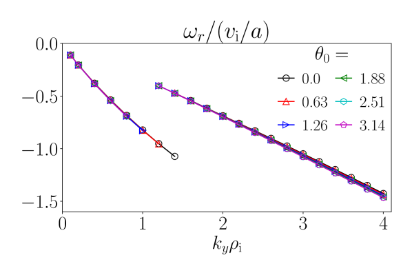
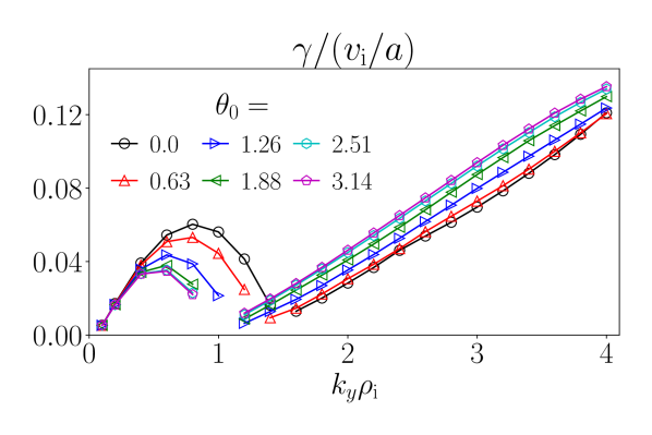
Figure 2: The real frequency $\omega_{{\rm{r}}}$ (left) and growth rate $\gamma$ (right) as a function of $(k_{y}\rho_{\rm{i}},\theta_{0})$ in the MAST discharge #6252, for the physical mass ratio $\left({m_{\rm{i}}}/{m_{\rm{e}}}\right)^{1/2}=61$. The modes to the left of the discontinuity in $\omega_{{\rm{r}}}$ are the MTMs identified in [10], whereas the modes to the right of the discontinuity are electrostatic, electron-driven modes with extended tails; see, e.g., [31, 32].

4.1 The wavenumber spectrum

We first calculate the fastest-growing microinstabilities as a function of $(k_{y}\rho_{\rm{i}},\theta_{0})$, for the equilibrium parameters provided in table 1, and the physical Deuterium-ion-to-electron mass ratio $\sqrt{m_{{\rm D}}/m_{{\rm{e}}}}=61$. The real frequency $\omega_{{\rm{r}}}$ and growth rate $\gamma$ are plotted in figure 2. The discontinuity in $\omega_{{\rm{r}}}$ indicates a transition between different mode branches: to the left of the discontinuity, we find the MTMs that were previously reported by Applegate et al. [10]; and to the right of the discontinuity, we find electrostatic, electron-driven modes with extended tails in ballooning angle. The presence of the electrostatic modes was not reported in [10], where only tearing-parity modes at $\theta_{0}=0$ were considered. We show typical eigenmodes in figure 3: we consider a MTM at $(k_{y}\rho_{\rm{i}},\theta_{0})=(0.8,0.0)$ and an electrostatic mode at $(k_{y}\rho_{\rm{i}},\theta_{0})=(2.2,0.0)$. Note that both instabilities have potentials $\phi$ with an extended structure in $\theta$. The electrostatic mode has small contributions from $A_{\|}$ and $B_{\|}$, and carries little current. The MTM has features that match the expectations given by the theory for electromagnetic modes (cf. figure 1). The potential $\phi$ and $J_{\|}$ are extended, $A_{\|}$ is significant only for $\theta\sim 1$, and $B_{\|}$ can be neglected because it is small everywhere. The normalisations suggest that the orderings in section 3 are valid. We now provide a more precise test of the theory.

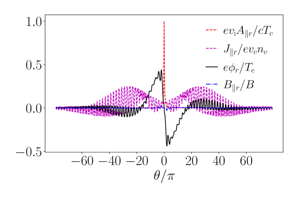
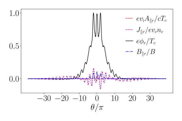
Figure 3: Eigenmodes from the wavenumber spectrum shown in figure 2. We consider the MTM at $(k_{y}\rho_{\rm{i}},\theta_{0})=(0.8,0.0)$ (left) and the electrostatic mode at $(k_{y}\rho_{\rm{i}},\theta_{0})=(2.2,0.0)$ (right). For the MTM, we normalise the fields with the value of $ev_{\rm{i}}A_{\|}/cT_{\rm{e}}$ at the $\theta$ location where $|A_{\|}|$ is maximum. For the electrostatic mode, we normalise the fields with the value of $e\phi/T_{\rm{e}}$ at the $\theta$ location where $|\phi|$ is maximum. We plot only the real parts of the eigenmodes, noting that the imaginary parts have similar sizes. Note that $B_{\|}$ is small for both modes, and that $J_{\|}$ and $A_{\|}$ are only significant in the MTM.

4.2 Testing the $\left(m_{\rm{e}}/m_{\rm{i}}\right)^{1/2}$ scalings: the MTM

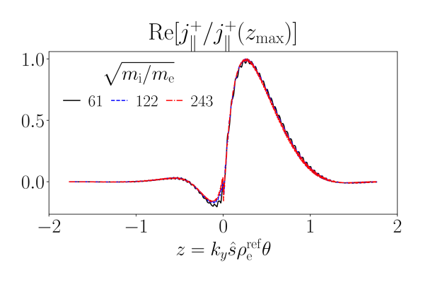
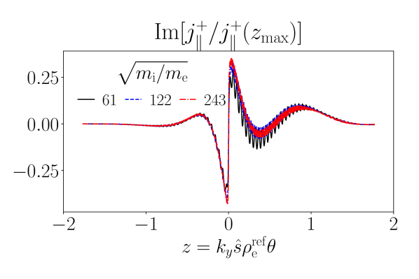
Figure 4: The current-like quantity $j^{+}_{\|}$, defined by equation (32), for the MTM at $(k_{y}\rho_{\rm{i}},\theta_{0})=(0.8,0.0)$. The quantity $j^{+}_{\|}$ is a measure of the forward-going electron distribution function $H_{\rm{e}}$ that is defined by equation (9). Note the smoothness of $j^{+}_{\|}$ for $|z|\sim 1$, and the discontinuity at $z\approx 0$.

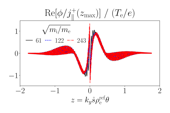
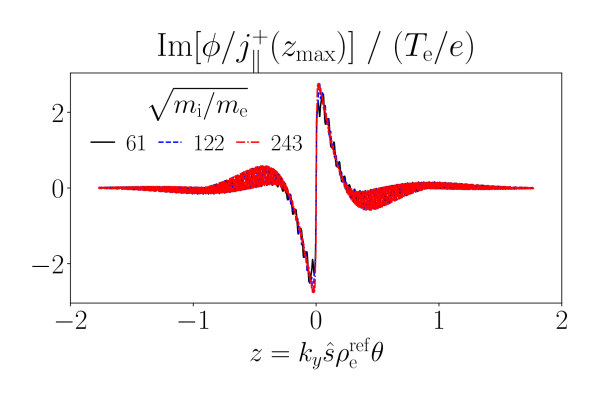
Figure 5: The real and imaginary parts of the electrostatic potential $\phi$ for the MTM at $(k_{y}\rho_{\rm{i}},\theta_{0})=(0.8,0.0)$. The potential is normalised by $j^{+}_{\|}$ where $|j^{+}_{\|}(z)|$ is maximum. That the curves overlay for different $\left({m_{\rm{i}}}/{m_{\rm{e}}}\right)^{1/2}$ indicates that the ordering (23) is satisfied, and that the width of the mode obeys $z=k_{y}\hat{s}\rho_{\rm{e}}^{\scriptsize\rm{ref}}\theta\sim 1$.

We can demonstrate that both the MTMs and the electrostatic, electron-driven modes shown in figure 3 satisfy the correct scalings to be described by the analytical theory. To test the scalings, we perform linear simulations at fixed $k_{y}\rho_{\rm{i}}$ for varying $\left({m_{\rm{i}}}/{m_{\rm{e}}}\right)^{1/2}$. Crucially, when we double $\left({m_{\rm{i}}}/{m_{\rm{e}}}\right)^{1/2}$ we halve $\beta_{\rm{e}}$ so that the ordering (2) remains satisfied. This means that we scale $\beta_{\rm{e}}\propto\left(m_{\rm{e}}/m_{\rm{i}}\right)^{1/2}$ so that $\beta_{\rm{e}}/k_{y}\rho_{\rm{e}}\sim\beta^{\rm eff}$ is held fixed at a given $k_{y}\rho_{\rm{i}}$. We hold $a\nu_{\rm{ee}}/v_{\rm{i}}$ fixed in the scan, consistent with the ordering (1), and we hold fixed the other geometrical parameters in table 1, including $\beta^{\prime}$. We plot the eigenmodes as a function of the expansion parameter $\left({m_{\rm{i}}}/{m_{\rm{e}}}\right)^{1/2}$, and demonstrate that the width of the eigenmode scales like $k_{y}\hat{s}\rho_{\rm{e}}^{\scriptsize\rm{ref}}\theta\sim 1$, and that the orderings for the fields are satisfied.

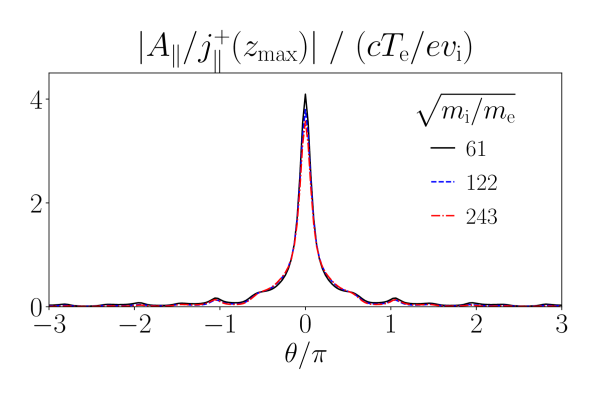
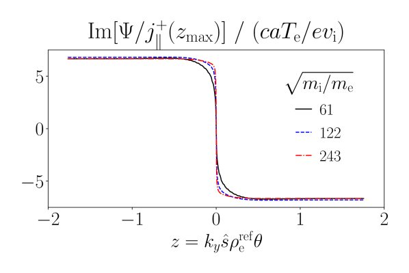
Figure 6: Plots of the parallel vector potential $A_{\|}$ and the auxiliary field $\Psi$ (defined by equation (41)), for the MTM at $(k_{y}\rho_{\rm{i}},\theta_{0})=(0.8,0.0)$. We normalise the eigenmodes by $j^{+}_{\|}$ where $|j^{+}_{\|}(z)|$ is maximum, cf. figure 4. Note that $A_{\|}$ is well localised to $\theta\sim 1$ as $\left(m_{\rm{e}}/m_{\rm{i}}\right)^{1/2}\rightarrow 0$, and that the ordering (25) is satisfied. The field $\Psi$ resembles a Heavyside function as $\left(m_{\rm{e}}/m_{\rm{i}}\right)^{1/2}\rightarrow 0$, consistent with the asymptotic theory, where the jump $\Delta\Psi$ is entirely due to the $A_{\|}$ at $\theta\sim 1$, cf equation (28). The curves of $\Psi$ overlay for $z\sim 1$, consistent with the ordering (25) and the matching condition (27).

We first consider the MTM at $(k_{y}\rho_{\rm{i}},\theta_{0})=(0.8,0.0)$. In figure 4, we visualise the forward-going part of the electron distribution function $H_{\rm{e}}$ using the real and imaginary parts of the current-like quantity $j^{+}_{\|}$ (defined by equation (32), where $H_{\rm{e}}$ is calculated from the GS2 $h_{{\rm{e}}}$ eigenmode via equation (9)). We note that $j^{+}_{\|}$ is a smooth function of $z$ for $|z|\sim 1$, verifying a key element of the theory, equation (9). We also note that there is a discontinuity near $z=0$ – this is consistent with the matching condition (30). We must choose an appropriate normalisation for the eigenmodes of $\phi$ and $A_{\|}$: we select $j^{+}_{\|}(z_{{\rm max}})$, the value of $j^{+}_{\|}(z)$ at the maximum value of $|j^{+}_{\|}(z)|$. In figure 5, we plot the real and imaginary parts of $\phi$. The eigenmodes show oscillatory behaviour due to the $2\pi$ periodic variation of the magnetic geometry. The envelope of the eigenmodes overlay well, confirming that the electron nonadiabatic response sources the leading component of $\phi$, consistent with ordering (23) and equation (18). Finally, in figure 6, we plot $A_{\|}$ in the region $\theta\sim 1$, and the auxiliary field

$$\Psi(\theta)=\int^{\theta}_{-\infty}\frac{A_{\|}(\theta^{\prime})}{\bm{b}\cdot\nabla\theta^{\prime}}d\theta^{\prime}-\frac{1}{2}\int^{\infty}_{-\infty}\frac{A_{\|}(\theta^{\prime})}{\bm{b}\cdot\nabla\theta^{\prime}}d\theta^{\prime}.$$ (41)

Note that $\Delta\Psi=\Psi(\infty)-\Psi(-\infty)$. We see that $A_{\|}$ is well localised to $\theta\sim 1$, the ordering (25) is satisfied, and that the variation in $\Psi$ is increasingly localised to $z\approx 0$ as $\left(m_{\rm{e}}/m_{\rm{i}}\right)^{1/2}\rightarrow 0$, consistent with a constant $\Delta\Psi$ observed by the inner region in the matching.

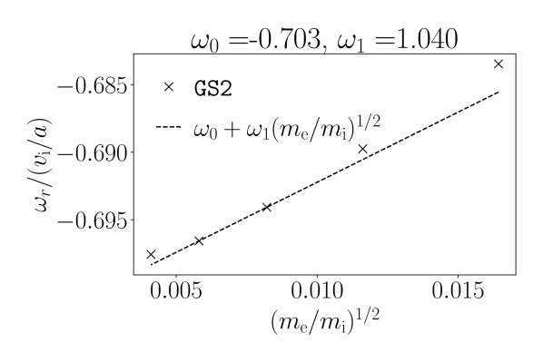
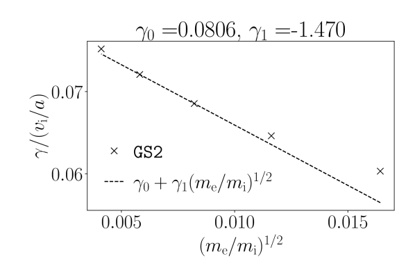
Figure 7: The real frequency $\omega_{{\rm{r}}}$ and growth rate $\gamma$ of the MTM at $(k_{y}\rho_{\rm{i}},\theta_{0})=(0.8,0.0)$ as a function of the expansion parameter $\left(m_{\rm{e}}/m_{\rm{i}}\right)^{1/2}$. Linear fits are provided to show that the variation in $\omega_{{\rm{r}}}$ and $\gamma$ are consistent with the $\left(m_{\rm{e}}/m_{\rm{i}}\right)^{1/2}$ expansion: the fit coefficients are of order unity. The growth rate increases for reducing $\left(m_{\rm{e}}/m_{\rm{i}}\right)^{1/2}$, possibly consistent with calculations of the impact of higher-order corrections from ions on tearing modes [20].

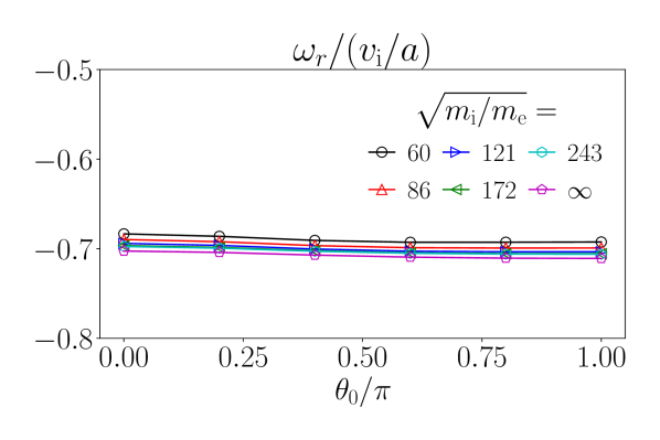
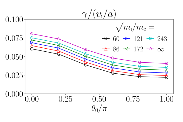
Figure 8: The real frequency $\omega_{{\rm{r}}}$ and growth rate $\gamma$ of the MTMs at $k_{y}\rho_{\rm{i}}=0.8$ as a function of $\theta_{0}$ and the expansion parameter $\left({m_{\rm{i}}}/{m_{\rm{e}}}\right)^{1/2}$. The points in the curve labelled by $\left({m_{\rm{i}}}/{m_{\rm{e}}}\right)^{1/2}=\infty$ are computed from linear fits, see figure 7. In section 5, we show that the variation of $\gamma$ with $\theta_{0}$ is explained by the $\theta_{0}$ dependence of $\beta^{\rm eff}$.

In addition to considering the eigenmodes, it is important to observe the impact of varying $\left(m_{\rm{e}}/m_{\rm{i}}\right)^{1/2}$ on the complex frequency $\omega=\omega_{{\rm{r}}}+{\rm{i}}\gamma$. We should anticipate a leading order component of $\omega$ that is independent of $\left(m_{\rm{e}}/m_{\rm{i}}\right)^{1/2}$, described by the leading-order asymptotic theory, and a correction that is small in $\left(m_{\rm{e}}/m_{\rm{i}}\right)^{1/2}$. In figure 7, we plot the real frequency $\omega_{{\rm{r}}}$ and the growth rate $\gamma$ as a function of $\left(m_{\rm{e}}/m_{\rm{i}}\right)^{1/2}$. We provide linear fits to indicate size of the variation with $\left(m_{\rm{e}}/m_{\rm{i}}\right)^{1/2}$. Although the leading-order growth rate $\gamma_{0}$ is numerically small compared to $\omega_{0}$, the fit coefficients are of order unity, consistent with the theory. We note that $\gamma$ increases as $\left(m_{\rm{e}}/m_{\rm{i}}\right)^{1/2}\rightarrow 0$, which would indicate that the $\left(m_{\rm{e}}/m_{\rm{i}}\right)^{1/2}$ small corrections to $\gamma_{0}$ are stabilising. Although we have not computed these higher-order corrections here, we note that this result is consistent with the calculation for the higher-order impact of ions on tearing modes in sheared-slab geometry, see [20]. Finally, in figure 8, we plot $\omega_{{\rm{r}}}$ and $\gamma$ as a function of $\theta_{0}$ at fixed $k_{y}\rho_{\rm{i}}=0.8$. We observe that $\gamma$ has variation with $\theta_{0}$ even as $\left(m_{\rm{e}}/m_{\rm{i}}\right)^{1/2}\rightarrow 0$. In section 5, we prove that this variation in $\theta_{0}$ is explained by the $\theta_{0}$ dependence of $\beta^{\rm eff}$ through the geometrical factor $G(\theta_{0})$.

4.3 Testing the $\left(m_{\rm{e}}/m_{\rm{i}}\right)^{1/2}$ scalings: the electrostatic mode

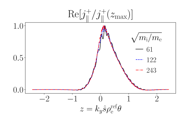
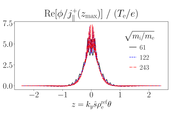
Figure 9: The real parts of the current-like function $j^{+}_{\|}$ and the electrostatic potential $\phi$ for the electrostatic mode at $(k_{y}\rho_{\rm{i}},\theta_{0})=(2.2,0.0)$. We normalise the eigenmode by $j^{+}_{\|}$ where $|j^{+}_{\|}(z)|$ is maximum. The field $j^{+}_{\|}$ is a measure of the forward-going electron distribution function. The fact that the curves overlay indicates that the ordering (23) is satisfied, and that the width of the mode satisfies $k_{y}\hat{s}\rho_{\rm{e}}^{\scriptsize\rm{ref}}\theta\sim 1$.

We perform the same $\left(m_{\rm{e}}/m_{\rm{i}}\right)^{1/2}\rightarrow 0$ analysis for the predominantly electrostatic mode at $(k_{y}\rho_{\rm{i}},\theta_{0})=(2.2,0.0)$. In figure 9, we plot the real parts of the current-like field $j^{+}_{\|}$, and the potential $\phi$. The imaginary parts have a similar order of magnitude and structure. Figure 9 reveals that the mode is an electron-driven, electrostatic mode with large tails, like those observed in [32]. Because the envelopes of the eigenmodes overlay well for different $\left({m_{\rm{i}}}/{m_{\rm{e}}}\right)^{1/2}$, we conclude that the width of the mode satisfies $z=k_{y}\hat{s}\rho_{\rm{e}}^{\scriptsize\rm{ref}}\theta\sim 1$, and the ordering (23) is satisfied.

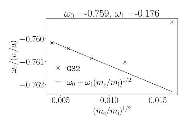
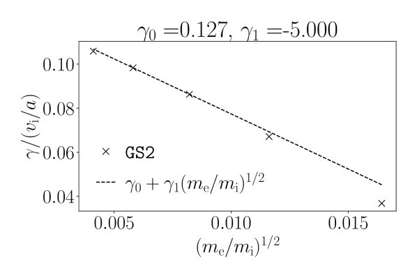
Figure 10: The growth rate $\gamma$ and real frequency $\omega_{{\rm{r}}}$ of the electrostatic mode at $(k_{y}\rho_{\rm{i}},\theta_{0})=(2.2,0.0)$, plotted for different values of the expansion parameter $\left(m_{\rm{e}}/m_{\rm{i}}\right)^{1/2}$. We would expect that for small $\left(m_{\rm{e}}/m_{\rm{i}}\right)^{1/2}$, $\gamma$ and $\omega_{{\rm{r}}}$ should be well represented by a constant plus a linear function of $\left(m_{\rm{e}}/m_{\rm{i}}\right)^{1/2}$: linear fits are provided to indicate the order of the variation with $\left(m_{\rm{e}}/m_{\rm{i}}\right)^{1/2}$. The values of $\omega_{0}$, $\omega_{1}$, $\gamma_{0}$, and $\gamma_{1}$ can be considered to be of order unity, although $\gamma_{0}$ is surprisingly small, and $\gamma_{1}$ is surprisingly large. Even though a nonasymptotic trend is observed in $\omega_{{\rm{r}}}$ for the larger values of $\left(m_{\rm{e}}/m_{\rm{i}}\right)^{1/2}$, the overall variation in $\omega_{{\rm{r}}}$ is small.

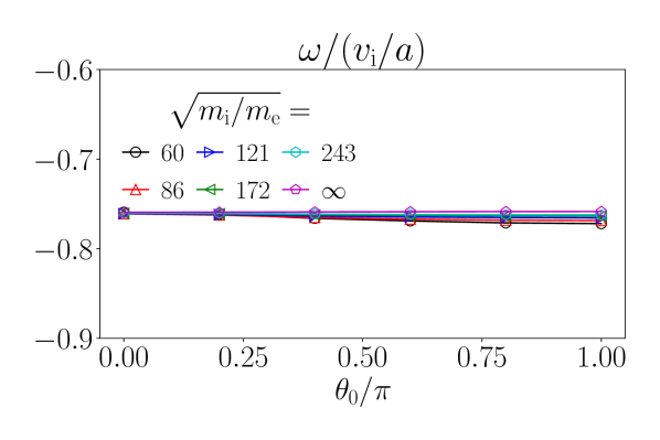
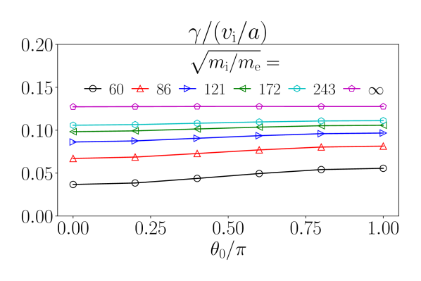
Figure 11: The real frequency $\omega_{{\rm{r}}}$ and growth rate $\gamma$ of the electrostatic modes at $k_{y}\rho_{\rm{i}}=2.2$, as a function of $\theta_{0}$, plotted for different values of the expansion parameter $\left({m_{\rm{i}}}/{m_{\rm{e}}}\right)^{1/2}$. The points in the curve labelled by $\left({m_{\rm{i}}}/{m_{\rm{e}}}\right)^{1/2}=\infty$ are computed from linear fits, see figure 10. Note that as $\left(m_{\rm{e}}/m_{\rm{i}}\right)^{1/2}\rightarrow 0$, $\gamma$ and $\omega_{{\rm{r}}}$ tend to constants that are independent of $\theta_{0}$, consistent with the leading-order electrostatic theory [32].

In figure 10, we plot the real frequency and growth rate of the mode as a function of $\left(m_{\rm{e}}/m_{\rm{i}}\right)^{1/2}$. This reveals that $\omega_{{\rm{r}}}$ is well converged for the physical $\left(m_{\rm{e}}/m_{\rm{i}}\right)^{1/2}=1/61$: $\omega_{{\rm{r}}}$ changes only in the third decimal place. However, $\gamma$ has a surprisingly large linear variation with $\left(m_{\rm{e}}/m_{\rm{i}}\right)^{1/2}$, meaning that $\gamma_{0}$ differs noticeably from $\gamma$ for $\left(m_{\rm{e}}/m_{\rm{i}}\right)^{1/2}=1/61$. This result may be caused by the fact that the mode is sufficiently close to marginal stability for first-order corrections to matter. We note that the fact that the mode is more unstable for smaller $\left(m_{\rm{e}}/m_{\rm{i}}\right)^{1/2}$ (as in the MTM case, cf. figure 7) suggests that the leading-order model of section 3 might provide a conservative upper bound on any linear growth rate. We examine the $\theta_{0}$ dependence of $\omega$ in figure 11. The real frequency $\omega_{{\rm{r}}}$ is a constant in $\theta_{0}$, consistent with the electrostatic limit described in section 3.3 [32]. The growth rate varies with $\theta_{0}$ for the physical mass ratio $\left({m_{\rm{i}}}/{m_{\rm{e}}}\right)^{1/2}=61$, but increasing $\left({m_{\rm{i}}}/{m_{\rm{e}}}\right)^{1/2}$ causes $\gamma$ to tend to a constant that is independent of $\theta_{0}$, consistent with the leading-order theory.

5 Testing the effective $\beta_{\rm{e}}$

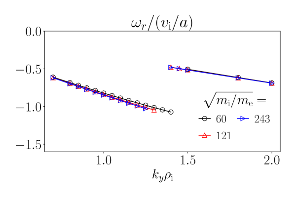
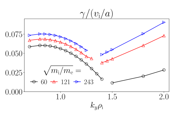
Figure 12: The real frequency $\omega_{{\rm{r}}}$ and growth rate $\gamma$ spectra as a function of $k_{y}\rho_{\rm{i}}$ and the expansion parameter $\left({m_{\rm{i}}}/{m_{\rm{e}}}\right)^{1/2}\propto\beta_{\rm{e}}^{-1}$, near the transition between the MTM mode branch (left of the discontinuity in $\omega_{{\rm{r}}}$) and the electrostatic mode branch (right of the discontinuity). Compare to figure 2. The boundary between the two types of modes remains almost constant in $k_{y}\rho_{\rm{i}}$ as the expansion parameter $\left({m_{\rm{i}}}/{m_{\rm{e}}}\right)^{1/2}$ is varied by a factor of 4. Since each value of $k_{y}\rho_{\rm{i}}$ corresponds to a unique value of $\beta^{\rm eff}$, a critical $\beta^{\rm eff}$ marks the boundary between the electromagnetic and the electrostatic modes.

The asymptotic theory predicts that $\beta_{\rm{e}}$ enters the dispersion relation only through $\beta^{\rm eff}$, an effective $\beta_{\rm{e}}$ that is defined by equation (33). This is a strong insight that we now proceed to test.

First, we examine the transition between the extended electrostatic modes and the MTM observed in figure 2. In figure 12, we plot the result of simulations around the transition in $k_{y}\rho_{\rm{i}}$, for different $\left({m_{\rm{i}}}/{m_{\rm{e}}}\right)^{1/2}$ and fixed $\theta_{0}=0$. As with the other $\left({m_{\rm{i}}}/{m_{\rm{e}}}\right)^{1/2}$ scans presented in this paper, we scale $\beta_{\rm{e}}\propto\left(m_{\rm{e}}/m_{\rm{i}}\right)^{1/2}$ in the scan so that $\beta^{\rm eff}$ is held constant at each $k_{y}\rho_{\rm{i}}$. We note that the transition in $k_{y}\rho_{\rm{i}}$ remains close to $k_{y}\rho_{\rm{i}}\approx 1.4$ even as $\left({m_{\rm{i}}}/{m_{\rm{e}}}\right)^{1/2}$ is varied by a factor of 4. Since there is a unique correspondance between $\beta^{\rm eff}$ and $k_{y}\rho_{\rm{i}}$ for $\beta_{\rm{e}}\propto\left(m_{\rm{e}}/m_{\rm{i}}\right)^{1/2}$, this proves that the transition in $k_{y}\rho_{\rm{i}}$ occurs at a fixed critical $\beta^{\rm eff}\sim 1$. In other words, the critical $\beta_{\rm{e}}$ for the onset of MTM instability scales with $\left(m_{\rm{e}}/m_{\rm{i}}\right)^{1/2}$.

Second, we test the detailed geometrical dependence of $\beta^{\rm eff}$ on the function $G(\theta_{0})$, defined by equation (34). Since the only leading-order dependence of the modes on $\theta_{0}$ enters through $\beta^{\rm eff}$, we would expect that varying $\theta_{0}$ would have the same effect as varying $\beta_{\rm{e}}$ by an appropriate amount. We test this hypothesis by performing a scan in $\beta_{\rm{e}}$ at fixed $(k_{y}\rho_{\rm{i}},\theta_{0})=(0.8,0.0)$ for the physical mass ratio $\left(m_{\rm{e}}/m_{\rm{i}}\right)^{1/2}=1/61$. In figure 13, we show the result of calculating the dimensionless frequency $\hat{\omega}=\hat{\omega}_{{\rm{r}}}+{\rm{i}}\hat{\gamma}$ as a function of $\beta^{\rm eff}$, with all other parameters in equation (39) held fixed. The range of the $\beta^{\rm eff}$ scan is limited by the appearance of competing instabilities. Below $\beta^{\rm eff}\lesssim 3$ the fastest growing instability is the electrostatic electron-driven mode, whereas for $\beta^{\rm eff}\gtrsim 15$ a highly localised mode in $\theta$ appears with a $\omega_{{\rm{r}}}$ in the ion diamagnetic direction. We use the data in figure 13 to obtain $\gamma(\beta^{\rm eff})$ and $\omega_{{\rm{r}}}(\beta^{\rm eff})$ for the mode at $\theta_{0}=0$. These fits can then be used to estimate the growth rate and frequency dependence on $\theta_{0}$ simply by computing $\beta^{\rm eff}(\theta_{0})$ for all $\theta_{0}$, using the definition (33). In figure 14 we compare these model predictions against gyrokinetic simulation results from GS2: we see excellent agreement for all $\theta_{0}$. This procedure starts to break down for $k_{y}\rho_{\rm{i}}$ too small, but works well for any $k_{y}\rho_{\rm{i}}$ that is sufficiently close to the electromagnetic-electrostatic mode transition highlighted in figures 2 and 12. This is likely a result of the fact that the asymptotic theory is valid only when $\beta_{\rm{e}}\sim\left(m_{\rm{e}}/m_{\rm{i}}\right)^{1/2}$ – when $\beta_{\rm{e}}$ approaches values of order unity ($\beta^{\rm eff}\sim\left({m_{\rm{i}}}/{m_{\rm{e}}}\right)^{1/2}\gg 1$) then a different high-$\beta$ asymptotic theory is required.

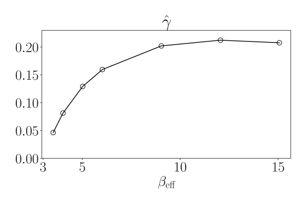
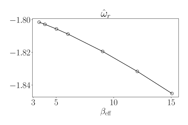
Figure 13: The dimensionless real frequency $\hat{\omega}_{{\rm{r}}}$ and the dimensionless growth rate $\hat{\gamma}$, defined through $\hat{\omega}=\hat{\omega}_{{\rm{r}}}+{\rm{i}}\hat{\gamma}$ and equation (39), plotted as a function of $\beta^{\rm eff}$, at fixed geometry, profiles, and $\hat{\nu}=0.797$ ($a\nu_{\rm{ee}}/v_{\rm{i}}=0.303$). The data is generated through a scan in $\beta_{\rm{e}}=[0.0289,0.124]$ at fixed $(k_{y}\rho_{\rm{i}},\theta_{0})=(0.8,0.0)$ and $\left(m_{\rm{e}}/m_{\rm{i}}\right)^{1/2}=1/61$. Whilst the frquency $\hat{\omega}_{{\rm{r}}}$ is almost independent of $\beta^{\rm eff}$, the dependence of $\hat{\gamma}$ on $\beta^{\rm eff}$ matches the predictions of the asymptotic theory: the critical $\beta^{\rm eff}$ is of order unity, and $\hat{\gamma}$ appears to approach a constant for a small range of $\beta^{\rm eff}$ as $\beta^{\rm eff}$ becomes large.

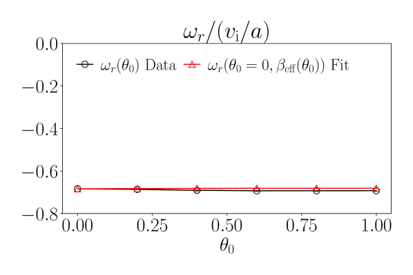
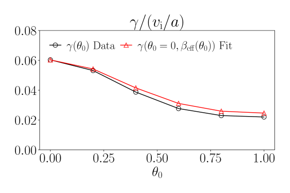
Figure 14: The real frequency $\omega_{{\rm{r}}}$ and growth rate $\gamma$ of the MTM at $k_{y}\rho_{\rm{i}}=0.8$, as a function of $\theta_{0}$. We compare two methods of computing the growth rate. First, the result of calculating $\omega_{{\rm{r}}}(\theta_{0})$ and $\gamma(\theta_{0})$ directly with GS2  using the nominal values of $\beta_{\rm{e}}$ in the MAST equilibrium. Second, noting that $\theta_{0}$ only enters the dispersion relation (39) through $\beta^{\rm eff}$, the result of using predictions for $\omega_{{\rm{r}}}$ and $\gamma$ based on the values of $\omega_{{\rm{r}}}(\theta_{0}=0,\beta^{\rm eff})$ and $\gamma(\theta_{0}=0,\beta^{\rm eff})$ and the value of $\beta^{\rm eff}(\theta_{0})$. The excellent agreement of the two curves suggests that the matching condition (30) is the correct one to describe the microinstabilities in MAST discharge #6252.

6 Discussion

In this paper, we have proposed a model for electron-driven electromagnetic linear instabilities that are localised to mode-rational surfaces, in the limit of $\beta_{\rm{e}}\sim k_{y}\rho_{\rm{e}}\sim\left(m_{\rm{e}}/m_{\rm{i}}\right)^{1/2}\ll 1$. The model consists of the orbit-averaged equations (11), (16), and (18) for the electron current layer, and a matching condition, equation (30), that connects the current layer to the large scale electromagnetic perturbation. Physically, the matching condition represents the streaming of electrons along perturbed magnetic field lines at large spatial scales: the magnetic field perturbations reconnect the equilibrium field lines and are driven by current carried by the electrons near the mode rational surface. The binormal scale of the mode $k_{y}\rho_{\rm{i}}\sim 1$ means that the radial width of the mode is of order $\rho_{\rm{i}}$, whilst the current layer is taken to be of order $\rho_{\rm{e}}$. As such, nonlocal physics due to the radial variation of equilibrium quantities of the scale of $a\gg\rho_{\rm{i}}\gg\rho_{\rm{e}}$ is neglected.

Besides the orderings (1) and (2), no further assumptions are made in deriving the model. Hence, the model is valid in arbitrary axisymmetric toroidal geometry and can treat the strong shaping observed in spherical tokamaks, and include a trapped particle response. Passing electrons are critical to the mode, since only passing electrons carry the current that can drive reconnection. Trapped electrons can contribute to the drive of the instability by dragging on passing particles through interparticle collisions [39]. However, numerical investigations into the role of trapped particles in MTMs show that trapped particles may be stabilising or destabilising [10].

The model makes the prediction that the dispersion relation has the form given by equation (39). As a consequence, we observe that $\beta_{\rm{e}}$ only appears through the parameter $\beta^{\rm eff}$, defined by equation (33). Physically, the parameter $\beta^{\rm eff}$ determines how the binormal wavenumber and the shaping in the magnetic geometry affects the amount by which electrons are forced to cross equilibrium magnetic field lines, and hence drive reconnection. The amount of field-line-crossing and the form of $\beta^{\rm eff}$ is determined by the size of the surface-averaged radial magnetic field induced by a given electron current from the rational-surface layer, see equations (27) and (29). We revisit MAST discharge #6252 [10], and we find that the MTMs there well satisfy the predictions made by the asymptotic theory. In particular, we are able to verify that $\beta^{\rm eff}$ accounts for the variation of the growth rate of the fastest-growing MTM mode in $\theta_{0}$. We also observe an electrostatic electron-driven mode with extended ballooning tails, similar to those observed in other magnetic geometries [31, 32].

The fact that we are able to identify a $\beta^{\rm eff}$ that takes into account the shaping of the local flux surface means that the model has the potential to make an immediate impact on transport modelling. In principle, nonlinear simulations of MTM-driven turbulence are required to evaluate heat fluxes in discharges that have MTMs appearing in the linear $k_{y}$ spectra. However, there have been persistent problems saturating this kind of turbulence – very few saturated MTM-driven turbulence simulations have been reported in the literature [35, 40, 41, 42]. One possible route to turbulence saturation is via equilibrium flow shear [43, 44, 45], which is effective provided that unstable microinstabilities are localised to $\theta_{0}\approx 0$ (the outboard midplane). Unfortunately, MTMs often have a healthy growth rate for all $-\pi<\theta_{0}\leq\pi$: the $\beta^{\rm eff}$ that we propose in this paper could act as a simple diagnostic to determine by how much the MTM growth rate $\gamma$ varies in $\theta_{0}$. The stronger the variation in $\beta^{\rm eff}$ between $\theta_{0}=0$ and $\pm\pi$, the more likely it is that the MTMs will be stable at the inboard side of the device, provided that $\beta^{\rm eff}\sim 1\ll\left({m_{\rm{i}}}/{m_{\rm{e}}}\right)^{1/2}$. This insight could be used to target flux surfaces in design studies which are particularly amenable to MTM turbulence saturation through equilibrium flow shear.

Further impact from the model could be derived from a numerical implementation of the equations, or an analytical solution in tractable asymptotic limits. A numerical implementation or analytical solution would be desirable because of the resolution requirements and computational costs associated with simulating long-wavelength MTMs with conventional gyrokinetic codes such as GS2. The large $\theta\sim(k_{y}\hat{s}\rho_{\rm{e}})^{-1}\gg 1$ extent in ballooning angle must be resolved at the same time as the fine geometrical structure in each $2\pi$ segment in ballooning angle. Short timescales due to electron parallel streaming must be resolved at the same time as the slower timescales associated with the drives of instability at wavelengths long compared to the electron gyroradius. The model that we propose could potentially achieve computational savings through two routes: first, by eliminating the fast timescales due to electron parallel streaming; and second, by allowing us to represent the fine $2\pi$ structure of the eigenmodes with an expansion of just a few poloidal harmonics.

The authors are grateful for productive discussions with T. Adkins, A. A. Schekochihin, A. Zocco, P. Helander, J. Larakers, D. Kennedy, R. Gaur, M. Anastopoulos-Tzanis, J. Maurino-Alperovich, S. Trinczek and G. Acton. This work has received funding from EPSRC [Grant Number EP/R034737/1]. This work was supported by the U.S. Department of Energy under contract number DE-AC02-09CH11466. The United States Government retains a non-exclusive, paid-up, irrevocable, world-wide license to publish or reproduce the published form of this manuscript, or allow others to do so, for United States Government purposes. The author acknowledges the use of the EUROfusion High Performance Computer (Marconi-Fusion) under projects OXGK and MULTISCA. This work made use of computational support by CoSeC, the Computational Science Centre for Research Communities, through CCP Plasma (EP/M022463/1) and HEC Plasma (EP/R029148/1). The simulations were performed using the GS2 branch https://bitbucket.org/gyrokinetics/gs2/branch/ms_pgelres, with commit ade5780. The data that support the findings of this study are available upon reasonable request from the authors. The GS2 input files used to perform the gyrokinetic simulations in this study are publicly available [46].

Appendix A The $k_{r}\rho_{\rm{e}}\sim 1$ scale

The expansion in the inner region is carried out in powers of $\left(m_{\rm{e}}/m_{\rm{i}}\right)^{1/2}\sim k_{y}\hat{s}\rho_{\rm{e}}\ll 1$. At the leading order in the expansion of equation (4), we find a balance between parallel streaming and the radial magnetic drift:

$$v_{\|}\bm{b}\cdot\nabla\theta\frac{\partial h_{{\rm{e}}}{}^{(0)}}{\partial\theta}-{\rm{i}}k_{\alpha}\chi q^{\prime}\bm{v}_{\rm{M,e}}\cdot\nabla\psi\;h_{{\rm{e}}}{}^{(0)}=0.$$ (42)

In equation (42), we have introduced $\chi=\theta$ where the ballooning angle appears secularly in the gyrokinetic equation. We treat $\theta$ and $\chi$ as independent variables in a multi-scale expansion, and we preserve $\theta$ as the argument of periodic functions.

Using the identity for the radial magnetic drift [47, 48],

$$\bm{v}_{\rm{M,e}}\cdot\nabla\psi=v_{\|}\bm{b}\cdot\nabla\theta\frac{\partial}{\partial\theta}\left(\frac{Iv_{\|}}{\Omega_{\rm{e}}}\right),$$ (43)

allows us to integrate equation (42) using an integrating factor $\exp{\left[-{\rm{i}}k_{\alpha}q^{\prime}\chi Iv_{\|}/\Omega_{\rm{e}}\right]}$, and obtain the relationship (9), in terms of the coordinate $z=k_{y}\hat{s}|\rho_{\rm{e}}^{\scriptsize\rm{ref}}|\chi$. At first order in the expansion the leading-order source due to the fields $\mathcal{S}_{{\rm e}}=-{\rm{i}}(\omega_{\ast,{\rm{e}}}-\omega)J_{0{\rm{e}}}e\phi F_{0e}/T_{\rm{e}}$ enters into the right hand side of the electron gyrokinetic equation. We have that

$$v_{\|}\bm{b}\cdot\nabla\theta\left(\frac{\partial h_{{\rm{e}}}{}^{(0)}}{\partial\chi}+\frac{\partial h_{{\rm{e}}}{}^{(1)}}{\partial\theta}\right)-{\rm{i}}k_{\alpha}\chi q^{\prime}\bm{v}_{\rm{M,e}}\cdot\nabla\psi\;h_{{\rm{e}}}{}^{(1)}$$

$$+{\rm{i}}\left(k_{\alpha}\bm{v}_{\rm{M,e}}\cdot(\nabla\alpha+\theta\nabla q)-\omega\right)h_{{\rm{e}}}{}^{(0)}-C^{\rm{GK}}_{\rm{e}}\left[h_{{\rm{e}}}{}^{(0)}\right]=\mathcal{S}_{{\rm e}}.$$ (44)

To close equation (44), in the passing part of phase space, we must impose $2\pi$-periodicity in $\theta$ on $h_{{\rm{e}}}{}^{(1)}$, i.e., $h_{{\rm{e}}}{}^{(1)}(\chi,\theta)=h_{{\rm{e}}}{}^{(1)}(\chi,\theta+2\pi)$. In the trapped part of phase space we must impose that $h_{{\rm{e}}}{}^{(1)}$ satisfies the bounce condition for trapped particles that $h_{{\rm{e}}}(\theta^{\pm}_{b},\sigma=1)=h_{{\rm{e}}}(\theta^{\pm}_{b},\sigma=-1)$ at the upper and lower bounce points $\theta^{\pm}_{b}$. This is achieved by multiplying equation (44) by the factor $\exp{\left[-{\rm{i}}k_{\alpha}q^{\prime}\chi Iv_{\|}/\Omega_{\rm{e}}\right]}$, applying the transit and bounce averages, defined by equations (12) and (17), respectively, to find the solvability conditions on $h_{{\rm{e}}}{}^{(0)}$. After normalising the results, using the coordinate $z=k_{y}\hat{s}|\rho_{\rm{e}}^{\scriptsize\rm{ref}}|\chi$, we have the equations (11) and (16).

Appendix B The electron drift-kinetic collision operator

In this appendix, we explicitly define the drift-kinetic collision operator appearing in equation (14). The drift-kinetic operator

$$\mathcal{C}\left[f\right]=C_{\rm{ee}}\left[f\right]+C_{\rm{ei}}\left[f\right],$$ (45)

where $f=f(\bm{v})$, $C_{\rm{ee}}[\cdot]$ is the linearised electron landau self-collision operator, and $C_{\rm{ei}}\left[\cdot\right]$ is the collision operator resulting from electron-ion collisions.

The landau self-collision operator $C_{\rm{ee}}\left[f\right]$ is defined by

$$C_{\rm{ee}}\left[f\right]=\frac{\nu_{\rm{ee}}v_{\rm{e}}^{3}}{2}\frac{\partial}{\partial\bm{v}}\cdot\int\frac{F_{0e}F_{0{\rm{e}}}^{\prime}}{n_{\rm{e}}}\bm{U}(\bm{v}-\bm{v}^{\prime})\cdot\left(\frac{\partial}{\partial\bm{v}}\left(\frac{f}{F_{0e}}\right)-\frac{\partial}{\partial\bm{v}^{\prime}}\left(\frac{f^{\prime}}{F_{0{\rm{e}}}^{\prime}}\right)\right)\;d^{3}\bm{v}^{\prime},$$ (46)

where the electron self-collision frequency $\nu_{\rm{ee}}$ is defined through equation (40), with the shorthand notation $f=f(\bm{v})$, $f^{\prime}=f(\bm{v}^{\prime})$, $F_{0e}=F_{0e}(\bm{v})$, $F_{0{\rm{e}}}^{\prime}=F_{0e}(\bm{v}^{\prime})$,

$$\bm{U}(\bm{v}-\bm{v}^{\prime})=\frac{\bm{I}|\bm{v}-\bm{v}^{\prime}|^{2}-(\bm{v}-\bm{v}^{\prime})(\bm{v}-\bm{v}^{\prime})}{|\bm{v}-\bm{v}^{\prime}|^{3}},$$ (47)

and $\bm{I}$ the identity matrix. Similarly, the electron-ion collision operator is defined by

$${C_{\rm{ei}}\left[f\right]=\frac{\nu_{\rm{ei}}v_{\rm{e}}^{3}}{2}\frac{\partial}{\partial\bm{v}}\cdot\left(\frac{v^{2}\bm{I}-\bm{v}\bm{v}}{v^{3}}\cdot\frac{\partial f}{\partial\bm{v}}\right),}$$ (48)

with the electron-ion collision frequency $\nu_{\rm{ei}}$ defined by equation (40). Note that the ion mean velocity does not appear in equation (48) because the nonadiabatic response of ions is small for $k_{r}\rho_{\rm{i}}\gg 1$.

Appendix C The $k_{r}\delta_{\rm{e}}\sim 1$ scale for $\beta_{\rm{e}}\ll 1$

In the $\beta_{\rm{e}}$ ordering (2), the electron inertial scale $\delta_{\rm{e}}=\rho_{\rm{e}}/\sqrt{\beta}$ is intermediate to the ion and electron gyroradius scales, i.e., $\rho_{\rm{e}}\ll\delta_{\rm{e}}\ll\rho_{\rm{i}}$. Since we assume that $k_{y}\rho_{\rm{i}}\sim 1$ and $\hat{s}\sim 1$, to treat the scale of $k_{r}\delta_{\rm{e}}\sim 1$ we must consider large ballooning angles in the range

$$\theta\sim(k_{y}\hat{s}\delta_{\rm{e}})^{-1}\sim\left(\frac{m_{\rm{i}}}{m_{\rm{e}}}\right)^{1/4}\gg 1.$$ (49)

We use a similar multi-scale expansion as used in A to derive the drift-orbit-averaged equations in the $k_{r}\delta_{\rm{e}}\sim 1$ region. Here, we expand in powers of $\left({m_{\rm{e}}}/{m_{\rm{i}}}\right)^{1/4}$, and we take $\theta\sim\left({m_{\rm{i}}}/{m_{\rm{e}}}\right)^{1/4}$. We introduce the independent variable $\chi=\theta$ where ballooning angle appears securlarly in the gyrokinetic equation, and we reserve $\theta$ for argument of periodic functions. We estimate the sizes of terms in the electron gyrokinetic equation using the non-dimensionalised Ampère’s law, equation (19), and the basic ordering (23).

At leading-order in the expansion we find that

$$v_{\|}\bm{b}\cdot\nabla\theta\frac{\partial h_{{\rm{e}}}{}^{(0)}}{\partial\theta}=0,$$ (50)

i.e., $h_{{\rm{e}}}{}^{(0)}=h_{{\rm{e}}}{}^{(0)}(\chi,\varepsilon,\lambda,\sigma)$ is independent of $2\pi$-geometric variation through $\theta$. At first-order in the expansion, we find that $h_{{\rm{e}}}{}^{(0)}$ is also independent of $\chi$:

$$v_{\|}\bm{b}\cdot\nabla\theta\left(\frac{\partial h_{{\rm{e}}}{}^{(0)}}{\partial\chi}+\frac{\partial h_{{\rm{e}}}{}^{(1/2)}}{\partial\theta}\right)-{\rm{i}}k_{\alpha}\chi q^{\prime}\bm{v}_{\rm{M,e}}\cdot\nabla\psi\;h_{{\rm{e}}}{}^{(0)}=0.$$ (51)

Applying the transit average $\left\langle{\cdot}\right\rangle^{\rm{t}}$, defined by equation (12), and using the identity (43), we find that

$$\frac{\partial h_{{\rm{e}}}{}^{(0)}}{\partial\chi}=0,$$ (52)

i.e., in fact, $h_{{\rm{e}}}{}^{(0)}=h_{{\rm{e}}}{}^{(0)}(\varepsilon,\lambda,\sigma)$.

This discussion shows that the leading-order passing electron distribution function is constant across the intermediate region where $k_{r}\delta_{\rm{e}}\sim 1$. The leading-order passing electron distribution function at $k_{r}\delta_{\rm{e}}\sim 1$ is determined by the incoming boundary conditions that are imposed on the $k_{r}\delta_{\rm{e}}\sim 1$ region from matching to the $k_{r}\rho_{\rm{i}}\sim 1$ and $k_{r}\rho_{\rm{e}}\sim 1$ regions. This comes about because in the ordering (1), electron parallel streaming dominates over the sources in the gyrokinetic equation at this scale.

Appendix D Numerical resolutions

The simulations presented in sections 4 and 5 of this paper use the following common set of numerical resolutions: the timestep size is taken to be $\Delta t=0.05/k_{y}\rho_{\rm{i}}$; we take $n_{\theta}=33$ points per $2\pi$ element in the ballooning angle grid; $n_{\lambda}=27$ points in the pitch angle grid, which is formed with a Radau-Gauss grid for passing particles and an unevenly spaced grid for trapped particles; and $n_{\varepsilon}=24$ points in the spectral energy grid [49]. The number of $2\pi$ elements in the ballooning grid $n_{2\pi}$ is chosen to be large enough to resolve the eigenmode and frequency. The ballooning-space extent of electron-driven modes varies with $k_{y}\rho_{\rm{e}}$, leading to different requirements on $n_{2\pi}$ for modes of different $\left(m_{\rm{e}}/m_{\rm{i}}\right)^{1/2}$ and $k_{y}\rho_{\rm{i}}$. For the mode at $k_{y}\rho_{\rm{i}}=0.1$ and $\left(m_{\rm{e}}/m_{\rm{i}}\right)^{1/2}=1/61$ in figure 3, $n_{2\pi}=399$ is required, whereas for the modes at $k_{y}\rho_{\rm{i}}=0.8$ ($2.2$) $n_{2\pi}=79$ ($39$) is found to be adequate. When $\left(m_{\rm{e}}/m_{\rm{i}}\right)^{1/2}$ is varied at fixed $k_{y}\rho_{\rm{i}}$, we increase $n_{2\pi}\propto\left({m_{\rm{i}}}/{m_{\rm{e}}}\right)^{1/2}$.

References

• [1] Strauss H, Park W, Monticello D, White R, Jardin S, Chance M, Todd A and Glasser A 1980 Nucl. Fusion 20 635–642
• [2] Lortz D and Nührenberg J 1978 Physics Letters A 68 49–50
• [3] Tang W M, Connor J W and Hastie R J 1980 Nucl. Fusion 20 1439–1453
• [4] Hastie R and Hesketh K 1981 Nucl. Fusion 21 651–656
• [5] Aleynikova K and Zocco A 2017 Phys. Plasmas 24 092106
• [6] Drake J F, Gladd N T, Liu C S and Chang C L 1980 Phys. Rev. Lett. 44 994–997
• [7] Gladd N T, Drake J F, Chang C L and Liu C S 1980 Phys. Fluids 23 1182–1192
• [8] Drake J F, Antonsen T M, Hassam A B and Gladd N T 1983 Phys. Fluids 26 2509–2528
• [9] Connor J W, Cowley S C and Hastie R J 1990 Plasma Phys. Control. Fusion 32 799–817
• [10] Applegate D J, Roach C M, Connor J W, Cowley S C, Dorland W, Hastie R J and Joiner N 2007 Plasma Phys. Control. Fusion 49 1113–1128
• [11] Zocco A, Loureiro N F, Dickinson D, Numata R and Roach C M 2015 Plasma Phys. Control. Fusion 57 065008
• [12] Hamed M, Muraglia M, Camenen Y, Garbet X and Agullo O 2019 Phys. Plasmas 26 092506
• [13] Patel B, Dickinson D, Roach C and Wilson H 2021 Nucl. Fusion 62 016009
• [14] Moradi S, Pusztai I, Guttenfelder W, Fülöp T and Mollén A 2013 Nucl. Fusion 53 063025
• [15] Dickinson D, Roach C M, Saarelma S, Scannell R, Kirk A and Wilson H R 2013 Plasma Phys. Control. Fusion 55 074006
• [16] Predebon I and Sattin F 2013 Phys. Plasmas 20 040701
• [17] Geng C, Dickinson D and Wilson H 2020 Plasma Phys. Control. Fusion 62 085009
• [18] Furth H P, Killeen J and Rosenbluth M N 1963 Phys. Fluids 6 459–484
• [19] Drake J F and Lee Y C 1977 Phys. Fluids 20 1341–1353
• [20] Cowley S C, Kulsrud R M and Hahm T S 1986 Phys. Fluids 29 3230–3244
• [21] Zocco A and Schekochihin A A 2011 Phys. Plasmas 18 102309
• [22] Connor J W, Hastie R J and Zocco A 2012 Plasma Phys. Control. Fusion 54 035003
• [23] Roach C M, Applegate D J, Connor J W, Cowley S C, Dorland W D, Hastie R J, Joiner N, Saarelma S, Schekochihin A A, Akers R J, Brickley C, Field A R, Valovic M and the MAST Team 2005 Plasma Physics and Controlled Fusion 47 B323–B336
• [24] Roach C M, Abel I G, Akers R J, Arter W, Barnes M, Camenen Y, Casson F J, Colyer G, Connor J W, Cowley S C, Dickinson D, Dorland W, Field A R, Guttenfelder W, Hammett G W, Hastie R J, Highcock E, Loureiro N F, Peeters A G, Reshko M, Saarelma S, Schekochihin A A, Valovic M and Wilson H R 2009 Plasma Phys. Control. Fusion 51 124020
• [25] Bourdelle C, Hoang G, Litaudon X, Roach C and Tala T 2005 Nucl. Fusion 45 110–130
• [26] Citrin J, Garcia J, Görler T, Jenko F, Mantica P, Told D, Bourdelle C, Hatch D R, Hogeweij G M D, Johnson T, Pueschel M J, Schneider M and Contributors J E 2015 Plasma Phys. Control. Fusion 57 014032
• [27] Zocco A, Helander P and Connor J W 2015 Plasma Phys. Control. Fusion 57 085003
• [28] Ishizawa A, Urano D, Nakamura Y, Maeyama S and Watanabe T H 2019 Phys. Rev. Lett. 123 025003
• [29] Catto P J 1978 Plasma Phys. 20 719
• [30] Catto P J, Tang W M and Baldwin D E 1981 Plasma Physics 23 639–650
• [31] Hallatschek K and Dorland W 2005 Phys. Rev. Lett. 95 055002
• [32] Hardman M R, Parra F I, Chong C, Adkins T, Anastopoulos-Tzanis M S, Barnes M, Dickinson D, Parisi J F and Wilson H 2022 Plasma Phys. Control. Fusion 64 055004
• [33] Connor J W, Hastie R J and Taylor J B 1979 Proceedings of the Royal Society of London. A. Mathematical and Physical Sciences 365 1–17
• [34] Kotschenreuther M, Rewoldt G and Tang W 1995 Computer Physics Communications 88 128 – 140
• [35] Guttenfelder W, Candy J, an W M Nevins S M K, Wang E, Bell R E, Hammett G, LeBlanc B P, Mikkelsen D R and Yuh H 2011 Phys. Rev. Lett. 106 155004
• [36] Miller R L, Chu M S, Greene J M, Lin-Liu Y R and Waltz R E 1998 Phys. Plasmas 5 973–978
• [37] Barnes M, Abel I G, Dorland W, Ernst D R, Hammett G W, Ricci P, Rogers B N, Schekochihin A A and Tatsuno T 2009 Phys. Plasmas 16 072107
• [38] Hazeltine R D and Meiss J D 2003 Plasma Confinement (New York: Dover)
• [39] Catto P J and Rosenbluth M N 1981 Phys. Fluids 24 243–255
• [40] Doerk H, Jenko F, Görler T, Told D, Pueschel M J and Hatch D R 2012 Phys. Plasmas 19 055907
• [41] Maeyama S, Watanabe T H and Ishizawa A 2017 Phys. Rev. Lett. 119 195002
• [42] J A C, McMillan B and Pueschel M J 2022 arXiv:2207.09211
• [43] Newton S L, Cowley S C and Loureiro N F 2010 Plasma Phys. Control. Fusion 52 125001
• [44] Highcock E G, Barnes M, Schekochihin A A, Parra F I, Roach C M and Cowley S C 2010 Phys. Rev. Lett. 105 215003
• [45] Barnes M, Parra F I, Highcock E G, Schekochihin A A, Cowley S C and Roach C M 2011 Phys. Rev. Lett. 106 175004
• [46] Hardman M R, Parra F I, Patel B S, Roach C M, Ruiz J R, Barnes M, Dickinson D, Dorland W, Parisi J F, St-Onge D and Wilson H 2023 Zenodo URL https://doi.org/10.5281/zenodo.7638831
• [47] Hinton F L and Hazeltine R D 1976 Rev. Mod. Phys. 25 239–308
• [48] Helander P and Sigmar D J 2002 Collisional transport in magnetized plasmas (Cambridge: Cambridge University Press)
• [49] Barnes M, Dorland W and Tatsuno T 2010 Phys. Plasmas 17 032106