Constraining Scale Dependent Growth with Redshift Surveys

Abstract

Ongoing and future redshift surveys have the capability to measure the growth rate of large scale structure at the percent level over a broad range of redshifts, tightly constraining cosmological parameters. Beyond general relativity, however, the growth rate in the linear density perturbation regime can be not only redshift dependent but scale dependent, revealing important clues to modified gravity. We demonstrate that a fully model independent approach of binning the gravitational strength $G_{\rm eff}(k,z)$ matches scalar-tensor results for the growth rate $f\sigma_{8}(k,z)$ to $0.02\%$–$0.27\%$ rms accuracy. For data of the quality of the Dark Energy Spectroscopic Instrument (DESI) we find the bin values can be constrained to 1.4%–28%. We also explore the general scalar-tensor form, constraining the amplitude and past and future scalaron mass/shape parameters. Perhaps most interesting is the strong complementarity of low redshift peculiar velocity data with DESI-like redshift space distortion measurements, enabling improvements up to a factor 6–7 on 2D joint confidence contour areas. Finally, we quantify some issues with gravity parametrizations that do not include all the key physics.

I Introduction

Cosmic growth of large scale structure is a competition between increased clustering amplitude driven by gravity and damped evolution due to expansion, exacerbated by cosmic acceleration. Thus the growth, and more incisively the growth rate, can reveal important characteristics of gravitation and dark energy. The new generation of spectroscopic galaxy surveys measure redshift space distortions across wide areas of sky and broad redshift ranges, enabling precision estimates of the growth rate $f\sigma_{8}$.

Within general relativity these measurements translate directly to cosmic expansion history constraints, but the extra freedom within modified gravity means that redshift space distortions can serve as a critical probe of gravity (see, e.g., [1, 2, 3, 4] for early work). Moreover, with modified gravity there generally enters scale dependence in the growth rate, even in the linear density perturbation regime, a further signal of deviation from Einstein gravity. We focus here on constraining scale dependent growth, in as model independent a manner as practical, with the quality of data likely to be delivered by the current spectroscopic surveys such as from the Dark Energy Spectroscopic Instrument (DESI, [5, 6]). (While scale dependence can enter due to massive neutrinos, this has a specific scale and redshift dependence that can be fit, while scale dependence from, e.g., a warm dark matter component generally enters beyond the linear scales for viable models. Therefore we only explore scale dependence from modified gravity here.)

In Section II we investigate the evolution of the scale- and redshift-dependent cosmic growth rate $f\sigma_{8}(k,a)$ and explore the impact of the physics motivated scalar-tensor gravity form for the modified gravity strength, keeping it as model independent as reasonable. Section III then demonstrates that a wholly model independent form, using $2\times 3$ bins in scale and redshift, can provide an excellent approximation to the full form. We project constraints in Section IV for what DESI-quality data could enable to test gravity through scale dependent growth in these two approaches. Leverage from peculiar velocity low redshift observations is examined as well. Section V studies a coarser, but easier to be alerted to distinctions from general relativity, $2\times 2$ bin approach. In Section VI we summarize and conclude.

II Scale Dependent Growth

Galaxy redshift surveys use redshift space distortions to determine the growth rate factor

$$f\sigma_{8}(a)=fD\,\frac{\sigma_{8,0}}{D_{0}}=\frac{dD}{d\ln a}\,\frac{\sigma_{8,0}}{D_{0}}\ ,$$ (1)

where $D$ is the linear perturbation growth factor, $a$ is the expansion factor, and $\sigma_{8}$ the mass fluctuation amplitude; subscript 0 denotes the value today. Unlike for the logarithmic growth rate $f=d\ln D/d\ln a$, the evolution equation for $D$ is linear:

$$D^{\prime\prime}+D^{\prime}\left[2+\frac{1}{2}\left(\ln H^{2}\right)^{\prime}\right]-\frac{3}{2}DG_{m}\Omega_{m}(a)=0\ ,$$ (2)

where prime denotes a derivative with respect to $\ln a$.

It is convenient to break this second order equation into two coupled first order equations,

$$D^{\prime} = (fD)$$ (3)

$$(fD)^{\prime} = -(fD)\left[2+\frac{1}{2}\left(\ln H^{2}\right)^{\prime}\right]+\frac{3}{2}DG_{m}\Omega_{m}(a)\ .$$ (4)

Here $H(a)$ is the Hubble parameter $\dot{a}/a$, and $\Omega_{m}(a)$ is the matter density in units of the critical density. The factor $G_{m}$ is the gravitational coupling strength of matter, in units of Newton’s constant. In general relativity it is simply one.

However, in modified gravity $G_{m}$ can differ from one, and be both expansion factor (redshift) dependent and scale (wavemode) dependent. Since we work in the linear regime, linear perturbations at one wavenumber $k$ are independent of those at another. In general then we have $G_{m}(k,a)$, determining $f\sigma_{8}(k,a)$.

II.1 Modified Gravity

One could adopt a particular theory of modified gravity, with a certain functional form, and certain parameters within that form – e.g. $f(R)$ gravity of the Hu-Sawicki form with parameter $n=4$ – but the constraints derived from the data will then apply only to that specific case. We take a more model independent approach, using that in scalar-tensor theories the gravitational coupling to matter can be fairly generically written as [7, 8, 9, 10, 11, 12, 13, 14]

$$G_{m}=\frac{1+c\,\left(k/[aM(a)]\right)^{2}}{1+\left(k/[aM(a)]\right)^{2}}\ .$$ (5)

This comes directly from the Einstein field equations in the quasistatic regime, where precision observations can be made, and can be seen as well in both the effective field theory of dark energy approach [15] and property function approach, e.g. [16]. We take the scalaron mass to be given by

$$M(a)=M_{a}a^{-3}+M_{\rm dS}\ ,$$ (6)

which fits many models reasonably [17] (also see [18]), and guarantees a high redshift universe looking like that in general relativity. Since in general relativity $G_{m}=1$, we define $\delta G=G_{m}-1$. We refer to $c$ as the amplitude parameter and $M_{a}$ and $M_{\rm dS}$ as the shape parameters, since they govern the evolution of scale dependence. Note that at high redshift the scalaron mass is large, $M\approx M_{a}a^{-3}$, today $M(a=1)=M_{a}+M_{\rm dS}$, and in the future the scalaron mass freezes as the universe approaches a de Sitter state, $M(a)\to M_{\rm dS}$. Since today the expansion is not too far from the de Sitter state, i.e. $\Omega_{\rm de}\approx 0.7$, then we expect $M(a=1)=M_{a}+M_{\rm dS}$ to be not far from $M_{\rm dS}$. Thus $M_{a}\lesssim M_{\rm dS}$ is a reasonable value.

Consider a fiducial model of $c=4/3$, $M_{a}=0.05$, $M_{\rm dS}=0.05$. (All wavenumbers and masses are in $h$/Mpc units.) The value $c=4/3$ matches $f(R)$ gravity [11], and the value $M(a=1)=M_{a}+M_{\rm dS}=0.1$ gives a value for the Compton wavelength parameter [19] $B_{0}=2[H_{0}/M(a=1)]^{2}\approx 2.2\times 10^{-5}$. The exact translation of $B_{0}$ to the $f(R)$ parameter $f_{R0}$ is model dependent, but generally $f_{R0}\approx-B_{0}/(1-4)$. Thus the fiducial model has $f_{R0}\approx-10^{-5}$, toward the high end of what is allowed by current data, designed to stress test the ability of our binned approach to accurately fit the growth data. Finally note that the power $a^{-3}$ in Eq. (6) also stress tests our approach in that this is the shallowest power allowed: one requires $M(a\ll 1)\sim a^{\leq-3}$ [11, 20] to obtain the standard matter dominated Friedmann expansion equation behavior. Using the limit $M(a\ll 1)\sim a^{-3}$ keeps modifications stronger at earlier times and so makes fitting growth accurately with a small number of $\delta G$ bins more difficult.

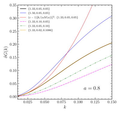
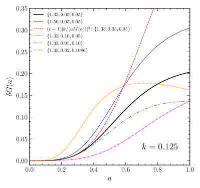
Figure 1: Modified gravitational strength deviations from GR are plotted as $\delta G$ vs $k$, at $a=0.8$ (left panel), and $\delta G$ vs $a$ at $k=0.125$ (right panel). The fiducial case of $c=4/3$, $M_{a}=M_{\rm dS}=0.05$ (bold black curve) and several variations as labeled by $(c,M_{a},M_{\rm dS})$ are shown, as well as an unmotivated power law rather than Padé polynomial case (dashed red).

Figure 1 shows $\delta G(k)$ for $a=0.8$, i.e. in the recent universe where the deviation from general relativity (GR) is larger, and $\delta G(a)$ for $k=0.125$, i.e. at a higher wavenumber where the deviation is larger. We illustrate the effects of changing the parameters one by one. Increasing the amplitude parameter $c$ of course scales $\delta G$ at all $k$ and $a$ (compare thin blue vs bold black curves). For the shape parameters entering the scalaron mass, recall that large mass increases the similarity to GR. Increasing the shape parameter $M_{a}$ greatly suppresses modifications until recently, for example we see that $\delta G$ is three times smaller at $a=0.5$ (for $k=0.125$) for $M_{a}=0.1$ rather than $M_{a}=0.05$ (compare dot dash purple vs bold black curves). The shape parameter $M_{\rm dS}$ changes the late time behavior; it is not until $a\gtrsim 0.5$ that increasing $M_{\rm dS}$ from 0.05 to 0.1 has an appreciable effect (dot dot dash green vs bold black).

There are two other points of interest to note. First, using a form like $G_{m}=1+ba^{s}$ is quite problematic. See the detailed analysis in [21], as well as [22] and the model independent approach of [23]. It gives very different behavior than the full Padé ratio of Eq. (5); this is particularly evident in the dashed red curve in Fig. 1. The basic issue is that it overweights late times (and high $k$) so that a constraint from late time data could be interpreted as an unrealistically tight limit on modified gravity. Recall that the Padé form originates from the Einstein field equations [7, 8, 9, 10, 12, 13, 14]; basically $G_{m}$ comes from $F_{1}$(metric potential) = $F_{2}$(matter fields), where $F_{i}$ are factors including space and time derivative terms, and matter fields include the scalar field perturbations; both sides involve $k^{2}$ corrections beyond leading order. Since $G_{m}$ arises from a ratio of the factors, using only a single polynomial rather than a Padé form is throwing away half the physics. This holds for any scalar-tensor theory. We can see from Fig. 1 that the discrepancy is already significant for $a\gtrsim 0.5$ or $k\gtrsim 0.06$.

Secondly, as mentioned the scalaron mass freezes approaching a dark energy dominated de Sitter state, $G_{m}\not\to c$ but rather gravity is eventually restored to GR, $G_{m}\to 1$ since $aM(a)\to aM_{\rm dS}$ and the factors multiplying the $k^{2}$ terms go to zero. The “phase space” evolution of $G_{m}$ for various modified gravity theories is discussed and illustrated in [17]. Whether $G_{m}$ reaches its fully modified value of $c$ before turning around and approaching back to 1 depends on the values of $M_{a}$ and $M_{\rm dS}$. We illustrate this in Fig. 1 with the dotted orange curve, where $M_{a}$ and $M_{\rm dS}$ are chosen to match $M(a=0.8)$ from the fiducial model (specifically, we use $M_{a}$=0.02, $M_{\rm dS}=0.1086$). Indeed, the left panel shows perfect overlap between those two cases, while the right panel shows that they coincide only at (the chosen) $a=0.8$. The turnaround is clearly seen: the dotted orange curve never exceeds $\delta G\approx 0.18$, well short of $c-1=0.33$. All of the curves (except the non-Padé one) will eventually turn around; it simply occurs later for smaller $M_{\rm dS}$.

II.2 Growth Rate

Given $G_{m}$, Eq. (5), one can then solve Eq. (4) and obtain the scale dependent growth rate $f\sigma_{8}(k,a)$ in the linear regime. Figure 2 shows $(f\sigma_{8}-f\sigma_{8}^{GR})/f\sigma_{8}^{GR}$ vs $a$ for various $k$, and vs $k$ for various $a$, for the fiducial modified gravity model, in a $\Lambda$CDM background with fractional matter density today $\Omega_{m}=0.3$. (Recall that the maximum equation of state deviation from $-1$ for many $f(R)$ theories is $|1+w|_{\rm max}\approx B_{0}/2\ll 1$ [24], so $\Lambda$CDM is an excellent approximation.) We normalize the amplitude to the same primordial density amplitude as GR (as measured by the cosmic microwave background), rather than to the present mass fluctuation amplitude $\sigma_{8,0}$ (which would cause deviations at high redshift).

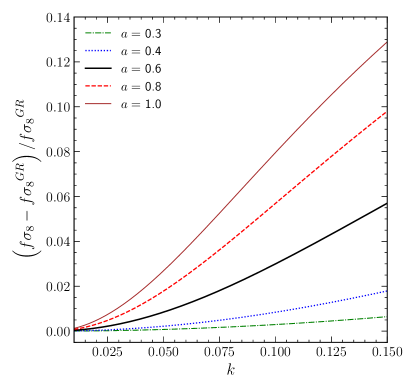
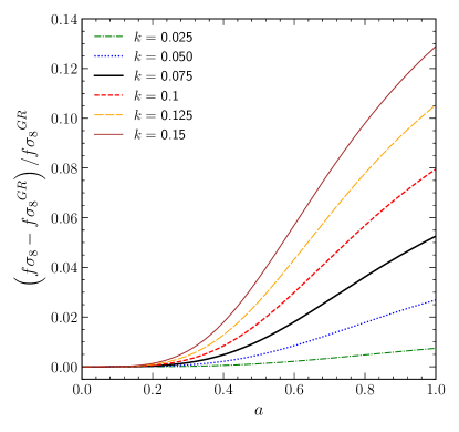
Figure 2: The fractional difference of $f\sigma_{8}$ relative to general relativity is plotted vs $k$, for various scale factors $a$ [left panel], and vs $a$ for various wavemodes $k$ [right panel].

The growth rate $f\sigma_{8}$ has less than 1% deviation from GR for the fiducial model earlier than about one efold before the present, $a\lesssim 0.37$, for $k<0.15$. Lower wavenumbers deviate later and with a smaller amplitude. Between $a=0.4$ ($z=1.5$) and $a=0.8$ ($z=0.25$), the deviation grows by a factor of $\sim 6$. Thus redshift space distortion data over a broad range of redshifts is highly useful. The deviation from GR in the growth rate increases with $k$, reaching 2–10% at $k=0.15$ for $a=0.4$–0.8, the range of near term precision redshift space distortion data. Thus we see that percent level measurements of $f\sigma_{8}$ will be required, somewhat eased by adding up measurements at many redshifts. It is important to remember that $f\sigma_{8}(k,a)$ is affected by all values $G_{m}(k,a^{\prime}\leq a)$; i.e. while modes evolve independently within the linear regime, modifications in the gravitational strength at earlier times affect the growth rate at later times (effectively changing the “momentum” of the growth, see [25]).

III Model Independent Fitting

Within scalar-tensor theories, we then have a three parameter fit $(c,M_{a},M_{\rm dS})$ for gravity that can be used for testing GR with growth rate data. This is a valid and useful approach, but while it is the most physical approach without adopting a specific gravity model it does have some drawbacks. One must solve the growth equation for each point in the parameter space, and there is some degeneracy. High values of $M(a)$, coming from either large $M_{a}$ or large $M_{\rm dS}$, are indistinguishable from GR (for a Monte Carlo fitting approach one might want to adopt priors on $1/M_{a}$, $1/M_{\rm dS}$ instead). Covariance between the parameters can only partially be ameliorated with data over a range of $k$ and $a$. Finally, while the Padé form is model independent within canonical scalar-tensor theories, we might want to test the framework itself.

Therefore we will also investigate an even more model independent approach, that of independent bin values of $G_{m}$ in $k$ and $a$. (One can also use node values for $G_{m}$ and interpolate between them, e.g. with linear or spline functions. This smoothness increases the ease of attaining a good fit to the exact form (see Sec. V) but also increases the covariance between bins and hence the interpretation of $G_{m}(z)$. In the spirit of “stress testing” the ability of bins to accurately give $f\sigma_{8}$ we use $G_{m}$ constant in bins.) We want to keep the number of bins small, but sufficient to both see the physics qualitatively and reproduce the growth rate with quantitative accuracy. Note that the bins are in $G_{m}$, giving the full, continuous function $f\sigma_{8}(k,a)$. (For some studies using gravity binned in scale and redshift, see [26, 27, 28, 29, 30, 31, 32, 33, 34, 35, 36, 37].)

Since we restrict ourselves to the quasilinear regime, we choose two bins in $k$: low $k=[0.01,0.1]$ and high $k=[0.1,0.15]$. Subdividing further would lead to increased covariance between parameters and weaker constraints. For expansion factor $a$, we recognize that models such as $f(R)$ have very rapid variation in their time dependence, e.g. $\delta G\sim a^{4}$ at low $k$, low $a$. This led [38] to adopt three bins in $a$ for accuracy, and we follow this procedure. We take bins, in redshift, of $z=[0,0.5]$, [0.5,1], and [1,3]. Again we emphasize that these are bins for $G_{m}$ and not in $f\sigma_{8}$. Although we saw that $f\sigma_{8}$ deviates from GR by less than 1% for $a<0.37$, we must allow $G_{m}$ to deviate earlier since those deviations affect all later $f\sigma_{8}$, even up to $z=0$. From Fig. 1 we see that $\delta G$ deviates by less than 1% at $a<0.25$, and set $G_{m}=1$ at $a<0.25$. Note that while $G_{m}$ is piecewise constant in bins, as we never take derivatives of $G_{m}$ then jumps at the bin boundaries do not cause difficulties for the calculation; smoothing the transitions was studied in [38] and found not to affect substantially the results.

From the $2\times 3$ binned values of $G_{m}$ we compute $\widehat{f\sigma_{8}}(k,a)$ and compare this to $f\sigma_{8}$ from the full, Padé functional form of $G_{m}$. Minimizing the variance of the fractional deviation $(\widehat{f\sigma_{8}}-f\sigma_{8})/f\sigma_{8}$ determines the optimal values for the binned $G_{m}$. Note that while each $k$ bin is independent from the others, since the growth equation does not couple modes in the linear regime, the evolution of $\widehat{f\sigma_{8}}$ at some $a$ does depend on $G_{m}$ at earlier $a$ as this affects $D(a)$, which has been integrated from the high redshift, GR initial conditions to $a$.

In more detail, we recognize that observational data will not have $f\sigma_{8}(k,a)$ at every $k$ with sufficient signal to noise (S/N) to test gravity, but rather one must assess $f\sigma_{8}$ for modes over some range. So as not to decrease the S/N of the data too much we choose two bins of $k$ in $f\sigma_{8}$, using $k=[0.01,0.1]$ and $k=[0.1,0.15]$. Since a deviation $\delta G$ at some $k$ leads to a deviation in $f\sigma_{8}$ at exactly that $k$ and no other, in the linear regime, it is convenient to take the $f\sigma_{8}$ bins in $k$ to be the same as the $G_{m}$ bins in $k$. Measurements would be quoted at some $k_{\rm eff}$ in each bin, which here we will simply take as the bin center, i.e. $k_{\rm eff}=0.055$, 0.125. (One could take into account the mode density, dependence of the power spectrum on $k$, spectrograph fiber collision weights [39], etc. to come up with a more sophisticated $k_{\rm eff}$ but we simply take the bin center.) In redshift, data is usually reported in fairly narrow redshift slices, approximating a continuous function for $f\sigma_{8}$ in terms of $a$, so we do not bin $f\sigma_{8}$ in $a$ (while $G_{m}$ values are defined in bins in $a$). However, the precision of redshift space distortion measurements degrades at $z<0.2$ where there is relatively little volume (but see Sec. IV.3 where we revisit this using peculiar velocity surveys). At high redshift, again the precision worsens due to observational difficulties. Therefore we carry out the optimization of $G_{m}(k,a)$ bins by minimizing the variance of deviations in $f\sigma_{8}$ over the range $z=[0.2,1.7]$. (Recall that $G_{m}$ at $z>1.7$ still affects $f\sigma_{8}$ over this whole range.)

Figure 3 shows the fractional residuals of the fit $(\widehat{f\sigma_{8}}-f\sigma_{8})/f\sigma_{8})$ vs $k$ for various values of $a$, and vs $a$ for various $k$. However, what is important are the results at the two values $k_{\rm eff}=0.055$ and 0.125 since $f\sigma_{8}(k_{\rm eff},a)$ is what the data will actually provide. These values are marked by the vertical lines in the left panel, and the solid curves in the right panel. We see that over the redshift range of the data, the binned $G_{m}$ approach succeeds in delivering accurate results, with the maximum deviation $\lesssim 0.1\%$ in the low $k$ bin, and $\lesssim 0.1\%$ in the high $k$ bin except right around $a=0.5$ (a $G_{m}$ bin boundary) where the maximum deviation is $\approx 0.6\%$. Changing from piecewise constant $G_{m}$ to a smoother form would reduce this deviation, but 0.6% is still sufficiently good as we will see the observational precision at this redshift is expected to be $\approx 2\%$ when the redshift space distortions are analyzed in two $k$ bins. The rms deviations are even smaller, as shown in Table 1.

Range	rms	max
low $k$, low $a$	0.07%	0.13%
low $k$, mid $a$	0.04%	0.13%
low $k$, high $a$	0.02%	0.04%
high $k$, low $a$	0.27%	0.64%
high $k$, mid $a$	0.22%	0.64%
high $k$, high $a$	0.06%	0.12%

Table 1: Fractional deviations on the growth rate $f\sigma_{8}$ computed using binned $G_{m}$ vs the exact form. Low/high $k$ refers to $k_{\rm eff}=0.055$, 0.125 respectively; low/mid/high $a$ refers to the ranges [0.37,0.5], [0.5,0.667], [0.667,0.833]. The rms and max columns give the rms and maximum deviations across those ranges of $a$.

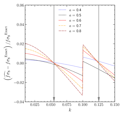
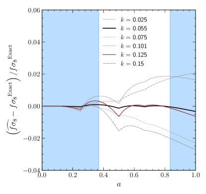
Figure 3: The fractional difference of $f\sigma_{8}$ using the optimized binned $G_{m}^{\rm bin}$ (giving $\widehat{f\sigma_{8}}$) vs using the exact modified gravity $G_{m}$ (giving $f\sigma_{8}^{\rm Exact}$) is plotted vs $k$ for various $a$ [left panel] and vs $a$ for various $k$ [right panel]. Only the values at $k_{\rm eff}=0.055$, 0.125 are observationally relevant (since $f\sigma_{8}$ data cannot be divided into more than two bins without losing too much precision). These are indicated with vertical lines in the left panel, and solid curves in the right panel. The observationally relevant (i.e. good data precision) range in $a$ is indicated by the unshaded region in the right panel.

While in Fig. 3 we show $(\widehat{f\sigma_{8}}-f\sigma_{8})/f\sigma_{8}$ at other values of $k$ than $k_{\rm eff}$, we again emphasize that the values at $k_{\rm eff}$ are what is important when comparing with data. The $G_{m}$ values obtained from our variance minimization are: $\delta G^{\rm bin}_{11}=0.0065$, $\delta G^{\rm bin}_{12}=0.031$, $\delta G^{\rm bin}_{13}=0.052$, $\delta G^{\rm bin}_{21}=0.029$, $\delta G^{\rm bin}_{22}=0.127$, $\delta G^{\rm bin}_{23}=0.158$, where $\delta G^{\rm bin}$ denotes $G_{m}^{\rm bin}-G^{GR}$ and the numerical indices give the bins of $G_{m}$ in $k$ and $a$ respectively, from low values of $k$ or $a$ to high. For example, $\delta G^{\rm bin}_{23}$ is the optimized binned deviation in gravity in the $G_{m}$ bin $k=[0.1,0.15]$, $a=[0.667,1]$. As expected there is a clear trend of strengthening gravity for increasing $k$ or $a$.

IV Projected Constraints

To estimate parameter constraints on the gravitational model we can employ the information matrix formalism, where the information matrix is

$$F_{ij} = \sum_{k_{\rm eff,n}}\sum_{z_{m}}\frac{\partial f\sigma_{8}(k_{\rm eff,n},z_{m})}{\partial p_{i}}\frac{\partial f\sigma_{8}(k_{\rm eff,n},z_{m})}{\partial p_{j}}$$ (7)

$$\qquad\times\frac{1}{[\sigma(k_{\rm eff,n},z_{m})f\sigma_{8}(k_{\rm eff,n},z_{m})]^{2}}\ ,$$ (8)

and the marginalized parameter constraints are given by the elements of $F^{-1}$, with the uncertainty on a parameter equal to the square root of its diagonal element, i.e. $\sigma(p_{i})=\sqrt{(F^{-1})_{ii}}$.

The set of data $f\sigma_{8}(k_{\rm eff,n},z_{m})$ are taken to follow those projected for the Dark Energy Spectroscopic Instrument (DESI), using only the redshift space distortion galaxy data. We include the redshift range $z_{m}=0.25,0.35,\dots 1.65$ where precision is strong, with the uncorrelated fractional precisions $\sigma(k_{\rm eff,n},z_{m})$ given by Tables 2.3 and 2.5 of [5]. We evaluate $f\sigma_{8}$ at $k_{\rm eff}=0.055$ and 0.125, reflecting that the observed data must extend over a range, here respectively $k=[0.01,0.1]$ and $k=[0.1,0.15]$, to obtain good precision. For the lower $k$ bin, we use the column in the $k_{\rm max}=0.1$ column of those tables; for the higher $k$ bin we use $\sigma_{[0.1,0.15]}=1.5(\sigma_{k_{\rm max}=0.2}^{-2}-\sigma_{k_{\rm max}=0.1}^{-2})^{-1/2}$, where the 1.5 factor is a reasonable approximation (generally it ranges from $\sim 1.3-1.7$ depending on redshift and treatment of quasilinearity) for the uncertainty for the range $k=[0.1,0.15]$ vs [0.1,0.2]. The background cosmology is taken as $\Lambda$CDM with $\Omega_{m}$ a parameter to be marginalized over.

IV.1 Scalar-Tensor Parameter Constraints

We first consider the general scalar-tensor form Eq. (5), so our fit parameters are $(c,M_{a},M_{\rm dS},\Omega_{m})$, with fiducial values $(4/3,0.05,0.05,0.3)$. Our standard analysis includes a prior $\sigma(\Omega_{m})=0.01$ (representing constraints from other experiments apart from on the growth rate) but we also examine variations of this.

Results show that the amplitude parameter $c$ cannot be constrained, with $\sigma(c)\approx c$ even when fixing $\Omega_{m}$. This is due to strong covariance with the shape parameters $M_{a}$ and $M_{\rm dS}$ (correlation coefficients $0.994$ and $0.974$ respectively) – since $c$ is both redshift and scale independent, it cannot be distinctly separated from the parameters that do affect the redshift and scale dependence of $f\sigma_{8}$. (For example an increase in $c$ can be compensated by a combination of increases in $M_{a}$ and $M_{\rm dS}$.) Only when those parameters are fixed does the uncertainty on the amplitude become constrained, $\sigma(c)\approx 0.11$ with a 0.01 prior on $\Omega_{m}$ or $\sigma(c)\approx 0.07$ with $\Omega_{m}$ fixed.

This is an important point: analyses that do not take into account the physics of the form Eq. (5) for scalar-tensor theories, but rather constrain an offset in the low $k$ (and often scale independent) limit, such as $G_{m}-1=\delta G(z=0)(1+a^{3})$, are addressing a very different physical model for gravity. Such constraints benefit greatly from the persistence effect: that any offset in $G_{m}$ at any redshift influences $f\sigma_{8}$ at all later redshifts. In contrast, the scalar-tensor form has little offset in $G_{m}$ at low $k$ at any redshift and so it is more difficult to constrain these physical models.

To save the scalar-tensor form to some extent, we might fix $c=4/3$, the value for $f(R)$ theories. Here we give up some model independence and are now basically constraining $f(R)$ theories – recall that the shape parameters $M_{a}$, $M_{\rm dS}$ are related to $B_{0}$ and $f_{R0}$ by roughly

$$-f_{R0}\approx B_{0}/2\approx\left[\frac{H_{0}}{M(a=1)}\right]^{2}\approx 10^{-5}\left(\frac{0.1}{M_{a}+M_{\rm dS}}\right)^{2}\ .$$ (9)

We find constraints of $\sigma(M_{a})=0.020$, $\sigma(M_{\rm dS})=0.18$, insensitive to the $\Omega_{m}$ prior (fixing $\Omega_{m}$ gives $\sigma(M_{a})=0.019$ and $\sigma(M_{\rm dS}=0.18)$). Recall that at high redshift, the $M_{a}$ term in Eq. (6) dominates over the $M_{\rm dS}$ term, and so is much better constrained. The joint 68% confidence contour in the $M_{a}$–$M_{\rm dS}$ plane is shown in Fig. 4. Note that the larger $M_{a}$ and $M_{\rm dS}$ are, the closer the observables are to the GR case.

One could propagate these uncertainties to the quantity $M_{a}+M_{\rm dS}$ to obtain an estimation uncertainty on $f_{R0}$. However, the Gaussian approximation of the information matrix approach is not robust here, giving $\sigma(M_{a}+M_{\rm dS})/(M_{a}+M_{\rm dS})\gtrsim 1$. If one naively took that the $1\sigma$ upper limit on their sum is 0.27, this would imply a lower limit $|f_{R0}|\gtrsim 1.4\times 10^{-6}$. That is, for the given fiducial the data could distinguish the model from GR at 68% CL. Note that the picture would be very different if one neglected the physics of the approach to the de Sitter state and ignored $M_{\rm dS}$. If the mass parameter were taken to be $M(a)=M_{a}a^{-3}$ only, then $\sigma(M_{a})=\sigma(M(a=1))=0.01$ and one would conclude that $M_{a}=0.1\pm 0.01$ (keeping the fiducial as $M(a=1)=0.1$) and therefore $|f_{R0}|=[0.8,1.2]\times 10^{-5}$ – a very different physics conclusion! This highlights the importance of including all the key physics in interpreting the constraints from data.

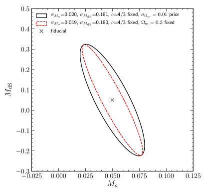
Figure 4: Joint 68% confidence contours for $M_{a}$ and $M_{\rm dS}$ with fixed $c=4/3$, with a prior of 0.01 on $\Omega_{m}$ (solid curve) or fixed $\Omega_{m}$ (dashed curve).

IV.2 Binned Gravity Constraints

To return to a more model independent approach to constraining gravity, we now estimate uncertainties of the $2\times 3$ bin values of $G_{m}$, i.e. looking for trends between low and high $k$ (larger and smaller scales) and from high to mid to low redshift. The parameter set is now $(G_{11},G_{12},G_{13},G_{21},G_{22},G_{23},\Omega_{m})$, and their fiducial values are the optimized fit values as described in Sec. III.

Table 2 compiles the results. At low $k$, the effect of the modified gravity on the observable $f\sigma_{8}$ is smaller than the precision of the data, and it is difficult to see any distinction from GR (i.e. $G_{m}=1$). For the $k_{\rm eff}=0.125$ bin, however, deviations from GR do start to have a noticeable effect. Note that since deviations in the low $a$ (high redshift) bin impact $f\sigma_{8}$ at all later redshifts, the precision on $G_{m}$ at low $a$ is tightest. At high $a$ (low redshift), the $G_{m}$ bin extending from $z=[0,0.5]$ only affects three data slices having reasonable precision: those at $z=0.25$, 0.35, 0.45, and so the uncertainties on $G_{m}$ at high $a$ become larger.

Bin of $G_{m}$	$G_{\rm bin}-1$	$\sigma(G_{\rm bin})$	$\sigma_{+}(G_{\rm bin})$
low $k$, low $a$ [11]	0.006	0.019	0.018
low $k$, mid $a$ [12]	0.031	0.104	0.103
low $k$, high $a$ [13]	0.052	0.377	0.137
high $k$, low $a$ [21]	0.029	0.018	0.018
high $k$, mid $a$ [22]	0.127	0.094	0.093
high $k$, high $a$ [23]	0.158	0.290	0.135

Table 2: Information matrix constraints on $G_{m}$ in each of the $2\times 3$ bins. Low/high $k$ refers to $k_{\rm eff}=0.055$, 0.125 respectively; low/mid/high $a$ refers to the ranges [0.37,0.5], [0.5,0.667], [0.667,0.833]. The $G_{\rm bin}-1$ column gives the fiducial value (i.e. the optimized values from Sec. III) and the last two columns shows the $1\sigma$ uncertainties in determining those values from the projected redshift space distortion data ($\sigma$ column), and also including a peculiar velocity measurement ($\sigma_{+}$ column; see Sec. IV.3).

The power to discriminate modifications from GR becomes greater when assessing the joint, rather than 1D, likelihood. Figure 5 shows the marginalized 2D joint confidence contours for all combinations of the $G_{\rm bin}$. Note that the parameters are fairly independent, with the greatest correlation coefficient being $-0.6$ between $G_{21}$ and $\Omega_{m}$; between the $G_{\rm bin}$ themselves, the maximum amplitude correlation is $-0.4$.

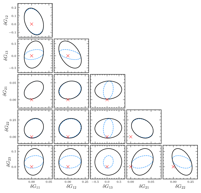
Figure 5: Corner plot showing 2D joint 68% CL constraints on the gravitational strength parameters in the two bins of $k$ and three bins of redshift. The red $\times$ denotes the GR value (0,0). The solid black contours use redshift space distortion data over $z=[0.2,1.7]$; the blue dashed contours add peculiar velocity data at $z=0.1$ (see Sec. IV.3). The matter density $\Omega_{m}$ is marginalized over with a prior of 0.01.

The red $\times$’s show the GR value in each panel, and we see that at low $k$ there is no statistically visible deviation from GR, even among the crosscorrelations (upper tip of the triangle). At high $k$ we see GR lies at or outside the 68% CL contour, and the deviation is especially noticeable in the crosscorrelations (right tip of the triangle). The overall difference in a GR fit to growth rate data from a cosmology with the fiducial modified gravity is $\Delta\chi^{2}=+20$, with 6 fewer parameters, giving at least a hint that one should look beyond GR. As in Sec. IV.1 we find that tightening the prior on $\Omega_{m}$ gives little improvement since there is not much covariance. Only a further generation of more precise data could improve the constraints on gravity in this model independent approach – or combination with other probes of growth.

IV.3 Impact of Low Redshift Data

Another method being implemented with current surveys, such as DESI, to measure directly the growth rate is peculiar velocities [40, 41]. This can improve the precision at low redshift dramatically over redshift space distortions, which are limited by low available volume for clustering statistics. We consider the addition of a single redshift measurement for $f\sigma_{8}$ at $z=0.1$ with precision 3% at each of $k_{\rm eff}=0.055$, 0.125 and investigate its impact on the gravitational constraints. This precision is a rough approximation of what DESI spectroscopy may provide from peculiar velocity measurements [40, 41]. (Note that in the future kinematic Sunyaev-Zel’dovich (kSZ) velocity measurements may also make precise growth rate constraints; see, e.g., [42, 43, 44, 45].)

This single redshift data point improves the constraints on the binned $G_{m}$ approach as shown by the last column in Table 2 for the 1D uncertainties and the dashed blue contours in Fig. 5 for the 2D joint constraints. Leverage is added particularly in the late time bin, i.e $G^{\rm bin}_{i3}$, such that GR is now pulled to the edge of many of the 2D joint confidence contours. The greatest effect is on $G_{13}$–$G_{23}$, where the uncertainty area is reduced by a factor 5.8. The total $\Delta\chi^{2}$ distinction from GR is now $\Delta\chi^{2}=28$, i.e. the one peculiar velocity data point distinguishes from GR by $\Delta\chi^{2}=8$.

For the scalar-tensor Padé approach we also find that the peculiar velocity data on the growth rate at $z=0.1$ can have good complementarity with the redshift space distortion measurements. While this one added data point does help to determine the amplitude parameter $c$, lowering $\sigma(c)$ from 1.7 without the $z=0.1$ data to 0.8 with, this is still not sufficient. Fixing $c=4/3$ as for $f(R)$ theories as discussed in Sec. IV.1, the peculiar velocity data has excellent leverage, as seen in Fig. 6. Now $\sigma(M_{a})=0.014$, down from 0.020, and $\sigma(M_{\rm dS})=0.094$, down from 0.181. The overall uncertainty area reduces by a factor 2 by adding the $z=0.1$ peculiar velocity measurement. Using the same naive procedure as before to estimate $f_{R0}$, the $1\sigma$ upper limit on $M_{a}+M_{\rm dS}$ is 0.19, for a lower limit on the fiducial model of $|f_{R0}|\gtrsim 2.9\times 10^{-6}$.

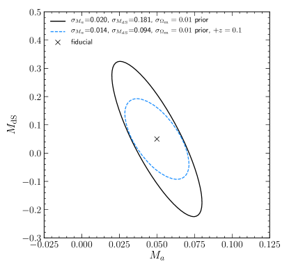
Figure 6: Joint 68% confidence contours for $M_{a}$ and $M_{\rm dS}$ with fixed $c=4/3$ and a prior of 0.01 on $\Omega_{m}$, for redshift space distortion only (solid curve, as in Fig. 4), and with the peculiar velocity data at $z=0.1$ (dashed blue curve).

V $2\times 2$ Bins

To get clearer distinction from GR we could use fewer bins in $a$, albeit at the loss of some evolutionary information on $G_{m}$. To explore this, we consider two bins in $a$ for $G_{m}$: $a=[0.25,0.556]$ and $a=[0.556,0.833]$, with the dividing line at $z=0.8$ so there will be sufficient precise data in both bins. The two bins in $k$ remain as is, with a piecewise constant form for the $G_{m}$ bin values. For just two bins in $a$, piecewise constant $G_{m}$ will not give a sufficiently accurate $\widehat{f\sigma_{8}}$ relative to the exact $f\sigma_{8}$, so we use a piecewise linear form, with continuity at the bin boundary $z=0.8$. (See Sec. III for a discussion of bins vs interpolated node values. In actual data analysis one might want to assess both.) We call our new $2\times 2$ gravity parameter set $G_{1A}$, $G_{1B}$, $G_{2A}$, $G_{2B}$, where the first index indicates low/high $k$ as before, and the second index $A/B$ indicates low/high $a$. (We change from numbers to letters to avoid confusion with the $G_{11}$ etc. from the $2\times 3$ set.) The bin values are defined at the midpoint in $a$ of each bin.

Figure 7 illustrates that the maximum deviation in reconstructing $f\sigma_{8}$ can be under 0.2% even with only two bins in $a$. As before we use bin centers at $k_{\rm eff}=0.055$, 0.125 and optimize the values of $\delta G^{\rm bin}$ to minimize the rms fractional deviation of $\widehat{f\sigma_{8}}$ from $f\sigma_{8}$ given by the fiducial scalar-tensor model. The optimized values are $\delta G_{1A}=0.011$, $\delta G_{1B}=0.048$, $\delta G_{2A}=0.049$, $\delta G_{2B}=0.15$.

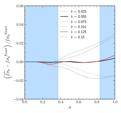
Figure 7: The fractional difference of $f\sigma_{8}$ using the optimized $2\times 2$ binned $G_{m}^{\rm bin}$ (giving $\widehat{f\sigma_{8}}$) vs using the exact modified gravity $G_{m}$ (giving $f\sigma_{8}^{\rm Exact}$) is plotted vs $a$ for various $k$. As in Fig. 3, only the values at $k_{\rm eff}=0.055$, 0.125 are observationally relevant. Similarly, the relevant (i.e. good data precision) range in $a$ is indicated by the unshaded region.

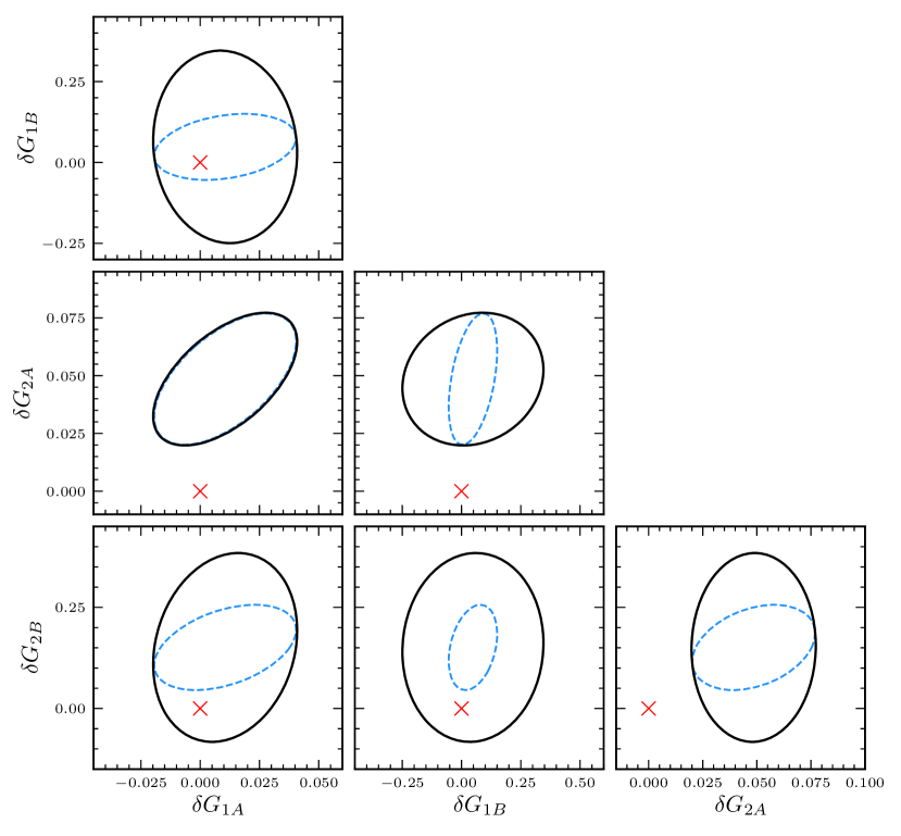
Figure 8: Corner plot showing 2D joint 68% CL constraints on the gravitational strength parameters in the two bins of $k$ and two bins of redshift. The red $\times$ denotes the GR value (0,0). The solid black contours use redshift space distortion data over $z=[0.2,1.7]$; the dashed blue contours add peculiar velocity data at $z=0.1$ (see Sec. IV.3). The matter density $\Omega_{m}$ is marginalized over with a prior of 0.01.

Therefore we can use the $2\times 2$ bin parametrization for robust comparison to projected data, and derive constraints on the gravity parameters. The corner plot of the 2D joint confidence contours is shown in Fig. 8. Now, several panels show GR as lying significantly outside the 68% confidence contour, either using redshift space distortion data alone or adding the peculiar velocity data at $z=0.1$. In some cases it lies outside the 95% joint confidence limit.

As before, the discrimination from GR is most statistically significant for the higher $k$ bin. The higher redshift bin also has tighter constraints than the lower redshift bin. The peculiar velocity data continues to exhibit strong leverage in complementarity with redshift space distortion measurements. In the $2\times 2$ case, the total distinction from GR is now $\Delta\chi^{2}=23$, for two fewer parameters than the $2\times 3$ case. This improves to $\Delta\chi^{2}=32$ with the peculiar velocity data point at $z=0.1$. The greatest improvement due to adding peculiar velocity data is on the $\delta G_{1B}-\delta G_{2B}$ joint contour, where the overall uncertainty area is reduced by a factor of 7.

VI Conclusions

The growth rate of cosmic structure is now being measured precisely by the current generation of spectroscopic surveys. This can combine with expansion history information to tighten constraints on dark energy and cosmic acceleration. However, beyond general relativity the growth rate carries extra information on the theory of gravitation, and for many theories this includes scale dependence even in the linear to quasilinear density regime.

We have demonstrated that the scale dependence in canonical scalar-tensor theories of gravity can be accurately accounted for by a model independent binning of the gravitational coupling: 2 bins in $k$ and 3 bins in $a$ deliver 0.02-0.27% rms accuracy in the full growth rate $f\sigma_{8}(k,a)$ even for a fairly conservative scalar-tensor gravity theory for comparison to observations. Such model independent bins have little covariance and are readily interpretable.

If one does not use all the physics present in scalar-tensor gravity, e.g. uses a power law in $a$ for $G_{m}$ rather than the true Padé form, or neglects the freezing of the scalaron mass as the universe is dominated by cosmic acceleration, we show that the results will be strongly different, both quantitatively and in interpretation. Some other models of gravity may contain a constant offset, i.e. constant deviation from GR even at low $k$, and these tend to be easier to constrain but address different physics.

Fitting parameters in the scalar-tensor form itself, thus being somewhat more model dependent, does not work due to strong covariances. Only when a particular class is chosen, such as $f(R)$ gravity, to fix the amplitude parameter $c$ can the shape parameters $M_{a}$, $M_{\rm dS}$ describing the scale dependence be fit with reasonable precision. These can be related to more specific quantities such as $|f_{R0}|$ and we demonstrate potential distinction from general relativity by obtaining a lower bound $|f_{R0}|\gtrsim 1.4\times 10^{-6}$ (in contrast to a spuriously tight $[0.8,1.2]\times 10^{-5}$ when ignoring the necessary de Sitter physics) for a model with true $|f_{R0}|\approx 10^{-5}$.

Of great promise is the strong complementarity of low redshift peculiar velocity probes of the growth rate with redshift space distortions from surveys at higher redshift. Recall that the growth rate at low redshift is sensitive to the cosmic gravitational history at all higher redshifts. Peculiar velocity data at $z\approx 0.1$ can tighten the 2D joint uncertainty area on binned gravity parameters by up to a factor 7, and raise the statistical significance of discrimination from general relativity to several measurements of 95% confidence level, or an overall $\Delta\chi^{2}=28$. While the precisions we adopted for RSD and peculiar velocity measurements are reasonable projections, it is quite exciting that DESI has already acquired substantial data and that actual analysis, including for various $k_{\rm max}$ and with neutrino mass, will be forthcoming in the next few years.

Finally, we also explore an alternate model independent parametrization with $2\times 2$ bins of $G_{m}$ and find it also works well. It accurately reproduces the full scalar-tensor prediction for $f\sigma_{8}(k_{\rm eff},a)$ with two fewer parameters. The constraints from projected data tighten, with greater discrimination power from GR. Two downsides are a more coarse grained view of the evolution in $a$, and a somewhat greater correlation between bins (because of the needed continuous piecewise linear rather than piecewise constant parametrization). One could envision using $2\times 2$ as an alert for a deviation from GR, and then reanalyzing the data with $2\times 3$ to pick up finer detail.