Dialogue Term Extraction using Transfer Learning and
Topological Data Analysis

Abstract

Goal oriented dialogue systems were originally designed as a natural language interface to a fixed data-set of entities that users might inquire about, further described by domain, slots and values. As we move towards adaptable dialogue systems where knowledge about domains, slots and values may change, there is an increasing need to automatically extract these terms from raw dialogues or related non-dialogue data on a large scale. In this paper, we take an important step in this direction by exploring different features that can enable systems to discover realizations of domains, slots and values in dialogues in a purely data-driven fashion. The features that we examine stem from word embeddings, language modelling features, as well as topological features of the word embedding space. To examine the utility of each feature set, we train a seed model based on the widely used MultiWOZ data-set. Then, we apply this model to a different corpus, the Schema-Guided Dialogue data-set. Our method outperforms the previously proposed approach that relies solely on word embeddings. We also demonstrate that each of the features is responsible for discovering different kinds of content. We believe our results warrant further research towards ontology induction, and continued harnessing of topological data analysis for dialogue and natural language processing research.

1 Introduction

Dialogue systems are becoming increasingly popular as natural language interfaces to complex services. Goal-oriented dialogue systems, which we see as the main area of application of the results presented here, are intended to be capable of conversing with a user to solve one or more tasks. They need to provide factual information and plan ahead over the course of multiple turns of dialogue. Thus, they differ fundamentally from chat-based dialogue systems, which aim to engage the user in interesting conversation by offering entertainment. Chat-based systems have been successfully trained using fully end-to-end approaches founded on large pretrained models Adiwardana et al. (2020); Lin et al. (2020); Zhang et al. (2020); Thoppilan et al. (2022). In contrast, state-of-the-art goal-oriented dialogue systems continue to rely on a pre-defined ontology: a database comprising domains (i.e., general topics for interaction), slots (constructs belonging to a particular topic), and values (concrete instantiations of such constructs) Ultes et al. (2017); Zhu et al. (2020); Kulhánek et al. (2021); Peng et al. (2021); Lee (2021); He et al. (2022).

Consequently, state-of-the-art goal-oriented dialogue systems still have a high reliance on manual labour. Firstly, the underlying ontology needs to be manually designed for each domain of conversation Milward and Beveridge (2003). Secondly, the dialogue system needs to learn from a certain amount of dialogue data labelled with concepts from that ontology in order to recognize and understand these concepts in context Young et al. (2013). This manual annotation is again challenging, time-consuming and expensive Budzianowski et al. (2018). There is thus a strong need for methods that can automate ontology construction from raw data. Moreover, ontology construction from raw dialogue data would have two-fold benefits: the dialogue data would be labelled automatically as the ontology is constructed, thus rendering any human involvement unnecessary.

In this work, we concentrate exclusively on the first step of ontology construction: term extraction. The terms relate to regions of importance in the raw text. The subsequent steps of ontology construction, which we do not consider here, usually involve some form of clustering to boil down the extracted terms to a smaller number of concepts before they are finally organized into a full ontology.

Traditionally, term extraction begins by extracting terms based on frequency, in a way that aims to maximize recall Nakagawa and Mori (2002); Wermter and Hahn (2006). As frequency alone is a fairly primitive feature, this first step has close to zero precision and typically results in far too many terms. This makes further substantial filtering necessary within the term extraction step Frantzi and Ananiadou (1999). Filtering typically relies on heuristics or pre-existing natural language processing (NLP) models that have been trained on unrelated data, e.g., semantic parsers Bourigault and Jacquemin (1999); Aubin and Hamon (2006). Heuristics as well as NLP models require substantial amounts of linguistic expertise to be created.

In this work, we take a purely data-driven approach toward dialogue term detection to circumvent these limitations. The high dimensional data spaces arising from word embeddings are hard to understand and visualize. Topological data analysis (TDA) is a collection of mathematical tools which provides measurements of the geometry of high-dimensional point clouds at various scales. The major advantage of topological features is their invariance under small deformations and rotations, as opposed to the coordinates of the embedding vectors. This leads to characteristics that are very generalizable and not dependent on the exact data set used for training. The utility of TDA for NLP and dialogue modelling in particular are still under-explored. We believe that information that can be gathered using topological methods has considerable predictive power concerning term extraction, which to the best of our knowledge we exploit with this work for the very first time.

Starting from the approach of Qiu et al. (2022), we train a BIO-tagging Ramshaw and Marcus (1995) model on the widely used MultiWOZ Budzianowski et al. (2018) data-set as the seed set by fine-tuning general purpose large pre-trained language models. Our BIO-tagger accepts various features as input, all of which uniquely contribute to solving the task. We measure the zero-shot transfer ability of our proposed models on the Schema-Guided Dialogue Rastogi et al. (2020) data-set, another well-established large-scale corpus for dialogue modelling. Our contributions are as follows:

• We present novel features to solve the term extraction task. Our experimental results show significant improvements over a strong baseline, a recently proposed model that only takes contextual word embeddings as input.

• We demonstrate the suitability of masked language modelling scores to predict relevant terms.

• We exhibit the suitability of a range of topological features of neighbourhoods of word vectors to predict terms of relevance, including terms that are not present in the original seed training set.

• We make our code publicly available.

Our proposed method for term extraction leverages semantics as well as information gained from topological data analysis. No element of our approach requires linguistic knowledge, nor do we rely on any heuristics. Our models are either trained from scratch using a seed data-set, or leverage the predictive power of pre-trained and then fine-tuned large general purpose language models. These models learn via self-supervision on large corpora, and our additional training only requires a moderate amount of labelled seed data.

2 Related Work

It is normally assumed that the ontology is provided and built independently of the dialogue system. For instance, in information seeking dialogue systems, this would be a structured representation of the database. Approaches to ontology learning from texts generally involve enriching a small ontology with new concepts and new relationships using text mining methods such as linguistic techniques and lexico-syntactic patterns Pantel and Pennacchiotti (2006); Aguado De Cea et al. (2008), clustering techniques Agirre et al. (2000); Witschel (2005), statistical techniques Sugiura et al. (2003) and association rules Bodenreider et al. (2005); Gulla et al. (2009). The majority of these methods require some form of human intervention. The potential of machine learning in this area has been demonstrated in the Never-Ending Language Learning (NELL) project Mitchell et al. (2018). NELL learns factual knowledge from years of self-supervised experience in harvesting the web, using previously learned knowledge to improve subsequent learning.

In the pipeline of knowledge base construction, term extraction is typically the first step. One example of a term extractor is presented in Sclano and Velardi (2007). It uses a part-of-speech (POS) tagger to select nouns, verbs and adjectives to which a number of heuristic frequency-based probabilistic models are applied to select term candidates. WordNet Fellbaum (1998) is employed to handle misspellings. A number of more recent methods for knowledge base construction start with a similar approach as Sclano and Velardi (2007). In Romero and Razniewski (2020) we can also see heavy reliance on frequency, the use of dependency parsers in Nguyen et al. (2021), as well as rules based on lexical and numerical features and the use of WordNet as in Chu et al. (2019).

A notable example of dialogue ontology induction is presented in Hudeček et al. (2021), where a rule-based semantic parser is used as a starting point to propose an initial set of concepts. A more data-driven approach is presented by Qiu et al. (2022) who proposed training a BIO-tagger on fine-tuned contextual embeddings to induce slots. The approach is validated on MultiWOZ via leave-one-out domain experiments. We take this work as a starting point. In very recent work, Yu et al. (2022) propose ontology induction using language modelling attention maps and regularized probabilistic context free grammar to detect regions of interest in text, followed by clustering. This work is complementary to ours, and it would be interesting to explore its combination with our proposal.

The ‘Beyond domain APIs’ track of the 9th dialog system technology challenge (DSTC9) Gunasekara et al. (2020) aimed to remove friction in task-oriented dialogue systems where users might issue a request that is out of a system’s scope. While DSTC9 aimed to integrate non-dialogue data into dialogue, none of the challenge submissions attempted ontology construction or expansion.

Topological data analysis remains largely underutilized in natural language processing. One notable exception is the work presented by Jakubowski et al. (2020). It shows that the Wasserstein norm of degree zero persistence of punctured neighbourhoods in a static word embedding correlates with the polysemy of a word. Tymochko et al. (2021) apply persistent homology to word embedding point clouds with the goal of distinguishing fraudulent from genuine scientific publications. Their best performing model utilizes persistence features derived from time-delay embeddings of term frequency data. Kushnareva et al. (2021) compute persistent homology of a filtered graph constructed from the attention maps of a pre-trained language model and harness the features for an artificial text detection task.

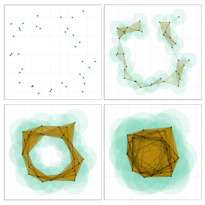
Figure 1: Illustration of the Vietoris-Rips complex $\operatorname{VR}_{\varepsilon}$ for four different values of $\varepsilon$.

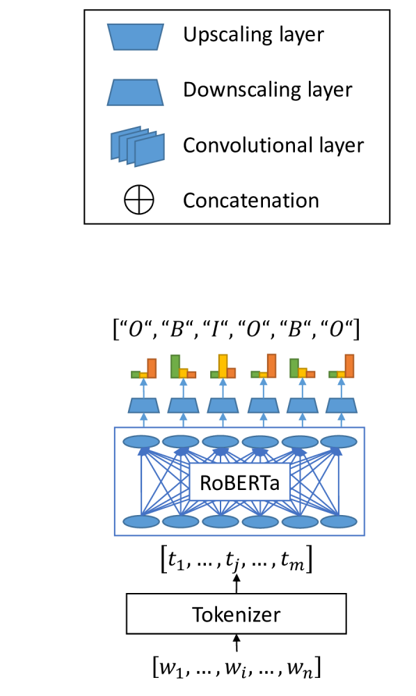
(a) Baseline model (subsection 4.1)

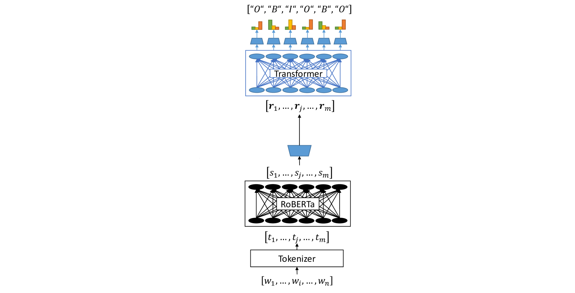
(b) MLM model (subsection 4.2)

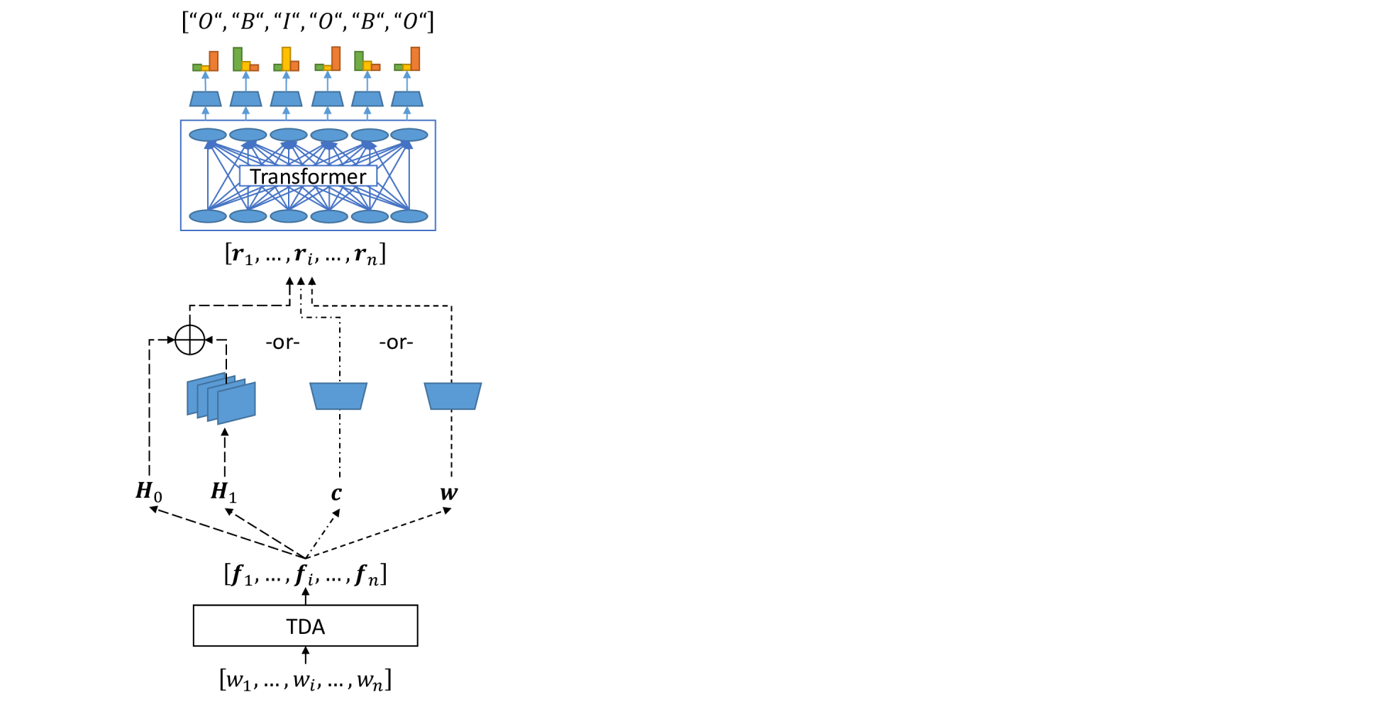
(c) TDA models (subsection 4.3)

Figure 2: Our three main architectures for dialogue term detection. Their main distinction is the type of features expected as input. Blue denotes trainable model components. For illustration purposes, here $n=6$.

3 Background on TDA

Topological data analysis (TDA) is an emerging toolkit of mathematical methods for analysing the ‘shape’ of data. In our case, we study point clouds resulting from word vector embeddings, but these general methods apply equally well to spaces of sensor data, images, or audio. Topology measures important features of a geometric space which are invariant under certain structure preserving transformations such as scaling, rotation, stretching and bending. Homology quantifies the presence or absence of $d$-dimensional holes in a geometric space: In dimension $d=0$ the homology group $H_{0}$ computes the connected components of a space, while in dimension $d=1$ the group $H_{1}$ describes the non-fillable closed loops in the space.

Consider a discrete point cloud $P\subset\mathbb{R}^{M}$ equipped with a distance such as the Euclidean metric or the cosine distance. To apply topological tools to $P$, we need to turn $P$ into a geometric space. One such ‘geometrization’ is the Vietoris-Rips complex $\operatorname{VR}_{\varepsilon}$, which produces, for each non-negative filtration parameter $\varepsilon$, a simplicial complex, a certain higher-dimensional generalization of a graph. To construct $\operatorname{VR}_{\varepsilon}$, we consider a collection of higher-dimensional balls of radius $\varepsilon$ centred at the data points. As $\varepsilon$ increases, the balls grow and merge as in Figure 1. Their overlaps determine the vertices, edges, triangles and higher-dimensional pieces of the complex $\operatorname{VR}_{\varepsilon}$.

The motivation for varying $\varepsilon$ is to measure the ‘scale’ or ‘resolution’ of different topological features. The filtration parameters $\varepsilon$ at which different $k$-dimensional holes appear and disappear in $\operatorname{VR}_{\varepsilon}$ are summarized in a multiset of points in the plane, visually represented as a persistence diagram as in Figure 4. Each dot in the diagram corresponds to a feature. Its horizontal coordinate is the birth time, its vertical coordinate the death time of the feature. The farther a dot is away from the diagonal, the longer the corresponding feature persists across the range of the parameter $\varepsilon$, and thus the more likely it is to reflect a large-scale topological property of the point cloud $P$. For an overview of persistent homology from a computational perspective, see Edelsbrunner and Harer (2010).

4 Dialogue Term Detection

4.1 Term Tagging

Our ultimate goal is to extract terms describing domains, slots and values from raw dialogues. In order to achieve this, we adopt the BIO-tagging mechanism presented by Qiu et al. (2022). In the seed corpus, the spans where concepts occur are tagged with labels ‘B’ (beginning of concept), ‘I’ (inside of concept) and ‘O’ (outside of concept), without distinguishing between different concepts. The baseline model is trained on RoBERTa Liu et al. (2019) embeddings as features, and shows modest generalization capabilities when tested in leave-one-out domain experiments.

We investigate two fundamentally different feature sets to increase the generalization capability of models fine-tuned for BIO-tagging. For each feature, we use a specific input projection and train a transformer followed by a token-level classification head. This architecture is illustrated in Figure 2. As the models extract different terms depending on the feature type they are trained on, we use the union of the predictions of all the TDA models, respectively, of all the models, to obtain the final set of terms. One may also build a combined model using all features as joint input, however due to the nature of the training this would maximize accuracy and not recall.

4.2 MLM Model

The first feature set we consider stems from context-level information captured by large pretrained masked language models (MLM) like BERT Devlin et al. (2019) and RoBERTa. Our hypothesis is that, based on how confident an MLM is in predicting a certain word, we can infer the meaningfulness of said word. We introduce the masked language modelling score (MLM score) $s(w_{i})=1-p_{\textrm{MLM}}(w_{i}\mid[w_{1},\dots,w_{i-1},\textrm{MASK},w_{i+1},\dots,w_{n}])$ as the probability that the word $w_{i}$ is not predicted by the MLM for the MASK token on position $i$, based on the context $[w_{1},\dots,w_{i-1},\textrm{MASK},w_{i+1},\dots,w_{n}]$. Thus, meaningful words should have a high MLM score, as illustrated in Appendix C. The total MLM score $s_{w_{i}}$ of a word is the average of all scores of all appearances of the word in the data-set.

4.3 TDA Models

Topological features allow us to address the following problem observed in transfer learning: Tagging models trained directly on the word embedding vectors derived from one dialogue data-set do not generalize well to the embeddings of a different data-set. We propose the investigation of topological features of neighbourhoods of word vectors. Such topological features capture geometric properties that are invariant under distance-preserving transformations of the data points, and are more generalizable and stable under perturbation than the word-vectors and language model features themselves. Our hypothesis is that these features reflect properties of words that are data-set independent.

The simplest topological feature we examine is a codensity vector that measures the data density in neighbourhoods of various sizes of a given word vector. A second, far more sophisticated feature that we utilize is persistence. As explained in section 3, persistence detects geometric features of a data-set at different scales. While degree zero persistence is closely related to density measures, higher degree persistence captures more refined information. Finally, we also investigate the Wasserstein norm as a two-dimensional summary of persistence. We now describe these topological descriptors with more mathematical rigour.

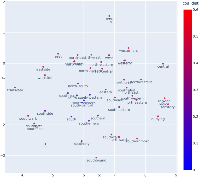
Figure 3: 2-dim. t-SNE projection of the neighbourhood $\mathcal{N}_{50}(w)$ of $w=\text{`south'}$. Colours indicate cosine distance from $w$ in the original $384$-dim. embedding space.

Word embedding neighbourhoods

Our topological tagging models use descriptors derived from neighbourhoods of words in the embedding space. The neighbourhoods are defined relative to a point cloud $X\subset\mathbb{R}^{M}$ constructed from the word vectors of an ambient vocabulary embedding. For a given centre $w\in\mathbb{R}^{M}$, let $\mathcal{N}_{n}(w)\subset X\cup\{w\}$ denote the subset of the $n$ nearest neighbours of $w$ with respect to cosine distance (including $w$ itself). In our experiments, we employ neighbourhoods of size $n=50$. See Figure 3 or Appendix A for examples.

The ambient point cloud $X$ in the embedding space needs to be independent of the specific dialogue vocabulary, so that the resulting persistence features of the neighbourhoods remain comparable. Our vocabulary consists of the 50,000 most common words in the English language, extracted from Grave et al. (2018). The embeddings for the point cloud $X$ are created from the SentenceTransformers Reimers and Gurevych (2019) paraphrase-MiniLM-L6-v2 model. These dense embeddings of dimension $M=384$ can be meaningfully compared with cosine similarity. Note that even though we are using a contextualized model for creating the embeddings, we obtain a ‘static’ point cloud $X$ containing the 50,000 vocabulary vectors. For building the neighbourhood $\mathcal{N}_{n}(w)$ of a word $w$ not contained in the ambient vocabulary $X$, we first produce $w$’s SentenceTransformers embedding.

Codensity

The $k$-codensity in a point $w$ of a point cloud $P\subset\mathbb{R}^{M}$ is defined as the distance from $w$ to the $k$th nearest point in $P$. Thus, points with many neighbours at a close distance have a small codensity, which corresponds to a large density of the point cloud around the point $w$. We construct a 6-dimensional vector $c$ containing the $k$-codensity of $\mathcal{N}_{50}(w)$ at $w$ for $k\in\{1,2,5,10,20,40\}$, with the intention of quantifying the neighbourhood density at various scales.

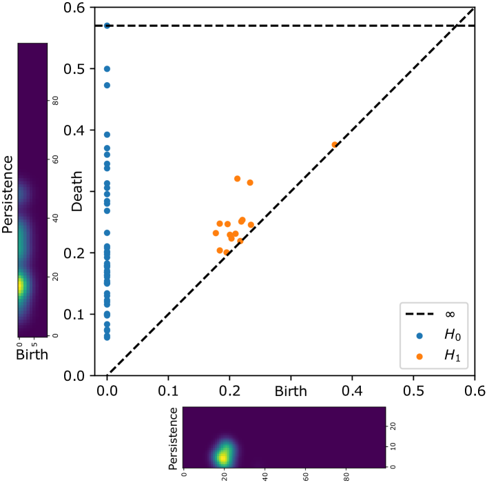
Figure 4: Persistence diagram of $\mathcal{N}_{50}(w=\text{`south'})$ for $H_{0}$ (blue dots) and $H_{1}$ (orange dots) and corresponding persistence images (left: $H_{0}$, bottom: $H_{1}$).

Persistence

We produce the persistence diagram (PD) of the sub-point-cloud $\mathcal{N}_{n=50}(w)\subset\mathbb{R}^{384}$ with filtration parameter in the range $[0,1]$ using cosine distances. Practically, we apply Ripser Bauer (2021) and its Python interface Tralie et al. (2018) for computations of $H_{0}$ and $H_{1}$ with $\mathbb{F}_{2}$-coefficients. We restrict to 0- and 1-dimensional homology to keep the computational costs reasonable. The resulting persistence diagram is a multiset of points in the unit square $[0,1]^{2}$, as in Figure 4.

Before we can pass the persistence diagrams into the tagging model, we have to apply a vectorization step, i.e., map the persistence diagrams into a space which is suitable for training machine learning classifiers. For this we use persistence images Adams et al. (2017), a short overview of the construction and our choice of parameters is given in Appendix B. Figure 4 contains an example of the persistence images for the ‘south’ neighbourhood.

Wasserstein norm

The Wasserstein distance is a commonly applied measure of similarity of persistence diagrams Cohen-Steiner et al. (2010). In our case, it is a rough numerical estimate of the similarity of the shapes of neighbourhoods. The Wasserstein norm $\left\lVert D\right\rVert$ is the Wasserstein distance from $D$ to the empty diagram. For constructing the input features of the Wasserstein models, we compute the order-$1$ Wasserstein distances with Euclidean ground metric using the GUDHI library The GUDHI Project (2022) separately for the $H_{0}$ and $H_{1}$ persistence diagrams, leading to a 2-dimensional Wasserstein input vector $\omega$.

4.4 Training & Inference

The MLM score model (2(b)) and the TDA models (2(c)) use the following input projections of the respective input features: The $100$-dimensional $H_{0}$ persistence image vector and $30\times 100$-dimensional $H_{1}$ persistence image are passed into the model independently and concatenated after downscaling $H_{1}$ to dimension $396$ via a convolutional layer with kernel size $35\times 25$. Then they are input to a transformer with hidden dimension $h=496$ and $8$ attention heads. The transformer output is the input for a token-level classification head after passing through a dropout layer.
The $6$-dimensional codensity vector $c$, the $2$-dimensional Wasserstein norm vector $\omega$ and the single-dimensional MLM score $s$ are all upscaled to hidden dimension $h=128$ via a 2-layer fully connected neural network to expand the representation space, before being put into three separate transformers with hidden dimension $h=128$ and $16$ attention heads. The transformer sequence output passes through a dropout layer into the token-level classification head. The token-level classification head consists of a dropout layer, a feed-forward layer with hidden dimension $h$, another dropout, $\tanh$ for activation and an output projection to dimension $3$ corresponding to the three possible BIO tags. The classification head is based on the implementation in the HuggingFace library Wolf et al. (2019), where the dropout rate for all layers is $0.1$.

We utilize RoBERTa encoders in two of our models (see Figure 2), once to obtain MLM scores with fixed parameters, and once to obtain contextual semantic embeddings after fine-tuning on the BIO-tagging task. We train each model on MultiWOZ with cross-entropy loss and a learning rate of $4\mathrm{e}{-5}$ using the AdamW optimizer Loshchilov and Hutter (2019), warm-up for $10\%$ of total training steps and linear decay afterwards. We train for 15 epochs, with training stopping early if the loss on the validation set stays within a range of $\delta=0.005$ and batch size 128 on one NVIDIA Tesla T4 GPU. For the much smaller training data in the leave-one-out experiments, the batch size is decreased to 32.

5 Experiments

We conducted experiments to answer the following questions: (1) Is it possible to train a model on the seed data-set that achieves a high recall rate on the unseen ontology? (2) Which of the proposed features is most valuable for that purpose? (3) What kind of concepts is the model able to find?

Note that we are mainly focusing on recall as evaluation measure, while retaining the F1-score of the baseline model. Improvements in precision can be achieved with further post-processing, such as clustering Qiu et al. (2022); Yu et al. (2022).

5.1 Data-sets

We use two well-established data-sets for modelling task-oriented dialogues. MultiWOZ Budzianowski et al. (2018); Eric et al. (2020) is a corpus of human-to-human dialogues that were collected in a Wizard-of-Oz fashion. Each conversation has one or more goals that revolve around seeking information about or booking tourism-related entities. The data-set consists of over 10,000 dialogues covering 6 domains. There are 30 unique domain-slot pairs that take approximately 4,500 unique values. Value occurrences are annotated with span labels. MultiWOZ is the seed set for training all of our term extraction models.

The Schema-Guided Dialogue (SGD) data-set Rastogi et al. (2020) is considerably larger than MultiWOZ, with dialogues spanning across 20 domains that represent a wide variety of services. The number of unique values is almost four times larger than in MultiWOZ. This means that any model trained on the significantly more narrow MultiWOZ seed data would need to be able to generalize extremely well to achieve reasonable term extraction performance on SGD. Therefore, SGD is an ideal data-set for our zero-shot experiments.

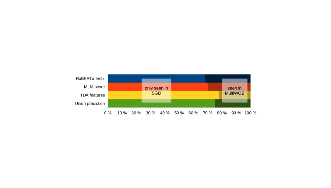
Figure 5: Percentage of extracted terms which were already seen during training or are only seen on SGD during test time.

5.2 Set-up

In order to investigate the models’ ability to extract terms in an unseen domain, we design two experiments. First, we conduct a leave-one-out domain experiment on MultiWOZ, similar to the approach taken by Qiu et al. (2022), with two important differences. We focus mainly on recall as the adequate evaluation measure for term extraction, and we do not allow partial matches of the tagged term. When designing the matching function, we were guided by the tolerance threshold of a picklist-based dialogue state tracker. For example, the term extractor is allowed to match ‘an expensive’ with the golden term ‘expensive’, as having a non-content word in the term would make no difference to the tracker. However, matching ‘Pizza Hut’ with the golden term ‘Pizza Hut Cherry Hinton’ is considered a false positive, as ‘Pizza Hut’ would not be precise enough for the tracker to distinguish entities. Note that such matches were considered by Qiu et al. (2022) as true positives, so our matching function is stricter. For both training and testing we limit ourselves to user utterances, as the system utterances may contain API calls, which is already structured data.

For the second experiment, we train our models on the training portion of the MultiWOZ data-set and test it on the SGD data-set. We then examine the overlap in true positives between models using different features. We also analyse the models’ abilities to extract terms referring to different domains and slots, highlighting easy and difficult terms.

5.3 Results

Leave-one-out domain

Approach	Measure	Taxi	Rest.	Hotel	Attr.	Train
RoBERTa	F1	0.87	0.81	0.68	0.91	0.84
embeddings	Recall	0.87	0.89	0.95	0.94	0.92
	Precision	0.87	0.76	0.53	0.89	0.77
MLM	F1	0.44	0.47	0.32	0.42	0.57
score	Recall	0.43	0.48	0.69	0.53	0.72
	Precision	0.46	0.46	0.21	0.35	0.47
Persistence	F1	0.72	0.61	0.41	0.63	0.65
image	Recall	0.79	0.69	0.87	0.65	0.92
vectors	Precision	0.67	0.54	0.27	0.61	0.50
	F1	0.57	0.46	0.38	0.51	0.62
Codensity	Recall	0.51	0.48	0.64	0.59	0.76
	Precision	0.64	0.44	0.27	0.45	0.52
Wasserstein	F1	0.57	0.50	0.45	0.46	0.48
norm	Recall	0.58	0.53	0.46	0.51	0.69
	Precision	0.57	0.47	0.45	0.43	0.37
TDA	F1	0.65	0.53	0.33	0.52	0.47
features	Recall	0.84	0.81	0.89	0.84	0.94
	Precision	0.53	0.39	0.20	0.37	0.31
Union	F1	0.65	0.53	0.26	0.49	0.44
prediction	Recall	0.95	0.92	0.97	0.98	0.98
	Precision	0.50	0.37	0.15	0.33	0.28

Table 1: Leave-one-out results on MultiWOZ.

We remove one of the five MultiWOZ domains in training and only test on it, so the model has not seen any dialogues in the left-out domain. We only utilize single domain dialogues in the training and test set. Results in Table 1 show that the recall increases for each unseen domain experiment when adding the predictions by the models trained on persistence and language modelling features to form the union prediction.

Unseen ontology

Approach	F1 $\uparrow$	Rec. $\uparrow$	Prec. $\uparrow$	L2 $\downarrow$	Tags
RoBERTa emb.	0.45	0.35	0.63	0.29	2757
MLM score	0.34	0.34	0.35	0.35	4933
PI vectors	0.47	0.46	0.48	0.20	4775
Codensity	0.37	0.34	0.42	0.52	4054
Wasserst. n.	0.42	0.40	0.44	0.62	4536
TDA features	0.48	0.63	0.39	-	8189
Union pred.	0.48	0.74	0.36	-	10398

Table 2: Dialogue term extraction results on SGD with models trained on MultiWOZ together with the total number of tagged terms per model. There are 5008 target terms in SGD. L2-norm is used as uncertainty measure for the single models.

The results in Table 2 show that adding the predictions of the new feature models improve both recall and F1-score significantly for term extraction on the unseen SGD ontology compared to the language model only baseline, without the need to fine-tune the embeddings on the token classification task with any SGD data. In Figure 5 the percentage of completely new terms found in the predictions of each model is shown. The TDA feature model predictions contain mostly unseen terms. Confidence scores would be critical in a subsequent automatic ontology construction. We compare the L2-norm of the model’s predictions to the ground truth label, showing that the model trained on persistence image vectors from MultiWOZ has the highest confidence score on the unseen SGD data.

Seen in MultiWOZ	Only seen in SGD	False negatives	False positives
Lebanese; Hotel Indigo London-Paddington; LAX International Airport; The Queen’s Gate Hotel; Hair salon	Delta Aesthetics; McDonald’s; 3455 Homestead Road; receiver; Pescatore	Little Hong Kong; Yankees vs. Rangers; Dr. Eugene H. Burton III; 341 7th street; La Quinta Inn by Wyndham Dacramento Downtown	Especillay by; Bears vs; Angeles and; Polk Street; theater please; resrevation; neaarby

Table 3: Example predictions of the Union model on SGD (typos are reproduced as they appear in the data-set). Examples for each of our other models can be found in Appendix E.

	i ’ d like to find a steakhouse that ’ s not very costly to eat at .
RoBERTa embeddings	i ’ d like to find a steakhouse that ’ s not very costly to eat at .
MLM score	i ’ d like to find a steakhouse that ’ s not very costly to eat at .
TDA features	i ’ d like to find a steakhouse that ’ s not very costly to eat at .

Table 4: Example of a normalized, tokenized utterance together with terms extracted by the different models. Unconnected boxes indicate separate terms, i.e., here the MLM score model assigned a B tag to ’steakhouse’ and a B tag to ’that’. More example utterances can be found in Appendix E.

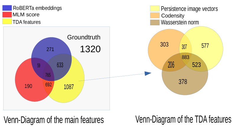
Figure 6: Venn-Diagram of SGD terms found in each of the three models using RoBERTa, MLM score, TDA features, as well as analysis of term overlap of the models trained on different TDA features.

Overlap

Figure 6 shows that the sets of extracted terms differ significantly by model. Therefore, the union of predictions is useful for capturing as many relevant terms as possible. The MLM score model already adds more terms to the fine-tuned language model. The topological features, however, by far supply the biggest portion of new terms. Among the different TDA features, the persistence images yield the largest number of additional terms.

Domain and slot coverage

Figure 7 demonstrates that the different models find various amounts of terms depending on the domain. The recall of the TDA models is the highest across all domains, while RoBERTa is only able to outperform the MLM score model in terms of recall in 5 out of 20 domains, e.g., in ‘music’ and ‘restaurants’, which contain many multi-word terms.

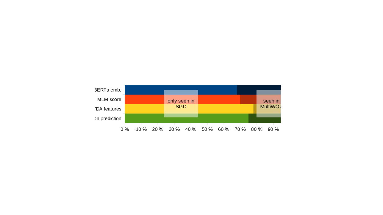
Figure 7: Recall per domain on SGD by our models compared with the baseline fine-tuned RoBERTa model.

Examples

False negatives tend to be long multi-word terms, as exemplified in Table 3. False positives predominantly include typos and incomplete terms. Predictions by RoBERTa contain $2.0$ words on average. In contrast, the MLM score model and TDA feature model term predictions have an average length of $1.6$ and $1.8$ words, respectively. We give an illustrative instance of terms extracted by the different models from an example utterance in Table 4.

6 Discussion and Future Outlook

Our novel term extraction approach based on topological data analysis and masked language modelling scores significantly outperforms the word-embedding-based baseline on the recall rate both in leave-one-out experiments and when applied to a completely different corpus. Importantly, our results demonstrate a strong ability of topological data analysis to extract domain independent features that can be used to analyse unseen data-sets. This finding warrants further investigation.

Our approach still produces a significant number of false positives. The next step in the ontology construction pipeline, clustering, could be deployed to significantly reduce that number, as has already been demonstrated by Yu et al. (2022). We believe that their approach and our approach could be combined, but that goes beyond the scope of this work.

However, ultimately, precision is only of secondary importance. In a typical goal oriented system, we have a dialogue state tracker tracking concepts through conversation. Whether or not the tracker is tracking some irrelevant terms does not impact the overall performance of a dialogue system. All that matters is that the tracker does track every term that actually is a concept. Of course, the computational complexity of the tracker increases linearly with the number of tracked terms Heck et al. (2020); van Niekerk et al. (2020); Lee et al. (2021). But, as can be seen from Table 2, our method merely doubles the number of terms, so the computational price tag is low. With this in mind, it is also conceivable that the tracker itself could be utilized to increase the precision. This would be an interesting direction for further research.

Some simpler options for improvement are more immediate: Here, we utilize SentenceTransformers only to provide static embeddings for each word, but of course a similar analysis can be applied to contextualized word embeddings, at the expense of higher computational complexity. Further, persistence images (subsection 4.3) could be replaced by features tailored to downstream tasks, such as features obtained from the novel Persformer model Reinauer et al. (2021).

7 Conclusion

To the best of our knowledge, we present the first application of topological features in dialogue term extraction. Our results show that these features distinguish content from non-content words, in a way that can be generalized from a training domain to unseen domains. We believe that these findings are only the tip of the iceberg, and warrant further investigation of topological features in NLP in general. In addition, we have shown that masked language modelling scores are useful for term extraction as well. In combination, the features we investigate allow us to make a significant step towards automatic ontology construction from raw data.

Appendix A Neighbourhoods and Persistence Diagrams

We produce a table with various figures of neighbourhoods, their persistence diagrams, Wasserstein norm vectors and codensity vectors in Figure 8.

	Neighbourhood	Persistence Diagram	Wasserst. / Codens.
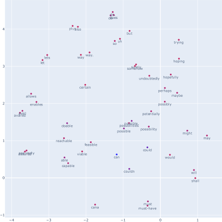
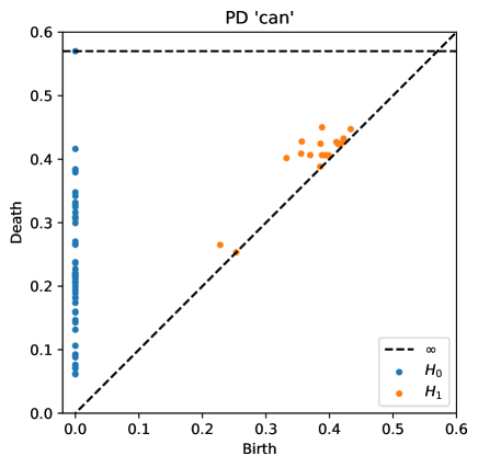
can			$\begin{pmatrix}7.712\\ 0.311\end{pmatrix}$ $\begin{pmatrix}0.181\\ 0.259\\ 0.307\\ 0.379\\ 0.402\\ 0.439\end{pmatrix}$
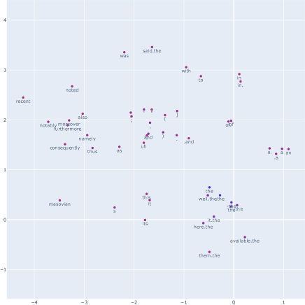
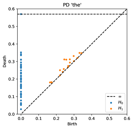
the			$\begin{pmatrix}6.490\\ 0.219\end{pmatrix}$ $\begin{pmatrix}0.099\\ 0.129\\ 0.213\\ 0.275\\ 0.318\\ 0.349\end{pmatrix}$
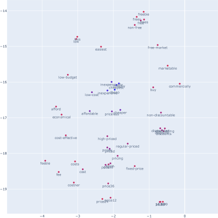
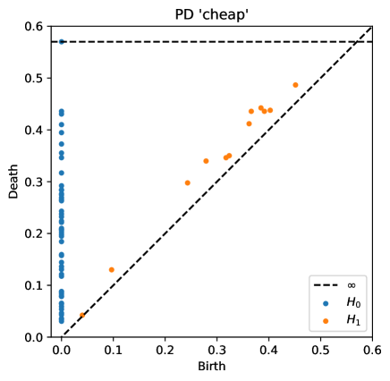
cheap			$\begin{pmatrix}6.823\\ 0.350\end{pmatrix}$ $\begin{pmatrix}0.059\\ 0.065\\ 0.195\\ 0.322\\ 0.387\\ 0.464\end{pmatrix}$
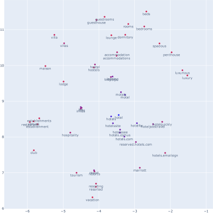
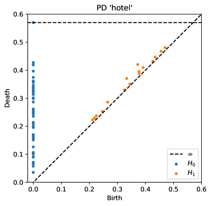
hotel			$\begin{pmatrix}7.902\\ 0.166\end{pmatrix}$ $\begin{pmatrix}0.106\\ 0.167\\ 0.217\\ 0.265\\ 0.374\\ 0.473\end{pmatrix}$

Figure 8: 2-dimensional t-SNE projection of the neighbourhood $\mathcal{N}_{50}(w)$; corresponding Persistence diagram; 2-dim. Wasserstein norm vector (for $H_{0}$ and $H_{1}$); 6-dim. codensity vector (for $k\in\{1,2,5,10,20,40\}$).

Appendix B Details about the Persistence Diagram Vectorization Step

We used the scikit-tda/persim library Saul and Tralie (2019) in the practical implementation of persistence images.

As a first step, the $(\textrm{birth},\textrm{death})$ coordinates of the dots in the persistence diagram are transformed into $(\textrm{birth},\textrm{lifetime}=\textrm{death}-\textrm{birth})$ coordinates. We then place a Gaussian kernel with variance $\sigma=0.0007$ onto each point in the $(\textrm{birth},\textrm{lifetime})$ diagram, linearly weighted by the lifetime. We sum up the various probability distributions and then integrate the resulting function over the patches of a rasterization with a pixel size of $0.1$ of the image plane. Adams et al. (2017) discuss that the performance of the resulting persistence images for downstream tasks is robust in the choices of these parameters. As usual in the Vietoris-Rips filtration, the birth of all the 0-dimensional homology classes in $H_{0}$ occur for radius $\varepsilon=0$, and we consider the persistence features in the range $[0.0,1.0]$. Thus, we only pass the 0th column of the generated $H_{0}$ persistence image to the model, which is a $100$-dimensional vector. For the $H_{1}$ persistence image, we take the entire birth range $[0.0,1.0]$ and persistence range $[0.0,0.3]$ into account, so that the image has dimensions $100\times 30$.

Appendix C Masked Language Modelling Score Examples

In Table 5 the MLM scores on MultiWOZ and SGD of example words show that the score is high for meaningful words across data-sets.

Word	Score on MultiWOZ	Score on SGD
cheap	0.96	0.92
restaurant	0.86	0.86
the	0.59	0.63
how	0.70	0.67
not	0.45	0.50

Table 5: Masked language modelling score examples.

Appendix D Further Experimental Results

See Table 6, Table 7, Table 8 and Table 9 for further experimental results.

	MultiWOZ				SGD
Approach	F1-Score	Recall	Precision		F1-Score	Recall	Precision
RoBERTa embeddings	0.80	0.91	0.72		0.45	0.35	0.63
MLM scores	0.38	0.83	0.25		0.34	0.34	0.35
Persistence image vectors	0.53	0.87	0.38		0.47	0.46	0.48
Codensity	0.42	0.76	0.29		0.37	0.34	0.42
Wasserstein norm	0.37	0.65	0.26		0.42	0.40	0.44
TDA features together	0.33	0.89	0.20		0.48	0.63	0.39
Union prediction	0.28	0.96	0.17		0.48	0.74	0.36

Table 6: Results of all models trained on MultiWOZ and tested on MultiWOZ and SGD.

Approach	MultiWOZ	SGD
RoBERTa embeddings	816	2757
MLM score	2174	4933
Persistence image vectors	1464	4775
Codensity	1658	4054
Wasserstein norm	1631	4536
TDA features	2867	8189
Union prediction	3712	10398

Table 7: Total number of terms tagged on MultiWOZ and SGD broken down per model trained on MultiWOZ. For reference, there are 645 target terms in total in MultiWOZ and 5008 in SGD.

	MultiWOZ				SGD
Approach	F1-Score	Recall	Precision		F1-Score	Recall	Precision
RoBERTa embeddings	0.65	0.92	0.50		0.83	0.88	0.78
MLM scores	0.32	0.76	0.21		0.37	0.33	0.44
Persistence image vectors	0.45	0.84	0.31		0.76	0.80	0.73
Codensity	0.37	0.69	0.25		0.50	0.49	0.51
Wasserstein norm	0.40	0.78	0.27		0.53	0.54	0.52
TDA features together	0.30	0.92	0.18		0.64	0.88	0.50
Union prediction	0.23	0.98	0.13		0.61	0.98	0.44

Table 8: Results of all models trained on SGD and tested on MultiWOZ and SGD.

Approach	F1-Score	Recall	Precision
RoBERTa embeddings	0.87	0.91	0.84
MLM scores	0.53	0.76	0.41
Persistence image vectors	0.75	0.87	0.66
Codensity	0.59	0.70	0.52
Wasserstein norm	0.53	0.62	0.46
TDA features together	0.57	0.92	0.41
Union prediction	0.50	0.97	0.33

Table 9: Results of all models trained on MultiWOZ and tested on the MultiWOZ test set only.

Appendix E Further Example Tags

See Table 10 for more utterances with the corresponding tags by the different models and Table 11 for an analysis of which terms tagged by each model were already seen in MultiWOZ.

utterance	the curse of la llorona is a good one
RoBERTa embeddings
MLM score	the curse of la llorona is a good one
Persistence image vectors	the curse of la llorona is a good one
Codensity	the curse of la llorona is a good one
Wasserstein norm
utterance	i ’ m bored . get me some tickets for an activity .
RoBERTa embeddings
MLM score
Persistence image vectors	i ’ m bored . get me some tickets for an activity .
Codensity
Wasserstein norm
utterance	what other therapists are there ?
RoBERTa embeddings
MLM score
Persistence image vectors
Codensity	what other therapists are there ?
Wasserstein norm
utterance	later on . for now i want to know the weather in there next wednesday .
RoBERTa embeddings	later on . for now i want to know the weather in there next wednesday .
MLM score	later on . for now i want to know the weather in there next wednesday .
Persistence image vectors	later on . for now i want to know the weather in there next wednesday .
Codensity	later on . for now i want to know the weather in there next wednesday .
Wasserstein norm
utterance	do you know a place where i can get some food ?
RoBERTa embeddings	do you know a place where i can get some food ?
MLM score	do you know a place where i can get some food ?
Persistence image vectors	do you know a place where i can get some food ?
Codensity	do you know a place where i can get some food ?
Wasserstein norm	do you know a place where i can get some food ?
utterance	what time does the show begin ?
RoBERTa embeddings	what time does the show begin ?
MLM score	what time does the show begin ?
Persistence image vectors	what time does the show begin ?
Codensity	what time does the show begin ?
Wasserstein norm	what time does the show begin ?

Table 10: More examples of tokenized utterances together with terms extracted by the different models.

Model	Seen in MultiWOZ	Only seen in SGD	False negatives	False positives
RoBERTa emb.	Sushi Yoshizumi; Salesforce transit center; Jojo Restaurant & Sushi Bar; bistro liaison; Eric’s Restaurant; K&L Bistro	Arizona vs. LA Dodgers; El Hombre; Arcadia; 795 El Camino Real; Owls vs. Tigers; Green Chile Kitchen;	visit date; unapologetic; 134; The Motans; JT Leroy; Orchids Thai; 251 Llewellyn Avenue; 12221 San Pablo Avenue; Menara Kuala Lumpur;	Meriton; Rodeway Inn; Stewart; Embarcadero Center; Elysees; Shattuck; LAX; El; attractionin
MLM score	350 Park Street; Doubletree by Hilton Hotel San Pedro - Port of Los Angeles; 24; Show Time; Up 2U Thai Eatery; 25; 381 South Van Ness Avenue; Broken English	Olly Murs; Bret Mckenzie; football game: USC vs Utah; stage door; 1012 Oak Grove Avenue; ’Mamma Mia; John R Saunderson; Alderwood Apartments	630 Park Court; Unapologetic; visit date; The Motans; V’s Barbershop Campbell; 101 South Front Street #1; 134; Orchids Thai	humid then; others?; rad; wa; outdoor; alright, I; valley; spoke; webster; a song
PI vectors	Trademark Hotel; Dorsett City; London; Center Point Road O’Hare International Airport; Maya Palenque Restaurant; Casa Loma Hotel	Claude de Martino; Nero; Toronto FC vs Crew; Written in Sand; Emmylou Harris; Helen Patricia; Palo Alto Caltrain Station; Jack Carson	Shailesh Premi; Gorgasm; 157; Dad; destination city; serves alcohol 2556 Telegraph Avenue #4; Glory Days; The Park Bistro & Bar; Arcadia Sessions at The Presidio	Maggiano; XD; sexist scum; fir; red chillies; morning instead; capitol; Robin; !!! if so; free
Codensity	Tell me you love me; dentist name; The American Hotel Atlanta Downtown - A Doubletree by Hilton; Dim Sum Club; Le Apple Boutique Hotel KLCC; 555 Center Avenue	Hyatt Place New York/Midtown-South; colder weather; ’Little Mix; Commonwealth; 3630 Balboa Street; Newton Faulkner; directed by; How deep is your love	visit date; Unapologetic; 134; The Motans; V’s Barbershop Campbell; 101 South Front Street #1; Orchids Thai; 12221 San Pablo Avenue	and humid; vapour; 5:15; corect; names; flight leaving; collect; tiresome; Marriott
Wasserstein norm	Wence’s Restaurant; Miss me more; restaurant reservation; 1118 East Pike Street; El Charro Mexican Food & Cantina; Murray Circle Restaurant	Broderick Roadhouse; Mets vs. Yankees; 226 Edelen Avenue; 1030; 162; Phillies vs. Cubs; 1110; Diamond Platnumz; ’2664 Berryessa Road #206; Oliveto	Anaheim Intermodal Center; Sangria; Vacation Inn Phoenix; 1776 First Street; After the Wedding; Mikey Day	loacation; enoteca; salone; balances; overseas; mars; help; Angeles and; 4:15; niles; titale; frmo; Oracle park
TDA features together	1300 University Drive #6; The American Hotel Atlanta Downtown - A Doubletree by Hilton; Millennium Gloucester Hotel London Kensington	4087 Peralta Boulevard; Power; Hyang Giri; Okkervil River; event location; 320; Jordan Smith; Caffe California; Ruth Bader Ginsburg; Neil Marshall; 171; 1599 Sanchez Street	Out of Love; Alderwood Apartments; has garage; 168; GP visit; Catamaran Resort Hotel and Spa; Dodgers vs. Diamondbacks; Showplace Icon Valley Fair; West Side Story	venu; being; replaced; parking; Okland; times; comments; pond; crowd; flick; 1,710; Blacow Road; Kathmandu

Table 11: Prediction examples of the different models on SGD (typos are reproduced as they appear in the data-set).

References

- Adams et al. (2017) Henry Adams, Tegan Emerson, Michael Kirby, Rachel Neville, Chris Peterson, Patrick Shipman, Sofya Chepushtanova, Eric Hanson, Francis Motta, and Lori Ziegelmeier. 2017. Persistence images: A stable vector representation of persistent homology. Journal of Machine Learning Research, 18(8):1–35.
- Adiwardana et al. (2020) Daniel Adiwardana, Minh-Thang Luong, David R. So, Jamie Hall, Noah Fiedel, Romal Thoppilan, Zi Yang, Apoorv Kulshreshtha, Gaurav Nemade, Yifeng Lu, and Quoc V. Le. 2020. Towards a Human-like Open-Domain Chatbot. arXiv:2001.09977.
- Agirre et al. (2000) Eneko Agirre, Olatz Ansa, Eduard Hovy, and David Martínez. 2000. Enriching very large ontologies using the WWW. In Proceedings of the First International Conference on Ontology Learning, volume 31, pages 25–30.
- Aguado De Cea et al. (2008) Guadalupe Aguado De Cea, Asunción Gómez-Pérez, Elena Montiel-Ponsoda, and Mari Carmen Suárez-Figueroa. 2008. Natural language-based approach for helping in the reuse of ontology design patterns. In Proceedings of the International Conference on Knowledge Engineering (ICKE).
- Aubin and Hamon (2006) Sophie Aubin and Thierry Hamon. 2006. Improving term extraction with terminological resources. In Advances in Natural Language Processing, pages 380–387, Berlin, Heidelberg. Springer Berlin Heidelberg.
- Bauer (2021) Ulrich Bauer. 2021. Ripser: Efficient computation of Vietoris-Rips persistence barcodes. Journal of Applied and Computational Topology, 5(3):391–423.
- Bodenreider et al. (2005) Olivier Bodenreider, Marc Aubry, and Anita Burgun. 2005. Non-lexical approaches to identifying associative relations in the gene ontology. Pacific Symposium on Biocomputing, 10(91):102.
- Bourigault and Jacquemin (1999) Didier Bourigault and Christian Jacquemin. 1999. Term extraction + term clustering: An integrated platform for computer-aided terminology. In Ninth Conference of the European Chapter of the Association for Computational Linguistics, pages 15–22, Bergen, Norway. Association for Computational Linguistics.
- Budzianowski et al. (2018) Paweł Budzianowski, Tsung-Hsien Wen, Bo-Hsiang Tseng, Iñigo Casanueva, Stefan Ultes, Osman Ramadan, and Milica Gašić. 2018. MultiWOZ - a large-scale multi-domain Wizard-of-Oz dataset for task-oriented dialogue modelling. In Proceedings of the 2018 Conference on Empirical Methods in Natural Language Processing (EMNLP), pages 5016–5026, Brussels, Belgium. Association for Computational Linguistics.
- Chu et al. (2019) Cuong Xuan Chu, Simon Razniewski, and Gerhard Weikum. 2019. TiFi: Taxonomy induction for fictional domains. In The World Wide Web Conference, WWW ’19, page 2673–2679, New York, NY, USA. Association for Computing Machinery.
- Cohen-Steiner et al. (2010) David Cohen-Steiner, Herbert Edelsbrunner, John Harer, and Yuriy Mileyko. 2010. Lipschitz functions have -stable persistence. Foundations of Computational Mathematics. The Journal of the Society for the Foundations of Computational Mathematics, 10(2):127–139.
- Devlin et al. (2019) Jacob Devlin, Ming-Wei Chang, Kenton Lee, and Kristina Toutanova. 2019. BERT: Pre-training of deep bidirectional transformers for language understanding. In Proceedings of the 2019 Conference of the North American Chapter of the Association for Computational Linguistics: Human Language Technologies, Volume 1 (Long and Short Papers), pages 4171–4186, Minneapolis, Minnesota. Association for Computational Linguistics.
- Edelsbrunner and Harer (2010) Herbert Edelsbrunner and John L. Harer. 2010. Computational topology, An introduction. American Mathematical Society, Providence, RI.
- Eric et al. (2020) Mihail Eric, Rahul Goel, Shachi Paul, Abhishek Sethi, Sanchit Agarwal, Shuyang Gao, Adarsh Kumar, Anuj Goyal, Peter Ku, and Dilek Hakkani-Tür. 2020. MultiWOZ 2.1: A consolidated multi-domain dialogue dataset with state corrections and state tracking baselines. In Proceedings of the 12th Language Resources and Evaluation Conference (LREC), pages 422–428, Marseille, France. European Language Resources Association.
- Fellbaum (1998) Christiane Fellbaum. 1998. WordNet: An Electronic Lexical Database. MIT Press, Cambridge, MA.
- Frantzi and Ananiadou (1999) Katerina T Frantzi and Sophia Ananiadou. 1999. The C-value/NC-value domain-independent method for multi-word term extraction. Journal of Natural Language Processing, 6(3):145–179.
- Grave et al. (2018) Edouard Grave, Piotr Bojanowski, Prakhar Gupta, Armand Joulin, and Tomas Mikolov. 2018. Learning word vectors for 157 languages. In Proceedings of the Eleventh International Conference on Language Resources and Evaluation (LREC), Miyazaki, Japan. European Language Resources Association (ELRA).
- Gulla et al. (2009) Jon Atle Gulla, Terje Brasethvik, and Gøran Sveia Kvarv. 2009. Association rules and cosine similarities in ontology relationship learning. In Enterprise Information Systems, pages 201–212, Berlin, Heidelberg. Springer Berlin Heidelberg.
- Gunasekara et al. (2020) R. Chulaka Gunasekara, Seokhwan Kim, Luis Fernando D’Haro, Abhinav Rastogi, Yun-Nung Chen, Mihail Eric, Behnam Hedayatnia, Karthik Gopalakrishnan, Yang Liu, Chao-Wei Huang, Dilek Hakkani-Tür, Jinchao Li, Qi Zhu, Lingxiao Luo, Lars Liden, Kaili Huang, Shahin Shayandeh, Runze Liang, Baolin Peng, Zheng Zhang, Swadheen Shukla, Minlie Huang, Jianfeng Gao, Shikib Mehri, Yulan Feng, Carla Gordon, Seyed Hossein Alavi, David R. Traum, Maxine Eskénazi, Ahmad Beirami, Eunjoon Cho, Paul A. Crook, Ankita De, Alborz Geramifard, Satwik Kottur, Seungwhan Moon, Shivani Poddar, and Rajen Subba. 2020. Overview of the ninth dialog system technology challenge: DSTC9. CoRR, abs/2011.06486.
- He et al. (2022) Wanwei He, Yinpei Dai, Yinhe Zheng, Yuchuan Wu, Zheng Cao, Dermot Liu, Peng Jiang, Min Yang, Fei Huang, Luo Si, et al. 2022. Galaxy: A generative pre-trained model for task-oriented dialog with semi-supervised learning and explicit policy injection. In Proceedings of the AAAI Conference on Artificial Intelligence, volume 36.10, pages 10749–10757.
- Heck et al. (2020) Michael Heck, Carel van Niekerk, Nurul Lubis, Christian Geishauser, Hsien-Chin Lin, Marco Moresi, and Milica Gašić. 2020. TripPy: A Triple Copy Strategy for Value Independent Neural Dialog State Tracking. In Proceedings of the 21th Annual Meeting of the Special Interest Group on Discourse and Dialogue, pages 35–44. Association for Computational Linguistics.
- Hudeček et al. (2021) Vojtěch Hudeček, Ondřej Dušek, and Zhou Yu. 2021. Discovering dialogue slots with weak supervision. In Proceedings of the 59th Annual Meeting of the Association for Computational Linguistics and the 11th International Joint Conference on Natural Language Processing (Volume 1: Long Papers), pages 2430–2442, Online. Association for Computational Linguistics.
- Jakubowski et al. (2020) Alexander Jakubowski, Milica Gašić, and Marcus Zibrowius. 2020. Topology of word embeddings: Singularities reflect polysemy. In Proceedings of the Ninth Joint Conference on Lexical and Computational Semantics (*SEM), pages 103–113, Barcelona, Spain (Online). Association for Computational Linguistics.
- Kulhánek et al. (2021) Jonáš Kulhánek, Vojtěch Hudeček, Tomáš Nekvinda, and Ondřej Dušek. 2021. AuGPT: Auxiliary tasks and data augmentation for end-to-end dialogue with pre-trained language models. In Proceedings of the 3rd Workshop on Natural Language Processing for Conversational AI, pages 198–210, Online. Association for Computational Linguistics.
- Kushnareva et al. (2021) Laida Kushnareva, Daniil Cherniavskii, Vladislav Mikhailov, Ekaterina Artemova, Serguei Barannikov, Alexander Bernstein, Irina Piontkovskaya, Dmitri Piontkovski, and Evgeny Burnaev. 2021. Artificial text detection via examining the topology of attention maps. In Proceedings of the 2021 Conference on Empirical Methods in Natural Language Processing (EMNLP), pages 635–649, Online and Punta Cana, Dominican Republic. Association for Computational Linguistics.
- Lee et al. (2021) Chia-Hsuan Lee, Hao Cheng, and Mari Ostendorf. 2021. Dialogue State Tracking with a Language Model using Schema-Driven Prompting. In Proceedings of the 2021 Conference on Empirical Methods in Natural Language Processing, pages 4937–4949, Online and Punta Cana, Dominican Republic. Association for Computational Linguistics.
- Lee (2021) Yohan Lee. 2021. Improving end-to-end task-oriented dialog system with a simple auxiliary task. In Findings of the Association for Computational Linguistics: EMNLP 2021, pages 1296–1303, Punta Cana, Dominican Republic. Association for Computational Linguistics.
- Lin et al. (2020) Zhaojiang Lin, Peng Xu, Genta Indra Winata, Farhad Bin Siddique, Zihan Liu, Jamin Shin, and Pascale Fung. 2020. Caire: An end-to-end empathetic chatbot. Proceedings of the AAAI Conference on Artificial Intelligence, 34(09):13622–13623.
- Liu et al. (2019) Yinhan Liu, Myle Ott, Naman Goyal, Jingfei Du, Mandar Joshi, Danqi Chen, Omer Levy, Mike Lewis, Luke Zettlemoyer, and Veselin Stoyanov. 2019. RoBERTa: A robustly optimized BERT pretraining approach. CoRR, abs/1907.11692v1.
- Loshchilov and Hutter (2019) Ilya Loshchilov and Frank Hutter. 2019. Decoupled weight decay regularization. In Proceedings of the 7th International Conference on Learning Representations (ICLR).
- Milward and Beveridge (2003) David Milward and Martin Beveridge. 2003. Ontology-based dialogue systems. In Proceedings of the 3rd Workshop on Knowledge and reasoning in practical dialogue systems (IJCAI), pages 9–18. Citeseer.
- Mitchell et al. (2018) T. Mitchell, W. Cohen, E. Hruschka, P. Talukdar, B. Yang, J. Betteridge, A. Carlson, B. Dalvi, M. Gardner, B. Kisiel, J. Krishnamurthy, N. Lao, K. Mazaitis, T. Mohamed, N. Nakashole, E. Platanios, A. Ritter, M. Samadi, B. Settles, R. Wang, D. Wijaya, A. Gupta, X. Chen, A. Saparov, M. Greaves, and J. Welling. 2018. Never-ending learning. Commun. ACM, 61(5):103–115.
- Nakagawa and Mori (2002) Hiroshi Nakagawa and Tatsunori Mori. 2002. A simple but powerful automatic term extraction method. In COLING-02: COMPUTERM 2002: Second International Workshop on Computational Terminology.
- Nguyen et al. (2021) Tuan-Phong Nguyen, Simon Razniewski, and Gerhard Weikum. 2021. Advanced semantics for commonsense knowledge extraction. In Proceedings of the Web Conference 2021, WWW ’21, page 2636–2647, New York, NY, USA. Association for Computing Machinery.
- Pantel and Pennacchiotti (2006) Patrick Pantel and Marco Pennacchiotti. 2006. Espresso: Leveraging generic patterns for automatically harvesting semantic relations. In Proceedings of the 21st International Conference on Computational Linguistics and 44th Annual Meeting of the Association for Computational Linguistics, pages 113–120, Sydney, Australia. Association for Computational Linguistics.
- Peng et al. (2021) Baolin Peng, Chunyuan Li, Jinchao Li, Shahin Shayandeh, Lars Liden, and Jianfeng Gao. 2021. Soloist: Building task bots at scale with transfer learning and machine teaching. Transactions of the Association for Computational Linguistics, 9:807–824.
- Qiu et al. (2022) Liang Qiu, Chien-Sheng Wu, Wenhao Liu, and Caiming Xiong. 2022. Structure extraction in task-oriented dialogues with slot clustering. arXiv:2203.00073.
- Ramshaw and Marcus (1995) Lance Ramshaw and Mitch Marcus. 1995. Text chunking using transformation-based learning. In Proceedings of the Third Workshop on Very Large Corpora, pages 82–94.
- Rastogi et al. (2020) Abhinav Rastogi, Xiaoxue Zang, Srinivas Sunkara, Raghav Gupta, and Pranav Khaitan. 2020. Towards Scalable Multi-domain Conversational Agents: The Schema-Guided Dialogue Dataset. In Proceedings of the AAAI Conference on Artificial Intelligence, volume 34.05, pages 8689–8696.
- Reimers and Gurevych (2019) Nils Reimers and Iryna Gurevych. 2019. Sentence-BERT: Sentence embeddings using Siamese BERT-networks. In Proceedings of the 2019 Conference on Empirical Methods in Natural Language Processing and the 9th International Joint Conference on Natural Language Processing (EMNLP-IJCNLP), pages 3982–3992, Hong Kong, China. Association for Computational Linguistics.
- Reinauer et al. (2021) Raphael Reinauer, Matteo Caorsi, and Nicolas Berkouk. 2021. Persformer: A transformer architecture for topological machine learning. CoRR, abs/2112.15210.
- Romero and Razniewski (2020) Julien Romero and Simon Razniewski. 2020. Inside Quasimodo: Exploring construction and usage of commonsense knowledge. In Proceedings of the 29th ACM International Conference on Information & Knowledge Management, CIKM ’20, page 3445–3448, New York, NY, USA. Association for Computing Machinery.
- Saul and Tralie (2019) Nathaniel Saul and Chris Tralie. 2019. Scikit-TDA: Topological data analysis for python.
- Sclano and Velardi (2007) Francesco Sclano and Paola Velardi. 2007. TermExtractor: A web application to learn the shared terminology of emergent web communities. In Enterprise Interoperability II, pages 287–290, London. Springer London.
- Sugiura et al. (2003) Naoki Sugiura, Masaki Kurematsu, Naoki Fukuta, Noriaki Izumi, and Takahira Yamaguchi. 2003. A domain ontology engineering tool with general ontologies and text corpus. In Proceedings of the 2nd Workshop on Evaluation of Ontology based Tools (EON), volume 87.
- The GUDHI Project (2022) The GUDHI Project. 2022. GUDHI User and Reference Manual, 3.5.0 edition. GUDHI Editorial Board.
- Thoppilan et al. (2022) Romal Thoppilan, Daniel De Freitas, Jamie Hall, Noam Shazeer, Apoorv Kulshreshtha, Heng-Tze Cheng, Alicia Jin, Taylor Bos, Leslie Baker, Yu Du, YaGuang Li, Hongrae Lee, Huaixiu Steven Zheng, Amin Ghafouri, Marcelo Menegali, Yanping Huang, Maxim Krikun, Dmitry Lepikhin, James Qin, Dehao Chen, Yuanzhong Xu, Zhifeng Chen, Adam Roberts, Maarten Bosma, Vincent Zhao, Yanqi Zhou, Chung-Ching Chang, Igor Krivokon, Will Rusch, Marc Pickett, Pranesh Srinivasan, Laichee Man, Kathleen Meier-Hellstern, Meredith Ringel Morris, Tulsee Doshi, Renelito Delos Santos, Toju Duke, Johnny Soraker, Ben Zevenbergen, Vinodkumar Prabhakaran, Mark Diaz, Ben Hutchinson, Kristen Olson, Alejandra Molina, Erin Hoffman-John, Josh Lee, Lora Aroyo, Ravi Rajakumar, Alena Butryna, Matthew Lamm, Viktoriya Kuzmina, Joe Fenton, Aaron Cohen, Rachel Bernstein, Ray Kurzweil, Blaise Aguera-Arcas, Claire Cui, Marian Croak, Ed Chi, and Quoc Le. 2022. LaMDA: Language Models for Dialog Applications. arXiv:2201.08239.
- Tralie et al. (2018) Christopher Tralie, Nathaniel Saul, and Rann Bar-On. 2018. Ripser.py: A lean persistent homology library for python. The Journal of Open Source Software, 3(29):925.
- Tymochko et al. (2021) Sarah Tymochko, Julien Chaput, Timothy Doster, Emilie Purvine, Jackson Warley, and Tegan Emerson. 2021. Con connections: Detecting fraud from abstracts using topological data analysis. In Proceedings of the 20th IEEE International Conference on Machine Learning and Applications (ICMLA), pages 403–408.
- Ultes et al. (2017) Stefan Ultes, Lina M. Rojas-Barahona, Pei-Hao Su, David Vandyke, Dongho Kim, Iñigo Casanueva, Paweł Budzianowski, Nikola Mrkšić, Tsung-Hsien Wen, Milica Gašić, and Steve Young. 2017. PyDial: A multi-domain statistical dialogue system toolkit. In Proceedings of ACL 2017, System Demonstrations, pages 73–78, Vancouver, Canada. Association for Computational Linguistics.
- van Niekerk et al. (2020) Carel van Niekerk, Michael Heck, Christian Geishauser, Hsien-chin Lin, Nurul Lubis, Marco Moresi, and Milica Gašić. 2020. Knowing What You Know: Calibrating Dialogue Belief State Distributions via Ensembles. In Findings of the Association for Computational Linguistics: EMNLP 2020, pages 3096–3102, Online. Association for Computational Linguistics.
- Wermter and Hahn (2006) Joachim Wermter and Udo Hahn. 2006. You can’t beat frequency (unless you use linguistic knowledge) – a qualitative evaluation of association measures for collocation and term extraction. In Proceedings of the 21st International Conference on Computational Linguistics and 44th Annual Meeting of the Association for Computational Linguistics, pages 785–792, Sydney, Australia. Association for Computational Linguistics.
- Witschel (2005) Hans F. Witschel. 2005. Using decision trees and text mining techniques for extending taxonomies. In Proceedings of the Workshop on Learning and Extending Lexical Ontologies by using Machine Learning (OntoML).
- Wolf et al. (2019) Thomas Wolf, Lysandre Debut, Victor Sanh, Julien Chaumond, Clement Delangue, Anthony Moi, Pierric Cistac, Tim Rault, Rémi Louf, Morgan Funtowicz, and Jamie Brew. 2019. HuggingFace’s transformers: State-of-the-art natural language processing. CoRR, abs/1910.03771.
- Young et al. (2013) Steve Young, Milica Gašić, Blaise Thomson, and Jason D Williams. 2013. POMDP-based statistical spoken dialog systems: A review. Proceedings of the IEEE, 101(5):1160–1179.
- Yu et al. (2022) Dian Yu, Mingqiu Wang, Yuan Cao, Izhak Shafran, Laurent El Shafey, and Hagen Soltau. 2022. Unsupervised slot schema induction for task-oriented dialog. arXiv:2205.04515.
- Zhang et al. (2020) Yizhe Zhang, Siqi Sun, Michel Galley, Yen-Chun Chen, Chris Brockett, Xiang Gao, Jianfeng Gao, Jingjing Liu, and Bill Dolan. 2020. DIALOGPT : Large-scale generative pre-training for conversational response generation. In Proceedings of the 58th Annual Meeting of the Association for Computational Linguistics: System Demonstrations, pages 270–278, Online. Association for Computational Linguistics.
- Zhu et al. (2020) Qi Zhu, Zheng Zhang, Yan Fang, Xiang Li, Ryuichi Takanobu, Jinchao Li, Baolin Peng, Jianfeng Gao, Xiaoyan Zhu, and Minlie Huang. 2020. ConvLab-2: An open-source toolkit for building, evaluating, and diagnosing dialogue systems. In Proceedings of the 58th Annual Meeting of the Association for Computational Linguistics: System Demonstrations, pages 142–149, Online. Association for Computational Linguistics.