Rapid evaluation of Newtonian potentials on planar domains

Zewen Shen$\mbox{}^{\dagger\,\diamond\,\star}$ and Kirill Serkh$\mbox{}^{\ddagger\,\diamond}$

v4, Oct 3, 2023

$\mbox{}^{\diamond}$ This author’s work was supported in part by the NSERC Discovery Grants RGPIN-2020-06022 and DGECR-2020-00356.

$\mbox{}^{\dagger}$ Dept. of Computer Science, University of Toronto, Toronto, ON M5S 2E4
$\mbox{}^{\ddagger}$ Dept. of Math. and Computer Science, University of Toronto, Toronto, ON M5S 2E4

$\mbox{}^{\star}$ Corresponding author

1 Introduction

The accurate and efficient discretization of the Newtonian potential integral operator

$$\mathcal{N}_{\Omega}[f](x):=\frac{1}{2\pi}\iint_{\Omega}\log({\lVert x-y\rVert})f(y)\,\mathrm{d}A_{y}$$ (1)

for a complicated 2-D domain $\Omega$ is important for the numerical solution of Poisson’s equation and volume integral equations. However, its numerical evaluation poses three main difficulties. Firstly, the integrand is weakly-singular, and thus, special-purpose quadrature rules are required. Secondly, a complicated domain $\Omega$ typically requires at least part of the domain to be discretized by an unstructured mesh, over which the direct evaluation of the potential by quadrature becomes costly. Finally, the algorithm for evaluation should have linear time complexity with small constants.

When solving Poisson’s equation, the Newtonian potential is used as a particular solution to the equation. This particular solution can be obtained by evaluating the volume integral in (1) directly (see, for example, [22, 1, 29, 20]), or, alternatively, can be obtained by computing the Newtonian potential over a regular domain $\Omega^{+}\supset\Omega$ for an extended density function $f^{+}$ defined on $\Omega^{+}$, such that $f^{+}|_{\Omega}=f|_{\Omega}$, which allows for efficient precomputations for accelerating the potential evaluation [7, 2]. When following the latter approach, the order of convergence depends on the smoothness of the extended density function $f^{+}$, which means that $f^{+}$ must be sufficiently smooth over $\Omega^{+}$ in order to reach high accuracy within a reasonable computational budget. We refer the readers to, for example, [10, 2, 8, 5], for a series of work along this line.

When solving volume integral equations, the aforementioned function extension method is no longer applicable, as the computation does not require a particular solution to Poisson’s equation, but rather, a discretization of the operator (1). However, as is shown in [22, 1], difficulties arise when the domain is discretized by an unstructured mesh, and a quadrature-based method is used. Firstly, the Newtonian potential generated over a mesh element at a target location close to that element is costly to compute, as the integrand is nearly-singular, and thus, expensive adaptive integration is generally required. Furthermore, one cannot efficiently precompute these near interactions as is done in [7], since the relative position of the target location and the nearby mesh elements is arbitrary when an unstructured mesh is used. Secondly, efficient self-interaction computations (i.e., when the target location is inside the mesh element generating the Newtonian potential) generally require a large number of precomputed generalized Gaussian quadrature rules [3, 4], which could be nontrivial to construct.

There are several previously proposed methods [19, 21, 6, 24] which avoid these issues, by not directly evaluating the volume integral. One such method is the dual reciprocity method (DRM) [21], which first constructs a global approximation of the anti-Laplacian of the density function over the domain, and then reduces the evaluation of the Newtonian potential over the domain to the evaluation of layer potentials over the boundary of the domain by Green’s third identity. As the 1-D layer potential evaluation problem has been studied extensively, such a reduction is favorable. Furthermore, the method does not require the domain to be meshed, and thus, is particularly suitable for use in the boundary integral equation method [25]. However, approximating the density function globally over the domain using, for example, radial basis functions with tractable anti-Laplacians, is challenging, and the method is often inefficient when high accuracy is required.

In this paper, we present a simple and efficient high-order algorithm that unifies the far, near and self-interaction computations, and resolves all of the aforementioned problems. As in the DRM, we use the anti-Laplacian to reduce the volume integral to a collection of boundary integrals. However, unlike the DRM, we approximate the anti-Laplacian locally over each mesh element, and then reduce the Newtonian potential to layer potentials over the boundaries of the individual mesh elements. We efficiently evaluate the resulting layer potentials to machine precision using the Helsing-Ojala method. As a result, we are able to rapidly evaluate the Newtonian potential generated by each mesh element at any target location to machine accuracy, with the speed of the evaluation independent of the target location. In particular, the speeds of close and self-evaluations for a single mesh element are almost the same as the speed of evaluating a layer potential over the element boundary by naive quadrature. Furthermore, the use of Green’s third identity reduces the number of quadrature nodes in the far field interaction computation over a single mesh element from $\mathcal{O}(N^{2})$ to $\mathcal{O}(N)$. Finally, we note that the precomputation required by our algorithm makes up a small fraction of the total cost.

The key component of our algorithm is the computation of the anti-Laplacian of the density function $f$ over each mesh element. We approximate $f$ by a bivariate polynomial interpolant in the monomial basis, which allows for easy computation of the anti-Laplacian using simple recurrence relations, and provides a unified approach for handling both triangle and curved triangle mesh elements. Despite the exponential ill-conditioning of the Vandermonde matrix, we recently show in [23] that the monomial basis generally performs as well as a well-conditioned polynomial basis for interpolation, provided that the condition number of the Vandermonde matrix is below the reciprocity of machine epsilon. In this paper, we apply this idea to bivariate polynomial interpolation in the monomial basis over a (possibly curved) triangle, and demonstrate that the resulting order of approximation can reach up to 20, regardless of the triangle’s aspect ratio.

One may observe that our algorithm resembles the method proposed in Chapter 5 of [6]. However, there exist two notable distinctions. Firstly, the order of approximation is constrained to 4 in [6], whereas our approach permits a substantially higher order of approximation, reaching up to 20. Secondly, we discretize the domain solely by (possibly curved) triangles, while in [6], the domain is discretized by the Cartesian cut cell method, where the potentials generated over the interior boxes are computed by the box code [7], and the ones generated over the cut cells are computed via Green’s third identity.

2 Mathematical and numerical preliminaries

2.1 Newtonian potential

Definition 2.1.

The infinite-space Green’s function for Poisson’s equation is

$$G(x,y)=\frac{1}{2\pi}\log{\lVert x-y\rVert},$$ (2)

where $x,y\in\mathbbm{R}^{2}$.

It is well-known that the function $G$ satisfies

$$\nabla^{2}_{x}G(x,y)=\delta(x-y),$$ (3)

where $\delta$ denotes the Dirac delta function.

Definition 2.2.

Given a domain $\Omega$ and an integrable function $f:\Omega\to\mathbbm{R}$, the Newtonian potential with density $f$ is defined to be

$$u(x)=\iint_{\Omega}G(x,y)f(y)\,\mathrm{d}A_{y}=\frac{1}{2\pi}\iint_{\Omega}\log({\lVert x-y\rVert})f(y)\,\mathrm{d}A_{y}.$$ (4)

It follows immediately from (3) that the Newtonian potential $u(x)$ satisfies $\nabla^{2}u=f$ in $\Omega$.

We now introduce Green’s third identity, which reduces the Newtonian potential over $\Omega$ to layer potentials over $\partial\Omega$.

Theorem 2.1.

Let $\Omega$ be a 2-D planar domain and $f$ be an integrable function on $\Omega$. Suppose that $\varphi:\Omega\to\mathbbm{R}$ satisfies $\nabla^{2}\varphi=f$. Then,

$$\iint_{\Omega}G(x,y)f(y)\,\mathrm{d}A_{y}=\varphi(x)\mathbbm{1}_{\Omega}(x)+\oint_{\partial\Omega}\Bigl{(}G(x,y)\frac{\partial\varphi}{\partial n_{y}}(y)-\frac{\partial G(x,y)}{\partial n_{y}}\varphi(y)\Bigr{)}\,\mathrm{d}\ell_{y},$$ (5)

for $x\in\mathbbm{R}^{2}\setminus\partial\Omega$, where $\mathbbm{1}_{\Omega}$ denotes the indicator function for the domain $\Omega$, and $n_{y}$ denotes the outward pointing unit normal vector at the point $y$.

2.2 The Helsing-Ojala method for the close evaluation of 1-D layer potentials

In this section, we review the Helsing-Ojala method [17] for accurate and efficient evaluation of the 1-D single- and double-layer potentials

$$\int_{\Gamma}G(x,y)\frac{\partial\varphi}{\partial n_{y}}(y)\,\mathrm{d}\ell_{y}\text{\quad and \quad}\int_{\Gamma}\frac{\partial G(x,y)}{\partial n_{y}}\varphi(y)\,\mathrm{d}\ell_{y},$$ (6)

where $x\in\mathbbm{R}^{2}$ is in close proximity to the curve $\Gamma\subset\mathbbm{R}^{2}$. Without loss of generality, we assume that the left endpoint of $\Gamma$ is $(-1,0)$, and the right endpoint of $\Gamma$ is $(1,0)$.

Firstly, observe that

$$\int_{\Gamma}G(x,y)\frac{\partial\varphi}{\partial n_{y}}(y)\,\mathrm{d}\ell_{y}=\frac{1}{2\pi}\operatorname{Re}\int_{\Gamma}\log(z-x)\Bigl{(}\frac{\partial\varphi}{\partial n_{y}}(z)\cdot\frac{\,\mathrm{d}\ell_{y}}{\,\mathrm{d}z}\Bigr{)}\,\mathrm{d}z,$$ (7)

and

$$\int_{\Gamma}\frac{\partial G(x,y)}{\partial n_{y}}\varphi(y)\,\mathrm{d}\ell_{y}=\operatorname{Re}\frac{1}{2\pi i}\int_{\Gamma}\frac{\varphi(z)}{z-x}\,\mathrm{d}z,$$ (8)

where, in a slight abuse of notation, we equate $\mathbbm{R}^{2}$ with $\mathbbm{C}$. The integrals $\int_{\Gamma}\frac{z^{k}}{z-x}\,\mathrm{d}z$ and $\int_{\Gamma}\log(z-x)z^{k}\,\mathrm{d}z$ satisfy the following recurrence relations:

$$\int_{\Gamma}\frac{1}{z-x}\,\mathrm{d}z= \,\log(1-x)-\log(-1-x)+2\pi i\mathcal{N}_{x},$$ (9a)

$$\int_{\Gamma}\frac{z^{k+1}}{z-x}\,\mathrm{d}z= \,x\int_{\Gamma}\frac{z^{k}}{z-x}\,\mathrm{d}z+\frac{1+(-1)^{k}}{k+1},$$ (9b)

$$\int_{\Gamma}\log(z-x)z^{k}\,\mathrm{d}z= \,\frac{1}{k+1}\Bigl{(}\log(1-x)+(-1)^{k}\log(-1-x)-\int_{\Gamma}\frac{z^{k+1}}{z-x}\,\mathrm{d}z\Bigr{)},$$ (9c)

for all $k\geq 0$, where $\mathcal{N}_{x}=0$ when $x$ is outside the region enclosed by the oriented closed curve formed by $\Gamma$ (traversed forwards) and $[-1,1]$ (traversed backwards), and $\mathcal{N}_{x}=+1\,(-1)$ when $x$ is inside the region enclosed counterclockwise (clockwise). We note that these recurrence relations are stable when $x$ is close to $\Gamma$. Therefore, if the complex density functions $\frac{\partial\varphi}{\partial n_{y}}(z)\cdot\frac{\,\mathrm{d}\ell_{y}}{\,\mathrm{d}z}$ and $\varphi(z)$ in (7) and (8) are approximated uniformly to high accuracy by complex polynomials expressed in the monomial basis, then the single- and double-layer potentials (6) can be readily calculated via (7) and (8), respectively, with the aid of the aforementioned recurrence relations.

To approximate the density functions $\frac{\partial\varphi}{\partial n_{y}}(z)\cdot\frac{\,\mathrm{d}\ell_{y}}{\,\mathrm{d}z}$ and $\varphi(z)$ by complex polynomials in the monomial basis, one collocates at a set of nodes over $\Gamma$ with a small Lebesgue constant, and then solves the resulting Vandermonde system with a backward stable solver. Despite the ill-conditioning of the Vandermonde matrix, based on our analysis in [23], the monomial basis is as good as a well-conditioned polynomial basis for interpolation, provided that the condition number of the Vandermonde matrix is smaller than $\frac{1}{u}$, where $u$ denotes machine epsilon, and that $u\cdot{\lVert a\rVert}_{2}$ is smaller than the polynomial interpolation error, where $a$ denotes the monomial coefficient vector of the interpolating polynomial. As is shown in [23], the first condition is met when the order of approximation is less than $\approx 40$, even in the case where $\Gamma$ has a high curvature. In addition, the second condition is satisfied automatically in most practical situations. Therefore, the use of a monomial basis in floating point arithmetics is justified under these conditions. However, it is pointed out in [16] that the complex density functions $\frac{\partial\varphi}{\partial n_{y}}(z)\cdot\frac{\,\mathrm{d}\ell_{y}}{\,\mathrm{d}z}$ and $\varphi(z)$ have a singularity close to the domain $\Gamma$ when the curvature of $\Gamma$ is not small, which leads to a slowly decaying polynomial interpolation error. This issue can be remedied by adaptively subdividing $\Gamma$ until the curvature of each subpanel is small.

3 Bivariate polynomial interpolation in the monomial basis

In this section, we discuss the numerical stability of bivariate polynomial interpolation in the monomial basis over a (possibly curved) triangle.

Let $\Delta\subset\mathbbm{R}^{2}$ be a triangle, and let $F:\Delta\to\mathbbm{R}$ be an arbitrary function. We define $\widetilde{N}$ to be the dimensionality of the space of 2-D polynomials of degree at most $N$, which is equal to $\frac{(N+1)(N+2)}{2}$. The $N$th degree interpolating polynomial, which we denote by $P_{N}$, of the function $F$ for a given set of $\widetilde{N}$ collocation points $Z:=\{(x_{j},y_{j})\}_{j=1,\dots,\widetilde{N}}\subset\Delta$ can be expressed as

$$P_{N}(x,y):=\sum_{j=0}^{N}\sum_{k=0}^{j}a_{j-k,k}\Bigl{(}\frac{x-c}{s}\Bigr{)}^{j-k}\Bigl{(}\frac{y-d}{t}\Bigr{)}^{k},$$ (10)

where $(c,d)\in\mathbbm{R}^{2}$ is the monomial expansion center, $s,t\in\mathbbm{R}$ are the scaling factors of the basis, and the monomial coefficient vector $a^{(N)}:=(a_{00},a_{10},a_{01},\dots,a_{0N})^{T}\in\mathbbm{R}^{\widetilde{N}}$ is the solution to the Vandermonde system $V^{(N)}a^{(N)}=f^{(N)}$, where

$$V^{(N)}:=\begin{pmatrix}1&\frac{x_{1}-c}{s}&\frac{y_{1}-d}{t}&(\frac{x_{1}-c}{s})^{2}&(\frac{x_{1}-c}{s})(\frac{y_{1}-d}{t})&\cdots&(\frac{y_{1}-d}{t})^{N}\\ 1&\frac{x_{2}-c}{s}&\frac{y_{2}-d}{t}&(\frac{x_{2}-c}{s})^{2}&(\frac{x_{2}-c}{s})(\frac{y_{2}-d}{t})&\cdots&(\frac{y_{2}-d}{t})^{N}\\ \vdots&\vdots&\vdots&\vdots&\vdots&\ddots&\vdots\\ 1&\frac{x_{\widetilde{N}}-c}{s}&\frac{y_{\widetilde{N}}-d}{t}&(\frac{x_{\widetilde{N}}-c}{s})^{2}&(\frac{x_{\widetilde{N}}-c}{s})(\frac{y_{\widetilde{N}}-d}{t})&\cdots&(\frac{y_{\widetilde{N}}-d}{t})^{N}\end{pmatrix}\in\mathbbm{R}^{\widetilde{N}\times\widetilde{N}}$$ (11)

is a 2-D Vandermonde matrix and $f^{(N)}:=\bigl{(}F(x_{1},y_{1}),F(x_{2},y_{2}),\dots,F(x_{\widetilde{N}},y_{\widetilde{N}})\bigr{)}^{T}\in\mathbbm{R}^{\widetilde{N}}$. A notable feature of polynomial interpolation in dimensions higher than one is the possibility of non-uniqueness in the solution to this Vandermonde system (equivalently, non-uniqueness of $P_{N}$), even when the collocation points are all distinct. A nonlinear optimization algorithm for computing well-conditioned collocation points for polynomial interpolation of order up to $20$ over a bounded convex domain has been proposed in [26]. The resulting points, known as Vioreanu-Rokhlin nodes, are well-conditioned in the sense that the associated Lebesgue constant is relatively small in magnitude (which also implies that the corresponding Vandermonde matrix (11) is invertible). In Figure 1, we plot an example set of Vioreanu-Rokhlin nodes over a triangle, along with the corresponding Lebesgue constants for various orders of approximation.

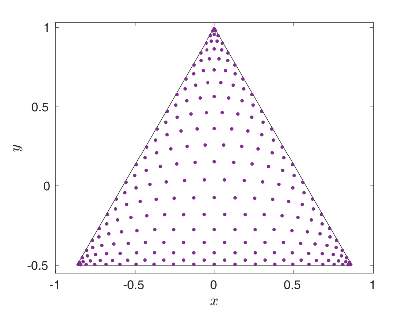
(a)

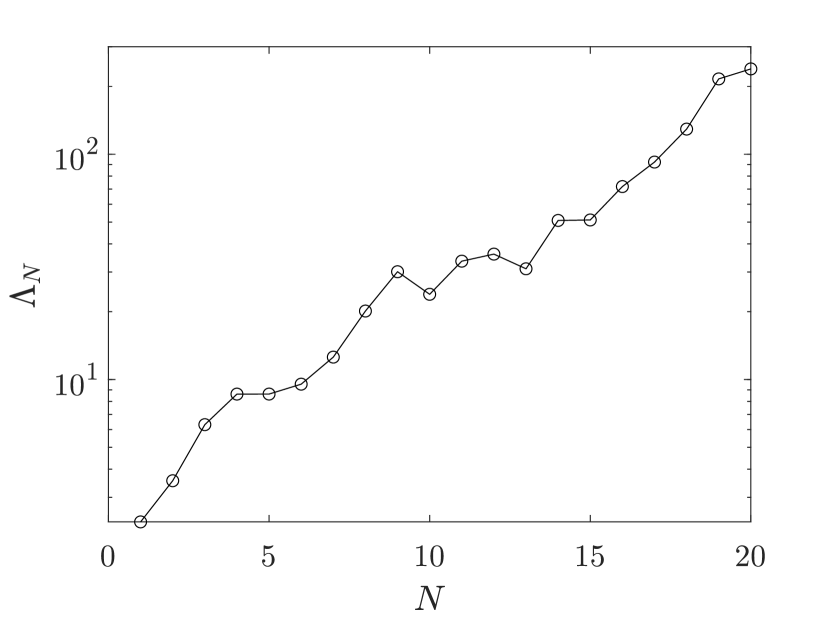
(b)

Figure 1: The 20th order Vioreanu-Rokhlin nodes over a triangle, and the associated Lebesgue constants for various orders of approximation.. The $x$-axis label $N$ denotes the order of approximation. One may observe in Figure 1(b) that the Lebesgue constant for the Vioreanu-Rokhlin nodes does not exhibit monotonic growth, which is due to the heuristic nature of the algorithm used to construct these nodes.

Now let $\widetilde{\Delta}\subset\mathbbm{R}^{2}$ be a star-shaped curved triangle with only one curved side, $\gamma:[0,L]\to\mathbbm{R}^{2}$ be the parameterization of the curved side of $\widetilde{\Delta}$, and $O\in\mathbbm{R}^{2}$ be the vertex opposite to the curved side. The blending function method [11] provides a smooth mapping from the standard simplex $\Delta^{0}=\{(x,y)\in\mathbbm{R}^{2}:0\leq x\leq 1,0\leq y\leq 1-x\}$ to the curved triangle $\widetilde{\Delta}$, defined by the formula

$$\rho(\xi,\eta):= \ (1-\xi-\eta)\cdot\gamma(L)+\xi\cdot\gamma(0)+\eta\cdot O$$

$$+ \frac{1-\xi-\eta}{1-\xi}\Bigl{(}\gamma\bigl{(}L(1-\xi)\bigr{)}-(1-\xi)\cdot\gamma(L)-\xi\cdot\gamma(0)\Bigr{)}.$$ (12)

To obtain a set of collocation points over $\widetilde{\Delta}$, we map the Vioreanu-Rokhlin nodes over $\Delta^{0}$ to $\widetilde{\Delta}$ via (12). We observe that the Lebesgue constant of resulting collocation points is also relatively small in magnitude when $\gamma$ is not too curved.

Similar to the 1-D case, the 2-D Vandermonde matrix (11) is also exponentially ill-conditioned. The following theorem provides a priori bounds for the monomial approximation error, which shows that the accuracy of approximation is essentially unrelated to the ill-conditioning of the matrix. Its proof is almost identical to the proof of Theorem 2.2 in [23].

Theorem 3.1.

Let $\Omega\subset\mathbbm{R}^{2}$ be a bounded domain, and let $F:\Omega\to\mathbbm{C}$ be an arbitrary function. Suppose that $P_{N}$ is the $N$th degree bivariate interpolating polynomial of $F$ for a given set of $\widetilde{N}$ distinct collocation points $Z:=\{(x_{j},y_{j})\}_{j=1,2,\dots,\widetilde{N}}\subset\Omega$. Let $V^{(N)}$, $a^{(N)}$ and $f^{(N)}$ be the same as introduced above. Suppose that there exists some constant $\gamma_{N}\geq 0$ such that the computed monomial coefficient vector $\widehat{a}^{(N)}:=(\widehat{a}_{00},\widehat{a}_{10},\widehat{a}_{01},\dots,\widehat{a}_{0N})^{T}\in\mathbbm{R}^{\widetilde{N}}$ satisfies

$$\bigl{(}V^{(N)}+\delta V^{(N)}\bigr{)}\widehat{a}^{(N)}=f^{(N)},$$ (13)

for some $\delta V^{(N)}\in\mathbbm{R}^{\widetilde{N}\times\widetilde{N}}$ with

$${\lVert\delta V^{(N)}\rVert}_{2}\leq u\cdot\gamma_{N},$$ (14)

where $u$ denotes machine epsilon. Let $\widehat{P}_{N}(x,y):=\sum_{j=0}^{N}\sum_{k=0}^{j}\allowbreak\widehat{a}_{j-k,k}\bigl{(}\frac{x-c}{s}\bigr{)}^{j-k}\bigl{(}\frac{y-d}{t}\bigr{)}^{k}$ be the computed monomial expansion. If the 2-norm of $(V^{(N)})^{-1}$ satisfies

$${\lVert(V^{(N)})^{-1}\rVert}_{2}\leq\frac{1}{2u\cdot\gamma_{N}},$$ (15)

then the 2-norm of the numerical solution $\widehat{a}^{(N)}$ is bounded by

$$\frac{2}{3}{\lVert a^{(N)}\rVert}_{2}\leq{\lVert\widehat{a}^{(N)}\rVert}_{2}\leq 2{\lVert a^{(N)}\rVert}_{2},$$ (16)

and the monomial approximation error can be quantified a priori by

$${\lVert F-\widehat{P}_{N}\rVert}_{L^{\infty}(\Omega)}\leq \,{\lVert F-P_{N}\rVert}_{L^{\infty}(\Omega)}+2u\cdot\gamma_{N}\Lambda_{N}{\lVert a^{(N)}\rVert}_{2},$$ (17)

where $\Lambda_{N}$ denotes the Lebesgue constant for $Z$.

When solving the Vandermonde system using a backward stable linear system solver, the set of assumptions (13) and (14) is satisfied with constant $\gamma_{N}=\mathcal{O}({\lVert V^{(N)}\rVert}_{2})$. Furthermore, based on the same analysis as in [23], one can show that $u\cdot{\lVert a^{(N)}\rVert}_{2}\lesssim{\lVert F-P_{N}\rVert}_{L^{\infty}(\Omega)}$ holds in most practical situations when ${\lVert(V^{(N)})^{-1}\rVert}_{2}$ satisfies the condition (15), from which it follows that the monomial basis is as good as an orthogonal polynomial basis for interpolation in such cases. Therefore, it is advisable to carefully select the monomial expansion center $(c,d)$ and the scaling factors $s$, $t$ to minimize the growth of both ${\lVert V^{(N)}\rVert}_{2}$ and ${\lVert(V^{(N)})^{-1}\rVert}_{2}$. Below, we provide an algorithm for choosing these constants.

Given an arbitrary bounded domain $\Omega$ in $\mathbb{R}^{2}$, we define $B$ to be the minimum bounding box of $\Omega$ (see Figure 2(a)). Then, we establish a local coordinate system centered at the midpoint of $B$, with the $x$- and $y$-axes aligned parallel to the sides of $B$. In this coordinate system, we set $c$ and $d$ to be zero, $s$ to be half the length of the longer side of $B$, and $t$ to be half the length of the shorter side of $B_{1}$. One can show that the entries of the resulting Vandermonde matrix $V^{(N)}$ are no larger than one in magnitude, which implies that the constant $\gamma_{N}$ is small. In addition, one can observe from Figure 2(b) that the condition (15) is satisfied for $N\lesssim 20$, regardless of the triangle’s aspect ratio.

In Section 5.1, we provide numerical experiments to demonstrate the feasibility of bivariate polynomial interpolation in the monomial basis.

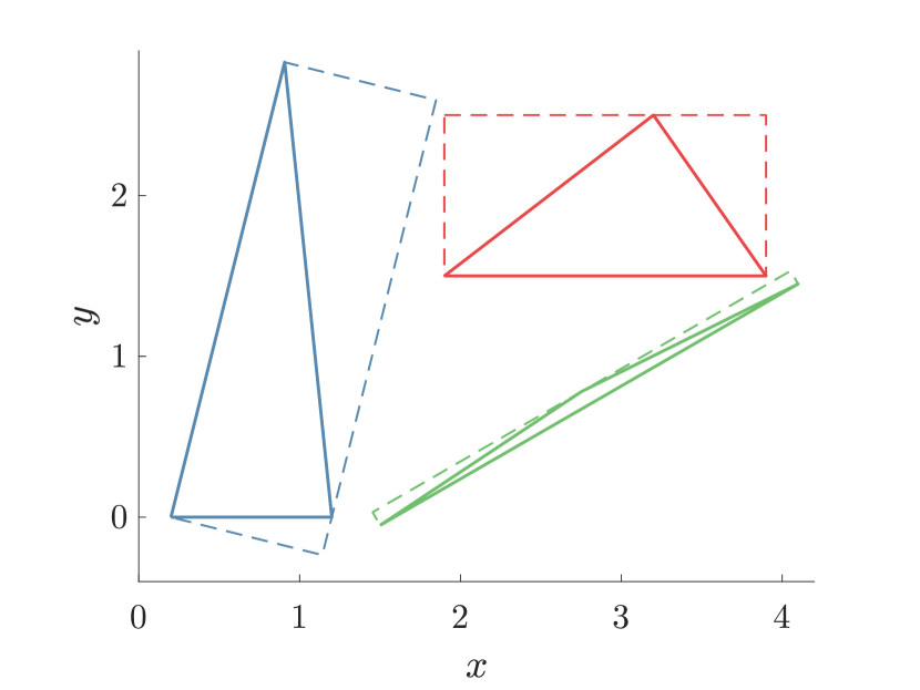
(a)

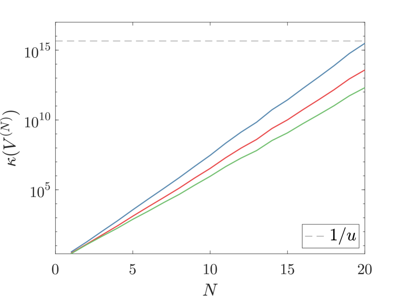
(b)

Figure 2: The growth of $\kappa(V^{(N)})$ for triangles with different aspect ratios. The colors of the triangles in Figure 2(a) correspond to the line colors depicted in Figure 2(b). The boxes in Figure 2(a) define the local coordinate for each triangle.

4 Numerical algorithm

In this section, we first present an algorithm for computing the Newtonian potential when the domain $\Omega$ is a (possibly curved) triangle. Then, we describe how to apply this algorithm to compute the Newtonian potential over a general domain. In the end, we show that our algorithm has linear time complexity.

4.1 Construction of the anti-Laplacian mapping

In this section, we present an algorithm for computing the anti-Laplacian of a bivariate monomial. With a slight abuse of notation, we denote the anti-Laplacian operator by $\nabla^{-2}$, which we define by the recurrence relations

$$\nabla^{-2}\Bigl{[}\Bigl{(}\frac{x-c}{s}\Bigr{)}^{m}\Bigr{]}= \,\frac{s^{2}}{(m+1)(m+2)}\Bigl{(}\frac{x-c}{s}\Bigr{)}^{m+2},$$ (18a)

$$\nabla^{-2}\Bigl{[}\Bigl{(}\frac{x-c}{s}\Bigr{)}^{m}\Bigl{(}\frac{y-d}{t}\Bigr{)}\Bigr{]}= \,\frac{s^{2}}{(m+1)(m+2)}\Bigl{(}\frac{x-c}{s}\Bigr{)}^{m+2}\Bigl{(}\frac{y-d}{t}\Bigr{)},$$ (18b)

for all $m\geq 0$, and

$$\nabla^{-2}\Bigl{[}\Bigl{(}\frac{y-d}{t}\Bigr{)}^{n}\Bigr{]}= \,\frac{t^{2}}{(n+1)(n+2)}\Bigl{(}\frac{y-d}{t}\Bigr{)}^{n+2},$$ (19a)

$$\nabla^{-2}\Bigl{[}\Bigl{(}\frac{x-c}{s}\Bigr{)}\Bigl{(}\frac{y-d}{t}\Bigr{)}^{n}\Bigr{]}= \,\frac{t^{2}}{(n+1)(n+2)}\Bigl{(}\frac{x-c}{s}\Bigr{)}\Bigl{(}\frac{y-d}{t}\Bigr{)}^{n+2},$$ (19b)

for all $n\geq 0$, and

$$\nabla^{-2}\Bigl{[}\Bigl{(}\frac{x-c}{s}\Bigr{)}^{m}\Bigl{(}\frac{y-d}{t}\Bigr{)}^{n}\Bigr{]}= \,\frac{s^{2}}{(m+2)(m+1)}\Bigl{(}\frac{x-c}{s}\Bigr{)}^{m+2}\Bigl{(}\frac{y-d}{t}\Bigr{)}^{n}$$

$$\,-\frac{s^{2}n(n-1)}{t^{2}(m+2)(m+1)}\nabla^{-2}\Bigl{[}\Bigl{(}\frac{x-c}{s}\Bigr{)}^{m+2}\Bigl{(}\frac{y-d}{t}\Bigr{)}^{n-2}\Bigr{]}$$ (20a)

$$= \,\frac{t^{2}}{(n+2)(n+1)}\Bigl{(}\frac{x-c}{s}\Bigr{)}^{m}\Bigl{(}\frac{y-d}{t}\Bigr{)}^{n+2}$$

$$\,-\frac{t^{2}m(m-1)}{s^{2}(n+2)(n+1)}\nabla^{-2}\Bigl{[}\Bigl{(}\frac{x-c}{s}\Bigr{)}^{m-2}\Bigl{(}\frac{y-d}{t}\Bigr{)}^{n+2}\Bigr{]},$$ (20b)

for all $m\geq 2,n\geq 2$. It is easy to verify that $\nabla^{2}\circ\nabla^{-2}=I$. Based on these recurrence relations, one can construct a mapping from the monomial coefficients of a bivariate polynomial of degree $N$ to the monomial coefficients of the anti-Laplacian of this polynomial. This mapping only has $\mathcal{O}(N^{2})$ non-zero entries, and should be stored in a sparse format.

Remark 4.1.

The identity (20a) produces a shorter sequence of recurrence relations when $m\geq n$, and vice versa for (20b).

4.2 Close and self-evaluation of Newtonian potential over a mesh element

Given a possibly curved triangle $\Delta_{1}$ and a function $f:\Delta_{1}\to\mathbbm{R}$, we first compute its bivariate interpolating polynomial in the monomial basis, as described in Section 3. By Green’s third identity (see Theorem 2.1), the Newtonian potential with density function $f$ over $\Delta_{1}$ at a given target $x\in\mathbbm{R}^{2}$ can be expressed as

$$\iint_{\Delta_{1}}G(x,y)f(y)\,\mathrm{d}A_{y}\approx \,\iint_{\Delta_{1}}G(x,y)P_{N}(y)\,\mathrm{d}A_{y}$$

$$= \,\varphi(x)\mathbbm{1}_{\Delta_{1}}(x)+\oint_{\partial\Delta_{1}}\Bigl{(}G(x,y)\frac{\partial\varphi}{\partial n_{y}}(y)-\frac{\partial G(x,y)}{\partial n_{y}}\varphi(y)\Bigr{)}\,\mathrm{d}\ell_{y},$$ (21)

where $P_{N}$ is the $N$th degree bivariate interpolating polynomial of $f$, and $\varphi:=\nabla^{-2}[P_{N}]$ is a bivariate polynomial of degree $(N+2)$ computed using the algorithm outlined in the previous section. Thus, it remains to compute the layer potentials $\int_{L_{i}}G(x,y)\frac{\partial\varphi}{\partial n_{y}}(y)\,\mathrm{d}\ell_{y}$ and $\int_{L_{i}}\frac{\partial G(x,y)}{\partial n_{y}}\varphi(y)\,\mathrm{d}\ell_{y}$ for $i=1$, $2$, $3$, where $L_{i}$ denotes the $i$th edge of $\Delta_{1}$. When $x$ is well-separated from $L_{i}$, these integrands are smooth, and (21) is computed using a standard quadrature rule. When $x$ is close to $L_{i}$, these integrands become nearly-singular, and the Helsing-Ojala method is used for the calculation (see Section 2.2). We note that the restriction of the anti-Laplacian $\varphi$ to a line segment is a univariate polynomial of degree $N+2$.

Remark 4.2.

It is well-known that Horner’s method evaluates a polynomial in the monomial basis with the fewest number of multiplications. However, Estrin’s scheme outperforms Horner’s method in terms of speed on a modern computer, as it effectively utilizes CPU pipelines.

4.3 Generalization to an arbitrary domain

Given a general planar region $\Omega$, we first discretize $\Omega$ into triangles and curved triangles using a standard off-the-shelf meshing algorithm. Then, we construct the anti-Laplacian of the density function in the form of a 2-D monomial expansion for each mesh element. We also compute the 1-D monomial expansion coefficients for the restriction of the anti-Laplacian and its normal derivatives to the edges of each element. At this stage, all of the required precomputations are completed.

Then, we use the point-based fast multipole method (FMM) [15] to compute the far field interactions. Typically, one uses 2-D quadrature rules over triangles to compute the far field interactions generated over mesh elements (see, for example, [22, 1]) and, thus, the number of quadrature nodes over each element for computing far field interactions is of order $\mathcal{O}(N^{2})$, where $N$ is the degree of the bivariate interpolating polynomial for the density function. We note, however, that in the far field, the layer potentials in Green’s third identity (5) can be computed efficiently and accurately by Gauss-Legendre rules. It follows that, in our algorithm, the number of quadrature nodes over each element is of order $\mathcal{O}(N)$. Finally, we compute the near and self-interactions using the algorithm presented in the previous section, and use the “subtract-and-add” method to remove the spurious contribution from the FMM (see [14] for details).

Remark 4.3.

Given two adjacent mesh elements, their far field quadrature nodes over their common edge coincide, and thus, one could merge the nodes in the FMM computation to reduce the number of sources by a factor of two. Similarly, one could merge the expansion coefficients of the two 1-D monomial expansions over the common edge of two elements to reduce the near interaction computational cost by a factor of two.

4.4 Time complexity analysis

In this section, we present the time complexity of our algorithm. Suppose that we construct a $p$th degree bivariate interpolating polynomial of the density function over each element. Consequently, each polynomial is represented by $(p+1)(p+2)/2=\mathcal{O}(p^{2})$ terms in the monomial basis. We estimate the various costs as follows.

Precomputation for each mesh element:

1. The computation of the 2-D monomial expansion coefficients of the density function takes $\mathcal{O}(p^{6})$ operations, since the cost is dominated by the factorization of a 2-D Vandermonde matrix of size $\mathcal{O}(p^{2})\times\mathcal{O}(p^{2})$.

2. The computation of the anti-Laplacian takes $\mathcal{O}(p^{3})$ operations.

3. The evaluation of the anti-Laplacian and its normal derivative at the $\mathcal{O}(p)$ collocation points on the edges of the mesh elements takes $\mathcal{O}(p^{3})$ operations.

4. The computation of the 1-D monomial expansions of the restriction of the anti-Laplacian and its normal derivatives takes $\mathcal{O}(p^{2})$ operations on a straight edge (as one can store and reuse the pivoted LU factorization of the 1-D Vandermonde matrix with Gauss-Legendre collocation nodes over $[-1,1]$), and takes $\mathcal{O}(p^{3})$ on a curved edge. We note that the total number of curved edges is generally far fewer than the total number of straight edges.

Close and self-evaluation of the Newtonian potential over a mesh element at a single target location:

1. It takes $\mathcal{O}(p)$ operations to evaluate the layer potentials on the right hand side of Green’s third identity (5), either by the Gauss-Legendre rule or the Helsing-Ojala method.

2. It takes $\mathcal{O}(p^{2})$ operations to evaluate the anti-Laplacian on the right hand side of Green’s third identity (5). This is only required by the self-evaluation.

Based on these estimates, we present the total number of operations required to evaluate the Newtonian potential over all of the discretization nodes over the domain $\Omega$. Suppose that $\Omega$ is discretized into $m$ mesh elements. Then, the number of discretization nodes $N_{\text{tot}}$ is of order $\mathcal{O}(p^{2}m)$. First, the precomputation takes $\mathcal{O}(p^{6}m)=\mathcal{O}(p^{4}N_{\text{tot}})$ operations. Second, the far field interaction costs (i.e., the FMM cost) are of order $\mathcal{O}(pm+N_{\text{tot}})$. Third, the near interaction computation takes $\mathcal{O}(pN_{\text{tot}})$ operations, as each discretization node is inside the near fields of a constant number of mesh elements. Finally, the self-interaction computation takes $\mathcal{O}(p^{2}N_{\text{tot}})$ operations. Since $p$ is generally a small constant, our algorithm has linear time complexity. Furthermore, we note that the constant associated with the precomputation is small (see Table 4), and the near and self-interaction computations are nearly instantaneous after the precomputations have been performed.

5 Numerical experiments

In this section, we illustrate the performance of the algorithm with several numerical examples. We implemented our algorithm in Fortran 77 and Fortran 90, and compiled it using the Intel Fortran Compiler, version 2021.6.0, with the -Ofast flag. We conducted all experiments on a ThinkPad laptop, with 16 GB of RAM and an Intel Core i7-10510U CPU.

We use the Vioreanu-Rokhlin rules [26], which are publicly available in [13]. We use the FMM library published in [12] in our implementation. We use the subroutines dgetrf and dgetrs (i.e., LU factorization with partial pivoting) from LAPACK as our linear system solver for the Vandermonde system. We make no use of parallelization. While we comment in Remark 4.3 that it is more efficient to loop through edges instead of triangles, these features are not implemented in our code, for the sake of simplicity.

We list the notation that appears in this section below.

• $S_{\text{exps}}$: The number of targets at which the Newtonian potential generated over a mesh element can be evaluated per second using our algorithm, after the precomputation.

• $S_{\text{adap}}$: The number of targets at which the Newtonian potential generated over a mesh element can be evaluated, per second, using adaptive integration.

• $E_{\text{exps}}$: The absolute error of the potential evaluation computed using our algorithm.

• $E_{\text{adap}}$: The absolute error of the potential evaluation computed using adaptive integration.

• $N_{\text{elem}}$: The number of mesh elements.

• $h_{0}^{\max}$: The maximum diameter of all mesh elements.

• $h_{0}^{\min}$: The minimum diameter of all mesh elements.

• $A^{\max}$: The maximum aspect ratio of all mesh elements. The aspect ratio of a triangle equals the ratio of its circumradius to twice its inradius.

• $N_{\text{ord}}$: The order of the bivariate polynomial approximation to the density function over each mesh element.

• $N_{\text{tot}}^{\text{tgt}}$: The total number of targets at which the Newtonian potential is evaluated.

• $N_{\text{tot}}^{\text{src}}$: The total number of sources (i.e., far field quadrature nodes).

• $T_{\text{geom}}$: The time spent on the geometric algorithms: quadtree constructions, nearby elements queries, etc. The mesh creation time is not counted.

• $T_{\text{init}}$: The time spent on the precomputations required by our algorithm.

• $T_{\mathcal{F}}$: The time spent on the far field interaction computation (i.e., the FMM computation).

• $T_{\mathcal{N}}$: The time spent on the near field interaction computation, including the subtraction of spurious contributions from the far field interaction computation (see [14, 22]).

• $T_{\mathcal{S}}$: The time spent on the self-interaction computation, including the subtraction of spurious contributions from the far field interaction computation (see [14, 22]).

• $T_{\text{tot}}$: The total time for the evaluation of the volume potential at all of the discretization nodes.

• $\frac{\#\text{tgt}}{\text{sec}}$: The number of targets at which the Newtonian potential can be evaluated per second using our algorithm, including the precomputation cost.

• $E_{\text{poi}}$: The largest absolute error of the solution to Poisson’s equation at all of the target nodes.

• $E_{\text{den}}$: The $L^{\infty}$ monomial approximation error of the density function over the whole domain, estimated by comparing the approximated function values at 40,000 uniformly sampled points over the domain with the true function values.

• $E_{\text{tol}}$: The error tolerance of the adaptive version of our algorithm. Used in the experiment with an inhomogeneous density function.

5.1 Bivariate polynomial interpolation in the monomial basis

In this section, we present numerical experiments to demonstrate the feasibility of bivariate polynomial interpolation in the monomial basis.

Let $\Delta_{1}$ be an equilateral triangle with vertices $(-1,0),(1,0)$ and $(0,\sqrt{3})$, and let $\Delta_{2}$ be a flattened triangle with vertices $(-1,0),(1,0)$ and $(0,\frac{1}{16})$. In Figures 3 and 4, we estimate $L^{\infty}$ errors of bivariate polynomial interpolation in the 2-D monomial basis and in the Koornwinder polynomial basis [3] (i.e., the orthogonal polynomial basis over a triangle) over the domains $\Delta_{1}$ and $\Delta_{2}$ with the Vioreanu-Rokhlin collocation points, for different orders of approximation $N$, by comparing the values of the two approximations with the true values of the function at 20,000 uniformly sampled points over the domain. We also report the extra numerical error that arises from the use of monomial basis (i.e., $u\cdot{\lVert a^{(N)}\rVert}_{2}$; see Theorem 3.1). One can observe that the use of the monomial basis induces essentially no extra loss of accuracy in both cases.

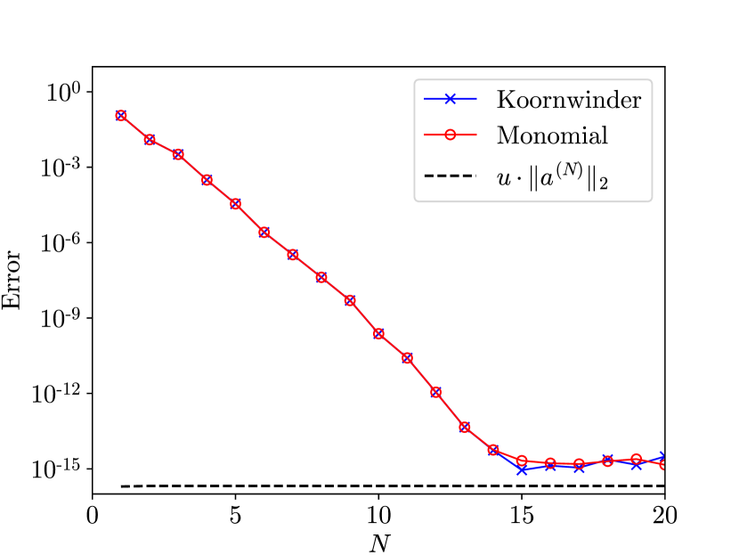
(a) $f(x,y)=e^{-(x^{2}+y^{2})/8}$

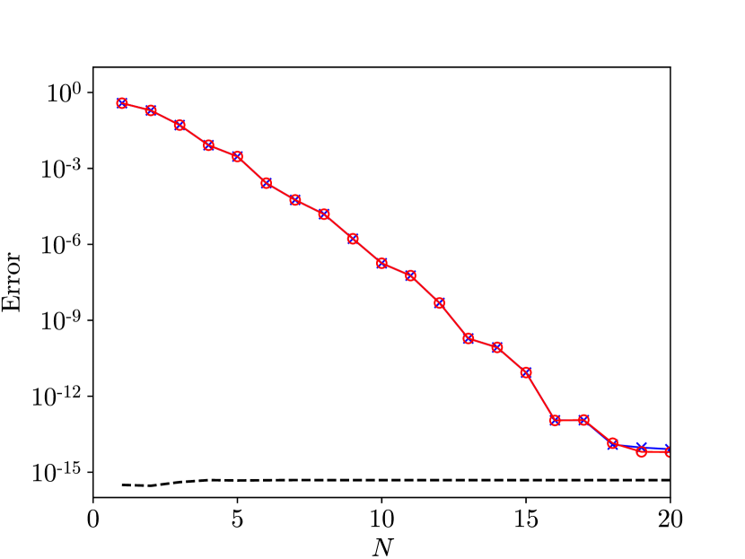
(b) $f(x,y)=\sin(\frac{1}{2}xy+x+y)$

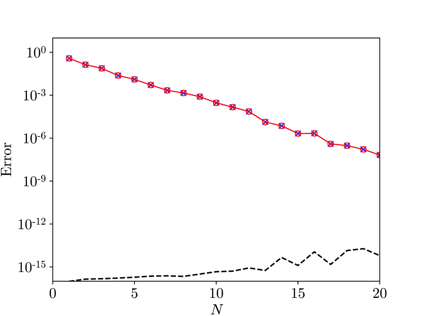
(c) $f(x,y)=\frac{1}{x^{2}+(y+1)^{2}}$

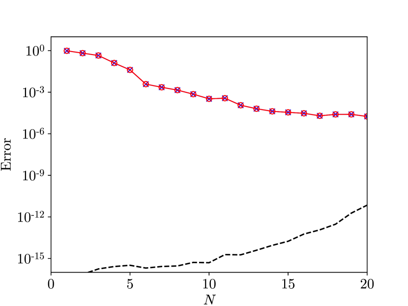
(d) $f(x,y)={\lvert x\rvert}^{5.5}$

Figure 3: Bivariate polynomial interpolation over the equilateral triangle $\Delta_{1}$ by monomials and Koornwinder polynomials.

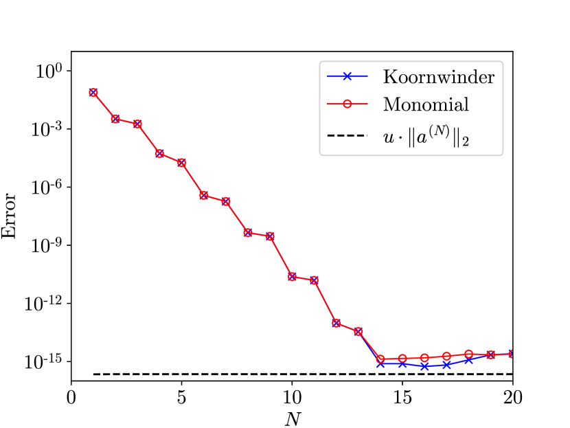
(a) $f(x,y)=e^{-(x^{2}+y^{2})/8}$

(b) $f(x,y)=\sin(\frac{1}{2}xy+x+y)$

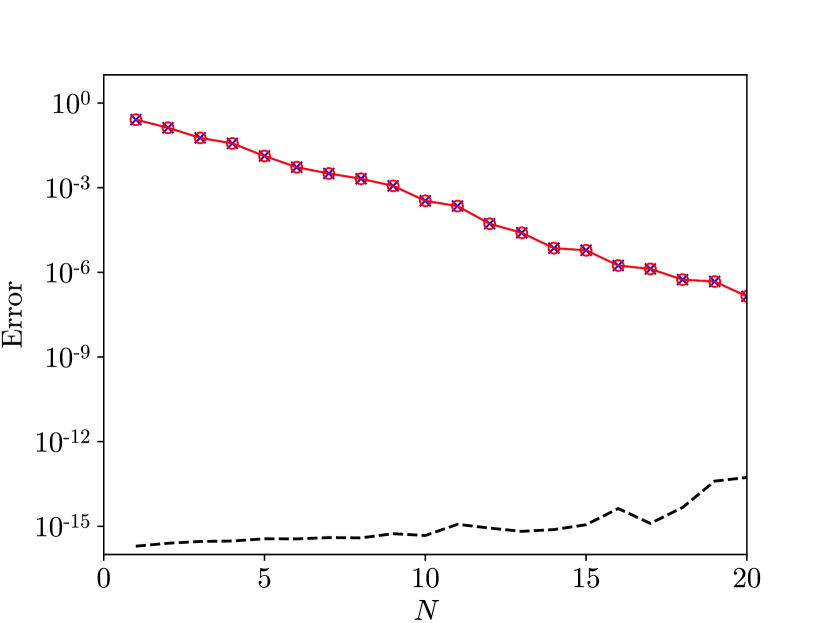
(c) $f(x,y)=\frac{1}{x^{2}+(y+1)^{2}}$

(d) $f(x,y)={\lvert x\rvert}^{5.5}$

Figure 4: Bivariate polynomial interpolation over the flattened triangle $\Delta_{2}$ by monomials and Koornwinder polynomials.

Now let $\widetilde{\Delta}$ be a curved triangle, given by the formula

$$\widetilde{\Delta}:=\{(r\cos\theta-1,r\sin\theta)\in\mathbbm{R}^{2}:0\leq r\leq 2,0\leq\theta\leq\pi/3\}.$$ (22)

We repeat the previous experiment on $\widetilde{\Delta}$, and show the results in Figure 5. One can observe that the performance of the monomial approximation over a curved triangle is almost identical to the triangle domain case.

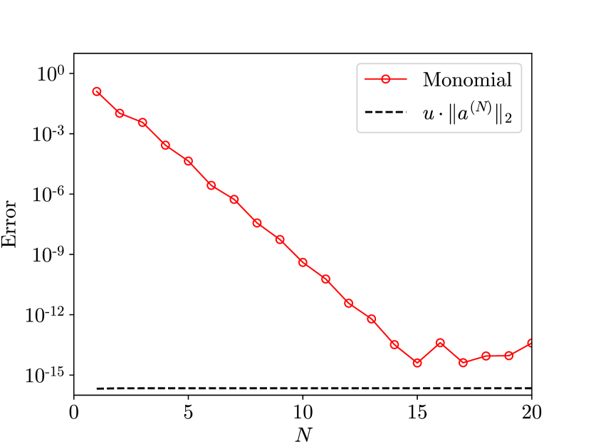
(a) $f(x,y)=e^{-(x^{2}+y^{2})/8}$

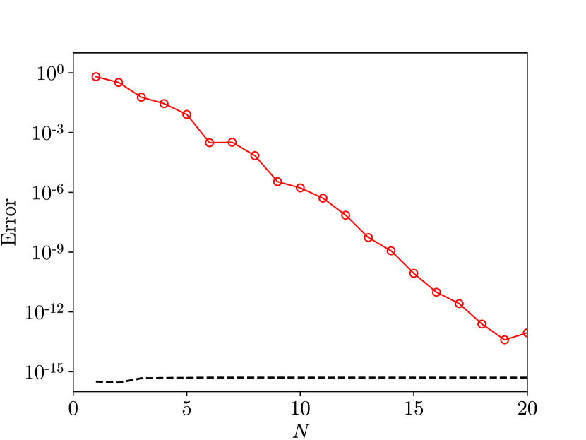
(b) $f(x,y)=\sin(\frac{1}{2}xy+x+y)$

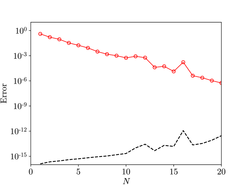
(c) $f(x,y)=\frac{1}{x^{2}+(y+1)^{2}}$

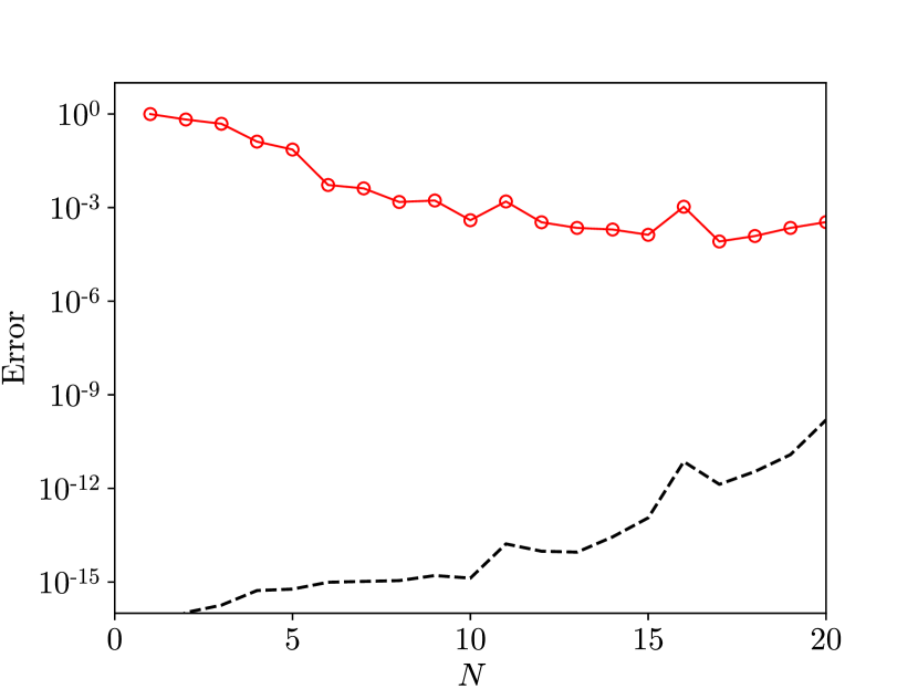
(d) $f(x,y)={\lvert x\rvert}^{5.5}$

Figure 5: Bivariate polynomial interpolation over the curved triangle element $\widetilde{\Delta}$ by monomials.

5.2 Newtonian potential generated over a mesh element

In this section, we compare our algorithm with adaptive integration for Newtonian potential evaluation. We set the domain to be $\Delta:=\{(x,y)\in\mathbbm{R}^{2}:0\leq x\leq 1,0\leq y\leq 1-x\}$, the density function to be $f(x,y)=\cos(5xy)+\sin(2x+1)+\cos(3y-1)$, and the target location to be $(0.5,-h)$, for various $h$. In the adaptive integration computation, we used the Vioreanu-Rokhlin rule of order $N_{\text{ord}}$, equipped with the error control technique introduced in [22] to align the error with the error of our algorithm. To make the adaptive integration speed independent of the complexity of the density function, we excluded the time spent on the density function evaluations on the first level, but included the time spent on interpolating the density function values to the next level (see [3] for a fast interpolation technique). Furthermore, we accelerated the application of the interpolation matrix by LAPACK, and fine-tuned the baseline to make the comparisons fair. The reference solutions were computed using extremely high-order adaptive integration. In Table 1, we report the speed-up of the close evaluation of the Newtonian potential obtained by our algorithm after the precomputation, compared to the conventional adaptive integration-based approach, for different orders of approximation. We do not include a similar experiment that demonstrates the speed-up of the self-evaluation, since a fair experiment requires the speed of the adaptive integration-based approach to be independent of the cost of evaluating the density function. We note that, even when the density function is a constant (so that its evaluation is free), the speed of the self-evaluation by our algorithm is significantly faster than the adaptive integration-based approach when the target point is close to the boundary of the domain. In Figure 6, we report the speeds for the close and self-evaluations, and of the precomputations, for various orders of approximations. In Figure 7, we show the plots of the computational errors of the Newtonian potential.

$N_{\text{ord}}$	$h$	$S_{\text{exps}}$	$S_{\text{adap}}$	$\frac{S_{\text{exps}}}{S_{\text{adap}}}$	$E_{\text{exps}}$	$E_{\text{adap}}$
8	$2\times 10^{-1}$	9.29$\times 10^{5}$	3.56$\times 10^{5}$	2.61	4.07$\times 10^{-8}$	1.37$\times 10^{-7}$
	$2\times 10^{-2}$	1.19$\times 10^{6}$	2.02$\times 10^{5}$	5.88	3.06$\times 10^{-8}$	9.73$\times 10^{-8}$
	$2\times 10^{-3}$	1.19$\times 10^{6}$	6.13$\times 10^{4}$	19.4	4.89$\times 10^{-8}$	2.78$\times 10^{-7}$
	$2\times 10^{-4}$	1.19$\times 10^{6}$	5.39$\times 10^{4}$	22.1	5.10$\times 10^{-8}$	5.35$\times 10^{-8}$
	$2\times 10^{-5}$	1.19$\times 10^{6}$	3.95$\times 10^{4}$	30.1	5.12$\times 10^{-8}$	7.03$\times 10^{-8}$
14	$2\times 10^{-1}$	1.04$\times 10^{6}$	5.07$\times 10^{4}$	20.6	9.42$\times 10^{-13}$	9.41$\times 10^{-13}$
	$2\times 10^{-2}$	1.04$\times 10^{6}$	1.51$\times 10^{4}$	69.0	1.69$\times 10^{-11}$	1.20$\times 10^{-11}$
	$2\times 10^{-3}$	1.04$\times 10^{6}$	8.21$\times 10^{3}$	127	2.27$\times 10^{-11}$	5.83$\times 10^{-11}$
	$2\times 10^{-4}$	1.04$\times 10^{6}$	5.64$\times 10^{3}$	185	2.34$\times 10^{-11}$	5.30$\times 10^{-11}$
	$2\times 10^{-5}$	1.04$\times 10^{6}$	4.09$\times 10^{3}$	255	2.35$\times 10^{-11}$	5.66$\times 10^{-11}$
20	$2\times 10^{-1}$	7.40$\times 10^{5}$	1.19$\times 10^{4}$	62.2	7.77$\times 10^{-16}$	1.00$\times 10^{-16}$
	$2\times 10^{-2}$	7.41$\times 10^{5}$	3.11$\times 10^{3}$	238	4.16$\times 10^{-16}$	8.33$\times 10^{-17}$
	$2\times 10^{-3}$	7.41$\times 10^{5}$	1.56$\times 10^{3}$	474	8.60$\times 10^{-16}$	2.03$\times 10^{-15}$
	$2\times 10^{-4}$	7.43$\times 10^{5}$	1.00$\times 10^{3}$	741	1.05$\times 10^{-15}$	6.38$\times 10^{-16}$
	$2\times 10^{-5}$	7.42$\times 10^{5}$	8.09$\times 10^{2}$	917	8.33$\times 10^{-16}$	5.83$\times 10^{-16}$

Table 1: The speed-up of close evaluation of Newtonian potentials generated over a single mesh element $\Delta$.

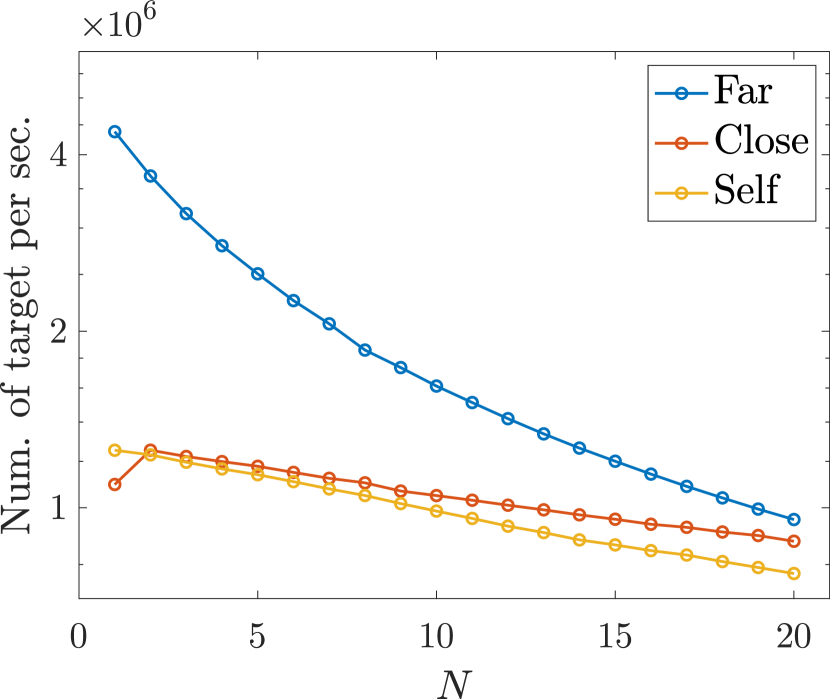
(a)

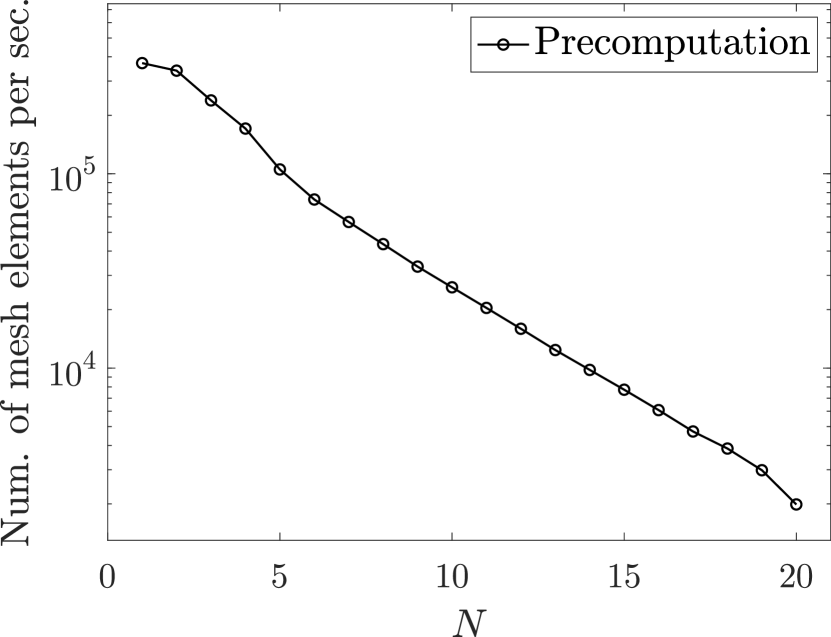
(b)

Figure 6: The speed of the far, close, and self-evaluations, and of the precomputations, over a single mesh element $\Delta$. The $x$-axis denotes the order of approximation. The $y$-axes in (a) and (b) denote the number of targets the volume potential can be evaluated at and the number of mesh elements that the precomputation can be executed on, per second, respectively. The label “Far” denotes the evaluation of the Newtonian potential via (5) by a Gauss-Legendre rule of order $N+2$ over every edge of the mesh element. The labels “Close” and “Self” denote the close and self-evaluation of the Newtonian potential via (5) by the Helsing-Ojala method of order $N+2$ over every edge of the mesh element.

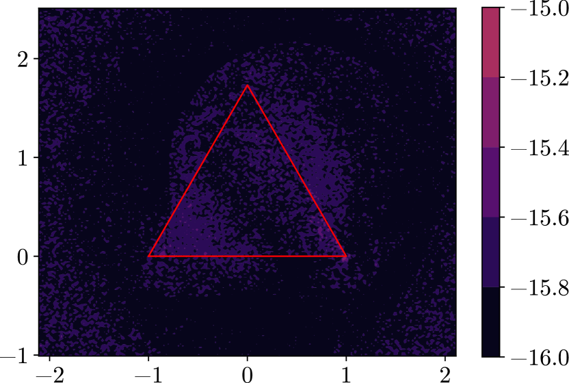
(a)

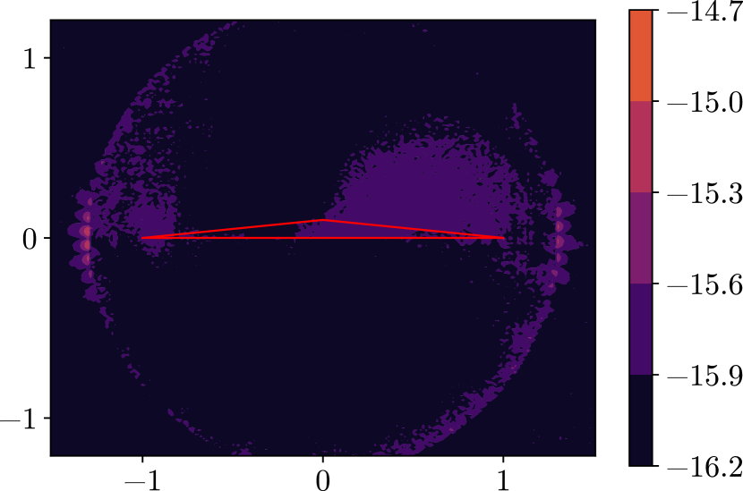
(b)

Figure 7: Error contours. We set the density function to be $f(x,y)=\sin(\frac{1}{2}xy+x+y)$, and the orders of the 2-D and 1-D monomial approximations to be 20 and 22, respectively.

5.3 Poisson’s equation

In this section, we report the performance of our Newtonian potential evaluation algorithm in the context of solving Poisson’s equation

$$\nabla^{2}\varphi= \,f\text{ in }\Omega,$$

$$\varphi= \,g\text{ on }\partial\Omega,$$ (23)

where

$$f(x,y)=9\cos(9x)\sin(6y)+16\cos\bigl{(}16y+\frac{8}{5}\bigr{)}-12\sin(12x),$$ (24)

and

$$g(x,y)=\varphi(x,y)|_{\partial\Omega}= \,\Bigl{(}\frac{1}{12}\sin(12x)-\frac{1}{16}\cos\bigl{(}16y+\frac{8}{5}\bigr{)}-\frac{1}{13}\cos(9x)\sin(6y)\Bigr{)}\Big{|}_{\partial\Omega},$$ (25)

for the domain $\Omega$ is displayed in Figure 8. The boundary of this domain was created by the following procedure. First, we fit a $C^{\infty}$ curve through a collection of points using the algorithm described in [28], and then up-sampled the curve to produce a new collection of data points. The final curve was constructed by interpolating these new points using the interpolation formula and $C^{\infty}$ interpolatory basis introduced in [27], where the basis functions are translates of the product of the sinc function and the Gaussian $\exp(-ax^{2})$, with the parameter $a=0.1$. The final curve can be recreated from this interpolation formula, together with the data points, which we provide in https://doi.org/10.5281/zenodo.8401488. Once the boundary of $\Omega$ has been constructed, a mesh is created on $\Omega$ using the Gmsh mesh generator. To ensure that the boundary is well-resolved by the triangle mesh, we post-process the resulting mesh by performing additional subdivision of curved triangles on high curvature regions.

It is easy to verify that the solution $\varphi$ to Poisson’s equation (23) can be expressed as the sum of the Newtonian potential $u$ with density function $f$ over the domain $\Omega$, and the solution to the Laplace equation

$$\nabla^{2}u^{h}= \,0\quad\text{in $\Omega$},$$

$$u^{h}= \,g-u\quad\text{on $\partial\Omega$}.$$ (26)

In our implementation, we first compute $u$ using our algorithm, and then solve the Laplace equation (26) using the boundary integral equation method [25].

In our first experiment, we aim to validate both the convergence rate and the computational efficiency of our algorithm. To achieve this, we discretize the domain $\Omega$ using a quasi-uniform triangular mesh. We provide the problem sizes in Tables 2 and 3. Subsequently, we present a detailed performance analysis of our algorithm in Table 4, and visualize its convergence rate in Figure 9. Our results demonstrate that our algorithm exhibits the anticipated order of convergence. Additionally, when the order is not extremely high (e.g., $\leq 14$), the time spent on precomputation is small, and the computational costs associated with near and self-interaction are comparable to those of the far field interaction computation.

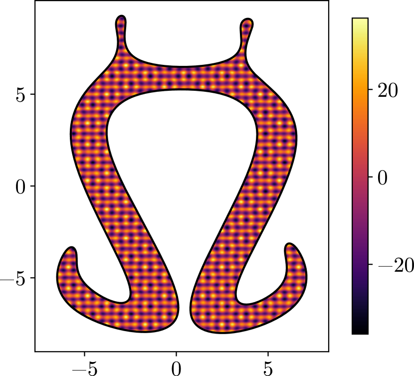
(a)

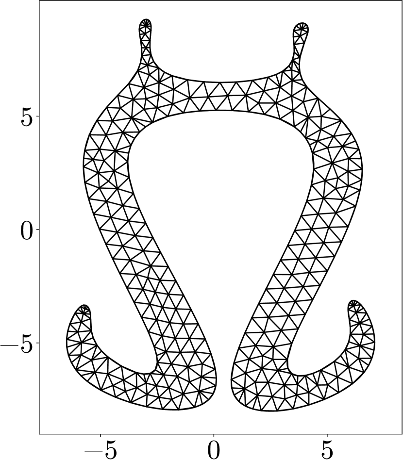
(b)

Figure 8: The domain $\Omega$, the density function $f$, and an example mesh where $h_{0}^{\max}=0.99$.

$h_{0}^{\max}$	$N_{\text{elem}}$	$A^{\max}$	$h_{0}^{\min}/h_{0}^{\max}$
0.99	542	1.96	0.16
0.55	1844	4.20	0.17
0.28	6964	45.5	0.17

Table 2: The total number of mesh elements, the maximum diameter (i.e., $h_{0}^{\max}$), aspect ratio (i.e., $A^{\max}$) of mesh elements, and the ratio between the largest and smallest triangles (i.e., $h_{0}^{\min}/h_{0}^{\max}$), for different meshes used in Poisson’s equation experiment. Note that the ratio between the minimum diameter and the maximum diameter of mesh elements is small, because the mesh size has to be smaller inside the two lobes (see Figure 8).

$N_{\text{ord}}$	$h_{0}^{\max}$	$N_{\text{tot}}^{\text{src}}$	$N_{\text{tot}}^{\text{tgt}}$	$\frac{N_{\text{tot}}^{\text{src}}}{N_{\text{tot}}^{\text{tgt}}}$
8	0.99	17886	24390	73.3%
	0.55	60852	82980
	0.28	229812	313380
14	0.99	27642	65040	42.5%
	0.55	94044	221280
	0.28	355164	835680
20	0.99	37398	125202	29.9%
	0.55	127236	425964
	0.28	480516	1608684

Table 3: The total number of sources and targets for different orders of approximation $N_{\text{ord}}$ and for different mesh sizes $h_{0}$ used in Poisson’s equation experiment. We note that the total number of the mesh elements equals $552$, $1844$, $6898$ when $h_{0}=0.6$, $0.3$, $0.15$, respectively. The sources are the Gauss-Legendre nodes of order $N_{\text{ord}}+2$ along the boundaries of the mesh elements, and the targets are the Vioreanu-Rokhlin nodes of order $N_{\text{ord}}$ over all mesh elements. The values in the last column are equal to $6(N_{\text{ord}}+3)/\bigl{(}(N_{\text{ord}}+1)\cdot(N_{\text{ord}}+2)\bigr{)}$, and show the reduction in the number of far field quadrature nodes, when the far field interactions are computed using Green’s third identity.

$N_{\text{ord}}$	$h_{0}^{\max}$	$T_{\text{geom}}$	$T_{\text{init}}$	$T_{\mathcal{F}}$	$T_{\mathcal{N}}$	$T_{\mathcal{S}}$	$T_{\text{tot}}$	$\frac{\#\text{tgt}}{\text{sec}}$	$E_{\text{poi}}$
8	$0.99$	0.02	0.03	0.17	0.04	0.02	0.29	8.53$\times 10^{4}$	1.49$\times 10^{-3}$
	$0.55$	0.06	0.07	0.60	0.15	0.08	0.97	8.57$\times 10^{4}$	1.01$\times 10^{-6}$
	$0.28$	$0.24$	0.26	1.72	0.67	0.32	3.21	9.77$\times 10^{4}$	1.90$\times 10^{-9}$
14	$0.99$	0.05	0.09	0.34	0.15	0.08	0.71	9.13$\times 10^{4}$	4.98$\times 10^{-7}$
	$0.55$	0.18	0.31	1.05	0.81	0.36	2.70	8.19$\times 10^{4}$	9.05$\times 10^{-12}$
	$0.28$	0.58	0.93	3.65	2.70	1.15	9.01	9.27$\times 10^{4}$	3.75$\times 10^{-12}$
20	$0.99$	0.20	0.96	0.99	0.33	0.18	2.67	4.69$\times 10^{4}$	7.71$\times 10^{-11}$
	$0.55$	0.31	2.84	2.34	1.09	0.62	7.21	5.91$\times 10^{4}$	7.39$\times 10^{-12}$
	$0.28$	1.26	10.5	7.20	4.46	2.55	26.0	6.19$\times 10^{4}$	5.18$\times 10^{-12}$

Table 4: Performance of our algorithm for solving Poisson’s equation. The smallest value of $E_{\text{poi}}$ we report is $3.75\times 10^{-12}$. We found that the loss of several digits accuracy was due to the condition number associated with the calculation of the curvature of $\partial\Omega$, which is represented as a global $C^{\infty}$ curve. Note that the meshes for different values of $N_{\text{ord}}$ with the same value of $h_{0}^{\max}$ are identical.

(a) 8th order

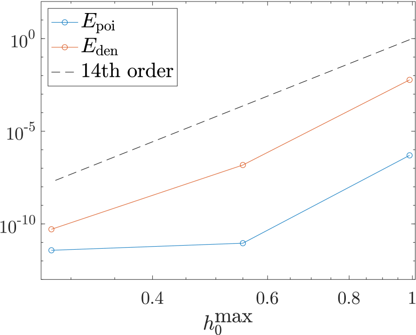
(b) 14th order

Figure 9: Order of convergence. We refer the readers to the caption of Table 4 for the reason why the error does not decay to machine precision in Figure (b).

In the following example, we assess the performance and accuracy of our algorithm for an inhomogeneous density function and a domain featuring multiscale features. Specifically, we define the density function as the combination of a smooth function and three highly localized spikes, given by:

$$f(x,y)= \,2-32\sin(4(x+y))+$$

$$\,2\sum_{i=1}^{3}e^{-c_{i}^{2}(x-a_{i})^{2}-d_{i}^{2}(y-b_{i})^{2}}\bigl{(}-c_{i}^{2}-d_{i}^{2}+2c_{i}^{4}(x-a_{i})^{2}+2d_{i}^{4}(y-b_{i})^{2}\bigr{)},$$ (27)

where $(a_{1},b_{1},c_{1},d_{1}):=(-3,6,10,10)$, $(a_{2},b_{2},c_{2},d_{2}):=(2,-7,5,10)$ and $(a_{3},b_{3},c_{3},d_{3}):=(3.8,8.6,15,20)$. We set the boundary condition of Poisson’s equation to be

$$g(x,y)=\varphi(x,y)|_{\partial\Omega}= \,\sin(4(x+y))+(x^{2}-3y+8)+\sum_{i=1}^{3}e^{-c_{i}^{2}(x-a_{i})^{2}-d_{i}^{2}(y-b_{i})^{2}}\Big{|}_{\partial\Omega}.$$ (28)

Additionally, we introduce a tiny lobe to the previously defined domain $\Omega$. The density function and the domain are visualized in Figure 10. We also set the order $N_{\text{ord}}$ of our algorithm to be 14.

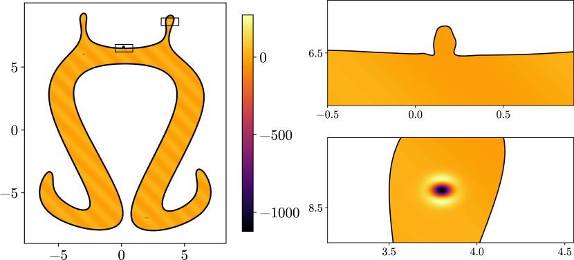
Figure 10: The domain $\Omega$ with a tiny lobe, and the inhomogeneous density function $f$.

To accurately represent the inhomogeneous density function, we refine the initial mesh by 1-to-4 subdivisions until the density function over each element can be approximated by a polynomial of degree 14 within a specified error tolerance. To resolve the tiny lobe, we use Gmsh to subdivide the lobe and its neighborhood until we achieve the desired reduction in error. We provide the problem sizes and the performance of our algorithm in Table 5, and plot the corresponding meshes in Figure 11. Note that the error tolerance required for resolving the density is typically several orders of magnitude larger than $E_{\text{tol}}$.

Remark 5.1.

In our experiments, we found that the time spent on the far field interaction computation performed by the FMM has a high variance, so we ran the program several times and reported the experiment with the smallest FMM computation time. We note that the runtimes of all other parts of our algorithm have low variance.

(a) Error tolerance $=10^{-5}$

(b) Error tolerance $=10^{-10}$

Figure 11: The meshes used in the Poisson’s equation experiments for a multiscale domain and an inhomogeneous density function.

$E_{\text{tol}}$	$N_{\text{elem}}$	$A^{\max}$	$T_{\text{geom}}$	$T_{\text{init}}$	$T_{\mathcal{F}}$	$T_{\mathcal{N}}$	$T_{\mathcal{S}}$	$T_{\text{tot}}$	$\frac{\#\text{tgt}}{\text{sec}}$	$E_{\text{poi}}$
$10^{-5}$	1076	5.05	0.15	0.19	0.60	0.19	0.15	1.27	1.02$\times 10^{5}$	5.75$\times 10^{-5}$
$10^{-10}$	3258	2.41	1.59	0.51	1.88	1.93	0.72	6.63	6.09$\times 10^{4}$	8.57$\times 10^{-10}$

Table 5: Performance of our algorithm for solving Poisson’s equation when the domain has a multiscale feature and when the density function is inhomogeneous. In this experiment, $N_{\text{ord}}=14$. We note that the time spent on the geometric algorithms (i.e., $T_{\text{geom}}$) is substantially higher than the one in the previous examples. This is because our geometric algorithm is not optimized for multiscale meshes. The near field interaction computation takes much longer for the same reason.

6 Conclusions and further directions

In this paper, we present a simple and efficient high-order algorithm for the rapid evaluation of Newtonian potentials over a general planar domain. Furthermore, we provide a justification for employing a monomial basis in the context of high-order (up to order 20) bivariate polynomial interpolation. This choice serves as a crucial component of our algorithm, despite being commonly regarded as infeasible.

We note that our algorithm can be generalized to compute the Helmholtz (or Yukawa) volume potential, provided that the anti-Helmholtizian (or anti-Yukawaian) of a bivariate polynomial can be approximated accurately, and that the Helmholtz (or Yukawa) layer potentials over the boundaries of mesh elements can be efficiently computed to high accuracy (see, for example, [18, 9]). Furthermore, the use of polynomial interpolation in the monomial basis and Green’s third identity generalize in a straightforward way to 3-D domains, but efficient algorithms for the evaluation of surface Newtonian potentials are an area of active research.

7 Acknowledgements

We are deeply grateful to Travis Askham, Shidong Jiang, Manas Rachh, and the anonymous referees for their valuable advice and insightful discussions.

References

- [1] T. G. Anderson, H. Zhu, and S. Veerapaneni, A Fast, High-Order Scheme for Evaluating Volume Potentials on Complex 2D Geometries via Area-to-Line Integral Conversion and Domain Mappings, J. Comput. Phys., 472 (2023), pp. 111688.
- [2] T. Askham, and A. J. Cerfon, An Adaptive Fast Multipole Accelerated Poisson Solver for Complex Geometries, J. Comput. Phys., 344 (2017), pp. 1–22.
- [3] J. Bremer, and Z. Gimbutas, A Nyström Method for Weakly Singular Integral Operators on Surfaces, J. Comput. Phys., 231.14 (2012), pp. 4885–4903.
- [4] J. Bremer, Z. Gimbutas, and V. Rokhlin, A Nonlinear Optimization Procedure for Generalized Gaussian Quadratures, SIAM J. Sci. Comput., 32.4 (2010), pp. 1761–1788.
- [5] O. P. Bruno, and J. Paul, Two-Dimensional Fourier Continuation and Applications, SIAM J. Sci. Comput. 44.2 (2022), pp. A964–992.
- [6] F. Ethridge, Fast Algorithms for Volume Integrals in Potential Theory, Ph.D. dissertation, New York University.
- [7] F. Ethridge, and L. Greengard, A New Fast-Multipole Accelerated Poisson Solver in Two Dimensions, SIAM J. Sci. Comput., 23.3 (2001), pp. 741–760.
- [8] C. Epstein, and S. Jiang. A Stable, Efficient Scheme for Function Extensions on Smooth Domains in , arXiv:2206.11318, 2022.
- [9] F. Fryklund, L. af Klinteberg, and A. K. Tornberg, An Adaptive Kernel-Split Quadrature Method for Parameter-Dependent Layer Potentials, Adv. Comput. Math., 48.2 (2022), pp. 1–17.
- [10] F. Fryklund, E. Lehto, and A. K. Tornberg, Partition of Unity Extension of Functions on Complex Domains, J. Comput. Phys. 375 (2018), pp. 57–79.
- [11] W. J. Gordon, and C. A. Hall, Construction of Curvilinear Co-Ordinate Systems and Applications to Mesh Generation, Int. J. Numer. Methods Eng., 7.4 (1973), pp. 461–477.
- [12] Z. Gimbutas, and L. Greengard, Computational Software: Simple FMM Libraries for Electrostatics, Slow Viscous Flow, and Frequency-Domain Wave Propagation, Commun. Comput. Phys., 18.2 (2015), pp. 516–528.
- [13] Z. Gimbutas, and H. Xiao, Quadratures for triangles, squares, cubes and tetrahedra, https://github.com/zgimbutas/triasymq (2020).
- [14] L. Greengard, M. O’Neil, M. Rachh, and F. Vico, Fast Multipole Methods for the Evaluation of Layer Potentials with Locally-Corrected Quadratures, J. Comput. Phys.: X, 10 (2021), pp. 100092.
- [15] L. Greengard, and V. Rokhlin, A Fast Algorithm for Particle Simulations, J. Comput. Phys., 135.2 (1997), pp. 280–292.
- [16] L. af Klinteberg, and A. H. Barnett. Accurate Quadrature of Nearly Singular Line Integrals in Two and Three Dimensions by Singularity Swapping, BIT Numer. Math. 61.1 (2021): 83–118.
- [17] J. Helsing, and R. Ojala. On the Evaluation of Layer Potentials Close to Their Sources, J. Comput. Phys. 227.5 (2008): 2899–2921.
- [18] J. Helsing, and A. Holst. Variants of an Explicit Kernel-Split Panel-Based Nyström Discretization Scheme for Helmholtz Boundary Value Problems, Adv. Comput. Mathe. 41.3 (2015), pp. 691–708.
- [19] A. Mayo, The Rapid Evaluation of Volume Integrals of Potential Theory on General Regions, J. Comput. Phys., 100.2 (1992), pp. 236–245.
- [20] S. Nintcheu Fata, Treatment of Domain Integrals in Boundary Element Methods, Appl. Numer. Math., 62.6 (2012), pp. 720–735.
- [21] P. W. Patridge, C. A. Brebbia, L. W. Wrobel, The Dual Reciprocity Boundary Element Method, Computational Mechanics Publication, Southampton, 1992.
- [22] Z. Shen, and K. Serkh, Accelerating Potential Evaluation over Unstructured Meshes in Two Dimensions, arXiv:2205.04401 (2022).
- [23] Z. Shen, and K. Serkh, Is polynomial interpolation in the monomial basis unstable?, arXiv:2212.10519 (2022).
- [24] J. D. Towers, A Source Term Method for Poisson Problems on Irregular Domains, J. Comput. Phys. 361 (2018), pp. 424–441.
- [25] P. G. Martinsson, Fast Direct Solvers for Elliptic PDEs, CBMS-NSF Conference Series, vol. CB96. SIAM, Philadelphia, 2019.
- [26] B. Vioreanu, and V. Rokhlin, Spectra of Multiplication Operators as a Numerical Tool, SIAM J. Sci. Comput., 36.1 (2014), pp. A267–288.
- [27] R. J. Zhang, and W. Ma, An efficient scheme for curve and surface construction based on a set of interpolatory basis functions, ACM T. Graph., 30.2 (2011), pp. 1–11.
- [28] M. Zhao, and K. Serkh, A Continuation Method for Fitting a Bandlimited Curve to Points in the Plane, arXiv:2301.04241 (2023).
- [29] H. Zhu, Fast, High-Order Accurate Integral Equation Methods and Application to PDE-Constrained Optimization, PhD thesis, University of Michigan (2021).