Spacetimes with no position drift

Abstract

This paper compares three criteria for a spacetime to be free of position drift: those by Hasse and Perlick (HP), Krasiński and Bolejko (KB) and Korzyński and Kopiński (KK). A spacetime having no position drift means that every observer sees all light sources in unchanging directions. The following is shown: (1) The HP criterion is a necessary condition for the KK criterion to apply. (2) If the spacetime metric obeys the Einstein equations with a perfect fluid source, then another necessary condition for the KK criterion is the Weyl tensor being zero. (3) Result (2) points to the Stephani metric, so it is shown that this metric obeys an equation which is still one more necessary condition for the KK criterion. (4) The general Szekeres metrics become drift-free by the KK criterion only in the Friedmann limit. (5) The HP and KB criteria coincide, and the HP zero-drift condition imposes on the Stephani metric the same restriction as found by Krasiński and Bolejko (KB). The relations between the three criteria are displayed and compared in a diagram.

1 Motivation and summary

Some time ago, this author noted that in an inhomogeneous Universe a generic observer should see distant light sources drift across the sky, unlike in Robertson – Walker metrics. The drift is caused by the shearing and rotating motion of the cosmic matter that sweeps the light rays passing through it, so the direction from which a ray reaches an observer changes (relative to other light sources) with the observer’s time. The no-drift condition was that light rays coming at different times to an observer ${\cal O}$ from the emitter ${\cal E}$ intersect on their way always the same intermediate world lines of cosmic matter. Equations governing the drift were derived for the class I Szekeres models [1] – [3] in Ref. [4] and for the Barnes [5] and the expanding Stephani models [6] in Refs. [7] and [8]. The angular rate of the drift calculated in an exemplary Lemaître [9] – Tolman [10] (L–T) model ($\approx 10^{-6}$ arc seconds per year [4]) was on the verge of detectability for the then-being-constructed Gaia satellite. A no-drift condition defined in a way equivalent to that of Ref. [4] was discussed earlier by Hasse and Perlick [11] without reference to explicit solutions of Einstein’s equations.

Recently, Korzyński and collaborators published a series of papers in which they discussed a (seemingly) differently defined drift in a general spacetime [12] – [14]. They derived a formula for the position drift, not just a zero-drift condition. Their formula is the Fermi – Walker derivative along the observer world line of the unit direction vector to the light source. The aim of the present paper is to relate to each other the sets of results by the Korzyński – Kopiński (KK) [12], Hasse – Perlick (HP) [11] and Krasiński – Bolejko (KB) [4, 7] teams.

In Sec. 2, the semi-null tetrad defined at a point by an observer velocity $u^{\alpha}$ and a past-directed null vector $p^{\alpha}$ [12] is described. Formulae are given for the tetrad ${e_{i}}^{\alpha}$, the inverse tetrad ${e^{i}}_{\alpha}$, the scalar metric $\eta_{ij}$, the inverse scalar metric $\eta^{ij}$, and for the tetrad components of $u^{\alpha}$ and $p^{\alpha}$.

In Sec. 3, the position drift formulae are quoted from [12] and explained.

In Sec. 4 it is noted that zero drift by the HP definition is a necessary condition for zero drift by the KK definition. Then, in the same section and Appendix A it is shown that if the cosmic matter is a perfect fluid and the metric obeys the Einstein equations with this fluid as a source, then zero drift in the KK sense implies zero Weyl tensor.

All conformally flat perfect fluid metrics are known, they are the Stephani metrics [6, 15]. It is shown in Sec. 5 and Appendix B that they obey Eqs. (5) and (4), which are other necessary conditions for the KK zero drift.

In Sec. 6 it is shown that the Szekeres metrics are drift-free in the KK sense only in the Friedmann limit. This agrees with the result of Ref. [4].

In Sec. 7 it is shown that the KB definition of zero drift [4, 7] coincides with HP’s [11]. It is also verified that the HP definition applied to the expanding Stephani metric leads to the same (axially symmetric) subcase as the KB definition.

In Sec. 8 the relations between the HP, KB and KK approaches and their applications to the Stephani metric are explained and discussed in more detail, and displayed in a diagram.

Section 9 contains a brief summary of all the results.

The signature $(+---)$ will be used throughout most of the paper, except where comparisons with Ref. [12] are made.

2 The semi-null tetrad

The spacetimes considered here contain world lines of light emitters ${\cal E}$ and observers ${\cal O}$ with four-velocities $u_{\cal E}^{\alpha}$ and $u_{\cal O}^{\alpha}$, and light rays with tangent vectors $p^{\alpha}$. Occasionally, we refer to a third observer with four-velocity $U^{\alpha}$.

At each point where an observer world line and a light ray intersect, a semi-null tetrad (SNT) [13] of vectors can be introduced, on which tensors can be projected. Tetrad indices will be denoted by small latin letters $i,j,\dots=0,1,2,3$, tensor indices by Greek letters. Numerical values of tetrad indices will have a hat above them. The tetrad indices running through the two values $\widehat{1}$ and $\widehat{2}$ will be denoted by $A,B,C,\dots$.

The contravariant vectors of the SNT are chosen as follows:

$${e_{\widehat{0}}}^{\alpha} = u^{\alpha},$$ (1)

$${e_{A}}^{\alpha}, A=1,2,$$ (2)

$${e_{\widehat{3}}}^{\alpha} = p^{\alpha},$$ (3)

where $u^{\alpha}$ is a timelike unit vector ($u^{\alpha}u_{\alpha}=1$), $p^{\alpha}$ is a null vector ($p^{\alpha}p_{\alpha}=0$), and ${e_{A}}^{\alpha}$ are two spacelike unit vectors, orthogonal to each other and to both $u^{\alpha}$ and $p^{\alpha}$, so $g_{\alpha\beta}{e_{A}}^{\alpha}{e_{B}}^{\beta}=-\delta_{AB}$, ${e_{A}}^{\alpha}p_{\alpha}={e_{A}}^{\alpha}u_{\alpha}=0$, not otherwise specified. The ${e_{A}}^{\alpha}$ are defined at ${\cal O}$ and parallely transported along $p^{\alpha}$.

The tetrad metric $\eta_{ij}=g_{\alpha\beta}{e_{i}}^{\alpha}{e_{j}}^{\beta}$ is then

$$\eta_{\widehat{0}\widehat{0}}=1,\quad\eta_{\widehat{0}\widehat{1}}=\eta_{\widehat{0}\widehat{2}}=0,\quad\eta_{\widehat{0}\widehat{3}}=u_{\rho}p^{\rho},$$ (4)

$$\eta_{\widehat{1}\widehat{1}}=\eta_{\widehat{2}\widehat{2}}=-1,$$ (5)

$$\eta_{\widehat{1}\widehat{2}}=\eta_{\widehat{1}\widehat{3}}=\eta_{\widehat{2}\widehat{3}}=\eta_{\widehat{3}\widehat{3}}=0.$$ (6)

The inverse metric to $\eta_{ij}$ is

$$\eta^{\widehat{0}\widehat{0}}=\eta^{\widehat{0}\widehat{1}}=\eta^{\widehat{0}\widehat{2}}=0,\quad\eta^{\widehat{0}\widehat{3}}=1/u_{\rho}p^{\rho},$$ (7)

$$\eta^{\widehat{1}\widehat{1}}=\eta^{\widehat{2}\widehat{2}}=-1,$$ (8)

$$\eta^{\widehat{1}\widehat{2}}=\eta^{\widehat{1}\widehat{3}}=\eta^{\widehat{2}\widehat{3}}=0,$$ (9)

$$\eta^{\widehat{3}\widehat{3}}=-1/\left(u_{\rho}p^{\rho}\right)^{2}.$$ (10)

Thus, the covariant tetrad ${e^{i}}_{\alpha}=\eta^{is}g_{\alpha\rho}{e^{s}}_{\rho}$ is

$${e^{\widehat{0}}}_{\alpha} = p_{\alpha}/\left(u_{\rho}p^{\rho}\right),$$ (11)

$${e^{\widehat{1}}}_{\alpha} = -e_{{\widehat{1}}\alpha},\quad{e^{\widehat{2}}}_{\alpha}=-e_{{\widehat{2}}\alpha},$$ (12)

$${e^{\widehat{3}}}_{\alpha} = u_{\alpha}/\left(u_{\rho}p^{\rho}\right)-p_{\alpha}/\left(u_{\rho}p^{\rho}\right)^{2}.$$ (13)

The tetrad components of $u^{\alpha}$ and $p^{\alpha}$ are

$$u_{\widehat{0}} = 1,\quad u_{\widehat{3}}=u_{\rho}p^{\rho},\quad u_{\widehat{1}}=u_{\widehat{2}}=0,$$ (14)

$$u^{\widehat{0}} = 1,\quad u^{\widehat{1}}=u^{\widehat{2}}=u^{\widehat{3}}=0,$$ (15)

$$p_{\widehat{0}} = u_{\rho}p^{\rho},\quad p_{\widehat{1}}=p_{\widehat{2}}=p_{\widehat{3}}=0,$$ (16)

$$p^{\widehat{0}} = p^{\widehat{1}}=p^{\widehat{2}}=0,\quad p^{\widehat{3}}=1.$$ (17)

3 Position drift according to Ref. [12]

We recall the definitions of the basic notions introduced in Ref. [12].

At a point ${\it P}$ of a manifold a future-directed timelike vector $u^{\alpha}$ (which is the four-velocity of an observer) and a past-directed null vector $p^{\alpha}$ (which is tangent to a light ray reaching the observer) define the unit spacelike vector $r^{\alpha}$ pointing from ${\it P}$ to the light source:

$$r^{\alpha}=u^{\alpha}-p^{\alpha}/\left(p^{\rho}u_{\rho}\right).$$ (1)

The Fermi – Walker (FW) transport of a vector $V^{\alpha}$ along a unit timelike vector field $U^{\alpha}$ ($U^{\alpha}U_{\alpha}=1$) is such, by which the component of $V^{\alpha}$ lying in the $\{U^{\alpha},\dot{U}^{\alpha}\}$ plane, where $\dot{U}^{\alpha}\ {\overset{\rm def}{=}}\ U^{\rho}{U^{\alpha}};_{\rho}$, remains in this plane (so $V^{\alpha}$ does not rotate around $U^{\alpha}$). Then $V^{\alpha}$ obeys [16]

$$U^{\rho}V^{\alpha};_{\rho}=\left(V^{\rho}U_{\rho}\right)\dot{U}^{\alpha}-\left(V^{\rho}\dot{U}_{\rho}\right)U^{\alpha}\ {\overset{\rm def}{=}}\ {\overset{*}{V}}{}^{\alpha}.$$ (2)

If $U^{\alpha}$ is geodesic, then $\dot{U}^{\alpha}={\overset{*}{V}}{}^{\alpha}=0$ and the FW and parallel transports coincide. The Fermi-Walker derivative $\delta_{U}$ is defined by

$$(\delta_{U}V)^{\alpha}\ {\overset{\rm def}{=}}\ U^{\rho}V^{\alpha};_{\rho}-{\overset{*}{V}}{}^{\alpha},$$ (3)

so that $(\delta_{U}V)^{\alpha}=0$ when $V^{\alpha}$ is FW-transported along $U^{\alpha}$. Note that $(\delta_{U}U)^{\alpha}=0$.

The FW transport and FW derivative can be generalised to arbitrary tensor fields [12] and then it follows that $\delta_{U}g_{\alpha\beta}=0$ for any metric $g_{\alpha\beta}$ and any vector field $U^{\alpha}$. From this it follows that $\delta_{U}\left(g_{\alpha\beta}P^{\alpha}Q^{\beta}\right)=0$ for any FW-transported vector fields $P^{\alpha}$ and $Q^{\beta}$, so the FW transport preserves the angle between $P^{\alpha}$ and $Q^{\beta}$.

The FW derivative along the observer’s world line will be denoted $\delta_{\cal O}$.

Let a geodesic $G$ belong to a one-parameter family $F_{G}$ of geodesics, and let $p^{\alpha}$ be the vector field tangent to $G$. Then the field of vectors $\xi^{\alpha}$ pointing from points on $G$ toward neighbouring geodesics in $F_{G}$ is called geodesic deviation vector field and obeys the geodesic deviation equation

$${\cal G}\left[\xi\right]^{\mu}\ {\overset{\rm def}{=}}\ \nabla_{p}\left(\nabla_{p}\xi^{\mu}\right)-{R^{\mu}}_{\alpha\beta\nu}p^{\alpha}p^{\beta}\xi^{\nu}=0,$$ (4)

where $\nabla_{p}\xi^{\mu}\ {\overset{\rm def}{=}}\ p^{\rho}{\xi^{\mu}};_{\rho}$ and ${R^{\mu}}_{\alpha\beta\nu}$ is the curvature tensor. The definition of $\xi^{\mu}$ implies

$$\left(\nabla_{\xi}p\right)^{\mu}=\left(\nabla_{p}\xi\right)^{\mu},$$ (5)

which means that the fields $p^{\alpha}$ and $\xi^{\alpha}$ are surface-forming.

The definition of geodesic deviation applies to any bundle of geodesics, but in the following the geodesics will be null.

Imagine a bundle of past-directed rays emanating from the same observation event and let $\lambda$ be the affine parameter on them. Take one ray as the reference and consider the deviation vectors $\xi^{\alpha}$ along it. What matters in calculating the position drift of an observed source are the projections $\xi^{A}={{e^{A}}}_{\mu}\xi^{\mu}$ of $\xi^{\mu}$ on the 2-dimensional planes orthogonal to $p^{\mu}$ and to $u_{\cal O}^{\mu}$. Since the rays converge to the same point, we have $\xi^{A}(\lambda_{\cal O})=0$ at the observer, and then $\xi^{A}(\lambda)$ at any other $\lambda$ is uniquely defined by ${e^{A}}_{\mu}\left(\nabla_{\xi}p\right)^{\mu}={e^{A}}_{\mu}\left(\nabla_{p}\xi\right)^{\mu}={{\rm d}{\xi^{A}}}/{{\rm d}{\lambda}}$ (we assume there are no caustics between the observer and the light source). Since (4) is linear in $\xi^{\mu}$, the Jacobi matrix ${{\cal D}^{A}}_{B}$ exists such that

$$\xi^{A}(\lambda)={{\cal D}^{A}}_{B}(\lambda)\nabla_{p}\xi^{B}(\lambda_{\cal O}).$$ (6)

The ${{\cal D}^{A}}_{B}$ maps vectors tangent to the past light cone at ${\cal O}$ to vectors attached at other points along the rays. Since the mapping is 1 – 1, the inverse mapping also exists.

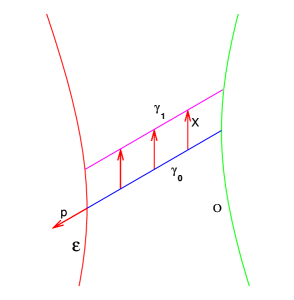
Figure 1: The emitter ${\cal E}$ keeps sending light rays to the observer ${\cal O}$; two such rays, $\gamma_{0}$ and $\gamma_{1}$, are shown. $X$ is the geodesic deviation vector field along $\gamma_{0}$ and $p$ is the past-directed tangent vector field to $\gamma_{0}$. (This is simplified Fig. 8 from Ref. [12]. )

Now let a source ${\cal E}$ send rays $\gamma_{0},\gamma_{1},\dots$ that intersect the observer world line ${\cal O}$, as in Fig. 1. The corresponding geodesic deviation field $X^{\mu}$, called observation time vector [12], is collinear with the observer velocity $u_{\cal O}^{\alpha}$ at ${\cal O}$ and with the emitter velocity $u_{\cal E}^{\alpha}$ at ${\cal E}$. We choose the affine parameters on the rays so that $\lambda=\lambda_{\cal O}$ at all points of intersection with the observer world line, and $\lambda=\lambda_{\cal E}$ at all points of intersection with the emitter world line. Then $X^{\mu}$ obeys ${\cal G}[X]^{\mu}=0$ and the initial conditions [12]

$$X^{\mu}(\lambda_{\cal O})=u^{\mu}_{\cal O},\qquad X^{\mu}(\lambda_{\cal E})=\frac{u^{\mu}_{\cal E}}{1+z},$$ (7)

where $z$ is the redshift along $\gamma_{0}$ between ${\cal E}$ and ${\cal O}$. We split $X^{\mu}$ as follows

$$X^{\mu}=\widehat{u}^{\mu}_{\cal O}+m^{\mu}+\phi^{\mu},$$ (8)

where $\widehat{u}^{\mu}_{\cal O}$ is the observer four-velocity parallely transported along $p^{\mu}$ from ${\cal O}$ to the running point on $\gamma$, while $m^{\mu}$ and $\phi^{\mu}$ obey

$${\cal G}[m]^{\mu} = {R^{\mu}}_{\alpha\beta\nu}p^{\alpha}p^{\beta}\widehat{u}^{\nu}_{\cal O},$$ (9)

$${\cal G}[\phi]^{\mu} = 0,$$ (10)

with the initial conditions

$$m^{\mu}(\lambda_{\cal O}) = 0,$$ (11)

$$\nabla_{p}m^{\mu}(\lambda_{\cal O}) = 0,$$ (12)

$$\phi^{\mu}(\lambda_{\cal O}) = 0,$$ (13)

$$\phi^{\mu}(\lambda_{\cal E}) = \frac{u^{\mu}_{\cal E}}{1+z}-\left.\widehat{u}^{\mu}_{\cal O}\right|_{\cal E}-m^{\mu}_{\cal E}.$$ (14)

Now $\phi^{\mu}(\lambda)$ can be calculated along $\gamma$ using (6) [12]. Knowing all this, the position drift of the light source is calculated to be [12]

$$\delta_{\cal O}r^{A} = \frac{1}{p_{\sigma}u_{\cal O}^{\sigma}}\ {\cal D}^{-1}{(\lambda_{\cal E})^{A}}_{B}\left(\frac{u^{B}}{1+z}-\widehat{u}_{\cal O}^{B}-m^{B}\right)_{\cal E}+w_{\cal O}^{A},$$ (15)

$$\equiv \frac{1}{p_{\sigma}u_{\cal O}^{\sigma}}\ {\cal D}^{-1}{(\lambda_{\cal E})^{A}}_{B}\phi^{B}\left(\lambda_{\cal E}\right)+w_{\cal O}^{A}$$

where $w_{\cal O}^{\mu}$ is the observer’s acceleration. The vector field $U^{\alpha}$ defining the tetrad for (15) need not coincide with $u_{\cal E}^{\alpha}$, but if it does then $u_{\cal E}^{B}=0$.

Since $\phi^{\mu}$ obeys (10) and (13), we can apply (6) to it, then

$$\delta_{\cal O}r^{A}=\frac{1}{p_{\sigma}u_{\cal O}^{\sigma}}\ \left(\nabla_{p}\phi^{A}\right)_{\cal O}+w_{\cal O}^{A}.$$ (16)

4 Implications of $\delta_{\cal O}r^{A}=0$ in (3.16)

The FW derivative preserves the scalar products of vectors, so $0=\delta_{\cal O}\left(r_{\mu}r^{\mu}\right)=2r_{\mu}\delta_{\cal O}r^{\mu}$, i.e., $\delta_{\cal O}r^{\mu}$ is orthogonal to $r^{\mu}$. It is also orthogonal to $u_{\cal O}^{\mu}$ because $\delta_{\cal O}u_{\cal O}^{\mu}=0$ (see the remark under (3)). Consequently, when $\delta_{\cal O}r^{A}=0$, the whole 4-dimensional $\delta_{\cal O}r^{\mu}=0$. Then, from the paragraph under (3) it follows that angles between the directions to any pair of light sources will remain constant in observer’s time – which is the HP [11] criterion for zero position drift. This means that the spacetimes that are drift-free in the KK sense are necessarily drift-free also in the HP sense. We will discuss the latter in Sec. 7. We first investigate a consequence of $\delta_{\cal O}r^{A}=0$ in (16).

In a zero-drift spacetime $X^{\mu}$ must be everywhere tangent to a surface formed by the world-lines of the cosmic medium. Consequently, $X^{A}=0$ and the change of $X^{\mu}$ along $p^{\mu}$ must also be tangent to this surface; i.e.,

$${\nabla_{p}X}^{\mu}=p^{\rho}{X^{\mu}};_{\rho}=fX^{\mu}+gp^{\mu},$$ (1)

where $f$ and $g$ are functions on the spacetime. The field $X^{\mu}$ obeys (4):

$$\left(\nabla_{p}\nabla_{p}X\right)^{\mu}-{R^{\mu}}_{\alpha\beta\nu}p^{\alpha}p^{\beta}X^{\nu}=0.$$ (2)

From (1) we have ${\nabla_{p}\nabla_{p}X}^{\mu}=\left({\nabla_{p}f}+f^{2}\right)X^{\mu}+\left(fg+{\nabla_{p}g}\right)p^{\mu}$, so

$$\left({\nabla_{p}f}+f^{2}\right)X^{\mu}+\left(fg+{\nabla_{p}g}\right)p^{\mu}={R^{\mu}}_{\alpha\beta\nu}p^{\alpha}p^{\beta}X^{\nu}.$$ (3)

Projecting this on $p^{\mu}$ we obtain ${\nabla_{p}f}+f^{2}=0$. Finally then

$$\left(fg+{\nabla_{p}g}\right)p^{\mu}={R^{\mu}}_{\alpha\beta\nu}p^{\alpha}p^{\beta}X^{\nu}.$$ (4)

We project (4) on the ${e^{A}}_{\mu}$ vectors that obey ${e^{A}}_{\mu}p^{\mu}=0$. The result is

$${R^{A}}_{\alpha\beta\nu}p^{\alpha}p^{\beta}X^{\nu}=0.$$ (5)

But (5) is not equivalent to (2) – it is only a subset of consequences of (2). Consequently, conclusions drawn from (5) will not fully represent (2), they will only be necessary conditions for (2). We will come back to this in Sec. 5.

We replace the coordinate summation indices with the tetrad summation indices and recall that $p^{\alpha}={e_{\widehat{3}}}^{\alpha}$. Then (5) becomes

$${R^{A}}_{\widehat{3}\widehat{3}i}\ X^{i}=0.$$ (6)

The component $X^{\widehat{3}}$ gives zero contribution to (6) (and is zero anyway), $X^{A}=0$, so what remains of (6) is ${R^{A}}_{\widehat{3}\widehat{3}\widehat{0}}X^{\widehat{0}}=0$. But from (15) $X^{\widehat{0}}=u^{\widehat{0}}/(1+z)\neq 0$. Thus, (6) implies ${R^{A}}_{\widehat{3}\widehat{3}\widehat{0}}=0$, and so, using (4) – (6):

$${R^{A\widehat{0}}}_{\widehat{3}\widehat{0}}\equiv{R^{A}}_{\widehat{3}\widehat{3}\widehat{0}}\ /u_{\rho}p^{\rho}=0.$$ (7)

For the Weyl tensor ${C^{\alpha\beta}}_{\gamma\delta}$ we have in tetrad components [3]

$${R^{ij}}_{kl}={C^{ij}}_{kl}-\frac{1}{2}\delta^{ijr}_{kls}\left({{R}^{s}}_{r}-\frac{1}{4}\ {\delta^{s}}_{r}R\right)+\frac{1}{12}\ \delta^{ij}_{kl}R,$$ (8)

where ${R^{i}}_{j}$ is the Ricci tensor and $R={R^{s}}_{s}$. Using (8) in (7) we find:

$${R^{A\widehat{0}}}_{\widehat{3}\widehat{0}}={C^{A\widehat{0}}}_{\widehat{3}\widehat{0}}+\frac{1}{2}\ {R^{A}}_{\widehat{3}}=0.$$ (9)

This simplifies when the cosmic matter is a perfect fluid (this assumption underlies all cosmological models) and the Einstein equations are obeyed

$${R^{i}}_{j}=\kappa\left[(\epsilon+p)u^{i}u_{j}-\frac{1}{2}(\epsilon-p){\delta^{i}}_{j}\right],$$ (10)

where $\kappa=8\pi G/c^{4}$, $\epsilon$ is the energy density and $p$ is the pressure. In the frame (1) – (3) $u^{A}=0$ and ${\delta^{A}}_{\widehat{3}}=0$, so ${R^{A}}_{\widehat{3}}=0$, and

$${C^{A}}_{\widehat{3}\widehat{3}\widehat{0}}={C^{A}}_{\alpha\beta\gamma}\ p^{\alpha}p^{\beta}u^{\gamma}=0.$$ (11)

This must hold for an arbitrary null vector $p^{\alpha}$, but only for that one $u^{\alpha}$ which is tangent to the cosmic matter flow line. It is shown in Appendix A that the requirement of (11) holding for all null fields $p^{\alpha}$ leads to the whole Weyl tensor being zero. Thus the conclusion is

Conclusion 1

For spacetimes in which the cosmic fluid is perfect and obeys the Einstein equations (10) the direction drift as defined by (16) is zero for all comoving observers only if the spacetime is conformally flat. $\square$

The conformally flat perfect fluid metrics are all explicitly known, they are the Stephani metrics [15, 6]. In general, the perfect fluid in them moves with acceleration, but in the limit of zero acceleration the expanding Stephani metric reduces to the general Robertson – Walker (RW) metric, while the expansion-free one trivializes to the Einstein universe which is a subcase of RW; see Sec. 5 here. Hence:

Conclusion 2

The only perfect fluid spacetimes in which the fluid moves geodesically and in which the direction drift as defined by (16) is zero for all comoving observers are the Robertson – Walker ones:

$${\rm d}s^{2}={\rm d}t^{2}-R^{2}(t)\left[\frac{{\rm d}r^{2}}{1-kr^{2}}+r^{2}\left({\rm d}\vartheta^{2}+\sin^{2}\vartheta{\rm d}\varphi^{2}\right)\right].$$ (12)

5 The Stephani [6, 15] metrics obey (3.16) with $\delta_{\cal O}r^{A}=0$

From (16), $\delta_{\cal O}r^{A}=0$ implies

$$w_{\cal O}^{A}=-\frac{1}{p_{\sigma}u_{\cal O}^{\sigma}}\ \left(\nabla_{p}\phi^{A}\right)_{\cal O}.$$ (1)

From (8) we have $\phi^{A}=X^{A}-\widehat{u}_{\cal O}^{A}-m^{A}$. But $\widehat{u}_{\cal O}^{\alpha}$ is parallely transported along $p^{\alpha}$, so $\left(\nabla_{p}\widehat{u}_{\cal O}\right)^{A}=0$, and from (12) $\left(\nabla_{p}m\right)^{A}\left(\lambda_{\cal O}\right)=0$. Consequently,

$$\left(\nabla_{p}\phi\right)_{\cal O}^{A}=\left(\nabla_{p}X\right)_{\cal O}^{A}.$$ (2)

In a drift-free spacetime $X^{\alpha}=u^{\alpha}/(1+z)$ on each ray. Thus

$$\left(\nabla_{p}X\right)_{\cal O}^{A}=\left.\frac{\left(\nabla_{p}u\right)^{A}}{1+z}\right|_{\cal O}-\frac{u^{A}_{\cal O}}{(1+z)^{2}}\ \nabla_{p}z.$$ (3)

But $u^{A}_{\cal O}=\left({e^{A}}_{\mu}u^{\mu}\right)_{\cal O}=0$ and $z=0$ at the observer. Therefore

$$\left(\nabla_{p}X\right)_{\cal O}^{A} = \left(\nabla_{p}u\right)^{A}_{\cal O},$$ (4)

$$w_{\cal O}^{A} = -\frac{1}{p_{\sigma}u_{\cal O}^{\sigma}}\ \left(\nabla_{p}u\right)^{A}_{\cal O}.$$ (5)

Note that $u^{A}_{\cal O}=0$ does not imply $(\nabla_{p}u)^{A}_{\cal O}=0$.

We will show here that the Stephani metrics obey (1), so zero Weyl tensor and a perfect fluid source constitute together a sufficient condition for (1) to hold. For a while we switch to the signature $(-+++)$ that was used in Ref. [12]. The expanding Stephani metric is

$${\rm d}s^{2}=-\left(\frac{FV,_{t}}{V}\right)^{2}{\rm d}t^{2}+\frac{1}{V^{2}}\ \left({\rm d}x^{2}+{\rm d}y^{2}{\rm d}z^{2}\right),$$ (6)

where

$$V=\frac{1}{R(t)}\ \left\{1+\frac{1}{4}\ k(t)\left[\left(x-x_{0}(t)\right)^{2}+\left(y-y_{0}(t)\right)^{2}+\left(z-z_{0}(t)\right)^{2}\right]\right\},$$ (7)

the functions $R(t)$, $k(t)$, $x_{0}(t)$, $y_{0}(t)$ and $z_{0}(t)$ being all arbitrary. It obeys the Einstein equations with a perfect fluid source, the mass density $\rho$ and pressure $p$ are

$$\kappa c^{2}\rho=3C^{2}(t),\qquad\kappa p=-3C^{2}(t)+2CC,_{t}V/V,_{t},\qquad\kappa\ {\overset{\rm def}{=}}\ 8\pi G/c^{4},$$ (8)

where the arbitrary function $C(t)$ is related to the other ones by

$$C^{2}=kR^{2}+1/F^{2}.$$ (9)

The velocity $u^{\alpha}$ and acceleration $w^{\alpha}={u^{\alpha}};_{\rho}u^{\rho}$ fields in (6) are

$$u^{\alpha}=\frac{V}{FV,_{t}}\ {\delta^{\alpha}}_{0},$$ (10)

$$w^{0}=0,\qquad w^{I}=\frac{V}{V,_{t}}\ \left(VV,_{tI}-V,_{t}V,_{I}\right),$$ (11)

where $I=1,2,3,(x^{1},x^{2},x^{3})=(x,y,z)$. (The spatial coordinate index $I$ is not to be confused with the tetrad index $A$.)

The $A$ components in (5) are projections of $w_{\cal O}^{\alpha}$ and $\left(\nabla_{p}u\right)^{\alpha}$ on the vectors ${e_{A}}^{\alpha}$ of the tetrad discussed in Sec. 2. Let $q^{\alpha}$ be any of the ${e_{A}}^{\alpha}$. Since it is orthogonal at ${\cal O}$ to the $u^{\alpha}$ of (10), it must have $q^{0}=0$. Then, orthogonality to $p^{\alpha}$ in the metric (6) means

$$p^{1}q^{1}+p^{2}q^{2}+p^{3}q^{3}=0.$$ (12)

The projection of $\left(\nabla_{p}u\right)^{\alpha}$ on $q^{\alpha}$ (i.e., one of the $(\nabla_{p}u)^{A}$) at ${\cal O}$ is

$$(\nabla_{p}u)^{q}_{\cal O}=g_{\alpha\beta}q_{\cal O}^{\alpha}(\nabla_{p}u)^{\beta}_{\cal O}=\nabla_{p}\left(g_{\alpha\beta}q^{\alpha}u^{\beta}\right)_{\cal O}=\frac{1}{V^{2}}\ \sum_{I=1}^{3}q^{I}_{\cal O}\left(\nabla_{p}u\right)^{I}_{\cal O}.$$ (13)

We have

$$\left(\nabla_{p}u\right)^{I}_{\cal O}=\left(p^{\rho}{u^{I}};_{\rho}\right)_{\cal O}=\left(p^{\rho}{u^{I}},_{\rho}\right)_{\cal O}+\left(p^{\rho}\mbox{\small$\begin{Bmatrix}I\ \\ 0\rho\ \end{Bmatrix}$}u^{0}\right)_{\cal O},$$ (14)

$$u^{I}=0\qquad{\rm everywhere\ in\ the\ coordinates\ of\ (\ref{5.6})},$$ (15)

$$\mbox{\small$\begin{Bmatrix}I\\ \ 00\end{Bmatrix}$}={\displaystyle F^{2}\frac{V,_{t}}{V}\ \left(VV,_{tI}-V,_{t}V,_{I}\right)},$$ (16)

$$\mbox{\small$\begin{Bmatrix}I\\ \ 0J\end{Bmatrix}$}=-{\displaystyle\frac{V,_{t}}{V}\ {\delta^{I}}_{J}}.$$ (17)

From here

$$\left(\nabla_{p}u\right)^{I}_{\cal O}=p^{0}F\left(VV,_{tI}-V,_{t}V,_{I}\right)-p^{I}/F.$$ (18)

So finally, using (12):

$$(\nabla_{p}u)^{q}_{\cal O}=\frac{p^{0}F}{V^{2}}\ \sum_{I=1}^{3}q^{I}_{\cal O}\left(VV,_{tI}-V,_{t}V,_{I}\right).$$ (19)

In the signature $(-+++)$ $u_{0}=-FV,_{t}/V$ and $p^{\sigma}u_{\sigma}=-p^{0}FV,_{t}/V$, so

$$\frac{1}{p_{\sigma}u^{\sigma}_{\cal O}}(\nabla_{p}u)^{q}_{\cal O}=-\frac{1}{VV,_{t}}\ \sum_{I=1}^{3}q^{I}_{\cal O}\left(VV,_{tI}-V,_{t}V,_{I}\right).$$ (20)

For the acceleration vector (11) we have

$$w^{q}=g_{\alpha\beta}q^{\alpha}w^{\beta}=\frac{1}{VV,_{t}}\ \sum_{I=1}^{3}q^{I}_{\cal O}\left(VV,_{tI}-V,_{t}V,_{I}\right),$$ (21)

so (5) is fulfilled. But we recall: the Stephani metric still has to obey the remaining equations in the set (2). So far, we have only made use of (5), which is a necessary condition for (2), but is not equivalent to (2). Unfortunately, the explicit form of (2) is complicated and this author was not able to simplify it to a readable form. Therefore, we will rely on the observation made in the first paragraph of Sec. 4: the spacetimes that are drift-free in the KK sense are necessarily drift-free also in the HP sense. What the HP criterion implies for the expanding Stephani metric is shown in Sec. 7.

We now repeat the same consideration with the expansion-free Stephani metric [15], still in the $(-+++)$ signature and in the notation of Ref. [17]:

$${\rm d}s^{2} = -D^{2}{\rm d}t^{2}+\frac{{\rm d}r^{2}}{1+Kr^{2}}+r^{2}\left({\rm d}\vartheta^{2}+\sin^{2}\vartheta{\rm d}\varphi^{2}\right),$$ (22)

$$D = rV+E(t)\sqrt{1+Kr^{2}}+s,$$ (23)

$$V = A(t)\sin\vartheta\cos\varphi+B(t)\sin\vartheta\sin\varphi+C(t)\cos\vartheta,$$ (24)

where $s=1$ or 0, $K$ is an arbitrary constant, $A,B,C$ and $E$ are arbitrary functions of $t$, and $(x^{0},x^{1},x^{2},x^{3})=(t,r,\vartheta,\varphi)$. For this metric we have

$$u^{\alpha} = \frac{1}{D}\ {\delta^{\alpha}}_{0},$$ (25)

$$w^{0} = 0,\qquad w^{1}=g^{11}\frac{D,_{r}}{D}=\frac{1+Kr^{2}}{D}\ \left(V+\frac{Er}{\sqrt{1+Kr^{2}}}\right),$$ (26)

$$w^{2} = \frac{V,_{\vartheta}}{Dr},\qquad w^{3}=\frac{V,_{\varphi}}{Dr\sin^{2}\vartheta}.$$ (27)

As before, $q^{0}=0$ and $p^{\alpha}q_{\alpha}=0$ implies an equation similar to (12), but it will not be useful this time. The projection of $w^{\alpha}$ on $q^{\alpha}$ is

$$w^{q}=g_{\alpha\beta}q^{\alpha}w^{\beta}=q^{1}\frac{D,_{r}}{D}+q^{2}\frac{rV,_{\vartheta}}{D}+q^{3}\frac{rV,_{\varphi}}{D}.$$ (28)

Here we have $p_{\sigma}u^{\sigma}=p^{0}u_{0}=-Dp^{0}$ and

$$\left(\nabla_{p}u\right)^{1}_{\cal O} = g^{11}p^{0}D,_{r},$$ (29)

$$\left(\nabla_{p}u\right)^{2}_{\cal O} = p^{0}\frac{V,_{\vartheta}}{r},\qquad\left(\nabla_{p}u\right)^{3}_{\cal O}=p^{0}\frac{V,_{\varphi}}{r\sin^{2}\vartheta},$$ (30)

and with this $w^{q}=-\left(\nabla_{p}u\right)^{q}_{\cal O}/p_{\sigma}u^{\sigma}$, which agrees with (5). But this metric obeys the HP criterion P5 for drift absence (see Sec. 7) only in the special cases $E=0$, $K=0$ and $V=0$; the last one is the de Sitter metric.

For completeness, in Appendix B it is shown that the expanding Stephani metric obeys Eq. (4) with $f=0$.

6 Conditions for drift absence in the Szekeres metrics

Let us now verify whether (5) can hold in any of the Szekeres metrics. Since $w^{\alpha}=0$ in them, the cosmic velocity field should obey

$$(\nabla_{p}u)^{A}_{\cal O}=0.$$ (1)

The general class I Szekeres metric [3] in the signature $(-+++)$ is

$${\rm d}s^{2}=-{\rm d}t^{2}+\frac{F^{2}}{\varepsilon-k(z)}{\rm d}z^{2}+\left(\frac{\Phi}{\cal E}\right)^{2}\left({\rm d}x^{2}+{\rm d}y^{2}\right),$$ (2)

where $(x^{1},x^{2},x^{3})=(z,x,y)$, $\varepsilon=\pm 1,0$, and

$${\cal E}\ {\overset{\rm def}{=}}\ \frac{S}{2}\left[\left(\frac{x-P}{S}\right)^{2}+\left(\frac{y-Q}{S}\right)^{2}+\varepsilon\right],$$ (3)

$$F=\Phi,_{z}-\Phi{\cal E},_{z}/{\cal E},$$ (4)

$P(z)$, $Q(z)$, $S(z)$ and $k(z)$ are arbitrary functions and $\Phi(t,z)$ is determined by the (generalised Friedmann) equation

$${\Phi,_{t}}^{2}=-k(z)+\frac{2M(z)}{\Phi}-\frac{1}{3}\Lambda\Phi^{2},$$ (5)

$M(z)$ being one more arbitrary function and $\Lambda$ being the cosmological constant. The source in the Einstein equations is dust, with the mass density

$$\kappa\rho=\frac{2\left(M,_{z}-3M{\cal E},_{z}/{\cal E}\right)}{\Phi^{2}F}.$$ (6)

The 2-metric $(\Phi/{\cal E})^{2}\left({\rm d}x^{2}+{\rm d}y^{2}\right)$ is that of a 2-dimensional surface of constant curvature. With $\varepsilon=+1$ it is a sphere, with $\varepsilon=0$ it is flat (but not necessarily a Euclidean plane [18]), with $\varepsilon=-1$ its curvature is negative. The spheres are in general nonconcentric. The Szekeres metrics corresponding to the 3 values of $\varepsilon$ are called, respectively, quasi-spherical, quasi-plane and quasi-hyperbolic (or quasi-pseudospherical). For more information about the possible Szekeres geometries see Refs. [18] – [21].

The Lemaître – Tolman limit of (2) – (6) is $\varepsilon=+1$ and $P,Q,S$ being constant, in the Friedmann limit $k/M^{2/3}=$ constant and the function $t_{B}(z)$ that appears in the solution of (5) is also constant.

Now we proceed in the same way as in Sec. 5. In the Szekeres metrics $u^{\alpha}={\delta^{\alpha}}_{0}$, $w^{\alpha}=0$ and $(\nabla_{p}u)^{\alpha}=\mbox{\small$\begin{Bmatrix}\alpha\\ \ 0\rho\ \end{Bmatrix}$}\ p^{\rho}$, so

$$(\nabla_{p}u)^{0}=0,\qquad(\nabla_{p}u)^{1}=p^{1}F,_{t}/F,$$ (7)

$$(\nabla_{p}u)^{2}=p^{2}\Phi,_{t}/\Phi,\qquad(\nabla_{p}u)^{3}=p^{3}\Phi,_{t}/\Phi.$$ (8)

The equation $q^{\alpha}u_{\alpha}=0$ at ${\cal O}$ implies $q^{0}_{\cal O}=0$, while $q^{\alpha}p_{\alpha}=0$ means

$$g_{11}q^{1}p^{1}+g_{22}q^{2}p^{2}+g_{33}q^{3}p^{3}=0.$$ (9)

Using (9) we find

$$\left(\nabla_{p}u\right)^{q}=g_{\alpha\beta}q^{\alpha}\left(\nabla_{p}u\right)^{\beta}=g_{11}q^{1}p^{1}\left(F,_{t}/F-\Phi,_{t}/\Phi\right).$$ (10)

The geodesic equations prohibit $p^{1}=0$ on an open interval of any ray, this can happen only at isolated points (otherwise the geodesic would be timelike) [4]. The symbol $q^{\alpha}$ represents both tetrad vectors ${e_{A}}^{\alpha}$ which span a 2-dimensional tangent plane to the spacetime. So, $q^{1}=0$ can happen for one of them, but not for both at the same point. The locus of $g_{11}=0$, if it exists, is a removable coordinate singularity or a special location called neck [3]. So, $\left(\nabla_{p}u\right)^{q}=0$ can hold for all comoving emitter – comoving observer pairs only when $F,_{t}/F-\Phi,_{t}/\Phi$, which implies $\Phi=\beta(z)a(t)$, $\beta$ and $a$ being arbitrary functions. Such a form of $\Phi$ ensures that shear of the cosmic velocity field is zero, but consistency with (5) requires that in addition $\beta/M^{1/3}$ and $k/M^{2/3}$ are both constant. In this limit the Szekeres metrics reduce to the Friedmann models represented in untypical coordinates. So, the Szekeres metrics obey (5) only in the Friedmann limit.

For the class II Szekeres (SII) metrics the result is analogous: (1) implies zero shear, and in this limit the Friedmann metric results. The formulae defining the SII metric are long and numerous (they can all be found in [3]), so quoting them to demonstrate this simple result would unduly expand this paper. Readers are asked to believe or verify.

We proved that the Szekeres metrics cannot obey (5) except in the Friedmann limit. But (5) is a necessary condition for the absence of drift. So, the final conclusion is that the Szekeres metrics become drift-free in the KK sense only in the Friedmann limit. This is consistent with Ref. [4].

7 Comparison with the results of Ref. [11]

Spacetimes with zero drift (called there parallax-free world models) were discussed by Hasse and Perlick (HP) [11]. They did not consider the Einstein equations, they assumed only that a unit timelike vector field $u$ exists that is tangent to the world lines of observers comoving with the cosmic matter. They defined zero drift as follows: A world model $(M,g,u)$ (where $M$ is the spacetime manifold and $g$ is the metric) is parallax-free if and only if, for any three observers $a_{0}$, $a_{1}$ and $a_{2}$, the angle under which $a_{1}$ and $a_{2}$ are seen by $a_{0}$ remains constant over time.

Then they proved that this definition is equivalent to 6 other conditions, of which we quote only the following four:

P2: If $a_{0}$ sees $a_{1}$ and $a_{2}$ in the same spatial direction at one instant, then $a_{1}$ and $a_{2}$ will stay in the same spatial direction at all instants.

P3: The vector field $u$ is proportional to a conformal Killing field.

P4: There is some scalar function $f$ on $M$ such that

$${\underset{u}{\pounds}}{g_{\alpha\beta}}=-2u^{\rho}f,_{\rho}g_{\alpha\beta}+u_{\alpha}f,_{\beta}+u_{\beta}f,_{\alpha}.$$ (1)

P5: $u^{\alpha}$ is shearfree and the one-form $\omega$ defined by

$$c^{2}\omega\ {\overset{\rm def}{=}}\ \dot{u}_{\alpha}{\rm d}x^{\alpha}-\tfrac{1}{3}\ \theta u_{\alpha}{\rm d}x^{\alpha},$$ (2)

where $\dot{u}^{\alpha}\ {\overset{\rm def}{=}}\ {u^{\alpha}};_{\rho}u^{\rho}$ and $\theta\ {\overset{\rm def}{=}}\ {u^{\rho}};_{\rho}$, satisfies ${\rm d}\omega=0$.

We now verify P2 – P5 in the Stephani metric (6) – (7).

A conformal Killing vector field $k^{\alpha}$ obeys, by definition

$$k^{\rho}g_{\alpha\beta,\rho}+{k^{\rho}},_{\alpha}g_{\rho\beta}+{k^{\rho}},_{\beta}g_{\alpha\rho}=\mu g_{\alpha\beta},$$ (3)

where $\mu$ is a scalar function. The comoving observer velocity field in the metric (6) – (7) is given by (10), so

$$k^{\alpha}=\frac{V}{\phi FV,_{t}}\ {\delta^{\alpha}}_{0}$$ (4)

should obey (3) in those subcases of the Stephani metric that are parallax-free by criterion P3; $\phi$ is a function to be determined. The labels of the coordinates will be $(x^{0},x^{1},x^{2},x^{3})=(t,x,y,z)$.

With (6) and (4), the components $(I,I)$, $I=1,2,3$, of (3) imply

$$\mu=-\frac{2}{\phi F},$$ (5)

and the components (0, I) of (3) imply

$$k^{0}=\frac{V}{\phi FV,_{t}}=G(t),$$ (6)

where $G(t)$ is an arbitrary function. The component (0, 0) of (3) now is

$$F\frac{V,_{t}}{V}\ \left(\frac{V,_{t}}{V}-\frac{\phi,_{t}}{\phi}\right)=0.$$ (7)

The metric (6) does not allow the limit $FV,_{t}=0$, so (7) implies

$$\phi=V/\gamma(x,y,z),$$ (8)

where $\gamma$ is a function of $x,y$ and $z$ to be determined. Now (6) becomes

$$V,_{t}=\frac{1}{F(t)G(t)}\ \gamma.$$ (9)

This implies

$$\frac{V,_{tt}}{V,_{t}}=-\frac{(GF),_{t}}{GF}\ {\overset{\rm def}{=}}\ \alpha(t)\Longrightarrow V,_{tt}=\alpha(t)V,_{t}.$$ (10)

With $V$ given by (7) the above becomes a quadratic equation in $x,y,z$ with coefficients depending on $t$. We discard the trivial case $k=0$, which is the spatially flat RW metric. The coefficients of the various powers of $x,y$ and $z$ in (10) must cancel out separately. The coefficients of $x^{2}$, $y^{2}$ and $z^{2}$ cancel out when $(k/R),_{t}=0$ (we consider this case further on) or

$$\alpha=(k/R),_{tt}/(k/R),_{t}.$$ (11)

For now, we follow (11) and assume, for the beginning, $x_{0,t}\neq 0\neq y_{0,t}$, $z_{0,t}\neq 0$. Then, the remaining equations in (10) imply

$$\frac{x_{0,tt}}{x_{0,t}}=\frac{y_{0,tt}}{y_{0,t}}=\frac{z_{0,tt}}{z_{0,t}}=\frac{(k/R)_{tt}}{(k/R)_{t}}-2\ \frac{(k/R)_{t}}{k/R}\ .$$ (12)

Now the terms linear in $x,y,z$ cancel out in (10). The solutions of (12) are

$$x_{0}=C_{1}R/k+D_{1},\quad y_{0}=C_{2}R/k+D_{2},\quad z_{0}=C_{3}R/k+D_{3}.\quad$$ (13)

The cases $x_{0,t}=0$, $y_{0,t}=0$ and $z_{0,t}=0$ are contained in (13) as the subcases $C_{1}=0$, $C_{2}=0$ and $C_{3}=0$, respectively. When $C_{1}=C_{2}=C_{3}=0$, the metric (6) becomes spherically symmetric, but not identical with Robertson – Walker as long as $k,_{t}\neq 0$.

The last equation of (10) not yet taken into account defines $R$; it is

$$\left(\frac{1}{R}\right),_{tt}+\frac{k}{2R}\ \left({x_{0,t}}^{2}+{y_{0,t}}^{2}+{z_{0,t}}^{2}\right)=\frac{(k/R)_{tt}}{(k/R)_{t}}\ \left(\frac{1}{R}\right),_{t},$$ (14)

and its solution is

$$\frac{1}{R}=-\frac{1}{4}\ \frac{{C_{1}}^{2}+{C_{2}}^{2}+{C_{3}}^{2}}{k/R}\ +E_{1}\frac{k}{R}+E_{2},$$ (15)

where $E_{1}$ and $E_{2}$ are arbitrary constants and $k(t)$ remains arbitrary (but $\neq 0$). With (13) and (15), Eq. (9) is fulfilled and:

$$\frac{1}{FG}=\left(\frac{k}{R}\right),_{t},\qquad\gamma=E_{1}+\frac{1}{4}\ \left[\left(x-D_{1}\right)^{2}+\left(y-D_{2}\right)^{2}+\left(z-D_{3}\right)^{2}\right].$$ (16)

The $k\neq 0$ Robertson – Walker models are contained in (15) as the subcase $C_{1}=C_{2}=C_{3}=0$, $E_{1}=1/k$, $E_{2}=0$ – then (15) becomes an identity and does not determine $R(t)$, which remains arbitrary.

With (13) and (15) fulfilled, the Stephani metric becomes axially symmetric and coincides with the subcase found in Ref. [7] to have all light paths repeatable (see Appendix A to [7], case 1.2.1.2). This shows that the criteria of zero drift of [7] and [11] coincide for the Stephani metric (6) – (7). (See Sec. 8 – the two criteria coincide in general.)

In the case $(k/R),_{t}=0$ that was left aside at (11), Eq. (10) implies

$$x_{0,tt}=\alpha x_{0,t},\qquad y_{0,tt}=\alpha y_{0,t},\qquad z_{0,tt}=\alpha z_{0,t},$$ (17)

$$\left(\frac{1}{R}\right),_{tt}+\frac{k}{2R}\ \left({x_{0,t}}^{2}+{y_{0,t}}^{2}+{z_{0,t}}^{2}\right)=\alpha(t)\left(\frac{1}{R}\right),_{t},$$ (18)

This subcase is also axially symmetric, but was not displayed in [7].

Now we verify that HP’s condition P4, i.e., Eq. (1), is equivalent to P3. Written out explicitly, (1) says

$$u^{\rho}g_{\alpha\beta,\rho}+{u^{\rho}},_{\alpha}g_{\rho\beta}+{u^{\rho}},_{\beta}g_{\alpha\rho}=-2u^{\rho}f,_{\rho}g_{\alpha\beta}+u_{\alpha}f,_{\beta}+u_{\beta}f,_{\alpha}.$$ (19)

We substitute

$$f=\ln\phi,$$ (20)

and then (19) can be rewritten as

$$\frac{u^{\rho}}{\phi}\ g_{\alpha\beta,\rho}+\left(\frac{u^{\rho}}{\phi}\right),_{\alpha}g_{\rho\beta}+\left(\frac{u^{\rho}}{\phi}\right),_{\beta}g_{\alpha\rho}=-2u^{\rho}f,_{\rho}g_{\alpha\beta},$$ (21)

which shows that $u^{\alpha}/\phi$ is a conformal Killing field, just as in HP’s condition P3. If we repeat for (21) the reasoning previously applied to (3), then we will find that $2u^{\rho}\phi,_{\rho}/\phi^{2}=2u^{0}V,_{t}/(\phi V)=2/(\phi F)$. Thus indeed P4 applied to the expanding Stephani metric is equivalent to P3.

HP’s condition P5, i.e., ${\rm d}\omega=0$ for $\omega$ given by (2), is satisfied nearly trivially for the subcase of the Stephani metric given by (13) – (15). To see this, one must use $\theta=-3/F$, $\dot{u}_{0}=0$, $\dot{u}_{I}=-V,_{tI}/V,_{t}+V,_{I}/V$, $I=1,2,3$, and (10).

8 Comparison with the results of Refs. [4, 7]

In the KB paper [4] the zero-drift condition (called there the condition for repeatable light paths) was that all light rays sent from any fixed comoving emitter to any fixed comoving observer intersect the same set of intermediate world lines of cosmic matter. This is clearly equivalent to HP’s condition P2 (see Sec. 7). Consequently, it is not surprising that the HP and KB criteria of zero drift applied to the Stephani metric selected the same subcase (13) – (15), see Ref. [7].

In the language of Ref. [12] the KB = HP definitions mean that the world lines of cosmic matter lie in the surfaces $P_{2}$ tangent to the observation time vector field $X^{\mu}$ and to the geodesic field $p^{\mu}$, and actually are everywhere tangent to the field $X^{\mu}$. The first of (7) must hold at the initial point of every past-directed ray, the second of (7) must hold all along that ray.

The condition (5) (which follows from (5) via (1)), together with the requirement that the metric obeys the Einstein equations with a perfect fluid source, leads to the conclusion that the spacetime must be conformally flat. The conformally flat perfect fluid metrics are explicitly known, they are the Stephani metrics [6, 15], see our Sec. 5. So, it was natural to verify whether the reverse implication also occurs. Indeed, it was proved in Sec. 5 that the Stephani metric in its full generality obeys (5), and then, in Appendix B, that it obeys (4). But, as noted below (5), Eq. (5) is only a necessary condition for the absence of the drift in the KK sense – it does not represent the whole information contained in (2). The perfect fluid metric that is drift-free in the KK sense is the subcase of the Stephani solution given by (13) – (15).

Let us recall what was said at the beginning of Sec. 4: When $\delta_{\cal O}r^{A}=0$, the whole 4-dimensional $\delta_{\cal O}r^{\mu}=0$. Then, angles between the directions to any pair of light sources will remain constant in observer’s time. This means that the spacetimes that are drift-free in the KK sense are necessarily drift-free also in the HP sense.

Figure 2: Relations between the results reported in this paper. Arrows show implications. See the text for explanations of the abbreviations.

The relations between the KK, HP, KB approaches and the Stephani metric are briefly summarised in Fig. 2. Here are the explanations of the abbreviations used in Fig. 2:

• EEPF = Einstein equations with perfect fluid source.

• Stephani metric = the metric given by (6) – (7).

• The criteria for absence of drift:

• GKK = the general Korzyński – Kopiński (2018) criterion (15) with $\delta_{\cal O}r^{A}=0$.

• KK [Eq. (4)] = the conclusion (4) from the KK criterion.

• KK [Eq. (5)] = the conclusion (5) from the KK criterion.

• HP = the set of Hasse – Perlick (1988) equivalent criteria.

• KB = the Krasiński – Bolejko (2011) criterion.

• AXSM = the axially symmetric subcase of the Stephani metric given by (6) – (7) with (13) – (15).

It is simple to verify that HP’s condition P2 of Sec. 7, i.e., the existence of a conformal Killing field collinear with the velocity field $u^{\alpha}={\delta^{\alpha}}_{0}$, imposed on the class I Szekeres metric, implies zero shear, i.e., the Friedmann limit. Thus, for the Szekeres metrics of class I all three approaches give the same result: the position drift vanishes for all comoving observer – comoving emitter pairs only in the Friedmann limit.

9 Summary and conclusions

Light rays proceeding through the Universe cross evolving condensations and voids, where the cosmic matter may move with shear and rotation. All those encounters cause deflections of the rays, and in general each angle of deflection changes with time. As a consequence, a typical observer should see the direction to each given light source change (in practice, very slowly) with time. This effect is referred to as position drift [12]. A few teams of authors noted the necessity of taking this drift into account, from the point of view of both theory [4, 7, 8], [11] – [14] and observations [22]. The theoretical approaches were by two methods: checking whether light rays reaching the observer proceed from a given light source through always the same intermediate world lines of cosmic medium (the HP [11] and KB [4] approaches) and calculating the change of direction toward a given source with respect to a reference plane (the Fermi – Walker derivative of the direction vector along the observer world line, the KK [12] approach). The aim of the present paper was to compare the methods and results of these three approaches. It turned out that the HP and KB criteria of zero drift are equivalent, and are a necessary condition for the KK criterion to apply. The expanding Stephani metric is drift-free by the HP = KB criterion when its metric functions obey the additional conditions (13) – (15). With these conditions fulfilled, it becomes axially symmetric and contains the general Robertson – Walker metric (12) as a still more special case.

In detail, these are the results of the present paper.

Sections 1 – 3 contain the motivation (Sec. 1), the formulae for basic quantities expressed in the semi-null tetrad defined by the observer velocity and a light ray (Sec. 2), and a summary of the KK approach (Sec. 3).

In Sec. 4 it is shown that if the spacetime metric obeys the Einstein equations with a perfect fluid source (this assumption underlies all relativistic cosmological models), then the necessary condition for zero position drift by the KK definition for all comoving observers is conformal flatness of the metric. Details of the calculation are given in Appendix A.

The most general conformally flat perfect fluid solutions of the Einstein equations are explicitly known, they are the Stephani metrics [6, 15]. In Sec. 5 it is shown that the general Stephani metric obeys Eq. (5), which is a necessary condition for zero drift by the KK definition, and in Appendix B it is shown that the general Stephani metric also obeys another necessary condition for KK zero drift, namely Eq. (4).

In Sec. 6 it is shown that the Szekeres metrics [1, 2, 3] become drift-free in the KK sense only in the Friedmann limit.

In Sec. 7 it is shown that the KB condition of zero drift [4] coincides with the HP condition [11]. It is also shown that the HP condition imposed on the Stephani metric [6, 15] leads to the same subcase as the one identified as drift-free in Ref. [7].

Finally, in Sec. 8 the relations between the HP, KB and KK approaches are compared, discussed and explained, and the relations between the various results of this paper are shown in a graphic diagram.

Acknowledgements. For some calculations, the computer algebra system Ortocartan [23, 24] was used. I am grateful to the referee for pointing out an incompleteness of the first version of this paper.

Appendix A Full implications of Eq. (4.11)

All indices appearing in this appendix will be tetrad indices, so for transparency the hats above them are omitted.

Equation (11) was derived in the tetrad adapted to that null vector field $p^{\alpha}$ which is tangent to the family of null geodesics connecting a fixed light emitter and a fixed observer, both comoving with the cosmic fluid. In that tetrad, the frame components of $p^{\alpha}$ are $p^{i}=\delta^{i}_{3}$, as in (17).

Now consider another null vector $q^{i}$ tangent to another ray reaching the same observer ${\cal O}$. With the tetrad metric given by (4) – (6), the condition for $q^{i}$ to be null is

$$0=\eta_{ij}q^{i}q^{j}=\left(q^{0}\right)^{2}+2u_{\rho}p^{\rho}q^{0}q^{3}-\left(q^{1}\right)^{2}-\left(q^{2}\right)^{2},$$ (1)

and we wish to find all implications of

$${C^{A}}_{ij0}q^{i}q^{j}=0$$ (2)

for all $q^{i}$ obeying (1).

By virtue of (11) we have

$$C_{0313}=C_{0323}=0.$$ (3)

Equation (11) is (2) applied to $q^{i}=p^{i}=\delta^{i}_{3}$, which is the only nontrivial solution of (1) with $q^{0}=0$. When $q^{0}\neq 0$, at least one other component of $q^{i}$ must be nonzero. Let us begin with the case

$$q^{1}=q^{2}=0,\qquad q^{0}=-2u_{\rho}p^{\rho}q^{3}.$$ (4)

In consequence of (11), eq. (2) becomes in this case ${C^{A}}_{030}q^{0}q^{3}=0$, so

$$C_{0103}=C_{0203}=0.$$ (5)

Now let us take

$$q^{1}=q^{3}=0,\qquad q^{0}=\pm q^{2}\neq 0.$$ (6)

Then (2) becomes

$$\left(q^{2}\right)^{2}\left(\pm{C^{A}}_{020}+{C^{A}}_{220}\right)=0,$$ (7)

and this must hold for both signs. Consequently

$$C_{0102}=C_{0202}=C_{0212}=0.$$ (8)

Now we take

$$q^{2}=q^{3}=0,\qquad q^{0}=\pm q^{1}\neq 0$$ (9)

and use this in (2):

$$\left(q^{1}\right)^{2}\left(\pm{C^{A}}_{010}+{C^{A}}_{110}\right)=0.$$ (10)

From here, the following new equations result:

$$C_{0101}=C_{0112}=0.$$ (11)

We take now $q^{2}=0$, all other $q^{i}\neq 0$. Using the information about $C_{ijkl}$ gained up to now, the equation ${C^{A}}_{ij0}q^{i}q^{j}=0$ reduces to

$$q^{1}q^{3}\left({C^{A}}_{310}+{C^{A}}_{130}\right)=0,$$ (12)

which implies $C_{A310}+C_{A130}=0$, and then

$$C_{0113} = 0,$$ (13)

$$-C_{0123}+C_{0312} = 0.$$ (14)

Now let $q^{1}=0$, all other $q^{i}\neq 0$. Using what we know about $C_{ijkl}$ we get

$$q^{2}q^{3}\left({C^{A}}_{320}+{C^{A}}_{230}\right)=0,$$ (15)

and lowering the index $A=1,2$ we get from here:

$$C_{0223} = 0,$$ (16)

$$C_{0213}+C_{0312} = 0.$$ (17)

Now (14) and (17) imply

$$C_{0123}=-C_{0213}.$$ (18)

Let us now use the identity $C_{ijkl}+C_{iklj}+C_{iljk}=0$:

$$C_{0123}-C_{0213}+C_{0312}=0.$$ (19)

Together with (14) and (17) this implies

$$C_{0123}=0,$$ (20)

and then (18) with (17) imply

$$C_{0213}=C_{0312}=0.$$ (21)

In further calculations, the following formulae will be needed (in the last one we made use of Eqs. (5) – (3) which showed that $C_{0Akl}=0$ for both $A$ and all $k,l$):

$${C^{0A}}_{kl} = \frac{1}{u_{\rho}p^{\rho}}\ C_{A3kl},\qquad{C^{03}}_{kl}=-\frac{1}{\left(u_{\rho}p^{\rho}\right)^{2}}\ C_{03kl},$$

$${C^{12}}_{kl} = C_{12kl},\qquad{C^{A3}}_{kl}=\frac{1}{\left(u_{\rho}p^{\rho}\right)^{2}}\ C_{A3kl}.$$ (22)

Now we use ${C^{ij}}_{kj}=0$. From ${C^{0j}}_{0j}=0$, using (16) and (13) we get

$$C_{0303}=0.$$ (23)

From ${C^{0j}}_{1j}=0$, using (3) we get

$$C_{1223}=0.$$ (24)

From ${C^{0j}}_{2j}=0$, using (3) we get

$$C_{1213}=0.$$ (25)

From ${C^{0j}}_{3j}=0$ we get

$$C_{1313}+C_{2323}=0.$$ (26)

From ${C^{1j}}_{1j}=0$ we get

$$C_{1212}+\frac{1}{\left(u_{\rho}p^{\rho}\right)^{2}}\ C_{1313}=0.$$ (27)

From ${C^{1j}}_{2j}=0$, using (21) we get

$$C_{1323}=0.$$ (28)

From ${C^{2j}}_{2j}=0$ using (16) we get

$$C_{1212}+\frac{1}{\left(u_{\rho}p^{\rho}\right)^{2}}\ C_{2323}=0.$$ (29)

From (27) and (29) we see that

$$C_{1313}=C_{2323}.$$ (30)

From ${C^{3j}}_{3j}=0$ we get, using (23)

$$C_{1313}+C_{2323}=0.$$ (31)

Together with (30) this means

$$C_{1313}=C_{2323}=0,$$ (32)

and then (29) implies

$$C_{1212}=0.$$ (33)

At this point, we have shown that all $C_{ijkl}=0$. The remaining trace equations bring no new information. $\square$

Appendix B The expanding Stephani metric obeys Eq. (4.4) with $f=0$.

With (6) – (7) every null vector must obey

$$D^{2}\left(p^{0}\right)^{2}=\frac{1}{V^{2}}\ \left[\left(p^{1}\right)^{2}+\left(p^{2}\right)^{2}+\left(p^{3}\right)^{2}\right],\qquad D\ {\overset{\rm def}{=}}\ FV,_{t}/V.$$ (1)

The only nonzero components of the Riemann tensor are those given below, plus those related to them by the simple indicial symmetries:

$$R_{0101} = R_{0202}=R_{0303}=\frac{1}{V^{2}}\left(C^{2}D^{2}-FCC,_{t}D\right)\ {\overset{\rm def}{=}}\ A$$ (2)

$$R_{1212} = R_{1313}=R_{2323}=-C^{2}/V^{4}.$$ (3)

We recall that the cosmic velocity field $u^{\alpha}$ (given by (10)) has only the $u^{0}$ component, and so

$$X^{\alpha}=\frac{u^{\alpha}}{1+z}=\frac{Bu^{\alpha}}{p_{\sigma}u^{\sigma}}=\frac{Bu^{0}}{p_{0}u^{0}}\ \delta^{\alpha}_{0},\qquad B\ {\overset{\rm def}{=}}\ \left(p_{\sigma}u^{\sigma}\right)_{\cal O}$$ (4)

(the $B$ is constant along each ray, but different on different rays), and further

$$X^{\alpha}=\frac{B}{p_{0}}\ \delta^{\alpha}_{0}=\frac{B}{D^{2}p^{0}}\ \delta^{\alpha}_{0}.$$ (5)

Writing (4) with the index $\mu=0$ we obtain

$$\left(fg+\nabla_{p}g\right)p^{0}=\frac{1}{D^{2}}\ R_{0\alpha\beta 0}\ p^{\alpha}p^{\beta}\ \frac{B}{D^{2}p^{0}}.$$ (6)

In view of (2) this is equivalent to

$$\frac{1}{B}\ \left(fg+\nabla_{p}g\right)\left(p^{0}\right)^{2}=-\frac{A}{D^{4}}\ \left[\left(p^{1}\right)^{2}+\left(p^{2}\right)^{2}+\left(p^{3}\right)^{2}\right],$$ (7)

and then (1) gives

$$\left(fg+\nabla_{p}g\right)/B=-AV^{2}/D^{2}=CC,_{t}V/V,_{t}-C^{2}.$$ (8)

This defines $\left(fg+\nabla_{p}g\right)/B$ in terms of the metric functions. The remaining 3 equations in (4) are either fulfilled identically or just duplicate (8). As an example, let us take (4) with $\mu=1$:

$$\left(fg+\nabla_{p}g\right)p^{1}={R^{1}}_{\alpha\beta 0}p^{\alpha}p^{\beta}\ B/\left(D^{2}p^{0}\right).$$ (9)

Using (2) – (3), the only nonzero terms in (9) are those with $\alpha=0,\beta=1$, so

$$\frac{1}{B}\ \left(fg+\nabla_{p}g\right)p^{1}=-\left(AV^{2}/D^{2}\right)p^{1}.$$ (10)

If $p^{1}=0$, then (10) is an identity; if $p^{1}\neq 0$, then (10) duplicates (8).

For the next equations we will need the expressions for the following Christoffel symbols:

$$\begin{Bmatrix}I\ \\ \ 00\ \end{Bmatrix} = V^{2}DD,_{I},\qquad\mbox{\small$\begin{Bmatrix}I\ \\ \ 0J\ \end{Bmatrix}$}=-\frac{D}{F}\ {\delta^{I}}_{J},$$ (11)

$$\begin{Bmatrix}0\ \\ \ 0\mu\ \end{Bmatrix} = \frac{D,_{\mu}}{D},\qquad\mbox{\small$\begin{Bmatrix}0\ \\ \ IJ\ \end{Bmatrix}$}=-\frac{1}{FV^{2}D}\ \delta_{IJ}.$$ (12)

Now let us consider Eq. (1) for the expanding Stephani metric. Its spatial components, $\mu=I=1,2,3$, in view of (5), are equivalent to

$$V^{2}D,_{I}/D=g_{F}p^{I},\qquad g_{F}\ {\overset{\rm def}{=}}\ g/B+1/\left(FDp^{0}\right).$$ (13)

Using (1) this implies

$$g_{F}^{2}\left[\left(p^{1}\right)^{2}+\left(p^{2}\right)^{2}+\left(p^{3}\right)^{2}\right]=\frac{V^{4}}{D^{2}}\left({D,_{x}}^{2}+{D,_{y}}^{2}+{D,_{z}}^{2}\right)=g_{F}^{2}V^{2}D^{2}\left(p^{0}\right)^{2}.$$ (14)

Using (11) – (13), (1), (5) and $p^{\rho}{p^{0}},_{\rho}=-\mbox{\small$\begin{Bmatrix}0\ \\ \ \sigma\rho\end{Bmatrix}$}p^{\sigma}p^{\rho}$ we get from the $\mu=0$ component of (1)

$$\frac{p^{I}D,_{I}}{D^{2}p^{0}}-\frac{1}{F}=\frac{f}{Dp^{0}}+\frac{g}{B}\ Dp^{0}.$$ (15)

Using (13) and (14) and again (1) this implies

$$f=0,$$ (16)

so (1) and (4) take the simpler form

$$\nabla_{p}X^{\mu} = gp^{\mu}$$ (17)

$$\left(\nabla_{p}g\right)p^{\mu} = {R^{\mu}}_{\alpha\beta\nu}p^{\alpha}p^{\beta}X^{\nu}.$$ (18)