A simple learning agent interacting with an agent-based market model

Abstract

We consider the learning dynamics of a single reinforcement learning optimal execution trading agent when it interacts with an event-driven agent-based financial market model. Trading takes place asynchronously through a matching engine in event time. The optimal execution agent is considered at different levels of initial order sizes and differently sized state spaces. The resulting impact on the agent-based model and market is considered using a calibration approach that explores changes in the empirical stylised facts and price impact curves. Convergence, volume trajectory and action trace plots are used to visualise the learning dynamics. The smaller state space agents had the number of states they visited converge much faster than the larger state space agents, and they were able to start learning to trade intuitively using the spread and volume states. We find that the moments of the model are robust to the impact of the learning agents, except for the Hurst exponent, which was lowered by the introduction of strategic order-splitting. The introduction of the learning agent preserves the shape of the price impact curves but can reduce the trade-sign auto-correlations and increase the micro-price volatility when the trading volumes increase.

Introduction

Much of the empirical economic and finance literature suffers from a multiple assumption problem with data sets that are often static samples of the system that do not include the impact of system feedback. Often, the key assumptions used to specify agents, and hence models, are that they are rational and fully informed [17]. This introduced two key scaling challenges: the size of the state space, and nonlinear state space dynamics. The state space can become so large that the agents can not reasonably behave as neither fully informed nor rational decision-makers. Artificially forcing bounded rationality onto the agents [37] can become an ad hoc assumption aimed at retaining some form of rationality in decision-making to accommodate feasible interactions with a static environment. In financial markets and many social systems, the state space can change due to adaption, interaction, and feedback between the agents and the changing environment they create and compete within. This implies that even with bounded rationality, the data sets extracted or bootstrapped from historical data are unlikely to be representative of either the current system configuration or future outcomes.

Adopting a bottom-up rule-based approach using simple online updating representations of reasonable trading constraints can be an effective alternative [19]. Although these types of Agent-Based Models (ABMs) explicitly exclude top-down causation from higher complexity structures, they can still include the impact of a changing environment. Such ABMs provide a bottom-up approach to modelling a complex system where there can be multiple online heterogeneous interacting agents in a single level of the hierarchy but within a changing environment. Minimally intelligent agents with simple trading rules can be used to generate reasonably realistic dynamics [36], which can be calibrated to the system’s observations [49]. Financial ABMs that model the Limit Order Book (LOB) attribute LOB dynamics to the emergent phenomena caused by the interactions of trading agents programmed by these simple rules.

Agent-based models

When building ABMs, a good place to start is to understand the dynamics that can be realised from the interactions of minimally intelligent agents before adding on more complex forms of decision-making. Farmer et al. [19] used minimally intelligent agents within a continuous double auction and were able to explain 96% of the variance of the spread and 76% of the variance of the price diffusion rate. They also recovered the price impact function and thus demonstrated the simple laws relating price to order flows. The work by Farmer et al. also suggests institutions strongly shape agent behaviours so that some of the properties of markets may result from the constraints imposed by these institutions rather than the rationality of the individuals [19].

This is an attractive method for modelling the dynamics of the LOB because there has been an increase in the amount of high-frequency observational data available to the researcher, and this data is a direct measurement of how markets unfold through time. This level of detail can provide a picture of the behaviour of individual agents, which can then guide the development of new ABMs while providing methods for validating the models [37, 44, 48]. ABMs are computationally expensive. This introduces a fundamental trade-off: balancing the computational cost of generating more sample paths against the additional statistical accuracy [48]. The most common method for validating an ABM is the empirical vs. simulation comparison of stylised facts that are present in the generated time series, e.g. fat-tails in the return distributions, the presence of volatility clustering, the leverage effect, and an appropriate decay in the autocorrelations of price changes.

This approach is computationally convenient and is essentially a form of exploratory data analysis. However, this approach has been criticised in the literature in the context of intraday ABMs because many parameters in ABMs are related to each other and share coupled impacts in the observed stylised facts. A given model’s generated time series should reproduce the statistical properties of empirically measured transaction and order-book data through a pragmatic combination of sensitivity analysis, calibration, and stylised fact verification while accepting some level of parameter degeneracy. Given this, the empirical vs. simulation stylised fact comparison remains a good way to test the validity of the class of ABM of the limit-order book considered in this work [18, 48, 50].

When market clearing takes place in event time rather than at preset times, the model needs to be able to update based on each individual event, and to be able to react to each individual event in a manner that is asynchronous for all the other agent realisations. In general, an open event-driven system model is incompatible with preset event times, whether randomly or uniformly sampled. However, if a particular agent-based model is the only model framework interacting via a given matching engine, then all the possible events will be generated by that given agent-based model. The model is then a closed system.

This is the hybrid framework [32] where preset times can be used to streamline the computations even if the implementation is reactive. In such a closed system, new agents cannot be introduced as they may trigger events not accounted for by the preset event times. This means that when new agents are introduced in an open system without a method for agent synchronisation, e.g using batched market clearing, the system does not know a-priori when events will occur as they arise from interactions. In an open event-driven system, the model requires agents to be implemented in a reactive framework to make order matching realistic and event-driven.

Reactive agent-based models

Reactive programming is a method of solving problems by manipulating or reacting to events in data streams generated by asynchronous observers using functional programming. Observables are the emitters of events in a data stream and can asynchronously emit events. There are a variety of reactive software implementations; we use Rocket.jl [7, 8] where actors [29] subscribe to an observable, and when a new event occurs in the data stream, the observable emits this event, and the actors consume this data and can act based on that event. In an event-driven ABM, the observable emits the current state of the LOB; the data stream consists of the states of the LOB through time. When the LOB is updated, the observable emits this as an event, and the actors - in this work, the minimal intelligence agents - can reactively trade based on the agent specification rules.

A reactive ABM lends itself to extending current ABM models in two novel ways: a fundamentally different model of time, and a fully decentralised control logic [13]. In most of the current research, the ABMs that are used to model financial markets use a synchronous model of time where the model progresses through a sequence of global iterations where the agents are modelled as functions that are called in each of these iterations [13]. This is not conducive to modelling financial agents as agents may respond to the same event at different times in reality. For example, one trader may be able to respond quickly to a large increase in the price of a particular stock price while another may have to unwind other positions to participate in the increase [13].

Giles [23] demonstrated that the dynamics of the ABM can change depending on whether the agents trade synchronously or asynchronously. When agents trade synchronously, at each time point, all the agents are polled and then send in their orders and update their state. However, when agents trade asynchronously, they may place an order, hold, or be inactive. Aloud et al. [2] built an ABM of the foreign exchange (FX) market using agents that trade asynchronously and was able to closely approximate the stylised facts of the market. Asynchronous trading adds an important additional level of realism. However, the market clearing mechanism still operated synchronously since at each time step, all the agents’ market orders were executed sequentially, and all the limit orders were cleared.

We decouple the matching engine and the model management system to ensure the agents are simulated in a continuous double auction with no synchronous market clearing. The system is now open. This has the benefit of allowing us to add additional agent classes that can interact with existing agents based on the state of the system. This can include agents learning to take actions based on system states.

Reinforcement learning

In a simple case of Reinforcement Learning (RL), an agent interacts with an environment at discrete time steps. At each time step, the agent observes the system’s current state and chooses an action out of a set of finite actions. One time step later, the agent receives the reward for taking that particular action in that state and observes the new state of the environment. The goal of reinforcement learning is to find the mapping between states and actions to maximise the long-term reward of the agent. This framing of the reinforcement learning problem considers RL to solve a Markov Decision Problem (MDP) [4]. RL problems are not restricted to solving discrete-time finite state-action space MDPs. However, this is an ideal framework [4] for the simulation of simple RL algorithms and provides a simple baseline foundation for comparison with future extensions that is computationally inexpensive.

The advantages of using RL as compared to dynamic programming [5] (for example) are twofold [52]. Firstly, the RL agents do not need full knowledge of the environment and learn an optimal policy. They can learn the optimal policy by interacting with the environment and recording the rewards for taking actions in certain states. Secondly, to increase the scalability of the learning process, the agent can use function approximations to represent their knowledge [1]. The RL algorithm that will be implemented in this paper is the Q-learning algorithm [55]. These simple RL agents are used to solve the optimal execution problem to represent a single learning agent with bounded rationality.

Optimal execution

The optimal execution problem is defined as the problem of finding a way to trade a block of shares through time at the lowest possible cost [1, 6, 47, 11]. Much of the existing research solves this problem using the tools of stochastic dynamic programming, which assumes that the prices will follow some combination of random walks in discrete time, or Brownian motions in continuous time, to approximate the data-generating processes. Data-driven representations of the data-generating processes have become popular due to the availability of market micro-structure data and improved computational resources. This has in turn made it possible to consider learning algorithms.

Problem Statement

Our overarching aim is to investigate how learning affects, and is affected by, adaptation in markets. An additional objective is to set the scene for the calibration and simulation environment testing for a more sophisticated and detailed market microstructure analysis. In particular, to provide a market simulation framework that contains both bottom-up and top-down causation [56]. We take initial steps towards this end, giving rise to the following research questions we consider in this work. Firstly, we ask ”Is learning feasible?”. Secondly, we ask ”How do learning agent interactions change a minimally intelligent financial agent-based model?”.

Many agent-based models have some form of batch clearing [50], where either batches of market orders are executed against the limit-order book at preset calendar times, or rolling auctions are used. Batch clearing can introduce spurious correlations between parameters and elements of the model as the system is synchronised by an external feature that is not present in real financial markets. Consequently, realistic models should clear markets in event time so that the sampling time of events is emergent from agent interactions and not externally imposed. From a modelling perspective, one approach is to directly use a matching engine to avoid batch market clearing.

A key technical issue then arises, the requirement that a reactive model is necessary to simulate the learning environment so that any number of additional agents can be included via direct interactions through the matching engine [34] without the need to specify the model update times.

Our Approach

We extend the ABM framework of Jericevich et al. [32] as the learning environment. Their model recovered several conventional stylised facts, including persistent auto-correlation in the trade signs, fat-tail return distributions, and volatility clustering, and recovered a realistic price impact function. In particular, recovers the expected power-law relationship between the log difference in the price changes and the size of the normalised volumes. Finally, and most importantly, the trades were simulated in event time, rather than the usual calendar time.

The RL algorithm that will be implemented in this paper is the Q-learning algorithm [55]. Our implementation is inspired by the simple RL agent implemented by Hendricks and Wilcox [28]. Their RL agent was trained on market data offline, with the assumption that the order book is resilient. This means that the trading of the RL agent does not affect future prices, and other agents in the market can’t react to its trading. This was a necessary constraint, but not allowing other agents to react to the RL agent’s trading may increase the observed profits above what will be realised in the real market. We aim to give some insight into the effects of training a similar RL agent in an online manner in an environment provided by a simple ABM.

The choice of performance benchmark for the learning algorithm is important. This work uses a Time-Weighted-Average-Price (TWAP) benchmark because it is the optimal execution strategy in an efficient market. We measure performance by the Profit-and-Loss (PL) relative to immediate execution. This is discussed further in the Results section (See Figure 3). It should be noted that in the real world setting, the AC benchmark can be a more appropriate and pragmatic choice [28].

Contributions

Our first contribution is the presentation of a novel ABM framework to facilitate the investigation of learning agents within a LOB. Our framework is novel for three reasons: i.) the change from modelling in calendar or stochastic time to event time is unusual in the current literature, ii.) the training of a learning trading agent within an environment with feedbacks is again unusual, with much of the machine learning literature moving towards surrogate data sets to capture the environment, and iii.) the investigation of the impact of a learning agent on a reasonably realistic minimally intelligent agent-based model to demonstrate the impact of strategic order-splitting on the price impact curves (See Figure 7) and on the trade-sign auto-correlations and log-micro-price fluctuations (See Figures 6).

Our second and third contributions are our findings related to our research questions and objectives: i) First, it shows that learning is feasible within an event-based ABM simulation of the market environment, even with a very simplistic reward function. ii) Second, this environment is relatively realistic but can be further enhanced with the inclusion of learning. iii) Thirdly, the inclusion of learning agents can be constructed within agent-based market models to include additional sources of top-down causation through adaption [3]. iv) Lastly, a reactive framework is advisable if one aims to explore more realistic trading algorithm simulation when the order matching is event-based. The inclusion of many learning agents, agents with more complex cost functions, and alternative performance benchmarks has been explored in a preliminary manner elsewhere [16].

The Model

A key feature of the combined model design is that we do not expect the underlying ABM model for the training environment to fully capture the required trade-sign Auto-Correlation Function (ACF). This is because the ABM model describing the trading environment has not been explicitly calibrated to describe the trade-sign ACF features, and the ABM model does not have agents explicitly engaging in strategic order-splitting. This is the same design choice made in prior calibration work [50]. Only the learning agent is engaging in strategic order-splitting. This is important because both herding and order-splitting have been used to explain the order-flow auto-correlation, with order-splitting being given as the main reason [53]. So, in our foundational (minimally intelligent) ABM, the auto-correlations can only be explained by the herding of the chartists, and we show that this produces an effect, but one that is too weak to fully account for what is observed in the real market.

The model calibration task is to both provide a method to estimate model parameters relative to the measured real-world data in a framework amenable to interactions with a learning agent and to also provide a method, with summary statistics, that can be used to measure the extent to which the learning agent, once introduced to the environment provided by the minimally intelligent ABM, is found to distort this environment. The method of simulated moments is convenient in this regard as it provides: i.) moments, ii.) an approach to managing the expected co-dependencies and correlations between these moments, and iii.) a method to bootstrap a reasonable spread of moments and their impact on parameters to coarsely measure model stability via indicative confidence intervals. However, the calibration is unsuitable for inference because of its weak link to the distributional properties of the moments themselves. Their purpose in this paper is not to statistically motivate the meaningfulness of particular parameter values relative to the real-world data, but to summarise various stylised facts for comparison once we introduce the learning agents into the market environment.

Our model design has two key components. First, the underlying minimally intelligent ABM that will be used to model the learning environment. Second, the learning agent that interacts with and modifies the overall model behaviour, where the overall model is the minimally intelligent model ABM combined with an agent using RL. We now consider the learning agent specification, then the minimally intelligent foundation model of the environment that it will interact with. After this, we will discuss how the learning agent has changed the overall model.

The Learning Agent

The learning agent will learn how best to execute market orders using RL as part of an optimal liquidation problem. The optimal execution RL agent implemented here uses a simple tabular Q-learning approach with simple state attributes, actions, and reward functions [52]. The state space used and the agent’s actions are based on the RL agent proposed by Hendricks and Wilcox [28]. The state space parameters are given in Table 1. To specify the optimal execution agent, we need to specify the initial volume to be liquidated, the volume trajectory, the actions the agent can take, and the rewards the agent will attain after these actions. Let $X_{0}$ be the total initial volume to be liquidated, and is chosen so that the RL agents trade initial volumes of 21,500, 43,000, and 86,000 shares, and these are selected to be approximately 3%, 6%, and 12% of the ABM’s Average Daily Volume (ADV) traded.

Agent volume trajectory

The agent is a selling agent and aims to maximise the profit received from liquidating shares [28] where the agent aims to modify a given volume trajectory using only market orders. We do not use the AC volume trajectory [28]. The volume trajectory to be modified is the event time analogue of the Time-Weighted-Average-Price (TWAP) volume trajectory. Since our model is implemented in event time, setting aside specific calendar times in the simulation for the agent to trade is inconvenient.

Therefore, we have modified the TWAP strategy to work in the reactive event time approach without imposing update times on the learning agent. This volume trajectory will be referred to as the event-based TWAP volume trajectory to remind the reader that the formulation of time has changed. This is necessary because there is no external clock providing uniform, or event stochastic, time steps for a calendar time TWAP implementation e.g. at every 5 minutes in the market’s calendar time. This is because no top-down causation process imposes an external calendar time in our implementation. However, in our model, it does not matter whether the TWAP schedule is implemented at random times or uniformly sampled times; at each event update, it triggers the update of the sequence of same-sized trading lots that make the trading schedule. This is computationally convenient as we could have triggered learning agent updates in machine time, and this has no impact on the results.

The number of decision points is $N_{dp}$, which is the number of times an order of size $X_{0}/N_{dp}$ needs to be executed to fully liquidate. A decision point count is the number of times the LOB is updated, and the RL agent is asked to make a trading decision. $N_{dp}$ governs how long an RL agent will trade in the simulation if it follows the TWAP strategy. If $N_{dp}$ is small then the agent will trade for a short amount of time if it follows the TWAP volume trajectory and there is enough liquidity, and vice versa for large $N_{dp}$. In this implementation, we have set $N_{dp}$ so that if the typical agent trades exactly $x_{i}$ at each decision point and there is enough liquidity, the agent will trade on average for the whole simulation and fully liquidate. We have chosen $N_{dp}$ this way because it most closely resembles a TWAP strategy implemented over an entire 8-hour calendar time trading day.

Agent actions

The RL agent is constrained to submitting only market orders [28]. The volume of the market order is found from a given parent order $X_{0}$ and a volume trajectory $\{x_{i}\}_{i=1}^{{}_{N_{dp}}}$ such that the parent order is fully executed by the volume trajectory: $X_{0}=\sum\{x_{i}\}_{i=1}^{{}_{N_{dp}}}$. Then at the $i^{\mathrm{th}}$ decision point the agent can increase, decrease, or trade $x_{i}$. At the $i^{th}$ decision point the agent chooses an action $a_{i}\in\left\{0,0.25,0.5,...,2\right\}$ such that the modified volume is given by $\tilde{x}_{i}=a_{i}x_{i}$. The goal is to have the agent learn in which states it is better to increase or decrease the volume traded to maximise the reward. If, at the end of the trading period, the agent has not fully liquidated their position, the agent will submit a maximum order of $\tilde{x}_{i}=2x_{i}$ to try to trade as much of the remaining inventory allowed by the actions. This does not guarantee that all the inventory will be traded. This ensures that there is a penalty for having inventory left over, as the trader will then not receive the additional profit.

Agent rewards

The goal for this agent is to maximise the total profit from selling the large initial parent order. Given this goal, the reward signal must be defined such that the return corresponds to the goal. Let there be $N$ market orders submitted by the RL agent. For the $n^{th}$ order, in an episode, let the total profit received be the reward for that trade: $R_{n}=\sum_{j=1}^{J}p_{j}x_{j}$, for an order that has walked $J$ levels down the order book. Given that each simulation is used as an episode, we then have that an episode’s return is: $G=\sum_{n=1}^{N}R_{n}$, where $R_{n}$ is the $n^{th}$ order in an episode. This corresponds to the total profit from selling inventory in that episode. Therefore, the agent will maximise the total profit, which is its goal.

For the Q-learning algorithm, the convergence guarantees are based on the fact that the underlying model generating the state, action, and reward samples evolve according to a Markov process, where the next state and the reward depend only on the previous state and the action taken in that state. Given the simplicity of the state space, it is unlikely that it encodes enough information about the LOB to ensure that the process is Markov. This means that the convergence guarantees for the Q-learning algorithm are most likely violated [54]. However, we show that this is sufficient to encode enough information for the agent to learn simple, intuitive rules for liquidating a position in this model and implementation. We use standard updating equations in an episodic setting because we do not use a finite horizon formulation [21, 28].

Agent state space

The state space consists of four variables: two variables that summarise the state of the individual agent’s current execution and two variables that summarise the state of the LOB. Remaining time, t, and Remaining inventory, i, are used to summarise the state of execution. The Spread, s, and Best bid volume, v, are used as the variables to summarise the state of the LOB, with the idea being that the agent will learn to increase (resp. decrease) volume traded when the spreads are narrow (resp. wide), and the best bid volume is high (resp. low). To be compatible with tabular Q-learning, these variables must be discredited, and course-grained to ensure that the state space does not grow too large. The state space parameters are shown in Table 1.

For the time and inventory variables, the total trading time is divided into $n_{{}_{T}}$ intervals, and the total inventory to be traded is divided into $n_{{}_{I}}$ blocks. As the time and inventory decrease through the simulation, the time interval and the inventory blocks that the state belongs to determine its state value. The state values are given by indices $i$ and $t$ as shown in Table 1. For the spread and volume states, we would like to know whether the spread and the best bid volume are “high” or “low”. This is done by comparing the current values to historical distributions of the spread and volume [28]. To generate the historical distributions, we ran the calibrated simulation model 365 times and recorded the spreads and the best bid volumes. The state value is determined by which quantiles the spread falls in between. The details are provided in Supplementary Table S6. For the volume distribution, we use the method of Hendricks and Wilcox [28], with the details provided in Supplementary Table S5.

Table 1: The learning agent parameters: The RL agent training parameters are the session length in machine time $T_{0}$, the different values for the initial inventories for the parent order $X_{0}$, and state space variables representing the different parameter combinations. The volume trajectory lot sizes are given in the brackets. The number of decision points, the number of episodes, and the discounting and learning rates are fixed. The parameters used to create the state space are: the remaining time index is $t=$ $1,2,\ldots,n_{{}_{T}}$, the remaining inventory index is $i=$ $1,2,\ldots,n_{{}_{I}}$, the spread state index $s=$ $1,2,\ldots,n_{{}_{S}}$, and the volume state index $v=1,2,\ldots,n_{{}_{V}}$. The spread and volume state indices map into values based on measured historic feature distributions.

	Parameters	Description	Values	Interpretation
Trajectories	$T_{0}$	Trading episode length	24.5s	8 hours of trading
	$X_{0}$	Parent order and lot size	21,500 (50)	3% of model ADV
			43,000 (100)	6% of model ADV
			86,000 (200)	12% of model ADV
	$N_{dp}$	Counts	430	Decisions per episode
States	$n_{{}_{T}}$	Number of time states	5, 10	“small”, “large”
	$n_{{}_{I}}$	Number of inventory states	5, 10	“small”, “large”
	$n_{{}_{S}}$	Number of spread states	5, 10	“small”, “large”
	$n_{{}_{V}}$	Number of volume states	5, 10	“small”, “large”
Training	$N_{E}$	Number of training episodes	1,000
	$\gamma$	Discounting rate	1
	$\alpha$	Learning rate	0.1

Training parameters and implementation

The number of training episodes, the discounting factor and the learning rate used are given in Table 1. In Q-learning, there are two policies: the target policy that we aim to optimise, and the behaviour policy, which generates the agent’s behaviour used to optimise the target policy. In our implementation of Q-learning, the target policy is the greedy policy, and the behaviour policy is the $\epsilon$-greedy policy, where $\epsilon$ controls the amount of exploration versus exploitation in the optimisation. For a given state and $N_{A}$ actions, the $\epsilon$-greedy policy chooses the action with the highest value with probability $1-\epsilon+(\epsilon/N_{A})$ and the rest with probability $\epsilon/N_{A}$. Setting $\epsilon=1$ will mean an agent selects each action with equal probability regardless of its value, and setting $\epsilon=0$ will ensure the agent always selects the action with the highest value – the greedy policy. To ensure a good balance between exploration and exploitation, the $\epsilon$ parameter was S-curve decayed throughout the simulation.

To update the value of the current state-action pair, the Q-learning update equation needs to observe the next state that the agent transitioned to. In a live implementation, this state is not observed until the message from the matching engine has been received, indicating if and then how the order was matched. To remedy this, the update to the state-action pair’s value is done one step later when the next state is observed. This is shown in Supplementary Algorithm 4.

The Environment

The ABM represents the environment in which a learning agent will be trained and then simulated. It is populated with minimally intelligent liquidity takers and liquidity providers interacting in a continuous-double auction market. The liquidity takers (LTs) submit only Market Orders (MOs), and the liquidity providers (LPs) submit only Limit Orders (LOs). Market orders are submitted for immediate execution, while limited orders have a reservation price. We do not know when agents will be activated because the model has no global time. To solve this activation problem, we add a spread correction of $\pm\frac{1}{2}s_{t}$ to the liquidity takers rules [32]. The liquidity takers would then act asynchronously in event time because they can now trade, hold, or do nothing as activated by the spread correction. In the case of High-Frequency (HF) agents, the environment’s liquidity providers, a simplifying assumption allows them to trade in each event loop iteration. Concretely, this is because the LPs are modelling HF market makers, and we can assume that as the LOB is updated, there will be an HF trader attempting to use their latency advantage to exploit these updates to profit from the spread via round-trip trades – either taking advantage of the strategic or competition effect. The volume of the orders is sampled from a power-law distribution density function [32], where the distribution parameters for the cut-off $x_{m}$ and the shape $\alpha$ are determined based on the state of the historical order book for both the liquidity takers and the liquidity providers. The environment is schematically represented in Figure 1.

Figure 1: Learning environment state flow schematic as adapted from Jericevich et al. [32]. Starting with the state of the order book, three different classes of minimally intelligent agents can be activated by events: fundamentalists, chartists, and liquidity providers. The agents are index by $i$ and the events by $k$. Liquidity takers use Market Orders (MOs). The liquidity providers use only Limit Orders (LOs). Parameters are defined in the text following the equation numbers. Any resulting orders are submitted into the Matching Engine (ME) (CoinTossX [34]). In a reactive formulation, any number of additional agents can inject orders into the matching engine (CointossX) when triggered by appropriate events from the Market Data Listener (MDL). See algorithms 1, 2 and 3 in the supplementary materials.

Liquidity takers

There are two types of liquidity takers: First, there are the fundamentalists who trade based on a perceived fundamental value of the asset. Second, there are the chartists, or trend followers, who trade based on the current asset price trend. There are $N^{f}_{{}_{\mathrm{LT}}}$ fundamentalists and $N^{c}_{{}_{\mathrm{LT}}}$ chartists that make up the population of liquidity takers. The direction and volumes of their market orders are determined by simple mechanistic decision rules. For the fundamentalists:

$$D^{f}_{i,k}=\begin{cases}\text{sell}\;\;\;&\text{if}\;\;f_{i}<m_{k}-\frac{1}{2}s_{k}\\ \text{buy}\;\;\;&\text{if}\;\;f_{i}>m_{k}+\frac{1}{2}s_{k},\end{cases}$$ (1)

where $m_{k}$ and $s_{k}$ are the mid-price and spread at event k, and $f_{i}$ is the fundamental price for the $i^{th}$ fundamental agent. Here the fundamental price is $f_{i}=m_{0}e^{x_{i}}$ where $x_{i}\sim\mathcal{N}(0,\sigma^{2}_{f})$ and $m_{0}$ is the initial mid-price, and $\sigma^{2}_{f}$ is the variance of the normal distribution that generates the log-normal distribution. Each fundamentalist’s fundamental price is determined at the start of the simulation and is kept constant throughout. The spread correction, $-\frac{1}{2}s_{k}$ for sells and $+\frac{1}{2}s_{k}$ for buys, modifies the fundamentalists’ trading rule [32] to ensure that the fundamentalists never buy (sell) a stock for more (less) than their fundamental value. It also ensures that the fundamentalists are trading asynchronously. For the chartist:

$$D^{c}_{i,k}=\begin{cases}\text{sell}\;\;\;&\text{if}\;\;\bar{m}_{i,k}>m_{k}+\frac{1}{2}s_{k}\\ \text{buy}\;\;\;&\text{if}\;\;\bar{m}_{i,k}<m_{k}-\frac{1}{2}s_{k},\end{cases}$$ (2)

where $\bar{m}_{i}$ is the exponentially weighted moving average (EWMA) of the mid-price computed by the $i^{th}$ chartist agent. A similar spread correction was implemented for the chartists, as was implemented for the fundamentalists. The moving average is computed using: $\bar{m}_{i,k+1}=\bar{m}_{i,k}+\lambda_{i}(\bar{m}_{i,k}-m_{k})$. The forgetting factor, $\lambda_{i}$, is not updated using the same method used in the hybrid ABM [32]. This is because, in event time, the chartists can converge and herd if they use the same moving average. The forgetting factor may not update fast enough and can become consistently close to one. This will cause the chartist agents to track the mid-price too closely, which may not generate trades. The forgetting factor is sampled for each agent at the beginning of the simulation from the Uniform distribution, $\lambda_{i}\sim U(\lambda_{min},\lambda_{max})$. Sampling the uniform distribution gives each agent an equal probability of having a long or short trading horizon. As with the hybrid ABM’s fundamentalists, the rule has been modified to include a spread correction. This ensures that the chartists’ rules are not always activated and allows greater heterogeneity in the chartist agent behaviour.

Once the liquidity takers have determined the direction of the market order, the next step is to determine the volume of the order. The volume distribution’s minimum volume $x_{m}$ is determined based on how far the fundamental value, or the moving average, is from the mid-price relative to a threshold $\delta$, which is given as a percentage of the current mid-price. The agent parameters are given in Table 2. For fundamentalists, the minimum volume is:

$$x_{m}=\begin{cases}20\;\;\;&\text{if}\;\;|f_{i}-m_{k}|\leq\delta m_{k}\\ 50\;\;\;&\text{if}\;\;|f_{i}-m_{k}|>\delta m_{k}.\end{cases}$$ (3)

For chartists, this is:

$$x_{m}=\begin{cases}20\;\;\;&\text{if}\;\;|\bar{m}_{i,k}-m_{k}|\leq\delta m_{k}\\ 50\;\;\;&\text{if}\;\;|\bar{m}_{i,k}-m_{k}|>\delta m_{k}.\end{cases}$$ (4)

This increases the aggression of the agents when the state of the system presents a favourable trading opportunity relative to their fundamental value or trading strategy.

The volume of each agent’s order is sampled from a power law distribution function if $x\geq x_{\mathrm{m}}$ [32]:

$$f(x)=\frac{\alpha x_{\mathrm{m}}^{\alpha}}{x^{\alpha+1}},$$ (5)

and is otherwise zero. The parameters $x_{\mathrm{m}}$ and $\alpha$ will depend on the state of the LOB and activation rules. The shape parameter of the volume distribution, $\alpha$, is determined with respect to the order imbalance $\rho_{k}$ and an additional model parameter $\nu$: $\alpha=1\pm\rho_{k}/\nu$ with + (-) for buy (sell) MOs [32]. The order-imbalance is: $\rho_{k}=\nicefrac{{v_{k}^{a}-v_{k}^{b}}}{{v_{k}^{a}+v_{k}^{b}}}$, where $v_{k}^{a}$ and $v_{k}^{b}$ is the volume of the asks and the bids respectively. The parameter $\nu>1$ ensures that $\alpha$ never equals 0. Specifying $\alpha$ in this way achieves two effects. First, if the contra side of the order book is thicker, the agent will submit larger orders to take advantage of the extra liquidity because it will likely reduce the price impact of a large order. Second, if the same side is thicker, the orders will be smaller to reduce the price impact.

Liquidity providers

Each LP agent acts on every LOB modification in every event loop. Thus, an event loop can naively be thought to batch sets of limit order events for each agent. However, the orders are independently submitted to and matched by the matching engine. This approach is used for three reasons. First, it ensures that the simulation does not result in a state where no trade occurs because of the lack of liquidity provision. This would cause the simulation to halt prematurely and would, in turn, be problematic when calibrating the model. Second, the LP agents, in collective, are simulating high-frequency market-makers or electronic liquidity suppliers that are profiting from the spread. So it is natural that they want to submit as many orders as quickly as possible in the hope of generating lots of small profits. Moreover, given enough high-frequency agents in the market, it is reasonable to assume that at any moment LOs are being placed based on the state of the LOB. Third, they ensure that the order book is reasonably stable throughout the simulation and reduce the chances of liquidity crashes.

During each event loop, the LPs place an ask with a probability of $\theta$, and a bid with a probability of $1-\theta$, where

$$\theta=\frac{1}{2}(\rho_{k}+1).$$ (6)

This setup has LPs provide liquidity, on average, to the side that has the least liquidity. After determining the direction of the order, the price placement and the volume have to be determined.

The price placement of the limit order is given by:

$$p_{k}=\begin{cases}b_{k}+1+\lfloor\eta\rfloor\;\;\;&\text{for asks}\\ a_{k}-1-\lfloor\eta\rfloor\;\;\;&\text{for bids},\end{cases}$$ (7)

where $a_{k}$ and $b_{k}$ are the best offer and best bid prices at event k respectively. The threshold parameter $\eta$ is sampled from a Gamma distribution:

$$f(x)=\beta^{s_{k}}\Gamma^{-1}(s_{k})x^{s_{k}-1}e^{-\beta x}$$ (8)

found using the current spread $s_{k}$. Here $\beta$ is set using the order imbalance $\rho_{k}$: $\beta=e^{\pm\rho_{k}/\kappa}$ with + (-) for bids (offers) where $\kappa>0$ is a model parameter. The mean value for $\eta$ at event k is $\bar{\eta}=s_{k}e^{\pm\rho_{k}/\kappa}$ with + (-) for bids (offers). This price placement achieves several effects. First, when the order book is relatively balanced, the orders are placed close to the best bid and offer prices. Second, when the order book is thicker on the contra side, the orders are placed further away from the best bid and offer prices, capturing the strategic effect [43]. Third, when the same side of the order book is thicker, the orders are placed closer to the best bid and offer prices, capturing the competition effect [43]. The larger (resp. smaller) the value of the model parameter $\kappa$, the lower (resp. higher) the intensity of the strategic and competition effects.

The volume of the limit orders is sampled from the same power-law distribution as the market orders given in Equation 5 but with different parameter values [32]. To ensure enough liquidity, an increase in the ratio of the number of LPs to LTs is needed, but this ensures that there are more small orders rather than more big orders that can saturate the best bid/offer. The minimum volume distribution cut-off parameter is 5; where it was 10 in the hybrid model [32]. The shape parameter for the volume distribution for the liquidity providers is: $\alpha=1\pm\rho_{k}/\nu$ with +(-) for bids (asks). This achieves two effects. First, when the order book is thicker on the contra side, the volume will be larger. Second, when the order book is thicker on the same side, the volume will be smaller. The rationale behind these effects is that they will stabilise the order book. Frequently cancelled orders are a feature of high-frequency traders, and this ABM will model this behaviour using prior work [32] where orders are cancelled if they are not completely filled within a certain amount of time $\phi$.

Table 2: The environment parameters: The foundational ABM describing the environment that the learning agent is introduced into. Some parameters were kept fixed, while others were allowed to vary in the calibration. These choices were informed by a sensitivity analysis and prior work [32]. Additional detail is provided in the supporting materials. Time is measured in machine time, where 1 second of machine time is approximately equivalent to 20 minutes of calendar time trading. The calibrated parameters are shown in the last three columns. The moments generated by the calibrated model are provided in Table 3.

				Calibrated Values
Parameters	Description	Type	Range	$\hat{\theta}_{0.025}$	$\hat{\theta}$	$\hat{\theta}_{0.975}$
$T$	LOB simulation (machine) time.	Fixed	25s		-
$\phi$	Time to cancellation of an order.	Fixed	1s		-
$N_{{}_{\mathrm{LP}}}$	The number of liquidity providers	Fixed	30		-
$N^{c}_{{}_{\mathrm{LT}}}$	The number of chartist liquidity takers	Free	$\left[1,20\right]$	7.256	8.000	8.744
$N^{f}_{{}_{\mathrm{LT}}}$	The number of fundamentalist liquidity takers	Free	$\left[1,20\right]$	4.302	6.000	7.698
$\delta$	Minimum volume mid-price cut-off $\%$	Free	$\left[0,10\right]$	0.12	0.125	0.13
$\kappa$	Liquidity provider limit order placement intensity	Free	$\left[0,\infty\right)$	3.254	3.289	3.524
$\nu$	Order-imbalance shape parameter.	Free	$\left[1.5,\infty\right)$	6.267	7.221	8.175
$\sigma_{f}$	Fundamental value variance	Free	$\left[0,0.05\right]$	0.0402	0.041	0.0418
$\lambda_{min}$	Minimum chartist forgetting factor	Fixed	0.0005		-
$\lambda_{max}$	Maximum chartist forgetting factor	Fixed	0.05		-

Agent-based model calibration

The calibrated parameters $\hat{\theta}$ are shown in Table 2. A single day of Naspers trade-and-quote (TAQ) from the Johannesburg Stock Exchange (JSE) was used as the empirical data to calibrate the model and compare the stylised facts. The day of data that was used was 08-07-2019, and it was extracted from a larger static trading research dataset [33, 31, 32]. The data set used is 8 hours of trading in calendar time. For this day of trading, we found that the number of limit orders and trade events on the JSE was 15,104 and 2,510, respectively. The average number of limit order events in 100 simulations was 12,071 with a 95% CI (10,988, 12,953), and similarly, the average number of trade events is 5,467 with a 95% CI (4,566, 5, 798). The model’s Average Daily Volume (ADV) is 745,362 with a 95% CI of (593,536, 1,008,027) estimated over 100 simulations. This is comparable to the ADV of 498 981 for the trading week from which the calibration data was taken. A typical day of simulated trading using the calibrated parameters is shown in Figure 2.

The data was first cleaned into a “top-of-book” format for the calibrated price paths, simulated price paths, and measured real-world data. The mid/micro-prices obtained from this data are then used to estimate the moments and compare the stylised facts. This ensures a like-for-like data comparison between the simulated and measured data. It also means that the data is compared in event time on both markets, where an event is classified as an order (limit order or trade) that modifies the top of book and trade data. During calibration, we use the micro-prices from all updates to the LOB. This enables a like-for-like comparison between the hybrid ABM [32] and our reactive extension, and also reduces the large computational overhead of cleaning the data in each calibration iteration.

We calibrated the ABM representing the environment to data using the method-of-moments with simulated minimum distance (MM-SMD) [24]. This method was chosen because it is more computationally tractable than Bayesian inference, does not require a closed-form solution like the maximum-likelihood method, and provides a simple link between model parameters and moments to summarise important properties of the data. To optimise the MM-SMD objective function, we used the Nelder-Mead algorithm with Threshold Accepting (NMTA) using adaptive parameters [20]. A description of MM-SMD and a more detailed discussion can be found in the supplementary materials. Briefly, the method of simulated moments starts with a moving block bootstrap of the measured data to generate a covariance between the estimated moments: $\Sigma_{e}=\mbox{Cov}[{m}^{e}]$. This is then used to form a weighted distance function between the simulated moments $m^{s}(\theta)$ and the estimated moments $m^{e}$: $f(\theta)=\mathbb{E}[m^{s}(\theta)-m^{e}]^{{}_{T}}\Sigma_{e}^{-1}\mathbb{E}[m^{s}(\theta)-m^{e}]$. The expectation represents a Monte Carlo step using five random seeds. This distance is used as the objective function that is minimised to estimate the parameters: $\hat{\theta}=\mathrm{argmin}_{\theta}f(\theta)$.

The trade and limit order volumes are highly dependent on the model’s parameters. We chose to let the calibration procedure determine the parameters, which will produce the volume distributions. Even though there are some discrepancies between the counts, i.e. fewer limit orders and more trades in the ABM, when compared to the JSE, increasing or decreasing the length of time the simulation was run for will only increase the differences. Based on this, we are confident that the machine time period of 25s generates event counts that are comparable to that found in a day of real-world trading, as observed in the calibration data.

As part of the calibration methodology, parameter convergence plots were investigated, and it was found that there was sufficient evidence that the NMTA algorithm was able to converge to a local optimum during calibration. It was found that the values of the objective function for the best vertex did not significantly improve in the last 32 iterations, and the variance in the objective function values across the simplex showed convergence. The calibrated parameters and associated indicative confidence intervals are shown in Table 2. We could have estimated confidence intervals using a computationally expensive multi-day bootstrap that re-samples and then re-estimates over multiple trading days – this was computationally infeasible, particularly when a similar method would be required for each learning agent experiment. However, from the sensitivity analysis, we can get insight into the relative stability of the parameters and the moments from the model perspective.

The sensitivity analysis was used to find a feasible range of initial parameters and to check the objective function surface structure related to these to inform the choices summarised in Table 2. This is described in the supporting materials. The resulting parameter chains also provide combinations of parameters and moments that we can use to approximate the model-generated dependencies between the parameters, the parameters and the moments, and the moments. We can estimate $\Sigma_{s}=\mbox{Cov}[m^{s}|\theta]$ to inform the expected model generated variability near the estimated moments, as well as the exposures between the six parameters and eight moments: $B=\mbox{Cov}[\theta|m^{s}]/\mbox{Var}[m^{s}]$. These can be used to approximate the model-generated parameter dependencies $\Sigma_{\theta}=B^{{}_{T}}\Sigma_{e}B$. These allow us to provide indicative model-generated confidence intervals for the parameters to provide guidance to the relative stability and influences across various parameters when the random number seeds are fixed.

The associated moments are presented in Table 3. The table also provides the simulated moments that capture the sample variations from random paths arising from many different random seeds in the simulation using the fixed calibrated parameters from Table 2. The calibrated moments represent the model moments from the calibration, but with a reduced fixed set of only five seed vectors for the random numbers used to simulate the environment. The same five seeds are reused for all training episodes. This ensures that comparable paths are recovered for each episode if no training agent is present. The training agent changes the overall model, and hence will change these paths, which changes the moments. These changes are not due to the variation in the random number sequences used nor parameters in the underlying ABM representing the training environment. Model training environment-specific variations can arise from model degeneracy and not the learning agent interactions. These are represented by the indicative confidence intervals for the calibration moments in Table 3. The table demonstrates that there is no significant difference between the simulated paths and the paths and resulting moments used in the calibration. The high computational costs of training and simulating learning agents motivate this approach to the simulation of paths.

Table 3: The simulated, calibrated and empirical moments describing the learning environment and their respective variability. The simulated moments $\boldsymbol{m^{s*}}$ were obtained from the log-micro-price paths generated by the model parameters found in Table 2 and are found from 100 replications using different seeds for each path. The calibrated moments $\boldsymbol{m^{s}}$ represent the combination of the same model parameters and the five random number seed vectors used to calibrate the environment. The same seeds and the calibrated parameters are used to simulate the training environment. The empirical moments $\boldsymbol{m^{e}}$ were estimated on a single day of transaction data using a moving window block bootstrap. These moments act as reference moments that summarise what is expected from the simulated environment. This is described in detail in the supporting materials.

	Simulated moments			Calibrated moments			Empirical moments
Moment	$m^{s*}_{0.025}$	$m^{s*}$	$m^{s*}_{0.975}$	$m^{s}_{0.025}$	$m^{s}$	$m^{s}_{0.975}$	$m^{e}_{0.025}$	$m^{e}$	$m^{e}_{0.975}$
Mean	0	0	0	0	0	0	0	0	0
Std ($\times 10^{-4}$)	0	4.479	10.79	1.638	2.342	3.046	1.190	1.389	1.588
KS	0.103	0.217	0.332	0.117	0.175	0.234	-0.013	0	0.013
Hurst	0.244	0.316	0.387	0.329	0.395	0.462	0.411	0.468	0.524
GPH	0.407	0.591	0.775	0.382	0.506	0.629	0.299	0.443	0.587
ADF	-165.6	-151.7	-138.0	-152.2	-148.9	-145.6	-139.8	-136.2	-132.6
GARCH	0.733	1.058	1.382	0.876	0.948	1.02	0.958	0.995	1.032
Hill	0.383	0.894	1.406	0.807	1.227	1.647	1.722	1.993	2.263

To better understand how varying the parameters causes changes to the simulated price paths, we first perform a sensitivity analysis on the parameters of the ABM. To detect the changes in the price paths nine moments have been chosen to characterise the behaviour of a single price path: the means and standard deviations of the price paths, the Kolmogorov-Smirnov (KS) statistic [45], the Hurst (H) exponent [30, 42], the Geweke and Porter-Hudak (GPH) integration parameter [22], the Augmented Dickey-Fuller (ADF) statistic [14], the sum of the parameters of a GARCH(1,1) model [57], and the “improved” Hill Estimator (HE) [46]. These moments were chosen because they were found to be robust enough to characterise a price path but flexible enough to discriminate between parameter settings [57, 32]. For most of the parameters, the distribution of moments across their values does not change considerably, and there is a large overlap of the distributions, indicating that changing a single parameter does not cause a large change to the overall model price paths. An important exception is that if we increase the number of fundamentalist agents ceteris paribus, the distribution of the Hurst exponent shifts to smaller values, showing that fundamentalists are engaging in mean-reverting trading strategies. This can also be seen in the correlation matrix between the parameters, the moments, and the objective function, which can be found in Supplementary Fig. S9.

There are only two large correlations: the standard deviation of the price paths with the objective function (0.918), and the Hurst exponent with the number of fundamentalists ( -0.699). Specific parameter values may tend to produce large outliers, e.g. smaller values of the limit order placement intensity $\kappa$ increased the number of outliers. From surface plots of the objective functions, we find a decrease from areas of higher values to lower values, giving heuristic evidence that optimisation is feasible. However, the optimisation of the objective function is non-trivial because there is also evidence of local minima and parameter degeneracy.

The Hurst exponent partially captures the mean reversion observed in the empirical data and is replicated by the model. However, despite an overlap in distributions, the ABM has overestimated the amount of mean reversion. The overlap in the GARCH estimates can be explained by the high variance in the simulated moment’s distribution. Even with the high variance, the model was still able to recover the fact that the sum of the GARCH(1,1) parameters should be close to one. This indicates an integrated time series. Of the four moments that did not have enough overlap in confidence intervals, the ADF statistic is the least concerning because both time series exhibit little evidence of a unit root. The KS statistic is the moment with the largest difference in the confidence intervals, which gives evidence for the log-return distributions being different.

The “improved” Hill estimator measures the power-law behaviour in the right tail of the log-return distribution. The simulated returns have a lower estimate across the entire confidence interval, giving us that the distribution has fatter tails. This is confirmed by estimating the power law exponent for the probability of finding an increment larger than a given threshold [25]. There is an asymptotic equivalence between the Hill estimator and such a tail exponent for the probabilities of exceedances. The exceedance probability is visualised in Figure 5(b) for the learning agent configurations. These were estimated in event time, and no binning was used. This confirms the results from our preferred moment, the Hill estimator, that the learning agent introduces more extreme events but that this can be tuned to better conform with the observed real-world data.

The simulated returns also have a higher variance when compared with the empirical returns distribution. For each moment, the simulated moments have a higher variance. This can result from fewer orders and higher variability in the liquidity in the simulation. It must be noted that these estimates are for a single day of JSE tick-by-tick data, and it is possible for moments to change across days. Overall, the calibration can be considered a partial success as the simulated moments were not considerably different from the empirical data while being reasonably stable. We are thus confident that this is a reasonably realistic market simulator in which to train a learning agent.

Results

Figure 2 plots a simulated price path of the combined model using the calibrated ABM model parameters and the small state-space learning agent liquidating a medium-sized parent order that is 6% of the Average Daily Volume (ADV). Table 1 gives the remaining learning agent configurations. The fluctuations in the log-returns, as well as the spread and order imbalance, are shown. This is a single price path that is subject to variations due to changes in the fundamental prices, the forgetting factors, the randomness of the samplings, as well as the interactions with the learning agent.

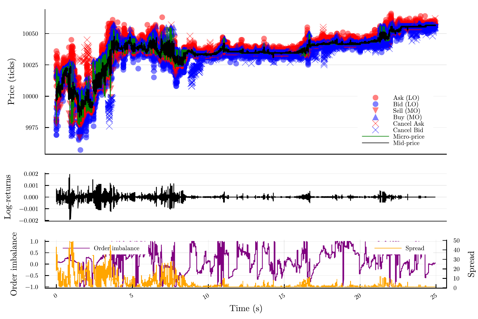
Figure 2: At the top of the figure is a 25 second (in machine time) simulated price path for the combined model configuration using a 6% ADV learning agent with a small state space (see Table 1). The environment is simulated using the calibrated parameters from Table 2. This is equivalent to a single trading day, i.e. 8 hours of typical trading in calendar time. The different markers and colours correspond to the different types of orders and the different sides of the LOB, respectively. The fluctuations in the log-micro-price returns, as well as the spread and order imbalance, are plotted in the middle and the bottom, respectively. These results visually demonstrate how the ABM and learning agent have produced well-known stylised facts. This is captured in more detail in Table 3 with further details in Supplementary Figures S1-8.

Learning agents

The learning agent explicitly changes the environment, necessitating a heuristic approach to demonstrate policy convergence. We visually show that we have reasonable policy convergence in the presence of Q-matrix difference stability and, furthermore, that the actions learnt are explicable, scaling as expected with the size of the parent order over multiple training episodes. This is visually shown in the supporting materials and reported in this paper. Figure 3 demonstrates that all the agents showed an improvement and convergence in profit over the episodes. From episodes 0 to approximately 250, there is an increase in the average profit and a decrease in the variance of the profit. After this period, the agents receive roughly the same profit when we ignore liquidity shocks of the agents with larger initial parent orders: $X_{0}$.

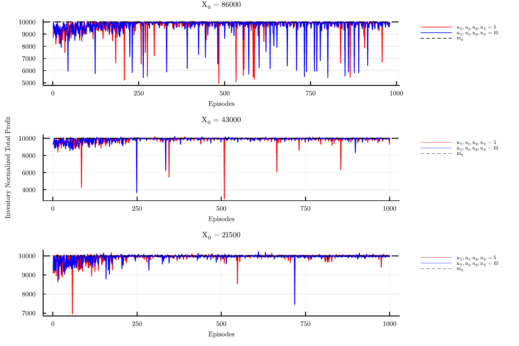
Figure 3: Plots the convergence in the profit of the RL agents. The amount of inventory the agent needed to trade increased from the bottom plot to the top plot. In each plot, we compare the profit convergence of the agents with smaller state space sizes to agents with larger state space sizes. $m_{0}$ is the initial mid-price, and if all agents were able to trade all shares at $m_{0}$ then the Inventory Normalised Total Profit (INTP) would be 10000, and the implementation shortfall would be 0. For the agents with the size of the parent order being 86000, the INTP was winsorised at the 1% and 99% levels to allow for easier comparisons. All agents demonstrate improvement and convergence in the profit. As the inventory increases, we start to see liquidity effects, as there are more frequent liquidity crashes. The size of the state space does not seem to cause significant differences in the profit, and all the agents were unable to significantly improve the profit received over the implementation shortfall amount.

As $X_{0}$ increases, the frequency of large price decreases and liquidity crashes increase – this is shown in Figure 5(b). Larger orders have a larger price impact and push the price further down. The impact of larger initial parent orders on the overall price impact is shown in Figure 7. Increasing the inventory traded will increase the chance of a large order being submitted, which can remove all the liquidity on the contra side of the order book before liquidity providers can replenish it, causing liquidity crashes.

There is no significant difference between the profit obtained by the smaller state space agents and the larger state space agents when they are trading the same amount of initial inventory. The difference between the number of states visited by the smaller and the larger state space agents is shown in Figure 4. Agents cannot significantly improve the profit received compared to if they could trade all inventory at the initial mid-price. The agents have learned to only reduce the implementation shortfall. Unsurprisingly, the smaller state space converges faster than the larger state space. The smaller state space also exhibits more jumps, likely due to the clustering of states. In particular, the more coarse-grained space would cause the agent to sample from one cluster and then jump to another, while the larger state space would have fewer distinct clusters, and the jumps between states would be less significant, giving a smoother convergence. Having far more states means that there will be fewer returns to individual states over the same number of episodes, which means the agents with the larger state space will likely have greater difficulty in learning a good policy over the same number of episodes.

The order volume trajectories learnt by the different agent configurations in the training environment are shown in Figure 5(a). The six different configurations are from Table 1. All the agents learned to execute more volume early in the trading session. There is more erratic trading for larger parent orders $X_{0}$ as the trading algorithm responds to larger volatility in the market states that actions respond to. The trading agent liquidating the larger parent order generates relatively more extreme events, as shown in Figure 5(b).

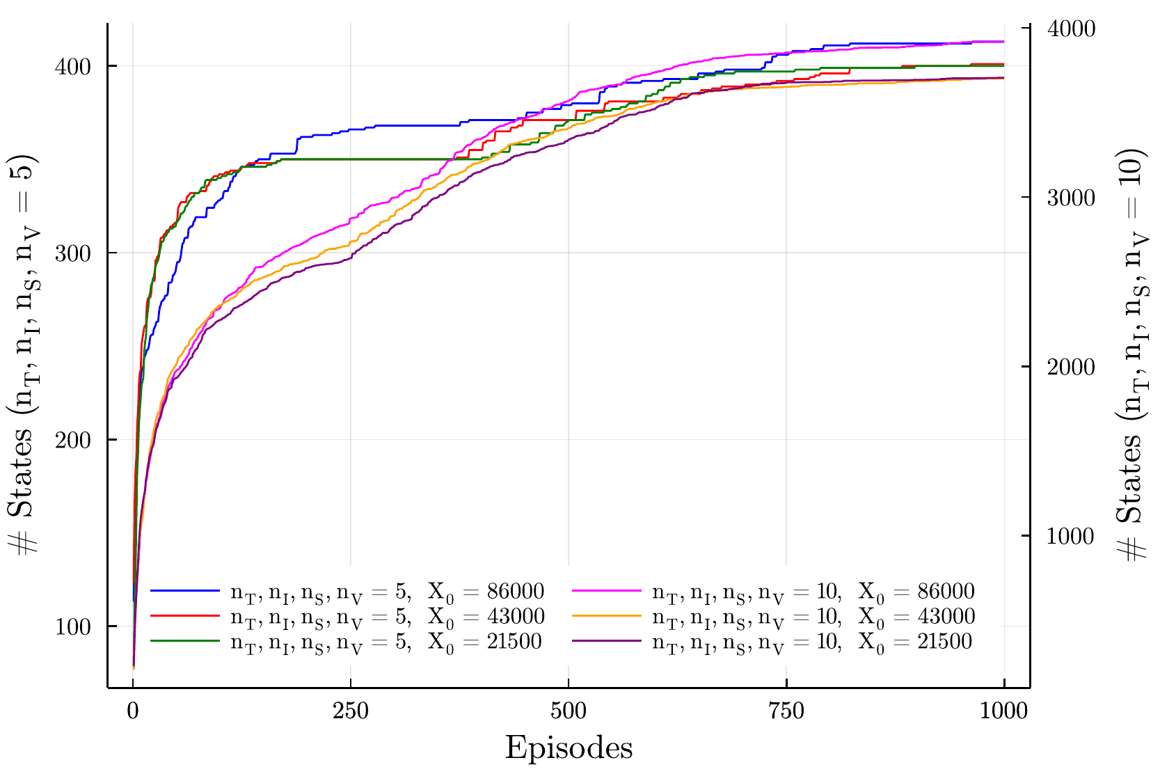
(a) Total number of Q-matrix states found

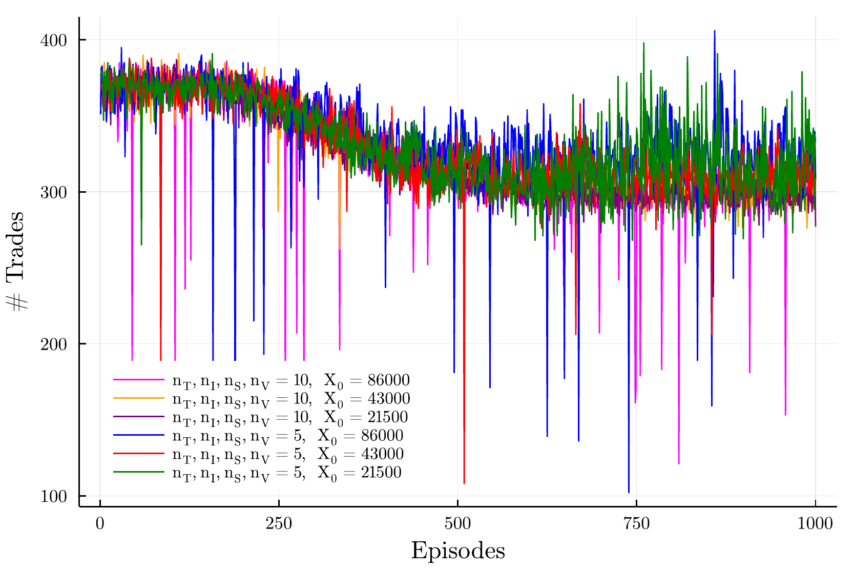
(b) The number of agent trade events

Figure 4: The total number of states found in the Q-matrix of each RL agent in each episode is shown on the left (Figure 4(a)). The smaller state space agents converge faster than the larger state space agents and have more jumps, whereas the larger state space agents exhibit a smoother convergence. The number of trade events an agent submits in each episode is plotted in Figure 4(b) and shows the decrease in the number of trades over the episodes and the convergence of this decrease.

Model stylised facts

It is difficult to assess the “goodness” of one ABM relative to another as most assessments are qualitative comparisons of stylised facts, and often, a variety of quite different ABMs can produce similar stylised facts. However, demonstrating the extent to which a calibrated model can reproduce the stylised facts of a market, and then that this is with relative stability, is a good starting point in validating an ABM, and it is a necessary step if one is to demonstrate the impact of model changes. We use the calibrated model and the associated moments estimated from the simulated samples to compare the different model configurations as the moments are changed in the presence of the learning agent.

The first stylised fact that will be considered is the fat-tails of the micro-price log-returns in event time. The ABM and the empirical returns were found to have fatter tails than that of the normal distribution, and the ABM was able to reproduce the stylised fact. Table 3 shows that the variance for the ABM is higher than what is observed in the market. The tails of the return distributions exhibited power-law or Pareto-like distributions with a tail-index that is finite [41, 25]. The ABM also has return distributions with near power-law behaviour in their tails. We found that the tail-index estimate for the simulated returns was less than the tail-index of the empirical returns, meaning there are fatter tails in the simulated return distribution; this is visualised across learning agent configurations in Figure 5(b) and was also observed in the moments in Table 3. Given that the distributions do not exactly follow a power-law, no conclusion about the existence of moments can be drawn from the tail-index parameter.

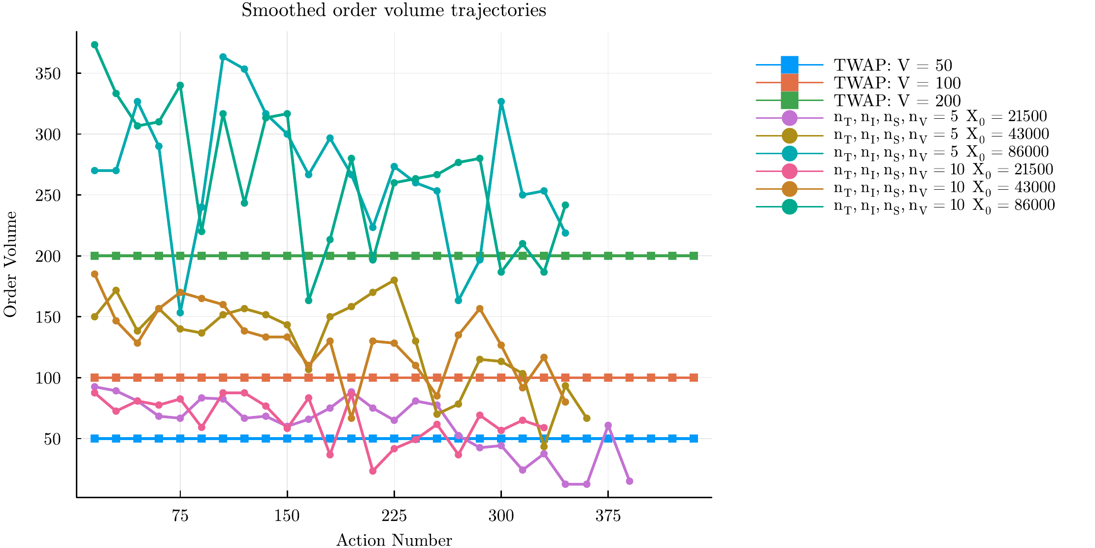
(a) Learning agent order volume trajectories

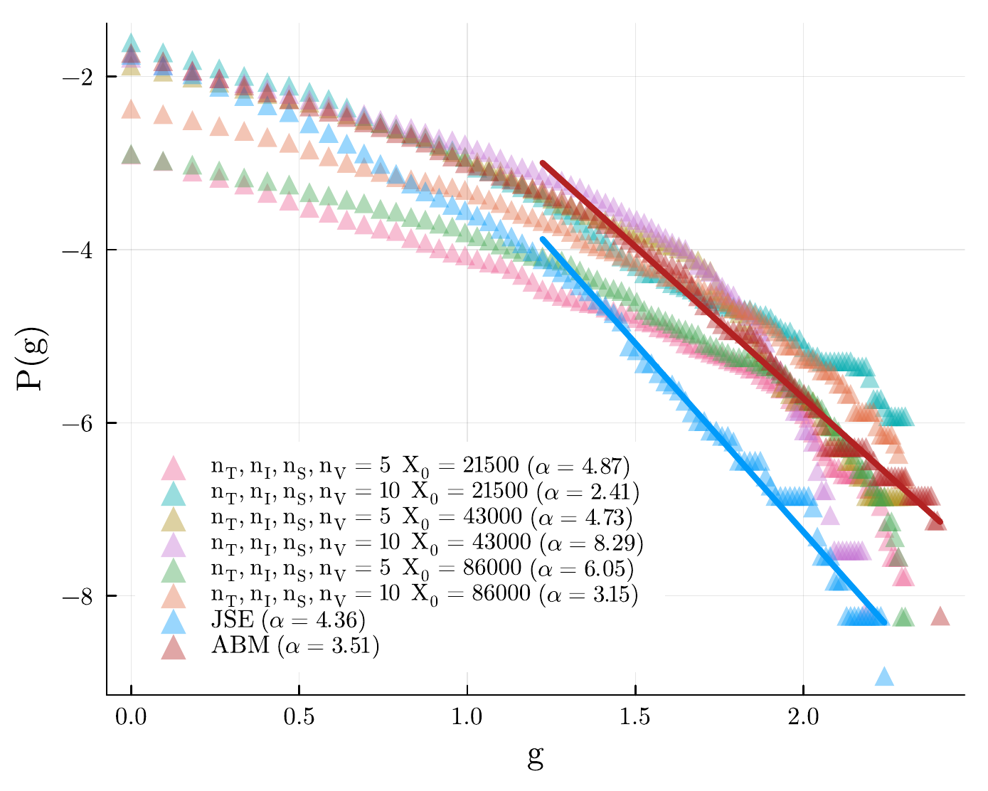
(b) The probability of exceedances

Figure 5: The order volume trading trajectories for the six different learning agent configurations are in Figure 5(a) (left). $X_{0}$ is the initial parent order. The TWAP for each of the three different initial order volumes is shown. V is the lot size. The trading agents have learnt to trade more early in the session and less later. The larger state spaces (10) are more erratic than the smaller ones (5). Agents with larger initial parent orders have more erratic trajectories. The associated changes in the exceedance probabilities are in Figure 5(b) (right), where $\alpha$ is the slope in the tail [25]. The exceedance probabilities for the ABM environment (red) are shown with a best-fit line in the linear region; similar plots are shown for the JSE (blue). The ABM has a higher number of extreme events due to liquidity shocks.

At high-frequency times scales, we have significant negative autocorrelations for the first lags, and the autocorrelations for the remaining lags are insignificant. This has been cited as evidence of a mean-reverting component of the time series that could potentially be attributed to market making [12]. We found significant negative autocorrelations for the first few lags where the autocorrelation in the simulated returns is far higher than the empirical returns, which may result from the frequency of limit orders placed by the high-frequency agents in the ABM. This is consistent with the estimated moments as the Hurst exponent in Table 3 suggests more mean-reversion in the simulated returns. Volatility clustering is the feature where large (resp. small) price variations are followed by further large (resp. small) price variations. This feature was calibrated using the GPH statistic, which measures the long-range dependence in the absolute log-returns. However, we found that the decay in the autocorrelations is far quicker for the simulated returns. Trade-signs have been shown to have persistence in their autocorrelations [39, 9, 53], meaning that buy (resp. sell) orders are followed by more buy (resp. sell) orders. To estimate the autocorrelation of the trade-signs each trade needs to be classified as a buy (+1) or a sell (-1). We use the Lee and Ready classification rules [38]. We then find that the model’s autocorrelation function (ACF) does not exhibit the same behaviour found in the empirical data. The ABM has captured the decay of the ACF for increasing lags. However, this decay is slower than the decay of the ACF for the empirical data. The model does reproduce the decay of the order-flow autocorrelation for increasing lags, but the volatility clustering effect is too strong, and it does not correctly describe the power-law decay seen in real markets. This only partially matches what is observed in the empirical data used to calibrate the ABM. This is not unexpected and was by design as made clear in the model discussion.

The impact of the different approach to time can be seen by comparing the stylised facts generated by the event-based reactive model, where there is no globally imposed model time, with those of the hybrid model, where there is a global time; these are otherwise the same models. Both models were able to reproduce the fat-tailed return distributions. However, one limitation of the hybrid model that has been resolved in our model is that the simulated returns have data more evenly distributed from the mean and less concentrated near zero. This also means that there is a smaller discrepancy between the tail-index estimates for the extreme-value distributions of the log-returns. The event-based ABM also captures that only the first few lags should be significantly negative, whereas significant lags (both positive and negative) up to lags of fifty were reported [32] in the hybrid model. The hybrid model’s decay in the absolute log-returns is faster than what is observed in our model. This means there is a weaker volatility clustering effect in the hybrid model.

However, the hybrid model can more accurately depict the decay in the trade-sign autocorrelation. In both these models, the order-flow autocorrelation is due to the herding effect caused by the chartists. We have changed the chartist rule to better suit event-driven activations without knowledge of a global calendar time. In contrast, in the hybrid model, the agent specification rule may better capture this feature because it is defined in the stochastic time setting. The selection of a global time is a potential source of top-down causation in the hybrid model that is not present in the reactive model. The chartists are more likely to be trading in events that are very close together, while in the hybrid model, stochastic time provides an external feature that spreads events away from event clusters. This can increase the herding effect seen in the event-based model. It must be noted that, for the hybrid mode, the trade-sign autocorrelation was not tested for the long-memory property. This means that even if the hybrid models better capture the decay, it is unclear if it indicates a long-memory process. Both models could accurately recover the depth profiles and price impact curves.

Conclusions

A reactive event-based ABM representing a trading environment was built using two classes of agents: liquidity takers who only submit market orders, and liquidity suppliers who only submit limit orders. The liquidity takers were split in turn into two sub-classes: fundamentalists and chartists. The fundamentalist started each trading session, such as a trading day, with different notions of fair or fundamental value, and traded accordingly. At the same time, the chartists considered a moving average of past price changes to trigger trading decisions. The ABM was implemented in event time using a reactive framework, so we did not need to specify at what calendar times agent activations could occur. Agents responded to events, not times. This simulated model for the environment recovers an asymmetry between the bid and ask depth profile curves, and both curves exhibit a rapid decrease in liquidity as the price moves away from the best bid/ask, remaining consistent with empirical observation [10, 26, 51]. The maximum volume at the best bid/ask is also consistent with previous research [51]. The simulated trading environment was calibrated to real-world data.

The real market observations were based on trade and order-book data extracted from the Johannesburg Stock Exchange (JSE) [33, 32] for a day of trading. The ABM representing the learning environment was calibrated using a simulated method of moments and calibrated parameters are provided in Table 2. This method of calibration was chosen to balance computational speed with stability. We found that the most significant parameters are the variance in the fundamental value $\sigma_{f}$, the intensity of the HFT order placement $\kappa$ and the number of chartist liquidity takers $N^{c}_{{}_{\mathrm{LT}}}$. Of lesser importance is the shape of the order-imbalance $\nu$, the number of fundamental liquidity takers $N^{f}_{{}_{\mathrm{LT}}}$ and the mid-price cut-off that sets the minimum volume lot sizes $\delta$. The model can recover log-returns that exhibit fat-tails with extreme value distributions similar to those observed in the market, with volatility clustering, and replicating the log-returns’ ACF. The ABM also captured the decay in the auto-correlation of the trade-signs, but with a slower decay rate when compared with the JSE. The JSE exhibited the expected long-memory property [39]. However, this was not fully replicated by the ABM. The decay of the auto-correlation in the absolute values of the log-returns was slower in the real market than in the ABM.

After the calibration of the training environment, a single learning agent with bounded rationality was added to the market to interact with this ABM. The learning agent was represented by a simple tabular Q-learning RL algorithm that was learning to solve an optimal execution selling problem using only market orders. This RL agent learns how to modify an existing TWAP trading schedule to optimally execute its sell order. The algorithm considered two market states based on features representing the limit-order book: the spread and the best bid volume, and then two states representing the current execution agents states: the remaining time available in the trading session, and the agents remaining inventory. The agent was tested with different parent order sizes and different state space sizes to observe whether any agents’ profits could be found to increase and converge and improve a random initial agent configuration. Our work shows that it can.

The impact of the different learning agent configurations on the environment is visually demonstrated in Figure 6 and Figure 5. In Figure 6, we see that the learning agents can suppress the trade-sign autocorrelations but boost the autocorrelations in the absolute micro-price value. This depends on the state space used in the learning algorithm, but learning agents with larger parent orders suppress the trade-sign autocorrelations and introduce more price volatility. Figure 7 shows that the larger parent orders induce a larger overall price impact even when the learning agent only engages in selling. The learnt volume trajectories for the different agents are shown in Figure 5(a) and their associated exceedance probabilities in Figure 5(b).

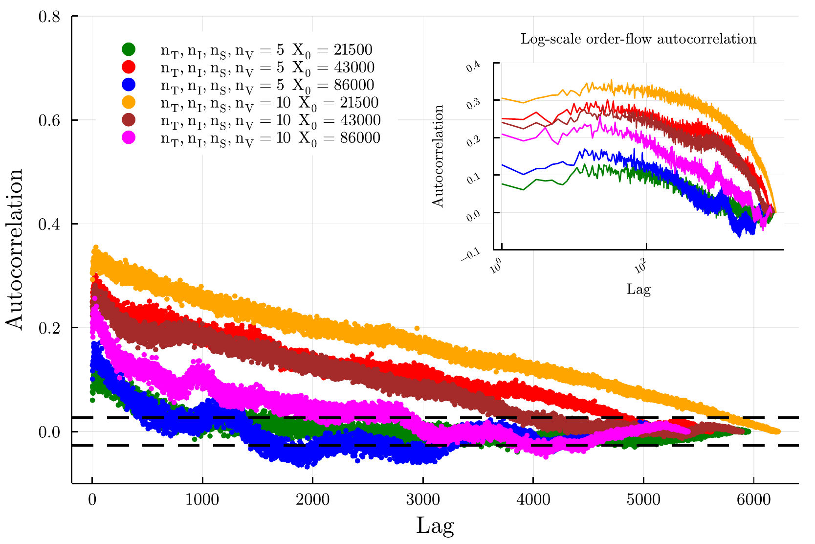
(a) Trade-sign autocorrelations

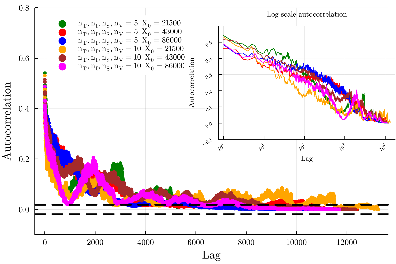
(b) Absolute return autocorrelations

Figure 6: The trade-sign autocorrelation plots for the ABM with the different RL agents are shown in Figure 6(a) and the autocorrelations in the absolute log-returns are in Figure 6(b). The state space sizes and initial inventories are given in the legend. Adding a learning agent using order-splitting does not guarantee the correct decay in the trade-sign autocorrelation. Agents plotted in green, blue and pink in Figure 6(a) show that these agents can reduce the trade-sign autocorrelations. These same agents can boost the autocorrelation in the absolute returns as seen for the agents plotted in green, blue and pink in Figure 6(b).

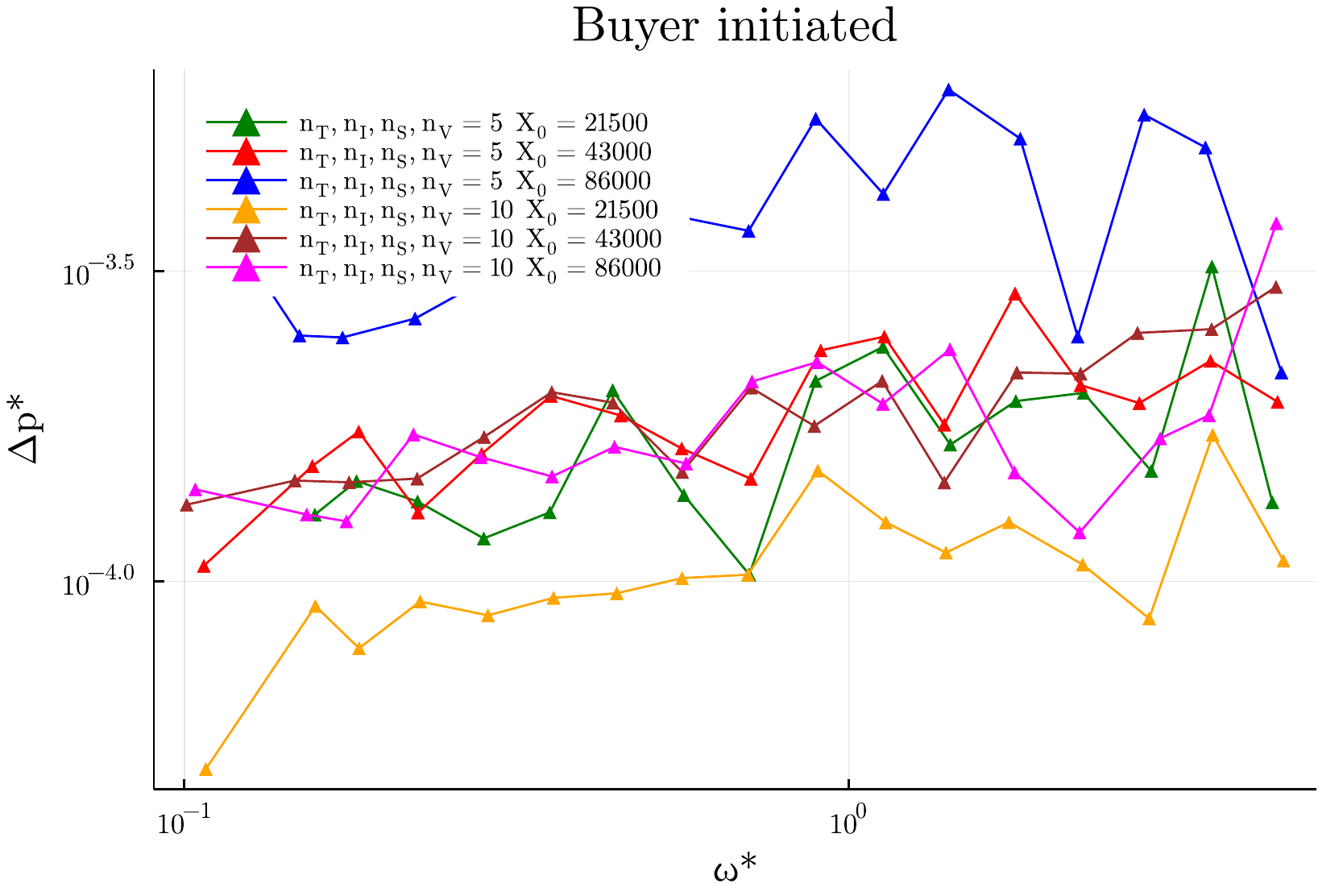
(a) Buyer initiated price impact

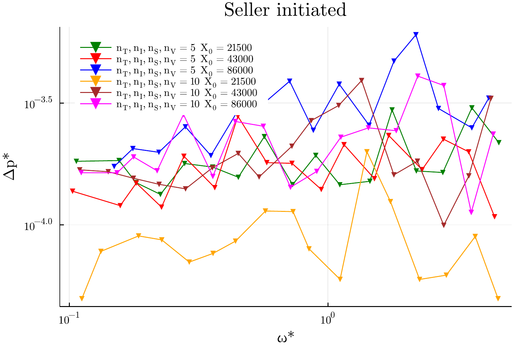
(b) Seller initiated price impact

Figure 7: Plots the price impact curves for the ABMs that include the RL agents, for buyer initiated (Figure 7(a)) and seller initiated (Figure 7(b)) trades. The linear upward trend in the price impact on the log-log scale indicates a power-law price impact function, where the price impact increases with the trade volume. Adding in the RL agents does not change the slope of the impact function. The observed price impact increases as the inventory traded increases and these price impact curves remain consistent with previous research [27, 31, 40, 32].

We compared the ABM representing the environment using its calibrated moments against the combination of the same ABM with a single strategic learning agent. We found that, except for the Hurst exponent, the moments were robust to adding a single simple learning agent, even with increasing initial order sizes. The combined market stylised facts conform to those observed in the measured market data. In particular, the combined model is found to better replicate the trade-sign and return absolute value autocorrelations, and these are shown in Figure 6. The model can replicate price impact functions with the correct shape, and an intuitive relationship with initial order sizes, as evidenced in Figure 7. When we include learning agents in the market environment, we can replicate the observed stylised facts better.

It was found that all agents could increase the profits over their initial random agent, demonstrating that each agent has learned. This is shown in Figure 3. However, an upper bound on the profits was observed. No agent could learn how to improve upon the profit of immediate execution (assuming that the execution volume was available). This shows that although the agents could reduce the implementation shortfall, they could not increase profits enough to observe a consistent and significant negative implementation shortfall. This is considered to be the result of the very simple reward function used. It was found that adding RL agents with increasing order sizes caused the ABM to have significant liquidity effects, as expected.

There were clear differences in the dynamics for agents with different state space sizes. The smaller state space agents had the number of states it visited converge much faster than the larger ones. They quickly finished the state discovery process while the larger state space agents were still rapidly discovering new states, limiting their learning ability. The larger state space agents showed less switching of actions in each state when compared with the small state space agents due to the agents not returning to individual states as often to update their state-action values.

This showed that the larger state space agents had difficulty learning in such few episodes. This was also evident in the behaviour learned. If a large state space agent had a large amount of inventory at the beginning of the simulation versus a smaller amount at the end, the agent did not learn to change behaviour while the smaller state space agent learned to trade more initially and then reduce the rate of trading at the end. There was also evidence that the smaller state space agent could learn to trade intuitively using the spread and volume states. Figure 4(b) shows that all agents learned to reduce the number of trades and guarantee the execution of the entire inventory. They also learned some structure during the training process, as evidenced by observed changes in the action volume trajectories over the training period.

This work promotes the idea there is value in combining minimally intelligent ABMs of the environment with the training of learning agents. We demonstrate that learning is feasible with trading agents comparable to those seen in real markets and that the combined model can generate relatively realistic market dynamics. From a market modelling perspective, we show that with strategic order-splitting, when combined with learning, we can more easily recover the observed auto-correlations of trade-signs and the auto-correlations of the absolute of the micro-prices while retaining realistic volume profiles, price impact profiles, and exceedance probabilities. Learning agents engaging in strategic order-splitting can suppress trade-sign auto-correlations, boost volatility, and increase mean-reversion effects.

Code and Data Availability

The JSE data used in this study is available at the ZivaHub repository, [33] 10.25375/uct.13187591.v1. The code used to implement the model management system is available at the ZivaHub repository, [15] 10.25375/uct.21163723.v1, and the matching engine with the UDP socket is available at the ZivaHub repository, [35] 10.25375/uct.21163993.v1

Reproducibility of the Research

The Julia code can be found in our GitHub site [15].

Author contributions statement

T.G. and M.D. conceived the experiments and models, M.D. implemented and conducted the experiments, T.G., A.P. and M.D. analysed the results and reformulated the experiments as required. All authors reviewed the manuscript.

References

- Almgren and Chriss [2001] Almgren, R., Chriss, N., 2001. Optimal execution of portfolio transactions. Journal of Risk 3, 5–40. doi:10.21314/JOR.2001.041.
- Aloud et al. [2017] Aloud, M., Fasli, M., Tsang, E., Dupuis, A., Olsen, R., 2017. Modeling the high-frequency fx market: An agent-based approach. Computational Intelligence 33, 771–825. doi:10.1111/coin.12114.
- Auletta et al. [2008] Auletta, G., Ellis, G.F.R., Jaeger, L., 2008. Top-down causation by information control: from a philosophical problem to a scientific research program. J. R. Soc. Interface , 1159–1172URL: https://royalsocietypublishing.org/doi/10.1098/rsif.2008.0018, doi:https://doi.org/10.1098/rsif.2008.0018.
- Barto and Mahadevan [2003] Barto, A.G., Mahadevan, S., 2003. Recent advances in hierarchical reinforcement learning. Discrete event dynamic systems 13, 41–77. doi:10.1023/A:1022140919877.
- Bellman [1954] Bellman, R., 1954. The theory of dynamic programming. Bulletin of the American Mathematical Society 60, 503–515. doi:10.1090/S0002-9904-1954-09848-8.
- Bertsimas and Lo [1998] Bertsimas, D., Lo, A.W., 1998. Optimal control of execution costs. Journal of Financial Markets 1, 1–50. doi:10.1016/S1386-4181(97)00012-8.
- Bezanson et al. [2021] Bezanson, J., Edelman, A., Karpinski, S., Shah, V.B., 2021. The Julia Programming Language. URL: https://julialang.org/. accessed: 2021-07-27.
- biasLab [2022] biasLab, 2022. Rocket.jl Documentation. URL: https://biaslab.github.io/Rocket.jl/stable/. biasLab/Rocket.jl v1.4.0. Accessed: 2022-09-09.
- Bouchaud et al. [2003] Bouchaud, J.P., Gefen, Y., Potters, M., Wyart, M., 2003. Fluctuations and response in financial markets: the subtle nature ofrandom’price changes. Quantitative finance 4, 176. doi:10.1080/14697680400000022.
- Bouchaud et al. [2002] Bouchaud, J.P., Mézard, M., Potters, M., 2002. Statistical properties of stock order books: empirical results and models. Quantitative finance 2, 251–256. doi:10.1088/1469-7688/2/4/301.
- Cartea et al. [2015] Cartea, Á., Jaimungal, S., Penalva, J., 2015. Algorithmic and high-frequency trading. Cambridge University Press.
- Cont [2001] Cont, R., 2001. Empirical properties of asset returns: stylized facts and statistical issues. Quantitative Finance 1, 223–236. doi:10.1080/713665670.
- Crafa [2021] Crafa, S., 2021. From agent-based modeling to actor-based reactive systems in the analysis of financial networks. Journal of Economic Interaction and Coordination 16, 649–673. URL: https://doi.org/10.1007/s11403-021-00323-8, doi:10.1007/s11403-021-00323-8.
- Dickey and Fuller [1979] Dickey, D.A., Fuller, W.A., 1979. Distribution of the estimators for autoregressive time series with a unit root. Journal of the American Statistical Association 74, 427–431. doi:10.1080/01621459.1979.10482531.
- Dicks and Gebbie [2022] Dicks, M., Gebbie, T., 2022. A simple learning agent interacting with an agent-based market model: Julia code. figshare URL: https://zivahub.uct.ac.za/articles/software/A_simple_learning_agent_interacting_with_an_agent-based_market_model_Julia_code/21163723, doi:{10.25375/uct.21163723.v1}.
- Dicks et al. [2023] Dicks, M., Paskaramoothy, A., Gebbie, T., 2023. Many learning agents interacting with an agent-based market model. arXiv:2303.07393.
- Dieci and He [2018] Dieci, R., He, X.Z., 2018. Heterogeneous agent models in finance. Handbook of computational economics 4, 257–328. URL: https://www.sciencedirect.com/science/article/pii/S157400211830008X, doi:10.1016/bs.hescom.2018.03.002.
- Fabretti [2013] Fabretti, A., 2013. On the problem of calibrating an agent based model for financial markets. Journal of Economic Interaction and Coordination 8, 277–293. doi:10.1007/s11403-012-0096-3.
- Farmer et al. [2005] Farmer, J.D., Patelli, P., Zovko, I.I., 2005. The predictive power of zero intelligence in financial markets. Proceedings of the National Academy of Sciences 102, 2254–2259. URL: https://www.pnas.org/content/102/6/2254, doi:10.1073/pnas.0409157102.
- Gao and Han [2012] Gao, F., Han, L., 2012. Implementing the nelder-mead simplex algorithm with adaptive parameters. Computational Optimization and Applications 51, 259–277. doi:10.1007/s10589-010-9329-3.
- Garcia and Ndiaye [1998] Garcia, F., Ndiaye, S.M., 1998. A learning rate analysis of reinforcement learning algorithms in finite-horizon, in: ICML ’98: Proceedings of the Fifteenth International Conference on Machine Learning, Morgan Kaufmann Publishers Inc., San Francisco, CA, USA. pp. 215–223.
- Geweke and Porter-Hudak [1983] Geweke, J., Porter-Hudak, S., 1983. The estimation and application of long memory time series models. Journal of time series analysis 4, 221–238. doi:10.1111/j.1467-9892.1983.tb00371.x.
- Gilles [2006] Gilles, D., 2006. Asynchronous simulations of a limit order book. Master’s thesis. University of Manchester.
- Gilli and Winker [2003] Gilli, M., Winker, P., 2003. A global optimization heuristic for estimating agent based models. Computational Statistics & Data Analysis 42, 299–312. doi:10.1016/S0167-9473(02)00214-1.
- Gopikrishnan et al. [1998] Gopikrishnan, P., Meyer, M., Amaral, L.A.N., Stanley, H., 1998. Inverse cubic law for the distribution of stock price variations. Eur. Phys. J. B 3, 139–140. doi:https://doi.org/10.1007/s100510050292.
- Gould et al. [2013] Gould, M.D., Porter, M.A., Williams, S., McDonald, M., Fenn, D.J., Howison, S.D., 2013. Limit order books. Quantitative Finance 13, 1709–1742. doi:10.1080/14697688.2013.803148.
- Harvey et al. [2016] Harvey, M., Hendricks, D., Gebbie, T., Wilcox, D., 2016. Deviations in expected price impact for small transaction volumes under fee restructuring. Physica A: Statistical Mechanics and its Applications 471, 416–426. doi:10.1016/j.physa.2016.11.042.
- Hendricks and Wilcox [2014] Hendricks, D., Wilcox, D., 2014. A reinforcement learning extension to the almgren-chriss framework for optimal trade execution, in: 2014 IEEE Conference on Computational Intelligence for Financial Engineering & Economics (CIFEr), IEEE. pp. 457–464. doi:10.1109/CIFEr.2014.6924109.
- Hewitt [2011] Hewitt, C., 2011. Actor model of computation: Scalable robust information systems. Proceedings of Inconsistency Robustness, Stanford .
- Hurst [1951] Hurst, H.E., 1951. Long-term storage capacity of reservoirs. Transactions of the American Society of Civil Engineers 116, 770–799. doi:10.1061/TACEAT.0006518.
- Jericevich et al. [2020a] Jericevich, I., Chang, P., Gebbie, T., 2020a. Comparing the market microstructure between two South African exchanges. arXiv:2011.04367.
- Jericevich et al. [2021] Jericevich, I., Chang, P., Gebbie, T., 2021. Simulation and estimation of an agent-based market-model with a matching engine. arXiv:2108.07806.
- Jericevich et al. [2020b] Jericevich, I., Chang, P., Pillay, A., Gebbie, T., 2020b. Supporting test data: Comparing the market microstructure between two south african exchanges. URL: https://zivahub.uct.ac.za/articles/dataset/Supporting_Test_Data_Comparing_the_Market_Microstructure_Between_two_South_African_Exchanges/13187591, doi:10.25375/uct.13187591.v1.
- Jericevich et al. [2022a] Jericevich, I., Sing, D., Gebbie, T., 2022a. Cointossx: An open-source low-latency high-throughput matching engine. SoftwareX 19, 101136. URL: https://www.softxjournal.com/article/S2352-7110(22)00087-5/pdf, doi:10.1016/j.softx.2022.101136.
- Jericevich et al. [2022b] Jericevich, I., Sing, D., Gebbie, T., Dicks, M., 2022b. CoinTossX with market data feed. figshare URL: https://zivahub.uct.ac.za/articles/software/CoinTossX_with_market_data_feed/21163993, doi:10.25375/uct.21163993.v1.
- Leal et al. [2016] Leal, S.J., Napoletano, M., Roventini, A., Fagiolo, G., 2016. Rock around the clock: An agent-based model of low-and high-frequency trading. Journal of Evolutionary Economics 26, 49–76.
- LeBaron [2000] LeBaron, B., 2000. Agent-based computational finance: Suggested readings and early research. Journal of Economic Dynamics and Control 24, 679–702. URL: https://www.sciencedirect.com/science/article/pii/S0165188999000226, doi:10.1016/S0165-1889(99)00022-6.
- Lee and Ready [1991] Lee, C.M.C., Ready, M.J., 1991. Inferring trade direction from intraday data. The Journal of Finance 46, 733–746. doi:10.1111/j.1540-6261.1991.tb02683.x.
- Lillo and Farmer [2007] Lillo, F., Farmer, J.D., 2007. The long memory of the efficient market. Studies in Nonlinear Dynamics & Econometrics 8, 1–1. doi:10.2202/1558-3708.1226.
- Lillo et al. [2003] Lillo, F., Farmer, J.D., Mantegna, R., 2003. Master curve for price-impact function. Nature 421, 129–30. doi:10.1038/421129a.
- Mandelbrot [1963] Mandelbrot, B.B., 1963. The variation of certain speculative prices. The Journal of Business 36, 394–419. URL: http://www.jstor.org/stable/2350970.
- Mandelbrot and Wallis [1969] Mandelbrot, B.B., Wallis, J.R., 1969. Robustness of the rescaled range r/s in the measurement of noncyclic long run statistical dependence. Water Resources Research 5, 967–988. doi:https://doi.org/10.1029/WR005i005p00967.
- Mandeş [2015] Mandeş, A., 2015. Microstructure-based order placement in a continuous double auction agent based model. Algorithmic Finance 4, 105–125. doi:10.3233/AF-150049.
- Mandeş and Winker [2017] Mandeş, A., Winker, P., 2017. Complexity and model comparison in agent based modeling of financial markets. Journal of Economic Interaction and Coordination 12, 469–506. doi:10.1007/s11403-016-0173-0.
- Massey [1951] Massey, F.J.J., 1951. The kolmogorov-smirnov test for goodness of fit. Journal of the American Statistical Association 46, 68–78. doi:10.1080/01621459.1951.10500769.
- Nuyts [2010] Nuyts, J., 2010. Inference about the tail of a distribution: Improvement on the hill estimator. International Journal of mathematics and mathematical sciences 2010. doi:10.1155/2010/924013.
- Obizhaeva and Wang [2013] Obizhaeva, A.A., Wang, J., 2013. Optimal trading strategy and supply/demand dynamics. Journal of Financial Markets 16, 1–32. doi:10.1016/j.finmar.2012.09.001.
- Platt [2020] Platt, D., 2020. A comparison of economic agent-based model calibration methods. Journal of Economic Dynamics and Control 113, 103859. URL: https://www.sciencedirect.com/science/article/pii/S0165188920300294, doi:10.1016/j.jedc.2020.103859.
- Platt and Gebbie [2016] Platt, D., Gebbie, T., 2016. The problem of calibrating an agent-based model of high-frequency trading. arXiv:1606.01495.
- Platt and Gebbie [2018] Platt, D., Gebbie, T., 2018. Can agent-based models probe market microstructure? Physica A: Statistical Mechanics and its Applications 503, 1092–1106. URL: https://www.sciencedirect.com/science/article/pii/S0378437118309956, doi:10.1016/j.physa.2018.08.055.
- Potters and Bouchaud [2003] Potters, M., Bouchaud, J.P., 2003. More statistical properties of order books and price impact. Physica A: Statistical Mechanics and its Applications 324, 133–140. doi:10.1016/S0378-4371(02)01896-4.
- Sutton and Barto [2018] Sutton, R.S., Barto, A.G., 2018. Reinforcement learning: An introduction. MIT press.
- Toth et al. [2015] Toth, B., Palit, I., Lillo, F., Farmer, J.D., 2015. Why is equity order flow so persistent? Journal of Economic Dynamics and Control 51, 218–239. doi:10.1016/j.jedc.2014.10.007.
- Watkins and Dayan [1992] Watkins, C.J., Dayan, P., 1992. Q-learning. Machine learning 8, 279–292. doi:10.1007/BF00992698.
- Watkins [1989] Watkins, C.J.C.H., 1989. Learning from delayed rewards. Ph.D. thesis. King’s College, Cambridge United Kingdom.
- Wilcox and Gebbie [2014] Wilcox, D., Gebbie, T., 2014. Hierarchical causality in financial economics. Available at SSRN: URL: https://ssrn.com/abstract=2544327, doi:http://dx.doi.org/10.2139/ssrn.2544327.
- Winker et al. [2007] Winker, P., Gilli, M., Jeleskovic, V., 2007. An objective function for simulation based inference on exchange rate data. Journal of Economic Interaction and Coordination 2, 125–145. doi:10.1007/s11403-007-0020-4.