Compactifications of moduli spaces of K3 surfaces with a nonsymplectic involution

Abstract.

There are $75$ moduli spaces $F_{S}$ of K3 surfaces with a nonsymplectic involution. We give detailed descriptions of Kulikov models for one-parameter degenerations in $F_{S}$. In the $50$ cases where the fixed locus of the involution has a component $C_{g}$ of genus $g\geq 2$, we identify normalizations of the KSBA compactifications of $F_{S}$ via stable pairs $(X,\epsilon C_{g})$, with explicit semitoroidal compactifications of $F_{S}$.

1. Introduction

Let $X$ be a smooth projective K3 surface. An involution $\iota$ of $X$ is called nonsymplectic if it acts as $\iota^{*}\omega_{X}=-\omega_{X}$ on a generator of $H^{2,0}(X)$. The $(+1)$-eigenspace of the induced involution on $H^{2}(X,{\mathbb{Z}})$ is a hyperbolic lattice $S$. All the possibilities for $S$ were found in a classical work [Nik79a] of Nikulin, who proved that there are $75$ cases, given in Fig. 1. The lattices $S$ are uniquely determined by a triple of invariants $(r,a,\delta)$, or an equivalent set of invariants, $(g,k,\delta)$.

For a given lattice $S$, there is a moduli space $F_{S}$ of K3 surfaces with an involution and generic Picard lattice $S$. It is an open subset of ${\mathbb{D}}_{S}/\Gamma$, the quotient of a type IV domain of dimension $20-\operatorname{rank}S$ by an arithmetic group.

The K3 surfaces that appear include many interesting ones, for example the double covers of: Enriques surfaces, smooth del Pezzo surfaces, log del Pezzo surfaces of index $2$, index $2$ Halphen pencils, and rational elliptic surfaces. They have been the subject of a great deal of research. Here, we are interested in geometric compactifications of the moduli spaces $F_{S}$.

In $50$ of the $75$ cases, the fixed locus $R$ of the involution contains a smooth curve $C_{g}$ of genus $g\geq 2$. The divisor $C_{g}$ is semiample and defines a contraction $X\to{\overline{X}}$ to a K3 surface with $ADE$ singularities and an ample Cartier divisor ${\overline{C}}_{g}$.

It follows that for $0<\epsilon\ll 1$ the pair $({\overline{X}},\epsilon{\overline{C}}_{g})$ is a KSBA stable pair, see [Kol23] for their general theory. Stable pairs have complete, projective moduli spaces. One thus obtains a geometrically meaningful KSBA compactification ${\overline{F}}_{S}$.

Problem 1.1.

Describe the compactification ${\overline{F}}_{S}$ explicitly.

In previous collaborations, we solved this problem in two cases: for the degree 2 K3 surfaces [AET19] and for the elliptic degree 2 K3 surfaces [ABE22], which is a Heegner divisor in the previous case. In this paper, we solve it for all the remaining cases:

Theorem 1.2.

The normalization of ${\overline{F}}_{S}$ is a semitoroidal compactification of ${\mathbb{D}}_{S}/\Gamma$ for an explicit semifan ${\mathfrak{F}}_{\rm ram}$. In $48$ of the $50$ cases it is dominated by a toroidal compactification for a Coxeter reflection fan.

The precise statement is given in Theorem 9.10. We reduce Problem 1.1 to the following problem which we solve for all $75$ cases:

Problem 1.3.

For each cusp of the Baily-Borel compactification ${\overline{F}}_{S}^{\rm BB}$ and each one-parameter degeneration $C\setminus 0\to F_{S}$ approaching that cusp, describe explicitly a Kulikov model $X\to(C,0)$ adapted to the ramification divisor $R$.

A Kulikov model is a $K$-trivial SNC model $X\to(C,0)$ with smooth total space, and it is adapted to $R$ if $R_{t}\subset X_{t}$ for $t\in C\setminus 0$ extends to $X_{0}$ as a divisor not containing singular strata, and the limit of any component of positive genus is nef.

The answer to the last problem can be read off directly from the Coxeter diagrams of the reflection groups of the hyperbolic lattices ${\overline{T}}$ appearing at the $0$-cusps of $F_{S}$. The reason for this is quite simple. The main tool we use is the mirror symmetry between degenerations in the $S$-family and nef line bundles on mirror K3 surfaces ${\widehat{X}}$ with Picard lattice ${\widehat{S}}={\overline{T}}$. The nef cone of a K3 surface depends on, and is described by the reflection group of its Picard lattice.

The structure of the paper is as follows. In Section 2 we recall the theory of K3 surfaces with a nonsymplectic involution, of $2$-elementary lattices, and the general facts about the moduli spaces $F_{S}$ of K3 surfaces with group action. We also recall basic facts about the combinatorial (Baily-Borel, toroidal, semitoroidal) and functorial (KSBA) compactifications of these moduli spaces.

In Section 3 we recall Vinberg’s theory of reflection groups in hyperbolic spaces and the Coxeter-Vinberg diagrams. We don’t need the Coxeter groups for all the $75$ of the $2$-elementary lattices but only for those that appear at the $0$-cusps of $F_{S}$ for some $S$. These are the lattices with $g\geq 1$, excluding $(r,a,\delta)=(14,6,0)$. For the lattices with $g\geq 2$ the Coxeter diagrams were computed by Nikulin in [AN06]. A few cases on the $g=1$ line were previously known. We complete the job for the remaining lattices, the answer is given in Figs. 3 and 4.

In Section 4 we describe K3 surfaces appearing in the $75$ families, their quotients by the involution, and their nef cones. The $75$ families are woven together in a web by certain “Heegner divisor moves,” corresponding to when one moduli space $F_{S^{\prime}}$ is a Heegner divisor in or at the boundary of $F_{S}$. We describe these moves and their properties.

In Section 5 we completely describe the $0$- and $1$-cusps of $F_{S}$ together with the incidence relations between them. In particular, the $0$-cusps of $F_{S}$ are described by three kinds of “mirror moves” on the nodes of Fig. 1, making it into a directed graph in which every vertex has in- and out-degrees equal to $0$, $1$, $2$, or $3$.

In Section 6 we discuss the theory of integral-affine spheres ($\operatorname{IAS}^{2}$) in relation to Kulikov models. It is well known that the dual graph $\Gamma(X_{0})$ of a Type III Kulikov central fiber $X_{0}=\cup V_{i}$ is a triangulation of $S^{2}$. In simple terms, the integral affine sphere $B=\Gamma(X_{0})$ is an economical description for $X_{0}$. The singularities of the $\operatorname{IAS}^{2}$ describe the nontoric components $V_{i}$. The same integral-affine structures describe a Lagrangian torus fibration $\mu\colon{\widehat{X}}\to B$ on a mirror K3 surface ${\widehat{X}}$ with a symplectic form, e.g. given by an ample line bundle.

In Section 7 we study this mirror correspondence specifically for K3 surfaces with a nonsymplectic involution. To understand the Kähler geometry of $X$, encoded by the divisor $R$, we must understand the complex geometry of ${\widehat{X}}$. The key is a special degeneration of ${\widehat{X}}$ into two copies ${\widehat{X}}_{0}={\widehat{Y}}\cup{\widehat{Y}}$ of the surface ${\widehat{Y}}={\widehat{X}}/\hat{\iota}$, the quotient of ${\widehat{X}}$ by the mirror involution. This applies to all the cases except for the Enriques case, where the answer is even more interesting: ${\widehat{Y}}$ is an Halphen pencil, and the gluing is by a $2$-torsion twist on the multiple fiber.

The resulting $\operatorname{IAS}^{2}$ is of a particularly simple kind: $B=P\cup P^{\rm opp}$, the union of two isomorphic “hemispheres”, Symington polytopes for ${\widehat{Y}}$ glued along a circular equator representing an anticanonical boundary of ${\widehat{Y}}$. We prove that the mirror correspondence exchanges the $(\pm 1)$-eigenspaces on the lattices $H^{2}(X,{\mathbb{Z}})$, $H^{2}({\widehat{X}},{\mathbb{Z}})$ modulo the vanishing cycle, resp. the fiber class of the Lagrangian torus fibration.

In Section 8, for each lattice ${\overline{T}}$ appearing at a $0$-cusp of $F_{S}$, and each monodromy invariant $\lambda\in{\overline{T}}$ encoding the Picard-Lefschetz transform of a one-parameter degeneration, we construct explicitly the families of Kulikov surfaces with involution that appear, up to taking some multiple of $\lambda$.

In Section 9 we first define the semifans appearing in Theorem 1.2. Next, we compute the stable models for the Kulikov surfaces of Section 8. Finally, we prove Theorem 1.2 by applying the general theory of [AE21] and [AEH21].

Acknowledgements.

The authors were partially supported by the NSF grants DMS-2201222 and DMS-2201221 respectively.

2. K3 surfaces with involution and $2$-elementary lattices

2A. K3 surfaces with a nonsymplectic involution

Let $X$ be a smooth projective complex K3 surface. An involution $\iota$ of $X$ is called nonsymplectic if it acts as $\iota^{*}\omega_{X}=-\omega_{X}$ on a non-vanishing holomorphic two-form $\omega_{X}\in H^{2,0}(X)$. It is well known that the quotient $Y=X/\iota$ is either a rational or Enriques surface and that $X$ is algebraic.

The main invariant of the involution is the $(+1)$ eigenspace $S=H^{2}(X,{\mathbb{Z}})^{+}$, a hyperbolic lattice of some rank $r$. Its orthogonal complement $T=S^{\perp}=H^{2}(X,{\mathbb{Z}})^{-}$ in $H^{2}(X,{\mathbb{Z}})$ is a lattice of signature $(2,20-r)$. There is a canonical isomorphism $A_{S}=A_{T}$ between the discriminant lattices $A_{S}=S^{*}/S$ and $A_{T}=T^{*}/T$. The involution acts by multiplication by $\pm 1$ on $A_{S}$ and $A_{T}$ respectively. This implies that $A_{S}={\mathbb{Z}}_{2}^{a}$ for some $a\geq 0$. Such lattices are called $2$-elementary.

Conversely, if $S\subset L_{\rm K3}={\rm II}_{3,19}=U^{\oplus 3}\oplus E_{8}^{\oplus 2}$ is a primitive $2$-elementary lattice and $T=S^{\perp}$ then the involution $\rho$ of $L_{\rm K3}\otimes{\mathbb{Q}}$ acting as $\pm 1$ on $S$ and $T=S^{\perp}$ respectively is an involution of $L_{\rm K3}$. If $X$ is a K3 surface whose Picard lattice $S_{X}$ equals $S$ via some marking $H^{2}(X,{\mathbb{Z}})\to L_{\rm K3}$ then by the Torelli theorem, there exists a unique involution $\iota$ of $X$ such that $\iota^{*}=\rho$.

An indefinite even $2$-elementary lattice is uniquely determined by its signature and the triple $(r,a,\delta)=({\rm rk}_{{\mathbb{Z}}}S,\,{\rm rk}_{{\mathbb{Z}}_{2}}A_{S},\,\delta)$, where $\delta\in\{0,1\}$ is an additional invariant explained in the next section. The $2$-elementary hyperbolic lattices admitting a primitive embedding into $L_{\rm K3}$ were classified by Nikulin in [Nik79a, 3.6.2]. There are 75 lattices and for each of them, an embedding into $L_{\rm K3}$ is unique up to $O(L_{\rm K3})$. The result is given in Fig. 1.

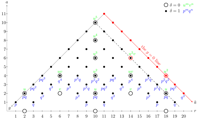
Figure 1. Hyperbolic $2$-elementary K3 lattices $(r,a,\delta)$

The fixed locus $R=X^{\iota}$ of the involution and the quotient surface $Y=X/\iota$ are smooth. Denote by $k+1$ the number of the irreducible components of $R$ and by $g$ the sum of their genera (excluding the special Enriques case). Then

(1) $$g=11-\tfrac{1}{2}(r+a)\text{ and }k=\tfrac{1}{2}(r-a)$$

and the triple $(g,k,\delta)$ is an alternative set of invariants of $S$. There are three cases:

1. $R$ is a union of a curve $C_{0}$ of genus $g\geq 0$ and $k$ additional curves $C_{1},\dotsc,C_{k}$ each isomorphic to ${\mathbb{P}}^{1}$. The surface $Y$ is rational.

2. $R=C_{0}\sqcup C_{1}$ is the union of two elliptic curves. Then $(r,a,\delta)=(10,8,0)$ and $(g,k,\delta)=(2,1,0)$. The surface $Y$ is rational elliptic.

3. $R=\emptyset$. Then $(r,a,\delta)=(10,10,0)$ and $(g,k,\delta)=(1,0,0)$. The surface $Y$ is Enriques.

Remark 2.1.

The case $(10,8,0)$ in many ways is more similar to those on the $g=1$ line than to those with $g\geq 2$. For example, the automorphism group of a K3 surface with this Picard lattice is infinite. Its Coxeter diagram, given in Fig. 3, is the same as for $(10,10,1)$. See also Theorem 4.1.

In the next sections, we briefly recall the theory of $2$-elementary lattices and two ways of constructing the moduli spaces of K3 surfaces with a nonsymplectic involution.

2B. $2$-elementary lattices

A lattice $H$ is a free finite rank ${\mathbb{Z}}$-module together with a nondegenerate ${\mathbb{Z}}$-valued bilinear form. It is called even if $x^{2}\equiv 0\pmod{2{\mathbb{Z}}}$ for all $x\in H$ and odd otherwise. The discriminant lattice is $A_{H}=H^{*}/H$, where $H^{*}\subset H_{\mathbb{Q}}$ is the dual lattice. It comes with the discriminant form $q_{H}\colon A_{H}\to{\mathbb{Q}}/{\mathbb{Z}}$, $q(x)=x^{2}$. Moreover, if $H$ is even then $q_{H}$ takes well-defined values in ${\mathbb{Q}}/2{\mathbb{Z}}$. One also has the associated bilinear form $b_{H}\colon A_{H}\times A_{H}\to{\mathbb{Q}}/{\mathbb{Z}}$.

If $L$ is a unimodular lattice, $S\subset L$ a primitive (i.e. saturated) sublattice and $T=S^{\perp}$ then $(A_{S},q_{S})=(A_{T},-q_{T})$ in a canonical way.

2.2.

If $S$ and $T$ are, respectively, the $(\pm 1)$-eigenspaces of an involution $\iota$ on $L$ then $\iota$ acts as identity on $A_{S}$ and as $(-1)$ on $A_{T}$. Therefore, $A_{S}\simeq{\mathbb{Z}}_{2}^{a}$ for some $a$. Lattices $H$ with $A_{H}\simeq{\mathbb{Z}}_{2}^{a}$ are called $2$-elementary. Thus, $S$ and $T$ are $2$-elementary in this case.

Definition 2.3.

We define an additional invariant, coparity $\delta_{H}$ as follows: $\delta=0$ if for all $x\in A_{H}$ one has $q_{H}(x)\equiv 0\pmod{{\mathbb{Z}}}$ and $\delta=1$ otherwise. We will call lattices with $\delta_{H}=0$ co-even and lattices with $\delta_{H}=1$ co-odd.

This notation is explained by the following. Recall that for any lattice $K$, $K(n)$ denotes the lattice with the bilinear product scaled by $n$, i.e. $(x,y)_{K(n)}=n\cdot(x,y)_{K}$.

Definition 2.4.

For a $2$-elementary (not necessarily even) lattice $H$, the doubled dual is $H^{\dagger}=H^{*}(2)$. The assignment $H\to H^{\dagger}$ is an involution since

$$(H^{\dagger})^{\dagger}=\left(H^{*}(2)\right)^{*}(2)=H(\tfrac{1}{2})(2)=H.$$

The doubled dual operation interchanges the parity and co-parity:

Lemma 2.5.

Let $H$ be a $2$-elementary lattice with invariants $(r,a,\delta)$. Then $H^{\dagger}$ is a $2$-elementary lattice of the same signature with invariants $(r,r-a,\delta^{\dagger})$ and the discriminant group is

$$A_{H^{\dagger}}=(H^{\dagger})^{*}/H^{\dagger}=H(\tfrac{1}{2})/H^{*}(2).$$

Moreover, $\delta=0$ (resp. $\delta=1$) iff $H^{\dagger}$ is even (resp. odd), and $H$ is even (resp. odd) iff $\delta^{\dagger}=0$ (resp. $\delta^{\dagger}=1$).

Proof.

For $x,y\in H^{*}$ one has $2x\in H$ so $(x,y)_{H^{\dagger}}=2(x,y)=(2x,y)\in{\mathbb{Z}}$. So $H^{\dagger}$ is indeed a ${\mathbb{Z}}$-lattice. The equation for the discriminant group is immediate. Since $H$ is $2$-elementary, one has

$$H\subset 2H^{*}\subset\tfrac{1}{2}H\implies 2H^{\dagger}=2H^{*}(2)\subset\tfrac{1}{2}H(2)=H(\tfrac{1}{2}),$$

so $H^{\dagger}$ is $2$-elementary of the same rank $r$, and the ${\mathbb{Z}}_{2}$-rank of the discriminant group is $2r-(r+a)=r-a$. For $x\in H^{*}$ one has $(x,x)_{H^{*}}=\frac{1}{2}(x,x)_{H^{\dagger}}$, so $\delta_{H}=0$ iff $H^{\dagger}$ is even. The last part holds by symmetry. ∎

We recall the following facts about $2$-elementary lattices proved in [Nik79a]. Any indefinite even $2$-elementary lattice $H$ is uniquely defined by its signature $(n_{+},n_{-})$ and the invariants $(r,a,\delta)$, where $r=n_{+}+n_{-}$ is its rank, $a=\operatorname{rk}_{{\mathbb{Z}}_{2}}A_{H}$ is the ${\mathbb{Z}}_{2}$-rank of the discriminant lattice, and $\delta$ is the coparity. Moreover, the homomorphism $O(H)\to O(q_{H})$ from the isometry group to the isometry group of $(A_{H},q_{H})$ is surjective. For definite $2$-elementary lattices, the genus of the lattice is uniquely defined but there may be several isomorphism classes, cf. Section 5D.

Notation 2.6.

Instead of writing “a lattice $H$ of signature $(n_{+},n_{-})$ with invariants $(r,a,\delta)$” we will simply write $H=(r,a,\delta)_{n_{+}}$. Moreover, for hyperbolic lattices, which are the majority of lattices in this paper, we will frequently omit the subscript $n_{+}=1$ and write simply $(r,a,\delta)$.

The discriminant forms of even lattices were classified in [Nik79a]. For the even $2$-elementary lattices they are direct sums of $p:=q_{1}(2)$, $q:=q_{-1}(2)$, $u:=u(2)$ and $v:=v(2)$, which are the discriminant forms of the lattices $\langle 2\rangle$, $\langle-2\rangle$, $U(2)$, $V(2)$:

$$(2),\quad(-2),\quad\begin{pmatrix}0&2\\ 2&0\end{pmatrix},\quad\begin{pmatrix}4&2\\ 2&4\end{pmatrix}$$

considered as lattices over the $2$-adic numbers. Among them $u$ and $v$ are co-even, and $p$ and $q$ are co-odd. The values of $q$ in ${\mathbb{Q}}/2{\mathbb{Z}}$, on ${\mathbb{Z}}_{2}e^{*}$ and ${\mathbb{Z}}_{2}e^{*}\oplus{\mathbb{Z}}_{2}f^{*}$, are

$$p(e^{*})=\tfrac{1}{2}, q(e^{*})=-\tfrac{1}{2},$$

$$u(e^{*})=u(f^{*})=0,\,u(e^{*}+f^{*})=1 v(e^{*})=v(f^{*})=v(e^{*}+f^{*})=1.$$

We write the discriminant form for a direct sum of lattices multiplicatively. The relations between the generators $p,q,u,v$ are generated by the identities

$$u^{2}=v^{2},\quad p^{4}=q^{4},\quad up=(pq)p,\quad uq=(pq)q,\quad vp=q^{3},\quad vq=p^{3}.$$

The signature of a discriminant form is well defined mod $8$. For $p$, $q$, $u$, $v$ it is $1$, $-1$, $0$, $4$ respectively. This makes it easy to compute the discriminant forms for all the cases. We show some of them in Fig. 1, enough to see the pattern.

All of the lattices in Fig. 1 can be written as direct sums of the negative definite lattices $A_{1}$, $D_{4}$, $D_{6}$, $D_{8}$, $E_{7}$, $E_{8}$, $E_{8}(2)$, and hyperbolic lattices $\langle 2\rangle$, $U={\rm II}_{1,1}$, $U(2)$. Their discriminant forms are as follows. For the co-even ones $q(U)=q(E_{8})=1$, $q(U(2))=q(D_{8})=u$, $q(D_{4})=v$, $q(E_{8}(2))=u^{4}$; for the co-odd ones $q(A_{1})=q$, $q(E_{7})=q(\langle 2\rangle)=p$, $q(D_{6})=p^{2}$.

2C. Moduli of K3 surfaces with an involution

The K3 surfaces with a nonsymplectic involution corresponding to a given $2$-elementary lattice $S$ come with a natural moduli space. One way to approach it is using the moduli of $S$-polarized K3 surfaces following [Dol96], as in [DK07]. The construction is a little delicate. Another, more direct approach applies to K3 surfaces with any finite automorphism group that is not totally symplectic, see [AEH21, Sec. 2A].

Fix an involution $\rho$ of $L_{\rm K3}$ with the $(\pm 1)$ eigenspaces $S$ and $T$. A $\rho$-marking of a K3 surface with an involution $\iota$ is an isometry $\phi\colon H^{2}(X,{\mathbb{Z}})\to L_{\rm K3}$ such that $\iota^{*}=\phi^{-1}\circ\rho\circ\phi$. Let ${\mathbb{D}}_{S}:={\mathbb{P}}\{x\in T\otimes{\mathbb{C}}\mid x\cdot x=0,\ x\cdot\bar{x}>0\}$ be the period domain. Then $\rho$-marked K3 surfaces with involution have a period $\phi({\mathbb{C}}\omega_{X})\in{\mathbb{D}}_{S}$.

One defines the discriminant locus $\Delta=(\cup_{\delta}\delta^{\perp})\cap{\mathbb{D}}_{S}$, with $\delta$ ranging over the $(-2)$-vectors in $S$. The $\rho$-markings of a K3 surface with involution are a torsor over

$$\Gamma_{\rho}:=\{\gamma\in O(L_{\rm K3})\mid\gamma\circ\rho=\rho\circ\gamma\}.$$

Then $F_{S}=({\mathbb{D}}_{S}\setminus\Delta)/\Gamma_{\rho}$ is the coarse space of K3 surfaces that admit a $\rho$-marking.

Recall that for the $2$-elementary indefinite lattices $S$ and $T$ the homomorphisms $O(S)\to O(A_{S},q_{S})$ and $O(T)\to O(A_{T},q_{T})$ are surjective and one of course has $O(A_{S},q_{S})=O(A_{T},q_{T})$. Thus, ${\mathbb{D}}_{S}/\Gamma_{\rho}={\mathbb{D}}_{S}/O(T)$ is the quotient by the full group of isometries of $T$, and $F_{S}$ is the complement of finitely many divisors in it.

Note that for the surfaces parameterized by $F_{S}$ the Picard lattice $S_{X}$ could be bigger than $S$ but the $(+1)$-eigenspace $S_{X}^{+}$ can be identified with $S$.

2D. Baily-Borel, toroidal, and semitoroidal compactifications

This material is well known, so we refer to [AMRT75, Loo03] for details. Let ${\mathbb{D}}={\mathbb{D}}_{S}$ as above, and let $\Gamma\subset O(T)$ be a finite index subgroup. The Baily-Borel compactification

$${\mathbb{D}}/\Gamma\hookrightarrow\overline{{\mathbb{D}}/\Gamma}^{\rm BB}$$

is a projective variety whose boundary consists of finitely many points ($0$-cusps) and modular curves ($1$-cusps). The “Type III” $0$-cusps (resp. “Type II” $1$-cusps) are in a bijection with $\Gamma$-orbits of primitive isotropic lines $I\subset T$ (resp. primitive isotropic planes $J\subset T$). The “Type” terminology arises from the Kulikov-Persson-Pinkham classification of K3 degenerations [Kul77, PP81].

A toroidal compactification $\overline{{\mathbb{D}}/\Gamma}^{\mathfrak{F}}$ is a combinatorially defined normal variety specified by the data ${\mathfrak{F}}=\{{\mathfrak{F}}_{I}\}$ of a compatible system of admissible fans for each cusp. For a Type IV domain, the data for the $1$-cusps is trivial, so the only important fans are for the $0$-cusps and they are always compatible. The fan $\mathfrak{F}_{I}$ is a rational polyhedral decomposition of the rational closure $\overline{{\mathcal{C}}}_{I,{\mathbb{Q}}}$ of the positive cone ${\mathcal{C}}_{I}\subset I^{\perp}/I\otimes{\mathbb{R}}$. It is required to satisfy the usual fan axioms, and additionally be $\Gamma$-invariant with only finitely many orbits of cones.

A semitoroidal (or semitoric) compactification $\overline{{\mathbb{D}}/\Gamma}^{\mathfrak{F}}$ of Looijenga is a generalization in which the cones of ${\mathfrak{F}}_{I}$ are locally polyhedral, but not necessarily finitely generated. The data for the $1$-cusps and the compatibility condition may be nontrivial. By [AE21, Thm. 5.14], a semitoroidal compactification is the same as a normal compactification which may be sandwiched between the Baily-Borel and a toroidal compactification.

2E. Stable pair compactifications

We refer the reader to [Kol23] for the definition of slc singularities and the existence of the KSBA compactifications of moduli spaces via KSBA stable pairs.

In the case at hand, a stable pair $(X,\epsilon R)$ consists of a seminormal surface $X$ with only slc singularities (in particular, double normal crossing in codimension $1$) with a trivial dualizing sheaf and an ample Cartier divisor $R$ which does not contain any log canonical centers of $X$. For $0<\epsilon\ll 1$ this pair is a KSBA stable pair, for all small enough $\epsilon$ bounded in terms $R^{2}$. For fixed $R^{2}$ there exists a projective moduli space for such pairs. For full details, see [AET19] and [ABE22].

When $g\geq 2$, we denote by ${\overline{F}}_{S}$ the closure of the pairs $F_{S}=\{({\overline{X}},\epsilon{\overline{C}}_{g})\}$ in the space of KSBA stable pairs. One of the main goals of this paper is to prove that

$$({\overline{F}}_{S})^{\nu}={\overline{F}}_{S}^{\mathfrak{F}}$$

for a particular semitoroidal compactification for an explicit semifan ${\mathfrak{F}}=\{{\mathfrak{F}}_{I}\}$. Here $\nu$ denotes the normalization.

3. Reflection groups

One of the main tools in the study of K3 surfaces is reflection groups. In this paper we apply it in two ways: to determine the nef cones in Section 4D and to describe certain toroidal compactifications of Section 2D.

3A. Vinberg’s theory

We refer to [Vin75, Vin72] for Vinberg’s theory of reflection groups of hyperbolic lattices. We briefly describe it below.

Let $H$ be a hyperbolic lattice. Let ${\mathcal{C}}$ the component of the set $\{v\in H_{\mathbb{R}}\mid v^{2}>0\}$, containing a fixed class $h$ with $h^{2}>0$. Let ${\mathcal{H}}={\mathbb{P}}{\mathcal{C}}$ be the corresponding hyperbolic space. A vector $v\neq 0$ with $v^{2}=0$ in the closure of ${\mathcal{C}}$ is a point on the sphere at infinity of ${\mathcal{H}}$.

There are two kinds of closures of ${\mathcal{C}}$, and it is always clear from the context which one we have in mind. When $H=\operatorname{Pic}X$ for some surface $X$, the nef cone $\operatorname{Nef}(X)$ is naturally a subset of the round cone $\overline{{\mathcal{C}}}=\{v\in H_{\mathbb{R}}\mid v^{2}\geq 0\}$, so here we add all infinite points of ${\mathcal{H}}$. When ${\mathcal{C}}$ is used to define a (semi)fan ${\mathfrak{F}}$ for some (semi)toroidal compactification, one considers the rational closure $\overline{{\mathcal{C}}}_{{\mathbb{Q}}}$ instead, with only the rays ${\mathbb{R}}_{\geq 0}v$ spanned by rational vectors $v$ added.

A reflection in a root $\alpha\in H$ is the isometry $w_{\alpha}(v)=v-\frac{2(\alpha,v)}{(\alpha,\alpha)}\alpha$. One must have $2\operatorname{div}(\alpha)\in(\alpha,\alpha){\mathbb{Z}}$ for it to be well defined. Let $W\subset O(H)$ be a group generated by some subset of reflections. The most interesting cases are the groups

1. $W_{\rm r}$ generated by all reflections, and

2. $W_{2}$ generated by the $(-2)$-reflections, in roots with $\alpha^{2}=-2$.

Definition 3.1.

We denote by ${\mathfrak{C}}$ the fundamental chamber for $W$. Equivalently, one can treat it as the (possibly infinite) polyhedron ${\mathbb{P}}{\mathfrak{C}}\subset{\mathcal{H}}$. One has

$${\mathfrak{C}}=\left\{v\in\overline{{\mathcal{C}}}\text{ or }\overline{{\mathcal{C}}}_{\mathbb{Q}}\mid(\alpha_{i},v)\geq 0\text{ for simple roots }\alpha_{i}\right\},\quad O(H)=W\ltimes\operatorname{Sym}({\mathfrak{C}}).$$

The fundamental chamber is encoded in a Coxeter-Vinberg diagram $\Gamma$. The vertices correspond to the simple roots $\alpha_{i}$ and the edges show the angles between them as follows. Let $g_{ij}=(\alpha_{i},\alpha_{j})/\sqrt{(\alpha_{i},\alpha_{i})(\alpha_{j},\alpha_{j})}$. One connects $i$ and $j$ by

• an $m$-tuple line if $g_{ij}=\cos\frac{\pi}{m+2}$. The hyperplanes $\alpha_{i}^{\perp}$, $\alpha_{j}^{\perp}$ intersect in ${\mathcal{H}}$.

• a thick line if $g_{ij}=1$. $\alpha_{i}^{\perp}$, $\alpha_{j}^{\perp}$ are parallel, meet at an infinite point of ${\mathcal{H}}$.

• a dotted line if $g_{ij}>1$. $\alpha_{i}^{\perp}$, $\alpha_{j}^{\perp}$ do not meet in ${\mathcal{H}}$ or its closure.

We identify a subset $V^{\prime}\subset V(\Gamma)$ of vertices of $\Gamma$ with the induced subgraph $\Gamma^{\prime}$. The faces of ${\mathfrak{C}}$ are of the form

(2) $$F=\cap_{i\in\Gamma^{\prime}}\alpha_{i}^{\perp}\cap{\mathfrak{C}}$$

for the $\Gamma^{\prime}$ which are elliptic or parabolic, i.e. corresponding to a negative definite or negative semi-definite matrix. This correspondence is bijective for elliptic subdiagrams. But disjoint parabolic subdiagrams define the same ray of ${\mathfrak{C}}$.

The subgroup $W\subset O(H)$ has finite index iff the polyhedron ${\mathbb{P}}{\mathfrak{C}}$ has finite volume. One says $W$ has finite covolume. In that case, rational vectors at infinity correspond to maximal parabolic subdiagrams, of rank $\dim H-1$. Otherwise, there may exist some $v$ for which the maximal parabolic subdiagram has lower rank; for example it could be empty.

In a $2$-elementary even hyperbolic lattice, the roots are the $(-2)$-vectors and the $(-4)$-vectors of divisibility $2$. In the Coxeter diagram we denote the $(-2)$-vectors by transparent, white vertices and the $(-4)$-vectors by filled, black vertices. In addition, when the hyperbolic lattice is interpreted as the Picard lattice $S$ of a K3 surface with an involution, and the white vertices as $(-2)$-curves on it, the double-circled vertices denote the $(-2)$-curves which are fixed pointwise by the involution. See Fig. 3 for some examples.

For a K3 surface $X$ with $H=\operatorname{Pic}X$, its nef cone $\operatorname{Nef}(X)$ is identified with ${\mathfrak{C}}_{2}\subset\overline{{\mathcal{C}}}$, described by the Coxeter diagram $\Gamma_{2}$. This is the main object of our interest because it appears in the Mirror Theorem 6.19.

But in the most important case, when $H=S$ is a $2$-elementary lattice lying on the $g=1$ line, the group $W_{2}\subset O(S)$ has infinite index, unless $S=(19,1,1)$. Indeed, this is equivalent to $|\operatorname{Aut}X|=\infty$, which holds by [Nik79b]. The Coxeter diagram $\Gamma_{2}$ in these cases is infinite. Working with the smaller, usually finite, diagram $\Gamma_{r}$ instead is much more convenient.

For the $50$ lattices $S\neq(10,8,0)$ with $g\geq 2$, $\operatorname{Aut}X$ is finite, and $W_{2}$ has finite covolume, see Section 3C below. But usually $\Gamma_{2}$ is enormous and $\Gamma_{\rm r}$ is relatively small. In Section 3D we compute Coxeter diagrams for the lattices $S$ on the $g=1$ line and prove that for most of them $W_{\rm r}$ has finite covolume and $\Gamma_{\rm r}$ is finite.

In fact, there are many intermediate reflection groups between $W_{2}$ and $W_{\rm r}$:

Definition 3.2.

Let $V(\Gamma_{\rm r})=V_{2}\sqcup V_{4}$ be the decomposition of the vertices of $\Gamma_{\rm r}$ into the $(-2)$-roots (white) and the $(-4)$-roots (black). Consider a subset ${\mathbb{B}}\subset V_{4}$ and let ${\mathbb{B}}^{c}$ be the complement in $V(\Gamma_{\rm r})$, which therefore includes all of $V_{2}$. We define two reflection subgroups of $W_{\rm r}$:

$$W({\mathbb{B}})=\langle w_{\alpha}\mid\alpha\in{\mathbb{B}}\rangle\qquad W_{\rm nor}({\mathbb{B}}^{c})=\langle w_{g(\alpha)}\mid g\in W_{\rm r},\ \alpha\in{\mathbb{B}}^{c}\rangle$$

The latter is the minimal normal subgroup of $W_{\rm r}$ generated by $W({\mathbb{B}}^{c})$. Let ${\mathfrak{C}}_{W_{\rm nor}({\mathbb{B}}^{c})}$ be the fundamental chamber for the action of $W_{\rm nor}({\mathbb{B}}^{c})$ on $\overline{{\mathcal{C}}}$.

Two special cases are: $W(\emptyset)=W_{\rm r}$ and $W(V_{4})=W_{2}$.

Lemma 3.3.

One has $W_{\rm r}=W({\mathbb{B}})\ltimes W_{\rm nor}({\mathbb{B}}^{c})$.

Proof.

This follows by Proposition on p.2 of [Vin83], which applies because roots in $V_{4}$ have divisibility $2$. See also [AN06, Prop. 2.4.1] for the case ${\mathbb{B}}=V_{4}$. ∎

Corollary 3.4.

$W({\mathbb{B}})$ acts on ${\mathfrak{C}}_{W_{\rm nor}({\mathbb{B}}^{c})}$ with the fundamental chamber ${\mathfrak{C}}_{\rm r}$. In particular, $W(V_{4})$ acts on ${\mathfrak{C}}_{2}$ with the fundamental chamber ${\mathfrak{C}}_{\rm r}$.

Any $\lambda\in{\mathfrak{C}}_{\rm r}$ is also a vector in ${\mathfrak{C}}_{2}$, so any elliptic subdiagram of $\Gamma_{\rm r}$ can be translated into an elliptic subdiagram of $\Gamma_{2}$. We note the following useful conversion rules, see Fig. 2.

(3) $$B_{n}(2)\to A_{1}^{n}\quad C_{3}\to A_{3}\quad C_{n}\to D_{n}\quad F_{4}\to D_{4}$$

Figure 2. Conversion: $B_{n}(2)\to A_{1}^{n}$ ($n=2,3$), $C_{3}\to A_{3}$, $F_{4}\to D_{4}$

The reverse direction is possible up to “irrelevant” walls formed by connected diagrams consisting entirely of the $(-4)$-roots.

3B. Coxeter, or reflection semifan

With the above notations:

Definition 3.5.

A Coxeter, or reflection semifan ${\mathfrak{F}}$ is a semifan with support on $\overline{{\mathcal{C}}}_{\mathbb{Q}}$ with the following cones: the fundamental chamber ${\mathfrak{C}}$, its faces, and their $W$-translates. It is a fan iff $W$ has finite covolume.

In particular, we have the semifan ${\mathfrak{F}}_{2}$ for the Weyl group $W_{2}$ and its refinement, the semifan ${\mathfrak{F}}_{\rm r}$ for the full reflection group $W_{\rm r}$.

For a semitoroidal compactification defined by ${\mathfrak{F}}$, the Type III cones correspond to elliptic subdiagrams of the Coxeter diagram. If ${\mathfrak{F}}$ is a fan then the Type II cones are the rays on the boundary, corresponding to maximal parabolic subdiagrams of rank $\dim H-1$.

3C. Coxeter diagrams for lattices with $g\geq 2$, excluding $(10,8,0)$

For $50$ of the $75$ Picard lattices of Fig. 1, namely those with $g\geq 2$ excluding $(10,8,0)$, the Coxeter diagrams $\Gamma_{\rm r}$ were computed by Nikulin in [AN06, Table 1]. We recomputed and confirmed them for this paper.

These are exactly the cases when the fixed locus $R$ of the involution contains a curve of genus $g\geq 2$. Another interpretation is that these are the $2$-elementary Picard lattices $S_{X}$ for which a K3 surface has finite automorphism group, excluding the lattice $(19,1,1)$ with $g=1$ for which the automorphism group is also finite.

3D. Coxeter diagrams for lattices with $g=1$ and for $(10,8,0)$

These are the $2$-elementary lattices corresponding to K3 surfaces with an elliptic pencil that is preserved by an infinite automorphism group $\operatorname{Aut}X$, see Section 4B. For several of them the Coxeter diagrams are known, e.g. $(10,10,0)$ in [Vin75], $(18,2,0)$ in [VK78], $(19,1,1)$ in [Kon89]. We complete the computation in the remaining cases.

Theorem 3.6.

$W_{\rm r}$ has finite covolume for all the lattices on the $g=1$ line except for $(18,2,1)$ and $(17,3,1)$. The finite Coxeter diagrams are as given in Figures 3, 4. For $(18,2,1)$ and $(17,3,1)$, the Coxeter diagrams are infinite and are described in Section 3E.

Note that in the lattice $(10,8,0)$ the roots generate the index $2$ sublattice equal $(10,10,1)$, so the two lattices have the same Coxeter diagrams. In all other cases, the roots generate the full lattice.

Proof.

The proof is a direct computation using Vinberg’s algorithm [Vin72, Vin75] which is computationally involved but straightforward. In all the cases except for $(18,2,1)$ and $(17,3,1)$ the algorithm satisfies Vinberg’s stopping condition after finitely many steps.

In the $(18,2,1)$ case, there are no $(-4)$-vectors of divisibility $2$, so $W_{\rm r}=W_{2}$. By [Nik79b, Nik81] a K3 surface with this Picard lattice $S_{X}$ has an infinite automorphism group. By the Torelli theorem, this is equivalent to $W_{2}(S_{X})\subset O(S_{X})$ being of infinite index. Another proof, which also works for $(17,3,1)$ is that in both cases there exists a negative definite lattice $K$ such that $S\simeq U\oplus K$ and the root sublattice $R\subset K$ is of infinite index. These are the lattices $A_{15}\!*\!*$ and $A_{13}A_{1}(2)\!*\!*$ respectively of Theorem 5.11. As explained in Section 3B, if $W_{\rm r}\subset O(S)$ is of finite index then the rays on the boundary of ${\mathcal{H}}$, giving the $1$-cusps, correspond to maximal parabolic subdiagrams and their root sublattices have finite index. ∎

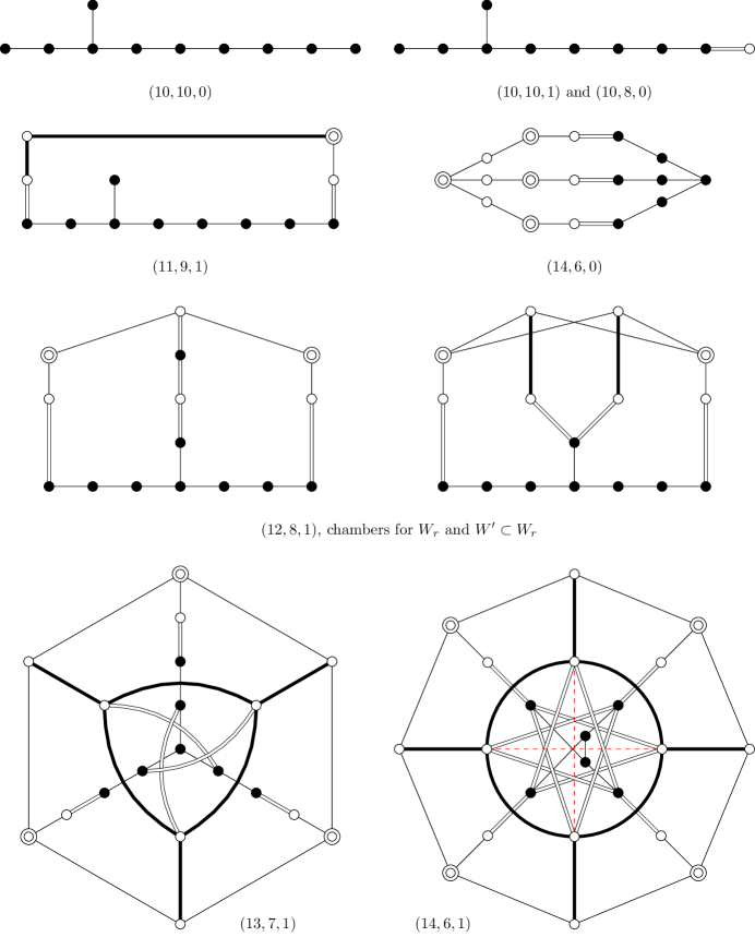
Figure 3. Coxeter diagrams for lattices on the $g=1$ line, part 1

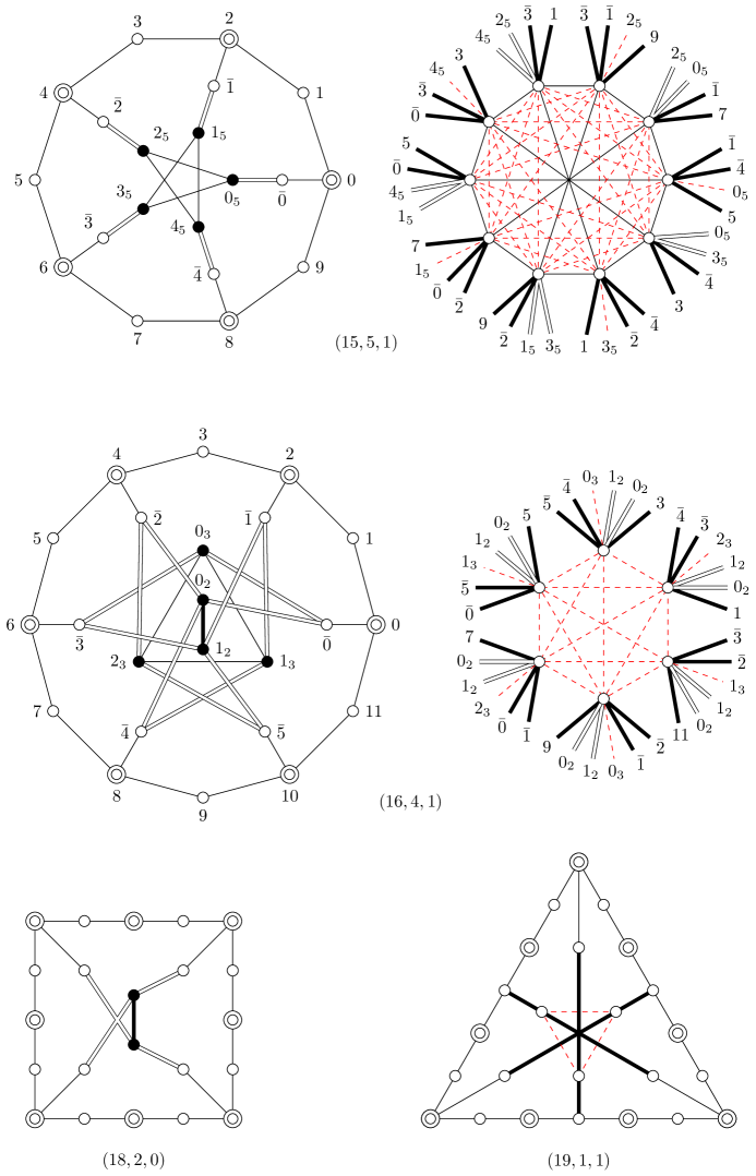
Figure 4. Coxeter diagrams for lattices on the $g=1$ line, part 2

Remark 3.7.

The $(12,8,1)$ diagram contains the subdiagram ${\widetilde{B}}_{3}$ which generates the same lattice as ${\widetilde{A}}_{3}$. As in Lemma 3.3, let ${\mathbb{B}}$ consist of the isolated $(-4)$-vector, so that $W({\mathbb{B}})=S_{2}$. Reflecting the attached $(-2)$-vectors gives two other $(-2)$-vectors. One of them forms the ${\widetilde{A}}_{3}$ diagram with the others. This gives the Coxeter diagram for an index 2 reflection subgroup $W^{\prime}\subset W_{\rm r}$, also shown in Fig. 3. The righthand diagram is of greater relevance for later constructions.

The diagrams for $(15,5,1)$ and $(16,4,1)$ are quite large so drawn in two parts.

Remark 3.8.

The overarching reason for the two exceptional cases is that the lattices on the $g=1$ line are mirrors of the double covers of del Pezzo surfaces. The del Pezzo surfaces of Picard rank $n+1$ correspond to the $E_{n}$ lattices. For $n\geq 3$ they are root lattices: $A_{2}A_{1}$, $A_{4}$, $D_{5}$, $E_{6}$, $E_{7}$, $E_{8}$. But the $E_{2}$ lattice of degree $7$ is not a root lattice, its root sublattice has corank $1$. And for $n=1$ there are two types $E_{1}$, $E_{1}^{\prime}$ corresponding to ${\mathbb{F}}_{1}$ and ${\mathbb{F}}_{0}$. The lattice $E_{1}^{\prime}$ corresponding to ${\mathbb{F}}_{0}$ has a finite index root sublattice $A_{1}$. But the lattice $E_{1}$ corresponding to ${\mathbb{F}}_{1}$ has an empty root lattice. See more about these in [ABE22].

3E. Coxeter diagrams for $(18,2,1)$ and $(17,3,1)$

Here we treat the two exceptional cases which do not have finite covolume. The following is the result of applying Vinberg’s algorithm.

$(18,2,1)$. There are no $(-4)$-vectors of divisibility $2$ in this lattice $S$, and since the automorphism group of a K3 surface with this Picard lattice is infinite, there are infinitely many $(-2)$-vectors, so the Coxeter diagram is infinite. Rather than attempting to draw it, we describe it in words.

There is a wheel ${\widetilde{A}}_{15}$ of $16$ $(-2)$-curves forming a singular fiber of an elliptic fibration. In addition to them there are $8$ sections $a_{0},a_{2},\dotsc,a_{14}$ attached to $e_{0},e_{2},\dotsc a_{14}$ singly, i.e. with $(a_{i},e_{j})=\delta_{ij}$; and bisections $b_{1},b_{3},\dotsc,b_{15}$ with $(b_{i},e_{j})=2\delta_{ij}$. The bisections have divisibility $2$.

Let ${\widetilde{A}}_{15}^{\perp}=\langle c,v\rangle$ with $c$ the class of the fiber. The Eichler transformation $E=E_{c,v}$ [Sca87, 3.7] is an isometry $S$ which fixes the vertices of ${\widetilde{A}}_{15}$. The orbits $a_{i}^{n}:=E^{n}(a_{i})$ and $b_{i}^{n}:=E^{n}(b_{i})$ are the remaining $(-2)$-vectors. Each orbit is isomorphic to ${\mathbb{Z}}$.

For the typical representatives $a_{0}=a_{0}^{0}$ and $b_{1}=b_{1}^{0}$ we list the vectors with intersections $0,2$. All the other $a_{i}^{n}$ and $b_{i}^{n}$ have intersections $>2$ and give dashed edges in the Coxeter diagram.

For $a_{0}$ the $(-2)$-vectors outside of the ${\widetilde{A}}_{15}$ cycle with intersections $0,2$ are:

1. $a_{2}^{0}$, $a_{4}^{1}$, $a_{6}^{1}$, $a_{10}^{2}$, $a_{12}^{2}$, $a_{14}^{3}$ and $b_{1}^{0}$, $b_{3}^{0}$, $b_{13}^{2}$, $b_{15}^{2}$.

2. $a_{2}^{1}$, $a_{8}^{1}$, $a_{8}^{2}$, $a_{14}^{2}$ and $b_{7}^{1}$, $b_{9}^{1}$.

For $b_{1}$ the $(-2)$-vectors outside of the ${\widetilde{A}}_{15}$ cycle with intersections $0,2$ are:

1. $a_{0}^{0}$, $a_{2}^{1}$, $a_{4}^{1}$, $a_{14}^{3}$.

2. $a_{8}^{2}$, $a_{10}^{2}$.

The other intersection numbers are recovered by the fact that $E$ is an isometry, the cyclic symmetry $(u_{i},v_{j})=(u_{i-k},v_{j-k})$ ($u,v\in\{a,b\}$) for as long as all the indices stay in $\{0,\dotsc 15\}$. Going around the circle the shift is $u_{i+16}^{n}=u_{i}^{n-3}$. For example,

$$(b_{15},a_{6}^{-1})=(b_{9},a_{0}^{-1})=(b_{9}^{1},a_{0}^{0})=2,$$

$$(a_{14}^{3},a_{2}^{1})=(a_{12}^{3},a_{0}^{1})=(a_{12}^{2},a_{0}^{0})=0,$$

$$(b_{15},a_{16}^{1})=(b_{15},a_{0}^{-2})=(b_{15}^{2},a_{0}^{0})=0.$$

Example 3.9.

$b_{1}$ is a $(-2)$-vector of divisibility $2$ which does not lie on the ${\widetilde{A}}_{15}$-cycle. The vectors which have intersection $0$ with $b_{1}$ are $e_{i}$ for $i\neq 1$ and $a_{14}^{3}$, $a_{0}^{0}$, $a_{2}^{1}$, $a_{4}^{1}$. The last four vectors are mutually orthogonal with the exception of $(a_{0}^{0},a_{2}^{1})=2$. We conclude that these $15+4$ vectors form the Coxeter diagram for the lattice $(17,1,1)$ that was given in [AN06, Table 1]. This agrees with Lemma 4.15.

$(17,3,1)$. Both the diagrams for the full reflection group $W_{\rm r}$ and the reflection group $W_{2}$ in $(-2)$-vectors are infinite. We compute the latter one.

There is a wheel ${\widetilde{A}}_{13}$ of $14$ $(-2)$-curves forming a singular fiber of an elliptic fibration. In addition to them there are $7$ sections $a_{0},a_{2},\dotsc,a_{12}$ attached to $e_{0},e_{2},\dotsc a_{12}$ singly, i.e. with $(a_{i},e_{j})=\delta_{ij}$; and bisections $b_{1},b_{3},\dotsc,b_{13}$ with $(b_{i},e_{j})=2\delta_{ij}$. The bisections have divisibility $2$.

Let ${\widetilde{A}}_{13}^{\perp}=\langle c,v_{1},v_{2}\rangle$ with $c$ the class of the fiber. For $v\in{\widetilde{A}}_{13}^{\perp}$ the Eichler transformation $E=E_{c,v}$ is an isometry $S$ which fixes the vertices of ${\widetilde{A}}_{15}$. We pick $v_{1},v_{2}$ so that their intersection form is $\begin{pmatrix}-4&2\\ 2&-8\end{pmatrix}.$ The orbits

$$a_{i}^{n_{1},n_{2}}:=E_{c,n_{1}v_{1}+n_{2}v_{2}}(a_{i}),\quad b_{i}^{n_{1},n_{2}}:=E_{c,n_{1}v_{1}+n_{2}v_{2}}(b_{i})$$

are the remaining $(-2)$-vectors. Each orbit is isomorphic to ${\mathbb{Z}}^{2}$. Note that $E_{c,n_{1}v_{1}}$ is contained in the Weyl group $W({\widetilde{A}}_{1})$ generated by the reflections in the $(-4)$-vectors $v_{1}$ and $c-v_{1}$.

For the typical representatives $a_{0}=a_{0}^{0,0}$ and $b_{1}=b_{1}^{0,0}$ we list the vectors with intersections $0,2$. All the other $a_{i}^{n_{1},n_{2}}$ and $b_{i}^{n_{1},n_{2}}$ have intersections $>2$ and give dashed edges in the Coxeter diagram.

For $a_{0}$ the $(-2)$-vectors outside of the ${\widetilde{A}}_{13}$ cycle with intersections $0,2$ are:

1. $a_{0}^{-1,0}$, $a_{0}^{1,0}$,  $a_{2}^{0,0}$, $a_{2}^{0,1}$, $a_{2}^{1,1}$,  $a_{4}^{0,1}$, $a_{4}^{1,1}$,  $a_{6}^{1,2}$,  $a_{8}^{1,2}$,  $a_{10}^{1,3}$, $a_{10}^{2,3}$,
   $a_{12}^{1,3}$, $a_{12}^{2,3}$, $a_{12}^{2,4}$;   $b_{1}^{0,0}$, $b_{1}^{1,0}$,  $b_{3}^{1,1}$,  $b_{11}^{2,3}$,  $b_{13}^{2,4}$, $b_{13}^{3,4}$.

2. $a_{0}^{-1,-1}$, $a_{0}^{0,-1}$, $a_{0}^{0,1}$, $a_{0}^{1,1}$,  $a_{2}^{-1,0}$, $a_{2}^{1,0}$,  $a_{4}^{1,2}$,  $a_{6}^{0,1}$, $a_{6}^{0,2}$, $a_{6}^{1,1}$, $a_{6}^{2,2}$,
   $a_{8}^{0,2}$, $a_{8}^{1,3}$, $a_{8}^{2,2}$, $a_{8}^{2,3}$,  $a_{10}^{1,2}$,  $a_{12}^{1,4}$, $a_{12}^{3,4}$;   $b_{1}^{1,1}$,  $b_{5}^{1,1}$,  $b_{7}^{1,2}$, $b_{7}^{2,2}$,  $b_{9}^{2,3}$,  $b_{13}^{2,3}$.

For $b_{1}$ the $(-2)$-vectors outside of the ${\widetilde{A}}_{13}$ cycle with intersections $0,2$ are:

1. $a_{0}^{-1,0}$, $a_{0}^{0,0}$,  $a_{2}^{-1,0}$, $a_{2}^{0,0}$,  $a_{4}^{0,1}$,  $a_{12}^{1,3}$.

2. $a_{0}^{-1,-1}$,  $a_{2}^{0,1}$,  $a_{6}^{0,1}$,  $a_{8}^{0,2}$, $a_{8}^{1,2}$,  $a_{10}^{1,3}$.

The other intersection numbers are recovered by the fact that Eichler transformations are isometries, the symmetries $(u_{i},v_{j})=(u_{i-k},v_{j-k})$ ($u,v\in\{a,b\}$) for as long as all the indices stay in $\{0,\dotsc 13\}$. Going around the circle the shift is $u_{i+14}^{n_{1},n_{2}}=u_{i}^{n_{1}-2,n_{2}-4}$.

Example 3.10.

$b_{1}$ is a $(-2)$-vector of divisibility $2$ which does not lie on the ${\widetilde{A}}_{13}$-cycle. The vectors which have intersection $0$ with $b_{1}$ are $e_{i}$ for $i\neq 1$ and $a_{0}^{-1,0}$, $a_{0}^{0,0}$, $a_{2}^{-1,0}$, $a_{2}^{0,0}$, $a_{4}^{0,1}$, $a_{12}^{1,3}$. Using the rules above, we obtain that $(a_{0}^{0,0},a_{2}^{-1,0})=(a_{0}^{-1,0},a_{2}^{0,0})=2$ and all the other intersection numbers among these six vectors are zero. This is the same diagram of $(-2)$-curves as the one for the $(16,2,1)$ lattice obtained from the Coxeter diagram given in [AN06, Table 1] by applying the Weyl group $W(A_{1})=S_{2}$ for the unique black vertex. This agrees with Lemma 4.15.

3F. Lattices on the $g=0$ line

Several of the lattices on the $g=0$ line have finite Coxeter diagrams. They are quite large and complicated. We don’t need them for the present paper since they don’t appear as targets of the mirror moves 5.6, see Remark 5.7. So we don’t include them here; they will appear elsewhere.

4. K3 surfaces, their quotients, and the nef cones

We give a brief description for the K3 surfaces $X$ and their quotients $Y$ that appear in the $75$ families of Fig. 1.

4A. Surfaces for $S$ with $g\geq 2$, excluding $(10,8,0)$

For the $50$ lattices with $g\geq 2$, excluding $(10,8,0)$, a satisfactory description for the quotients $Y$ is given in [AN06]. Indeed, all the possibilities for the exceptional curves on the surfaces $Y$ appearing in these families were found. From the graph of exceptional curves one can realize $Y$ as an explicit blowup of ${\mathbb{P}}^{2}$ or ${\mathbb{F}}_{n}$. The K3 surfaces $X$ are double covers of $Y$ branched in some divisor $B$ lying in the linear system $|-2K_{Y}|$.

For the most basic lattices $(r,r,\delta)$ with $r\leq 9$, the surfaces $Y$ are weak del Pezzo surfaces with big and nef $-K_{Y}$ and with $ADE$ singularities. Thus, $Y=\operatorname{Bl}_{r-1}{\mathbb{P}}^{2}$ for $(r,r,1)$ and $Y={\mathbb{P}}^{1}\times{\mathbb{P}}^{1}$ or ${\mathbb{F}}_{2}$ for $(2,2,0)$.

4B. Surfaces for $S$ on the $g=1$ line and $(10,8,0)$

This case is especially important for us since it serves as the base case for the mirror symmetry constructions and all the other cases are derived from it.

Theorem 4.1 (Nikulin).

Let $X$ be a K3 surface with a nonsymplectic involution $\iota$ and $2$-elementary Picard lattice $S=\operatorname{Pic}X$. Denote $\pi\colon X\to Y=X/\iota$. Then the automorphism group $\operatorname{Aut}X$ is infinite and preserves a (necessarily unique) elliptic pencil $f\colon X\to{\mathbb{P}}^{1}$ if and only if $S$ is one of the following lattices:

1. $I_{2k}I_{0}$: $(10+k,10-k,\delta)\neq(14,6,0)$ and $k>0$. $Y$ is a rational elliptic surface with a section and the ramification divisor

   $$R=X^{\iota}=F_{0}\cup\cup_{i=0}^{k-1}E_{2i},$$

   where $F_{0}$ is a smooth elliptic fiber, and $E_{i}$ are disjoint ${\mathbb{P}}^{1}$s which are the alternating curves in the $I_{2k}$ fiber $F$ of Kodaira type $I_{2k}$ (a wheel of $2k$ rational curves).

2. $I_{0}^{2}$: $(10,8,0)$. $R=F_{0}\cup F$ is a union of two smooth fibers of $f$.

3. Halphen: $(10,10,1)$. $Y$ is an index $2$ Halphen pencil and $R=F_{0}$ is a smooth elliptic fiber which does not ramify over the unique multiple fiber $G=2D$ on $Y$.

4. Enriques: $(10,10,0)$. $Y$ is an Enriques surface and $R=\emptyset$.

5. ${\widetilde{E}}_{6}$: $(14,6,0)$: $R$ is the sum of a smooth elliptic fiber $F_{0}$ and $4$ disjoint ${\mathbb{P}}^{1}$s, alternating curves in a $IV^{*}$ fiber.

In the $I_{0}^{2}$ case one has $g=2$, in the other cases one has $g=1$.

Proof.

[Nik81, Sec. 4] and [Nik20]. ∎

We will call (1,2,3) the ordinary cases. The case (5) does not appear on the mirror side in our constructions.

4C. Surfaces for $S$ on the $g=0$ line

The lattices $(10+k,12-k,\delta)$ for $1\leq k\leq 9$ are in a bijection with the lattices $(10+k,10-k,\delta)$ on the line below in Fig. 1, excluding $(14,6,0)$, which is the (${\widetilde{E}}_{6}$) case of Theorem 4.1.

Consider one of the lattices $S^{\prime}=(10+k,10-k,\delta)$, $1\leq k\leq 9$ on the $g=1$ line. This is the case (1) of Theorem 4.1. The quotient $Y^{\prime}$ is a rational elliptic surface with a section and $\pi\colon X^{\prime}\to Y^{\prime}$ is ramified in a smooth elliptic fiber $F_{0}$ and ramified in the $n$ alternating curves $(-4)$-curves $E_{2i}$. It follows that $S^{\prime}=U\oplus K$ for some negative definite lattice $K$. (Indeed, these are the lattices $A_{2k-1}E_{9-k}(2)$ of Table 2.)

Now let $S=U(2)\oplus K$. Then $S=(10+k,12-k,\delta)$ is the corresponding lattice on the $g=0$ line. The line bundle corresponding to an isotropic vector in $U(2)$ defines an elliptic fibration $f\colon X\to{\mathbb{P}}^{1}$ without a section whose jacobian fibration is $f^{\prime}\colon X^{\prime}\to{\mathbb{P}}^{1}$. The fiber corresponding to $F$ is a double fiber of $f$ and the ramification divisor of $\pi\colon X\to Y$ is the union of the $n$ curves $E_{2i}$. The surface $X$ can be obtained from $X^{\prime}$ directly by a logarithmic transformation at $F$ using [CD89, Cor. 5.4.7].

So these K3 surfaces $X$ are the index 2 Halphen K3 surfaces with an $I_{2k}$ fiber. The surfaces ${\overline{Y}}$ obtained by contracting the $(-1)$-curves in the special fiber are the rational index $2$ Halphen pencils with an $I_{k}$ fiber. Some explicit constructions for such pencils were given in [Kim18, Kim20, Zan20].

Finally, the moduli space for the lattice $(20,2,1)$ is a point. It is the unique “most algebraic” $2$-elementary K3 surface of [Vin83]. It admits no Halphen pencils but we computed that up to automorphisms, it has $13$ elliptic pencils with a section.

4D. Nef cones and exceptional curves on $X$ and $Y$

It is well known that the nef cone of a K3 surface $X$ is defined by linear inequalities in the positive cone $\overline{{\mathcal{C}}}=\{v\in S_{X}\otimes{\mathbb{R}}\mid x^{2}\geq 0,\ x\cdot h\geq 0\}$, where $h$ is a Kähler class, with facets $x\cdot E_{i}\geq 0$ for the smooth rational curves $E_{i}$ with $E_{i}^{2}=-2$, which we call the $(-2)$-curves. Their classes in $\operatorname{NS}(X)$ are the positive roots for the Weyl group $W_{2}(S_{X})$. For any $(-2)$-vector $v\in\operatorname{NS}(X)$, exactly one of $\pm v$ is effective and is a sum of $(-2)$-curves.

Since a $(-2)$-curve is uniquely determined by its class in $\operatorname{NS}(X)$, any involution preserving its class preserves the $(-2)$-curve, but may not fix it pointwise.

We call a curve exceptional if it is irreducible and has negative self-intersection. $R=X^{\iota}$ will denote the ramification divisor of $\pi\colon X\to Y$ and $B\subset Y$ the branch divisor.

Lemma 4.2.

Exceptional curves $F$ on $Y$ are of three types:

1. $F^{2}=-4$, $\pi^{*}(F)=2E$, and the $(-2)$-curve $E\subset X^{\iota}$ is fixed pointwise by the involution.

2. $F^{2}=-1$, $\pi^{*}(F)=E$, $|F\cap B|=|E\cap R|=2$.

3. $F^{2}=-1$, $\pi^{*}(F)=E_{1}+E_{2}$, $F$ is tangent to $B$, the curves $E_{1}$, $E_{2}$ are exchanged by the involution and $E_{1}\cdot E_{2}=1$.

4. $F^{2}=-2$, $\pi^{*}(F)=E_{1}+E_{2}$, $F\cap B=E_{i}\cap R=\emptyset$, the curves $E_{1}$, $E_{2}$ are disjoint and are exchanged by the involution.

Proof.

[AN06, Sec. 2.4]. ∎

Lemma 4.3.

$\operatorname{Nef}Y=(\operatorname{Nef}X)\cap S_{\mathbb{R}}$, where $S=S_{X}^{+}$

Proof.

This follows from the identities $\iota^{*}\circ\iota_{*}=1+\iota$ and $\iota_{*}\circ\iota^{*}=2$. ∎

Definition 4.4.

Let $\operatorname{Cur}_{2}=\{F_{i}\}$ be the set of the $(-2)$-curves on $Y$, i.e. of type (3) in Lemma 4.2. Let $\pi^{*}(F)=E_{1}+E_{2}$ be the corresponding $(-4)$-vectors in $S$. It is obvious that for any $v\in S$ one has $\pi^{*}(F)\cdot v=2E_{1}\cdot v\in 2{\mathbb{Z}}$. They are also primitive since $(\pi^{*}(F)/2)^{2}=-1$ and $S$ is an even lattice. So they are simple roots for the full reflection group $W_{\rm r}(S)$ and they correspond to a subset ${\mathbb{B}}$ of black vertices in the Coxeter diagram of $S$ as in Definition 3.2.

Lemma 4.5.

$\operatorname{Nef}Y=W({\mathbb{B}}).{\mathfrak{C}}_{\rm r}$, where ${\mathfrak{C}}_{\rm r}$ is a fundamental chamber for $W_{\rm r}(S)$. The set of exceptional curves on $Y$ is identified with the union of $W({\mathbb{B}})$-orbits of white vertices in the Coxeter diagram of $S$.

Proof.

This follows by Corollary 3.4 and the description of $\operatorname{Nef}X$ above. ∎

4E. Surfaces $Y$ with the smallest nef cone

Proposition 4.6.

For each lattice $S\neq(10,10,0)$, with $g\geq 1$ of Fig. 1 there exists a K3 surface with $S_{X}^{+}=S$ such that $\operatorname{Nef}Y$ can be identified with the Coxeter chamber for the full reflection group $W_{\rm r}$ if $S\neq(12,8,1)$, and the Coxeter chamber for an index $2$ subgroup $W^{\prime}\subset W_{\rm r}$ if $S=(12,8,1)$.

Proof.

In view of Lemma 4.5 we need to find a quotient surface $Y$ on which the $(-2)$-curves form the entire black subdiagram of the Coxeter diagram, for $S\neq(12,8,1)$.

In the $(12,8,1)$ case we consider the fundamental chamber ${\mathfrak{C}}^{\prime}_{\rm r}$ for the index $2$ subgroup of $W^{\prime}\subset W_{\rm r}$, a union of two fundamental chambers ${\mathfrak{C}}_{\rm r}$ and $w{\mathfrak{C}}_{\rm r}$ where $w$ is the reflection in the isolated $(-4)$-root. This modified chamber is also pictured in Fig. 3. The corresponding surface has an $I_{2}$ fiber.

For the $50$ lattices with $g\geq 2$ and different from $(10,8,0)$ existence of such $Y$ is a small part of [AN06] where all possibilities for the sets of exceptional curves were classified. The surfaces we need here are “the most degenerate”, they all appear in [AN06, Table 3].

For the surfaces with an elliptic pencil with a section we take for $Y$ one of the surfaces of Table 1. They exist by [Per90]; see also [MP86, OS91].

Case	Singular fibers	Fiber root lattice	$MW(Y)$
$(10,10,1)$	${}_{2}I_{0}II^{*}+I_{1}^{2}$	$E_{8}$	$\emptyset$
$(10,8,0)$	$II^{*}+I_{1}^{2}$	$E_{8}$	$0$
$(11,9,1)\ A_{0}E_{8}$	$I_{1}II^{*}+I_{1}$	$E_{8}$	${\mathbb{Z}}_{1}$
$(12,8,1)\ A_{1}E_{7}$	$I_{2}\,III^{*}+I_{1}$	$A_{1}E_{7}$	${\mathbb{Z}}_{2}$
$(13,7,1)\ A_{2}E_{6}$	$I_{3}IV^{*}+I_{1}$	$A_{2}E_{6}$	${\mathbb{Z}}_{3}$
$(14,6,1)\ A_{3}E_{5}$	$I_{4}I_{1}^{*}+I_{1}$	$A_{3}D_{5}$	${\mathbb{Z}}_{4}$
$(15,5,1)\ A_{4}E_{4}$	$I_{5}I_{5}+I_{1}^{2}$	$A_{4}A_{4}$	${\mathbb{Z}}_{5}$
$(16,4,1)\ A_{5}E_{3}$	$I_{6}I_{3}I_{2}+I_{1}$	$A_{5}A_{2}A_{1}$	${\mathbb{Z}}_{6}$
$(17,3,1)\ A_{6}E_{2}$	$I_{7}I_{2}+I_{1}II$	$A_{6}A_{1}$	${\mathbb{Z}}$
$(18,2,1)\ A_{7}E_{1}$	$I_{8}+I_{1}^{2}II$	$A_{7}$	${\mathbb{Z}}$
$(18,2,0)\ A_{7}E^{\prime}_{1}$	$I_{8}I_{2}+I_{1}^{2}$	$A_{7}A_{1}$	${\mathbb{Z}}_{2}^{2}$
$(19,1,1)\ A_{8}E_{0}$	$I_{9}+I_{1}^{3}$	$A_{8}$	${\mathbb{Z}}_{3}$

Table 1. Special rational elliptic surfaces $Y$

In the $(10,10,1)$ Halphen case, the surface with a double ${}_{2}I_{0}$ fiber can be obtained from a $(10,8,0)$ surface by a logarithmic transformation along a smooth $I_{0}$ fiber using [CD89, Cor. 5.4.7]. ∎

Remark 4.7.

Most of the surfaces of Table 1 are the maximally degenerate ones in their families but some are not: For $(12,8,1)$ the most degenerate surface has $III^{*}III$ fibers, and for $(10,10,1)$ the ${}_{2}I_{1}II^{*}I_{1}$ fibers.

We use a logical notation $A_{k-1}E_{9-k}$ to denote the cases $(10+k,10-k,\delta)$ for $1\leq k\leq 9$. Here, $E_{k}$ is the lattice $K^{\perp}$ in the Picard lattice for a a del Pezzo surface of degree $K^{2}=9-k$. For $k=1$ there are two cases, $E_{1}$ for ${\mathbb{F}}_{1}$ and $E^{\prime}_{1}$ for ${\mathbb{F}}_{0}$.

Corollary 4.8.

For the surfaces $Y$ of Proposition 4.6, the Coxeter diagram of $S$ also serves as the dual graph of exceptional curves, with the following modifications:

1. Vertices: the double circled white, single white circles, and black vertices respectively correspond to ${\mathbb{P}}^{1}$ with $F^{2}=-4$, $-1$, $-2$ respectively.

2. Edges: $F_{i}\cdot F_{j}=1$ for a white vertex $F_{i}$ and a black vertex $F_{j}$ or for two single circled white vertices. The other intersection numbers are: $F_{i}\cdot F_{j}=1$ for a single edge, and $2$ for a bold edge in the diagram.

4F. The Heegner divisor hierarchy

Definition 4.9 (Heegner moves).

The $(-1,-1)$-move goes from a node $(r,a,1)$ of Fig. 1 to the node $(r-1,a-1,\delta)$. We call it ordinary if $\delta=1$ and characteristic if $\delta=0$. The opposite $(+1,+1)$-move goes from $(r,a,\delta)$ to $(r+1,a+1,1)$. The $(+1,-1)$-move is from $(r,a)$ to $(r+1,a-1)$ and the opposite $(-1,+1)$-move is from $(r,a)$ to $(r-1,a+1)$.

For the rest of this section, we exclude the lattice $S=(10,8,0)$ which is in many ways exceptional, cf. Remark 2.1.

Lemma 4.10.

Let $S=(r,a,\delta)$ and ${\mathbb{D}}_{S}$ be its period domain, $S\rightarrowtail S^{\prime}=(r^{\prime},a^{\prime},\delta^{\prime})$ be a $(+1,+1)$ or $(+1,-1)$-move. Then $S^{\prime}$ defines a Heegner divisor ${\mathbb{D}}_{S^{\prime}}\subset{\mathbb{D}}_{S}$ on which the K3 surfaces acquire an additional $(-2)$-curve $E$, preserved by the involution on K3 surfaces over $S^{\prime}$. For the $(+1,+1)$-move, this involution preserves but does not fix $E$ and for the $(+1,-1)$-move, it fixes $E$ pointwise.

Proof.

Let $X\to(C,0)$ be a smooth family of K3 surfaces with $[X_{0}]$ generic in ${\mathbb{D}}_{S^{\prime}}$, i.e. $H^{2}(X_{0},{\mathbb{Z}})^{+}=S^{\prime}$ and with $[X_{t}]\in{\mathbb{D}}_{S}\setminus{\mathbb{D}}_{S^{\prime}}$ for $t\neq 0$. Let $R_{t}$ be the ramification divisor on $X_{t}$, $t\neq 0$, ${\overline{R}}_{0}$ be its flat limit, and $R_{0}$ be the ramification divisor of the involution of $X_{0}$ determined by $S^{\prime}$. Then for a

1. $(+1,+1)$-move: $k_{0}=k$, $g_{0}=g-1$, and ${\overline{R}}_{0}=R_{0}\cup E$.

2. $(+1,-1)$-move: $g_{0}=g$, $k_{0}=k+1$ and $R_{0}={\overline{R}}_{0}\sqcup E$.

This is proven by considering the small contraction $X\to{\overline{X}}$ which contracts $E$ to a point. The birational involution on $X$ equaling $\iota_{t}$ on the general fiber extends to a regular involution of ${\overline{X}}$ and the two cases are distinguished simply by whether the contraction of $E$ lies on the limit of $R_{t}$ (necessarily a node of the limiting curve) or is disjoint from the limit. In the former $(+1,+1)$ case, the involution on the minimal resolution $X_{0}\to{\overline{X}}_{0}$ preserves $E$ but only fixes the two branches of the node. In the latter $(+1,-1)$ case, the involution on $X_{0}$ fixes $E$ pointwise, because the contraction of $E$ is isolated in the fixed locus of the involution on ${\overline{X}}_{0}$. ∎

Lemma 4.11.

Any $2$-elementary lattice with $g\geq 1$ has the form

$$S=\big{(}10+k-(g-1),10-k-(g-1),\delta\big{)}$$

and it can be reached from one of the lattices of Section 4B with $g=1$ by $g-1$ total $(-1,-1)$-moves.

Proof.

One look at Fig. 1 confirms this. ∎

Next, we want to understand how Coxeter diagrams change.

Lemma 4.12.

For the lattices related by a $(-1,-1)$-move one has $S=S^{\prime}\oplus A_{1}$ and a generator $r$ of $A_{1}$ is a $(-2)$-root of divisibility $2$. For any hyperbolic lattice $S=(r,a,1)$ there exists exactly one or two $O(S)$-orbits of $(-2)$-roots of divisibility $2$, and these vectors are in a bijection with the $(-1,-1)$-moves down from $S$.

In terms of the Coxeter diagram $\Gamma$, for any $S\neq(10,8,0)$ they are in bijection with the $\operatorname{Aut}\Gamma$-orbits of white vertices in $\Gamma$ which are not connected to some neighbor by a single (i.e. weight $1$) edge.

Proof.

One has

$$S^{\prime}\oplus A_{1}=(r-1,a-1,\delta)_{1}+(1,1,1)_{0}=(r,a,1)_{1}\simeq S.$$

For $S=S^{\prime}\oplus A_{1}=S^{\prime\prime}\oplus A_{1}$ with $S^{\prime},S^{\prime\prime}$ of the same type, an isometry $S^{\prime}\to S^{\prime\prime}$ defines an isometry $S\to S$, so there is exactly one $O(S)$-orbit. The generator of $A_{1}$ is a $(-2)$-root and it clearly has divisibility $2$. By Prop. on p.2 of [Vin83] such roots lie in different $W_{\rm r}$-orbits. One has $O(S)=\operatorname{Aut}\Gamma\ltimes W_{\rm r}$, so two such roots in the same orbit must differ by a diagram symmetry. Finally, for all the lattices in Fig. 1 with the exception of $(10,8,0)$ the roots generate the lattice, so $\operatorname{div}(r)=2$ iff $r\cdot r_{i}$ is even for the other roots, which is read off directly from the diagram. ∎

Corollary 4.13.

Any lattice in Fig. 1 with $g\geq 1$ is of the form

$$S=\big{(}10+k-(g-1),10-k-(g-1),\delta\big{)}.$$

It can be reached from the “base” lattice $S_{1}=(10+k,10-k,1)=S\oplus A_{1}^{g-1}$ by a sequence of $(-1,-1)$-moves which corresponding to a chain of vertices $\alpha_{1},\dotsc,\alpha_{g-1}$ with colors white-black-…-black, in the Coxeter diagram $\Gamma_{\rm r}(S)$, with $\alpha_{1}$ an even $(-2)$-root. This chain is unique up to $\operatorname{Aut}\Gamma$.

Remark 4.14.

The $(+1,-1)$ moves play a particularly important role from the perspective of moduli, because of Lemma 4.10. Recall that $F_{S}=({\mathbb{D}}_{S}\setminus\Delta)/O(T)$. The divisors in $\Delta/O(T)$ correspond to Heegner divisor moves of either $(+1,-1)$ type or $(+1,+1)$-type. For a Heegner divisor of $(+1,-1)$-type, the involution on the limiting of K3 surface has an extra $(-2)$-curve, fixed pointwise by the involution, but the flat limit of a positive genus fixed component $C_{g}$ equals the positive genus fixed component. Thus from the perspective of the KSBA compactification $F_{S}\hookrightarrow{\overline{F}}_{S}$ for pairs $({\overline{X}},\epsilon{\overline{C}}_{g})$, the $(+1,-1)$-move plays essentially no role, except to restrict to a Noether-Lefschetz subdomain of ${\overline{F}}_{S}$.

Thus, it suffices to compactify the moduli space $F_{S}$ for lattices $S$ on the $k=0$ line, and the other cases follow by induction. For the hyperbolic $2$-elementary lattices ${\overline{T}}=I^{\perp}/I$ associated to Type III cusps of $F_{S}$ (cf. Sec. 5), the action of a $(+1,-1)$ Heegner move on $S$ is a $(-1,-1)$ move on ${\overline{T}}$. This is why Corollary 4.13 is relevant: We can reach all necessary hyperbolic lattices for semitoroidal compactifications from those on the $g=1$ line.

Lemma 4.15.

The Coxeter diagram $\Gamma^{\prime}$ of $S^{\prime}$ is obtained from the diagram $\Gamma$ of $S=S^{\prime}\oplus A_{1}$ by removing the vertex $r$, removing the adjacent white vertices, turning black adjacent vertices to white and, if there exist $(-4)$-roots $\alpha_{1},\alpha_{2}$ with $\alpha\cdot\alpha_{1}=\alpha\cdot\alpha_{2}=2$, connecting their images in $\Gamma_{1}$ by a double line.

Proof.

The fundamental chamber for $S^{\prime}$ is the face $\alpha^{\perp}$ of the fundamental chamber for $S^{\prime}\oplus A_{1}$. The facets of this chamber are of the form $p(\alpha_{i})^{\perp}$ where $p(\alpha_{i})$ are the orthogonal projections of the roots defining the facets for $S$ for which $p(\alpha_{i})^{2}<0$. The formula $p(\alpha_{1})\cdot p(\alpha_{2})=\alpha_{1}\cdot\alpha_{2}+\frac{1}{2}(\alpha\cdot\alpha_{1})(\alpha\cdot\alpha_{2})$ implies the rest: For the $(-2)$-neighbors $\alpha_{1}$ of $\alpha$ with $\alpha\cdot\alpha_{1}=2$ one gets $p(\alpha_{1})^{2}=0$, so they are not faces of $\alpha^{\perp}$, and for $(-4)$-neighbors with $\alpha\cdot\alpha_{1}=2$ one gets $p(\alpha_{1})^{2}=-2$, so they change their color. ∎

Lemma 4.16.

Let $S,S_{1}$ and $\alpha_{1},\dotsc,\alpha_{g-1}$ be as in Corollary 4.13. Let $G\subset\Gamma(S)$ and $G_{1}\subset\Gamma(S_{1})$ be the subdiagrams such that for the vertices one has $V(S_{1})=V(S)\cup\{\alpha_{1},\dotsc,\alpha_{g}\}$. Then

1. $G_{1}$ is elliptic iff $G$ is too, and no vertex of $G$ is a neighbor of $\alpha_{1},\dotsc,\alpha_{g-1}$.

2. $G_{1}$ is maximal parabolic if $G$ contains a parabolic subdiagram and either no vertex of $G$ is a neighbor of $\alpha_{1},\dotsc,\alpha_{g-1}$ or $g-1=1$ and $\alpha_{1}$ neighbors one isolated vertex of $G$.

Proof.

If $\beta$ is a vertex of $G$ attached to $\alpha_{1}$ then $\beta^{2}=-2$ and $\beta\cdot\alpha_{1}=2$, so $\langle\beta,\alpha_{1}\rangle={\widetilde{A}}_{1}$ is already parabolic. (1) immediately follows. In the parabolic case, maximal parabolic subgraphs have rank $\operatorname{rk}S-1$, so the remaining part is nonempty and contains a nonempty maximal parabolic subdiagram. For the exceptional cases $S_{1}=(18,2,1)$ and $(17,3,1)$ the diagrams for the lattice $S_{2}=(17,1,1)$, resp. $(16,2,1)$ contain parabolic subdiagrams ${\widetilde{D}}_{14}$, resp. ${\widetilde{D}}_{12}$ disjoint from ${\widetilde{A}}_{1}$. ∎

Lemma 4.17.

For the surfaces of Corollary 4.8 for which the Coxeter diagram is the dual graph of the exceptional curves on the quotients, the surface $Y_{1}$ is obtained from $Y$ by contracting a $(-1)$-curve $F$ not contained in the branch divisor $B$. The surface $X_{1}$ is obtained from $X$ by contracting a $(-2)$-curve not contained in the ramification divisor $R$, and then smoothing the singular K3 surface together with an involution.

Remark 4.18.

The $(+1,-1)$ and $(-1,+1)$ moves in Fig. 1 do not admit such an easy description. In those cases $S$ corresponds to an index $2$ overlattice of $S^{\prime}\oplus A_{1}$. The $(r,a,\delta_{1})\rightarrowtail(r-1,a+1,\delta)$ move can be understood as contracting a $(-4)$-curve on $Y^{\prime}$ and then smoothing. For example, $(2,0,0)\rightarrowtail(1,1,1)$ is a smoothing of ${\mathbb{F}}_{4}^{0}={\mathbb{P}}(1,1,2)$ to ${\mathbb{P}}^{2}$. But that is a far trickier operation than contracting a $(-1)$-curve. There is also no obvious relation between the Coxeter diagrams. For example, in the sequence $(19,1,1)\rightarrowtail(18,2,1)\rightarrowtail(17,3,1)\rightarrowtail(16,4,1)$ the diagrams go from being finite to infinite to finite again, see Sections 3D and 3E.

5. The cusps of ${\mathbb{D}}_{S}/O(T)$

Let $S=(r,a,\delta)$ be one of the $2$-elementary hyperbolic lattices of Fig. 1, $T=S^{\perp}=(22-r,a,\delta)_{2}$, and $\rho$ the corresponding involution of $L_{\rm K3}$ for which $S$ and $T$ are the $(\pm 1)$-eigenspaces. By Section 2C we have a moduli space $F_{S}=({\mathbb{D}}_{S}\setminus\Delta)/O(T)$. As in Section 2D, the boundary of the Baily-Borel compactification consists of

1. points, called $0$-cusps, in bijection with the $O(T)$-orbits of isotropic lines $I={\mathbb{Z}}e\subset T$, $e^{2}=0$,

2. modular curves, called $1$-cusps, in bijection with the $O(T)$-orbits of isotropic planes $J\subset T$.

A $0$-cusp appearing in the compactification of a modular curve $1$-cusp corresponds to an inclusion $I\subset J$. In this section we find all cusps, together with their incidence relations.

5A. Isotropic vectors in $2$-elementary discriminant groups

For a nonzero vector $T$ its divisibility $\operatorname{div}(v)\in{\mathbb{N}}$ is defined by $v\cdot T=\operatorname{div}(v){\mathbb{Z}}$. Since $T$ is $2$-elementary, $\operatorname{div}(v)=1$ or $2$. Define $v^{*}=v/\operatorname{div}(v)\in A_{T}$; one has $v^{*}=0$ iff $\operatorname{div}(v)=1$. If $e$ is a primitive isotropic vector then one certainly has $q_{T}(e^{*})=0$. Thus, the first step in classifying the $0$-cusps is to understand the isotropic vectors in the finite discriminant group $A_{T}$. For this, one has the following result of Nikulin.

Definition 5.1.

For an $2$-elementary lattice $H$ the form $q\pmod{{\mathbb{Z}}}\colon A_{H}\to\frac{1}{2}{\mathbb{Z}}/{\mathbb{Z}}$ is linear. A nonzero vector $v^{*}\in A_{H}$ is called characteristic if $q(x)=(x,v^{*})\pmod{{\mathbb{Z}}}$ for all $x\in A_{T}$. It is called ordinary otherwise. Note that if the lattice $H$ is co-even then $q\pmod{{\mathbb{Z}}}\equiv 0$ and there are no characteristic vectors.

Lemma 5.2 ([Nik79a], Lemma 3.9.1).

Let $(A_{T},q_{T})$ be the discriminant group of an even $2$-elementary lattice. Then there are at most two orbits of nonzero isotropic vectors in $A_{T}$: ordinary and characteristic (thus, at most three including $e^{*}=0$).

Definition 5.3.

Let $H$ be a $2$-elementary lattice and $e\in T$ be a primitive isotropic vector. We say that $e$ is odd or simple if $\operatorname{div}(e)=1$; $e$ is even ordinary if $\operatorname{div}(e)=2$ and $e^{*}$ is ordinary; and $e$ is even characteristic if $\operatorname{div}(e)=2$ and $e^{*}$ is characteristic.

5B. Isotropic vectors in $2$-elementary lattices

Lemma 5.4.

Let $K\subset T$ be a primitive sublattice. If $K$ and $T$ are $p$-elementary for some prime $p$ then so is $K^{\perp}$.

Proof.

By [Nik79a, 1.15.1] the discriminant group of $K^{\perp}$ is $G^{\perp}/G$ for a certain subgroup $G\subset A_{T}\oplus A_{K}$. If $A_{T}$, $A_{K}$ are vector spaces over ${\mathbb{F}}_{p}$ then so is $A_{K^{\perp}}$. ∎

Proposition 5.5.

Let $T$ be an even indefinite $2$-elementary lattice of signature $(n_{+},n_{-})$, $e\in T$ a nonzero primitive isotropic vector, and let ${\overline{T}}=e^{\perp}/e$. Then there exist sublattices $H,K\subset T$ such that $T=H\oplus K$, $K\simeq{\overline{T}}$, $e\in H$, and exactly one of the following holds. If $\delta_{T}=\delta_{\overline{T}}$:

1. $H=U$, $a_{\overline{T}}=a_{T}$ and $e$ is odd (Def. 5.3).

2. $H=U(2)$, $a_{\overline{T}}=a_{T}-2$ and $e$ is even ordinary.

If $\delta_{T}=1$ and $\delta_{\overline{T}}=0$:

1. $H=I_{1,1}(2)$, $a_{\overline{T}}=a_{T}-2$ and $e$ is even characteristic.

An isotropic vector of type (1–3) exists iff there exists a $2$-elementary lattice ${\overline{T}}$ of signature $(n_{+}-1,n_{-}-1)$ with the invariants $(r_{\overline{T}}=r_{T}-2,a_{\overline{T}},\delta_{\overline{T}})$, and then it is unique up to $O(T)$-action.

Here, $I_{1,1}=\langle 1\rangle\oplus\langle-1\rangle$ is the odd hyperbolic unimodular hyperbolic rank-$2$ lattice; recall that $II_{1,1}=U$ is the even one.

Proof.

Let $T=(r_{T},a_{T},\delta_{T})_{n_{+}}$ and $e^{*}=e/\operatorname{div}(e)\in A_{T}$. The lattice ${\overline{T}}=e^{\perp}/e$ has signature $(n_{+}-1,n_{-}-1)$ and its discriminant group is $A_{\overline{T}}=(e^{*})^{\perp}/e^{*}$. If $\operatorname{div}(e)=1$ then there exists an isotropic vector $f$ such that $\langle e,f\rangle=U$, $T=U\oplus U^{\perp}$ and we are done. This is case (1).

So suppose that $\operatorname{div}(e)=2$. Then $a_{\overline{T}}=a_{T}-2$. Pick any lift ${\overline{T}}\to K\subset e^{\perp}$ of the projection $e^{\perp}\to{\overline{T}}$. It exists and it is automatically an isometry. So we got a primitive sublattice $K\simeq{\overline{T}}$ of $T$. Let $H=K^{\perp}\subset T$. One has $e\in H$. By Lemma 5.4, $H$ is $2$-elementary. It is also hyperbolic. So $H=U$, $U(2)$ or $I_{1,1}(2)$.

The case $H=U$ is impossible since $\operatorname{div}(e)=2$. In the other two cases $H\oplus K\subset T$ have the same $a_{H\oplus K}=a_{T}$, so they are equal. If $H=U(2)$ or if $H=I_{1,1}(2)$, $\delta_{T}=1$ and $\delta_{\overline{T}}=0$ then we are done. So suppose that $H=I_{1,1}(2)$ and $\delta_{T}=\delta_{\overline{T}}=1$.

Write $I_{1,1}(2)=\langle e_{1},e_{2}\rangle$, $e_{1}^{2}=2$, $e_{2}^{2}=-2$ and $e=e_{1}+e_{2}$. One has $e\cdot e_{1}=2$. Since $K$ is co-odd, there exists $x\in K$ of divisibility $2$ such that $x^{2}\equiv 2\pmod{4}$. Then $f=e_{1}+x$ has divisibility $2$ and satisfies $e\cdot f=2$, $f^{2}=4n$. Then $(f-ne)^{2}=0$ and $\langle e,f-ne\rangle$ splits off a copy of $U(2)$ so that $T=U(2)\oplus K^{\prime}$ as well, as in case (2).

Vice versa, if a lattice ${\overline{T}}$ with the invariants as in cases (1–3) exists then $T$ and $H\oplus{\overline{T}}$ are $2$-elementary, even, indefinite and have the same $(r,a,\delta)$. So they are isomorphic. The statement about the types of $e^{*}\in A_{T}$ is immediate.

If there are two vectors $e_{1},e_{2}$ of the same type with isomorphic ${\overline{T}}_{i}$ then the isomorphisms $H_{1}\to H_{2}$, $K_{1}\to K_{2}$ define an isometry $T\to T$. Noting that the primitive isotropic vectors in each $H_{i}$, $i=1,2$, are in the same $O(H_{i})$-orbit, this shows that $e_{1},e_{2}$ and the splittings $T=H_{i}\oplus K_{i}$ are in the same $O(T)$-orbit. ∎

5C. The $0$-cusps

Definition 5.6 (Mirror moves).

We define three “mirror moves” from a node $(r,a,\delta)$ to a node $(\bar{r},\bar{a},\bar{\delta})$ of Fig. 1.

$$S=(r,a,\delta)_{1}\to S^{\perp}=T=(22-r,a,\delta)_{2}\leadsto{\overline{T}}=(\bar{r},\bar{a},\bar{\delta})_{1},$$

where the move $T\leadsto{\overline{T}}$ is one of the following:

1. odd or simple: $(22-r,a,\delta)_{2}\to(20-r,a,\delta)_{1}$,

2. even ordinary: $(22-r,a,\delta)_{2}\Rightarrow(20-r,a-2,\delta)_{1}$,

3. even characteristic: $(22-r,a,1)_{2}\Rightarrow(20-r,a-2,0)_{1}$.

This makes Fig. 1 into a directed graph in which every vertex has in- and out-degrees equal to $0$, $1$, $2$ or $3$.

Remark 5.7.

The only nodes which are not targets of any mirror move are those on the line $g=0$ and the point $(14,6,0)$. In Fig. 1 they are marked in red.

Theorem 5.8.

Let $S$ be one of the $2$-elementary lattices of Fig. 1 and $e\in T$ a primitive isotropic vector with ${\overline{T}}=e^{\perp}/e$. Then the move $S\leadsto{\overline{T}}$ is one of the mirror moves of Def. 5.6. Moreover, if Fig. 1 allows for a particular move then there exists a unique $0$-cusp of ${\mathbb{D}}_{S}/O(T)$ of that type.

Proof.

This follows immediately from Proposition 5.5 applied to $T=S^{\perp}$. Indeed, in this case ${\overline{T}}$ is again hyperbolic and it admits a primitive embedding into $L_{\rm K3}$. So it corresponds to a node in Fig. 1. ∎

5D. The $1$-cusps

Lemma 5.9.

Let $T$ be an even indefinite $2$-elementary lattice of signature $(n_{+},n_{-})$, $J\subset T$ a primitive isotropic plane, and let ${\overline{\overline{T}}}=J^{\perp}/J$. Then there exist sublattices $P,N\subset T$ such that $T=P\oplus N$, $N\simeq{\overline{\overline{T}}}$, $J\subset P$, and exactly one of the following holds. If $\delta_{T}=\delta_{\overline{T}}$:

1. $P=U^{2}$ and $a_{\overline{\overline{T}}}=a_{T}$.

2. $P=U\oplus U(2)$ and $a_{\overline{\overline{T}}}=a_{T}-2$.

3. $P=U(2)^{2}$ and $a_{\overline{\overline{T}}}=a_{T}-4$.

If $\delta_{T}=1$ and $\delta_{\overline{\overline{T}}}=0$:

1. $H=U\oplus I_{1,1}(2)$ and $a_{\overline{T}}=a_{T}-2$.

2. $H=U(2)\oplus I_{1,1}(2)$ and $a_{\overline{T}}=a_{T}-4$.

An isotropic plane of type (1–5) exists iff there exists a $2$-elementary lattice ${\overline{\overline{T}}}$ of signature $(n_{+}-2,n_{-}-2)$ with the invariants $(r_{\overline{\overline{T}}}=r_{T}-4,a_{\overline{\overline{T}}},\delta_{\overline{\overline{T}}})$, and then it is unique up to $O(T)$-action.

Proof.

We apply Proposition 5.5 twice. ∎

Case	Lattice
(0,0,0)	$0$
(1,1,1)	$A_{1}$
(2,2,1)	$A_{1}^{2}$
(3,3,1)	$A_{1}^{3}$
(4,2,0)	$D_{4}$
(4,4,1)	$A_{1}^{4}$
(5,3,1)	$D_{4}A_{1}$
(5,5,1)	$A_{1}^{5}$
(6,2,1)	$D_{6}$
(6,4,1)	$D_{4}A_{1}^{2}$
(6,6,1)	$A_{1}^{6}$
(7,1,1)	$E_{7}$
(7,3,1)	$D_{6}A_{1}$
(7,5,1)	$D_{4}A_{1}^{3}$
(7,7,1)	$A_{1}^{7}$
(8,0,0)	$E_{8}$
(8,2,0)	$D_{8}$
(8,2,1)	$E_{7}A_{1}$
(8,4,0)	$D_{4}^{2}$
(8,4,1)	$D_{6}A_{1}^{2}$
(8,6,0)	$A_{1}^{8}*$
(8,6,1)	$D_{4}A_{1}^{4}$
(8,8,0)	$E_{8}(2)$
(8,8,1)	$A_{1}^{8}$
(9,1,1)	$E_{8}A_{1}$
(9,3,1)	$E_{7}A_{1}^{2}$
	$D_{8}A_{1}$
(9,5,1)	$D_{6}A_{1}^{3}$
	$D_{4}^{2}A_{1}$
(9,7,1)	$A_{1}^{9}*$
	$A_{1}^{5}D_{4}$
(9,9,1)	$A_{1}^{9}$
	$A_{1}E_{8}(2)$
(10,2,1)	$D_{10}$
	$E_{8}A_{1}^{2}$
(10,4,1)	$E_{7}A_{1}^{3}$
	$D_{8}A_{1}^{2}$
	$D_{6}D_{4}$
(10,6,1)	$D_{4}^{2}A_{1}^{2}*$
	$A_{1}^{6}D_{4}*$
	$D_{6}A_{1}^{4}$
(10,8,1)	$D_{4}A_{1}^{6}*$
	$A_{1}^{10}*$
	$A_{3}E_{7}(2)*$

Case	Lattice
(11,3,1)	$D_{10}A_{1}$
	$E_{8}A_{1}^{3}$
	$E_{7}D_{4}$
(11,5,1)	$D_{6}D_{4}A_{1}$
	$D_{8}A_{1}^{3}$
	$E_{7}A_{1}^{4}$
	$D_{6}A_{1}^{5}*$
(11,7,1)	$D_{6}A_{1}^{5}$
	$A_{1}^{7}D_{4}*$
	$D_{4}^{2}A_{1}^{3}$
	$A_{5}E_{6}(2)*$
(12,2,0)	$E_{8}D_{4}$
	$D_{12}$
(12,4,0)	$E_{7}A_{1}^{5}*$
	$D_{8}D_{4}$
(12,4,1)	$D_{8}A_{1}^{4}*$
	$E_{8}A_{1}^{4}$
	$D_{6}^{2}$
	$D_{10}A_{1}^{2}$
	$E_{7}D_{4}A_{1}$
(12,6,0)	$D_{4}^{3}$
	$E_{6}E_{6}(2)*$
	$D_{6}A_{1}^{6}*$
(12,6,1)	$D_{6}A_{1}^{6}*$
	$E_{7}A_{1}^{5}$
	$D_{4}^{2}A_{1}^{4}*$
	$D_{8}A_{1}^{4}$
	$D_{6}D_{4}A_{1}^{2}$
	$A_{7}D_{5}(2)*$
(13,3,1)	$D_{12}A_{1}$
	$E_{7}D_{6}$
	$E_{8}D_{4}A_{1}$
	$D_{10}A_{1}^{3}*$
(13,5,1)	$D_{8}D_{4}A_{1}$
	$E_{7}D_{4}A_{1}^{2}$
	$D_{6}^{2}A_{1}$
	$E_{7}A_{1}^{6}*$
	$D_{6}D_{4}A_{1}^{3}*$
	$D_{10}A_{1}^{3}$
	$E_{8}A_{1}^{5}$
	$D_{8}A_{1}^{5}*$
	$A_{9}A_{4}(2)*$

Case	Lattice
(14,2,1)	$D_{12}A_{1}^{2}*$
	$D_{14}$
	$E_{8}D_{6}$
	$E_{7}^{2}$
(14,4,1)	$D_{6}^{2}A_{1}^{2}*$
	$E_{8}D_{4}A_{1}^{2}$
	$E_{7}D_{6}A_{1}$
	$D_{10}A_{1}^{4}*$
	$D_{8}D_{4}A_{1}^{2}*$
	$E_{7}D_{4}A_{1}^{3}*$
	$D_{12}A_{1}^{2}$
	$D_{10}D_{4}$
	$D_{8}D_{6}$
	$A_{11}(A_{2}A_{1})(2)*$
(15,1,1)	$E_{8}E_{7}$
	$D_{14}A_{1}*$
(15,3,1)	$E_{7}^{2}A_{1}$
	$D_{8}E_{7}$
	$D_{14}A_{1}$
	$E_{8}D_{6}A_{1}$
	$D_{12}A_{1}^{3}*$
	$D_{10}D_{4}A_{1}*$
	$D_{8}D_{6}A_{1}*$
	$E_{7}D_{6}A_{1}^{2}*$
	$A_{13}A_{1}(2)\!*\!*$
(16,0,0)	$E_{8}^{2}$
	$D_{16}*$
(16,2,0)	$D_{8}^{2}*$
	$E_{7}^{2}A_{1}^{2}*$
	$E_{8}D_{8}$
	$D_{12}D_{4}*$
	$D_{16}$
	$A_{15}A_{1}(2)*$
(16,2,1)	$E_{8}E_{7}A_{1}$
	$D_{8}E_{7}A_{1}*$
	$D_{10}D_{6}*$
	$D_{14}A_{1}^{2}*$
	$A_{15}\!*\!*$
(17,1,1)	$E_{8}^{2}A_{1}$
	$D_{16}A_{1}*$
	$D_{10}E_{7}*$
	$A_{17}*$

Table 2. $2$-elementary negative definite lattices appearing at $1$-cusps

Theorem 5.10.

On the diagram Fig. 1 the move $S\to T\leadsto{\overline{T}}\leadsto{\overline{\overline{T}}}$ can be seen by

1. making one of the three mirror moves $(r,a,\delta)\leadsto(\bar{r},\bar{a},\bar{\delta})$ of Def. 5.6,

2. and then doing one of the following three moves:

   1. odd or simple: staying at the same vertex; we set $\bar{\bar{a}}=\bar{a}$, $\bar{\bar{\delta}}=\bar{\delta}$.

   2. even ordinary: dropping down by $2$ and keeping the color; here, we set $\bar{\bar{a}}=\bar{a}-2$, $\bar{\bar{\delta}}=\bar{\delta}$.

   3. even characteristic: dropping down by $2$ and changing the color from black $\bar{\delta}=1$ to white $\bar{\bar{\delta}}=0$; we set $\bar{\bar{a}}=\bar{a}-2$.

   The final vertex of Fig. 1 is interpreted as a negative definite lattice ${\overline{\overline{T}}}$ with the invariants $(\bar{\bar{r}},\bar{\bar{a}},\bar{\bar{\delta}})$, where $\bar{\bar{r}}=\bar{r}-2=18-r$, and $\bar{\bar{a}}$, $\bar{\bar{\delta}}$ are as set above.

A $1$-cusp of this form exists iff Fig. 1 allows the two-move combination. For each isomorphism class of ${\overline{\overline{T}}}$ there is a unique $O(T)$-orbit of the $1$-cusps.

A $0$-cusp corresponding to a mirror move $S\leadsto{\overline{T}}$ contains the cusps ${\overline{\overline{T}}}$ above iff ${\overline{\overline{T}}}$ can be reached by going through $S\leadsto{\overline{T}}$ as the first step.

Proof.

This follows by applying Lemma 5.9 and using the fact that by [Nik79a, Thm. 3.6.2] the allowed invariants of even $2$-elementary hyperbolic lattices and of negative definite lattices are in a bijection with a shift $\bar{\bar{r}}=\bar{r}-2$, so we can reuse Fig. 1 instead of making a new figure for the invariants of ${\overline{\overline{T}}}$ that occur. ∎

Theorem 5.11.

For the $2$-elementary lattices $S$ of Fig. 1, the isomorphism classes of the even negative definite $2$-elementary lattices ${\overline{\overline{T}}}$ appearing for the $1$-cusps of ${\mathbb{D}}_{S}/O(T)$ are uniquely determined by their invariants $(r,a,\delta)$ and the root sublattices $R$, as listed in Table 2.

Notations of Table 2 are as follows: $R$ means that ${\overline{\overline{T}}}$ is the root lattice $R$; $R*$ that the root sublattice $R\subset{\overline{\overline{T}}}$ is a finite index sublattice and ${\overline{\overline{T}}}$ is obtained from $R*$ by adding a glue. $R\!*\!*$ means that $R$ has infinite index in ${\overline{\overline{T}}}$. The root lattices are given for the entire reflection group $W_{\rm r}$ as explained in Section 3.

Proof.

Most of these lattices are found by listing the maximal parabolic subdiagrams of Coxeter diagrams of hyperbolic lattices, as described in Section 3. The two exceptional cases are $(16,2,1)$ and $(15,3,1)$ where Vinberg’s method does not apply. For these cases we applied Kneser’s gluing method [CS99, 15.10.2]. ∎

Corollary 5.12.

${\mathbb{D}}_{S}/O(T)$ can have a maximum three of $0$-cusps and a maximum $14$ of $1$-cusps, the latter happening only for $S=(4,4,1)$.

Proposition 5.13.

The modular curve in $\overline{{\mathbb{D}}/O(T)}^{\rm BB}$ corresponding to a cusp ${\overline{\overline{T}}}$ is isomorphic to ${\mathbb{H}}/\operatorname{SL}(2,{\mathbb{Z}})$, resp. ${\mathbb{H}}/\Gamma_{0}(2)$ if it is incident to a single $0$-cusp, resp. to two $0$-cusps.

Here, ${\mathbb{H}}$ is the upper half plane and $\Gamma_{0}(2)\subset\operatorname{SL}(2,{\mathbb{Z}})$ is the standard level-$2$ modular subgroup of index $3$.

Proof.

Let $J\subset T$ be an isotropic plane corresponding to the $1$-cusp. Then the corresponding modular curve is ${\mathbb{H}}/\Gamma$, where $\Gamma$ is the image of the stabilizer of $J$ in $\operatorname{SL}(T)$ in $\operatorname{SL}(J)\simeq\operatorname{SL}(2,{\mathbb{Z}})$. By Theorem 5.10, $T=P\oplus{\overline{\overline{T}}}$, with $P$ one of the five signature $(2,2)$ lattices listed there. Then $J$ is an isotropic plane in $P$. So the statement is reduced for the five cases $T=P$ for which the check is immediate. ∎

5E. $0$-cusps and involutions of $L_{\rm IAS}={\rm II}_{2,18}$

As before, let $\rho_{\rm K3}$ be an involution on $L_{\rm K3}$, the lattices $S,T=L_{\rm K3}^{\pm}$, and an isotropic vector $e\in T$. We have $e^{\perp}_{T}\subset e^{\perp}_{L_{\rm K3}}$, where the perps are taken in $T$, resp. in $L_{\rm K3}$, and

$${\overline{T}}=e^{\perp}_{T}/e\subset e^{\perp}_{L_{\rm K3}}/e\simeq{\rm II}_{2,18}=U^{2}\oplus E_{8}^{2}.$$

Let us denote the last lattice by $L_{\rm IAS}$. It comes with an induced involution $\rho_{\rm IAS}$ and a pair of orthogonal lattices $L_{\rm IAS}^{\pm}$, both hyperbolic. The $(-1)$-eigenspace is ${\overline{T}}$. Since $S\subset e^{\perp}_{L_{\rm K3}}$ and $e\notin S$, the projection $e^{\perp}_{L_{\rm K3}}\to L_{\rm IAS}$ embeds $S$ into $L_{\rm IAS}^{+}$. But it need not be a primitive sublattice, only its saturation is $S^{\rm sat}=L_{\rm IAS}^{+}$.

In this section we determine exactly which sublattices of $L_{\rm IAS}^{+}$ appear as images of the lattices $S=L_{\rm K3}^{+}$.

Lemma 5.14.

The inclusion $S\to L_{\rm IAS}^{+}$ identifies $S$ with $L_{\rm IAS}^{+}$ for an odd $0$-cusp, or an index $2$ sublattice of $L_{\rm IAS}^{+}$ that contains $(1+\rho_{\rm IAS})L_{\rm IAS}=2(L_{\rm IAS}^{+})^{*}$ for an even $0$-cusp.

Proof.

The identity $(1+\rho_{\rm IAS})L_{\rm IAS}=2(L_{\rm IAS}^{+})^{*}$ follows because $L_{\rm IAS}$ is unimodular. Let $|L_{\rm IAS}^{+}/S|=n$. Then $|A_{S}|:|A_{L_{\rm IAS}^{+}}|=n^{2}$. We have $|A_{L_{\rm IAS}^{+}}|=|A_{L_{\rm IAS}^{-}}|=|A_{\overline{T}}|$. Thus, $n^{2}=|A_{S}|:|A_{\overline{T}}|=2^{a_{s}}:2^{a_{\overline{T}}}$. Since $a_{S}=a_{\overline{T}}$ for an odd $0$-cusp, resp. $a_{S}=a_{\overline{T}}+2$ for an even cusp, it follows that $n=1$, resp. $n=2$. ∎

Lemma 5.15.

Let $K$ be an even $2$-elementary lattice. Then any index $2$ sublattice $S\subset K$ that contains $2K^{*}$ is $2$-elementary. Such sublattices are in a bijection with nonzero elements $x\in A_{K^{\dagger}}$. Moreover,

1. If $\delta_{K}=1$ then there exists a unique $O(q_{K^{\dagger}})$-orbit of $x$’s.

2. If $\delta_{K}=0$ then there exist at most two $O(q_{K^{\dagger}})$-orbit of $x$’s: for $x$ with $q_{K^{\dagger}}(x)\equiv 0\pmod{2{\mathbb{Z}}}$ and $q_{K^{\dagger}}(x)\equiv 1\pmod{2{\mathbb{Z}}}$. In the first case one has $\delta_{S}=0$ and in the second case $\delta_{S}=1$.

If $K$ is indefinite, then the $O(q_{K^{\dagger}})$-orbits are $O(K)$-orbits.

Proof.

Any index $2$ subgroup of $K$ is of the form

$$K_{x}=\{v\in K\mid v\cdot x\in{\mathbb{Z}}\}\quad\text{for some }x\in\tfrac{1}{2}K^{*}$$

and the condition that $2K^{*}\subset K_{x}$ means that moreover $x\in(2K^{*})^{*}=\frac{1}{2}K\subset\frac{1}{2}K^{*}$. For the dual lattices we have $K_{x}^{*}=K^{*}+x$.

The lattice $K_{x}$ is $2$-elementary $\iff$ $2K_{x}^{*}\subset K_{x}$ $\iff$ $2K^{*}+2x\subset K_{x}$. Since $K$ is $2$-elementary, we have $2K^{*}\subset K$. And $2K^{*}\cdot x=K^{*}\cdot(2x)\in{\mathbb{Z}}$, so $2K^{*}\subset K_{x}$ as well. One has $2x\in K$, and $2x\in K_{x}$ iff $2x\cdot x=(2x)^{2}/2\in{\mathbb{Z}}$. This is true because $K$ is an even lattice. This proves that the lattice $K_{x}$ is indeed $2$-elementary.

Two elements $x_{1},x_{2}\in\frac{1}{2}K$ define the same sublattice iff $x_{1}-x_{2}\in K^{*}$. So the set of the distinct sublattices $K_{x}$ is in a bijection with

$$\tfrac{1}{2}K/K^{*}=K(\tfrac{1}{4})/K^{*}\simeq K(\tfrac{1}{2})/K^{*}(2)=A_{K^{\dagger}},$$

see Lemma 2.5. Since $K$ is even, $K^{\dagger}$ is co-even, so $q_{K^{\dagger}}(x)\in{\mathbb{Z}}$ for any $x\in A_{K^{\dagger}}$.

If $\delta_{K}=1$ then $K^{\dagger}$ is odd and $q_{K^{\dagger}}$ is well defined only mod ${\mathbb{Z}}$, so $q_{K^{\dagger}}(x)\equiv 0\pmod{{\mathbb{Z}}}$ for any $x\in A_{K^{\dagger}}$. If $\delta_{K}=0$ then $K^{\dagger}$ is even and $q_{K^{\dagger}}$ is well defined mod ${2{\mathbb{Z}}}$, and $q_{K^{\dagger}}(x)\equiv 0$ or $1\pmod{{\mathbb{Z}}}$. Then $\delta_{K_{x}}=1$ iff $K_{x}^{\dagger}$ is odd $\iff$ $q_{K^{\dagger}}(x)\equiv 1$.

The statement about the $O(q_{K^{\dagger}})$-orbits follows by [Nik79a, 3.9.1]. We have $O(q_{K^{\dagger}})=O(q_{K})$, and if $K$ is indefinite then $O(K)\to O(q_{K})$ is surjective. ∎

Theorem 5.16.

Let $\rho_{\rm IAS}\colon L_{\rm IAS}\to L_{\rm IAS}$ be an involution. Then any sublattice $S\subset K$ of index $1$ or $2$ containing $2K^{*}$ is $2$-elementary, and the $O(q_{K^{\dagger}})$-orbits of such sublattices are in a bijection with the sources of mirror moves $S\leadsto{\overline{T}}$ with ${\overline{T}}\simeq L_{\rm IAS}^{-}$. The lattice $L_{\rm IAS}^{+}$ itself corresponds to the simple mirror of ${\overline{T}}$ and the sublattices of index $2$ correspond to the even, non-simple mirror moves.

Proof.

We apply the previous lemma to $K=L_{\rm IAS}^{+}$ and check that the index $2$ sublattices corresponding to $0\neq x\in A_{K^{\dagger}}$ are indeed in a bijection with those that are allowed by Fig. 1. There are two special cases to consider:

1. The lattices $S$ on the $r=a$ line, where according to Fig. 1 there should be no index $2$ sublattices. Indeed, in this case $S=L(2)$ with a unimodular $L$, so $S^{\dagger}=L$ and $A_{S^{\dagger}}=0$ has no nonzero elements.

2. $(6,4,0)$ where all the index $2$ sublattices must be characteristic. In this case $S=U(2)\oplus D_{4}$. So $\delta_{S}=0$ and $S^{\dagger}=U\oplus D_{4}$. Then the discriminant form is $q(A_{S^{\dagger}})=v$ and every nonzero element $x\in A_{S^{\dagger}}$ satisfies $q(x)\equiv 1\pmod{2{\mathbb{Z}}}$. So this is consistent with Fig. 1.

As we noted at the end of Section 2B, all lattices in Fig. 1 can be written as direct sums of the standard ones. Computing the doubled duals for them one checks that in the remaining, non special cases one has $A_{S^{\dagger}}\neq 0$, and if $\delta_{S^{\dagger}}=0$ then there are elements both with $q(x)\equiv 0\pmod{2{\mathbb{Z}}}$ and $q(x)\equiv 1\pmod{2{\mathbb{Z}}}$ corresponding to both even ordinary and even characteristic moves. The answer given by Fig. 1 is the same in all of these cases. ∎

6. Degenerations and integral affine spheres

The material of this section is well explained in [Eng18, EF21, AET19, AE21]. So we give a brief summary and fix notations.

6A. Kulikov models

We discuss one parameter degenerations of K3 surfaces. [FS86] is a useful reference.

Definition 6.1.

Let $X^{*}\to C^{*}$ be a family of smooth complex K3 surfaces over a punctured curve or disk $C^{*}=C\setminus 0$. A Kulikov, or Kulikov-Persson-Pinkham, model is a proper extension $X\to C$ such that $X\to C$ is semistable, i.e. $X$ is nonsingular and the central fiber $X_{0}=\cup V_{i}$ is a reduced normal crossing union of divisors, and additionally, one has $K_{X}\sim_{C}0$. The central fiber $X_{0}$ is called a Kulikov surface.

A Kulikov model exists after a finite base change $C^{\prime}\to C$ by [Kul77, PP81].

There are three types of Kulikov models, depending on the image of $0\in C$ under the extended period morphism

$$f\colon C\to\overline{{\mathbb{D}}/\Gamma}^{\rm BB}$$

to the Baily-Borel compactification:

1. $f(0)$ lies in the interior ${\mathbb{D}}/\Gamma$: $X_{0}$ is smooth.

2. $f(0)$ lies in a $1$-cusp. The dual complex of $X_{0}$ is an interval of length $n$, $D_{0,1}=\dotsb=D_{n-1,n}=E$ is the same elliptic curve, $V_{0}$ and $V_{n}$ are rational, and for $0<i<n$ the surfaces $V_{i}\to E$ are generically ruled. The double locus is an anticanonical divisor on each component $V_{i}$.

3. $f(0)$ lies in a $0$-cusp. The dual complex $\Gamma(X_{0})$ is a triangulation of the sphere $S^{2}$. Each $(V_{i},D_{i})$ is an anticanonical pair, i.e. $K_{V_{i}}+D_{i}\sim 0$, where the part of the double locus $D_{i}$ contained in $V_{i}$ is a wheel of rational curves.

In Type III, all components $V_{i}$ are necessarily rational. The central fibers $X_{0}$ of Kulikov models are called Type I, II, III Kulikov surfaces, respectively. Denote $D_{ij}=V_{i}\cap V_{j}$ so that $D_{i}=\sum_{j}D_{ij}$. Then the dual complex $\Gamma(X_{0})$ of a Type III Kulikov surface consists of vertices $v_{i}$ corresponding to components $V_{i}$, edges $e_{ij}$ corresponding to double curves $D_{ij}$, and triangles $t_{ijk}$ corresponding to triple points $T_{ijk}=V_{i}\cap V_{j}\cap V_{k}$.

The Picard-Lefschetz transform $T\colon H^{2}(X_{t},{\mathbb{Z}})\to H^{2}(X_{t},{\mathbb{Z}})$ takes the form $T={\rm exp}(N)$ where

$$N(x)=(x\cdot\lambda)e-(x\cdot e)\lambda$$

for $e\in H^{2}(X,{\mathbb{Z}})$ primitive isotropic and $\lambda\in e^{\perp}/e$ a vector satisfying $\lambda^{2}=\textrm{the}$ number of triple points of $X_{0}$. We call $\lambda$ the monodromy invariant. When $\lambda^{2}>0$ (so $X_{0}$ is of Type III), $I={\mathbb{Z}}e$ defines the $0$-cusp $f(0)$, and when $\lambda^{2}=0$, $\lambda\neq 0$ (so $X_{0}$ is of Type II), $J=({\mathbb{Z}}e\oplus{\mathbb{Z}}\lambda)^{\rm sat}$ defines the $1$-cusp containing $f(0)$.

Two Kulikov models $X$ of the same degeneration $X^{*}\to C^{*}$ differ by a sequence of flops in curves $E\subset X_{0}$. The central fiber $X_{0}$ is then changed by a sequence of elementary modifications of the following types:

1. $E\subset V_{i}$, $E\cap D_{i}=\emptyset$ is an interior $(-2)$-curve. The flop is a nontrivial birational transformation $X\mathbin{\leavevmode\hbox to13.6pt{\vbox to3.85pt{\text{[drawing]}}}}X^{\prime}$ but $X^{\prime}_{0}=X_{0}$ are canonically identified.

2. $E\subset V_{i}$, $E^{2}=-1$, $E\cap D_{i}=p\in D_{ij}$ is a smooth point of $D_{i}$. The flop contracts $E$ on $V_{i}$ to $p$ and blows up $p\in V_{j}$ to create a $(-1)$-curve $E^{\prime}\subset V_{j}$.

3. The flop contracts $E=D_{ij}$ which is a $(-1)$-curve on both $V_{i}$ and $V_{j}$ and inserts a curve $D_{kl}$ between their neighbors $V_{k},V_{l}$.

Definition 6.2.

Let $(V,D=\sum D_{j})$ be an anticanonical pair. A corner blowup is a blowup $f\colon V^{\prime}\to V$ at a node of $D$. The anticanonical divisor of $V^{\prime}$ is $D^{\prime}=f^{-1}(D)$.

An interior, or almost toric blowup $V^{\prime\prime}\to V$ is a blowup at an interior point of a curve $D_{j}$, i.e. at a point $p\in D_{j}\setminus\cup_{k\neq j}D_{k}$. The anticanonical divisor $D^{\prime\prime}\subset V^{\prime\prime}$ is the strict preimage of $D$.

Lemma 6.3 ([GHK15]).

For any anticanonical pair $(V,D)$ there exists a diagram $V\leftarrow V^{\prime}\to{\overline{V}}$, called a toric model, such that $V^{\prime}\to V$ is a sequence of corner blowups and $V^{\prime}\to{\overline{V}}$ is a sequence of interior blowups.

We order the blowups and call $V\leftarrow V^{\prime}\to{\overline{V}}$ the ordered toric model of $V$. We also fix the origin $1\in({\mathbb{C}}^{*})^{2}\subset{\overline{V}}$. This defines a choice of origin on every boundary curve $D_{j}$ of $V$.

Definition 6.4.

The charge $Q(V,D)$ of an anticanonical pair is the number of the interior blowups in a toric model. Equivalently, one has

$$Q(V,D)=\begin{cases}12+\sum(-D_{j}^{2}-3)&\text{ if }D\text{ is nodal with }\geq 2\text{ components,}\\ 11-D^{2}&\text{ if }D\text{ is irreducible nodal.}\\ \end{cases}$$

Type III surfaces are in a sense $24$ steps away from being toric:

Theorem 6.5 (Friedman-Miranda [FM83]).

For a Type III Kulikov surface, one has $\sum Q(V_{i},D_{i})=24$.

Conversely, suppose we have a collection of anticanonical pairs $(V_{i},D_{i})$ and identifications $D_{ij}\to D_{ji}$ whose dual complex forms a $2$-sphere, such that $D_{ij}^{2}+D_{ji}^{2}=-2$. Then a $d$-semistable (in the sense of Friedman [Fri83]) gluing gives a Type III surface which admits a smoothing to a K3 surface. We refer to [AE21] for details.

If we fix the numerical type and the ordered toric models for each $(V_{i},D_{i})$, then we can construct the standard Type III surface as follows: the interior blowups $V^{\prime}\to{\overline{V}}$ are all done at the point $-1$ on each boundary component $D_{ij}\simeq{\mathbb{P}}^{1}$, with respect to the chosen origins. Each identification $D_{ij}\to D_{ji}$ is chosen to be the unique isomorphism matching the origins and the triple points. The standard surface is always $d$-semistable.

All the other gluings are defined by varying the points of nontoric blowups and the differences between the origins in $D_{ij}$ and $D_{ji}$, modulo the changes of the origins in each ${\overline{V}}_{i}$. This defines a gluing complex [AE21, Def. 5.10]. The final result is that the $d$-semistable Type III surfaces of a fixed numerical/combinatorial type are parameterized by the $19$-dimensional torus $\operatorname{Hom}(\Lambda,{\mathbb{C}}^{*})$, where $\Lambda\simeq{\mathbb{Z}}^{19}$ can be defined from the gluing complex or, equivalently, from the Picard complex:

(4) $$\widetilde{\Lambda}=\ker\left(\oplus_{i}\operatorname{Pic}V_{i}\to\oplus_{i<j}\operatorname{Pic}D_{ij}\right),\quad\Lambda=\widetilde{\Lambda}/\Xi,$$

where $\Xi=\langle\xi_{i}\rangle/(\sum\xi_{i})$ and $\xi_{i}=\sum_{j}(D_{ij}-D_{ji})\in\bigoplus_{i}\operatorname{Pic}V_{i}$. For a given smoothing with a $0$-cusp $e$ and monodromy vector $\lambda\in e^{\perp}/e$ one has $\Lambda=\lambda^{\perp}$ in $e^{\perp}/e\simeq{\rm II}_{2,18}$. See [AE21], Sec. 5B and Prop. 3.29.

The lattice $\widetilde{\Lambda}$ is of numerical Cartier divisors, which are the numerical possibilities for the restrictions of a line bundle on $X_{0}$ to $V_{i}$ and $D_{ij}$. The elements $\xi_{i}$ represent the line bundles ${\mathcal{O}}_{X_{0}}(-V_{i})$ which are defined on any Kulikov model $X$ containing $X_{0}$ as the central fiber. The homomorphism

(5) $$\psi\colon\Lambda\to{\mathbb{C}}^{*},\ \text{resp. }E\quad\text{for }X_{0}\text{ of type III, resp. II}$$

is the period of $X_{0}$. For a Type II surface $X_{0}$, $E=\operatorname{Pic}^{0}D_{i}$ is the elliptic curve for any of the isomorphic double curves $D_{i}$.

The Picard group of $X_{0}$ is $\ker\widetilde{\psi}$, where $\widetilde{\psi}$ is the composition $\widetilde{\Lambda}\to\Lambda\xrightarrow{\psi}{\mathbb{C}}^{*}\textrm{ or }E$.

Definition 6.6.

The reduced Picard group is $\overline{\operatorname{Pic}}(X_{0})=\ker\psi=\operatorname{Pic}(X_{0})/\Xi.$ If $X_{0}$ is the central fiber of a smoothing, it is the quotient of $\operatorname{Pic}(X_{0})$ by $\xi_{i}={\mathcal{O}}_{X_{0}}(-V_{i})$.

For a standard surface one has $\psi\equiv 1$, so $\overline{\operatorname{Pic}}(X_{0})=\Lambda$.

6B. Nef, divisor, and stable models

Definition 6.7.

Let $L^{*}$ be a line bundle on $X^{*}$, relatively nef and big over $C^{*}$. A relatively nef extension $L$ to a Kulikov model $X\to C$ is called a nef model.

Definition 6.8.

Let $R^{*}\subset X^{*}$ be the vanishing locus of a section of $L^{*}$ as above, containing no vertical components. A divisor model is an extension $R\subset X$ to a relatively nef divisor $R\in|L|$ for which $R_{0}$ contains no strata of $X_{0}$.

Definition 6.9.

The (KSBA-)stable model $({\overline{X}},\epsilon{\overline{R}})$ is ${\rm Proj}_{C}\,\bigoplus_{n\geq 0}\pi_{*}(nR)$ for some divisor model $\pi\colon(X,R)\to(C,0)$. It is unique, depending only on the family $({\overline{X}}^{*},{\overline{R}}^{*})\to C^{*}$, and stable under base change. We call $({\overline{X}}_{0},\epsilon{\overline{R}}_{0})$ the stable limit.

Definition 6.10.

For an arbitrary, not necessarily nef effective divisor $R^{*}$ on $X^{*}$, we say that a Kulikov model $X\to C$ is compatible with a divisor if its closure $R$ does not contain any strata of the central fiber $X_{0}$.

If $X\to C$ is a family with an involution $\iota$ and $R=X^{\iota}$ is the fixed locus then $(X,R)$ is usually not a nef model, since $R_{t}$ contain $(-2)$ curves $E_{i,t}$. Only the part of $R$ which is the family $C_{g}$ of curves of genus $g\geq 2$ may give a divisor or stable model.

6C. $\operatorname{IAS}^{2}$ from Kulikov surfaces

More details of the constructions in the following three sections, with pictures, are given in [Eng18, EF21, AET19].

For a Type III Kulikov surface $X_{0}=\cup V_{i}$ the dual graph is a triangulation of a sphere. This is a very rough, partial description. To describe the combinatorial type of $X_{0}$ precisely, one has to specify the deformation types of each pair $(V_{i},D_{i})$. There is an economical way to do so, using the language of integral affine structures $B$ on the complement of finitely many points in a sphere $S^{2}$.

Definition 6.11.

An integral affine structure on a real oriented surface $S$ is a collection of charts to open subsets of ${\mathbb{R}}^{2}$, with transition functions in $\operatorname{SL}(2,{\mathbb{Z}})\ltimes{\mathbb{R}}^{2}$.

For a Type III Kulikov model, we endow $\Gamma(X_{0})\setminus\{v_{i}\,\big{|}\,Q(V_{i},D_{i})>0\}$ with an integral-affine structure as follows. Each triangle is declared equivalent to a lattice triangle of the smallest possible lattice volume $1$. Any two such are equivalent up to $\operatorname{SL}_{2}({\mathbb{Z}})\ltimes{\mathbb{Z}}^{2}$. Cyclically order the directed edges $\vec{e}_{ij}$ emanating from a vertex $v_{i}$ so that $j$ is increasing by $1$ on successively counterclockwise edges. Then, to extend the integral-affine structure to the interiors of edges, we glue two lattice triangles together according to the formula

$$\vec{e}_{i,j-1}+\vec{e}_{i,j+1}=d_{ij}\vec{e}_{ij},\quad\text{where }d_{ij}=\begin{cases}-D_{ij}^{2}&\text{ if }D_{ij}\text{ is smooth,}\\ -D_{ij}^{2}+2&\text{ if }D_{ij}\text{ is rational nodal.}\end{cases}$$

Let ${\rm star}(v_{i})$ denote the union of the triangles containing $v_{i}$. The integral-affine structure on $\Gamma(X_{0})\setminus\{v_{i}\}$ extends to the vertices $v_{i}$ for which $Q(V_{i},D_{i})=0$, i.e. when $(V_{i},D_{i})$ is toric. By a well-known formula in toric geometry, ${\rm star}(v_{i})$ admits a chart to a polygon in ${\mathbb{R}}^{2}$ whose vertices are the endpoints of the primitive integral vectors in the fan of $(V_{i},D_{i})$. Thus, in analogy with the toric case, we define (dropping the index $i$ for notational convenience):

Definition 6.12.

The pseudofan of $(V,D)$ is the integral-affine surface ${\rm star}(v)$ constructed from gluing lattice triangles as above, one for each node of $D$.

It is an integral-affine surface with boundary, PL isomorphic to the cone over the dual complex of $D$ with (up to) one singularity at the cone point.

An alternative description is in terms of a toric model $V\leftarrow V^{\prime}\to{\overline{V}}$ of in Definition 6.3. In the fan of ${\overline{V}}$, let $\vec{e}_{j}$ denote the primitive integral generators of the rays, in the counterclockwise order. The morphism $V^{\prime}\to{\overline{V}}$ is a sequence of interior blowups, say $n_{j}$ times on the side ${\overline{D}}_{j}$. Then the pseudofan ${\mathfrak{F}}(V^{\prime},D^{\prime})$ is obtained from ${\mathfrak{F}}({\overline{V}},{\overline{D}})$ by regluing along each edge $\vec{e}_{j}$ with a shearing transformation $I_{n_{j}}(\vec{e}_{j})=I(\vec{e}_{j})^{n_{j}}$, see [Eng18, Prop. 3.13]. Here,

$$I(\vec{e}_{j})\sim\begin{pmatrix}1&1\\ 0&1\end{pmatrix}$$

is the unique linear transformation in $\operatorname{SL}_{2}({\mathbb{Z}})$ conjugate to a unit shear which has $\vec{e}_{j}$ as an eigenvector. The pairs $(V,D)$ and $(V^{\prime},D^{\prime})$ differ by corner blowups and the neighborhoods of the origins in ${\mathfrak{F}}(V,D)$ and ${\mathfrak{F}}(V^{\prime},D^{\prime})$ are isomorphic. Only the polyhedral subdivision changes. So they define the same integral-affine singularity.

Definition 6.13.

Two pseudofans belong to the same corner blowup equivalence class (cbec) if they correspond to different toric models of the same anticanonical pair, possibly after some corner blowups and topologically trivial deformations.

Definition 6.14.

An $\operatorname{IAS}^{2}$ is an integral-affine structure on $S^{2}\setminus\{p_{1},\dotsc,p_{k}\}$, together with the data of a cbec for which ${\mathfrak{F}}(V,D)$ models a neighborhood of $p_{i}$.

Construction 6.15.

Each $d$-semistable Type III surface $X_{0}=\cup V_{i}$ defines a triangulated (by unit lattice triangles) $\operatorname{IAS}^{2}$ $(B,{\mathcal{T}})$ as follows: $B=\cup_{i}{\mathfrak{F}}(V_{i},D_{i})$, and ${\mathcal{T}}$ is the dual complex $\Gamma(X_{0})$. By [Eng18, Prop. 2.2], the consistency of the integral-affine structure on the union of adjacent pseudofans is equivalent to the triple point formula $D_{ij}^{2}+D_{ji}^{2}=-2$ which holds on any Kulikov surface.

Vice versa, from any triangulated $\operatorname{IAS}^{2}$, one can construct a Type III surface by interpreting the star of each vertex as an anticanonical pair $(V_{i},D_{i})$ and gluing them along identifications $D_{ij}\to D_{ji}$. As explained in Section 6A, this way one obtains a family of type III surfaces parameterized by the torus $\operatorname{Hom}(\Lambda,{\mathbb{C}}^{*})\simeq({\mathbb{C}}^{*})^{19}$.

By Theorem 6.5, the sum of charges of singularities in $24$. An $\operatorname{IAS}^{2}$ is called generic if there are $24$ distinct $I_{1}$ singularities.

6D. $\operatorname{IAS}^{2}$ from symplectic geometry

A second source of integral-affine structures is symplectic geometry. Let $({\widehat{X}},\omega)\to B$ be a smooth symplectic $4$-manifold with a Lagrangian torus fibration such that the singular fibers are necklaces of spheres. Then it defines a natural integral-affine structure on the base minus finitely many points and with the $I_{n}$ singularity $b\in B$ at a point where the fiber ${\widehat{X}}_{b}$ is a necklace of $n$ spheres. Vice versa, any integral affine structure $B$ on a sphere of total charge $24$ with only $I_{n}$ singularities defines a unique symplectic manifold $({\widehat{X}},\omega)\to B$ with ${\widehat{X}}$ diffeomorphic to a K3 surface. See [EF21], [AET19, Sec. 8E] for more details.

The easiest examples of integral-affine structures coming from symplectic geometry are those from the following construction due to Symington [Sym03]:

Construction 6.16.

Let $({\widehat{V}},{\widehat{D}})$ be an anticanonical pair with a toric model

$${\widehat{V}}\xleftarrow{f}{\widehat{V}}^{\prime}\xrightarrow{g}\overline{{\widehat{V}}}.$$

Choose a big and nef line bundle $L$ on ${\widehat{V}}$ and let $L^{\prime}=f^{*}L$ and ${\overline{L}}=g_{*}L^{\prime}$; they are big and nef as well. The line bundle ${\overline{L}}$ defines the moment map

$$\bar{\mu}\colon\overline{{\widehat{V}}}\to{\overline{P}}$$

to the moment polytope. It is a Lagrangian torus fibration, with circle and point fibers over the edges and vertices of ${\overline{P}}$, respectively.

Suppose that $g\colon{\widehat{V}}^{\prime}\to{\widehat{V}}$ contains $n$ internal blowups on the side ${\overline{D}}_{j}$ and that $L^{\prime}=g^{*}(L)-\sum a_{jk}E_{jk}$, where $E_{jk}$ are the exceptional divisors. Then, as described in [Sym03], one can define a Symington polytope $P$, obtained from ${\overline{P}}$ by cutting $n_{j}$ triangles $t_{jk}$ of sizes $a_{jk}=L^{\prime}\cdot E_{jk}$ resting on the edge of ${\overline{P}}$ over which ${\overline{D}}_{j}$ fibers, and then gluing the remaining two edges by a unit shear. The resulting integral affine structure has $n_{j}$ $I_{1}$ singularities of integral-affine structure at interior points, with monodromy-invariant direction parallel to the edge on which the triangles rested.

Assuming all the introduced singularities are distinct, there is a fibration

$$\mu^{\prime}\colon{\widehat{V}}^{\prime}\to V$$

whose fiber over an $I_{1}$ singularity is an irreducible nodal sphere. It then descends to a Lagrangian torus fibration

$$\mu\colon({\widehat{V}},\omega)\to P$$

because $L^{\prime}\cdot{\widehat{D}}_{j}^{\prime}=0$ for the components of ${\widehat{D}}^{\prime}$ introduced by the corner blow-ups $f$.

This construction is only possible if there exists a toric model for which the triangles can be fit into ${\overline{P}}$ without intersections. By [EF21, Thm. 5.3] such a toric model always exists because $L$ is big and nef.

An important generalization of this construction is to the case of an anticanonical pair $({\widehat{V}},{\widehat{D}})$ with a smooth boundary and a big and nef line bundle $L$ on it. If $({\widehat{V}},{\widehat{D}})$ is a deformation of a Looijenga pair $({\widehat{V}},{\widehat{D}}^{\prime})$ with a singular boundary ${\widehat{D}}^{\prime}$, one can define a Symington polytope $P$ by a node smoothing surgery from a Symington polytope $P^{\prime}$ of $({\widehat{V}},{\widehat{D}}^{\prime})$ and a Lagrangian torus fibration $\mu\colon{\widehat{V}}\to P$.

For K3 surfaces, the basic example of $\operatorname{IAS}^{2}$ from symplectic geometry comes from the following construction:

Proposition 6.17.

Let $({\widehat{X}},L)\to(C,0)$ be a nef model with a central fiber ${\widehat{X}}_{0}=\cup V_{i}$ and $L\big{|}_{{\widehat{V}}_{i}}$ big. Then there is a Lagrangian torus fibration

$$\mu\colon({\widehat{X}}_{t},\omega_{t})\to B=\cup_{i}P_{i}$$

from a smooth fiber ${\widehat{X}}_{t}$ for which $[\omega_{t}]=L$, defined as a composition of two maps:

1. the Clemens collapse $c_{t}\colon{\widehat{X}}_{t}\to{\widehat{X}}_{0}$ and

2. the union of moment maps $\mu_{i}\colon{\widehat{V}}_{i}\to P_{i}$ from Construction 6.16, associated to the big and nef line bundle $L_{i}$.

Proof.

The Lagrangian torus fibrations $\mu_{i}$ undergo symplectic boundary reduction, collapsing to circles over the edges of $P_{i}$ and to points over vertices of $P_{i}$. The Clemens collapse $c_{t}\colon{\widehat{X}}_{t}\to{\widehat{X}}_{0}$ is the restriction of a retraction of ${\widehat{X}}\to{\widehat{X}}_{0}$. The fibers of $c_{t}$ over the double locus are circles, and the fibers over the triple points are $2$-tori. Thus, the composition $(\mu_{i})\circ c_{t}$ has $2$-torus fibers, even over the edges and vertices of $P_{i}$.

The general fiber ${\widehat{X}}_{t}$ can be constructed as a fiber connect-sum of Lagrangian torus fibrations over $P_{i}$ which undergo no boundary reduction. Since we additionally have $L\cdot{\widehat{D}}_{ij}=L\cdot{\widehat{D}}_{ji}$, this fiber connect-sum can be performed as a symplectic fiber connect-sum of Lagrangian torus fibrations, by slightly enlarging the bases of the Lagrangian torus fibrations, and then gluing over the neighborhood of a glued edge $P_{i}\cap P_{j}$.

Thus ${\widehat{X}}_{t}$ is endowed with a symplectic form $\omega_{t}$ for which the composition $(\mu_{i})\circ c_{t}$ is a Lagrangian torus fibration over $S^{2}$ with $I_{1}$ singular fibers over the singular points of the Symington polytopes $P_{i}$. The arguments in [EF21, Prop. 3.14], [AET19, Thm. 2.43] show that $[\omega_{t}]=c_{1}(L)\in\hat{e}^{\perp}/\hat{e}$, where $\hat{e}\in H^{2}({\widehat{X}},{\mathbb{Z}})$ denotes the Lagrangian fiber class of $\mu$. ∎

6E. Nodal slides and scaling $\operatorname{IAS}^{2}$

A nodal slide on an $\operatorname{IAS}^{2}$ $B$ is an operation $B\dashrightarrow B^{\prime}$ which moves some $I_{n}$ singularity by a specified lattice length, in the direction of its monodromy ray. The integral-affine structure the same on the complement of the segment along which the singularity moves, and is only modified along the segment. It has an interpretation both on the algebraic side for the dual complex $B=\Gamma(X_{0})$, and on the symplectic side for the base ${\widehat{X}}\to B$.

The symplectic $4$-manifolds $({\widehat{X}},\omega)\to B$ and $({\widehat{X}}^{\prime},\omega^{\prime})$ are symplectomorphic with only the Lagrangian fibration deforming. On the algebraic side a unit length nodal slide $B\dashrightarrow B^{\prime}$ corresponds to applying an M1 modification $X_{0}\dashrightarrow X_{0}^{\prime}$. It moves the location of the singularity by a length $1$ nodal slide, in the direction of the monodromy ray corresponding to the exceptional curve $E$ which was flopped.

The scaling operation on $B$ corresponds to post-composing the charts with multiplication by $n>0$. The area of $B$ is multiplied by $n^{2}$.

On the symplectic side, it corresponds to replacing $\omega\mapsto n\omega$ or $L\mapsto nL$, while leaving the Lagrangian torus fibration the same. On the algebraic side, it corresponds to a ramified base change $(C^{\prime},0)\to(C,0)$ of degree $n$, and resolving $X\times_{C}C^{\prime}$ in a standard way to a Kulikov model. Each triangle in the triangulation ${\mathcal{T}}$ is replaced by the standard subdivision into $n^{2}$ triangles.

A node smoothing, called a nodal trade in [Sym03, Sec. 6], trades a corner of the Symington polytope $P$ for a singularity inside $P$, smoothing the corner. It occurs when a nodal slide hits a wall of $P$.

Remark 6.18.

By nodal slides, any integral affine structure with a given decomposition of singularities into $\prod I(\vec{e}_{j})^{n_{j}}$ can be replaced by an affine structure with only $I_{n}$ singularities or, by further nodal slides with $24$ distinct $I_{1}$ singularities. On the algebraic side, in our Definition 6.14, each singularity comes with a decomposition $\prod I(\vec{e}_{j})^{n_{j}}$. So after a base change any Kulikov model can be replaced, after a sequence of M2 modifications (retriangulation) and M1 modifications (nodal slides), with a generic Kulikov model with exactly $24$ non-toric components $V_{i}$ defining $24$ distinct $I_{1}$ singularities of an $\operatorname{IAS}^{2}$.

6F. The Mirror Theorem

A key to our ability to understand Kulikov models is the mirror symmetry between algebraic geometry of degenerations (the A-model) and symplectic geometry (B-model) which is well-studied in the literature. For example, it appears in [GS03, KS06]. We use it in the following form:

Theorem 6.19 ([EF21], Prop. 3.14).

Let $B$ be a generic $\operatorname{IAS}^{2}$ and let

1. $X\to(C,0)$ be a type III Kulikov model for which $\Gamma(X_{0})=B$.

2. $\mu\colon({\widehat{X}},\omega)\to B$ be a Lagrangian torus fibration defining the same $B$.

Then there exists a diffeomorphism $\phi\colon{\widehat{X}}\to X_{t}$ to a nearby fiber $t\neq 0$ such that

1. $\phi_{*}\hat{e}=e$, where $\hat{e}$ is a fiber of $\mu$ and $e\in T_{X_{t}}$ the isotropic vanishing cycle.

2. $\phi_{*}[\omega]=\lambda$, where $\lambda\in e^{\perp}/e$ is the monodromy invariant.

This theorem reduced study of Kulikov models with a monodromy invariant $\lambda$ to that of a mirror, symplectic K3 surface ${\widehat{X}}$ and a symplectic form on it. If ${\widehat{X}}$ is algebraic, then we can use a nef line bundle $L$ instead of the form $\omega$. One deals with the non-generic $\operatorname{IAS}^{2}$ by Remark 6.18.

6G. Visible curves on $\operatorname{IAS}^{2}$

In this paper we use visible curves mostly for motivation, so we only give a brief sketch. See more details in [AET19].

Let $B$ be a generic $\operatorname{IAS}^{2}$. The integral tangent sheaf $T_{B,{\mathbb{Z}}}$ is a constructible sheaf whose fiber is ${\mathbb{Z}}^{2}$ at a smooth point and ${\mathbb{Z}}$ at an $I_{1}$ singularity. The Leray spectral sequence for $\mu\colon{\widehat{X}}\to B$ and the sheaf ${\mathbb{Z}}_{{\widehat{X}}}$ shows that $H^{1}(B,T^{*}_{B,{\mathbb{Z}}})$ has a natural bilinear product and is isomorphic to $\hat{e}^{\perp}/\hat{e}\simeq L_{\rm IAS}={\rm II}_{2,18}$. By a Poincaré duality, $H^{1}(B,T^{*}_{B,{\mathbb{Z}}})$ can be identified with $H_{1}(B,T_{B,{\mathbb{Z}}})$. The elements of the latter group are cycles $\sum(\gamma_{i},v_{i})$ valued in the integral tangent bundle $T_{B,{\mathbb{Z}}}$ which satisfy balancing conditions at the boundaries of the $1$-chains $\gamma_{i}$ from the cycle. These are called visible curves, see [AET19, Con. 2.39].

Let $p_{1},p_{2}$ be two $I_{1}$ singularities connected by a path. Let $v_{1},v_{2}$ be the monodromy directions at these points and suppose that there is a path $\gamma$ from $p_{1}$ to $p_{2}$ with a constant vector field $v$ along it which at the ends equals $v_{1}$ and $v_{2}$. Then $(\gamma,v)$ is a visible curve. Its square is $(-2)$, and if there are three such $I_{1}$ singularities with the same monodromy rays then $(\gamma(p_{1},p_{2}),v)\cdot(\gamma(p_{2},p_{3}),v)=1$. Frequently, for a collection of several $I_{1}$ singularities with some monodromy rays in common one can form a collection of visible curves whose intersection matrix is an $ADE$ matrix, giving the dual $ADE$ graph. We give an example of this in Section 8G.

7. Mirror symmetry for K3 surfaces with a nonsymplectic involution

The Mirror Theorem 6.19 establishes a dictionary between algebraic geometry of degenerations of surfaces in the $S$-family and symplectic geometry of surfaces in the ${\widehat{S}}$-family, where ${\widehat{S}}={\overline{T}}=e^{\perp}/e$. One special feature of the present case is that the lattice ${\widehat{S}}$ is again $2$-elementary, so we can exploit algebraic geometry of degenerations of surfaces in the ${\widehat{S}}$-family as well. We do it in this section.

We begin with a hyperbolic lattice $S$ from Fig. 1 and the period domain ${\mathbb{D}}_{S}$ as in Section 2C parameterizing K3 surfaces with involution whose generic Picard lattice is $S$ and generic transcendental lattice is $T$. As in Section 5C, let $e\in T$, $e^{2}=0$ be a $0$-cusp of ${\mathbb{D}}_{S}$ and ${\overline{T}}=e^{\perp}/e$ the hyperbolic lattice corresponding to it.

On the mirror side, we now consider the family of K3 surfaces with involution whose generic Picard lattice is ${\widehat{S}}={\overline{T}}$. Note that by Remark 5.7 not every node of Fig. 1 can appear as ${\overline{T}}$. If $({\widehat{X}},\hat{\iota})$ is one of these surfaces then we get the quotient surface ${\widehat{Y}}={\widehat{X}}/\hat{\iota}$, which is a rational surface for ${\widehat{S}}\neq(10,10,0)$ and an Enriques surface for ${\widehat{S}}=(10,10,0)$.

7A. A special degeneration

In this subsection we restrict ourselves to the elliptic surfaces of Section 4B, which we denote by ${\widehat{X}}$ since this is the mirror side.

Lemma 7.1.

In each of the cases (1,2,3) of Theorem 4.1, there exists a one-parameter degeneration ${\widehat{X}}\to(C,0)$ with the central fiber ${\widehat{X}}_{0}={\widehat{Y}}\cup_{D}{\widehat{Y}}$. The $3$-fold ${\widehat{X}}$ can be chosen to be a smooth Kulikov degeneration in the cases (2,3); it is singular in the case (1).

In the Enriques case (4) there exists such a degeneration with smooth ${\widehat{X}}$ and the central fiber ${\widehat{X}}_{0}={\widehat{Y}}\cup_{D}{\widehat{Y}}$ such that ${\widehat{Y}}$ is the surface from the Halphen case (3) but the involution on ${\widehat{X}}_{0}$ is base-point-free.

Proof.

($I_{2k}I_{0}$). This Type III degeneration is achieved by a family in which the branch divisor $G_{0}$ on ${\widehat{Y}}_{0}$ collides with the special fiber $G$. One has $G_{0}+G\sim 2D$. In local coordinates $(x,y,s)$ on ${\widehat{Y}}$ and $s$ on ${\mathbb{P}}^{1}$ the fibration $f^{\prime}\colon{\widehat{Y}}\to{\mathbb{P}}^{1}$ can be written as $xy^{2}=s$, a $(-4)$ branch curve $E_{i}$ is $x=0$ and the fiber $F_{0}$ is $xy=t$. Then the double cover is locally given by the equation $z^{2}=x(xy-t)$.

($I_{0}^{2}$). Collide $F$ and $F_{0}$. In local coordinates ${\widehat{Y}}\to{\mathbb{P}}^{1}$ is $(x,y)\to s=x$, the branch divisor is $s^{2}=t$ and ${\widehat{X}}$ is $z^{2}=x^{2}-t$. Since $F\sim F_{0}$, the branch divisor $F+F_{0}$ is a pullback of $2$ points on ${\mathbb{P}}^{1}$, so this is just ${\widehat{Y}}\times_{{\mathbb{P}}^{1}}S$, where $S\to{\mathbb{P}}^{1}\times C$ is the family of double covers of ${\mathbb{P}}^{1}$.

(Halphen). Degenerate the branch locus into the multiple fiber $G=2D$. Locally ${\widehat{Y}}\to{\mathbb{P}}^{1}$ is $(x,y)\to s=x^{2}$ and the branch divisor is $s=t$. Thus, ${\widehat{X}}$ locally is $z^{2}=x^{2}-t$. The fiber $G=2D\sim-2K_{\widehat{Y}}$ is divisible by $2$ in $\operatorname{Pic}{\widehat{Y}}$, so the construction works globally.

(Enriques). We construct this degeneration “by hand,” by smoothing a central fiber to an Enriques K3 surface. Let ${\widehat{Y}}\to{\mathbb{P}}^{1}$ be an index $2$ Halphen pencil. Consider the surface

$${\widehat{X}}^{\prime}_{0}={\widehat{Y}}\cup_{D}{\widehat{Y}}$$

from the Halphen case with multiple fiber $G=2D$, $D\sim-K_{{\widehat{Y}}}$. It is two copies of ${\widehat{Y}}$ glued by the identity map along the elliptic curve $D$, and the involution $\iota$ exchanges the two copies of ${\widehat{Y}}$ and fixes $D$ pointwise.

Let $E=\operatorname{Pic}^{0}(D)$. This is an elliptic curve and $D$ is a torsor over $E$. Then ${\mathcal{F}}:={\mathcal{O}}_{{\widehat{Y}}}(D)|_{D}=a\in E[2]$ is nontrivial $2$-torsion because the pencil is Halphen. Now build a new surface ${\widehat{X}}_{0}={\widehat{Y}}\cup_{D}{\widehat{Y}}$ in which the two copies of ${\widehat{Y}}$ are glued with a twist, a translation of $D$ by the element $a\in E[2]$. There is still an involution which exchanges the ${\widehat{Y}}$s, but it now acts as translation by $a$ on $D$ and thus is fixed point free on ${\widehat{X}}_{0}$.

Since $T^{*}_{a}{\mathcal{F}}\simeq{\mathcal{F}}$ and ${\mathcal{F}}^{\otimes 2}\simeq{\mathcal{O}}_{D}$, ${\widehat{X}}_{0}$ is $d$-semistable. We will pick a generic smoothing of ${\widehat{X}}_{0}$ preserving the $(+1)$-eigenspace of the reduced Picard group of ${\widehat{X}}_{0}$ modulo of the components of ${\widehat{X}}_{0}$ defined in 6.6. The lattice of numerical Cartier divisors is

$$\widetilde{\Lambda}=\ker\big{(}H^{2}({\widehat{Y}})\oplus H^{2}({\widehat{Y}})\to H^{2}(D)\big{)},$$

$\Xi={\mathbb{Z}}\xi$, where $\xi=(D,-D)$, and $\Lambda=\widetilde{\Lambda}/\Xi$ is the reduced lattice of numerical Cartier divisors. The surface ${\widehat{Y}}$ is a blowup of $9$ points lying on a cubic, so $\operatorname{Pic}{\widehat{Y}}\to\operatorname{Pic}D$ can be identified with the homomorphism

$$I_{1,9}\to{\mathbb{Z}},\ L\mapsto L\cdot D,\quad\text{where }D=(-3,1,\dotsc,1)=-3e_{0}+\sum_{i=1}^{9}e_{i}.$$

Choose ${\widehat{Y}}$ to be the $(10,10,1)$ surface from Table 1. If $e_{9}$ is the last blowup of ${\widehat{Y}}\to{\mathbb{P}}^{2}$ then in $\langle e_{9},D\rangle^{\perp}$ in $H^{2}({\widehat{Y}})$ is the $E_{8}$ lattice with a basis given by $8$ of the $9$ components of the $II^{*}$ fiber.

Denote by $d$ and $v$ the vectors $(D,0)$ and $(e_{9},e_{9})$. One has $v^{2}=-2$, $d^{2}=0$ and $v\cdot d=1$. Then $v$ and $d$ span a copy of $U$, and

$$\Lambda^{+}=\operatorname{diag}E_{8}\oplus\langle v,d\rangle=E_{8}(2)\oplus U.$$

Let $\psi\colon\Lambda\to E$ be the period of ${\widehat{X}}_{0}$ as in Eq. (5), and $\psi^{+}$ be its restriction to $\Lambda^{+}$. We have $\overline{\operatorname{Pic}}\,{\widehat{X}}_{0}=\ker\psi$ and $(\overline{\operatorname{Pic}}\,{\widehat{X}}_{0})^{+}=\ker\psi^{+}$. For our surface, $\psi(E_{8}(2))=1$ (since the $II^{*}$ fiber is disjoint from $D$), $\psi(v)=a$ and $\psi(d)={\mathcal{F}}$. Thus, when $a={\mathcal{F}}\in E[2]$, we have

$$\ker(U\to E)=\langle v+d,2d\rangle\simeq U(2),\quad(\overline{\operatorname{Pic}}\,{\widehat{X}}_{0})^{+}\simeq E_{8}(2)\oplus U(2)=(10,10,0).$$

So a generic smoothing of ${\widehat{X}}_{0}$ preserving $(\overline{\operatorname{Pic}}\,{\widehat{X}}_{0})^{+}$ is a family of K3 surfaces with generic Picard lattice $(10,10,0)$, i.e. a family of Enriques K3 surfaces. It comes with Enriques involution reducing to the involution on ${\widehat{X}}_{0}$. ∎

Remark 7.2.

The last construction builds a degeneration of Enriques surfaces to a nonnormal surface obtained by gluing an index $2$ Halphen pencil to itself along the double fiber $2D$ by translating $D$ by $a={\mathcal{O}}_{D}(D)\in(\operatorname{Pic}^{0}D)[2]$. This is an interesting degeneration which we have not seen in the literature.

Remark 7.3.

There are two more ways to produce a $d$-semistable Type II surface ${\widehat{X}}_{0}=V\cup_{D}V$ with a base-point-free involution: We can glue two Halphen pencils by a nontrivial $2$-torsion $a\neq{\mathcal{O}}_{D}(D)$. We can also glue by $2$-torsion two copies of a rational elliptic surface with a section. In the first case $\ker(U\to E)=2U\simeq U(4)$. In the second case $\ker(U\to E)=\langle 2v,d\rangle$. Both of these are not $2$-elementary lattices, so the base-point-free involution on ${\widehat{X}}_{0}$ can not be extended to a smoothing.

7B. Lagrangian torus fibration for the mirror K3 surfaces

Theorem 7.4.

Let ${\widehat{S}}=(r,a,\delta)=(10+k-(g-1),10-k-(g-1),\delta)$ be a lattice appearing as a target of one of the mirror moves $S\leadsto{\overline{T}}={\widehat{S}}$ of Definition 5.6, ${\widehat{X}}_{t}$ a surface with ${\widehat{S}}=(\operatorname{Pic}{\widehat{X}}_{t})^{+}$, and $L\in{\widehat{S}}\otimes{\mathbb{Q}}$ an ample ${\mathbb{Q}}$-line bundle on ${\widehat{X}}_{t}$. Then there exists an involution-equivariant Lagrangian torus fibration $\mu\colon({\widehat{X}}_{t},\omega)\to B$ with $\omega=[L]$, where $B=P\cup P^{\rm opp}$ is a union of two Symington polytopes for the pairs $({\widehat{Y}},D)$ of Lemma 7.1, glued along their common boundary $\partial P=\partial P^{\rm opp}$, to form an equator of the sphere.

If ${\widehat{S}}\neq(10,10,0)$ then $\partial P$ and $\partial P^{\rm opp}$ are glued by the identity map, and if ${\widehat{S}}=(10,10,0)$, then $B=P\cup_{\rm twist}P^{\rm opp}$ results from gluing the Symington polytope by a half-twist along its equator, so that $B/\iota\simeq{\mathbb{R}}{\mathbb{P}}^{2}$.

If ${\widehat{S}}\neq(10,8,0)$ then the fibration can be chosen so that $B$ has $2k$ $I_{1}$ singularities on the equator at the vertices of $P$, with the monodromy rays transverse to the equator, an $I_{2(g-1)}$ singularity with the monodromy ray parallel to the equator, and $12-k-(g-1)$ total $I_{1}$ singularities in each of the hemispheres. For ${\widehat{S}}=(10,8,0)$, there are $12$ $I_{1}$ singularities in each of the hemispheres.

In particular, there no singularities on the equator when ${\widehat{S}}=(10,10,0)$, $(10,10,1)$, $(10,8,0)$, and the equator is an embedded integral-affine circle.

Proof.

The base case. We begin with the base case when ${\widehat{S}}$ is a lattice in Section 4B. The map $\mu$ is given by Construction 6.17 for the special degeneration of Section 7A. In the $I_{0}^{2}$, Halphen, and Enriques cases the degeneration of Lemma 7.1 is already Kulikov and immediately gives the required Lagrangian torus fibration $\mu$. It is, notably, a Type II degeneration.

We now consider the $I_{2k}I_{0}$ case. In local coordinates the family ${\widehat{X}}\to(C,0)$ is

$${\widehat{X}}=\{z^{2}=x(xy^{2}-t)\}\subset{\mathbb{A}}^{4}_{x,y,z,t}\quad\text{or}\quad(z+xy)(z-xy)=tx.$$

This $3$-fold is singular along the line $\ell=\{x=z=0\}$. The central fiber ${\widehat{X}}_{0}$ is a union of two ${\mathbb{A}}^{2}$s glued along $xy=0$. Let ${\widetilde{X}}$ be the blowup of ${\widehat{X}}$ along $\ell$. It is covered by two charts:

1. $z=xz_{1}$, $(z_{1}+y)(z_{1}-y)x=t$. This is a smooth $3$-fold and the central fiber is a normal crossing divisor with a single triple point.

2. $x=zx_{1}$, $z(1+x_{1}y)(1-x_{1}y)=tx_{1}$. If $g$ is the difference of the two sides, then $\frac{\partial g}{\partial t}=-x_{1},\,\,\frac{\partial g}{\partial z}=(1+x_{1}y)(1-x_{1}y)$ which have no common zeros. Thus, this $3$-fold is smooth as well. The central fiber consists of three irreducible components, two of which do not intersect: $1+x_{1}y=0$ and $1-x_{1}y=0$.

We conclude that ${\widetilde{X}}$ is a Kulikov model of ${\widehat{X}}\to C$. Globally, the blowup ${\widetilde{X}}\to{\widehat{X}}$ has $n$ exceptional divisors $Z_{i}$, one for each $(-4)$ curve $E_{i}$ in the special fiber $F$ of ${\widehat{Y}}$. Each $Z_{i}$ is an anticanonical pair with two boundary divisors $D_{1}$, $D_{2}$, $D_{1}\cdot D_{2}=2$ and $D_{i}^{2}=2$. The surface $Z_{i}$ is geometrically ruled and $D_{1},D_{2}$ are sections. It follows that $Z_{i}\simeq{\mathbb{P}}^{1}\times{\mathbb{P}}^{1}$ and $D_{1},D_{2}\in|{\mathcal{O}}(1,1)|$, or ${\mathbb{F}}_{2}$ and $D_{1}\sim D_{2}\sim s_{\infty}$. The latter is in the same deformation type, so for the construction of the Lagrangian fibration $\mu$ we can assume $Z_{i}={\mathbb{P}}^{1}\times{\mathbb{P}}^{1}$. The central fiber ${\widetilde{X}}_{0}$ of this Kulikov model is pictured in Fig. 5.

Figure 5. The local behavior along the equator of the Kulikov model for a degeneration of $(10+k,10-k,\delta)$.

The central fiber ${\widetilde{X}}_{0}$ has $2+k$ irreducible components $V_{i}$. The two hemispherical components are isomorphic to ${\widehat{Y}}$ with the Symington polytope $P$ and $k$ are isomorphic to $({\mathbb{P}}^{1}\times{\mathbb{P}}^{1},D_{1}+D_{2})$. The Clemens collapse ${\widehat{X}}_{t}\to{\widetilde{X}}_{0}$ composed with the moment maps $V_{i}\to P_{i}$ for appropriately chosen polarizations on $V_{i}$ gives a Lagrangian torus fibration $\widetilde{\mu}\colon{\widehat{X}}\to{\widetilde{B}}=\cup P_{i}$. We construct the claimed Lagrangian torus fibration $\mu\colon{\widehat{X}}\to B$ from it by nodal slides defined in Section 6E.

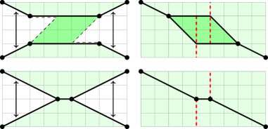
Figure 6. Surgery to make $\operatorname{IAS}^{2}$ into $P\cup P^{\rm opp}$: $(\ell^{\prime}_{i-1},\ell^{\prime}_{i},\ell^{\prime}_{i+1})=(1,5,1)\to(\ell_{i-1},\ell_{i},\ell_{i+1})=(2,1,2)$

As in Prop. 4.6, let $L=\pi^{*}L_{\widehat{Y}}$ for some ample ${\mathbb{Q}}$-line bundle on ${\widehat{Y}}$. We modify $L_{\widehat{Y}}$ by considering an ample ${\mathbb{Q}}$-line bundle $L^{\prime}_{\widehat{Y}}=L_{\widehat{Y}}-\sum_{i=1}^{k}c_{i}E_{i}$ for some small positive rational numbers $0<c_{i}\ll 1$. Here, $E_{i}$ are the $k$ $(-4)$-curves. Below, we consider the case of a single $(-4)$-curve $E_{i}$, with obvious modifications for the general case. Let $\ell_{i}=L_{\widehat{Y}}\cdot E_{i}$ and $\ell^{\prime}_{i}=L^{\prime}_{\widehat{Y}}\cdot E_{i}$. Then $\ell_{i}=\ell^{\prime}_{i}-4c_{i}$ and $\ell_{i\pm 1}=\ell^{\prime}_{i\pm 1}+c_{i}$.

We consider the polarization ${\mathcal{O}}(\ell_{i},c_{i})$ on $Z_{i}={\mathbb{P}}^{1}\times{\mathbb{P}}^{1}$. The Symington polytope is obtained from a parallelogram with sides of lattice length $\ell_{i}^{\prime}$ and $c_{i}$ by cutting two triangles of side $c_{i}$ erasing two of the four sides, as in the first picture of Fig. 6. This produces an $\operatorname{IAS}^{2}$ as in the second picture (going clockwise) with two $I_{1}$ singularities off the equator. Node sliding each of them by lattice distance $c_{i}$ gives the $\operatorname{IAS}^{2}$ $B=P\cup P^{\rm opp}$ with sides $\ell_{i}$ and $2k$ $I_{1}$ singularities on the equator. The effect of this nodal slide on the lengths is $(\ell^{\prime}_{i-1},\ell^{\prime}_{i},\ell^{\prime}_{i+1})\to(\ell^{\prime}_{i-1}+c_{i},\ell^{\prime}_{i}-4c_{i},\ell^{\prime}_{i+1}+c_{i})$, and gives the symplectic form corresponding to $L_{\widehat{Y}}$.

General case. We use the reduction given in Corollary 4.13 and Lemma 4.17. Let ${\widehat{X}}$, ${\widehat{X}}_{1}$ be K3 surfaces as in Lemma 4.17. Vary the ${\mathbb{Q}}$-line bundle $L$ on ${\widehat{X}}$ continuously until it becomes zero on the $(-2)$-curve $E$ and gives a contraction ${\widehat{X}}\to{\widehat{X}}^{\prime}$ to a K3 surface with a node. This produces a continuous family of integral affine structures. In the limiting integral-affine structure on $B$, two $I_{1}$ singularities with monodromy rays parallel to the equatorial edge collide to give an $I_{2}$ singularity with the monodromy ray in the same direction. Smoothing ${\widehat{X}}^{\prime}$ to a surface ${\widehat{X}}_{1}$ in the ${\widehat{S}}_{1}$ family gives a Lagrangian torus fibration $\mu\colon{\widehat{X}}_{1}\to B$ with same $B$. We repeat this procedure $(g-1)$ times to complete the proof.

One can produce either $2(g-1)$ $I_{1}$ singularities in this way, or a single $I_{2(g-1)}$ singularity, they are equivalent up to nodal slides along the equator. ∎

Example 7.5 (An $\operatorname{IAS}^{2}$ for ${\widehat{S}}=(12,6,1)$).

Let $(\overline{{\overline{V}}},\overline{{\overline{D}}})=({\mathbb{P}}^{2},L_{1}+L_{2}+L_{3})$ be a toric anticanonical pair with the $L_{i}$ lines forming a triangle. Let $({\overline{V}},{\overline{D}})\to(\overline{{\overline{V}}},\overline{{\overline{D}}})$ be the blow up at the three corners of the triangle, introducing three exceptional classes $e_{1}$, $e_{2}$, $e_{3}$ to get a Cremona surface. Then, let $(V^{\prime},D^{\prime})\to({\overline{V}},{\overline{D}})$ be the blow up of $9$ total points, $3$ on each strict transform of $L_{i}$, with exceptional classes $e_{4},\,\dots,\,e_{12}$.

The pair $(V^{\prime},D^{\prime})$ arises as an $I_{6}I_{0}$ type quotient of an elliptic K3 surface, as in Theorem 4.1, with the length $6$ cycle $D^{\prime}$ of alternating $(-1)$- and $(-4)$-curves representing the quotient of the $I_{6}$ cycle. Hence $(V^{\prime},D^{\prime})$ is the quotient of an elliptic K3 surface with involution, with generic Picard group $(13,7,1)$.

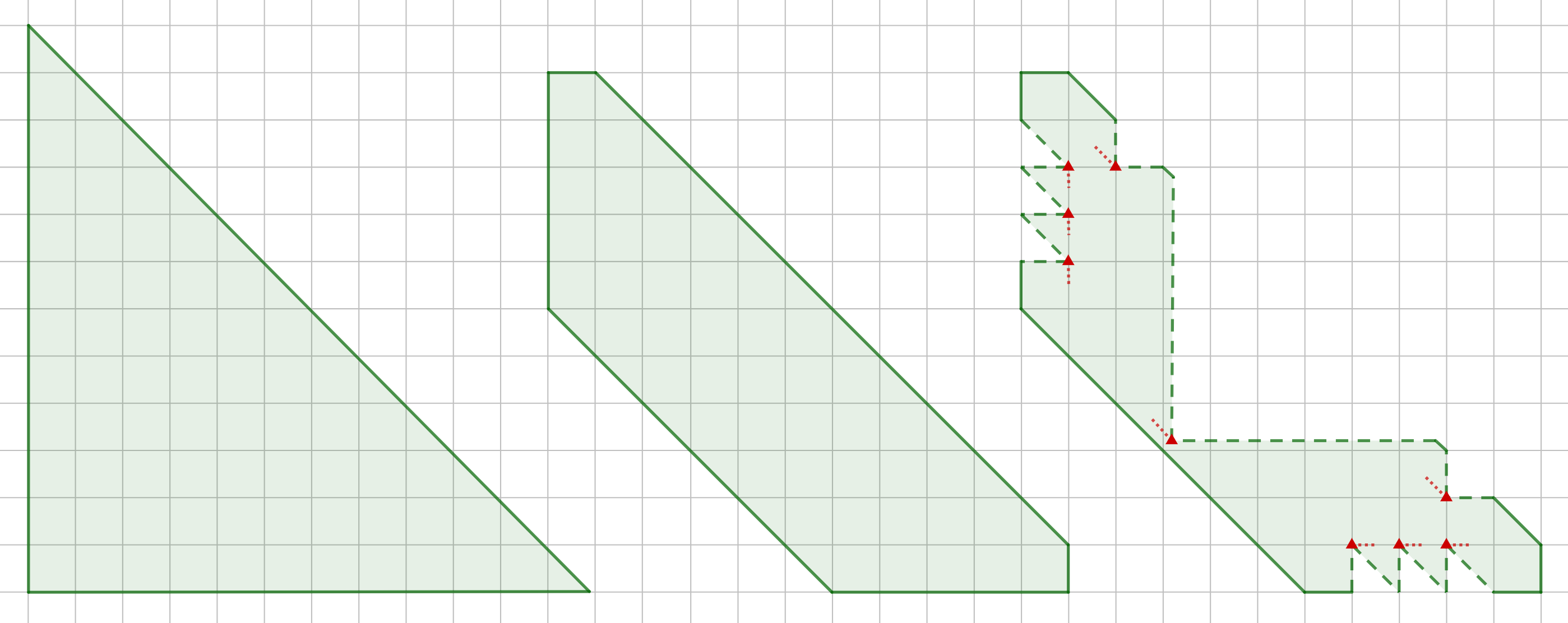
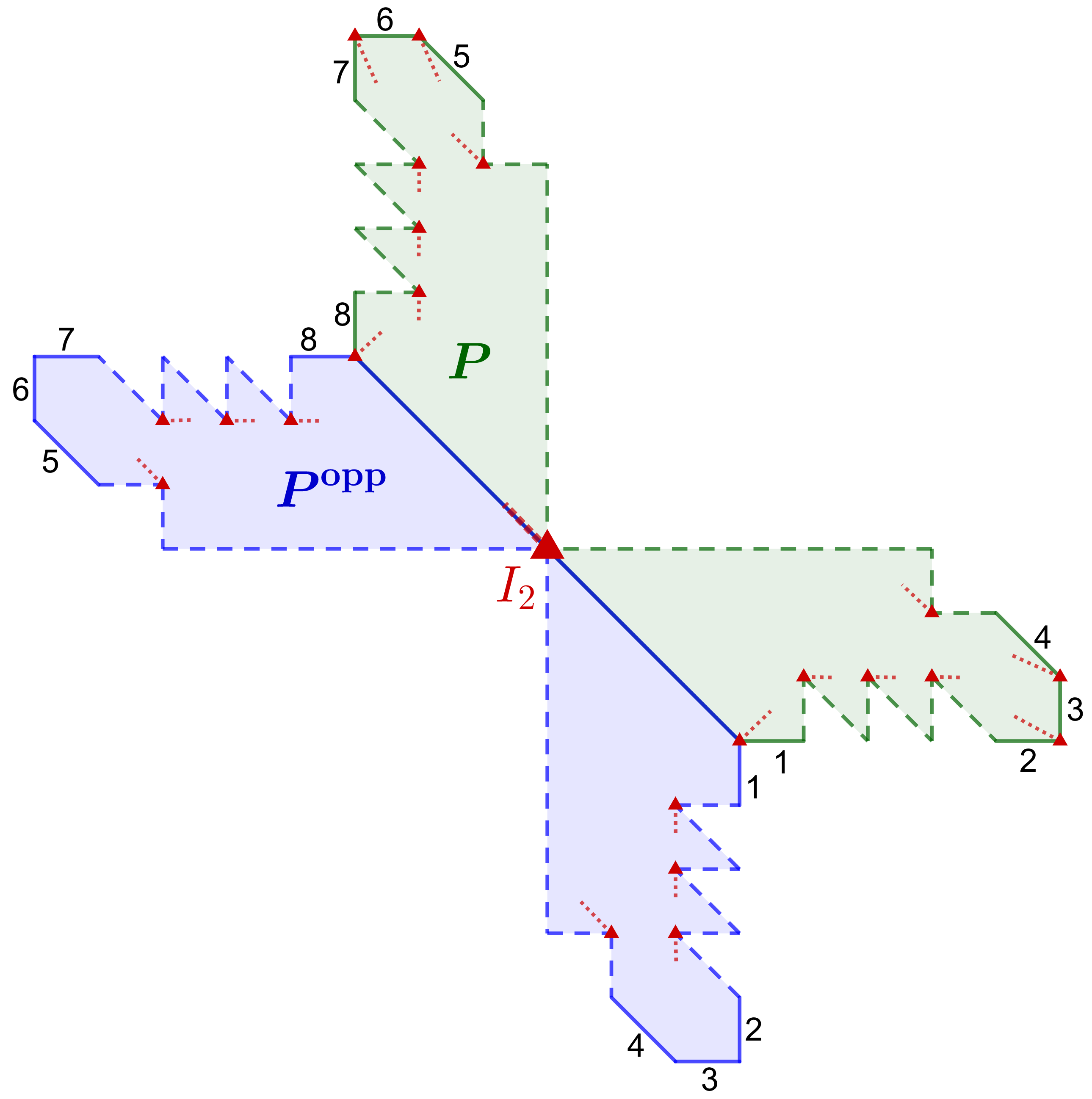
Figure 7. Left: the moment polytope for $(\mathbb{P}^{2},12h)$. Center: the moment polytope for $(Bl_{p_{1},p_{2},p_{3}}{\mathbb{P}}^{2},12h-6e_{1}-e_{2}-e_{3})$. Right: the Symington polytope for $(Bl_{p_{1},\cdots,p_{12}}{\mathbb{P}}^{2},L_{\epsilon})$.

Figure 8. An integral-affine sphere associated to an ample class in ${\widehat{S}}=(12,6,1).$ There are $22$ $I_{1}$ singularities and $1$ $I_{2}$ singularity.

Consider the ample class $12h$ on $\overline{{\overline{V}}}={\mathbb{P}}^{2}$. After the three corner blow-ups, we have an ample class $12h-6e_{1}-e_{2}-e_{3}$ on ${\overline{V}}$. Their moment polytopes are depicted in the left and center of Figure 8. After the next nine interior blow-ups, we have an ample class

$$L_{\epsilon}:=12h-6e_{1}-(6-\epsilon)e_{8}-\sum_{i\geq 2,\,i\neq 6}e_{i}$$

on $(V^{\prime},D^{\prime})$ whose corresponding Symington polytope $P$ is shown on the right of Figure 8. As $\epsilon\to 0$, this class becomes only big and nef, because $L_{\epsilon}\cdot(h-e_{1}-e_{8})=\epsilon$ and $h-e_{1}-e_{8}$ represents the class of an exceptional curve. Thus, $L_{0}$ represents an ample class on the pair $(V,D)\leftarrow(V^{\prime},D^{\prime})$ resulting from the blow-down of $h-e_{1}-e_{8}$. Set $({\widehat{Y}},D)=(V,D)$. Then ${\widehat{Y}}$ is the quotient of a K3 surface ${\widehat{X}}$ with generic Picard group $(12,6,1)$, or alternatively $k=3$, $g=2$.

We glue two copies $B=P\cup P^{\rm opp}$ together along their common boundary to form a sphere, and let $\epsilon\to 0$. At $\epsilon=0$, the two $I_{1}$ singularities in $P$ and $P^{\rm opp}$ collide to form an $I_{2}$ singularity on the equator. See Figure 8.

As in Lemma 7.1, we have a degeneration $({\widehat{X}}^{\prime},L)\to(C,0)$ of K3 surface with involution, where ${\widehat{X}}_{0}^{\prime}=V^{\prime}\cup_{D^{\prime}}V^{\prime}$ and the generic Picard lattice is ${\widehat{S}}^{\prime}=(13,7,1)$, and with $L\big{|}_{{\widehat{X}}_{0}^{\prime}}=(L_{\epsilon},L_{\epsilon})$. At $\epsilon=0$, the class $L$ is only big and nef on the general fiber, contracting the $(-2)$-curve which results from smoothing the union of $h-e_{1}-e_{8}$ and its opposite. But instead smoothing ${\widehat{X}}_{0}^{\prime}$ into the larger moduli space $(12,6,1)$, we get a degeneration ${\widehat{X}}$ for which the class $L$ is ample on the general fiber. By Theorem 7.4, we have a Lagrangian torus fibration ${\widehat{X}}_{t}\to B$, and as predicted, there $2k=6$ $I_{1}$ singularities on the equator with monodromies transverse to the equator, and there is one $I_{2(g-1)}=I_{2}$ singularity on the equator, with monodromy parallel to it. As in Corollary 4.13, the $(12,6,1)$ lattice was reached by a single $(-1,-1)$ Heegner move $(13,7,1)\rightarrowtail(12,6,1)$, corresponding a white vertex of the $(13,7,1)$ Coxeter diagram attached to the outer $6$-cycle by a bolded edge (see Fig. 3).

7C. Mirror symmetry and involutions

Let $\mu\colon{\widehat{X}}\to B=P\cup P^{\rm opp}$ be the Lagrangian torus fibration of Theorem 7.4, associated to some $2$-elementary lattice ${\widehat{S}}$. Suppose that the same $B=\Gamma(X_{0})$ is the $\operatorname{IAS}^{2}$ obtained as in Construction 6.15, from the dual complex of a Kulikov surface $X_{0}$. We may smooth $X_{0}$ to a Kulikov model $X\to(C,0)$. By the results of the following section, whenever ${\widehat{S}}={\overline{T}}=e^{\perp}/e$ is the target of a mirror move from $S$, we may choosing the gluings of $X_{0}$ appropriately so that $X\to(C,0)$ admits an involution acting on $\Gamma(X_{0})=B$ by the specified one, exchanging $P$ and $P^{\rm opp}$, with generic Picard group $S$.

By the Mirror Theorem 6.19 there is a diffeomorphism $\phi\colon{\widehat{X}}\to X_{t}$ inducing an identification between a nef class $L\in\hat{e}^{\perp}/\hat{e}$ on ${\widehat{X}}$ and the monodromy vector $\lambda\in{\overline{T}}=e^{\perp}/e$. Now on ${\widehat{X}}$ there are two involutions: $\hat{\iota}$ and $\iota_{\phi}:=\phi^{-1}\circ\iota\circ\phi$.

Theorem 7.6.

The two involutions $\hat{\iota}$ and $\iota_{\phi}$ differ by negation (with respect to some section) $z\to-z$ in the generic fiber $\hat{e}\simeq(S^{1})^{2}$ of $\mu$, composed with a translation in the fibers. The diffeomorphism $\phi$ identifies $(e^{\perp}/e)^{+}$ with $(\hat{e}^{\perp}/\hat{e})^{-}$ and $(e^{\perp}/e)^{-}$ with $(\hat{e}^{\perp}/\hat{e})^{+}$.

Proof.

The Mirror Theorem [EF21, Prop. 3.14] proceeds by identifying ${\widehat{X}}$ and $X_{t}$ as isomorphic torus bundles over the same base $B$ (this is essentially topological SYZ mirror symmetry). The torus bundle on ${\widehat{X}}$ is the Lagrangian torus fibration $\mu$, and Proposition 6.17 serves to construct the Lagrangian torus fibration on $X_{t}$ as the composition of a Clemens collapse, and almost toric fibrations of components $V_{i}\subset X_{0}$ (note that our fibration $\mu$ was also constructed this way, but from a different Kulikov model ${\widehat{X}}_{0}={\widehat{Y}}\cup_{D}{\widehat{Y}}$). Since the smoothing $X\to(C,0)$ extends an involution on $X_{0}$, we can make the Clemens collapse and almost toric fibrations involution equivariant, and so can ensure both $\iota$ and the diffeomorphism $\phi$ respect the torus bundle structure over $B$.

Thus, $\hat{\iota}$ and $\iota_{\phi}$ respect the torus bundle structure, and define the same involution on the base $B$, exchanging $P$ and $P^{\rm opp}$. So the composition $\iota_{\phi}\circ\hat{\iota}^{-1}$ is a fiber-preserving diffeomorphism of the torus bundle, and defines an element of the mapping class group $\operatorname{GL}(2,{\mathbb{Z}})$ of the general fiber. Since not all of the monodromy rays of the singularities of $B$ are parallel, the only element centralizing the monodromy on $S^{2}\setminus\{p_{i}\}$ is $\pm{\rm id}$.

So $\iota_{\phi}\circ\hat{\iota}$ must give $\pm{\rm id}$ in the mapping class group of the general fiber. By the Mirror Theorem, $\phi$ exchanges the class $L\in S$ of an ample line bundle in the $(+1)$-eigenspace of $\iota$ with the monodromy invariant $\lambda\in{\widehat{S}}={\overline{T}}$, which is in the $(-1)$-eigenspace of $\hat{\iota}$. Thus, $\iota_{\phi}\circ\hat{\iota}=-{\rm id}$ composed with a translation. The negation $z\to-z$ in the torus fibers acts by multiplication by $(-1)$ on $\hat{e}^{\perp}/\hat{e}$, as can be seen e.g. from the Leray spectral sequence $H^{p}(B,R^{q}\mu_{*}\underline{{\mathbb{Z}}})\implies H^{p+q}({\widehat{X}},\underline{{\mathbb{Z}}})$. The eigenspaces of $\hat{\iota}$ and $-\hat{\iota}$ are opposite of each other. A translation in the fibers acts on $\hat{e}^{\perp}/\hat{e}$ as identity. The theorem follows. ∎

8. Kulikov models of K3 surfaces with a nonsymplectic involution

In this section for each of the $75$ lattices of Fig. 1 we construct a family of models $(X,R)$ adapted to the ramification divisor of the involution. Moreover, for the $50$ cases when $R$ contains a curve $C_{g}$ with $g\geq 2$, we construct the divisor models $(X,C_{g})$. We do it first for a generic $\lambda$ in the interior of the fundamental domain ${\mathfrak{C}}_{2}$, and then in Sections 8G, 8H for $\lambda$ on a face of ${\mathfrak{C}}_{2}$.

8A. The main construction

Let $S$ be a lattice from Fig. 1, $e\in T$ a $0$-cusp, and ${\overline{T}}=e^{\perp}/e$. Let $\lambda\in{\overline{T}}\cap{\mathcal{C}}$ be a monodromy invariant. Recall that ${\mathcal{C}}$ is the positive cone. Our goal now is to explicitly construct a Type III $d$-semistable Kulikov surface $X_{0}$ with the monodromy invariant $\lambda$, admitting an involution $\iota_{0}$ which extends to an involution on a Kulikov model $X\to(C,0)$ for which $X_{t}\in F_{S}$.

Proposition 8.1.

For $g\geq 2$, $S\neq(10,8,0)$, and for all $0$-cusps of $F_{S}$, there is a well-defined stratum function

$${\mathbb{S}}\colon\{\lambda\colon{\overline{T}}\cap{\mathcal{C}}\}\to\{\textrm{combinatorial types of KSBA-stable surfaces}\}$$

which assigns to each monodromy invariant $\lambda$ of a Type III degeneration, the combinatorial type of the stable limit of a degeneration $({\overline{X}},\epsilon{\overline{C}}_{g})$, whose monodromy is $\lambda$. Furthermore, the loci on which ${\mathbb{S}}$ is locally constant form the cones of a semifan $\mathfrak{F}$ for which $({\overline{F}}_{S})^{\nu}={\overline{F}}_{S}^{\mathfrak{F}}$.

Dropping the condition on $g$, we have that any degeneration with monodromy invariant $\lambda$ admits a Kulikov model of fixed combinatorial type, adapted to $R$.

Recall, the Kulikov model is adapted to $R$ if the flat limit contains no strata, and any components of positive genus have a nef limit.

Proof.

It is already a consequence of the general theory, see [AE21, Thm. 1], [AEH21, Thm. 3.24], that when $g\geq 2$, the KSBA compactification ${\overline{F}}_{S}$ is normalized by a semitoroidal compactification associated to some semifan $\mathfrak{F}$. This is because the fixed locus of an involution is a so-called “recognizable divisor.”

The main tool to find the associated semifan is [AE21, Thm. 9.3]. It states that the cones $\sigma$ of the semifan $\mathfrak{F}$ are determined as the (closures of) collections of monodromy invariants $\lambda\in\sigma$ for which the KSBA-stable model of a degeneration with monodromy invariant $\lambda$ has a fixed combinatorial type, see [AE21, Def. 8.12]. Furthermore, recognizability ensures that any degeneration with a given monodromy invariant in the projective class of $\lambda$ has the same combinatorial type [AE21, Cor. 8.13]. The first statement follows.

Even when $R$ contains no components of genus $g\geq 2$, many of the same properties of recognizability hold, in particular, the existence of a combinatorially constant Kulikov model adapted to $R$ for all divisors with a fixed monodromy invariant $\lambda$. Specifically, the second statement follows from [AE21, Prop. 8.16] and the arguments in [AEH21, Thm. 3.24]. ∎

With these results in mind, we need only construct some generic divisor model with monodromy invariant $m\lambda$, for all $\lambda\in{\overline{T}}\cap{\mathcal{C}}$, and identify when the combinatorial type of the stable model changes (as a function of $\lambda$).

It is sufficient to consider $\lambda$ up to the isometry group $O({\overline{T}})$. Thus, we can take $\lambda$ in a fundamental chamber ${\mathfrak{C}}_{2}$ for the reflection group $W_{2}$ or, more economically, in a fundamental chamber ${\mathfrak{C}}_{\rm r}$ for the full reflection group $W_{\rm r}$. We only care about a generic $X_{0}$ within its combinatorial type. This is quite useful, as even a smooth, non-generic K3 surface $X_{0}\in\Delta\subset{\mathbb{D}}_{S}$ does not smooth with its involution into $F_{S}$.

Now we set ${\widehat{S}}={\overline{T}}$ and consider the family of K3 surfaces with the generic Picard lattice ${\widehat{S}}$. Let ${\widehat{X}}$ be one such surface with an involution $\hat{\iota}$. We have $(\operatorname{Pic}{\widehat{X}})^{+}={\widehat{S}}$. By Theorem 7.4, for an ample line bundle $L$ on ${\widehat{X}}$ there exists a Lagrangian torus fibration $\mu\colon({\widehat{X}},\omega)\to B$ with $B$ an $\operatorname{IAS}^{2}$ of a special type: $B=P\cup P^{\rm opp}$, a union of two Symington polytopes interchanged by the involution $\hat{\iota}$, and $[\omega]=L$.

By Lemma 4.3 and Proposition 4.6, assuming $S\neq(10,10,0)$, ${\mathfrak{C}}_{\rm r}$ can be identified with $(\operatorname{Nef}{\widehat{X}})\cap{\widehat{S}}_{\mathbb{R}}=\operatorname{Nef}{\widehat{Y}}$ for a particular quite degenerate rational surface ${\widehat{Y}}$, so that $L=\pi^{*}L_{\widehat{Y}}$. Replacing $L$ by $2L$ we can assume $L_{\widehat{Y}}$ to be integral. Alternatively, we can work with a generic K3 surface in the ${\widehat{S}}$-family and identify ${\mathfrak{C}}_{2}\simeq(\operatorname{Nef}{\widehat{X}})\cap{\widehat{S}}_{\mathbb{R}}=\operatorname{Nef}{\widehat{Y}}$. Working with ${\mathfrak{C}}_{2}$ or ${\mathfrak{C}}_{\rm r}$ is purely a matter a convenience, except for $S=(17,3,1)$ where we only computed ${\mathfrak{C}}_{2}$ and not ${\mathfrak{C}}_{\rm r}$ in Section 3E.

Next, pick a triangulation ${\mathcal{T}}$ of $B$ into unit lattice volume triangles, in such a way that: the vertices are lattice points, ${\mathcal{T}}$ is involution-invariant, and the edges contain the equator. For instance, such a triangulation arises from triangulating $P$ entirely. Now interpret $(B,{\mathcal{T}})$ as an $\operatorname{IAS}^{2}$ coming from a Type III surface $X_{0}$ via Construction 6.15. That is, $B=\Gamma(X_{0})$ and for each vertex of ${\mathcal{T}}$, we have an anticanonical pair $(V_{i},D_{i})$ whose pseudofan ${\mathfrak{F}}(V_{i},D_{i})$ models the star of the vertex. Then, we glue $X_{0}=\cup V_{i}$ along $D_{i}$ according to the triangulation.

For a fixed such $B$ with triangulation, the family of $d$-semistable Type III surfaces $X_{0}$ satisfying $\Gamma(X_{0})=B$ is $({\mathbb{C}}^{*})^{19}=\operatorname{Hom}(\Lambda,{\mathbb{C}}^{*})$. Here, $\Lambda$ can be computed directly from $X_{0}$ by Eq. (4). We have $\Lambda=\lambda^{\perp}$ in $e^{\perp}/e\simeq L_{\rm IAS}={\rm II}_{2,18}$, where $e$ corresponds to the $0$-cusp into which $0\in C$ maps via the extension of the period map, and $\lambda$ is the monodromy invariant.

Example 8.2.

Taking $B=P\cup P^{\rm opp}$ from Figure 8, we may triangulate it in an involution-invariant manner, and realize it as the dual complex of a Type III Kulikov surface. See Figure 9. Then $22$ components $(V_{i},D_{i})$ have charge $Q(V_{i},D_{i})=1$, one component has $Q=2$, and the remaining components, with $Q=0$, are toric.

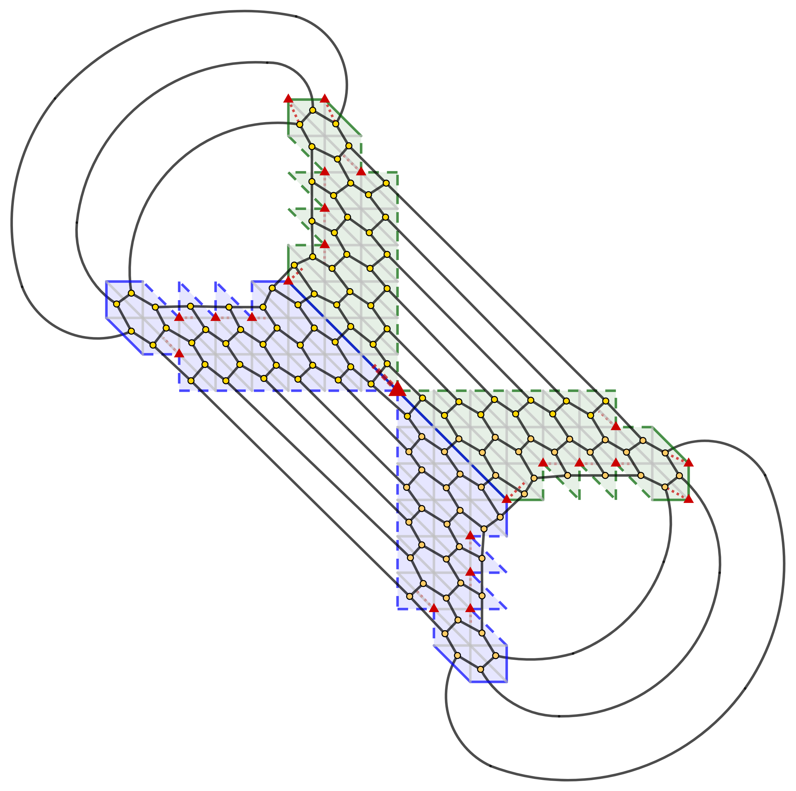
Figure 9. A Kulikov surface $X_{0}$ for ${\widehat{S}}=(12,6,1)$ with $\Gamma(X_{0})=B$, with triple points shown in yellow and double curves in black.

Theorem 8.3.

Let $S\leadsto{\overline{T}}\simeq{\widehat{S}}$ be a mirror move let $L\in{\widehat{S}}$ be an ample line bundle on ${\widehat{X}}\in{\widehat{S}}$. Let $\lambda=L$ under the identification ${\overline{T}}\simeq{\widehat{S}}$. Let $P$ be the Symington polytope of ${\widehat{Y}}={\widehat{X}}/\hat{\iota}$ associated to the image $L_{\widehat{Y}}$ and let $B=P\cup P^{\rm opp}$ be the integral-affine sphere built from gluing two copies of $P$ (see Section 8B for further details on these gluings). Let ${\mathcal{T}}$ be an involution-invariant triangulation of $B$ containing the equator.

Then $B=\Gamma(X_{0})$ for a Type III Kulikov surface $X_{0}$ admitting an involution $\iota_{0}$ inducing the involution on $B$. Furthermore, by choosing the period of $X_{0}$ appropriately, there is a smoothing $X\to(C,0)$ with involution $\iota$ whose general fiber $X_{t}$ lies in $F_{S}$ and whose monodromy invariant is $\lambda\in{\overline{T}}$.

It is worth remarking that the combinatorial type of $X_{0}$ is completely determined by the vector $\lambda\in{\overline{T}}$ and has nothing to do with the source $S$ of the mirror move. This source $S$ is determined by choosing the period $\psi_{X_{0}}$ appropriately.

Proof.

We observe that the gluings of the standard surface $X_{0}$ (satisfying $\psi_{X_{0}}=1$) are unique, hence invariant under the involution on $B$. So $X_{0}$ admits an involution $\iota_{0}$ acting on $B$ by the involution $\iota_{\rm IAS}$ switching $P$ and $P^{\rm opp}$.

We analyze the deformations $X_{0}\rightarrowtail X_{0}^{\prime}$ for which $X_{0}^{\prime}$ retains an involution $\iota_{0}^{\prime}$. For there to be an involution on $X_{0}^{\prime}$ the period point $\psi_{X_{0}^{\prime}}\in\operatorname{Hom}(\Lambda,{\mathbb{C}}^{*})$ must be anti-invariant with respect to $\iota_{0}^{*}$, under identification $\Lambda(X_{0}^{\prime})\simeq\Lambda(X_{0})$. This is because the target ${\mathbb{C}}^{*}$ depends on a choice of orientation on $B$, which is reversed by $\iota_{\rm IAS}$, see [AET19, Sec. 6G]. We conclude that a generic involutive $X_{0}^{\prime}$ deforming $X_{0}$ is one for which ${\rm ker}(\psi_{X_{0}^{\prime}})\supset\Lambda^{+}$ where $\Lambda^{+}$ is the $(+1)$-eigenspace of $\iota_{0}^{*}$ acting on $\Lambda(X_{0})$. The period torus for these involutive Kulikov surfaces is ${\rm Hom}(\Lambda/\Lambda^{+},{\mathbb{C}}^{*})$. These deformations of the standard surface $X_{0}$ will become the Kulikov surfaces corresponding to a simple mirror move $S\to{\widehat{S}}$.

The involution $\iota_{\rm IAS}$ on $B$ has an induced action $\iota_{\rm IAS}^{*}$ on $H^{1}(B,T_{\mathbb{Z}}^{*})\simeq{\rm II}_{2,18}=L_{\rm IAS}$ which is easily seen to be an isometry with respect to the intersection form [ABE22, Ex. 7.27] on visible curves, see Section 6G. The induced involution on $\Lambda=\lambda^{\perp}$ agrees with the action of $\iota_{0}^{*}$ on $\Lambda(X_{0})$ for the standard surface $X_{0}$. Here $\lambda$, too, can be interpreted purely in integral-affine terms as the so-called radiance obstruction in $H^{1}(B,T_{\mathbb{Z}}^{*})$ of the integral-affine structure. So it is automatically preserved by $\iota_{\rm IAS}$. We define $\rho_{\rm IAS}:=-\iota_{\rm IAS}^{*}\in O(L_{\rm IAS})$. The motivation for this definition is Theorem 7.6 (which notably relies on this theorem).

Let $L_{\rm IAS}^{\pm}$ denote the eigenspaces of $\rho_{\rm IAS}$. We claim that $L_{\rm IAS}^{-}={\widehat{S}}$ or equivalently $(\iota_{\rm IAS}^{*})^{+}={\widehat{S}}$. This can be verified purely on the symplectic side, by observing that we have an isomorphism $\hat{e}^{\perp}/\hat{e}\cong L_{\rm IAS}$ where $\hat{e}$ is the Lagrangian fiber class of $\mu\colon{\widehat{X}}\to B$. The involution $\hat{\iota}$ quotients this fibration of ${\widehat{X}}$ to the Lagrangian torus fibration ${\widehat{Y}}\to P$. Thus, $L_{\rm IAS}^{-}\otimes{\mathbb{Q}}\simeq H^{2}(Y,{\mathbb{Q}})$ and so ${\widehat{S}}\subset\hat{e}^{\perp}/\hat{e}$ must equal $L_{\rm IAS}^{-}$.

Denote $L_{\rm IAS}^{+}:=S^{\rm sat}$ (this choice of notation will be made reasonable soon). It is a $2$-elementary lattice in $L_{\rm IAS}\simeq{\rm II}_{2,18}$ perpendicular to ${\widehat{S}}$ and so $S^{\rm sat}$ is the source of a simple mirror move with target ${\widehat{S}}$. Smoothing $X_{0}^{\prime}$ (a deformation of the standard surface $X_{0}$ as above), keeping the classes in $S^{\rm sat}$ Cartier, we produce the claimed degeneration of the theorem, in the case of a simple mirror move. The smoothings that keep $S^{\rm sat}$ Cartier (at least for $X_{0}^{\prime}$ period-generic) are identified with the deformations extending the involution $\iota_{0}$ by [AET19, Thm. 6.35].

For the non-simple mirrors, we observe that an involutive $X_{0}$ need not be a deformation of the standard surface: There may be other connected components in ${\rm Hom}(\Lambda,{\mathbb{C}}^{*})$ of the space of anti-invariant periods. These connected components also admit an involution, because

1. $\rho_{\rm IAS}$ acts on the (re)gluing complex of [AE21, Sec. 7A] and an involution anti-invariant regluing of an involutive $X_{0}$ will be involutive, and

2. the period and gluing complexes are quasi-isomorphic [AE21, Thm. 7.9].

The connected components of the anti-invariant periods are determined by a lattice $S=({\ker\psi})^{+}$ which has index at most $2$ in $S^{\rm sat}=L_{\rm IAS}^{+}$ and furthermore contains $(1+\rho_{\rm IAS})L_{\rm IAS}^{+}$. Up to isometry, these are in bijection with the sources $S$ of mirror moves with target ${\widehat{S}}$, by Theorem 5.16.

So these components of anti-invariant periods also parameterize involutive Kulikov surfaces, and the same argument as in the previous paragraph applies to prove that such an $X_{0}^{\prime}$ smooths, with its involution, into moduli of $S$-polarized K3 surfaces.

Finally, we must verify that the monodromy invariant $\lambda$ is as stated. This is follows from the Monodromy Theorem 6.19, which identifies $[\omega]=L\in\hat{e}^{\perp}/\hat{e}$ on ${\widehat{X}}$ with $\lambda\in e^{\perp}/e$ on the smoothing $X_{t}^{\prime}$ of $X_{0}^{\prime}$. ∎

By Proposition 8.1, we must understand the stable models associated to each $\lambda\in{\mathfrak{C}}_{2}$ (including for $\lambda$ only big and nef, on faces of ${\mathfrak{C}}_{2}$). For this, it will suffice to show that the Kulikov models of Theorem 8.3 are, after some appropriate M1 modifications (Section 8D), adapted to $R$. Then, by passing to the stable model (6.9), we can explicitly determine the combinatorial types of stable models on each face of ${\mathfrak{C}}_{2}$ in terms of the ADE surfaces of [AT21] to find the semifan ${\mathfrak{F}}$.

This requires understanding in some detail how the singularities on the $\operatorname{IAS}^{2}$ collide. When $\lambda=L$ is ample, in the interior of ${\mathfrak{C}}_{2}$, the parameters $\ell_{i}:=\lambda\cdot\alpha_{i}$ are all positive, where $\alpha_{i}$ are the simple roots. Then, no singularities $B(\lambda)$ have collided, except the $I_{2g-2}$ singularity which forms on an edge of the equator.

For a non-general $\lambda$ with $\lambda^{2}>0$ lying on a face of ${\mathfrak{C}}_{2}$, some $\ell_{i}=0$. The corresponding $\operatorname{IAS}^{2}$ $B(\lambda)$ is obtained from a generic $\operatorname{IAS}^{2}$ $B(\lambda+t\lambda_{0})$ for some $\lambda_{0}\in({\mathfrak{C}}_{2})^{\rm int}$ in the interior, by letting $t\to 0$. Then, the $I_{1}$ and $I_{2g-2}$ singularities on $B(\lambda+t\lambda_{0})$ collide as $t\to 0$ to give more complicated singularities associated to higher charge anticanonical pairs $(V_{i},D_{i})$. We discuss this in Section 8G.

Ultimately, only the facets of ${\mathfrak{C}}_{\rm r}$ which are also facets of ${\mathfrak{C}}_{2}$ matter; for the other facets, the singularity collision can be avoided, and the stable models will not change. For the (highly non-generic) $\lambda\in{\mathfrak{C}}_{\rm r}$ satisfying $\lambda^{2}=0$, the $\operatorname{IAS}^{2}$ collapses to an interval, the dual graph of a Type II degeneration. These are discussed in Section 8H.

8B. Edge behavior in the gluing of $P$ and $P^{\rm opp}$

Consider an $\operatorname{IAS}^{2}$ $B=P\cup P^{\rm opp}$ with a set of integral points and an involution $\iota$ exchanging $P$ and $P^{\rm opp}$. Let $C$ be a side of $P$. The gluing along $C$ could be of two types. We say that it is even if for any lattice point $u\in P$ the lattice distance between $u$ and $\iota(u)$ is always even, and odd if it is odd for some $u$. This is illustrated in Fig. 10.

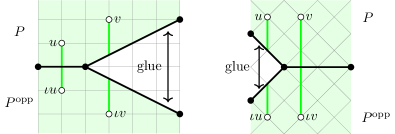
Figure 10. Equatorial behavior: even vs odd

Lemma 8.4.

In the $I_{2\bar{k}}I_{0}$ case, when $B$ has $2\bar{k}>0$ $I_{1}$ singularities on the equator at the vertices of $P$, gluing along the side corresponding to a curve $E_{i}$ on ${\widehat{Y}}$ with $E_{i}^{2}=-4$ (resp. $E_{i}^{2}=-1$) is even (resp. odd).

Proof.

The statement is obvious from Fig. 6. ∎

Note: when there are no singularities on the equator, there are no such restrictions and below we will give examples of both even and odd behaviors.

Next, we find anticanonical pairs $(V,D)$ corresponding to the nonsingular lattice points of $B$ on the equator. Nonsingularity implies means that these are toric pairs. We say that an involution on a toric pair is nonsymplectic if the action on the cocharacter lattice ${\mathbb{Z}}^{2}$ has determinant $-1$. Equivalently, it acts by multiplying a generator of $H^{0}(V,\omega_{V}(D))$ by $-1$.

Lemma 8.5.

Let $\iota$ be a nonsymplectic involution on a toric pair $(V,D)$ such that the fixed locus $V^{\iota}$ does not contain any torus-fixed points of $V$. Then $V$ admits a generic ruling $\pi\colon V\to{\mathbb{P}}^{1}$ with two sections $s_{1}$, $s_{2}$. The map commutes with a nontrivial involution on the base ${\mathbb{P}}^{1}$ and there are three cases:

1. $V^{\iota}$ consists of four points, two on each $s_{i}$.

2. $V^{\iota}$ is a fiber of $\pi$ plus two points, one on each $s_{i}$.

3. $V^{\iota}$ is two fibers of $\pi$.

The cases E0 and E2 give the even equatorial behavior, and E1 the odd equatorial behavior. The fan of $V$ is an involution-invariant subdivision of the fan for ${\mathbb{F}}_{n}$ with $n$ even for E0, E2, resp. with $n$ odd for E1.

Proof.

Consider the fan ${\mathfrak{F}}$ of $V$. The involution acting on the cocharacter lattice $N={\mathbb{Z}}^{2}$ has a fixed line and it does not intersect the interior of a two-dimensional cone in ${\mathfrak{F}}$ by the condition on $V^{\iota}$. So in ${\mathfrak{F}}$ there are two rays $\pm e_{1}$, fixed by the involution. Let $\langle e_{1},e_{2}\rangle$ be a basis. Then $e_{2}\to-e_{2}+ke_{1}$ with $k$ either even or odd, and we can assume that $k=0$ or $1$. Any nonsingular involution-invariant fan is a symmetric subdivision of the fan with the rays $\pm e_{1}$, $e_{2}+me_{1}$, $-e_{2}+(k+m)e_{1}$ which is the fan of ${\mathbb{F}}_{n}$ for $n=|k+2m|$. This defines the action on monomials up to constants: $x^{m}\to c(m)x^{\iota m}$. It is easy to see that up to rescaling there are the following three possibilities, giving the three cases above: (E0) $(x,y)\to(-x,y^{-1})$, or (E1) $(x,y)\to(x,xy^{-1})$, or (E2) $(x,y)\to(x,y^{-1})$. ∎

We begin by describing Kulikov models for the lattices ${\overline{T}}$ on the $\bar{g}=1$ line. Note that these only appear as the targets of simple mirror moves.

8C. Models for ${\overline{T}}=(10+\bar{k},10-\bar{k},\delta)$, $1\leq\bar{k}\leq 9$

By Theorem 7.4, for an ample line bundle $L$, i.e. a generic monodromy vector $\lambda$, the $\operatorname{IAS}^{2}$ $B$ has $24$ distinct $I_{1}$ singularities. Consider the Type III surface $X_{0}$ of Theorem 8.3 with its involution $\iota_{0}$ and involution-equivariant smoothing $(X,\iota)$. The flat limit of $R_{t}={\rm Fix}(\iota_{t})$ is the divisorial locus $R_{0}$ in ${\rm Fix}(\iota_{0})$. Note that since $X$ is smooth, ${\rm Fix}(\iota)$ as a set consists of relative curves $R\subset X$ and isolated points in $X_{0}$.

Let us first deal with the pairs $(V_{j},D_{j})$ corresponding to the lattice points in the interior of either hemisphere. They fall into disjoint pairs $V_{j}$, $V_{j}^{\rm opp}$ exchanged by $\iota_{0}$. Most of the pairs are toric, entirely determined by the triangulation ${\mathcal{T}}$. There are also $12-\bar{k}$ pairs of $I_{1}$ singularities of charge $Q=1$. These are almost toric pairs, with a single internal blowup at the side determined by the monodromy ray. The divisor $R_{0}$ is empty on these components.

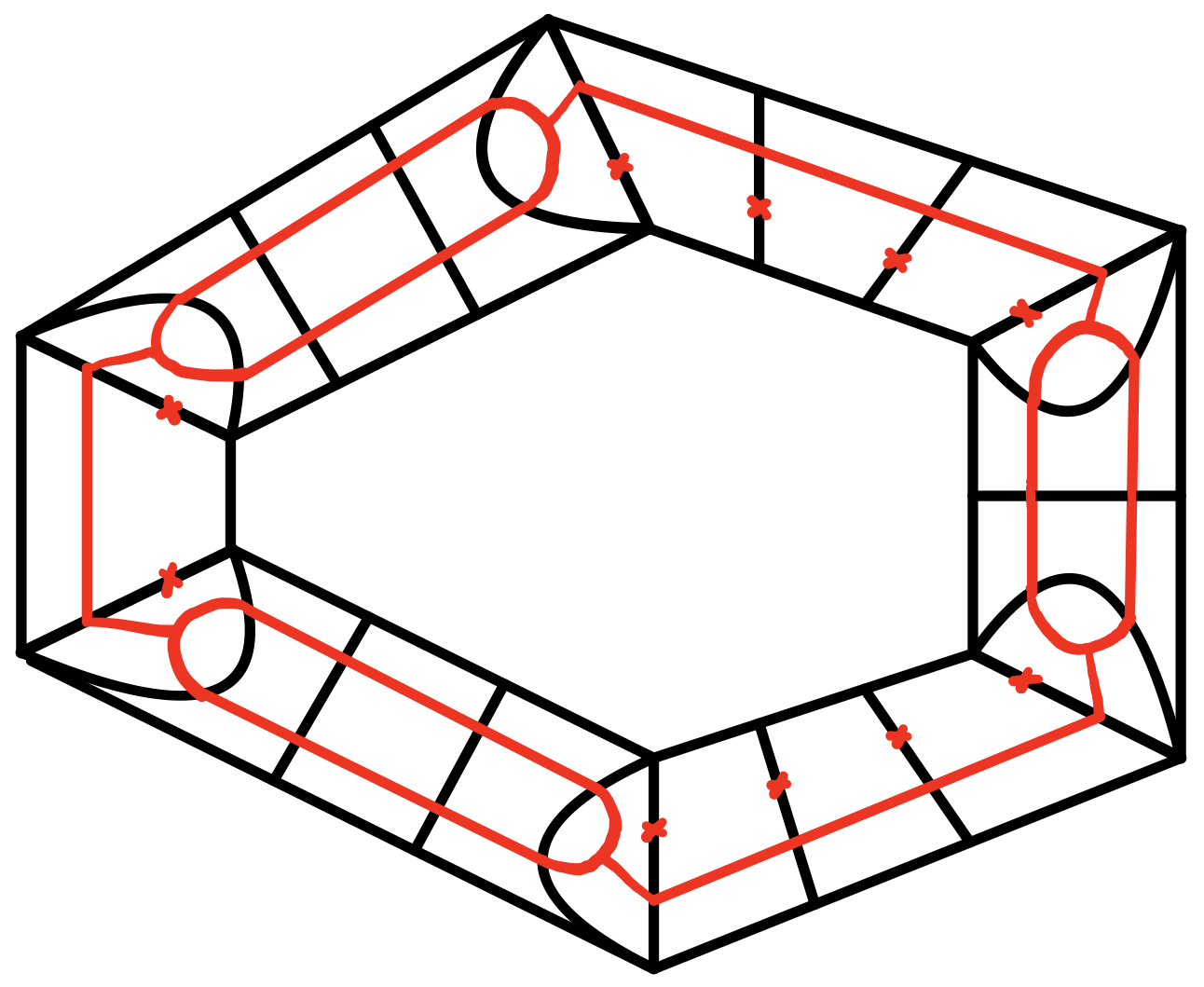
Figure 11. Kulikov models for the $\bar{g}=1$ case

Next are the pairs corresponding to the nonsingular lattice points on the equator. These are of types E1 or E2 of Lemma 8.5 respectively for the sides of ${\widehat{Y}}$ with $E_{i}^{2}=-1$ and $E_{i}^{2}=-4$.

Finally, we need to determine the cbec, together with the involution, of an $I_{1}$ singularity at a vertex of the polytope $P$. From either Fig. 6 or 10 we see that the minimal pseudofan for this singularity consists of two rays $v_{1}=(-2,1)$ on the side with $E_{1}^{2}=-1$, $v_{2}=(1,0)$ on the side with $E_{2}^{2}=-4$, and the monodromy ray $v_{\rm mon}=(0,-1)$. The balancing condition for these vectors is $v_{1}+2v_{2}=-v_{\rm mon}$. This is the pseudofan of $({\mathbb{P}}^{2},D_{1}+D_{2})$ with $D_{1}$ a line (so $D_{1}^{2}=1$), $D_{2}$ a conic (so $D_{2}^{2}=4$), and an involution whose fixed locus is a line $R$ and an isolated point. The balancing condition [AET19, Sec. 2E] reads $\sum_{i=1}^{2}(R\cdot D_{i})v_{i}\in{\mathbb{Z}}v_{\rm mon}$.

Therefore, $B$ is the $\operatorname{IAS}^{2}$ given by Construction 6.15 for the surfaces $X_{0}$ glued from $2k$ pairs in the cbec of $({\mathbb{P}}^{2},D_{1}+D_{2})$, $\bar{k}$ chains of lengths $\ell_{i}=L\cdot E_{i}$ of type E1 for odd $i$, $\bar{k}$ chains of lengths $\ell_{i}=L\cdot E_{i}$ of type E2 for even $i$, $12-\bar{k}$ pairs of almost toric surfaces with a single blowup, and the rest toric pairs. The triangulation ${\mathcal{T}}$ specifies the combinatorial type of each pair precisely.

This surface can be read of directly from the Coxeter diagram for the lattice ${\overline{T}}$ given in Figs. 3, 4. The most relevant part is the cycle of $2\bar{k}$ white vertices, alternating between double circled and single circled. Each edge on this cycle corresponds to a ${\mathbb{P}}^{2}$. A single circled vertex, with odd $i$ corresponds to a line, and a double circled vertex, with even $i$ corresponds to a conic on ${\mathbb{P}}^{2}$.

Each integral vector $\lambda\in{\mathfrak{C}}_{\rm r}$ defines the nonnegative integers $\ell_{i}=\lambda\cdot\alpha_{i}$. The numbers $\ell_{i}$ for these $2\bar{k}$ simple roots $\alpha_{i}$ on the $2\bar{k}$-cycle specify the lengths of chains as above. In addition, the other $\ell_{i}$ define the locations of the nontoric surfaces in the hemispheres. On the mirror side, if ${\widehat{Y}}\to{\overline{Y}}$ is a toric model with exceptional curves $E_{i}$, $i>2\bar{k}$, then $E_{i}$ correspond to some of the vertices in the Coxeter diagram and the lattice distance of a singularity from the equator is determined in terms of $\ell_{i}=L\cdot C_{i}$. We give a cartoon picture for the equator of $X_{0}$ in Fig. 11, with the fixed locus shown in red. The divisorial part $R_{0}$ of ${\rm Fix}(\iota_{0})$ is a degeneration of genus $3$ curves ${\rm Fix}(\iota_{t})$.

A detailed example of this construction was given in [AET19] for ${\overline{T}}=(19,1,1)$. In that case, there are $18$ $I_{1}$ singularities on the equator, and $3$ pairs of $I_{1}$ singularities in the hemispheres. The lengths $\ell_{0},\dotsc,\ell_{17}$ give the lengths of the chains of toric surfaces on the equator. On the mirror side, the morphism to the toric model ${\widehat{Y}}\to{\overline{Y}}$ consists of three disjoint blowups, and the distances of the nontoric surfaces $V_{j}$ from the equator are $L\cdot E_{i}$ for $i=18,19,20$.

Each of the lattices ${\overline{T}}$ on the $\bar{g}=1$ line is the target of a unique mirror move $S\to T\leadsto{\overline{T}}$ as in Definition 5.6, which is simple. So $S\subset L_{\rm IAS}$ is saturated and the set of symmetric periods is the torus ${\mathbb{T}}_{\Lambda/S}$ and the family of Type III surfaces contains the standard surface corresponding to the period $\psi=1$.

8D. Models for ${\overline{T}}$ with $\bar{g}\geq 2$, excluding $(10,8,0)$

We use the reduction from the $\bar{g}=1$ case given in Section 4F. The lattice

$${\overline{T}}={\widehat{S}}=(10+\bar{k}-(\bar{g}-1),10-\bar{k}-(\bar{g}-1),\bar{\delta})$$

is obtained from the lattice ${\overline{T}}^{\prime}={\widehat{S}}^{\prime}=(10+\bar{k},10-\bar{k},1)$ by a chain of $\bar{g}-1$ Heegner $(-1,-1)$ moves. The set of possible monodromy invariants $\lambda\in{\overline{T}}$ lie in the fundamental chamber for ${\overline{T}}$ which is a face of the fundamental chamber for ${\overline{T}}^{\prime}$, obtained by setting some of the lengths $\ell_{i}$ with $i>2\bar{k}$ to zero.

By Theorem 7.4 the $\operatorname{IAS}^{2}$ for ${\overline{T}}$ is obtained from the $\operatorname{IAS}^{2}$ for ${\overline{T}}^{\prime}$ by descending $(\bar{g}-1)$ pairs of $I_{1}$ singularities in the interiors of the hemispheres symmetrically to the equator, to a side of type E1 of Lemma 8.5 with odd equatorial behavior, to get an $I_{2(\bar{g}-1)}$ singularity with monodromy rays parallel to the equator.

What remains to see is an involution on an actual surface $X_{0}$ and specifically the surfaces $V_{i}$ with involution on the equator. To describe them we introduce two moves, illustrated in Fig. 12.

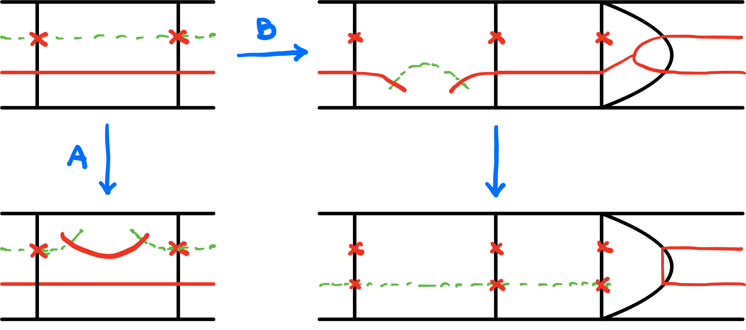
Figure 12. A- and B-moves

A-move: Let $V^{\prime}\to{\mathbb{P}}^{1}$ be a toric surface of type E1 of Lemma 8.5. The A-move is blowing up one of the fixed points on a section, say $s_{1}$ twice. In the corresponding fiber of $V\to{\mathbb{P}}^{1}$ this creates the fiber $E_{1}+2E_{2}+E_{3}$ with $E_{1}^{2}=E_{3}^{2}=-1$ and $E_{2}^{2}=-2$, the the interior $(-2)$-curve $E_{2}$ is fixed by the induced involution of $V$.

Let $(g,k)$ be the invariants of the K3 surfaces in the $S^{\prime}$ family, so that ${\overline{T}}^{\prime}$ was reached by the simple mirror move $S^{\prime}\to{\overline{T}}$. Then the Type III surface we obtained belongs to the $S$-family with the invariants $(g,k+1)$.

The point we have blown up twice in the toric model ${\overline{V}}^{\prime}$ of $V^{\prime}$ corresponds to $-1$ with respect to the origin of the blown up side. Therefore, we can for example take $X_{0}$ of this type to be the standard surface, with $\psi=1$. In particular, the A-move keeps a simple mirror move $S\to{\widehat{S}}$ simple, in the sense that $S$ changes by a $(+1,-1)$ Heegner move, while ${\widehat{S}}$ changes by a $(-1,-1)$ Heegner move.

B-move: For the B-move we instead blow up twice the other fixed point, the one that lies on a fiber fixed by the involution pointwise. On the surface $\operatorname{Bl}_{2}V$ the fixed locus of the involution consists of two $(-1)$-curves $E_{1}$, $E_{3}$ in the fiber $E_{1}+2E_{2}+E_{3}$. The divisor $V^{\iota}$ fixed by the induced involution is not nef since it contains $E_{1}$ and $E_{3}$ and not $E_{2}$.

We flop $E_{1}$ to a neighboring surface $V_{1}$ by the M1 modification. In $V_{1}$ this creates a fiber $E_{1}^{\prime}+E_{2}^{\prime}$ with $E^{\prime}_{1}{}^{2}=E^{\prime}_{2}{}^{2}=-1$, where $E^{\prime}_{1}$ is not in $V_{1}^{\iota}$ and $E^{\prime}_{2}$ is. The ramification divisor is not nef again. We proceed by flopping in $E^{\prime}_{2}$ etc, until we reach a component in the cbec of $({\mathbb{P}}^{2},D_{1}+D_{2})$ corresponding to the $I_{1}$ singularity of the $\operatorname{IAS}^{2}$. This is where the sequence of flops stops, making $({\mathbb{P}}^{2},D_{1}+D_{2})$ with $D_{1}^{2}=1$, $D_{2}^{2}=4$ into $({\mathbb{F}}_{1},D_{1}+D_{2})$ with $D_{1}^{2}=0$, $D_{2}^{2}=4$ and the ramification into a fiber of ${\mathbb{F}}_{1}\to{\mathbb{P}}^{1}$.

We do the same with the other $(-1)$-curve $E_{3}$ on $V$, flopping it all the way to the surface in the cbec of $({\mathbb{P}}^{2},D_{1}+D_{2})$ on the equator in the other direction. The end result is that the entire chain of surfaces between the two $({\mathbb{P}}^{2},D_{1}+D_{2})$-components, which in $X^{\prime}_{0}$ was a chain of toric surfaces of equatorial type E1 is now a chain of toric surfaces of equatorial type E0, with no divisorial part in the fixed locus.

If $(g,k)$ are the invariants of the K3 surfaces in the $S^{\prime}$ family then the Type III surface $X_{0}$ obtained by the B-move has invariants $(g-1,k)$ and thus must be the result of a non-simple mirror move.

Now repeat this procedure $(\bar{g}-1)$ times doing either the A-move every time, or $(\bar{g}-2)$-times the A-move and once the B-move. Let $X_{0}$ be either of the surfaces obtained this way. There is an entire $19$-dimensional family $\operatorname{Hom}(\Lambda,{\mathbb{C}}^{*})$ of $d$-semistable surfaces $X_{0}(\psi)$ of the same deformation type.

As in Theorem 8.3, the subset of anti-symmetric periods is a union of torus translates of ${\mathbb{T}}_{\Lambda/\Lambda^{+}}:={\rm Hom}(\Lambda/\Lambda^{+},{\mathbb{C}}^{*})$. As before, $\Lambda=\lambda^{\perp}$ in $L_{\rm IAS}$, ${\overline{T}}=L_{\rm IAS}^{-}$, and $\Lambda^{+}=L_{\rm IAS}^{+}=({\overline{T}})^{\perp}=S^{\rm sat}$ in $L_{\rm IAS}$. The coset of ${\mathbb{T}}_{\Lambda/\Lambda^{+}}$ containing the standard surface is of the A…A type, and all other involution anti-invariant cosets of ${\mathbb{T}}_{\Lambda/\Lambda^{+}}$ are of the A…AB type.

8E. Monodromy invariants for ${\overline{T}}=(10,10,0)$

In this case, the source of the mirror move must be $S=(10,10,0)$, so ${\overline{T}}$ corresponds to the self-mirror cusp of Enriques K3 moduli.

By Theorem 7.4 and Lemma 7.1, the $\operatorname{IAS}^{2}$ $B=P\cup P^{\rm opp}$ in this case is obtained from the $\operatorname{IAS}^{2}$ $B^{\prime}=P\cup P^{\rm opp}$ of the $(10,10,1)$ case by gluing $P^{\rm opp}$ to $P$ by twisting halfway along the circular boundary. This is possible, so long as the affine length of the equator is even, which can always be achieved by replacing $\lambda$ by $2\lambda$. So the Type III surface is obtained from a Type III surface of the $(10,10,1)$ case by this rotation. The involution $\iota_{0}$ on $X_{0}$ is base point free.

$(10,10,0)$ is the only case when the fundamental chambers ${\mathfrak{C}}_{2}$ and ${\mathfrak{C}}_{\rm r}$ are not the nef cones of quotient surfaces ${\widehat{Y}}$. Indeed, for a general Enriques surface ${\widehat{Y}}$ the nef cone is the round cone $\overline{{\mathcal{C}}}$. On the other hand, in the $\operatorname{IAS}^{2}$ $B$, we used the Symington polytope $P$ from the Halphen $(10,10,1)$ case, which certainly has polyhedral walls, and so is not the entire round cone.

On the other hand, ${\mathfrak{C}}_{\rm r}(10,10,0)$ is a subset of ${\mathfrak{C}}_{\rm r}(10,10,1)$. Indeed, the Coxeter diagrams for both lattices are given in Fig. 3 and they are nearly identical. Denote the simple root vectors in $E_{8}(2)$ by $\alpha_{1},\dotsc,\alpha_{8}$, so that $\alpha_{i}^{2}=-4$ and $\alpha_{i}\cdot\alpha_{j}\in\{0,2\}$ for $i\neq j$. Let $U=\langle e,f\rangle$ with $e^{2}=f^{2}=0$, $e\cdot f=1$. One has $(10,10,0)=E_{8}(2)\oplus U(2)$ and $(10,10,1)=E_{8}(2)\oplus I_{1,1}(2)$, where $U(2)=\langle 2e,f\rangle$ and $I_{1,1}=\langle 2e,e+f\rangle$ are two different index $2$ sublattices of $U$.

Then the first $9$ vectors of the two Coxeter diagrams are exactly the same: $\alpha_{1},\dotsc,\alpha_{8},\alpha_{9}=2e-\alpha_{0}$, where $-\alpha_{0}$ is the longest root of $E_{8}$. It is only the last, $10$th roots that are different. For $(10,10,0)$ it is $\alpha_{10}=-2e+f$, and for $(10,10,1)$ it is $\alpha^{\prime}_{10}=-e+f$. Thus, $\alpha^{\prime}_{10}=\alpha_{10}+e$. Since $e$ is a positive linear combination of $\alpha_{1},\dotsc,\alpha_{9}$, if $\lambda$ is a vector in ${\mathfrak{C}}_{\rm r}(10,10,0)$, i.e. a vector satisfying $\lambda\cdot\alpha_{i}\geq 0$ for $i=1,\dotsc,10$ then one moreover has $\lambda\cdot\alpha^{\prime}_{10}\geq 0$.

So for any $\lambda\in{\mathfrak{C}}_{\rm r}(10,10,0)\subset{\mathfrak{C}}_{\rm r}(10,10,1)$ we interpret $\lambda$ as a vector defining the Symington polytope for $(10,10,1)$ by the previous construction, and take $B$ to be $P\cup P^{\rm opp}$ glued with a half-circle rotation in the equator.

8F. Models for ${\overline{T}}=(10,8,0)$, $(10,10,0)$, $(10,10,1)$

There are five mirror moves $S\leadsto{\overline{T}}$ for which the integral affine structure $B=P\cup P^{\rm opp}$ has a circular equator with no singularities on it. They are:

(6) $$\begin{aligned} &(10,10,0)\to(10,10,0),&&(10,10,1)\to(10,10,1),\\ &(10,8,0)\to(10,8,0),&&(10,10,0)\Rightarrow(10,8,0),&&(10,10,1)\Rightarrow(10,8,0).\end{aligned}$$

In particular, the lattice ${\overline{T}}=(10,8,0)$ is the target of three mirror moves. Respectively, there are three families of Type III surfaces with anti-symmetric periods. All of them share the same $\operatorname{IAS}^{2}$ $B=P\cup P^{\rm opp}$, glued from two copies of a Symington polytope $P$ for the anticanonical pair $({\widehat{Y}},{\widehat{D}})$ with ${\widehat{Y}}=Bl_{p_{1},\dots,p_{9}}{\mathbb{P}}^{2}$ and ${\widehat{D}}$ the strict transform of a cubic through the nine points $p_{i}$. The gluing as in Section 8B is with the even equatorial behavior. The only difference is in the periods.

For the $(10,10,1)\to(10,10,1)$ mirror move, the target $\operatorname{IAS}^{2}$ determined by ${\overline{T}}$ is $P\cup P^{\rm opp}$ with $P$ as in the previous paragraph, but with the odd equatorial behavior.

The $(10,10,0)\to(10,10,0)$ mirror move is the only one for which the target $\operatorname{IAS}^{2}$ satisfy $B/\iota\simeq{\mathbb{R}}{\mathbb{P}}^{2}$. There is no well-defined equatorial edge behavior since the edge is not fixed, and the sphere $B$ is built from Symington polytopes for $({\widehat{Y}},{\widehat{D}})$ with a half-twist, as in Section 8E.

The shape of the equator, and the fixed locus of $\iota_{0}$ inside it, is depicted in Figure 13, in the respective positions of the mirror moves in Equation 6. In all cases, the equatorial behavior of $R_{0}$ depicted is uniquely determined by the fact that the divisorial part of $R_{0}$ must be the flat limit of $R_{t}$.

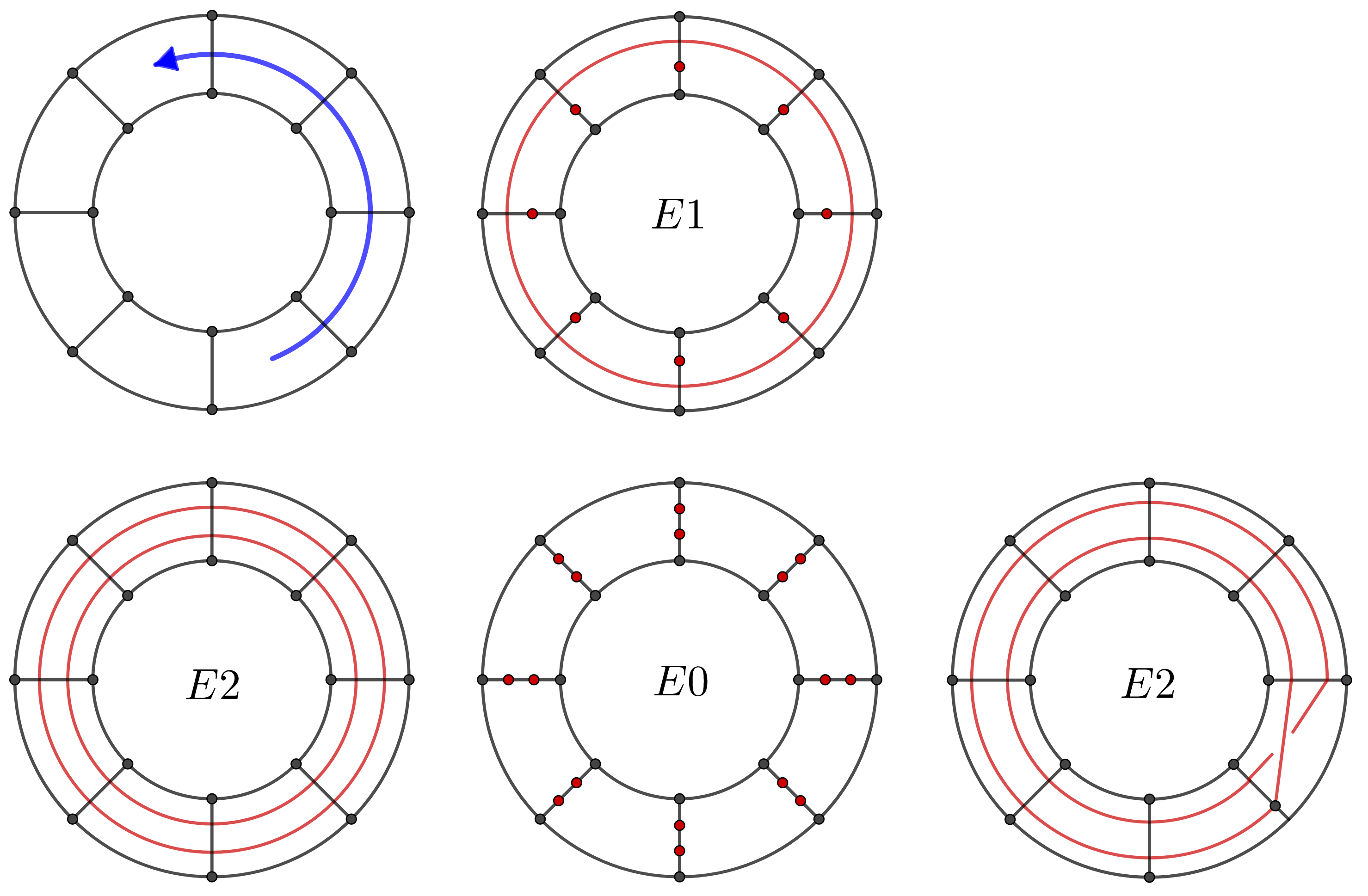
Figure 13. The fixed loci in circular equators, shown in red, and the corresponding edge behavior.

8G. Colliding singularities and non-generic type III models

In the previous sections, we defined Kulikov models for the generic $\lambda$. With the exception of Section 8D, the $\operatorname{IAS}^{2}$ had $24$ distinct $I_{1}$ singularities: $2\bar{k}$ of them lie on the equator, and $12-\bar{k}$ in the interior of each of the hemispheres $P$, $P^{\rm opp}$ in pairs, so that the whole collection is preserved by the involution $P\leftrightarrow P^{\rm opp}$.

For a non-generic $\lambda$ and for the lattices with $\bar{g}\geq 2$, some of these singularities collide to form integral-affine singularities of higher charge.

Each of the $I_{1}$ singularities on the equator corresponds to a surface in the cbec of $({\mathbb{P}}^{2},D_{1}+D_{2})$ and the ramification divisor is a line $L$ of volume $L^{2}=1$. Also, after a B-move, the M1 modifications convert each end $({\mathbb{P}}^{2},D_{1}+D_{2})$ into $({\mathbb{F}}_{1},D_{1}+D_{2})$ with the ramification divisor a fiber, of volume $L^{2}=0$.

On the other hand, the off-equator $I_{1}$ singularities correspond to surfaces with an empty ramification divisor, of volume $0$. When singularities collide, the volumes add. The anticanonical pairs of volume $0$ get contracted on the stable models, which are described in Section 9B. This leads to three types of collisions:

(1) Collisions in the interiors of the hemispheres $P$, $P^{\rm opp}$. These are completely irrelevant and can be avoided by nodal slides, replacing them by isolated $I_{1}$. The corresponding anticanonical pairs $(V_{i},D_{i})$ are disjoint from the $C_{g}$ component of the ramification divisor $R$, so on the stable model $V_{i}$ will be contracted to points.

(2) Collisions obtained by descending pairs of $I_{1}$ singularities to the equator. These are only partly relevant: without further collisions, the curve $C_{g}$ has numerical dimension $1$ or $0$ on the corresponding pair $(V_{i},D_{i})$. So on the stable model, $V_{i}$ is contracted to ${\mathbb{P}}^{1}$ or a point and the collision is not detected by the stable model.

(3) The singularities obtained by colliding some of the $2\bar{k}$ $I_{1}$ singularities on the equator, between themselves, or with some of the pairs of $I_{1}$ singularities from case (2). These are truly relevant. Each isolated $I_{1}$ singularity on the equator corresponds to a pair $(V_{i},D_{i})$ in the cbec of $({\mathbb{P}}^{2},D_{1}+D_{2})$ with a line and a conic, and the curve $C_{g}$ restricts to this ${\mathbb{P}}^{2}$ as a line. On the stable model, this $V_{i}$ will not be contracted, mapping to a surface whose normalization is ${\mathbb{P}}^{2}$. Further collisions lead to more complicated nontoric anticanonical pairs $(V_{i},D_{i})$ with big and nef $C_{g}$, and to more complicated irreducible components of the stable model.

Below, we work with the chamber ${\mathfrak{C}}_{2}$ and its Coxeter diagram $\Gamma_{2}$. The translation between ${\mathfrak{C}}_{2}$ and ${\mathfrak{C}}_{\rm r}$ and the elliptic subgraphs of $\Gamma_{2}$ and $\Gamma_{\rm r}$ is given by Eq. (3) and Fig. 2.

Definition 8.6.

For any $\lambda\in{\mathfrak{C}}_{2}$ define the subdiagram $\Gamma_{2}(\lambda)\subset\Gamma_{2}$ with the vertices

$$V_{2}(\lambda)=\{i\mid\ell_{i}=0\},\quad\text{where }\ell_{i}=\lambda\cdot\alpha_{i}\text{ for simple roots }\alpha_{i}.$$

Recall that $\ell_{i}\geq 0$ for any $\lambda\in{\mathfrak{C}}_{2}$. $\Gamma(\lambda)$ specifies the face of ${\mathfrak{C}}_{2}$ to which $\lambda$ belongs.

Further, by Section 4F, for a lattice ${\overline{T}}$ of genus $\bar{g}$ the chamber ${\mathfrak{C}}_{2}({\overline{T}})$ is a face of the chamber ${\mathfrak{C}}_{2}({\overline{T}}_{1})$ for the “parent” lattice ${\overline{T}}_{1}={\overline{T}}\oplus A_{1}^{\bar{g}-1}$. Let $\Gamma_{2}^{\rm par}(\lambda)\subset\Gamma_{2}({\overline{T}}_{1})$ be the diagram of $\lambda$ considered as a vector in ${\overline{T}}_{1}$. With notations of Corollary 4.13 one has $\Gamma_{2}^{\rm par}(\lambda)=\Gamma(\lambda)+A_{1}^{\bar{g}-1}$, see Lemma 4.16.

By Eq. (2) in Section 3, if $\lambda^{2}>0$ then $\Gamma_{2}^{\rm par}(\lambda)$ is elliptic, i.e. a disjoint union of $ADE$ diagrams. As in Section 6G, these $ADE$ diagrams correspond to collections of visible curves connecting the $I_{1}$ singularities. We illustrate this in Fig. 14 showing a collision of type (2) that gives an $I_{2}$ of charge $Q=2$ and a collision of type (3) that gives $D_{5}$ of charge $Q=8$.

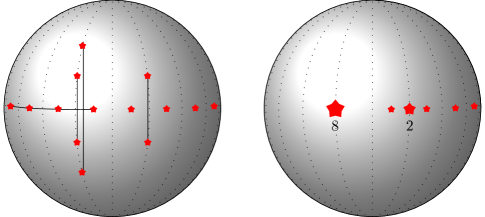
Figure 14. Colliding $I_{1}$ singularities: $D_{5}$ (charge $=8$, volume $=4$) and $A_{1}$ (charge $=2$, volume $=0$)

The visible curves $(\gamma_{i},\alpha_{i})$ connecting the pairs of $I_{1}$ singularities with the same monodromy directions are in a bijection with some of the simple roots $\alpha_{i}$ of $\Gamma_{2}^{\rm par}$. The corresponding lengths $\ell_{i}=\lambda\cdot\alpha_{i}$ measure the lattice distances between these $I_{1}$ singularities. A collision occurs when all of these distances become zero.

For each singularity of type (3) the divisor $C_{g}$ on the corresponding anticanonical pair $(V,D)$ is big and nef, so $K_{V}+D+\epsilon C_{g}$ is big and nef. Its canonical model $({\overline{V}},{\overline{D}}+\epsilon{\overline{C}}_{g})$ is one of the $ADE$ stable involution pairs which were completely classified in [AT21, Table 2]. The cbec of $(V,D)$ is the cbec of the minimal resolution of singularities of $({\overline{V}},{\overline{D}})$.

[AT21] devised an elaborate system for denoting the $ADE$ surfaces using decorated Dynkin symbols. For example the $D_{5}$ singularity of Fig. 14 corresponds to $\kern-2.0pt\phantom{.}^{\prime}\kern-2.0ptD_{5}^{-}$ of [AT21, Table $1$]. Perhaps the easiest way to understand them is to look at the $ADE$ subgraphs of the Coxeter diagrams in Figs. 3, 4, while remembering the conversion rules of Eq. (3) and Fig. 2. Such a subgraph $G$ contains more information that just its $ADE$ type. For example, an $A_{n}$ subgraph can sit in $\Gamma_{2}$ in many different ways: it may lie entirely in the equatorial $2\bar{k}$-cycle, or one or two of its vertices may venture off-equator. It may begin at a single-circled or a double-circled white vertex. All of these possibilities correspond to different cbecs of anticanonical pairs with an involution. But the decorated $ADE$ symbols specify them uniquely.

The most useful way to think of an $ADE$ subgraph $G\subset\Gamma_{2}$ is as a chain in the equatorial $2\bar{k}$ cycle, plus some off-equator vertices each attached to an even-numbered equatorial, double-circled white vertex $\alpha_{i}$. For a given $\alpha_{i}$, the off-equator vertices $\beta_{j}$ connected to it are disjoint from each other, cf. Fig. 2.

With the singularities of $B=\Gamma(X_{0})$ modeled by the cbecs of the corresponding $ADE$ surfaces of [AT21], the proof of Theorem 8.3 goes through, essentially unchanged.

8H. Type II models

Type II degenerations correspond to monodromy vectors $\lambda\in{\mathfrak{C}}_{2}$ with $\lambda^{2}=0$. On the mirror side, the line bundle $L\in{\widehat{S}}$ is nef but not big, $L^{2}=0$. Since the lattice area of $\operatorname{IAS}^{2}$ is $\lambda^{2}=L^{2}$, the sphere degenerates to an interval, the dual complex of a Type II Kulikov model. The limit of an $\operatorname{IAS}^{2}$ $B=P\cup P^{\rm opp}$ with an involution itself has an involution, so the interval is either vertical, going from one pole of the sphere to another, or horizontal.

The subgraph $\Gamma_{2}(\lambda)$ in this case is parabolic, a disjoint union of finitely many ${\widetilde{A}}_{n}$, ${\widetilde{D}}_{n}$, ${\widetilde{E}}_{n}$ extended Dynkin diagrams. Just as in the previous section, the collisions are of types (1) irrelevant, (2) partly relevant but not changing the stable model, and (3) those that include some vertices on the $2\bar{k}$-cycle, which do affect the stable models. The stable models for $(V_{i},D_{i},\epsilon C_{g})$ in this case are the ${\widetilde{A}}{\widetilde{D}}{\widetilde{E}}$ surfaces classified in [AT21] and $(V_{i},D_{i})$ are their resolutions to nonsingular pairs.

9. Compact moduli

We now restrict ourselves to the moduli spaces $F_{S}$ for the $50$ lattices $S$ of Fig. 1 for which $g\geq 2$, excluding $(10,8,0)$. In these cases the ramification divisor $R=X^{\iota}$ has a unique component $C_{g}$ of genus $g\geq 2$. If $X\to{\overline{X}}$ is the contraction given by a linear system $|mC_{g}|$ then the image ${\overline{C}}_{g}$ of $C_{g}$ is an ample Cartier divisor on ${\overline{X}}$ and the pair $({\overline{X}},\epsilon{\overline{C}}_{g})$ is a stable KSBA pair for $0<\epsilon\ll 1$, so one has the KSBA compactification as in Section 2E. Recall that we denoted the main component ${\overline{F}}_{S}$ and its normalization was the semitoric compactification ${\overline{F}}^{\mathfrak{F}}=({\overline{F}}_{S})^{\nu}$ by Proposition 8.1.

The goal of this section is to prove the Main Theorem 9.10. The proof is given in Section 9C. We begin by defining the semifans ${\mathfrak{F}}_{I}={\mathfrak{F}}_{\rm ram}({\overline{T}})$ forming ${\mathfrak{F}}$ as one ranges over the $0$-cusps $I=e^{\perp}/e$. Then, we discuss stable models.

9A. The ramification semifan

We use the same notations as in Section 3A. Let $H={\overline{T}}=e^{\perp}_{T}/e$ be the hyperbolic lattice corresponding to a $0$-cusp of $F_{S}$. Let $\Gamma$ be its Coxeter diagram.

Recall that we defined the Coxeter semifan in Section 3B. We now define a generalized Coxeter semifan by the “Wythoff’s construction” of [Cox35]. We refer to [AET19, Sec. 10C] for details.

Divide the vertex set $V(\Gamma)$ of the Coxeter diagram into two sets $V_{\rm rel}\sqcup V_{\rm irr}$ of relevant and irrelevant roots. (It is important to understand that the “irrelevant” vertices are irrelevant only when in isolation. They become relevant if they are connected to the relevant ones.)

Definition 9.1.

Modulo $W$, the fan ${\mathfrak{F}}_{\rm gen}$ has a unique maximal dimensional cone

$${\mathfrak{C}}_{\rm gen}=\cup_{w\in W_{\rm irr}}w.{\mathfrak{C}},\quad\text{where }W_{\rm irr}=\langle w_{i}\mid i\in V_{\rm irr}\rangle.$$

All the other cones in ${\mathfrak{F}}_{\rm gen}$ are the faces of ${\mathfrak{C}}$ and their $W$-translates.

Example 9.2.

Consider the Coxeter fan for $W(A_{2})=S_{3}$ in ${\mathbb{R}}^{2}$, consisting of $6$ two-dimensional cones and their faces. If we take for $V_{\rm irr}$ one of the vertices of the $A_{2}$ diagram then ${\mathfrak{F}}_{\rm gen}$ will be a fan with $3$ two-dimensional cones and it is not a reflection fan.

${\mathfrak{F}}_{\rm gen}$ has fewer cones than ${\mathfrak{F}}$ in the following sense:

Definition 9.3.

Let $V^{\prime}\subset V(\Gamma)$ be a subset of vertices and $\Gamma^{\prime}\subset\Gamma$ the induced subdiagram which is either elliptic or parabolic. We divide $V^{\prime}$ into the relevant and irrelevant parts $\operatorname{rel}(V^{\prime})\sqcup\operatorname{irr}(V^{\prime})$ as follows: the vertices of the connected components of $\Gamma^{\prime}$ that consist entirely of irrelevant vertices form $\operatorname{irr}(V^{\prime})$, and the rest is $\operatorname{rel}(V^{\prime})$. We say that $\operatorname{rel}(V^{\prime})$ is the relevant content of $V^{\prime}$.

Then the cone $F^{\prime}$ of ${\mathfrak{F}}_{\rm gen}$ defined by $V^{\prime}$ is the same as the one defined by its relevant content, and $F\cap{\mathfrak{C}}$ is the cone $F(\operatorname{rel}(V^{\prime}))$ of ${\mathfrak{F}}$. In particular, if $\operatorname{rel}(V^{\prime})=\emptyset$ then $V^{\prime}$ does not define any cone in ${\mathfrak{F}}_{\rm gen}$ at all.

Remark 9.4.

Let $W=W_{\rm r}$. If $V_{\rm irr}={\mathbb{B}}$ is a subset of $V_{4}$ as in Definition 3.2 then by Lemma 3.3 ${\mathfrak{F}}_{\rm gen}$ is simply the Coxeter semifan for the Weyl group $W_{\rm nor}({\mathbb{B}}^{c})$. But in our case the set $V_{\rm irr}$ is bigger than $V_{4}$, and ${\mathfrak{F}}_{\rm gen}$ is not a Coxeter semifan for any Weyl group.

Definition 9.5.

Let ${\overline{T}}_{1}=(10+\bar{k},10-\bar{k},\bar{\delta})$, $1\leq\bar{k}\leq 9$ be a lattice on the $\bar{g}=1$ line and $\Gamma({\overline{T}}_{1})$ be its Coxeter diagram as in Sections 3D, 3E. We declare the only relevant vertices $V_{\rm rel}$ to be the $2\bar{k}$ vertices on the $I_{2\bar{k}}$ cycle, and all the other vertices to be irrelevant. In particular, all the black vertices are irrelevant.

Any other lattice ${\overline{T}}$ appearing as the target of a mirror move $S\leadsto{\overline{T}}$ for $S$ with $g\geq 2$ is of the form ${\overline{T}}_{\bar{g}}=(10+\bar{k}-(\bar{g}-1),10-\bar{k}-(\bar{g}-1),\bar{\delta})$. By Corollary 4.13, it can be reached from ${\overline{T}}_{1}=(10+\bar{k},10-\bar{k},1)$ by a chain of $\bar{g}-1$ standard operations described in Lemma 4.15, and the set of vertices of $\Gamma({\overline{T}}_{\bar{g}})$ is a subset of the vertices of $\Gamma({\overline{T}}_{1})$ We declare the vertices of $\Gamma({\overline{T}}_{\bar{g}})$ to be relevant if they were also relevant in $\Gamma({\overline{T}}_{1})$. For $\bar{g}\geq 2$ there are $2\bar{k}-1$ of them.

We define the semifan ${\mathfrak{F}}_{\rm ram}({\overline{T}})$ to be the generalized Coxeter fan for this set $V_{\rm irr}$ of relevant vertices. It is a coarsening of the reflection fan ${\mathfrak{F}}_{2}$ for the $(-2)$-roots: Walls of ${\mathfrak{F}}_{2}$ get erased exactly when they are the perpendicular to an entirely irrelevant diagram.

9B. Stable models

Let $X_{0}$ be one of the Type III surfaces with an involution $\iota$ defined in Section 8A, $R$ the divisorial part of the fixed locus $X^{\iota}$, and $C_{g}$ the connected component of $R$ that has arithmetic genus $g\geq 2$. In each case, we constructed a family $X_{0}$ of such surfaces with an involution, parameterized by a translate of a torus. After any necessary M1 modifications resulting from a B-move, see Section 8D, the limit of $C_{g}$ is a big and nef divisor, and a large multiple $|mC_{g}|$ defines a contraction $f\colon X_{0}\to{\overline{X}}_{0}$. Denote by ${\overline{C}}_{g}$ the image of $C_{g}$, it is a Cartier divisor. The pair $({\overline{X}}_{0},\epsilon{\overline{C}}_{g})$ is a KSBA stable pair, see Section 2E.

Lemma 9.6.

Let $X_{0}=\cup V_{i}$ with $V_{i}$ corresponding to the lattice points of $B=P\cup P^{\rm opp}$. Assume $\bar{g}=1$. Then under the morphism $f\colon X_{0}\to{\overline{X}}_{0}$

1. if $i$ is in the interior of $P$ or $P^{\rm opp}$ then $V_{i}$ is contracted to a point,

2. if $i$ is on the equator but not at a vertex of $P$ then $V_{i}$ is contracted to ${\mathbb{P}}^{1}$,

3. if $i$ is a vertex of $P$ on the equator then $V_{i}\to{\overline{V}}_{i}$ is birational.

Proof.

Indeed, by construction, these are the irreducible components of $X_{0}$ on which $C_{g}$ has numerical dimension $0$, $1$, $2$, compare the description of the pairs $(V_{i},D_{i})$ of types (1), (2), (3) in Section 8G. ∎

Recall that a lattice ${\overline{T}}_{\bar{g}}=(10+\bar{k}-(\bar{g}-1),10-\bar{k}-(\bar{g}-1),\bar{\delta})$ of genus $\bar{g}>1$ is reached from ${\overline{T}}_{1}=(10+\bar{k},10-\bar{k},1)$ by a chain of $\bar{g}-1$ standard operations described in Lemma 4.15. By the construction of Section 8D, if the mirror move $S\to{\overline{T}}$ is odd then the Kulikov surface for ${\overline{T}}_{\bar{g}}$ is obtained from that of ${\overline{T}}_{1}$ by a sequence of moves A…AA, and if $S\Rightarrow{\overline{T}}$ is even then it is by a sequence of moves A…AB. In either case, if $\bar{g}\geq 2$ then the $I_{2\bar{k}}$-cycle on the equator is broken and becomes a chain of length $2\bar{k}-1$.

Definition 9.7.

Let $(V,D=\sum D_{j})$ be an anticanonical pair and $L$ be a big and nef divisor on $V$. We say that an irreducible component $D_{j}$ of $D$ is a short side if $LD_{j}=1$, a long side if $L\cdot D_{j}=2$, and a zero side if $L\cdot D_{j}=0$. If $f\colon V\to{\overline{V}}$ is the contraction defined by $L$ and $L=f^{*}{\overline{L}}$, then we say that the images ${\overline{D}}_{j}$ of $D_{j}$ are short or long sides of ${\overline{V}}$ if ${\overline{L}}\cdot{\overline{D}}_{j}=1$ or $2$ respectively.

Definition 9.8.

We define two types of stable models ${\overline{X}}_{0}=\cup_{i}({\overline{V}}_{i},{\overline{D}}_{i},\epsilon{\overline{C}}_{g,i})$, illustrated in Fig. 15.

(1) Pumpkin. Each surface ${\overline{V}}_{i}$ has two sides ${\overline{D}}_{i}={\overline{D}}_{i,}{}_{\rm left}+{\overline{D}}_{i,}{}_{\rm right}$, they are glued in a circle, all of $D_{i}$ meeting at the north and south poles.

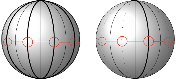
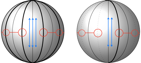
Figure 15. Pumpkin and smashed pumpkin type stable models

(2) Smashed pumpkin. Starting with a surface of the pumpkin type, one short side is contracted to a point, so that the north and south poles are identified.

If the surface $V_{i}$, say to the left, is $({\mathbb{F}}_{1},D_{1}+D_{2})$, where $D_{1}\sim f$ is the short side being contracted, $D_{2}\sim 2s_{1}+2f$ is the other side, and $C_{g,i}\sim f$ on $V$ contract $V_{i}$ by the ${\mathbb{P}}^{1}$-fibration $V_{i}\to{\mathbb{P}}^{1}$. Then on the next surface $V_{i-1}$ to the left the long side will fold $2:1$ to itself, creating a nonnormal singularity along that side.

If on $V_{i}$ the divisor $C_{g,i}$ has degree $C_{g,i}^{2}\geq 2$ then only the short side is contracted and the resulting surface ${\overline{V}}_{i}$ is normal in codimension $1$, with only two points in the normalization glued together (the poles).

Theorem 9.9.

Let $({\overline{X}}_{0}=\cup_{i}{\overline{V}}_{i},\epsilon{\overline{C}}_{g})$ be the stable model of a pair $(X_{0}=\cup_{i}V_{i},\epsilon C_{g})$, where $X_{0}$ is a Type III Kulikov surface $X_{0}=\cup V_{i}$ and $C_{g}$ is the component of genus $g\geq 2$ in the ramification divisor $R$. Then the normalization of each ${\overline{V}}_{i}$ is an $ADE$ surface with an involution from [AT21, Table 2]. Moreover,

1. If ${\overline{T}}$ is an odd $0$-cusp of $F_{S}$ then ${\overline{X}}_{0}$ is of pumpkin type.

2. If ${\overline{T}}$ is an even $0$-cusp of $F_{S}$ then ${\overline{X}}_{0}$ is of smashed pumpkin type. The surfaces $V_{i}$ of the last type in Definition 9.8, on which $V_{i}\to{\overline{V}}_{i}$ contracts one side are the surfaces of [AT21, Table 2] for which one of the sides has length $0$, i.e. those with a double prime or a “$+$”.

Proof.

By observation, these are the surfaces obtained by contracting the Kulikov models we constructed, defined by the big and nef divisor $C_{g,i}$ on $V_{i}$. ∎

Figure  15 shows the maximally degenerate stable model ${\overline{X}}_{0}$ and a less degenerate one. The maximally degenerate surface corresponds to the empty subdiagram $V_{2}(\lambda)=\emptyset$.

In the pumpkin type it is a union of $2\bar{k}$ $({\mathbb{P}}^{2},D_{1}+D_{2})$ with a short side (a line) and a long side (a conic). Long, (resp. short) sides correspond to the even-numbered, doubly circled (resp. odd-numbered, singly circled) white vertices on the $2\bar{k}$ cycle in $\Gamma_{2}$.

In the smashed pumpkin type, ${\overline{X}}_{0}$ is a union of $2\bar{k}-2$ components, $2\bar{k}-4$ of them are isomorphic to $({\mathbb{P}}^{2},D_{1}+D_{2})$ and the remaining two to $({\mathbb{P}}^{2},D_{1}+D_{2})$ with a conic doubly folded on itself.

For nongeneric $\lambda$, for each vertex on the equator that is included in $V_{2}(\lambda)$, the corresponding side is smoothed out and removed from the picture. For each off-equator vertex in $V_{2}(\lambda)$ which is connected to some equatorial vertex in $V_{2}(\lambda)$, the combinatorial type of the component ${\overline{V}}_{i}$ changes, since the charge of its minimal resolution increases.

9C. The Main Theorem

We recall that in $50$ of the $75$ lattices of Fig. 1 for a generic surface $(X,\iota)$ in the moduli space $F_{S}$, the fixed locus $R=X^{\iota}$ has a component $C_{g}$ of genus $g\geq 2$. These are the lattices with $g\geq 2$ excluding $(10,8,0)$.

Then $C_{g}$ is big, nef, and semiample, and defines a contraction $X\to{\overline{X}}$ to a K3 surface with $ADE$ singularities and an ample Cartier divisor ${\overline{C}}_{g}$. The KSBA theory (Section 2E) then provides a geometric compactification of $F_{S}$ by adding stable pairs $({\overline{X}},\epsilon{\overline{C}}_{g})$ on the boundary. We denoted by ${\overline{F}}_{S}$ this closure.

Theorem 9.10.

In the $50$ cases of interest, the normalization of ${\overline{F}}_{S}$ is semitoroidal, given by the collection of the semifans ${\mathfrak{F}}=\{{\mathfrak{F}}_{\rm ram}({\overline{T}})\}$ defined in Section 9A, one for each $0$-cusp ${\overline{T}}$ of $F_{S}$. It is dominated by the semitoroidal compactifications ${\overline{F}}_{S}^{{\mathfrak{F}}_{\rm r}}$ and ${\overline{F}}_{S}^{{\mathfrak{F}}_{2}}$ for the Coxeter semifans ${\mathfrak{F}}_{\rm r}=\{{\mathfrak{F}}_{\rm r}({\overline{T}})\}$ and ${\mathfrak{F}}_{2}=\{{\mathfrak{F}}_{2}({\overline{T}})\}$.

For $S\neq(2,2,1)$ or $(3,3,1)$, ${\overline{F}}_{S}^{{\mathfrak{F}}_{\rm r}}$ is toroidal. For $S$ with $k\geq 1$, both ${\overline{F}}_{S}^{{\mathfrak{F}}_{2}}$ and ${\overline{F}}_{S}^{{\mathfrak{F}}_{\rm r}}$ are toroidal.

Proof.

The first part follows from Proposition 8.1 and the description of the combinatorial type of the KSBA-stable limit, for each $\lambda\in{\mathfrak{C}}_{2}$ described in Theorem 9.9: The combinatorial type changes whenever $\lambda$ degenerates into a cone with larger relevant content, since the number of double curves of the stable limit ${\overline{X}}_{0}$ decreases. The semifan thus obtained is the semifan defined in Section 9A.

By Theorem 5.8, the $0$-cusps of $F_{S}$ correspond to the mirror moves $S\leadsto{\overline{T}}$. For each ${\overline{T}}$, the semifan ${\mathfrak{F}}_{\rm ram}({\overline{T}})$ is a coarsening of the Coxeter fan for the Weyl group $W_{2}$ generated by the $(-2)$-vectors, which is in turn a coarsening of the Coxeter fan for the full reflection group $W_{\rm r}$.

For the lattices $S$ with $g\geq 2$, their mirrors ${\overline{T}}$ are the $2$-elementary lattices with $\bar{g}\geq 1$ and $k\geq 1$, excluding $(14,6,0)$. In all of these cases except for ${\overline{T}}=(18,2,1)$ and $(17,3,1)$, ${\mathfrak{F}}_{\rm r}$ is a fan, and these ${\overline{T}}$ appear as mirror only for $S=(2,2,1)$ and $(3,3,1)$. So in these cases ${\overline{F}}_{S}^{{\mathfrak{F}}_{\rm r}}$ is toroidal.

Similarly, for the lattices $S$ with $g\geq 1$, the mirrors ${\overline{T}}$ satisfy $\bar{g}\geq 2$. Excluding the case $S={\overline{T}}=(10,8,0)$, the Weyl group $W_{2}$ has finite covolume (see Section 3C), so the Coxeter semifan for $W_{2}$ is a fan. ∎

Remark 9.11.

From Definition 9.1, ${\mathfrak{F}}_{\rm ram}({\overline{T}})$ is a fan iff $W_{\rm r}$ has finite covolume and the Weyl group generated by the irrelevant roots is finite, i.e. the complement of the relevant vertices forms an elliptic diagram. (Indeed, this is equivalent to the polyhedron $P_{\rm ram}\subset{\mathcal{H}}$ for the cone ${\mathfrak{C}}_{\rm ram}$ having finite volume.) One can go through the Coxeter diagrams in [AN06, Fig. 1] and Figs. 3, 4 to verify that this happens in rather few cases. Heuristically, it is because there are many irrelevant nodes, as these are the complement of the $2k$-cycle in Figs. 3, 4.

10. Example. $S=(2,2,0)$: hyperelliptic K3 surfaces of degree $4$

Consider the moduli space $F_{S}$ of K3 surfaces with the generic Picard lattice $S=(2,2,0)_{1}=U(2)$. The K3 surfaces in this family are double covers of ${\mathbb{P}}^{1}\times{\mathbb{P}}^{1}$ branched in a divisor $B\in|{\mathcal{O}}(4,4)|$. The pullback $L=\pi^{*}{\mathcal{O}}_{{\mathbb{P}}^{1}\times{\mathbb{P}}^{1}}(1,1)$ has degree $L^{2}=4$. These surfaces are known as hyperelliptic K3 surfaces of degree $4$.

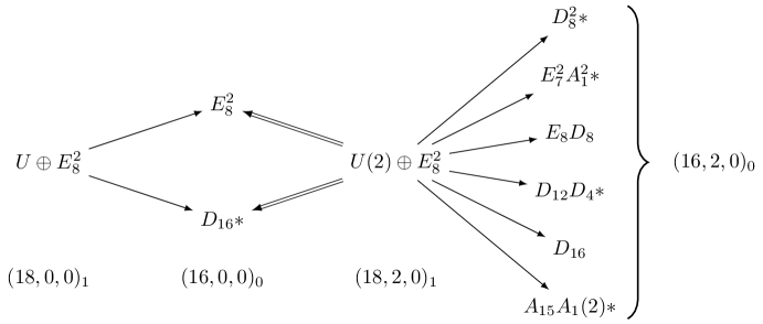
Figure 16. Cusps for $T=(20,2,0)_{2}=U\oplus U(2)\oplus E_{8}^{2}=U^{2}\oplus D_{16}$

The generic transcendental lattice is $T=S^{\perp}=(20,2,0)_{2}$. Explicitly, one has $T\simeq U\oplus U(2)\oplus E_{8}^{2}\simeq U^{2}\oplus D_{16}$. The $0$-cusps of $F_{S}$ are found by Theorem 5.8. In Fig. 1 there are two mirror moves: the odd $S=(2,2,0)\to{\overline{T}}=(18,2,0)\simeq U(2)\oplus E_{8}^{2}\simeq U\oplus D_{16}$ and the even ordinary $S=(2,2,0)\Rightarrow{\overline{T}}=(18,0,0)\simeq U\oplus E_{8}^{2}$. The $1$-cusps are given by Theorem 5.10. They correspond to the negative definite lattices ${\overline{\overline{T}}}$ with the invariants $(16,0,0)_{0}$ (i.e. unimodular) and $(16,2,0)_{0}$. These are listed in Table 2. We give the complete cusp diagram in Fig. 16. (It can also be found in [LO21].) By Proposition 5.13, the $1$-cusps for the ${\overline{\overline{T}}}(16,2,0)$ lattices are isomorphic to ${\mathbb{H}}/\operatorname{SL}(2,{\mathbb{Z}})$, and those for the ${\overline{\overline{T}}}(16,0,0)$ lattices to ${\mathbb{H}}/\Gamma_{0}(2)$.

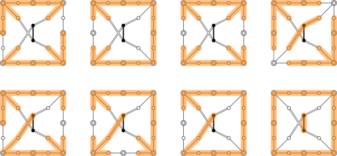
Figure 17. Maximal parabolic subdiagrams in $\Gamma_{r}$ for ${\overline{T}}=(18,2,0)$

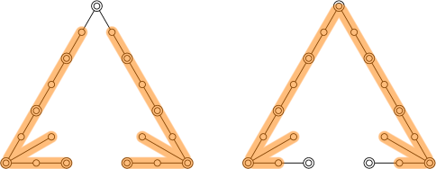
Figure 18. Maximal parabolic subdiagrams in $\Gamma_{r}$ for ${\overline{T}}=(18,0,0)$

Vinberg diagrams for ${\overline{T}}=(18,2,0)$ and ${\overline{T}}=(19,1,1)$ are given in Fig. 4. The diagram for ${\overline{T}}=(18,0,0)$ is obtained from that of $(19,1,1)$ by the procedure given in Lemma 4.15; the result is the diagram of Fig. 18 (without the highlighting). The $1$-cusps containing a given $0$-cusp correspond to the maximal parabolic subdiagrams in the Vinberg diagram. They are highlighted in Figs. 17 and 18; the order of appearance is the same as in Fig. 16.

The Kulikov models are as described in Section 8: for ${\overline{T}}=(18,2,0)$ in Section 8C and for ${\overline{T}}=(18,0,0)$ in Section 8D. The stable models are given by Theorem 9.9.

At the $(18,2,0)$ odd $0$-cusp the Type III stable models are of pumpkin type of Fig. 15. They correspond to the elliptic subdiagrams, i.e. disjoint unions of $ADE$ graphs in Fig. 17. The maximal degeneration corresponds to the empty subdiagram, or $(A^{-}_{0}\raise 0.65pt\hbox{$\kern-2.0pt\phantom{.}^{-}$}\kern-4.0ptA_{0})^{8}$. It is a union of $16$ pairs $({\mathbb{P}}^{2},D_{1}+D_{2})$ with a line $D_{1}$ and a conic $D_{2}$, as in Fig. 15. The list of irreducible components that appear, in notations of [AT21, Table 2], is as follows. We list them according to the number of the off-equator vertices. For brevity, $m$ denotes an even index and $n$ an odd index.

1. $A_{n}$ ($1\leq n\leq 15$)  $A_{m}^{-}$ ($0\leq m\leq 14$)  $\raise 0.65pt\hbox{$\kern-2.0pt\phantom{.}^{-}$}\kern-4.0ptA_{n}^{-}$ ($1\leq n\leq 15$)

2. $\kern-2.0pt\phantom{.}^{\prime}\kern-2.0pt\kern-1.0ptA_{m}^{-}$ ($2\leq m\leq 16$)  $\kern-2.0pt\phantom{.}^{\prime}\kern-2.0pt\kern-1.0ptA_{n}$ ($3\leq n\leq 15$) $D_{m}$ ($4\leq m\leq 16$)
   $D^{-}_{n}$ ($5\leq n\leq 15$) $\raise 0.65pt\hbox{$\kern-2.0pt\phantom{.}^{-}$}\kern-2.0ptE_{6}^{-}$ $\raise 0.65pt\hbox{$\kern-2.0pt\phantom{.}^{-}$}\kern-2.0ptE_{7}$ $\raise 0.65pt\hbox{$\kern-2.0pt\phantom{.}^{-}$}\kern-2.0ptE_{8}^{-}$

3. $\kern-2.0pt\phantom{.}^{\prime}\kern-2.0pt\kern-1.0ptA^{\prime}_{n}$ ($n=7,11,15$) $D^{\prime}_{n}$ ($n=9,13,17$)

4. $\kern-2.0pt\phantom{.}^{\prime}\kern-2.0pt\kern-1.0ptA^{\prime}_{3}$ $\kern-2.0pt\phantom{.}^{\prime}\kern-2.0ptD_{m}$ ($4\leq m\leq 16$) $\kern-2.0pt\phantom{.}^{\prime}\kern-2.0ptD_{n}^{-}$ ($5\leq n\leq 15$)

5. $\kern-2.0pt\phantom{.}^{\prime}\kern-2.0ptD^{\prime}_{m}$ ($m=8,12,16$)

6. $\kern-2.0pt\phantom{.}^{\prime}\kern-2.0ptD^{\prime}_{4}$

At the $(18,0,0)$ even ordinary $0$-cusp the Type III stable models are of smashed pumpkin type of Fig 15. They correspond to the elliptic subdiagrams in Fig. 18. In this case some of the irreducible components ${\overline{V}}_{i}$ are non-normal, with a long side folded $2:1$. As in [AT21, Def. 6.9], we denote these by adding the letter $f$ to the Dynkin symbol. The maximal degeneration corresponds to the empty subdiagram, or $\raise 1.17pt\hbox{$\kern-2.0pt\phantom{.}^{f}$}\kern-4.0ptA_{0}^{-}(\raise 0.65pt\hbox{$\kern-2.0pt\phantom{.}^{-}$}\kern-4.0ptA_{0}A_{0}^{-})^{7}\raise 0.65pt\hbox{$\kern-2.0pt\phantom{.}^{-}$}\kern-4.0ptA_{0}^{f}$. It is a union of $16$ pairs $({\mathbb{P}}^{2},D_{1}+D_{2})$ but in the end two of these pairs the ${\mathbb{P}}^{2}$ is glued to itself along the conic $D_{2}$ which is folded $2:1$. The list of irreducible components is as follows:

1. $\raise 0.65pt\hbox{$\kern-2.0pt\phantom{.}^{+}$}\kern-4.0ptA_{n}^{-}$ ($1\leq n\leq 15$)  $\raise 0.65pt\hbox{$\kern-2.0pt\phantom{.}^{+}$}\kern-4.0ptA_{17}^{+}$  $\raise 0.65pt\hbox{$\kern-2.0pt\phantom{.}^{+}$}\kern-4.0ptA_{m}$ ($2\leq m\leq 14)$)  $\raise 1.17pt\hbox{$\kern-2.0pt\phantom{.}^{f}$}\kern-4.0ptA_{16}^{+}$
   $\raise 1.17pt\hbox{$\kern-2.0pt\phantom{.}^{f}$}\kern-4.0ptA_{n}$ $(1\leq n\leq 13)$  $\raise 1.17pt\hbox{$\kern-2.0pt\phantom{.}^{f}$}\kern-4.0ptA^{f}_{15}$  $\raise 1.17pt\hbox{$\kern-2.0pt\phantom{.}^{f}$}\kern-4.0ptA_{m}^{-}\ (0\leq m\leq 14)$
   $\raise 0.65pt\hbox{$\kern-2.0pt\phantom{.}^{-}$}\kern-4.0ptA_{n}^{-}\ (1\leq n\leq 13)$  $\raise 0.65pt\hbox{$\kern-2.0pt\phantom{.}^{-}$}\kern-4.0ptA_{m}\ (0\leq m\leq 12)$  $A_{n}\ (1\leq n\leq 11)$.

2. $\kern-2.0pt\phantom{.}^{\prime}\kern-2.0pt\kern-1.0ptA^{+}_{4}$  $\kern-2.0pt\phantom{.}^{\prime}\kern-2.0pt\kern-1.0ptA^{+}_{16}$  $\raise 1.17pt\hbox{$\kern-2.0pt\phantom{.}^{f}$}\kern-4.0ptA^{\prime}_{3}$  $\raise 1.17pt\hbox{$\kern-2.0pt\phantom{.}^{f}$}\kern-4.0ptA^{\prime}_{15}$  $\kern-2.0pt\phantom{.}^{\prime}\kern-2.0pt\kern-1.0ptA_{m}\ (2\leq m\leq 14)$  $\kern-2.0pt\phantom{.}^{\prime}\kern-2.0pt\kern-1.0ptA_{n}\ (3\leq n\leq 13)$
   $D_{5}^{+}$ $\raise 0.65pt\hbox{$\kern-2.0pt\phantom{.}^{f}$}\kern-2.0ptD^{+}_{17}$  $\raise 0.65pt\hbox{$\kern-2.0pt\phantom{.}^{f}$}\kern-2.0ptD_{m}\ (4\leq m\leq 14)$  $\raise 0.65pt\hbox{$\kern-2.0pt\phantom{.}^{f}$}\kern-2.0ptD_{n}\ (5\leq n\leq 15)$  $\raise 0.65pt\hbox{$\kern-2.0pt\phantom{.}^{+}$}\kern-2.0ptE_{6}^{-}$  $\raise 0.65pt\hbox{$\kern-2.0pt\phantom{.}^{+}$}\kern-2.0ptE_{7}$  $\raise 0.65pt\hbox{$\kern-2.0pt\phantom{.}^{+}$}\kern-2.0ptE_{8}^{-}$

3. $\kern-2.0pt\phantom{.}^{\prime}\kern-2.0pt\kern-1.0ptA^{\prime}_{15}$

The Type II stable models are described by the maximal parabolic subdiagrams of Figs. 17, 18. The irreducible components correspond to the relevant connected components.

The normalization of ${\overline{F}}_{S}$ is semitoroidal. At the $(18,2,0)$ $0$-cusp, the semifan ${\mathfrak{F}}_{\rm ram}(18,2,0)$ is a coarsening of the Coxeter semifan ${\mathfrak{F}}_{\rm r}(18,2,0)$ and neither of them is a fan. At the $(18,0,0)$ $0$-cusp, a maximal-dimensional cone of the semifan ${\mathfrak{F}}_{\rm ram}(18,0,0)$ is a union of $4$ maximal-dimensional cones of ${\mathfrak{F}}_{\rm r}(18,0,0)={\mathfrak{F}}_{2}(18,0,0)$, and both of them are fans, so near this cusp the normalization of ${\overline{F}}_{S}$ is toroidal.

References

- [ABE22] Valery Alexeev, Adrian Brunyate, and Philip Engel, Compactifications of moduli of elliptic K3 surfaces: stable pair and toroidal, Geom. and Topology 26 (2022), no. 8, 3525–3588, arXiv:2002.07127.
- [AE21] Valery Alexeev and Philip Engel, Compact moduli of K3 surfaces, Annals of Math., to appear (2021), arXiv:2101.12186.
- [AEH21] Valery Alexeev, Philip Engel, and Changho Han, Complete moduli of K3 surfaces with a nonsymplectic automorphism, Trans. Amer. Math. Soc., to appear (2021), arXiv:2110.13834.
- [AET19] Valery Alexeev, Philip Engel, and Alan Thompson, Stable pair compactification of moduli of K3 surfaces of degree 2, J. Reine Angew. Math., to appear (2019), arXiv:1903.09742.
- [AMRT75] A. Ash, D. Mumford, M. Rapoport, and Y. Tai, Smooth compactification of locally symmetric varieties, Math. Sci. Press, Brookline, Mass., 1975, Lie Groups: History, Frontiers and Applications, Vol. IV.
- [AN06] Valery Alexeev and Viacheslav V. Nikulin, Del Pezzo and surfaces, MSJ Memoirs, vol. 15, Mathematical Society of Japan, Tokyo, 2006, arXiv:math/0406536.
- [AT21] Valery Alexeev and Alan Thompson, ADE surfaces and their moduli, J. Algebraic Geometry 30 (2021), 331–405, arXiv:1712.07932.
- [CD89] François R. Cossec and Igor V. Dolgachev, Enriques surfaces. I, Progress in Mathematics, vol. 76, Birkhäuser Boston, Inc., Boston, MA, 1989.
- [Cox35] H. S. M. Coxeter, Wythoff’s Construction for Uniform Polytopes, Proc. London Math. Soc. (2) 38 (1935), 327–339.
- [CS99] J. H. Conway and N. J. A. Sloane, Sphere packings, lattices and groups, third ed., Grundlehren der Mathematischen Wissenschaften [Fundamental Principles of Mathematical Sciences], vol. 290, Springer-Verlag, New York, 1999, With additional contributions by E. Bannai, R. E. Borcherds, J. Leech, S. P. Norton, A. M. Odlyzko, R. A. Parker, L. Queen and B. B. Venkov.
- [DK07] Igor V. Dolgachev and Shigeyuki Kondō, Moduli of surfaces and complex ball quotients, Arithmetic and geometry around hypergeometric functions, Progr. Math., vol. 260, Birkhäuser, Basel, 2007, pp. 43–100.
- [Dol96] I. V. Dolgachev, Mirror symmetry for lattice polarized surfaces, J. Math. Sci. 81 (1996), no. 3, 2599–2630, Algebraic geometry, 4.
- [EF21] Philip Engel and Robert Friedman, Smoothings and rational double point adjacencies for cusp singularities, J. Differential Geom. 118 (2021), no. 1.
- [Eng18] Philip Engel, Looijenga’s conjecture via integral-affine geometry, J. Differential Geom. 109 (2018), no. 3, 467–495.
- [FM83] Robert Friedman and Rick Miranda, Smoothing cusp singularities of small length, Math. Ann. 263 (1983), no. 2, 185–212.
- [Fri83] Robert Friedman, Global smoothings of varieties with normal crossings, Ann. of Math. (2) 118 (1983), no. 1, 75–114.
- [FS86] Robert Friedman and Francesco Scattone, Type degenerations of surfaces, Invent. Math. 83 (1986), no. 1, 1–39.
- [GHK15] Mark Gross, Paul Hacking, and Sean Keel, Moduli of surfaces with an anti-canonical cycle, Compos. Math. 151 (2015), no. 2, 265–291.
- [GS03] Mark Gross and Bernd Siebert, Affine manifolds, log structures, and mirror symmetry, Turkish J. Math. 27 (2003), no. 1, 33–60.
- [Kim18] Yusuke Kimura, K3 surfaces without section as double covers of Halphen surfaces, and F-theory compactifications, PTEP. Prog. Theor. Exp. Phys. (2018), no. 4, 043B06, 13.
- [Kim20] by same author, in F-theory on K3 surfaces without section as double covers of Halphen surfaces, Adv. Theor. Math. Phys. 24 (2020), no. 2, 459–490.
- [Kol23] János Kollár, Families of varieties of general type, Cambridge Tracts in Mathematics, vol. 231, Cambridge University Press, Cambridge, 2023.
- [Kon89] Shigeyuki Kondō, Algebraic surfaces with finite automorphism groups, Nagoya Math. J. 116 (1989), 1–15.
- [KS06] Maxim Kontsevich and Yan Soibelman, Affine structures and non-Archimedean analytic spaces, The unity of mathematics, Progr. Math., vol. 244, Birkhäuser Boston, Boston, MA, 2006, arXiv: math.AG/0406564, pp. 321–385.
- [Kul77] Vik. S. Kulikov, Degenerations of surfaces and Enriques surfaces, Izv. Akad. Nauk SSSR Ser. Mat. 41 (1977), no. 5, 1008–1042, 1199.
- [LO21] Radu Laza and Kieran O’Grady, GIT versus Baily-Borel compactification for ’s which are double covers of , Adv. Math. 383 (2021), Paper No. 107680, 63.
- [Loo03] Eduard Looijenga, Compactifications defined by arrangements. II. Locally symmetric varieties of type IV, Duke Math. J. 119 (2003), no. 3, 527–588.
- [MP86] Rick Miranda and Ulf Persson, On extremal rational elliptic surfaces, Math. Z. 193 (1986), no. 4, 537–558.
- [Nik79a] V. V. Nikulin, Integer symmetric bilinear forms and some of their geometric applications, Izv. Akad. Nauk SSSR Ser. Mat. 43 (1979), no. 1, 111–177, 238.
- [Nik79b] by same author, Quotient-groups of groups of automorphisms of hyperbolic forms of subgroups generated by -reflections, Dokl. Akad. Nauk SSSR 248 (1979), no. 6, 1307–1309.
- [Nik81] by same author, Quotient-groups of groups of automorphisms of hyperbolic forms by subgroups generated by -reflections. Algebro-geometric applications, Current problems in mathematics, Vol. 18, Akad. Nauk SSSR, Vsesoyuz. Inst. Nauchn. i Tekhn. Informatsii, Moscow, 1981, pp. 3–114.
- [Nik20] Viacheslav V. Nikulin, Some examples of K3 surfaces with infinite automorphism group which preserves an elliptic pencil, Math. Notes 108 (2020), no. 3-4, 542–549.
- [OS91] Keiji Oguiso and Tetsuji Shioda, The Mordell-Weil lattice of a rational elliptic surface, Comment. Math. Univ. St. Paul. 40 (1991), no. 1, 83–99.
- [Per90] Ulf Persson, Configurations of Kodaira fibers on rational elliptic surfaces, Math. Z. 205 (1990), no. 1, 1–47.
- [PP81] Ulf Persson and Henry Pinkham, Degeneration of surfaces with trivial canonical bundle, Ann. of Math. (2) 113 (1981), no. 1, 45–66.
- [Sca87] Francesco Scattone, On the compactification of moduli spaces for algebraic surfaces, Mem. Amer. Math. Soc. 70 (1987), no. 374, x+86.
- [Sym03] Margaret Symington, Four dimensions from two in symplectic topology, Topology and geometry of manifolds (Athens, GA, 2001), Proc. Sympos. Pure Math., vol. 71, Amer. Math. Soc., Providence, RI, 2003, pp. 153–208.
- [Vin72] È. B. Vinberg, The groups of units of certain quadratic forms, Mat. Sb. (N.S.) 87(129) (1972), 18–36.
- [Vin75] È. B. Vinberg, Some arithmetical discrete groups in Lobačevskiĭ spaces, Discrete subgroups of Lie groups and applications to moduli (Internat. Colloq., Bombay, 1973), Oxford Univ. Press, Bombay, 1975, pp. 323–348.
- [Vin83] È. B. Vinberg, The two most algebraic surfaces, Math. Ann. 265 (1983), no. 1, 1–21.
- [VK78] È. B. Vinberg and I. M. Kaplinskaja, The groups and , Dokl. Akad. Nauk SSSR 238 (1978), no. 6, 1273–1275.
- [Zan20] Aline Zanardini, Explicit constructions of Halphen pencils, Preprint (2020), arXiv:2008.08128.