TOI-1468: A system of two transiting planets, a super-Earth and a mini-Neptune, on opposite sides of the radius valley

We report the discovery and characterization of two small transiting planets orbiting the bright M3.0 V star TOI-1468 (LSPM J0106+1913), whose transit signals were detected in the photometric time series in three sectors of the TESS mission. We confirm the planetary nature of both of them using precise radial velocity measurements from the CARMENES and MAROON-X spectrographs, and supplement them with ground-based transit photometry. A joint analysis of all these data reveals that the shorter-period planet, TOI-1468 b ($P_{\rm b}$ = 1.88 d), has a planetary mass of $M_{\rm b}=3.21\pm 0.24$ $M_{\oplus}$ and a radius of $R_{\rm b}=1.280^{+0.038}_{-0.039}\,R_{\oplus}$, resulting in a density of $\rho_{\rm b}=8.39^{+1.05}_{-0.92}$ g cm^-3, which is consistent with a mostly rocky composition. For the outer planet, TOI-1468 c ($P_{\rm c}=15.53$ d), we derive a mass of $M_{\rm c}=6.64^{+0.67}_{-0.68}$ $M_{\oplus}$, a radius of $R_{\rm c}=2.06\pm 0.04\,R_{\oplus}$, and a bulk density of $\rho_{c}=2.00^{+0.21}_{-0.19}$ g cm^-3, which corresponds to a rocky core composition with a H/He gas envelope. These planets are located on opposite sides of the radius valley, making our system an interesting discovery as there are only a handful of other systems with the same properties. This discovery can further help determine a more precise location of the radius valley for small planets around M dwarfs and, therefore, shed more light on planet formation and evolution scenarios.

1 Introduction

A number of space-based transit surveys such as CoRoT (Baglin et al., 2006), Kepler (Borucki et al., 2010), and now TESS (Ricker et al., 2015), have been able to determine precise orbital periods and radii of several thousands of exoplanets. Combining the transit light curves with radial-velocity (RV) measurements yields the planet density, as well as a complete set of orbital parameters. Currently, the total number of confirmed exoplanets is more than 5000, resulting in a broad range of measured planet bulk densities, giving us the first hints about the internal composition of planets, which is a crucial element for our understanding of their formation. One of the most important results from these discoveries is the large amount of planets with radii smaller than the radius of Neptune but larger than that of the Earth ($R_{\rm p}\approx$ 1–3.9 $R{{}_{\oplus}}$) (Batalha et al., 2013). However, until the advent of TESS, most of these exoplanets had been detected around solar-type stars, while a complete picture of the process of planet formation requires an understanding of the architecture around all types of stars.

Solar-type stars have been the prime targets of many transit searches. Some examples of initial RV surveys that focused on later stars, down to M dwarf spectral types, were the survey of high-metallicity stars (N2K; Fischer et al. 2005) and the California planet survey (Howard et al., 2010). With advancements in space-based transit missions and higher-precision RV measurements with a broader wavelength coverage, especially toward the red end of the spectrum, such as with the CARMENES (Quirrenbach et al., 2014) and the MAROON-X (Seifahrt et al., 2018, 2020) spectrographs, we are starting to shift the focus toward M dwarfs, the most abundant stars in our galaxy (Chabrier, 2003; Henry et al., 2018; Reylé et al., 2021).

One of the main advantages of late-type dwarfs over solar-type stars are the relative sizes and masses between the host-stars and their planets, which make these systems more detectable via transit and RV techniques. This fact has been exploited by surveys that have exclusively focused on searches for planets around M dwarfs, such as the SPIRou Legacy Survey (Cloutier et al., 2018), the M dwarfs in the Multiples survey with Subaru (Ward-Duong et al., 2015), and similar such surveys with UVES, HARPS, CARMENES, and other instruments (Kürster et al., 2003; Charbonneau et al., 2008; Zechmeister & Kürster, 2009; Bonfils et al., 2013; Reiners et al., 2018).

Transiting planet discoveries have shown that planetary interiors can be quite diverse, ranging from completely rocky cores to gas-dominated planets. They have also indicated a higher frequency for low-mass planets ($1\,M_{\oplus}\lesssim M_{\rm p}\sin{i}\lesssim 10\,M_{\oplus}$) around low-mass stars ($M_{\odot}\lesssim 0.6\,M_{\oplus}$) in orbits less than 100 d, compared to solar-type stars (Howard et al., 2012; Dressing & Charbonneau, 2013; Hsu et al., 2020). In a recent study, Sabotta et al. (2021) found an occurrence rate of $1.32^{+0.33}_{-0.31}$ low-mass planets for low-mass stars in periods up to 100 d. Detailed studies of several of these planets occurring around solar-type stars have revealed a bimodal distribution of planets peaking at 1.3 $R_{\oplus}$ and 2.6 $R_{\oplus}$, and consequently a relative paucity of planets between 1.5 $R_{\oplus}$ and 1.8 $R_{\oplus}$, also known as the radius valley (Fulton et al., 2017; Zeng et al., 2017; Van Eylen et al., 2018; Berger et al., 2018).

One of the explanations for this bimodal distribution is the formation of planets in a gas-poor environment. In this scenario, the inner disk, where the planets form, is clear of H gas (Owen & Wu, 2013). Thus, irrespective of the mass of the planet, and in absence of such gases, the close-in planets cannot accrete H and He. However, a planet that formed further away from its host star and subsequently migrated inward may then be able to keep its H+He envelope. Nevertheless, not all systems can be explained in this way. Systems such as K2–3 (Damasso et al., 2018) and TOI-1266 (Stefánsson et al., 2020), where the inner planets are larger than the outer planets, defy these assumptions. These systems could instead be explained by assuming that the outer planets had a richer water ice composition (Owen & Campos Estrada, 2020).

Another explanation is that all planets are formed with an H atmosphere but they lose it during the course of evolution, mainly in the first 100 Ma after formation (Lammer et al., 2014; Linsky & Güdel, 2015). Here, the accreted H+He envelope is removed due to the extreme ultraviolet (XUV) radiation of the host star (Sanz-Forcada et al., 2011; Owen & Wu, 2013; López & Fortney, 2013). The erosion depends on the surface gravity of the planet, its separation from the host star, and the amount of XUV radiation that the planet has received during its lifetime. The outer atmospheres for planets with masses less than 10 $M_{\oplus}$, or orbiting very close to the host stars, can be easily eroded by the XUV radiation coming from the host star, especially if the host star is active. The activity of M stars increases toward the latest spectral type (Reiners et al., 2012) and, since the lifetimes of these stars are also long, they can be in a relatively high-activity phase for a long time. As a result, planet atmosphere losses due to XUV erosion can be particularly high. Alternatively, the atmospheric losses would be less if the star was relatively inactive when it was young. In a third scenario, where atmospheric losses are driven by the energy release from the formation process (Ginzburg et al., 2018; Gupta & Schlichting, 2019, 2020), the H+He envelope is removed because young, rocky planets are very hot. The removal of the envelope typically takes place on the order of 1 Ga. Since the planet is the driving force, this loss mechanism should also be relevant for planets orbiting at large separations from their host stars. Additionally, Ginzburg et al. (2018) and Gupta & Schlichting (2019) also predicted that the location of the radius valley should decrease with orbital period as $R_{\rm valley}\sim P^{-0.13}$. It is possible that all these processes are relevant for the evolution of the planets. However, one process could be more relevant for planets orbiting a specific type of star than for another.

In this paper, we present the discovery of a multi-planetary system with at least two transiting planets around an early-to-mid-type M dwarf, LSPM J0106+1913 (Lépine & Shara, 2005), recently cataloged as TOI-1468. The paper is organized as follows. In Sect. 2, we describe the space-based photometry from TESS. Section 3 comprises all the ground-based observations including additional photometry, high-resolution imaging, and CARMENES high-resolution spectroscopy. In Sect. 4, we discuss the host star by listing its stellar properties and investigating the rotational period of the star. In Sect. 5, we discuss the detailed modeling of the RV and transit data, and the obtained results. We finally interpret our results in Sect. 6 and present a brief summary in Sect. 7.

2 TESS photometry

2.1 Transit search

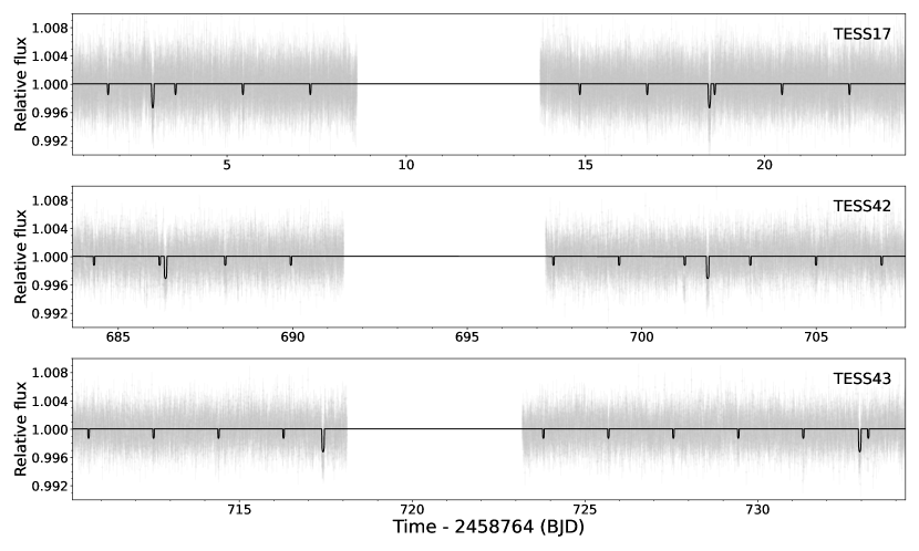
Figure 1: TESS PDCSAP light curve for TOI-1468 (gray points) for three sectors: 17, 42, and 43, overplotted with the two-transiting-planet model in black.

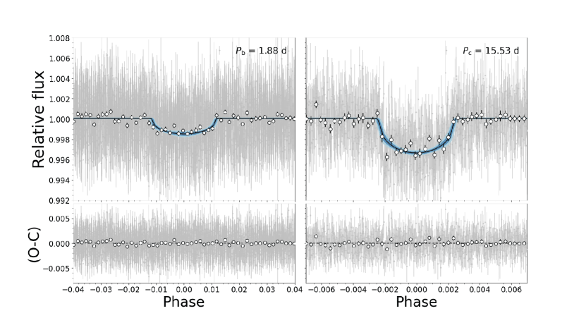
Figure 2: Phase-folded TESS transit light curves for TOI-1468 b at 1.88 d (left) and TOI-1468 c at 15.53 d (right). Gray points are 2 min (and 20 s) cadence data, and open circles are binned data (shown only for reference; data used to fit the model were the unbinned points). The best-fit juliet model (black line; see Sect. 5) is overplotted for both TOI-1468 b and TOI-1468 c, along with shaded regions, light blue for $95\,\%$ and dark blue for $68\,\%$ confidence intervals.

The TESS mission was designed to perform an all-sky survey to detect transiting planets using its four cameras, each having a field of view of $24\,\times\,24$ deg² outfitted with four 2k $\times$ 2k CCDs (charge-coupled devices). The light curves are archived in raw and processed format in the Mikulski Archive for Space Telescopes. TIC 243185500 (discovery name: LSPM J0106+1913) was observed at 2 min short-cadence integrations in sector 17. The data validation report (Twicken et al., 2018; Li et al., 2019) produced by the TESS Science Processing Operations Center (SPOC; Jenkins et al., 2016)) identified transit signals with orbital periods of 1.88 d and 15.53 d. The target star was subsequently promoted to TESS Object of Interest (TOI) status as TOI-1468 by the TESS Science Office; the associated planet candidates were designated as TOI-1468.01 (15.53 d) and TOI-1468.02 (1.88 d) (Guerrero et al., 2021). Finally, TOI 1468 was observed at 2 min (and 20 s) cadence in extended mission sectors 42 and 43 (see Table 1 for details). The transit depths for the inner and outer planets are 1.66 mmag and 3.73 mmag, respectively.

We show the TESS SPOC pre-search data conditioning simple aperture photometry (PDCSAP) (Smith et al., 2012; Stumpe et al., 2012, 2014) for sectors 17, 42, and 43 observed for both transiting planets in Fig. 1. Phase-folded and best-fit models for both planets are shown in Fig. 2 (see Sect. 5.2 for detailed analysis.)

Table 1: TESS observations of TOI-1468.

Sector	Camera	Cycle	Start date	End date
17	1	2	07 October 2019	02 November 2019
42	3	4	20 August 2021	16 September 2021
43	1	4	16 September 2021	12 October 2021

2.2 Limits on photometric contamination

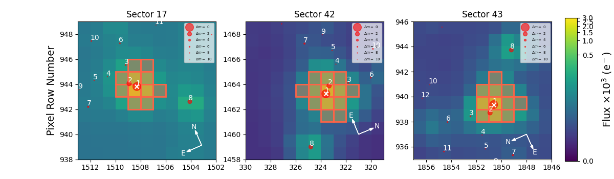
Figure 3: Target pixel files of TOI-1468 in TESS sectors 17, 42, and 43. The electron counts are color-coded. The red-bordered pixels are used in the simple aperture photometry. The size of the red circles indicates the TESS magnitudes of all nearby stars and TOI-1468 (circle $\#$1 marked with «$\times$»).

The large TESS pixel size of $\sim 21$ arcsec increases the likelihood of contamination by nearby stars. In Fig. 3, we plot all the Gaia sources within the field of view of the TESS aperture with the help of tpfplotter (Aller et al., 2020). The advantage of this comparison is that both the Gaia $G_{RP}$ band (630–1050 nm) and the TESS $T$ band (600–1000 nm) have a similar wavelength coverage. The SPOC crowding metric for TOI-1468 in the three TESS sectors was $\sim$0.91. This means that according to SPOC modeling after background removal, $\sim 91\,\%$ of the flux in the photometric aperture was attributable to the target star, and $\sim 9\,\%$ to other sources, especially to source #2 (TIC 243185499, Gaia EDR3 2785466581298775552), which is separated from TOI-1468 by $\sim$14 arcsec and is 1.7 mag fainter in the $G$ band. The PDCSAP flux level was reduced to account for contamination by other sources, as described in the SPOC PDCSAP references. The high-resolution imaging data for ascertaining any resolved close multiplicity of TOI-1468 is described in Sect. 3.3.

3 Ground-based observations

3.1 Ground-based photometry

Several targeted observations of TOI-1468 were scheduled to monitor the transits for both planetary candidates with various ground-based facilities. The summary description of all the observed transits is given in Table 2. We further examined archival time-series photometry data of TOI-1468 and listed these observations in Table 4. The photometric data of each facility, phase-folded to the best-fit model (Sect. 5), are shown in Fig. 4 for TOI-1468 b and in Fig. 5 for TOI-1468 c. All the data sets were modeled with the juliet package and the best-fit model is overplotted in each of the panels (see Sect. 5.2 for details). In the following paragraphs, we describe the eventually used photometric ground-based photometric data for TOI-1468. Unused data sets, either from archival or follow-up observations (i.e., MEarth, TRAPPIST, FLWO, GMU), did not have enough quality for the relatively shallow transits of TOI-1468 b and c.

Table 2: Ground-based observations of TOI-1468 transits.

Planet	Telescope	Camera or	Filter	Pixel scale	PSFa	Aperture	Date	Duration	Used
		instrument		(arcsec)	(arcsec)	radius (pixel)	(UT)	(min)	data setb
b	MEarth-N (0.4 m)	Apogee U42	$RG715$	0.75	3.2	8.0	2019-12-12	384.0	…
b	MEarth-Nx7 (0.4 m)	Apogee U42	$RG715$	0.76	6.9	9.0	2019-12-12	385.0	…
b	MEarth-S (0.4 m)	Apogee U/F230	$RG715$	0.84	2.2	4.2	2019-12-12	206.0	…
b	TCS (1.52 m)	MuSCAT2	$g$, $r$, $i$, $z_{s}$	0.44	11.8c	…	2019-12-13	174.6	…
b	TRAPPIST-N (0.60 m)	Andor IKON-L BEX2-DD	$z$	0.60	3.0	6.01	2019-12-13	210.0	…
c	MEarth-S (0.4 m)	Apogee U/F230	$RG715$	0.84	2.2	6.0	2019-12-27	137.0	…
c	MEarth-Sx6 (0.4 m)	Apogee U/F230	$RG715$	0.84	5.1	9.9	2019-12-27	140.0	…
c	SO-Kuiper (1.5 m)	Mont4k	$B$	0.42	…	…	2020-01-27	176.0	Yes
c	FLWO (1.2 m)	KeplerCam	$i$	0.672	2.2	6.0	2020-01-27	148.0	…
b	LCOGT-SAAO (1.0 m)	Sinistro	$g_{p}$	0.389	2.73	12.0	2020-07-19	229.0	Yes
b	LCOGT-SAAO (1.0 m)	Sinistro	$g_{p}$	0.389	1.81	10.0	2020-08-19	256.0	Yes
b	LCOGT-SSO (1.0 m)	Sinistro	$z_{s}$	0.39	1.93	15.0	2020-08-27	252.0	Yes
c	LCOGT-SSO (1.0 m)	Sinistro	$z_{s}$	0.39	2.71	13.0	2020-10-01	281.0	Yes
b	GMU (0.8 m)	SBIG STX-16803+FW-7	$R$	0.36	5.34	15.0	2020-10-06	194.0	…
b	LCOGT-SSO (1.0 m)	Sinistro	$i_{p}$	0.389	4.58	17.0	2020-10-15	277.0	Yes
c	LCOGT-McD (1.0 m)	Sinistro	$i_{p}$	0.39	2.71	11.0	2020-10-17	317.0	Yes
b	LCOGT-SAAO (1.0 m)	Sinistro	$i_{p}$	0.39	4.33	14.0	2020-10-24	337.0	Yes
b	LCOGT-McD (1.0 m)	Sinistro	$i_{p}$	0.389	7.47	21.0	2020-11-22	303.0	Yes
b	TCS (1.52 m)	MuSCAT2	$g$, $i$, $z{{}_{s}}$	0.44	11.8c	…	2021-07-14	116.0	Yes
b	TCS (1.52 m)	MuSCAT2	$g$, $i$, $z{{}_{s}}$	0.44	11.8c	…	2021-08-30	161.0	Yes

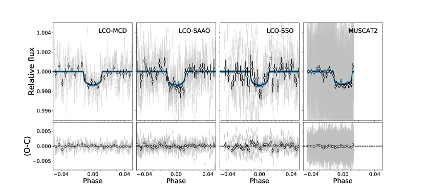
Figure 4: Ground-based photometry data for TOI-1468 b was observed from various facilities, namely, LCO-McD, LCO-SAAO, LCO-SSO, and MUSCAT2. The normalized flux data are plotted in gray points, with the binned data points highlighted by circles, along with their error bars. The number of data points per bin was ten for LCO-McD, LCO-SAAO, LCO-SS0, and 30 for MUSCAT2. The juliet best-fit model for each set is plotted as a solid black line, along with shaded regions: light blue for the $95\%$ confidence interval, and dark blue for the $68\%$ confidence interval. Details can be found in Sect. 5. The residuals are plotted in the bottom part of each of the panels.

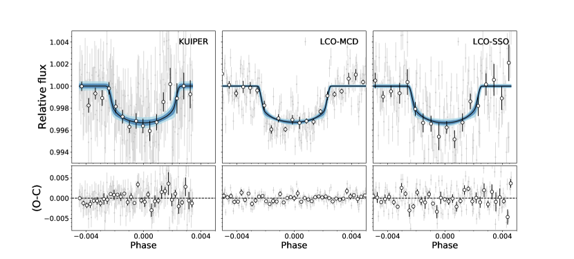
Figure 5: Ground-based photometry data for TOI-1468 c observed from various facilities, namely, SO-KUIPER, LCO-McD, and LCO-SSO. The normalized flux data are plotted in gray, with the binned data in circles, along with their error bars. The number of data points per bin was ten. The juliet best-fit model for each set is plotted as a solid black line, along with shaded regions: light blue for the $95\%$ confidence interval, and dark blue for the $68\%$ confidence interval. The residuals are plotted in the bottom part of each of the panels.

LCOGT.

Las Cumbres Global Telescope Network (LCOGT; Brown et al., 2013) is a network of 0.4 -meter, 1-meter, and 2-meter fully automated robotic telescopes spread across the globe. We recorded eight transits of TOI-1468 with three 1-meter telescopes of the LCOGT network and three different filters ($g_{p}$, $z_{s}$, $i_{p}$). In particular, we observed six transits of TOI-1468 b and two transits of TOI-1468 c at the LCOGT South African Astronomical Observatory (SAAO) in South Africa on 19 July 2020, 19 August 2020, and 24 October 2020, at the LCOGT Siding Spring Observatory (SSO) in Australia) on 27 August 2020, 01 October 2020, and 15 October 2020, and at the LCOGT McDonald (McD) Observatory, in the USA on 17 October 2020 and 22 November 2020. Observation durations varied between 229 min and 337 min, significantly longer than the transit durations ($\sim$73–108 min).

The data were reduced with the automated Python-based BANZAI pipeline (McCully et al., 2018). The pipeline performs the standard process of data reduction, including the removal of bad pixels, bias subtraction, dark subtraction, flat-field correction, source extraction photometry (with Python and C libraries), and astrometric calibration (with astrometry.net). Aperture photometry radii varied depending on the local seeing, between 4.3 arcsec and 6.6 arcsec. The transit data were further analyzed using the AstroImageJ (AIJ) software (Collins et al., 2017) and airmass detrended for all the datsets.

SO-Kuiper.

The 61-inch Kuiper telescope is operated by the Steward Observatory and is located at 2500 m at Mt. Bigelow in the Catalina Mountains north of Tucson, Arizona (USA). The 4k $\times$ 4k Mont4K CCD was used for the imaging to monitor a single transit of TOI-1468 c with a $B$ filter on 27 January 2020. The target star was observed for a duration of 4.5 h with an average seeing of $\sim$ 3 arcsec. The SO-Kuiper data reduction was done with publically available Python pipeline (Weiner et al., 2018), which is based on IRAF’s (Tody, 1993) ccdproc and follows the basic reduction steps of overscan, trim, bias, and flat field correction. Further analysis was done with the AIJ software using the fixed aperture of four pixels.

MuSCAT2.

We observed two transits of TOI-1468 b simultaneously in $g$, $r$, $i$, and $z_{\mathrm{s}}$ bands with the MuSCAT2 multicolor imager (Narita et al., 2019) installed on the 1.52-meter Telescopio Carlos Sánchez (TCS) at the Observatorio del Teide, Tenerife (Spain). The observations were carried out on the nights of 14 July 2021 and 30 August 2021, with exposure times optimized each night and per passband, and varied from 10 s to 30 s. The airmass varied from a minimum of 1.1 to a maximum of 1.5 during the first night, and from a minimum of 1.01 to a maximum of 1.13 during the second night. The observing conditions were good through both nights, but the scatter in photometry was higher than expected. This high scatter is likely attributed to high levels of atmospheric dust. The photometry was conducted using standard aperture photometry calibration and reduction steps with a dedicated MuSCAT2 photometry pipeline, as described in Parviainen et al. (2019). The pipeline calculates aperture photometry for the target and a set of comparison stars and aperture sizes, and creates the final relative light curves via global optimization of a model that aims to find the optimal comparison stars and aperture size, while simultaneously modeling the transit and baseline variations modeled as a linear combination of a set of covariates.

3.2 High-resolution spectroscopy

The high-resolution spectroscopic data used for this paper were obtained with CARMENES, fiber-coupled to the Cassegrain focus of the 3.5-meter telescope at the Observatorio de Calar Alto in Almería (Spain), and MAROON-X, a new extreme precision RV spectrograph at the 8.1 m Gemini North telescope in Maunakea, Hawai’i (USA).

3.2.1 CARMENES

CARMENES is a dual channel spectrograph operating in the optical wavelength band (VIS) between 0.52 $\mu$m and 0.96 $\mu$m, with a spectral resolving power of $\mathcal{R}$ = 94 600, and in the near-infrared (NIR) between 0.96 $\mu$m and 1.71 $\mu$m at $\mathcal{R}$ = 80.400. With CARMENES, we obtained 65 spectra for TOI-1468 between 20 January 2020 and 09 October 2020. The exposure times were 1800 s. The spectra followed the standard data flow (Caballero et al., 2016) and were reduced with caracal (Zechmeister et al., 2014), while the RVs were produced with serval (Zechmeister et al., 2018). The reduction included the standard process of barycentric and instrumental drifts corrections. serval produces RVs were nightly-zero-point corrected as discussed by Kaminski et al. 2018, Tal-Or et al. 2019, and especially, Trifonov et al. 2020. Additional information, such as spectral activity indices, were also produced, as part of the science products from serval, such as the CRX chromatic index (VIS and NIR) and dLW, the differential line width. Following the method of Schöfer et al. (2019), we additionally computed $\log{L_{{\rm H}\alpha}/L_{\rm bol}}$ and a number of atomic and molecular indices (H$\alpha$, He i D₃, Na i D₁ and D₂, Ca ii IRT1, -2, and -3, He i $\lambda$10833 Å, Pa$\beta$, CaH-2, CaH-3, TiO 7050, TiO 8430, TiO 8860, VO 7436, VO 7942, and FeH Wing-Ford). The average signal-to-noise ratio (S/N) of the CARMENES spectra is 61 at 740 nm, measured at the peak of the blaze function. The median error and the scatter of the time series of the VIS RVs are 2.0 m s^-1 and $\sigma$ = 4.7 m s^-1, respectively, while those of the NIR RVs are 8.0 m s^-1 and $\sigma$ = 9.8 m s^-1, respectively. The median errors on NIR RV data were larger than the predicted RV semi-amplitude, $K\sim$ 3–4 m s^-1), and therefore we only used VIS RVs for all of our further analyses. The CARMENES RVs, along with their uncertainties and their respective BJD time stamps, are listed in Table 9.

3.2.2 MAROON-X

MAROON-X is a stabilized, fiber-fed échelle spectrograph, with a resolving power of $\mathcal{R}\,=\,85\,000$ and a wavelength range of 0.50–0.92 $\mu$m covered by two arms. MAROON-X demonstrated an RV stability of at least 30 cm s^-1 over the span of a few weeks during its first year of operations (Seifahrt et al., 2020) and was used to determine the precise mass of the nearby transiting rocky planet Gl 486 b (Trifonov et al., 2021). We obtained 16 spectra of TOI-1468 in two observing runs in August and October-November 2021. The exposure time was typically 600 s. The RVs from both runs were treated as independent data sets with their own RV offset. The spectra were reduced with a custom package and the RVs were produced with a Python 3 implementation of serval (Zechmeister et al., 2018). One-dimensional spectra and RVs were computed separately for the blue and red arms of MAROON-X. Barycentric corrections were calculated for the flux-weighted midpoint of each observation. Wavelength solutions and instrumental drift corrections were based on the MAROON-X etalon calibrator. In August 2021, an additional ad hoc drift correction of 0.19 m s^-1 day^-1 was applied, based on consistent systematics found in the observations of multiple RV standard stars. As for CARMENES, additional information, such as spectral activity indicators (CRX and dLW), as well as line indices for H$\alpha$, Na i D, and Ca ii IRT1, -2, and -3, were computed. Average S/N (at the peak of the blaze) for the spectra of TOI-1468 are $\sim$50 at 640 nm in the blue arm and $\sim$125 at 800 nm in the red arm. These large rations resulted in average RV uncertainties of 1.8 m s^-1 for the blue arm and 0.95 m s^-1 for the red arm of MAROON-X. The RVs, along with their uncertainties and activity indicators, are listed in Table 10

3.3 High-resolution imaging

For TOI-1468, the Gaia EDR3 renormalized unit weight error (RUWE) value is 1.62, which is slightly above the critical value of 1.40. This value might hint that the source could be non-single or problematic for the photometric solution (Arenou et al., 2018; Lindegren et al., 2018). Due to the RUWE value and the large pixel size of TESS, we obtained Gemini high-resolution speckle imaging in the visible, and Palomar adaptive optics imaging in the near-infrared, to detect and measure the contribution of any contaminating sources near TOI-1468.

3.3.1 Gemini

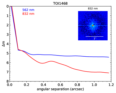
Figure 6: ‘Alopeke 832 nm reconstructed image of TOI-1468 and 5$\sigma$ contrast curves for the simultaneous observations at 562 nm (blue) and 832 nm (red).

TOI-1468 was observed on 04 August 2020 with the ‘Alopeke speckle imager mounted on the 8.1-meter Gemini North telescope. The data were simultaneously acquired in two bands centered at 562 nm and 832 nm, with filter bandwidths of 54 nm and 40 nm, respectively, on which eight sets of 1000 $\times$ 0.06 s exposures were obtained. The images were reduced, as discussed by Howell et al. (2011). The inner working angle (which is equal to the diffraction limit) is 0.02 arcsec at 562 nm and 0.03 arcsec at 832 nm. The inner spatial resolution is $\sim$0.5–0.7 au at the TOI-1468 distance. Between 0.1 arcsec and 1.2 arcsec, we excluded nearby stars fainter than $\sim$5 mag at 562 nm and $\sim$5–7 mag at 832 nm, as shown in Fig. 6.

3.3.2 Palomar

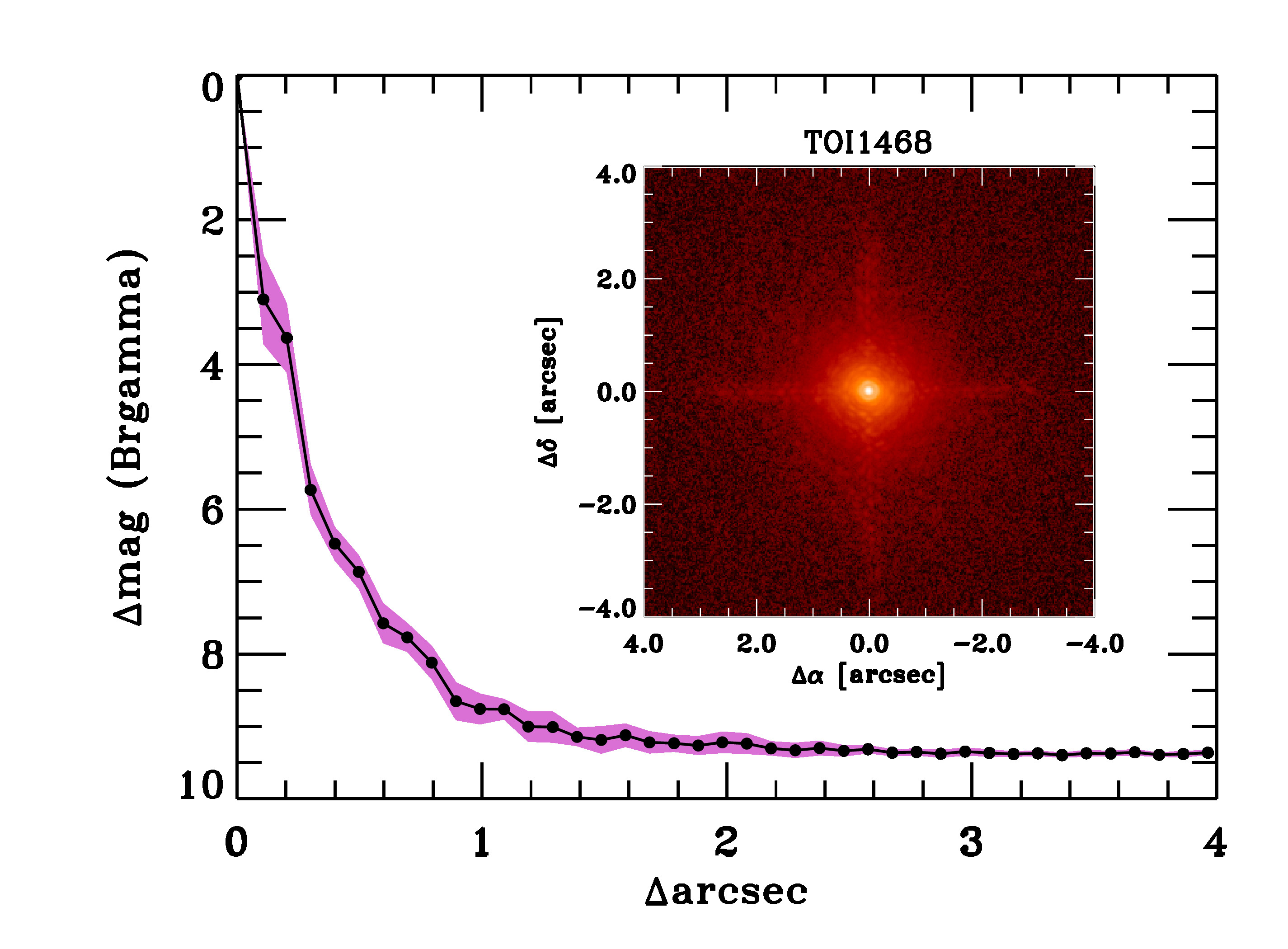
Figure 7: Palomar PHARO Br$\gamma$ image of TOI-1468 and contrast curve ($5\sigma$ limits in black dots, rms dispersion in magenta).

Deeper high-resolution imaging observations of TOI-1468 were made at the 200-inch Hale telescope of the Palomar Observatory. On 08 Aug 2021, we used the PHARO instrument (Hayward et al., 2001) behind the natural guide star adaptive optics system P3K (Dekany et al., 2013) in a standard five-point quincunx dither pattern with steps of 5 arcsec in the narrow-band Br$\gamma$ filter ($\lambda_{0}$ = 2168.6 nm, $\Delta\lambda$ = 32.6 nm). Each dither position was observed three times, offset in position from each other by 0.5 arcsec for a total of 15 frames, with an integration time of 9.9 s per frame, for a total on-source time of 148 s. The images were taken in good seeing conditions. PHARO has a pixel scale of 0.025 arcsec per pixel for a total field of view of $\sim$25 arcsec.

The science frames were flat-fielded and sky-subtracted. The flat fields were generated from a median average of dark subtracted flats taken on-sky. The flats were normalized such that the median value of the flats was unity. The sky frames were generated from the median average of the 15 dithered science frames; each science image was then sky-subtracted and flat-fielded. The reduced science frames were combined into a single combined image using an intra-pixel interpolation that conserves flux, shifts the individual dithered frames by the appropriate fractional pixels, and median-co-adds the frames. The final resolutions of the combined dithers were determined from the full width at half maximum (FWHM) of the point spread function (PSF), namely 0.099 arcsec. The sensitivities of the final combined adaptive optics image were determined by injecting simulated sources azimuthally around the primary target every 20 deg at separations of integer multiples of the central source’s FWHM (Furlan et al., 2017). The brightness of each injected source was scaled until standard aperture photometry detected it with $5\sigma$ significance. The resulting brightness of the injected sources relative to TOI 1468 set the contrast limits at that injection location. The final $5\sigma$ limit at each separation was determined from the average of all of the determined limits at that separation, and the uncertainty on the limit was set by the root-mean-square (rms) dispersion of the azimuthal slices at a given radial separation. The final sensitivity curve for the Palomar data is shown in Fig. 7.

While the Gemini speckle observations provide high spatial resolution, the Palomar adaptive optics data provide greater sensitivity in the region of 0.5–1.0 arcsec. No additional stellar companions were detected to a depth of $\Delta m\approx$ 7 mag at 0.5 arcsec and $\Delta m\approx$ 9 mag at 1.0 arcsec, indicating that no companions down to the approximately mid-T dwarf were detected (Kirkpatrick et al., 2019).

4 Host star properties

Table 3: Stellar parameters of TOI-1468.

Parameter	Value	Reference
Name and identifiers
Name	LSPM J0106+1913	Lep05
Karmn	J01066+192	AF15
TOI	1468	ExoFOP-TESS
TIC	243185500	Sta18
Coordinates and basic photometry
$\alpha$ (J2016.0)	01:06:36.93	Gaia EDR3
$\delta$ (J2016.0)	+19:13:29.6	Gaia EDR3
$G$ [mag]	$12.1047\pm 0.0007$	Gaia EDR3
$T$ [mag]	$10.886\pm 0.008$	Sta19
$J$ [mag]	$9.343\pm 0.021$	Skr06
Parallax and kinematics
$\pi$ [mas]	$40.45\pm 0.04$	Gaia EDR3
$d$ [pc]	$24.72\pm 0.02$	Gaia EDR3
$\mu_{\alpha}\cos\delta$ [mas a-1]	$-42.07\pm 0.05$	Gaia EDR3
$\mu_{\delta}$ [mas a-1]	$-222.79\pm 0.03$	Gaia EDR3
$\gamma$ [km s-1]	$+11.58\pm 0.07$	Mar21
$U$ [km s-1]	$+8.21\pm 0.03$	This work
$V$ [km s-1]	$-6.01\pm 0.04$	This work
$W$ [km s-1]	$-27.14\pm 0.05$	This work
Galactic population	Young disk	Mar21
Photospheric parameters and spectral type
Sp. type	M3.0 V	This work
$T_{\mathrm{eff}}$ [K]	$3496\pm 25$	Mar21
$\log g$	$5.00\pm 0.11$	Mar21
[Fe/H]	$-0.04\pm 0.07$	Mar21
$v\sin i$ [$\mathrm{km\,s^{-1}}$]	$<2.0$	This work
Stellar properties
$L_{\star}$ [$10^{-4}\,L_{\odot}$]	$159.5\pm 0.9$	This work
$M_{\star}$ [$M_{\odot}$]	$0.339\pm 0.011$	This work
$R_{\star}$ [$R_{\odot}$]	$0.344\pm 0.005$	This work
$P_{\rm rot;GP}$ [d]	41–44	This worka
pEW’(H$\alpha$) [Å]	$-0.11\pm 0.03$	This work
$\log{L_{\rm X}/L_{\rm bol}}$	$<-3.60$	This work

AF15: Alonso-Floriano et al. (2015); Cif20: Cifuentes et al. (2020); Gaia EDR3: Gaia Collaboration et al. (2021); Lep05: Lépine & Shara (2005); Mar21: Marfil et al. (2021); Skr06: Skrutskie et al. (2006); Sta18: Stassun et al. (2018); Sta19: Stassun et al. (2019).

Situated at a distance of about 24.7 pc (Gaia Collaboration et al., 2021), TOI-1468 is a relatively bright ($J$ = 9.34 mag) M1.0 V-type star (Lépine & Gaidos, 2011) that has been poorly investigated in the literature. It was discovered in a proper-motion survey by Lépine & Shara (2005), who tabulated it as LSPM~J0106+1913. Afterward, it appeared (with the LSPM designation) only in the catalogs of bright M dwarfs of Lépine & Gaidos (2011), Frith et al. (2013), and Cifuentes et al. (2020).

Table 3 summarizes the stellar parameters of TOI-1468 with their corresponding uncertainties and references. We took the photospheric parameters $T_{\rm eff}$, $\log g$, and [Fe/H] from Marfil et al. (2021), who employed a Bayesian spectral synthesis implementation particularly designed to infer the stellar atmospheric parameters of late-type stars with a high S/N, high spectral resolution, co-added CARMENES VIS and NIR spectra of TOI-1468. The bolometric luminosity was computed from the integration of the spectral energy distribution from the blue optical to the mid-infrared as in Cifuentes et al. (2020), but with the latest Gaia EDR3 values of parallax and magnitudes. A compilation of multiband photometry of TOI-1468 from $u^{\prime}$ to $W4$ was also provided by Cifuentes et al. (2020). After we obtained $T_{\rm eff}$ and $L_{\star}$, we derived the stellar radius $R_{\star}$ by means of the Stefan-Boltzmann law, and finally determined the stellar mass $M_{\star}$ using the mass-radius relation from Schweitzer et al. (2019).

Lépine & Gaidos (2011) estimated an M1 V spectral type from the $V-J$ color. However, on the one hand, they used $V$ magnitudes estimated from photographic $B_{J}$, $R_{F}$, and $I_{N}$ magnitudes. On the other hand, the $V$ band has some disadvantages in the M-dwarf domain according to Cifuentes et al. (2020). As a result, we estimated our own spectral type from the color- and absolute-magnitude spectral type relations of the latter authors. Our spectral type, M3.0 V, with about half a subtype uncertainty, better matches the measured $T_{\rm eff}$ and, especially, the $L_{\star}$ of TOI-1468 than the estimation by Lépine & Gaidos (2011).

TOI-1468 was not detected in the ROSAT All-Sky Survey (RASS) and we estimated an upper limit of $L_{\rm X}\approx 1.5\cdot 10^{28}$ erg s^-1 using the characteristic limiting RASS X-ray flux of $2\cdot 10^{-13}$ erg cm^-2 s^-1 (Schmitt et al., 1995), resulting in an upper limit of $L_{\rm X}/L_{\rm bol}\approx 2.5\cdot 10^{-4}$. TOI-1468 was not detected in $FUV$ or in $NUV$ by GALEX (cf. Cifuentes et al., 2020). This lack of ultraviolet and X-ray emission, in spite of its closeness, is consistent with very weak activity. In fact, all of the individual CARMENES spectra, with the exception of one, show a normalized H$\alpha$ pseudo-continuum, pEW’(H$\alpha$), as defined by Schöfer et al. (2019), greater than –0.3 Å (negative values are in emission). The outlier spectrum has a pEW’(H$\alpha$) just slightly above the activity boundary.

We looked for wide companions with Gaia EDR3 at projected physical separations up to 100 000 au and did not find any object with similar parallaxes and proper motions with the criteria of Montes et al. (2018). TOI-1468 appears single not only with adaptive optics, but also at larger separations. Based on the kinematic space velocities, the star belongs to the young disk population (Marfil et al., 2021), but this is at odds with its weak stellar activity. As a result, the age of TOI-1468 is rather unconstrained (i.e., 1–10 Ga). Finally, the rotation period is determined to be 41–44 d (Sect. 5.1).

5 Analysis and results

5.1 Rotation period of the host star

5.1.1 Radial velocity data analysis

Figure 8: GLS periodograms of: ($a$) RV measurements from CARMENES VIS and MAROON-X data; ($b$) RV residuals after subtracting the inner planet signal at 1.88 d; ($c$) RV residuals after subtracting the two planet signals at 1.88 and 15.53 d; ($d$) RV residuals after subtracting the two planet signals plus a GP at $\sim$41 d; ($e$-$g$) CRX, dLW, H$\alpha$, Ca ii IRT₁, and Na i D₂ activity indices from the combined CARMENES VIS and MAROON-X data; ($j$-$l$) TiO7050, TiO8430, and TiO8860 activity indices from CARMENES VIS only. The “cp” in the residual models (panels $a$–$d$) corresponds to planets with circular orbits (see Sect. A.2 for a detailed explanation). In all panels, the vertical dashed blue lines correspond to the periods of the inner and outer planets at 1.88 d and 15.53 d, respectively. The orange shaded region corresponds to the stellar rotational period seen between 41 d and 44 d. The horizontal gray lines mark the theoretical FAP levels of 1 % (dotted), 5 % (dash-dotted), and 10 % (dashed).

We performed a generalized Lomb-Scargle (GLS) periodogram (Zechmeister & Kürster, 2009) analysis on the CARMENES and MAROON-X data. The data sets included RV measurements from both instruments, and CARMENES photospheric and chromospheric activity indicators provided by serval, namely the CRX, dLW, H$\alpha$, Ca ii IRT, Na i D, and TiO7050, TiO8430, and TiO8430 indices. As a first step, we searched for periodic signals in the RV data. The analysis was done in a sequential pre-whitening procedure where we computed the periodogram, removed the dominant signal, and searched for periodic signals in the residuals. This process is illustrated by panels b–d in Fig. 8. The first two signals seen in the RVs (panel a) correspond to the two transiting planets at 1.88 d and 15.53 d (an alias of the 1.88 d is also visible at 2.13 d). After subtracting these two signals from the data (see Sect. A.2 for details), a signal at $\sim$41 d showed up (panel c).

Stellar activity can induce RV variations that can influence the RV amplitude of planets, or even mimic a planetary signal (see, e.g., Oshagh et al., 2017; Cale et al., 2021; Kossakowski et al., 2022, , and references therein). We investigated the impact of stellar activity by performing two different analyses. The first of them was computing if there are statistically significant correlations of the activity indicators with RV, and the second was by performing a periodogram analysis of activity indicators that may reveal periodic signals due to activity. For the first analysis, we used the Pearson $r$ coefficient on which we defined a strong correlation (or anticorrelation) if $r>0.7$ (or $r<0.7)$ (Jeffers et al., 2020). For this analysis, we did not find any strong or moderate correlation between the RVs and any of the activity indicators. For our second analysis, the investigation of periodicities in the activity indices in Fig. 8 (panels e–l) revealed that some of them, such as CRX, H$\alpha$, and TiO7050, have a forest of significant signals around the 41–44 d period, while others, such as TiO8860, have some peaks around 21 d (related to the first harmonic of the 41–44 d signal; Schöfer et al. 2022). The activity indices and their uncertainties are listed in Table 9.

Based on the upper limit of the projected rotational velocity and the radius of the star, we estimated a lower limit for the rotation period of roughly 9 d, assuming null stellar obliquity. To determine the actual rotational period of the star, we investigated the evolution of the 1.88 d and 15.53 d signals in the combined RV data set from CARMENES and MAROON-X. We plot the stacked Bayesian generalized Lomb-Scargle periodogram (s-BGLS; Mortier et al., 2015) with the normalization of Mortier & Collier Cameron (2017) in Fig. 9. In this diagram, the RVs are plotted against their frequency axes centered around the inner planet signal of 1.88 d (left) and the outer planet signal of 15.53 d (middle). The planetary signals are subsequently removed from the RVs and the residuals are plotted centered around the third prominent signal seen in the RVs, (i.e., around 41 d, right). From Fig. 9, the s-BGLS of RVs for the 1.88 d and 15.53 d signals monotonically increase, which indicates the stability of the signal and provides further evidence of the planetary nature. However, the $\sim$41 d signal does not show a monotonic behavior with time. First, the power of this signal tends to increase up to 46 observations, then the power decreases until 91 observations, and then drastically increases again. This incoherence is characteristic for a non-planetary origin of the signal, and is supported by the evidence from several of the CARMENES activity indicators. Therefore, we attributed this signal to the rotation period of the star.

Figure 9: Evolution of the s-BGLS periodogram for the CARMENES VIS plus MAROON-X RV data of TOI-1468 around the inner planet signal of 1.88 d (left), the outer planet signal of 15.53 d (middle), and the stellar rotation signal of $\sim$41 d after removal of both planetary signals (right).

Table 4: Data from public ground-based surveys used in this work.

Survey	Band	Start date	End date	$N$	$\Delta t$	$\overline{m}$	$\sigma_{m}$	$\overline{\delta{m}}$
					(d)	(mag)	(mag)	(mag)
NSVS	Clear	11 July 1999	03 February 2000	225	206	12.015	0.028	0.018
SuperWASP	$V$	20 June 2004	04 January 2014	34 109	3485	…	0.026	0.024
OSN	$V,R$	01 September 2020	12 January 2021	2062	134	…	0.003	0.003
TJO	$R$	21 August 2020	17 January 2021	327	150	…	0.009	0.001

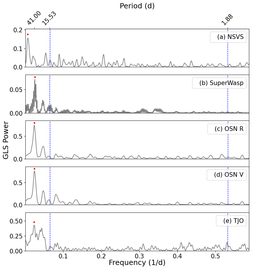
Figure 10: GLS periodograms of the long-term photometry data from NSVS, SuperWASP, OSN $R$, OSN $V$, and TJO ($a$–$e$, from top to bottom). Red dots indicate the most significant periods seen in each data set, and vertical dashed blue lines indicate the planet orbital periods of 1.88 d and 15.53 d.

5.1.2 Long-term photometry

To detect periodically modulated signals attributed to rotating surface manifestations of stellar magnetic activity such as dark spots and bright faculae, we examined archival time-series photometry from the All-Sky Automated Survey for Supernovae (ASAS-SN; Shappee et al., 2014), Northern Sky Variability Survey (NSVS; Woźniak et al., 2004), Catalina Sky Survey (Drake et al., 2009), and Wide Angle Search for Planets (WASP; Butters et al., 2010), in a similar fashion as Díez Alonso et al. (2019). In addition, we carried out follow-up photometry with the T150 telescope located at the Observatorio de Sierra Nevada (OSN) in Granada, and the Telescopi Joan Oró (TJO) at the Observatori Astronòmic del Montsec in Lleida, both in Spain. Since the data quality for the ASAS-SN and the Catalina survey was poor, we did not make use of these observations in our analyses. The instrumental setups, as well as the compiled data sets, are described below. We present the observation log in Table 4.

NSVS monitored approximately 14 million objects primarily in the northern hemisphere with $V$ magnitudes ranging from 8.0 mag to 15.5 mag. The main objective was a prompt response to gamma ray burst triggers from satellites to measure the early light curves of their optical counterparts. The robotic telescope array located in Los Alamos, NM, USA, consisted of four unfiltered telephoto lenses and covered a total field of view of $16\times 16$ deg². The photometric data of TOI-1468 were collected between July 1999 and February 2000, and encompass 267 measurements. Details on the basic characteristics and the reduction of the data set were provided by Woźniak et al. (2004).

SuperWASP-North is located in La Palma, Spain, and continuously monitors the sky for planetary transit events (Butters et al., 2010). It consists of eight lenses with a $2048\times 2048$ CCD with pixel sizes of $13.5\,\mu$m, resulting in a field of view of $7.8\times 7.8$ deg² per camera. The observations were conducted with a broadband filter with a passband from 400 nm to 700 nm. The data set for TOI-1468 used in this work were provided by the SuperWASP consortium via the NASA Exoplanet Archive and consists of 34 109 measurements with a baseline of ten years.

T150 is a 150-centimeter Ritchey-Chrétien telescope equipped with a 2k $\times$ 2k Andor Ikon-L DZ936N-BEX2-DD CCD camera with a field of view of 7.9$\,\times\,$7.9 arcmin² (Quirrenbach et al., 2022). The photometric observations were carried out in Johnson $V$ and $R$ filters, covering 52 epochs between September 2020 and January 2021, with typical exposure times of 70 s in $V$ and 40 s in $R$. All CCD measurements were obtained by the method of synthetic aperture photometry using a 2 $\times$ 2 binning. Each CCD frame was corrected in a standard way for bias and flat fielding. Different aperture sizes were tested to find the optimal one for our observations. After removing $3\sigma$ outliers due to bad weather conditions, the rms on each night was about 3.0 mmag and 2.5 mmag in $V$ and $R$ bands, respectively.

TJO is a 0.8-meter robotic telescope equipped with the 4k $\times$ 4k back-illuminated CCD camera LAIA, which has a pixel scale of 0.4 arcsec and a squared field of view of 30 arcmin². Several blocks of five images were collected between August 2020 and January 2021 over the course of 150 nights using the Johnson $R$ filter. The images were calibrated with bias, darks, and flat fields with the ICAT pipeline (Colome & Ribas, 2006). Differential photometry was extracted with AIJ (Collins et al., 2017), with the aperture size and the set of comparison stars that minimized the rms of the photometry.

Figure 10 shows the most significant signal of the GLS periodograms of the long-term photometry. Almost all data sets show pronounced peaks between 38 d and 41 d, as well as a strong secondary signal at half this range, at $\sim$21 d, which would correspond to the first harmonic. However, other secondary peaks at $\sim 20$ d and $\sim 45$ d also are also present. These periods may be associated with the rotation period of the star, since for old M dwarfs these values are typically in the range of 10 to 150 d (Jeffers et al., 2018). The only exception is the NSVS light curve, which also shows a dominant peak at 147 d (not shown in the diagram), longer than half its time baseline. However, these data are much noisier and shorter than the others, and since the rest of the photometry data and spectroscopic activity indicators share a common periodicity of about $\sim$41 d, we question the reliability of this peak.

Next, we applied a more sophisticated approach and modeled the light curves with a Gaussian process (GP). We used the fitting tool juliet (Espinoza et al., 2019), which incorporates the Python library george (Ambikasaran et al., 2015) for the in-built kernels. For our purpose, we selected the quasi-periodic (QP) kernel, which is an exponential-sine-squared kernel multiplied by a squared-exponential kernel, which allows complex periodic signals to be modeled. This kernel is suitable for accounting for the effects of active regions present on the surface of stars, which often mimic a sinusoidal-like signal (Angus et al., 2018). It has the form:

$$k(\tau)\,=\,\sigma^{2}_{\rm GP}\,\exp\left(-\alpha_{\rm GP}\,\tau^{2}-\Gamma\sin^{2}\left[\frac{\pi\tau}{P_{\rm rot;GP}}\right]\right)\leavevmode\nobreak\ ,\leavevmode\nobreak\$$ (1)

where $\sigma_{\rm GP}$ is the GP amplitude (in parts per million, ppm), $\Gamma$ is the dimensionless amplitude of the GP sine-squared component, $\alpha$ is the inverse length scale of the GP exponential component (d^-2), $\tau$ is the time lag (d), and $P_{\rm rot;GP}$ is the rotational period of the star (d).

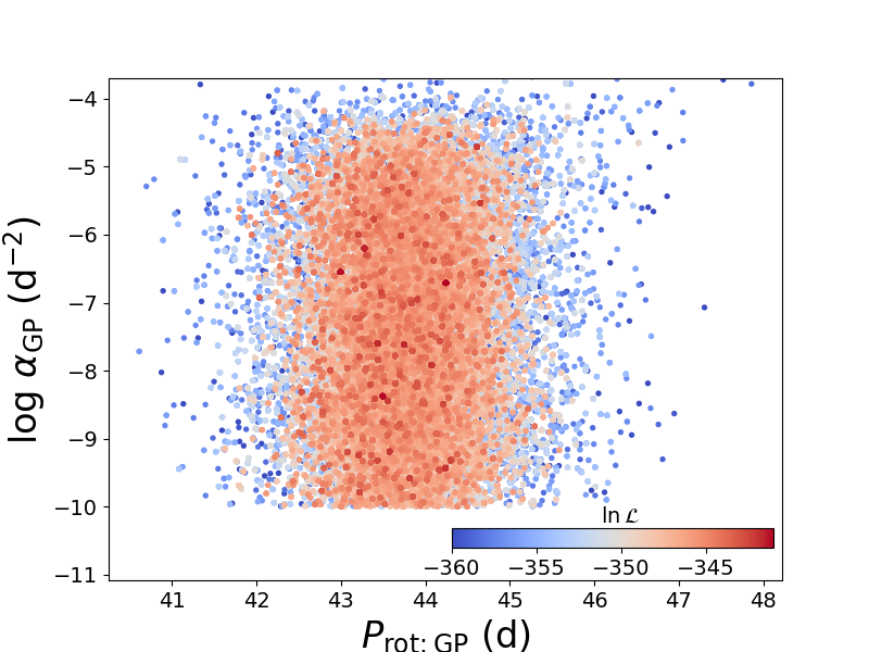
Figure 11: Posterior distribution in the $\alpha_{\rm{GP}}$ vs. $P_{\rm rot;GP}$ plane for the joint GP modeling of NSVS, SuperWASP, OSN $R$, OSN $V$, and TJO photometry data. The normalized log-likelihood increases from blue to red.

All the data sets displayed in Fig. 10 were used for the GP modeling. Considering that the photometry data were collected by different instruments and with different filters, we let the values of $\sigma_{\rm{GP}}$ and $\Gamma$ be variable for each data set and kept the $\alpha$ and $P_{\rm rot;GP,Phot}$ as common parameters. As justified by Stock et al. (2020), wide uninformative priors were used for all parameters: $\sigma_{\rm{GP}}$ (Jeffreys distribution between $10^{-2}$ ppm and $10^{2}$ ppm), $\Gamma$ (Jeffreys distribution between $10^{-6}$ and $10$), instrumental jitter (Jeffreys distribution between 0.01 ppm and $100$ ppm), $\alpha$ (uniform between $10^{-10}$ d^-2 and $10^{-2}$ d^-2), and $P_{\rm rot;GP}$ (uniform between 30 d and 50 d). The relative offset between fluxes of different instruments was chosen to have a normal distribution between 0 and $1000$.

We determined the rotational period from the GP analysis as $P_{\rm rot;GP}$ = $43.8\pm 0.7$ d. We plot the $\alpha_{\rm GP}$ vs $P_{\rm rot;GP}$ diagram in Fig. 11, similar to previously discussed by Stock et al. (2020), Bluhm et al. (2021), and Kossakowski et al. (2021). This diagram gives an idea if a strong correlated noise (small $\alpha$) would favor any periodicity. As seen in Fig. 11, a peak is centered around 44 d with log $\alpha$ values spread between $-4$ to $-10$, which are indicative of the fact that the GP is modeling a periodic signal in the entire $\alpha$ range.

Based on our analysis of the $P_{\rm rot;GP}$ derived by the GP, the photometric GLS periodogram, and spectroscopic activity indicators, we conclude that the rotational period of the star should be around 41–44 d, indicating that TOI-1468 is a slow rotator. Such a long rotation period is consistent with the object being older than the Praesepe open cluster (Curtis et al., 2019), whose age ranges from 590 Ma to 900 Ma (Delorme et al., 2011; Lodieu et al., 2019).

5.2 Orbital fits of the TOI-1468 planets

To determine the orbital elements of the TOI-1468 system, we used the Python-based library juliet and modeled the transit data, the RV data, as well as both data sets in a joint manner. The juliet library makes use of other Python packages: radvel (Fulton et al., 2018) for RV modeling, and batman (Kreidberg, 2015) for transit modeling. Based on the initial supplied prior inputs, juliet uses dynamic nested sampling from dynesty (Speagle, 2020) to compute the Bayesian model log evidence, $\ln\mathcal{Z}$, along with posterior samples. There is a provision to model GPs that are implemented through george (Ambikasaran et al., 2015) and celerite (Foreman-Mackey et al., 2017).

Table 5: Posterior parameters of the joint fit for TOI-1468 b and c.

Parametera	TOI-1468 b	TOI-1468 c
$P$ (d)	$1.8805136^{+0.0000024}_{-0.0000026}$	$15.532482^{+0.000034}_{-0.000033}$
$t_{0}$ (BJD)	$2458765.68079^{+0.00070}_{-0.00069}$	$2458766.9269^{+0.0012}_{-0.0012}$
$a/R_{\star}$	$13.14^{+0.21}_{-0.24}$	$53.69^{+0.84}_{-0.97}$
$b\,=\,(a/R_{\star})\cos i_{\rm p}$	$0.350^{+0.062}_{-0.075}$	$0.623^{+0.023}_{-0.024}$
$i_{\rm p}$ (deg)	$88.47^{+0.34}_{-0.29}$	$89.335^{+0.032}_{-0.035}$
$r_{1}$	$0.567^{+0.041}_{-0.050}$	$0.749^{+0.015}_{-0.016}$
$r_{2}$	$0.0341^{+0.0009}_{-0.0009}$	$0.055^{+0.0008}_{-0.0009}$
$K$ ($\mathrm{m\,s^{-1}}$)	$3.40^{+0.25}_{-0.24}$	$3.48^{+0.34}_{-0.35}$
Derived physical parameters
$M\,(M\oplus)$	$3.21^{+0.24}_{-0.24}$	$6.64^{+0.67}_{-0.68}$
$R\,(R\oplus)$	$1.280^{+0.038}_{-0.039}$	$2.064^{+0.044}_{-0.044}$
$g\,(\rm{m\,s^{-2}})$	$19.12^{+1.93}_{-1.76}$	$15.26^{+1.68}_{-1.63}$
$S\,({S\oplus})$	$36.0^{+1.6}_{-1.4}$	$2.15^{+0.09}_{-0.09}$
$T_{\rm eq}\,\rm(K)^{b}$	$682.2^{+7.4}_{-6.9}$	$337.5^{+3.7}_{-3.4}$

Table 6: Posterior distributions of the juliet joint fit for the instrumental and GP fit parameters obtained for the TOI-1468 system.

Parametera	TOI-1468
Stellar parameters
$\rho_{\star}$ ($\mathrm{g\,cm\,^{-3}}$)	$12.13^{+0.58}_{-0.65}$
Photometry parameters
$M_{\mathrm{TESS\,17}}$ ($10^{-6}$)	$-72^{+25}_{-27}$
$\sigma_{\mathrm{TESS\,17}}$ (ppm)	$0.29^{+6.42}_{-0.25}$
$q_{1,\mathrm{TESS\,17}}$	$0.70^{+0.19}_{-0.23}$
$q_{2,\mathrm{TESS\,17}}$	$0.57^{+0.26}_{-0.29}$
$M_{\mathrm{TESS\,42}}$ ($10^{-6}$)	$-64^{+15}_{-16}$
$\sigma_{\mathrm{TESS\,42}}$ (ppm)	$0.39^{+13.73}_{-0.38}$
$q_{1,\mathrm{TESS\,42}}$	$0.086^{+0.126}_{-0.060}$
$q_{2,\mathrm{TESS\,42}}$	$0.39^{+0.35}_{-0.25}$
$M_{\mathrm{TESS\,43}}$ ($10^{-6}$)	$-48^{+14}_{-15}$
$\sigma_{\mathrm{TESS\,43}}$ (ppm)	$0.27^{+10.63}_{-0.26}$
$q_{1,\mathrm{TESS\,43}}$	$0.31^{+0.26}_{-0.18}$
$q_{2,\mathrm{TESS\,43}}$	$0.29^{+0.27}_{-0.19}$
$M_{\mathrm{LCO-SAAO}}$ ($10^{-6}$)	$-74^{+67}_{-67}$
$\sigma_{\mathrm{LCO-SAAO}}$ (ppm)	$1195^{+63}_{-60}$
$q_{1,\mathrm{LCO-SAAO}}$	$0.68^{+0.20}_{-0.30}$
$M_{\mathrm{LCO-SSO}}$ ($10^{-6}$)	$-7^{+76}_{-80}$
$\sigma_{\mathrm{LCO-SSO}}$ (ppm)	$1873^{+64}_{-65}$
$q_{1,\mathrm{LCO-SSO}}$	$0.72^{+0.16}_{-0.22}$
$M_{\mathrm{LCO-MCD}}$ ($10^{-6}$)	$-42^{+50}_{-51}$
$\sigma_{\mathrm{LCO-MCD}}$ (ppm)	$842^{+47}_{-46}$
$q_{1,\mathrm{LCO-MCD}}$	$0.58^{+0.17}_{-0.19}$
$M_{\mathrm{MUSCAT2}}$ ($10^{-6}$)	$-610^{+120}_{-120}$
$\sigma_{\mathrm{MUSCAT2}}$ (ppm)	$0.57^{+19.58}_{-0.56}$
$q_{1,\mathrm{MUSCAT2}}$	$0.40^{+0.28}_{-0.25}$
$M_{\mathrm{KUIPER}}$ ($10^{-6}$)	$-670^{+190}_{-190}$
$\sigma_{\mathrm{KUIPER}}$ (ppm)	$1.9^{+187.0}_{-1.9}$
$q_{1,\mathrm{KUIPER}}$	$0.74^{+0.17}_{-0.27}$
RV parameters
$\mu_{\mathrm{CARMENES}}$ ($\mathrm{m\,s^{-1}}$)	$-0.14^{+4.14}_{-4.31}$
$\sigma_{\mathrm{CARMENES}}$ ($\mathrm{m\,s^{-1}}$)	$1.553^{+0.384}_{-0.399}$
$\mu_{\mathrm{MAROON-X,Blue,1}}$ ($\mathrm{m\,s^{-1}}$)	$-0.54^{+4.14}_{-4.39}$
$\sigma_{\mathrm{MAROON-X,Blue,1}}$ ($\mathrm{m\,s^{-1}}$)	$0.425^{+1.102}_{-0.379}$
$\mu_{\mathrm{MAROON-X,Blue,2}}$ ($\mathrm{m\,s^{-1}}$)	$1.93^{+4.12}_{-4.46}$
$\sigma_{\mathrm{MAROON-X,Blue,2}}$ ($\mathrm{m\,s^{-1}}$)	$0.210^{+1.156}_{-0.178}$
$\mu_{\mathrm{MAROON-X,Red,1}}$ ($\mathrm{m\,s^{-1}}$)	$-0.88^{+4.21}_{-4.37}$
$\sigma_{\mathrm{MAROON-X,Red,1}}$ ($\mathrm{m\,s^{-1}}$)	$0.143^{+0.470}_{-0.115}$
$\mu_{\mathrm{MAROON-X,Red,2}}$ ($\mathrm{m\,s^{-1}}$)	$1.01^{+4.22}_{-4.55}$
$\sigma_{\mathrm{MAROON-X,Red,2}}$ ($\mathrm{m\,s^{-1}}$)	$1.731^{+1.104}_{-0.850}$
GP hyperparameters
$\sigma_{\mathrm{GP,RV}}$ ($\mathrm{m\,s^{-1}}$)	$6.602^{+5.56}_{-2.89}$
$\alpha_{\mathrm{GP,RV}}$ ($10^{-6}\,\mathrm{d^{-2}}$)	$0.17^{+252}_{-0.16}$
$\Gamma_{\mathrm{GP,RV}}$	$0.33^{+0.76}_{-0.17}$
$P_{\mathrm{rot;GP,RV}}$ (d)	$41.48^{+0.16}_{-0.17}$

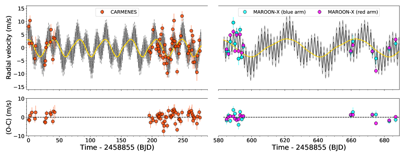
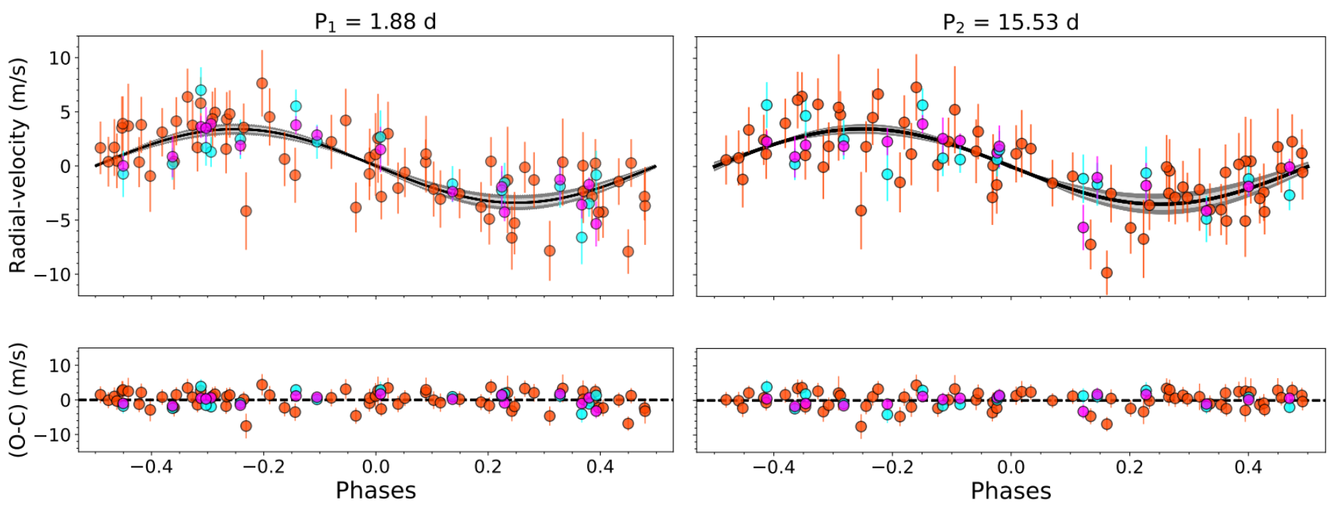
Figure 12: Joint modeling of the RV data from CARMENES (VIS: orange), MAROON-X (Blue arm: cyan; Red arm: magenta) for TOI-1468, along with their residuals. In both panels, the solid curve is the median best-fit juliet model. The light and dark gray shaded regions represent $68\,\%$ and $95\,\%$ credibility bands, respectively. Top panel: RV time-series with the GP component (solid yellow curve). Bottom panel: Phase-folded RVs for TOI-1468 for the inner 1.88 d-period planet and the outer 15.53 d-period planet, along with their residuals folded at their respective periods.

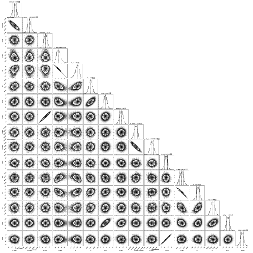
Figure 18: Posterior distribution for the joint model parameters (2cp+GP) derived with juliet.

Mutually independent parameters were constrained through transit-only and RV-only fits with juliet (see Appendix A for details). More precise values of $P$, $T_{c}$, $\omega$, and $e$ were obtained by performing a simultaneous fit to all parameters. For the purpose of joint fitting, we used the RV points from CARMENES and MAROON-X, the light curves from TESS, and ground-based photometry. The best-fit results from the transit-only and the RV-only analyses were used as priors. The 2cp+GP model was chosen for modeling the RV points, as discussed in A.2. The complete list of priors used for the joint fit are described in Table 8. The RV semi-amplitude, $K$ value for the inner planet is $3.403^{+0.246}_{-0.244}$ m $\rm s^{-1}$, and the $K$ value for the outer planet is $3.485^{+0.344}_{-0.351}$ m $\rm s^{-1}$. The posterior planet parameters for the joint orbital fit are presented in Table 5 and in Table 6. The covariance plot for the fitted parameters is presented in Fig. 18. However, uncertainties in planet mass and radius depend on the input uncertainties in stellar mass, radius, and equilibrium temperature, which in this case may be underestimated. As a result, the actual planet densities of TOI-1468 b and c may differ by more than $1\sigma$ from the values derived by us, and a better characterization of the planet-host star would be desirable. See Caballero et al. (2022) for an exhaustive analysis on sources of error and propagation of uncertainty of parameters of transiting planets with RV follow-up.

As described by the posterior parameters of our joint fit, and the resulting RV model presented in Fig. 12, the maximum posteriori of the GP periodic component, $P_{\mathrm{rot,GP:RV}}$, is about 41 d, which is in agreement with the signal observed in the GLS periodogram of the RVs (Fig. 8) and corresponds to the stellar rotation period. The best-fit results obtained from joint modeling are displayed in Figs. 4 and 5 for transits, and Fig. 12 for RVs.

6 Discussion

6.1 The radius valley

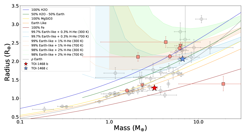
Figure 13: Mass-radius diagram of well-characterized planets with radii $R<3\,R_{\oplus}$ and masses $M<10\,M_{\oplus}$. All the planets plotted in gray are planets transiting M dwarfs taken from Trifonov et al. (2021), last updated on 08 April 2021, with $\Delta M<20\,\%$ and $\Delta R<20\,\%$. The “$\rho$ Earth” is the constant Earth-density line. TOI-1468 b and c are marked with red and blue stars, respectively, and LTT3780 b;c, L231-32 b;c;d, and TOI1749 b;c;d are marked with salmon filled circles, inverted triangles and squares, respectively. Theoretical mass-radius relations are taken from Zeng et al. (2019).

We plot all the planets transiting M dwarfs determined with a precision of better than $20\%$ for masses and radii in Fig. 13. We used the transiting M dwarfs as listed by Trifonov et al. (2021), updated on 08 April 2021. The compositional models from (Zeng et al., 2019) are also shown. TOI-1468 b and c are marked with red and blue stars, respectively. The inner planet has a bulk density consistent with a composition ranging from $50\%$ silicates and $50\%$ iron, to $100\%$ silicates. The planet appears to have been irradiated, which is indicative of atmospheric losses. The mass and radius for TOI-1468 c indicates that it must have a low-density envelope. As the losses depend on the amount of XUV radiation that the planet receives, the evolution of the two planets orbiting the same star at different distances can be different. For example, the inner one may lose the H/He envelope, while the outer one keeps it. When XUV erosion is considered as a possible explanation for the radius valley, the valley must depend on the orbital separation of the host star and also its spectral type (FGK or M), with the same planetary composition. There have been a handful of discoveries for systems with multiple planets straddling the radius valley around different spectral type stars: K2-36 b c (Damasso et al., 2019), K2-106 b, c (Guenther et al., 2017), HD3167 b, c (Gandolfi et al., 2017), GJ9827 b, c, d (Niraula et al., 2017), or Kepler10 b, c (Dumusque et al., 2014), to name a few. There are only a few such examples for planets on the opposite sides of the radius valley for transiting M dwarfs, such as LTT3780 b, c (Nowak et al., 2020; Cloutier et al., 2020), L231-32 b, c, d (Van Eylen et al., 2021), and TOI1749 b, c, d (Fukui et al., 2021). A common observation governing all the discoveries is the fact that, in most of these systems, the inner planet has a rocky Earth-like composition, and the outer planet or planets have solid cores with an outer envelope composed of lighter gases such as H and He.

It was also demonstrated by Van Eylen et al. (2018) that this radius valley narrows for smaller orbital periods. Both these observations are consistent with the photoevaporation model, although it cannot be excluded that it is due to formation. Core-powered mass loss (Ginzburg et al., 2018; Gupta & Schlichting, 2020) has been suggested as an alternate hypothesis for the origin of the radius valley. There are also suggestions of different formation mechanisms for the planets on both sides of the radius valley, where one side of the valley consists of water-worlds, and the other consists of rocky and terrestrial planets (Zeng et al., 2019). It is imperative to find out if the radius valley is lower for M stars than for FGK stars, this system being an important contribution. This would imply a strong argument for the atmospheric erosion via XUV radiation. A core-powered model would be able to explain this, if it is assumed that the ratio of rocky to icy planets is different for M stars than for FGK stars. It is interesting to focus on multi-planet systems on two sides of the radius valley, which could be the key to answering similar questions. For example, the evolution of a planet orbiting a young active star should be different from a planet orbiting a young but inactive star. Measurements of the isotope ratios $\rm{}^{36}Ar/^{38}Ar$, $\rm{}^{20}Ne/^{22}Ne$, and $\rm{}^{36}Ar/^{22}Ne$ on Earth and Venus, and the abundances of sodium and potassium of the lunar regolith both indicate that our Sun was only weakly active in the first 100 Ma (Lammer et al., 2019). Thus, the evolution of the planets in our Solar-System could quite be different from those orbiting M stars that were very active when they were young and also stayed in this high-activity phase for a long time. For this reason, it is important to study the properties of low-mass planets orbiting particularly low-mass stars.

6.2 System architecture

The scaled orbital separation ($a/R_{\star}$) for the inner planet, TOI-1468 b, is $13.139^{+0.205}_{-0.238}$. The light curves from TESS and the several ground-based transit measurements taken for the inner planet results in $R_{\rm b}$ as $1.280^{+0.038}_{-0.039}\,R_{\oplus}$. The mass for the planet, as derived by the RV measurements from CARMENES, is $M_{\rm b}$ = $3.21\pm 0.24\,M_{\oplus}$. This gives us the bulk planet density as $\rho_{\rm b}$ = $8.39^{+1.05}_{-0.92}$ g cm^-3. The total amount of insolation received by the inner planet is 36 times that of Earth. Assuming a zero albedo and a uniform dayside temperature, the equilibrium temperature of TOI-1468 b is $\sim$682 K.

Similarly, the scaled orbital separation for the outer planet, TOI-1468 c, is $53.687^{+0.839}_{-0.975}$. The radius and mass for the planet are $2.06\pm 0.04$ $R_{\oplus}$ and  $6.64^{+0.67}_{-0.68}\,M_{\oplus}$, respectively. This results in a bulk planet density of $\rho_{\rm c}$ = $2.00^{+0.21}_{-0.19}$ g cm^-3. The stellar insolation for the outer planet TOI-1468 c is twice that of the Earth and, with a zero albedo, has an equilibrium temperature of $\sim$337 K. Apparently TOI-1468 c could be located close to the inner edge of of the habitable zone (Kasting et al., 1993; Kasting, 1998, 2010; Kasting & Harman, 2013; Kopparapu et al., 2014; Kasting, 2021), and probably the actual temperature should be much higher than the equilibrium temperature, due to atmospheric heating effects. However, since the planet is most likely tidally locked, this does not exclude the possibility of surface liquid water (e.g., Wandel, 2018; Martínez-Rodríguez et al., 2019).

Systems similar to the TOI-1468 system are interesting from the point of view of planet formation: two planets that orbit the same host star on close-in orbits but have different densities. It could be that both these planets formed in different environments. It is possible that TOI-1468 b formed at its current location, whereas TOI-1468 c could have formed further out and eventually migrated in (Ida & Lin, 2010). The other explanation is that both planets could have formed in similar environments, but the photoevaporation due to the XUV radiation could have stripped off a substantial portion of the inner planet’s gaseous envelope due to hydrodynamic losses (López & Fortney, 2013). The mass loss history of planets depends on the amount of incident radiation they receive from the host star and the mass of the planet core. The critical mass loss timescale (López & Fortney, 2013) for TOI-1468 b is $\sim$ 2.5 Ga, which is on the order of the age of the star, and the critical mass loss timescale for the outer planet is twenty times larger, which suggests the survival of the outer atmosphere. This theory is also supported by the fact that there are no low-density exoplanets found in close-in orbits to their host stars where they would face extreme irradiation (Lopez et al., 2012). Moreover, in many multi-planet systems it is commonly observed that inner planets are smaller than the outer planet, which can be better explained by a photoevaporation model (Ciardi et al., 2013).

As discussed by Cubillos et al. (2017) and Guenther et al. (2017), another useful parameter to look at is the thermal escape for a hydrodynamic atmosphere subjected to the gravitational perturbation from the host star in terms of the restricted Jeans escape rate (Fossati et al., 2017),

$$\Lambda\,=\,\frac{GM_{p}m_{\rm H}}{k_{\rm b}T_{\rm eq}R_{p}}\leavevmode\nobreak\ ,\leavevmode\nobreak\$$ (2)

where $\Lambda$ is the Jeans escape parameter for a hydrogen atom with mass ($m_{\rm H}$) evaluated at the planet with its mass ($M_{\rm p}$), radius ($R_{\rm p}$), and equilibrium temperature ($T_{\rm eq}$). $G$ and $k_{\rm b}$ are the gravitational and Boltzmann constants, respectively. The value of $\Lambda$ gives an understanding on the stability of the planetary atmosphere against evaporation. In the case of TOI-1468, $\Lambda$ is $\sim 29$ for the inner planet and $\sim 80$ for the outer one. This result puts the inner planet in the $\Lambda$ regime of 20–40, which is typical for the boil-off regime planets (Owen & Wu, 2016) where the atmosphere escape is driven by the thermal energy and low planetary gravity. Systems such as TOI-1468 are excellent test beds to study planets that straddle the radius valley, offering further insights into their formation mechanisms.

6.3 Additional planet candidates

In a study by Dietrich & Apai (2020), a model was created with population statistics to predict previously undetected planets in the existing multi-planetary TESS systems. Their model predicted TOI-1468 to have an additional planet at an orbital period of $3.82^{+0.93}_{-0.75}$ d with a planet radius of $1.63^{+0.57}_{-0.42}$ $R_{\oplus}$, whereas the clustered periods model predicted an orbital period of $2.68^{+0.15}_{-0.01}$ d with a planet radius of $1.63^{+0.57}_{-0.42}\,R_{\oplus}$ for the additional planet. We decided to apply the box least-square (BLS; Kovács et al., 2002) algorithm to the PDCSAP TESS light curves to search for additional transits. After removing the two transiting planets, there was no indication of any significant signal in the data corresponding to a planet with an upper limit of $\sim 1.0$ $R_{\oplus}$ in the similar period range.

Since we did not find any further statistically significant signals, except the known transit signals, in the data set, this hints that the hypothetical planet either does not exist, or would be likely non-transiting. Since the predicted planet should have an orbital period that covers the 2:1 period commensurability with the known inner planet, we searched the TESS and ground-based light curves for transit timing variations (TTVs). We did not detect any significant hints for TTVs (Fig. 14). We note that, depending on the period of the hypothetical planet, the TTV period would be longer than the baseline covered by the observations ($\sim$ 750 d) and that the S/N was so far not sufficient to detect variations in the minute range. We also did not find any evidence of this planet in our RV data.

Planet formation models of core accretion predict an enhanced giant planet occurrence in systems with high-density rocky planets (Schlecker et al., 2021). The different bulk densities of TOI-1468 b and c do not allow a clear prediction in this regard. However, the possible high abundance of volatiles in TOI-1468 c allows us to make the assumption that no gas giant is present in the system, which would have prevented the transport of volatile-rich material into the inner system. No such planet is expected from simulated systems with host stars with masses similar to that of TOI-1468 (Burn et al., 2021), and we do not observe evidence for an outer giant planet companion.

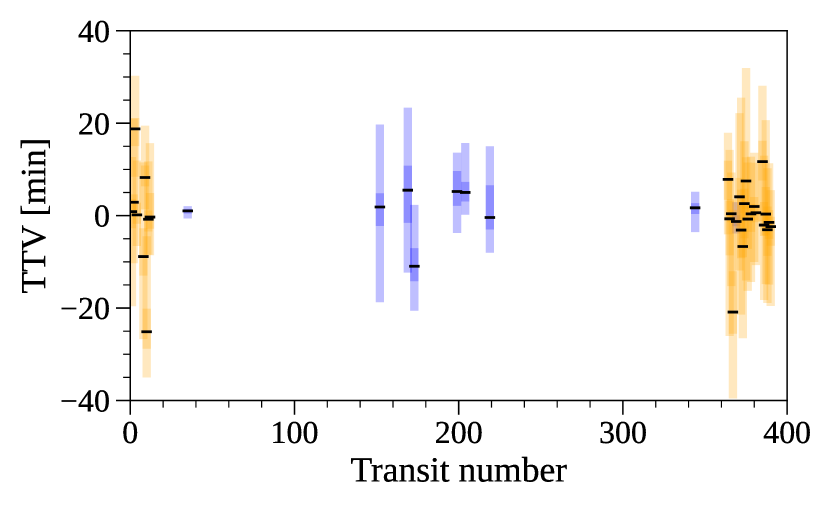
Figure 14: TOI-1468 b transit-timing variations from TESS data (orange) and follow-up observations (blue). The different shades of color of the error bars represent the 1$\sigma$ (dark) and 3$\sigma$ (light) levels of uncertainty of the measurements. No significant TTVs are detected in the $\sim 750$ d of baseline covered by the observations.

6.4 Atmospheric characterization

Multi-planet systems provide additional opportunities for atmospheric characterization. Satellite missions such as the James Webb Space Telescope (JWST) or the upcoming Atmospheric Remote-sensing Infrared Exoplanet Large-survey (ARIEL) (Tinetti et al., 2016) offer excellent space-based laboratories for such studies. To qualitatively assess the suitability of both planets for atmospheric investigations, we calculated the transmission spectroscopy metrics (TSMs) and emission spectroscopy metrics (ESMs), as defined by Kempton et al. (2018). We generated 10⁵ random extractions of the planetary, orbital, and stellar parameters according to their error bars, thus obtaining the probability density function for each TSM and ESM factor. For the inner planet, we obtained $\mathrm{TSM}_{\mathrm{b}}=9\pm 1$ and $\mathrm{ESM}_{\mathrm{b}}=6.3_{-0.6}^{+0.8}$. Both values are close to the recommended thresholds of ten and 7.5, respectively, defining the top-ranked atmospheric targets in the terrestrial sample. The outer planet is a small sub-Neptune with $\mathrm{TSM}_{\mathrm{c}}=59_{-10}^{+12}$, $90$ being the threshold for its category. It is worth noticing that these metrics rank the planets based solely on the predicted strength of an atmospheric detection. Having TSM and/or ESM values slightly below the threshold does not indicate that detailed atmospheric studies are impossible or challenging with current facilities. In other words, these metrics are not the unique criteria for determining the best targets for atmospheric studies. Scientific interest can also inspire observing proposals, for example the opportunity to explore a system with small temperate planets straddling the radius valley around an M dwarf.

To quantitatively assess the potential for atmospheric characterization of both planets, we generated synthetic JWST spectra for a range of atmospheric scenarios. Our simulations made use of the photo-chemical model ChemKM (Molaverdikhani et al., 2019b, a, 2020), the radiative transfer code petitRADTRANS (Mollière et al., 2019), and ExoTETHyS (Morello et al., 2021) to incorporate the overall response of the JWST system, including realistic noise and error bar estimates. For each planet, we considered a benchmark model with H/He gaseous envelope and solar abundances, and other two models showing the effect of haze or enhanced metallicity (100$\times$ solar abundances).

The transmission spectra for the H/He-dominated atmospheres show strong absorption features due to H₂O and CH₄ over the wavelength range 0.5–12 $\mu$m (see Fig. 15). The spectroscopic modulations are on the order of 400–600 ppm and 100–200 ppm for TOI-1468 b and c, respectively, with a relatively modest dampening effect due to haze or metallicity, particularly at shorter wavelengths. Similar trends with enhanced metallicity or haze were also observed in simulations made for other planets (e.g., Nowak et al., 2020; Trifonov et al., 2021; Espinoza et al., 2022), but the features are essentially muted in the cases with 100$\times$ solar metallicity and haze (not shown here).

We simulated JWST spectra for the NIRISS/SOSS (0.6–2.8 $\mu$m), NIRSpec/G395M (2.88–5.20 $\mu$m), and MIRI-LRS (5–12 $\mu$m) instrumental modes. The wavelength bins were specifically determined, through ExoTETHyS, to have similar counts, leading to nearly uniform error bars per spectral point. We also used PandExo (Batalha et al., 2017) to check the best setups for each instrumental mode and the corresponding observing efficiencies (i.e., the fraction of effective integration time per given observing interval). Finally, we inflated the error bars by a factor of 1.2 to account for correlated noise. In particular, the spectral error bars estimated for just one transit observation per instrument configuration are 40-60 ppm at wavelengths $<$5 $\mu$m, with a median resolving power $R\sim 50$ and 75-100 ppm at wavelengths $>$5 $\mu$m with bin sizes of $\sim$0.1–0.2 $\mu$m. The lower error bars are estimated for the outer planet owing to its longer transit duration. Based on these numbers and the visualization of the simulated spectra in Fig. 15, we conclude that a single transit observation in any of these JWST modes would be sufficient for robust detection of the molecular features in the H/He-dominated scenarios, and the larger wavelength coverage provided by the three modes can help distinguish between the effects of metallicity and haze. However, the possible lack of a H/He envelope around the inner planet would represent a challenge for detecting its atmosphere, if any, even with JWST, unless many observations are stacked together.

Even if TOI-1468 b may have lost its primordial atmosphere, resupply of H can occur under favorable circumstances. A possible mechanism consists in the dissolution of H/He in the magma ocean of young planets and subsequent outgassing that can recreate a substantial atmosphere (Chachan & Stevenson, 2018; Kite et al., 2019; Kite & Barnett, 2020). Recently, this scenario has been proposed to explain the tentative detection of the HCN absorption feature on the terrestrial planet GJ 1132 b (Swain et al., 2021), although the authenticity of the spectral feature has been debated (Mugnai et al., 2021). Tentative evidence of H₂O vapor in a H/He envelope has been reported for the habitable-zone super-Earth LHS 1140 b (Edwards et al., 2021), which, similar to GJ 1132 b and TOI-1468 b, belongs to the left side (at the very edge) of the radius valley.

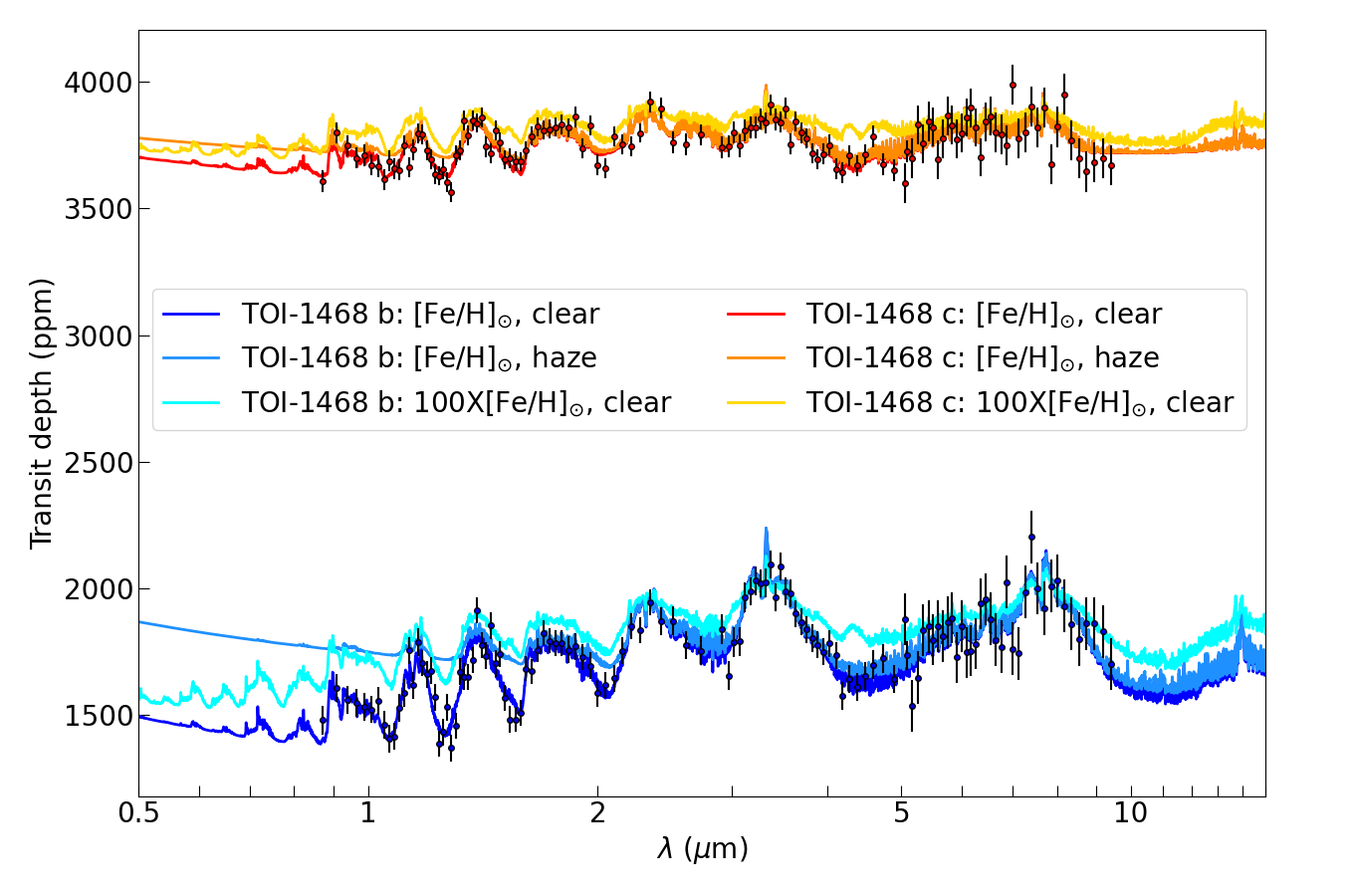
Figure 15: Synthetic JWST transmission atmospheric spectra of TOI-1468 b and c. Fiducial models with solar abundances and no haze (solid blue and red lines), with haze (dodger blue and orange), and enhanced metallicity by a factor of 100 (cyan and gold). Estimated uncertainties are shown for the simulated observation of one transit with JWST NIRISS-SOSS, NIRSpec-G395M, and MIRI-LRS configurations.

7 Summary

The TOI-1468 system consists of an early-to-mid-type M dwarf (LSPM J0106+1913) with two transiting planets in circular orbits. The host star has a surface temperature of $T_{\rm eff}=3496\pm 25$ K, surface gravity of $\log{g}=5.00\pm 0.11$ dex, and a metallicity of [Fe/H] = $-0.04\pm 0.07$ dex. We thereby determine a stellar mass of $0.339\pm 0.011\,M_{\odot}$ and a stellar radius of $0.344\pm 0.005$ $R_{\odot}$. The relatively bright star ($G$ = 12.10 mag, $J$ = 9.34 mag) is located at a distance of $24.72\pm 0.02$ pc and has a high proper motion of $332$ mas a^-1. We also determine that the star is inactive with a relatively long rotational period of around 41–44 d.

This multi-planet system consists of an inner super-Earth having a mass of $M_{\rm b}$ = $3.21\pm 0.24$ $M_{\oplus}$ and a radius of $R_{\rm b}=1.280^{+0.038}_{-0.039}\,R_{\oplus}$, with an orbital period of 1.88 d, and an outer planet with a mass of $M_{\rm c}$ = $6.64^{+0.67}_{-0.68}$ $M_{\oplus}$ and a radius of $R_{\rm c}$ = $2.06\pm 0.04$ $R_{\oplus}$, with an orbital period of 15.53 d, and is therefore close to the inner edge of the habitable zone. The bulk densities of the inner and outer planets are $8.39^{+1.05}_{-0.92}$ g cm^-3 and $2.00^{+0.21}_{-0.19}$ g cm^-3, respectively. Multi-planet systems with planets lying on opposite sides of the radius valley are interesting laboratories to probe planet formation models through atmospheric studies. For example, according to the photoevaporation theory, the atmosphere of the outer planet is likely to be primordial metal enriched, while the inner one may host a secondary atmosphere, or none. Thus, accurate measurements of planetary masses and radii, such as those presented in this work, are required in order to estimate their density and determine the extent to which their atmosphere has been retained or removed. Finally, spectroscopic observations of just a few transits and eclipses of TOI-1468 b and c with the JWST would provide an excellent opportunity to test photoevaporation, as well as other formation and evolution scenarios.

Appendix A Data modeling with juliet

A.1 Transit-only modeling

We fit the TESS light curve from sectors 17, 42, and 43 to determine more precise transit parameters using the SPOC reported period and ephemeris for each planet. We used this information as initial input parameters to precisely determine the ephemeris of the transiting planets. As a first step, we allowed the period of the inner planet to vary between 1.6 and 2.1 days, whereas, for the outer planet we kept this range between 15.2 and 15.8 days. We also incorporated the central transit time for both the planets based on the TESS light curves, analyzed with the SPOC pipelines (Jenkins et al. 2016), namely between BJD 2458765.5 and 2458765.8 for the inner planet, and between 2458766.7 and 2458767.1 for the outer planet. The transit fitting is usually done by fitting the scaled planetary radius, $a/R_{\star}$, as a free parameter. Since we have a multiple planet system, we instead fitted the stellar density $\rho_{\star},$ introduced first by Sozzetti et al. (2007), which should remain the same for the case of both transiting planets and constrain it in a more robust way. We kept $\rho_{\star}$ as a free parameter with a normal distribution centered around the stellar density and a width of $3\sigma,$ calculated based on stellar parameters as derived in Table 3. Based on Espinoza (2018), we also parametrized the planet-to-star-ratios, $p_{\rm 1}$, $p_{\rm 2}$, and the impact parameters, $b_{\rm 1}$, $b_{\rm 2}$ to fit variables $r_{\rm 1,b}$, $r_{\rm 2,b}$, and $r_{\rm 1,c}$, $r_{\rm 2,c}$ respectively for both planets, and set the priors between 0.0 and 1.0 with a uniform distribution. The RVs provide more information in constraining the eccentricity-omega (e – $\omega$) parameters, and thus these are kept fixed at 0^∘ and 90^∘, respectively, for the transit-only fit. We kept the dilution factor for the TESS and the ground-based photometry fixed at 1.0 as discussed previously in Section 2.2. We also chose a quadratic limb darkening law for the TESS data (Kipping 2013) with a uniform distribution between 0.0 and 1.0. We used a linear limb darkening law for the ground-based data due to relatively low photometric precision, but with the same priors as those for the TESS data. A flux offset was assumed between different photometry data sets, which was allowed to vary between 0.0 and 0.1, and a flux scatter was assumed between $10^{-5}$ to $10^{5}$ ppm, both with a Jeffreys distribution. We recovered the TESS derived periods, $P_{\rm b}$ and $P_{\rm c}$ to be $1.8805175^{+0.0000029}_{-0.0000030}$ d and $15.532244^{+0.000037}_{-0.000046}$ d, and the central transit times, $t_{0b}$, $t_{0c}$ to be $2458765.67857^{+0.00084}_{-0.00082}$ and $2458766.9241^{+0.00050}_{-0.00048}$ (both in BJD), respectively. These initial values with a $3\sigma$ prior width were applied as priors for the joint fit, which is described in 5.2.

A.2 RV-only modeling

Table 7: Comparison of RV-only models.

Models	$\ln{\mathcal{Z}}$	$|\Delta\ln{\mathcal{Z}}|$
Two-signal models (without activity modeling)
2cp	–267.66	0.0
1cp + 1kp	–269.54	1.88
1kp + 1cp	–269.44	1.78
2kp	–271.40	3.74
Three-signal models (with activity modeling)
2cp + sin	–250.44	17.22
2cp + GP	–253.81	13.85
1cp +1kp+ GP	–255.10	12.56
1kp +1cp+ GP	–255.21	12.45
2kp + GP	–256.97	10.69

As discussed in 5.1.1, the CARMENES and MAROON-X RVs show the two transiting planet signals in the GLS periodogram at 1.88 d (and a 2.12 d alias due to the 1 d sampling) and 15.53 d, which both have a nominal false alarm probability (FAP) ¡ 1%. After subtracting the two planetary signals, another signal is seen close to $\sim$41 d (FAP ¡ 0.1%) in the residual periodogram, which is related to the stellar rotation period (see Sect. 5.1).

To find the best model to reproduce our RV data, we performed an extensive model comparison. To select the final model, we used the criteria described in Trotta (2008), which consider a difference between models of $|\Delta\ln\mathcal{Z}|>5$ as “significant”. In this case, the model with the larger Bayesian log evidence is favored. In the case where $|\Delta\ln\mathcal{Z}|>2.5,$ the models are “moderately” favored one over the other. However, if $|\Delta\ln\mathcal{Z}|\leq 2.5$, then the two models are considered “indistinguishable” and a simpler model would be chosen. An overview of the different models and their Bayesian evidence is shown in Table 7. The residual periodogram for our selected model is shown in Fig. 8 (panel d).

Since both planets are statistically significant, we started simultaneously fitting both planet signals using circular Keplerian orbits (“2cp” model). For the period and central time priors, we used normal distributions centered in the values determined through the transit fit (Sect. A.1). The RV amplitude had uniform priors between 0 and 10 m s^-1, the offset parameter of CARMENES and MAROON-X was chosen uniformly between $-10$ and $10$ m s^-1, and the stellar jitter was selected with uniform priors between 0.01 and 10 m s^-1. The residual periodogram of this fit is shown in Fig. 8 (panel c).

To include eccentricity in our models, we parameterized it as $\mathcal{S}_{1}$ = $\sqrt{e}\sin\omega$ and $\mathcal{S}_{2}$ = $\sqrt{e}\cos\omega$ with uniform priors between $-1$ and $1$ (Espinoza et al. 2019). We performed models combining Keplerian planet orbits with fixed eccentricity (“cp”) or kept it free (“kp”). Of these models, those that consider eccentric orbits for one of the two signals are indistinguishable, only the 2kp model is moderately favored ($|\Delta$ln Z— = 3.74) compared with the 2cp fit.

To account for the stellar activity, we then investigated whether including the third signal at $\sim$41 d would improve the log-evidence of the fit. In this case, we modeled it using a sinusoid (sin) or a GP. In the first case, we used uniform priors between 30 and 50 d, which correspond to the suspected region for the stellar rotational period. For the GP selection, we used the QP kernel previously defined in Eq. 1. As we discuss in Sec 5.1, GPs were used to model the rotational signal of the star (Angus et al. 2018). The rotation of the star often produces these sinusoidal-like signals (Dumusque et al. 2011; Haywood et al. 2014), which are misinterpreted in the RV data as a planetary signal. Thus we used a GP as a better way to model these complex periodic signals. For the GP parameters, we used uniform priors for the GP amplitude ($\sigma_{\rm{GP,RV}}$) between 0 and 100 m s^-1. The inverse length scale of the external parameter ($\alpha_{\rm{GP,RV}}$) and the amplitude of the sine part of the kernel ($\gamma_{\rm{GP,RV}}$) had a Jeffreys distribution between $10^{-10}$ to $10^{-2}$ and between 0.1 to 10, respectively. The rotational period of the GP ($P_{\rm{rot;GP,RV}}$) had uniform priors between 30 and 50 d. The transiting planets were modeled with both circular and eccentric Keplerians, as done above. These results are summarized in the last five rows of Table 7. Based on the results of the previous table, we noticed that models that include three signals have the largest log-evidence compared with 2cp model. However, the difference between these models are nearly indistinguishable or moderately favored in the case of 2cp + sin ($|\Delta\,\rm ln\,Z|\sim 3.37$). Thus, the first two transiting signals can be best explained with circular planetary orbits, and the third signal close to 41 d can be equally modeled with a sinusoid or a GP fit. However, it is also important to note that the final amplitude and phase of the transiting planets should remain consistent within methods, despite our choice of model for the third signal. In this scenario, given our previous knowledge and having determined that the stellar rotation period should be around 41 – 44 d, and due to the GP allowing us to account for the effects of rotating spots on the data and, therefore, a better way to model the stellar activity, we chose the 2cp+GP as our fiducial model.

A.3 Alternative data modeling with the FCO method

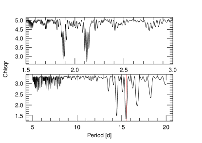
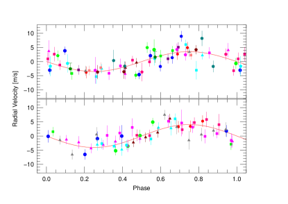
Figure 16: Results from the FCO (“floating chunk offset”) method. Top panels: Periodograms of reduced $\chi^{2}$ for CARMENES RVs as a function of input period for the FCO method for planets TOI-1468 b (top) and c (bottom). Vertical dashed red lines mark the planet orbital periods. Bottom panel: Phase-folded CARMENES RVs for planets TOI-1468 b (top) and c (bottom). Different colors and symbols represent RV values from individual chunks.

We applied an independent alternative method, a “floating chunk offset” (FCO) on CARMENES data to fit the RVs. This method is based on creating an orbital fit to the data by allowing the RV offsets of individual nights to vary with respect to each other (Hatzes et al. 2010; Hatzes 2019). The RV data were divided into 23 chunks, each with 2–4 measurements spanning 2–3 d. For the most part, the chunks used measurements taken on consecutive nights. As a check we performed a FCO periodogram to ensure that FCO was seeing the planet signal (Hatzes et al. 2010; Hatzes 2019). Fig. 16 shows the reduced $\chi^{2}$ as a function of trial periods for the orbital fit. For this periodogram the phase (i.e., transit ephemeris) was allowed to vary so that the best possible fit was made to the data given the trial period. The best fit (minimum $\chi^{2}$) occurs at the transit period of 1.88 d and its alias at 2.14 d. FCO detects the correct signal in the RV data. Applying the FCO method yielded a $K$ amplitude due to planet b of $K_{\rm b}$ = $3.47\pm 0.62$ m s^-1. The lower panel of Fig. 16 shows the final RV variations phased to the orbital period.

To check whether the FCO method was introducing a systematic error into the $K$-amplitude determination, we created a synthetic data set using the orbit of TOI-1468 b with varying $K$-amplitudes. To this we added the orbital motion of TOI-1468 c, a rotational modulation signal with a period of 43 d, and a $K$-amplitude of 2.9 m s^-1. These periodic signals may cause the largest systematic errors because they do not introduce a strictly constant RV value to the chunk. Random noise at a level of 2.3 m s^-1, roughly the rms scatter after removing all signals from the data, was added and the data divided into chunks in the same manner as the observations. The left panel of Fig. 17 shows that the output $K$-amplitude is recovered as a function of the input amplitude over the range 0.5–5.0 m s^-1. The error bars represent the standard deviation of ten simulations, with different realizations of the random noise.

Figure 17: Simulations of the FCO method showing the output $K$ amplitude ($K_{\rm out}$) as a function of the input $K$ amplitude ($K_{\rm in}$) for TOI-1468 b (left) and TOI-1468 c (right).

Finally, we investigated if we could extract the signal of the outer planet. For this, we first removed the contribution of TOI-1468 b from the RV data and created new time chunks so as to sample more of the 15 d period. We used 12 chunks that had time spans ranging from 2 to 7 d, shorter than the 41–44 d region of rotation period. The resulting RV amplitude was $K$ = $4.05\pm 0.59$ m s^-1, which are in excellent agreement with the $K_{\rm b}$ = 3.4 $\pm$ 0.2 m s^-1 determined with the joint fit. The phased RV variations are shown in the bottom panel of Fig. 16. Again, we checked how well FCO could recover known input amplitudes by taking a combination of the orbit of TOI-1468 c combined with the 41–44 d rotation signal. The right panel of Fig. 17 shows that the method recovers the correct amplitude. We indeed see that there is a systematic offset of $+$0.07 m s^-1 between the input and output $K_{\rm c}$-amplitude, most likely due to the residual effects of the 41–44 d period. Applying this offset results in a final RV amplitude of $K_{\rm c}$ = $3.9\pm 0.59$ m s^-1, which is consistent within one sigma with the $K_{\rm c}$ = 3.48 $\pm$ 0.35 m s^-1 previously derived by the joint fit.

Appendix B Long tables

Table 8: Priors used for TOI-1468 b and c in the joint fit with juliet.

Parametera	Prior	Unit	Description
Stellar and planetary parameters
$\rho_{\star}$	$\mathcal{U}(11.0,13.0)$	g cm -3	Stellar density
$P_{\rm b}$	$\mathcal{N}(1.880,0.002)$	d	Period of planet b
$t_{0,b}$	$\mathcal{N}(2458765.681,0.001)$	d	Time of transit center of planet b
$r_{1,b}$	$\mathcal{U}(0,1)$	…	Parameterization for $p$ and $b$
$r_{2,b}$	$\mathcal{U}(0,1)$	…	Parameterization for $p$ and $b$
$K_{b}$	$\mathcal{U}(0,10)$	$\mathrm{m\,s^{-1}}$	RV semi-amplitude of planet b
$e_{b}$	0.0 (fixed)	…	Orbital eccentricity of planet b
$\omega_{b}$	90.0 (fixed)	deg	Periastron angle of planet b
$P_{\rm c}$	$\mathcal{N}(15.538,0.005)$	d	Period of planet c
$t_{0,c}$	$\mathcal{N}(2458766.9236,0.004)$	d	Time of transit center of planet c
$r_{1,c}$	$\mathcal{U}(0,1)$	…	Parameterization for $p$ and $b$
$r_{2,c}$	$\mathcal{U}(0,1)$	…	Parameterization for $p$ and $b$
$K_{c}$	$\mathcal{U}(0,10)$	$\mathrm{m\,s^{-1}}$	RV semi-amplitude of planet c
$e_{c}$	0.0 (fixed)	…	Orbital eccentricity of planet b
$\omega_{c}$	90.0 (fixed)	deg	Periastron angle of planet c
Photometry parameters
$D_{\mathrm{TESS\,17,\,42,\,43}}$	1.0 (fixed)	…	Dilution factor for TESS sectors 17, 42, 43
$M_{\mathrm{TESS\,17,\,42,\,43}}$	$\mathcal{N}(0,0.1)$	…	Relative flux offset for TESS sectors 17, 42, 43
$\sigma_{\mathrm{TESS\,17,\,42,\,43}}$	$\mathcal{LU}(10^{-3},10^{4})$	ppm	Extra jitter term for sectors TESS 17, 42, 43
$q_{1,\mathrm{TESS\,17,\,42,\,43}}$	$\mathcal{U}(0,1)$	…	Limb-darkening parameterization for TESS sectors 17, 42, 43
$q_{2,\mathrm{TESS\,17,\,42,\,43}}$	$\mathcal{U}(0,1)$	…	Limb-darkening parameterization for TESS sectors 17, 42, 43
$D_{\mathrm{LCO-SSO}}$	1.0 (fixed)	…	Dilution factor for LCO-SSO
$M_{\mathrm{LCO-SSO}}$	$\mathcal{N}(0,0.1)$	…	Relative flux offset for LCO-SSO
$\sigma_{\mathrm{LCO-SSO}}$	$\mathcal{LU}(10^{-3},10^{4})$	ppm	Extra jitter term for LCO-SSO
$q_{1,\mathrm{LCO-SSO}}$	$\mathcal{U}(0,1)$	…	Limb-darkening parameterization for LCO-SSO
$D_{\mathrm{LCO-SAAO}}$	1.0 (fixed)	…	Dilution factor for LCO-SAAO
$M_{\mathrm{LCO-SAAO}}$	$\mathcal{N}(0,0.1)$	…	Relative flux offset for LCO-SAAO
$\sigma_{\mathrm{LCO-SAAO}}$	$\mathcal{LU}(10^{-3},10^{4})$	ppm	Extra jitter term for LCO-SAAO
$q_{1,\mathrm{LCO-SAAO}}$	$\mathcal{U}(0,1)$	…	Limb-darkening parameterization for LCO-SAAO
$D_{\mathrm{LCO-McD}}$	1.0 (fixed)	…	Dilution factor for LCO-McD
$M_{\mathrm{LCO-McD}}$	$\mathcal{N}(0,0.1)$	…	Relative flux offset for LCO-McD
$\sigma_{\mathrm{LCO-McD}}$	$\mathcal{LU}(10^{-3},10^{4})$	ppm	Extra jitter term for LCO-McD
$q_{1,\mathrm{LCO-McD}}$	$\mathcal{U}(0,1)$	…	Limb-darkening parameterization for LCO-McD
$D_{\mathrm{SO-KUIPER}}$	1.0 (fixed)	…	Dilution factor for SO-KUIPER
$M_{\mathrm{SO-KUIPER}}$	$\mathcal{N}(0,0.1)$	…	Relative flux offset for SO-KUIPER
$\sigma_{\mathrm{SO-KUIPER}}$	$\mathcal{LU}(10^{-3},10^{4})$	ppm	Extra jitter term for SO-KUIPER
$q_{1,\mathrm{SO-KUIPER}}$	$\mathcal{U}(0,1)$	…	Limb-darkening parameterization for SO-KUIPER
RV parameters
$\mu_{\mathrm{CARMENES}}$	$\mathcal{N}(-10,10)$	$\mathrm{m\,s^{-1}}$	RV zero point for CARMENES
$\sigma_{\mathrm{CARMENES}}$	$\mathcal{LU}(0.01,10)$	$\mathrm{m\,s^{-1}}$	Extra jitter term for CARMENES
$\mu_{\mathrm{MAROON-X,Blue,1}}$	$\mathcal{N}(-10,10)$	$\mathrm{m\,s^{-1}}$	RV zero point for MAROON-X Blue 1b
$\sigma_{\mathrm{MAROON-X,Blue,1}}$	$\mathcal{LU}(0.01,10)$	$\mathrm{m\,s^{-1}}$	Extra jitter term for MAROONX-X Blue 1b
$\mu_{\mathrm{MAROON-X,Blue,2}}$	$\mathcal{N}(-10,10)$	$\mathrm{m\,s^{-1}}$	RV zero point for MAROONX-X Blue 2b
$\sigma_{\mathrm{MAROON-X,Blue,2}}$	$\mathcal{LU}(0.01,10)$	$\mathrm{m\,s^{-1}}$	Extra jitter term for MAROONX-X Blue 2b
$\mu_{\mathrm{MAROON-X,Red,1}}$	$\mathcal{N}(-10,10)$	$\mathrm{m\,s^{-1}}$	RV zero point for MAROON-X Red 1b
$\sigma_{\mathrm{MAROON-X,Red,1}}$	$\mathcal{LU}(0.01,10)$	$\mathrm{m\,s^{-1}}$	Extra jitter term for MAROON-X Red 1b
$\mu_{\mathrm{MAROON-X,Red,2}}$	$\mathcal{N}(-10,10)$	$\mathrm{m\,s^{-1}}$	RV zero point for MAROON-X Red 2b
$\sigma_{\mathrm{MAROON-X,Red,2}}$	$\mathcal{LU}(0.01,10)$	$\mathrm{m\,s^{-1}}$	Extra jitter term for MAROON-X Red 2b
GP hyperparameters
$\sigma_{\mathrm{GP,RV}}$	$\mathcal{U}(0,100)$	$\mathrm{m\,s^{-1}}$	Amplitude of GP component for the RVs
$\alpha_{\mathrm{GP,RV}}$	$\mathcal{J}(10^{-10},10^{-6})$	d-2	Inverse length-scale of GP exponential component for the RVs
$\Gamma_{\mathrm{GP,RV}}$	$\mathcal{J}(0.1,10)$	…	Amplitude of GP sine-squared component for the RVs
$P_{\mathrm{rot;GP,RV}}$	$\mathcal{U}(37,45)$	d	Period of the GP quasi-periodic component for the RVs

Table 9: Radial velocity measurements and spectroscopic activity indicators for TOI-1468 from CARMENES VIS spectra.

BJDa	RV	Ca ii IRT1	CRX	dLW	H$\alpha$	Na i D2
	(m s-1)		(m s-1 Np-1)	(m2 s-2)
2458855.34742	$7.8\pm 1.58$	$0.639\pm 0.002$	$20.23\pm 11.72$	$1.72\pm 1.60$	$0.921\pm 0.003$	$0.139\pm 0.006$
2458856.32553	$1.32\pm 1.78$	$0.638\pm 0.002$	$-2.05\pm 14.30$	$-1.38\pm 1.60$	$0.953\pm 0.003$	$0.153\pm 0.009$
2458857.32583	$10.05\pm 1.97$	$0.639\pm 0.002$	$20.56\pm 16.09$	$-3.09\pm 1.61$	$0.944\pm 0.003$	$0.167\pm 0.009$
2458860.40062	$1.36\pm 2.69$	$0.627\pm 0.005$	$22.32\pm 27.83$	$1.10\pm 4.47$	$0.905\pm 0.006$	$0.214\pm 0.026$
2458865.32617	$-4.52\pm 1.86$	$0.635\pm 0.003$	$10.80\pm 18.08$	$-3.18\pm 2.35$	$0.895\pm 0.004$	$0.133\pm 0.011$
2458866.39842	$0.35\pm 3.58$	$0.619\pm 0.005$	$-34.97\pm 35.48$	$-1.95\pm 4.15$	$0.895\pm 0.007$	$0.099\pm 0.036$
2458881.29264	$-6.92\pm 1.55$	$0.632\pm 0.003$	$13.73\pm 15.28$	$4.33\pm 1.76$	$0.896\pm 0.003$	$0.151\pm 0.010$
2458882.29062	$-5.37\pm 1.40$	$0.632\pm 0.002$	$2.81\pm 13.00$	$5.72\pm 1.63$	$0.891\pm 0.003$	$0.149\pm 0.007$
2458883.28485	$-0.24\pm 2.00$	$0.634\pm 0.002$	$-6.63\pm 19.88$	$-0.48\pm 1.30$	$0.902\pm 0.003$	$0.162\pm 0.008$
2458884.32007	$1.50\pm 1.42$	$0.642\pm 0.002$	$-15.28\pm 12.60$	$43.01\pm 1.74$	$0.935\pm 0.003$	$0.163\pm 0.007$
2458890.32472	$1.88\pm 2.04$	$0.639\pm 0.003$	$18.68\pm 19.30$	$-1.10\pm 2.54$	$0.960\pm 0.004$	$0.173\pm 0.011$
2458891.31897	$6.57\pm 2.14$	$0.642\pm 0.003$	$-4.85\pm 21.75$	$-8.40\pm 3.00$	$1.002\pm 0.004$	$0.154\pm 0.013$
2458894.31705	$-4.81\pm 1.82$	$0.655\pm 0.002$	$-6.12\pm 16.12$	$-4.26\pm 1.74$	$1.046\pm 0.003$	$0.182\pm 0.008$
2458895.33504	$3.57\pm 2.48$	$0.633\pm 0.003$	$0.65\pm 25.80$	$-11.16\pm 2.75$	$0.933\pm 0.005$	$0.136\pm 0.021$
2458897.32369	$3.20\pm 3.81$	$0.641\pm 0.005$	$11.32\pm 42.30$	$-6.29\pm 5.11$	$1.164\pm 0.009$	$0.185\pm 0.039$
2459050.64211	$-1.85\pm 2.16$	$0.640\pm 0.002$	$-17.50\pm 17.46$	$-8.74\pm 2.37$	$0.923\pm 0.003$	$0.121\pm 0.008$
2459052.64295	$-2.53\pm 2.95$	$0.649\pm 0.003$	$15.59\pm 19.02$	$-19.89\pm 3.35$	$1.008\pm 0.005$	$0.155\pm 0.015$
2459055.63224	$-0.01\pm 1.68$	$0.642\pm 0.002$	$7.25\pm 13.24$	$-6.29\pm 1.82$	$0.942\pm 0.003$	$0.153\pm 0.008$
2459056.65812	$6.84\pm 1.52$	$0.635\pm 0.002$	$1.69\pm 13.58$	$-5.71\pm 1.93$	$0.975\pm 0.003$	$0.161\pm 0.007$
2459061.66776	$-0.82\pm 2.16$	$0.639\pm 0.002$	$21.72\pm 19.19$	$-3.45\pm 1.72$	$0.955\pm 0.003$	$0.147\pm 0.009$
2459063.65749	$0.74\pm 1.56$	$0.647\pm 0.003$	$1.09\pm 14.97$	$-2.10\pm 1.91$	$0.995\pm 0.004$	$0.194\pm 0.010$
2459064.66176	$0.18\pm 2.15$	$0.634\pm 0.003$	$9.29\pm 21.15$	$10.98\pm 3.19$	$0.943\pm 0.005$	$0.163\pm 0.015$
2459065.66634	$-0.82\pm 1.68$	$0.637\pm 0.003$	$5.62\pm 04.57$	$0.77\pm 1.98$	$0.971\pm 0.004$	$0.203\pm 0.010$
2459066.66004	$-2.04\pm 1.66$	$0.643\pm 0.002$	$-9.35\pm 14.47$	$0.02\pm 1.73$	$1.028\pm 0.003$	$0.187\pm 0.006$
2459067.65698	$2.70\pm 2.07$	$0.645\pm 0.003$	$34.40\pm 17.28$	$4.76\pm 2.08$	$0.973\pm 0.003$	$0.179\pm 0.009$
2459068.65963	$-3.45\pm 2.15$	$0.640\pm 0.003$	$19.47\pm 20.63$	$25.04\pm 3.15$	$0.959\pm 0.005$	$0.204\pm 0.015$
2459069.65498	$4.69\pm 1.58$	$0.651\pm 0.002$	$13.88\pm 14.48$	$13.40\pm 1.73$	$1.012\pm 0.003$	$0.206\pm 0.007$
2459071.66532	$7.02\pm 1.67$	$0.639\pm 0.003$	$3.05\pm 14.58$	$22.54\pm 2.32$	$0.933\pm 0.003$	$0.217\pm 0.009$
2459072.66008	$-4.38\pm 2.53$	$0.639\pm 0.003$	$14.10\pm 17.62$	$2.87\pm 1.56$	$1.011\pm 0.003$	$0.212\pm 0.009$
2459073.64987	$-2.11\pm 3.23$	$0.645\pm 0.005$	$47.67\pm 29.75$	$-0.64\pm 4.40$	$0.954\pm 0.007$	$0.285\pm 0.027$
2459074.66769	$-6.58\pm 2.30$	$0.643\pm 0.003$	$23.07\pm 17.63$	$-4.53\pm 2.71$	$0.974\pm 0.004$	$0.204\pm 0.012$
2459075.65938	$0.64\pm 2.00$	$0.634\pm 0.002$	$7.33\pm 13.53$	$-0.27\pm 1.99$	$0.921\pm 0.003$	$0.159\pm 0.007$
2459076.66055	$-4.03\pm 2.52$	$0.641\pm 0.004$	$-9.75\pm 23.32$	$-10.87\pm 3.24$	$0.973\pm 0.005$	$0.162\pm 0.017$
2459078.6601	$-6.64\pm 1.54$	$0.633\pm 0.002$	$1.50\pm 12.09$	$2.79\pm 1.74$	$0.942\pm 0.003$	$0.174\pm 0.007$
2459079.65943	$-10.23\pm 1.72$	$0.638\pm 0.002$	$0.55\pm 15.42$	$-5.40\pm 1.78$	$0.909\pm 0.003$	$0.171\pm 0.007$
2459081.64765	$-4.83\pm 2.53$	$0.636\pm 0.004$	$-31.10\pm 24.79$	$-6.97\pm 2.88$	$0.919\pm 0.005$	$0.231\pm 0.017$
2459084.65177	$-1.40\pm 1.58$	$0.637\pm 0.002$	$12.55\pm 14.46$	$-0.10\pm 2.05$	$0.922\pm 0.003$	$0.170\pm 0.007$
2459085.64853	$-5.17\pm 1.66$	$0.636\pm 0.002$	$-20.04\pm 14.73$	$-3.90\pm 1.87$	$0.915\pm 0.003$	$0.168\pm 0.007$
2459086.63404	$2.85\pm 1.72$	$0.642\pm 0.002$	$-24.41\pm 16.80$	$0.73\pm 1.92$	$0.902\pm 0.003$	$0.168\pm 0.007$
2459087.63436	$0.84\pm 1.66$	$0.628\pm 0.002$	$-21.26\pm 10.61$	$41.74\pm 1.28$	$0.893\pm 0.003$	$0.157\pm 0.007$
2459088.63908	$6.33\pm 1.54$	$0.643\pm 0.002$	$5.77\pm 13.66$	$-13.00\pm 3.13$	$0.906\pm 0.003$	$0.127\pm 0.010$
2459089.62835	$1.65\pm 1.69$	$0.630\pm 0.003$	$-18.55\pm 15.33$	$-6.01\pm 2.15$	$0.893\pm 0.003$	$0.159\pm 0.010$
2459090.62817	$9.09\pm 2.63$	$0.638\pm 0.004$	$-43.42\pm 25.50$	$-5.52\pm 3.29$	$0.931\pm 0.005$	$0.224\pm 0.020$
2459091.63591	$1.65\pm 3.66$	$0.633\pm 0.005$	$-11.63\pm 36.78$	$-16.21\pm 4.61$	$0.918\pm 0.008$	$0.214\pm 0.038$
2459092.61955	$-0.24\pm 2.01$	$0.632\pm 0.003$	$-15.10\pm 19.79$	$-1.59\pm 1.80$	$0.918\pm 0.004$	$0.214\pm 0.038$
2459093.62589	$-0.40\pm 1.60$	$0.634\pm 0.002$	$-20.78\pm 14.00$	$1.14\pm 1.54$	$0.914\pm 0.003$	$0.187\pm 0.007$
2459095.61627	$-9.75\pm 1.35$	$0.637\pm 0.002$	$-10.95\pm 11.26$	$5.60\pm 1.54$	$0.935\pm 0.003$	$0.195\pm 0.007$
2459097.60844	$-0.26\pm 1.84$	$0.646\pm 0.002$	$-12.96\pm 15.74$	$20.61\pm 2.34$	$1.011\pm 0.003$	$0.210\pm 0.007$
2459098.60592	$-3.00\pm 1.76$	$0.631\pm 0.002$	$-13.44\pm 13.67$	$6.50\pm 1.84$	$0.931\pm 0.003$	$0.160\pm 0.006$
2459099.61862	$0.71\pm 1.72$	$0.644\pm 0.002$	$-36.81\pm 15.52$	$0.95\pm 2.03$	$0.946\pm 0.003$	$0.179\pm 0.008$
2459101.61623	$3.91\pm 2.08$	$0.632\pm 0.003$	$-10.63\pm 16.85$	$-2.47\pm 2.08$	$0.997\pm 0.004$	$0.183\pm 0.010$
2459103.58597	$11.35\pm 1.86$	$0.644\pm 0.002$	$9.03\pm 14.86$	$-1.77\pm 1.49$	$0.987\pm 0.003$	$0.192\pm 0.007$
2459113.57451	$-2.97\pm 3.47$	$0.638\pm 0.006$	$4.27\pm 35.40$	$-15.21\pm 5.12$	$0.957\pm 0.009$	$0.500\pm 0.045$
2459114.60508	$-0.31\pm 2.44$	$0.645\pm 0.003$	$16.01\pm 23.61$	$-16.69\pm 3.48$	$0.965\pm 0.004$	$0.217\pm 0.014$
2459115.62434	$-1.80\pm 3.15$	$0.637\pm 0.004$	$4.49\pm 30.76$	$-7.75\pm 3.38$	$0.995\pm 0.006$	$0.384\pm 0.021$
2459118.58592	$5.63\pm 1.98$	$0.636\pm 0.003$	$10.15\pm 17.00$	$-18.02\pm 3.60$	$0.936\pm 0.004$	$0.169\pm 0.013$
2459119.6587	$-1.90\pm 4.66$	$0.637\pm 0.008$	$55.21\pm 49.47$	$-57.30\pm 13.3$	$0.932\pm 0.013$	$0.836\pm 0.124$
2459120.54989	$4.02\pm 2.01$	$0.640\pm 0.002$	$-13.88\pm 18.44$	$-4.23\pm 1.79$	$0.938\pm 0.003$	$0.241\pm 0.009$
2459121.56249	$-6.52\pm 2.42$	$0.627\pm 0.003$	$12.26\pm 22.77$	$23.66\pm 3.94$	$0.909\pm 0.004$	$0.287\pm 0.014$
2459122.53527	$1.55\pm 1.58$	$0.644\pm 0.002$	$16.50\pm 15.08$	$13.23\pm 2.47$	$0.982\pm 0.003$	$0.251\pm 0.010$
2459123.70277	$-6.05\pm 2.40$	$0.638\pm 0.003$	$14.75\pm 23.50$	$34.71\pm 4.57$	$0.950\pm 0.005$	$0.406\pm 0.018$
2459127.64162	$-9.39\pm 3.28$	$0.634\pm 0.004$	$10.69\pm 33.42$	$10.43\pm 3.84$	$0.906\pm 0.006$	$0.406\pm 0.018$
2459128.47056	$-3.93\pm 1.95$	$0.634\pm 0.002$	$-44.58\pm 16.16$	$0.71\pm 1.88$	$0.910\pm 0.003$	$0.231\pm 0.009$
2459131.53261	$2.38\pm 2.00$	$0.630\pm 0.002$	$-19.23\pm 18.37$	$-1.79\pm 1.92$	$0.897\pm 0.003$	$0.220\pm 0.008$
2459132.57457	$-2.38\pm 2.08$	$0.643\pm 0.003$	$8.29\pm 17.19$	$-3.08\pm 2.03$	$0.946\pm 0.003$	$0.265\pm 0.011$

Table 10: Radial velocity measurements and spectroscopic activity indicators for TOI-1468 from MAROON-X spectra.

BJDa	RV	Ca ii IRT1	CRX	dLW	H$\alpha$	Na i D2
	(m s-1)		(m s-1 Np-1)	(m2 s-2)
Blue arm:
2459439.93808	$-2.21\pm 2.11$	…	$40.76\pm 39.32$	$24.00\pm 2.74$	$0.873\pm 0.006$	$0.226\pm 0.007$
2459441.04179	$-2.55\pm 1.61$	…	$2.73\pm 21.52$	$7.88\pm 2.12$	$0.829\pm 0.006$	$0.195\pm 0.005$
2459442.11303	$1.35\pm 1.32$	…	$19.62\pm 14.50$	$2.93\pm 1.74$	$0.866\pm 0.005$	$0.195\pm 0.004$
2459443.95968	$8.64\pm 2.08$	…	$10.90\pm 31.71$	$21.90\pm 2.71$	$0.857\pm 0.007$	$0.217\pm 0.007$
2459444.97751	$0.57\pm 1.79$	…	$-6.56\pm 28.49$	$16.27\pm 2.33$	$1.039\pm 0.006$	$0.255\pm 0.005$
2459445.97247	$4.60\pm 1.77$	…	$-17.28\pm 28.16$	$17.44\pm 2.31$	$0.840\pm 0.006$	$0.208\pm 0.005$
2459447.11676	$-5.15\pm 2.44$	…	$41.35\pm 30.49$	$20.57\pm 3.20$	$0.911\pm 0.009$	$0.229\pm 0.009$
2459448.03916	$5.93\pm 1.48$	…	$29.41\pm 19.83$	$13.31\pm 1.94$	$0.863\pm 0.006$	$0.204\pm 0.004$
2459449.02174	$-4.56\pm 1.15$	…	$-35.46\pm 16.07$	$12.38\pm 1.50$	$0.831\pm 0.004$	$0.195\pm 0.003$
2459449.99017	$-0.56\pm 1.52$	…	$-24.76\pm 19.96$	$16.91\pm 1.99$	$0.852\pm 0.005$	$0.207\pm 0.004$
2459514.74231	$-0.14\pm 1.97$	…	$25.67\pm 24.13$	$22.17\pm 2.59$	$0.829\pm 0.006$	$0.205\pm 0.006$
2459516.02101	$3.92\pm 2.45$	…	$47.95\pm 34.45$	$33.00\pm 3.22$	$0.822\pm 0.008$	$0.202\pm 0.008$
2459527.71072	$0.05\pm 1.74$	…	$-38.69\pm 27.41$	$14.57\pm 2.30$	$0.851\pm 0.006$	$0.202\pm 0.005$
2459529.90752	$-2.59\pm 2.23$	…	$16.73\pm 34.69$	$25.33\pm 2.95$	$0.926\pm 0.008$	$0.208\pm 0.007$
2459537.89012	$1.02\pm 1.45$	…	$-10.29\pm 20.38$	$11.79\pm 1.91$	$0.875\pm 0.005$	$0.196\pm 0.004$
2459541.76327	$3.10\pm 1.65$	…	$-36.66\pm 25.24$	$6.00\pm 2.20$	$0.965\pm 0.006$	$0.201\pm 0.005$
Red arm:
2459439.93808	$-1.82\pm 0.93$	$0.650\pm 0.001$	$12.57\pm 14.57$	$3.21\pm 1.19$	$0.790\pm 0.631$	…
2459441.04179	$-3.57\pm 0.91$	$0.642\pm 0.001$	$-1.47\pm 13.92$	$4.14\pm 1.16$	$0.708\pm 0.596$	…
2459442.11303	$3.60\pm 0.76$	$0.640\pm 0.001$	$0.90\pm 11.42$	$3.84\pm 0.96$	$0.710\pm 0.430$	…
2459443.95968	$4.91\pm 1.01$	$0.638\pm 0.001$	$-3.02\pm 12.89$	$8.16\pm 1.29$	$0.728\pm 0.735$	…
2459444.97751	$-2.47\pm 0.84$	$0.670\pm 0.001$	$-10.44\pm 12.22$	$5.61\pm 1.07$	$0.893\pm 0.535$	…
2459445.97247	$3.67\pm 0.83$	$0.644\pm 0.001$	$-17.87\pm 13.65$	$7.39\pm 1.06$	$0.731\pm 0.551$	…
2459447.11676	$-2.47\pm 1.25$	$0.644\pm 0.002$	$17.63\pm 20.05$	$11.69\pm 1.60$	$0.858\pm 1.039$	…
2459448.03916	$3.85\pm 0.83$	$0.646\pm 0.001$	$-6.73\pm 10.31$	$6.88\pm 1.05$	$0.776\pm 0.499$	…
2459449.02174	$-3.16\pm 0.65$	$0.644\pm 0.001$	$8.89\pm 09.22$	$5.63\pm 0.82$	$0.758\pm 0.345$	…
2459449.99017	$-0.28\pm 0.82$	$0.648\pm 0.001$	$-4.37\pm 08.33$	$6.96\pm 1.04$	$0.738\pm 0.513$	…
2459514.74231	$-0.46\pm 0.97$	$0.644\pm 0.001$	$-5.30\pm 12.92$	$9.96\pm 1.24$	$0.733\pm 0.007$	…
2459516.02101	$1.84\pm 1.19$	$0.643\pm 0.001$	$6.76\pm 17.23$	$13.24\pm 1.52$	$0.690\pm 0.009$	…
2459527.71072	$-0.56\pm 0.87$	$0.645\pm 0.001$	$-3.88\pm 12.29$	$3.37\pm 1.11$	$0.742\pm 0.006$	…
2459529.90752	$-8.02\pm 1.18$	$0.649\pm 0.002$	$-3.02\pm 15.57$	$5.64\pm 1.51$	$0.814\pm 0.009$	…
2459537.89012	$0.76\pm 0.79$	$0.647\pm 0.001$	$18.13\pm 08.68$	$11.10\pm 0.99$	$0.765\pm 0.006$	…
2459541.76327	$3.98\pm 0.91$	$0.648\pm 0.001$	$3.49\pm 10.61$	$5.39\pm 1.16$	$0.847\pm 0.007$	…

Appendix C Figures