Towards Confidence-aware Calibrated Recommendation

Abstract.

Recommender systems utilize users’ historical data to learn and predict their future interests, providing them with suggestions tailored to their tastes. Calibration ensures that the distribution of recommended item categories is consistent with the user’s historical data. Mitigating miscalibration brings various benefits to a recommender system. For example, it becomes less likely that a system overlooks categories with less interaction on a user’s profile by only recommending popular categories. Despite the notable success, calibration methods have several drawbacks, such as limiting the diversity of the recommended items and not considering the calibration confidence. This work, presents a set of properties that address various aspects of a desired calibrated recommender system. Considering these properties, we propose a confidence-aware optimization-based re-ranking algorithm to find the balance between calibration, relevance, and item diversity, while simultaneously accounting for calibration confidence based on user profile size. Our model outperforms state-of-the-art methods in terms of various accuracy and beyond-accuracy metrics for different user groups.

1. Introduction

Miscalibration over categories occurs when user profiles contain a different distribution of categories than the recommendation list. The calibration of user-profiles addresses this issue by maintaining the same distribution. Therefore, less popular genres are more likely to appear on the recommendation list. While the machine learning community has addressed calibration extensively (Bella et al., 2010), it has recently gained attention in the recommender system community (Steck, 2018; Seymen et al., 2021; Lin et al., 2020). Steck (2018) propose an iterative greedy algorithm to add the most relevant items to the recommendation list until they satisfy the calibration constraint. Seymen et al. (2021) argue that this approach is suboptimal because of the myopic nature of greedy algorithms. Instead, they propose an optimization algorithm for calibration while maintaining the overall effectiveness of the model.

The previous studies on calibrating recommendations aim for fair treatment of all. However, they mainly assume that the algorithm’s capacity for calibration is the same for all users regardless of their profile sizes. For instance, user A with a profile size of 100 items is treated the same as user B with a profile size of 10. We argue that the confidence in the categorical distribution of a user profile is proportional to one’s profile size. Assume that users A and B have 9:1 proportions of comedy movies in their profiles compared to action movies in a domain with only two categories. Figure 1a shows the beta distribution of both users watching a comedy show in the test set ($\theta_{A}=beta(91,11)$ vs. $\theta_{B}=beta(10,2)$). We observe user A is  0.67 more likely to watch a comedy show, indicating the critical role of the profile size in defining calibration confidence. We also demonstrate the same result via empirical analysis in Figure 1b where we observe a higher miscalibration between the test and train sets as the user profile size decreases (e.g., active vs. inactive users).

In this work, we resolve this issue by proposing a confidence-aware optimization-based re-ranking algorithm to find the balance between calibration and item diversity while maintaining distinct confidence levels in modeling calibration for different users. Inspired by our theoretical analysis, we propose a weighting scheme to model calibration confidence in an optimization framework capable of addressing user profiles’ diverse and dynamic nature. Our extensive experiments demonstrate our method’s effectiveness in terms of accuracy and beyond-accuracy metrics such as diversity. We further analyze the performance of our model for different user groups, showing our weighting scheme’s effectiveness for users of different profile sizes. Our contributions are summarized as follows:

• Proposing a weighted mixed-integer linear programming model, called CCL, to solve our multi-objective calibration problem.

• Evaluating the proposed method against the state-of-the-art recommendation calibration method applied on four baseline recommendation algorithms and two real-world datasets.

• Extensive empirical analysis of the results on various beyond-accuracy metrics such as diversity across three user groups.

2. Calibrated Recommendation

2.1. Problem Definition

Let $\mathcal{U}$ and $\mathcal{I}$ be the set of consumers and items with sizes $n$ and $m$, respectively. Further, assume that there exists a set of categories $\mathcal{C}$ describing items in $\mathcal{I}$. Categories can be either defined by the system designer, such as popular and unpopular items (Abdollahpouri et al., 2020), or intrinsic features of items, such as a movie genre (e.g., Action, Comedy). In a typical recommender system, a user, $u\in\mathcal{U}$, is provided a list of top-N items, $L_{N}(u)$ according to a defined relevance score, $s\in S^{n\times N}$. To measure the degree of calibration of the recommendation list, following Steck (2018), we determine two distributions for the categories $c\in\mathcal{C}$; $p(c|u)$, for the rated items in a user profile, and $q(c|u)$ for the items in her recommendation list $L_{N}(u)$. These distributions are formally defined as:

(1) $$p(c|u)=\frac{\sum_{i\in\mathcal{I}_{u}}w_{ui}\times\mathds{1}(c\in i)}{|\mathcal{I}_{u}|\times\sum_{i\in\mathcal{I}_{u}}w_{ui}}$$

(2) $$q(c|u)=\frac{\sum_{i\in L_{N}(u)}w_{r(i)}\times\mathds{1}(c\in i)}{|L_{N}(u)|\times\sum_{i\in L_{N}(u)}w_{r(i)}}$$

where $\mathds{1}(c\in i)$ is an indicator function returning 1 when item $i$ has category $c$ and 0 otherwise. $\mathcal{I}_{u}$ is the set of items in the profile of user $u$. $w_{r(i)}$ is the weight of item $i$ given its rank, $r(i)$, in the recommendation list (e.g., logarithmic reduction factor based on rank similar to nDCG’s weighting scheme (Wang et al., 2013)) whereas $w_{ui}$ represents the weight of item $i$ for user $u$ (e.g., based on how recently the item has been rated). Finally, similar to (Steck, 2018), the degree of miscalibration is calculated by directly computing the statistical distance between two distributions of $p(g|u)$ and $q(g|u)$. In this work, we adopt Hellinger distance defined as $H(p,q)=\frac{||\sqrt{p}-\sqrt{q}||_{2}}{\sqrt{2}}$ as well as Jensen-Shannon (JS) divergence to calculate a symmetric normalized score using KL divergence. The smaller values of JS and H indicate better performance in calibration, where the perfect calibration occurs when they are equal to zero. The overall miscalibration metric, $\mathbf{MC}$, is calculated by averaging divergence values (e.g., using JS or H functions) across all users.

2.2. Desired Properties of Calibration

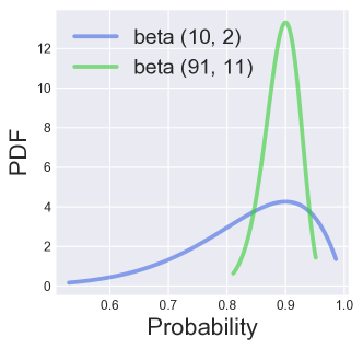
(a) Beta PDF

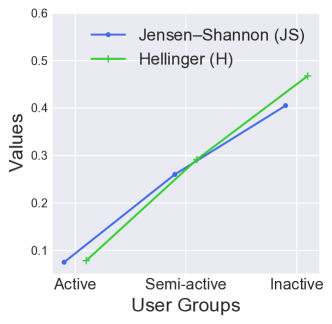
(b) Miscalibration in Test vs. Train

Figure 1. Calibration for users with different profile size

Here we present the desired properties of calibrated recommendations and explain how they affect the final recommendation before moving into our proposed model addressing them.

P1: Relevance Property. Calibrated recommendations intend to reflect different interests of users, as indicated by their interaction history, with the same proportion in the recommended list. A greedy algorithm is often proposed to re-rank a baseline recommendation list. The first desired property is that calibrating categories should occur without sacrificing overall relevance to users. Seymen et al. (2021) illustrate that greedy calibrated algorithms such as (Steck, 2018; Oh et al., 2011) fail to meet this essential requirement, leading to suboptimal recommendations.

P2: Diversity Aspects. Diversity is defined in literature as minimal redundancy or similarity among the recommended items. Various research has been proposed to generate diverse recommendations (Bhaskara et al., 2016; Zhang and Hurley, 2008; Hurley and Zhang, 2011) . An alternative research direction focuses on achieving personalized diversity, i.e., recommendations should reflect the diverse interests of users with the correct proportion (Dang and Croft, 2012; Vargas et al., 2014; Eskandanian et al., 2017; Sonboli et al., 2020). A traditional calibrated recommendation follows the second approach and does not consider diversity as a separate objective that might lead to a so-called ”filter bubble” (Pariser, 2011). Imagine a user rated 70% Comedy and 30% romance movies in a world with three genres. Such users would receive the target distribution of 70%:30%:0% of the same genres in the calibrated recommended list, depriving them of the opportunity to interact with the third genre. The second desired property in calibrated recommendation is to prevent such phenomenon by preventing a reduction in overall catalog coverage and diversity in comparison to baselines.

P3: Calibration Confidence. Calibrated recommendations are solely based on users’ historical interactions. As discussed earlier, user profile sizes influence the confidence level of the calibration algorithm. Moreover, this can be viewed from a temporal perspective, where users’ tastes change over time. The more users spend time in a system interacting with items, the more we know about their future interests and vice versa. To investigate this issue, along with the theoretical analysis of the Beta distributions (see Section 1), we perform a temporal split of the data into train/test scenarios. For this example, we consider the test data as an oracle recommendation algorithm that can make perfect predictions, i.e., return the ground truth. Figure 1b shows the degree of miscalibration for the oracle algorithm as defined in Section 2.1. To analyze the miscalibration effect from the user’s perspective, we categorize users into three groups based on their activity level, i.e., number of interactions. The top 20$\%$ of users are categorized as active group while the bottom 20$\%$ are assigned inactive group, and the remainder is categorized as semi-active group. As we can see from the values of JS and H in Figure 1b, the accuracy-optimal oracle algorithm fails to calibrate the recommendation list according to genre distribution, especially for the inactive group followed by the semi-active group. This result indicates modeling the genre preference of less active users is more challenging. Considerable training data is needed to capture users’ tastes in categories with high confidence. This is also evident in Figure 1a, where we see a  0.67 higher confidence when modeling users with larger profile sizes. Hence, calibrating recommendations for all users to the same degree regardless of their profile size leads to undesired recommendations. This raises the need for calibrated recommendations that perform better for less active users. Hence, the third desired property for calibration algorithms is varying degrees of calibration for less active users to benefit from the baseline algorithm’s predictive ability.

2.3. Proposed Model

In the following, we describe our proposed confidence-aware calibration algorithm that meets the desired properties mentioned in Section 2.2. The purpose of the algorithm is to re-rank a baseline recommendation ranking list, $L_{N}(u)$, in a way that the new top-K list, $L_{K}^{c}(u)$ where $K<N$, would reduce miscalibration without affecting the recommendation lists’ quality. To this end, we define binary matrix $Z=[Z_{ui}]_{n\times N}$ to denote whether item $i\in\mathcal{I}$ is recommended to user $u\in\mathcal{U}$ in $L_{K}^{c}(u)$. Hence, we can represent $L_{K}^{c}(u)$ as $[Z_{u1},Z_{u2},...,Z_{uN}]$ when $\sum_{i=1}^{N}{Z_{ui}}=K$. Let $W(I_{u})\in[0,1]$ denote the confidence weight given to user $u$ based on the rated items in her profile, $I_{u}$. The confidence weight aims to represent the degree of calibration for user $u$ where $1$ indicate that the model would fully calibrate the user’s historical preference in the recommended list while $0$ indicates no calibration. We can formalize the calibration optimization problem given the binary decision matrix, $Z$, as:

(3) $$\max_{Z_{ui}} \sum_{u\in\mathcal{U}}\sum_{i=1}^{N}{S_{ui}\cdot Z_{ui}}-\lambda_{1}\cdot\mathbf{MC}(Z^{1},\mathcal{U})$$

s.t. $$\sum_{i=1}^{N}{Z_{ui}}=K\quad,\sum_{i=1}^{N}{Z^{1}_{ui}}=int(W(I_{u})\cdot K) \forall u$$

$$Z^{1}_{ui}+Z^{2}_{ui}=Z_{ui}\quad,Z^{1}_{ui}~{},Z^{2}_{ui}~{},Z_{ui}\in{\{0,1\}} \forall u,i$$

where $Z^{1}_{ui}$ and $Z^{2}_{ui}$ are helper binary decision variables that indicate whether the item $Z_{ui}$ is selected due to improving miscalibration metric or a high predictive relevance score, respectively. The $int(.)$ function rounds the input to the nearest integer value. In our experiment, we define $W(I_{u})$ based on the users’ profile size, formally as $W(I_{u})=\min[\frac{|I_{u}|}{\frac{1}{\mathcal{|U|}}\sum_{u\in\mathcal{U}}|I_{u}|},1]$ motivated by our analysis in Figure 1b and leave more rigorous definitions for future work. Additionally, as described in Section 2.1, $\mathbf{MC}$ represents the miscalibration metric by calculating the average divergence values for all users on a subset of the top-K list by size $int(W(I_{u})\cdot K)$ denoted by $Z^{1}$ decision matrix. Given that the JS and H divergence functions are non-linear, for optimization purposes we adopt the Total Variation function (Chambolle, 2004; Levin and Peres, 2017) defined as the $\mathscr{l}_{1}$ norm between distributions of $p(c|u)$ and $q(c|u)$ to calculate divergence values. As a result of the linear objective function, the optimization problem becomes mixed-integer linear programming (MILP) that can be solved using heuristic algorithms (e.g., branch&bound algorithms) in industrial optimization solvers to provide a satisfactory solution in practice. Note that our proposed model will obviously satisfy properties P1 and P2 when $\lambda_{1}=0$ as it will return the same baseline recommendation and will calibrate the recommendation list completely for all users when $W(I_{u})=1~{}\forall u$ and $\lambda_{1}$ is large. Varying weighting parameter $W(I_{u})$ aims to satisfy the property P3.

3. Experiments and Results

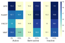
Figure 2. User groups’ catalog coverage on different models.

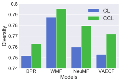
(a) MovieLens1M

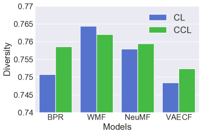
(b) MovieLensSmall

Figure 3. Diversity metric in CL and CCL model for baselines.

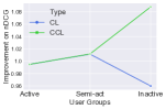
(a) nDCG

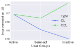
(b) Miscalibration

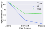
(c) Diversity

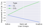
(d) Catalog Coverage

Figure 4. Improvement from the user’s perspective over baselines on various performance aspects on MovieLens1M

Table 1. The recommendation performance of our re-ranking method and corresponding baselines on MovieLensSmall and MovieLens1M datasets. The evaluation metrics here are calculated based on the top-20 predictions in the test set. Our best results are highlighted in bold. $\dagger$ and $\ddagger$ signs show the t-test p-value significance at 0.05 compared to N and CL, respectively.

Model Type MovieLensSmall MovieLens1M Precision Recall nDCG CatCov $\uparrow$ JS $\downarrow$ H $\downarrow$ Precision Recall nDCG CatCov $\uparrow$ JS $\downarrow$ H $\downarrow$ BPR N 0.0605 0.0668 0.0650 14.133 0.290 0.318 0.0769 0.0645 0.0813 11.221 0.338 0.377 CL 0.0607 0.0673 0.0668 14.193 0.130 0.144 0.0787 0.0664 0.0841 10.306 0.213 0.246 CCL 0.0630^†‡ 0.0712^†‡ 0.0693^†‡ 17.303^†‡ 0.221 0.244 0.0797^† 0.0689^†‡ 0.0853^† 12.637^†‡ 0.228 0.261 WMF N 0.0622 0.0806 0.0667 14.929 0.275 0.302 0.0629 0.0583 0.0682 11.238 0.376 0.420 CL 0.0626 0.0820 0.0651 14.331 0.125 0.140 0.0648 0.0597 0.0682 10.455 0.230 0.264 CCL 0.0652^†‡ 0.0847^†‡ 0.0693^†‡ 16.159^†‡ 0.210 0.232 0.0649^† 0.0601^† 0.0684 12.604^†‡ 0.243 0.278 NeuMF N 0.0659 0.0784 0.0721 14.911 0.282 0.311 0.1006 0.0979 0.1071 11.797 0.337 0.375 CL 0.0675 0.0766 0.0731 14.399 0.128 0.142 0.0999 0.0987 0.1057 10.940 0.199 0.227 CCL 0.0682^† 0.0809^†‡ 0.0729 17.469^†‡ 0.209 0.231 0.1010 0.1013^†‡ 0.1074 13.485^†‡ 0.225 0.258 VAECF N 0.0587 0.0672 0.0655 13.883 0.294 0.322 0.0960 0.0935 0.1019 11.543 0.334 0.372 CL 0.0627 0.0741 0.0703 14.323 0.136 0.150 0.0962 0.0946 0.1028 10.814 0.202 0.231 CCL 0.0634^† 0.0743^† 0.0713^† 16.903^†‡ 0.208 0.228 0.0966 0.0964^†‡ 0.1032 13.272^†‡ 0.226 0.259

To this end, we compare our confidence-aware calibration algorithm (CCL) against baselines (N) and a variation of our model, (CL), where $W(I_{u})=1,\forall u\in\mathcal{U}$ and hence the recommendation list is fully calibrated for all users. CL closely resembles to optimally tuned version of the prior work by Seymen et al. (2021) for all users as a comparison with the state-of-the-art calibrated model.

Experimental Settings. We use MovieLensSmall and MovieLens1M for our experiments. The MovieLensSmall contains $8974$ movies, $670$ users and $18$ item types (genres) and MovieLens1M includes $3260$ movies, $6040$ users and $18$ genres. Both datasets include explicit ratings between $1$ and $5$. We performed a temporal split on rating data into train and test sets in ratios of $80$% and $20$%, respectively. We estimate the rating matrix with BPR (Rendle et al., 2012), WMF (Hu et al., 2008), NeuMF (He et al., 2017), and VAECF (Liang et al., 2018) implemented in Cornac which is a Python-based recommender system framework (Salah et al., 2020; Truong et al., 2021) with their default hyperparameter in original paper. All baseline algorithms share the same train and test datasets. We treated the model parameter $\lambda_{1}$ as a hyperparameter and set them to the value that maximizes the $nDCG/\mathbf{MC}$. We then compare the algorithms on Precision, Recall, nDCG, JS $\&$ H divergence (see Section 2.1), Diversity (Shani and Gunawardana, 2011), and Catalog Coverage (Vargas et al., 2014) as evaluation metrics.

Relevance Aspect. We report the recommendation performance in terms of Precision, Recall, and nDCG. As seen in Table 1, our proposed model achieves higher accuracy metrics than baseline models and CL, satisfying property P1. In the MovieLensSmall dataset, the average improvements in (Precision, Recall, nDCG) were (5%, 6.1%, 5%) and (2.5%, 3.70%, 2.7%) over N and CL, respectively. We observe a similar pattern in the Movielens1M dataset. In general, we observe that neural-based baseline models achieve higher accuracy metrics, with NeuMF having the best performance..

Diversity Aspect. Figure 3 represents the diversity of CCL and CL models on both datasets. When comparing the CCL and CL models, we realize that the CCL model increases the diversity of recommendations satisfying property P2. The magnitude of this increase differs between the two datasets, with a higher increase in MovieLens1M. Concerning baselines, we find the highest level of diversity in the WMF model, followed by NeuMF, indicating the inherent ability of such algorithms to incorporate relevant, diverse items in their top ranking list.

Figure 2 depicts the catalog coverage of the CL and CCL models from the user’s perspective. CCL model achieves significantly higher catalog coverage for inactive and semi-active groups. Furthermore, active user group catalog coverage remains relatively constant compared to CL. In avoiding potential filter bubbles, this result is desirable and achieves property P2. The reason is that the profile history of active users can often predict their taste toward categories (see Figure 1b), so these users benefit from recommendations from the categories they like to interact with. In contrast, the catalog coverage of the recommendation list for inactive users (newer users) is considerably expanded to expose them to various genres and alleviate filter bubbles. Users who are semi-active fall between the two extremes.

Calibration Confidence. Figure 4 illustrates CL and CCL performance improvement compared to baselines from the user’s perspective in terms of diversity, catalog coverage, nDCG, and miscalibration measured by JS divergence. For active users, in all aspects, CL and CCL models achieve similar and significant improvements compared to N. However, for inactive users, CCL leads to a higher degree of miscalibration, despite improving on all other measures. In other words, a higher degree of miscalibration in CCL (compared to CL) benefits inactive users by providing them with more relevant and diverse (measured by diversity and catalog coverage) recommendations. This emphasizes the challenge of recommendations for cold-start users. The performance of semi-active users falls in between these two categories. Hence, considering users’ dynamic taste over time and not limiting baseline models’ predictive abilities (i.e., following property P3) can benefit less active users, which our proposed CCL model captures.

4. Conclusions and Future Work

In this paper, we highlighted the desired properties in various aspects of calibration and motivated their importance. We then proposed a multi-objective mixed integer linear programming method to recommend a calibrated top-K recommendation. Extensive experiments on two datasets and four state-of-the-art recommendation algorithms confirm that our method can calibrate the recommendation list and simultaneously increase diversity and accuracy while accounting for calibration confidence. In the future, we plan to study calibration on various beyond-accuracy aspects, such as calibrating over degrees of interest towards popular items.

- (1)
- Abdollahpouri et al. (2020) Himan Abdollahpouri, Masoud Mansoury, Robin Burke, and Bamshad Mobasher. 2020. The connection between popularity bias, calibration, and fairness in recommendation. In Fourteenth ACM conference on recommender systems. 726–731.
- Bella et al. (2010) Antonio Bella, Cèsar Ferri, José Hernández-Orallo, and María José Ramírez-Quintana. 2010. Calibration of machine learning models. In Handbook of Research on Machine Learning Applications and Trends: Algorithms, Methods, and Techniques. IGI Global, 128–146.
- Bhaskara et al. (2016) Aditya Bhaskara, Mehrdad Ghadiri, Vahab Mirrokni, and Ola Svensson. 2016. Linear relaxations for finding diverse elements in metric spaces. Advances in neural information processing systems 29 (2016).
- Chambolle (2004) Antonin Chambolle. 2004. An algorithm for total variation minimization and applications. Journal of Mathematical imaging and vision 20, 1 (2004), 89–97.
- Dang and Croft (2012) Van Dang and W Bruce Croft. 2012. Diversity by proportionality: an election-based approach to search result diversification. In Proceedings of the 35th international ACM SIGIR conference on Research and development in information retrieval. 65–74.
- Eskandanian et al. (2017) Farzad Eskandanian, Bamshad Mobasher, and Robin Burke. 2017. A Clustering Approach for Personalizing Diversity in Collaborative Recommender Systems. In Proceedings of the 25th Conference on User Modeling, Adaptation and Personalization (Bratislava, Slovakia) (UMAP ’17). Association for Computing Machinery, New York, NY, USA, 280–284. https://doi.org/10.1145/3079628.3079699
- He et al. (2017) Xiangnan He, Lizi Liao, Hanwang Zhang, Liqiang Nie, Xia Hu, and Tat-Seng Chua. 2017. Neural collaborative filtering. In Proceedings of the 26th international conference on world wide web. 173–182.
- Hu et al. (2008) Yifan Hu, Yehuda Koren, and Chris Volinsky. 2008. Collaborative filtering for implicit feedback datasets. In 2008 Eighth IEEE international conference on data mining. Ieee, 263–272.
- Hurley and Zhang (2011) Neil Hurley and Mi Zhang. 2011. Novelty and diversity in top-n recommendation–analysis and evaluation. ACM Transactions on Internet Technology (TOIT) 10, 4 (2011), 1–30.
- Levin and Peres (2017) David A Levin and Yuval Peres. 2017. Markov chains and mixing times. Vol. 107. American Mathematical Soc.
- Liang et al. (2018) Dawen Liang, Rahul G Krishnan, Matthew D Hoffman, and Tony Jebara. 2018. Variational autoencoders for collaborative filtering. In Proceedings of the 2018 world wide web conference. 689–698.
- Lin et al. (2020) Kun Lin, Nasim Sonboli, Bamshad Mobasher, and Robin Burke. 2020. Calibration in Collaborative Filtering Recommender Systems: A User-Centered Analysis. In Proceedings of the 31st ACM Conference on Hypertext and Social Media (Virtual Event, USA) (HT ’20). Association for Computing Machinery, New York, NY, USA, 197–206. https://doi.org/10.1145/3372923.3404793
- Oh et al. (2011) Jinoh Oh, Sun Park, Hwanjo Yu, Min Song, and Seung-Taek Park. 2011. Novel recommendation based on personal popularity tendency. In 2011 IEEE 11th International Conference on Data Mining. IEEE, 507–516.
- Pariser (2011) Eli Pariser. 2011. The filter bubble: What the Internet is hiding from you. Penguin UK.
- Rendle et al. (2012) Steffen Rendle, Christoph Freudenthaler, Zeno Gantner, and Lars Schmidt-Thieme. 2012. BPR: Bayesian personalized ranking from implicit feedback. arXiv preprint arXiv:1205.2618 (2012).
- Salah et al. (2020) Aghiles Salah, Quoc-Tuan Truong, and Hady W Lauw. 2020. Cornac: A Comparative Framework for Multimodal Recommender Systems. Journal of Machine Learning Research 21, 95 (2020), 1–5.
- Seymen et al. (2021) Sinan Seymen, Himan Abdollahpouri, and Edward C Malthouse. 2021. A Constrained Optimization Approach for Calibrated Recommendations. In Fifteenth ACM Conference on Recommender Systems. 607–612.
- Shani and Gunawardana (2011) Guy Shani and Asela Gunawardana. 2011. Evaluating recommendation systems. In Recommender systems handbook. Springer, 257–297.
- Sonboli et al. (2020) Nasim Sonboli, Farzad Eskandanian, Robin Burke, Weiwen Liu, and Bamshad Mobasher. 2020. Opportunistic Multi-Aspect Fairness through Personalized Re-Ranking. In Proceedings of the 28th ACM Conference on User Modeling, Adaptation and Personalization (Genoa, Italy) (UMAP ’20). Association for Computing Machinery, New York, NY, USA, 239–247. https://doi.org/10.1145/3340631.3394846
- Steck (2018) Harald Steck. 2018. Calibrated recommendations. In Proceedings of the 12th ACM conference on recommender systems. 154–162.
- Truong et al. (2021) Quoc-Tuan Truong, Aghiles Salah, Thanh-Binh Tran, Jingyao Guo, and Hady W Lauw. 2021. Exploring Cross-Modality Utilization in Recommender Systems. IEEE Internet Computing (2021).
- Vargas et al. (2014) Saúl Vargas, Linas Baltrunas, Alexandros Karatzoglou, and Pablo Castells. 2014. Coverage, redundancy and size-awareness in genre diversity for recommender systems. In Proceedings of the 8th ACM Conference on Recommender systems. 209–216.
- Wang et al. (2013) Yining Wang, Liwei Wang, Yuanzhi Li, Di He, and Tie-Yan Liu. 2013. A theoretical analysis of NDCG type ranking measures. In Conference on learning theory. PMLR, 25–54.
- Zhang and Hurley (2008) Mi Zhang and Neil Hurley. 2008. Avoiding monotony: improving the diversity of recommendation lists. In Proceedings of the 2008 ACM conference on Recommender systems. 123–130.