NOSMOG: Learning Noise-robust and Structure-aware MLPs on Graphs

Abstract

While Graph Neural Networks (GNNs) have demonstrated their efficacy in dealing with non-Euclidean structural data, they are difficult to be deployed in real applications due to the scalability constraint imposed by multi-hop data dependency. Existing methods attempt to address this scalability issue by training multi-layer perceptrons (MLPs) exclusively on node content features using labels derived from trained GNNs. Even though the performance of MLPs can be significantly improved, two issues prevent MLPs from outperforming GNNs and being used in practice: the ignorance of graph structural information and the sensitivity to node feature noises. In this paper, we propose to learn NOise-robust Structure-aware MLPs On Graphs (NOSMOG) to overcome the challenges. Specifically, we first complement node content with position features to help MLPs capture graph structural information. We then design a novel representational similarity distillation strategy to inject structural node similarities into MLPs. Finally, we introduce the adversarial feature augmentation to ensure stable learning against feature noises and further improve performance. Extensive experiments demonstrate that NOSMOG outperforms GNNs and the state-of-the-art method in both transductive and inductive settings across seven datasets, while maintaining a competitive inference efficiency. Codes are available at https://github.com/meettyj/NOSMOG.

1 Introduction

Graph Neural Networks (GNNs) have shown exceptional effectiveness in handling non-Euclidean structural data and have achieved state-of-the-art performance across a broad range of graph mining tasks [9, 15, 31]. The success of modern GNNs relies on the usage of message passing architecture, which aggregates and learns node representations based on their (multi-hop) neighborhood [34, 46]. However, message passing is time-consuming and computation-intensive, making it challenging to apply GNNs to real large-scale applications that are always constrained by latency and require the deployed model to infer fast [43, 41, 13]. To meet the latency requirement, multi-layer perceptrons (MLPs) continue to be the first choice [44], despite the fact that they perform poorly in non-euclidean graph data and focus exclusively on the node content information.

Inspired by the performance advantage of GNNs and the latency advantage of MLPs, researchers start wondering if they could combine GNNs and MLPs together to enjoy the advantages of both [12, 44, 45, 2]. To combine them, one effective approach is to use knowledge distillation (KD) [10, 7], where the learned knowledge is transferred from GNNs to MLPs through soft labels [25]. Then only MLPs are deployed for inference, with node content features as input. In this way, MLPs can perform well by mimicking the output of GNNs without requiring explicit message passing, and thus obtaining a fast inference speed [12]. Nevertheless, existing methods have two major drawbacks: (1) MLPs cannot fully capture the graph structural information or explicitly learn node relations with only node content features as input; and (2) MLPs are sensitive to node feature noises that can easily destroy the performance. We thus ask: Can we learn MLPs that are graph structure-aware and insensitive to node feature noises, meanwhile performing better than GNNs and inferring fast?

To address these issues and answer the question, we propose to learn NOise-robust Structure-aware MLPs On Graphs (NOSMOG) with remarkable performance and inference speed. Specifically, we first extract node position features from the graph and combine them with node content features as the input of MLPs. Thus MLPs can fully capture the graph structure as well as the node positional information. Then, we design a novel representational similarity distillation strategy to transfer the node similarity information from GNNs to MLPs, so that MLPs can encode the structural node affinity and learn more effectively from GNNs through hidden layer representations. After that, we introduce the adversarial feature augmentation to make MLPs noise-resistant and further improve the performance. To fully evaluate our model, we conduct extensive experiments on 7 public benchmark datasets in both transductive and inductive settings. We conclude that NOSMOG can capture graph structure and become robust to noises by incorporating position features, representational similarity, and training with adversarial learning. At the same time, NOSMOG can improve the state-of-the-art method and even outperform GNNs, while maintaining a fast inference speed. Particularly, NOSMOG improves GNNs by 2.05%, MLPs by 25.22%, and existing state-of-the-art method by 6.63%, averaged across 7 datasets and 2 settings. In the meantime, NOSMOG achieves comparable efficiency to the state-of-the-art method and is 833× faster than GNNs with the same number of layers. To summarize, the contributions of this paper are as follows:

• We point out that existing GNNs-MLPs KD frameworks suffer from two major issues that undermine their applicability and reliability: the ignorance of graph structural information and the sensitivity to node feature noises.

• To address the challenges, we propose to learn Noise-robust and Structure-aware MLPs on Graphs. The proposed model contains three key components: the incorporation of position features, representational similarity distillation, and adversarial feature augmentation.

• Extensive experiments demonstrate that NOSMOG can easily outperform GNNs and the state-of-the-art method. In addition, we present robustness analysis, efficiency comparison, ablation studies, and theoretical explanation to better understand the effectiveness of the proposed model.

2 Related Work

Graph Neural Networks. Many graph neural networks [15, 31, 9, 19, 3] were proposed to encode the graph-structure data. They take advantage of the message passing paradigm by aggregating neighborhood information to learn node embeddings. For example, GCN [15] introduces a layer-wise propagation rule to learn node features. GAT [31] incorporates an attention mechanism to aggregate features from neighbors with different weights. GraphSAGE [9] applies an efficient aggregation function to learn node features from the local neighborhood. DeepGCNs [19] and GCNII [3] utilize residual connections to aggregate neighbors from multi-hop and further address the over-smoothing problem. However, These message passing GNNs only leverage local graph structure and have been demonstrated to be no more powerful than the WL graph isomorphism test [36, 23]. Recent works propose to empower graph learning with positional encoding techniques such as Laplacian Eigenmap and DeepWalk [40, 33, 20, 24, 27], so that the node’s position within the broader context of the graph structure can be detected. Inspired by these studies, we incorporate position features to fully capture the graph structure and node positional information.

Knowledge Distillation on Graph. Knowledge Distillation (KD) has been applied widely in graph-based research and GNNs [18, 39, 37, 38, 28, 8]. Previous works apply KD primarily to learn student GNNs with fewer parameters but perform as well as the teacher GNNs. However, time-consuming message passing with multi-hop neighborhood fetching is still required during the learning process. For example, LSP [39] and TinyGNN [37] fetch and aggregate neighbor information by introducing the local structure-preserving and peer-aware modules that rely heavily on message passing. To overcome the latency issues, recent works start focusing on learning an MLP-based student model that does not require message passing [12, 44, 45]. Specifically, MLP student is trained with node content features as input and soft labels from GNN teacher as targets. Although MLP can mimic GNN’s prediction, the graph structural information is explicitly overlooked from the input, resulting in incomplete learning, and the student is highly susceptible to noises that may be present in the feature. In our work, we address these concerns. Correspondingly, since adversarial learning has shown great performance in handling feature noises and enhancing modle learning capability [14, 35, 17, 29, 48], we introduce the adversarial feature augmentation to ensure stable learning against noises and further improve performance.

3 Preliminary

Notations. A graph is usually denoted as ${\mathcal{G}}=(\mathcal{V},\mathcal{E},{\bm{C}})$, where $\mathcal{V}$ represents the node set, $\mathcal{E}$ represents the edge set, ${\bm{C}}\in\mathbb{R}^{N\times d_{c}}$ stands for the $d_{c}$-dimensional node content attributes, and $N$ is the total number of nodes. In the node classification task, the model tries to predict the category probability for each node $v\in\mathcal{V}$, supervised by the ground truth node category ${\bm{Y}}\in\mathbb{R}^{K}$, where $K$ is the number of categories. We use superscript ^L to mark the properties of labeled nodes (i.e., $\mathcal{V}^{L}$, ${\bm{C}}^{L}$, and ${\bm{Y}}^{L}$), and superscript ^U to mark the properties of unlabeled nodes (i.e., $\mathcal{V}^{U}$, ${\bm{C}}^{U}$, and ${\bm{Y}}^{U}$).

Graph Neural Networks. For a given node $v\in\mathcal{V}$, GNNs aggregate the messages from node neighbors $\mathcal{N}(v)$ to learn node embedding ${\bm{h}}_{v}\in\mathbb{R}^{d_{n}}$ with dimension $d_{n}$. Specifically, the node embedding in $l$-th layer ${\bm{h}}_{v}^{(l)}$ is learned by first aggregating (AGG) the neighbor embeddings and then combining (COM) it with the embedding from the previous layer. The whole learning process can be denoted as: ${\bm{h}}_{v}^{(l)}=\textsc{COM}({\bm{h}}_{v}^{(l-1)},\textsc{AGG}(\{{\bm{h}}_{u}^{(l-1)}:u\in\mathcal{N}(v)\}))$.

4 Proposed Model

In this section, we present the details of NOSMOG. An overview of the proposed model is shown in Figure 1. We introduce NOSMOG by first introducing the background of training MLPs with GNNs distillation, and then illustrating three key components in NOSMOG, i.e., the incorporation of position features (Figure 1 (b)), representational similarity distillation (Figure 1 (c)), and adversarial feature augmentation (Figure 1 (d)).

Training MLPs with GNNs Distillation. The key idea of training MLPs with the knowledge distilled from GNNs is simple. Given a cumbersome pre-trained GNN, the ground truth label ${\bm{y}}_{v}$ for any labeled node $v\in\mathcal{V}^{L}$, and the soft label ${\bm{z}}_{v}$ learned by the teacher GNN for any node $v\in\mathcal{V}$, the goal is to train a lightweight MLP using both ground truth labels and soft labels. The objective function can be formulated as:

$$\mathcal{L}=\sum_{v\in\mathcal{V}^{L}}\mathcal{L}_{GT}(\hat{\bm{y}}_{v},{\bm{y}}_{v})+\lambda\sum_{v\in\mathcal{V}}\mathcal{L}_{SL}(\hat{\bm{y}}_{v},{\bm{z}}_{v}),$$ (1)

where $\mathcal{L}_{GT}$ is the cross-entropy loss between the student prediction $\hat{\bm{y}}_{v}$ and the ground truth label ${\bm{y}}_{v}$, $\mathcal{L}_{SL}$ is the KL-divergence loss between the student prediction $\hat{\bm{y}}_{v}$ and the soft labels ${\bm{z}}_{v}$, and $\lambda$ is a trade-off weight for balancing two losses.

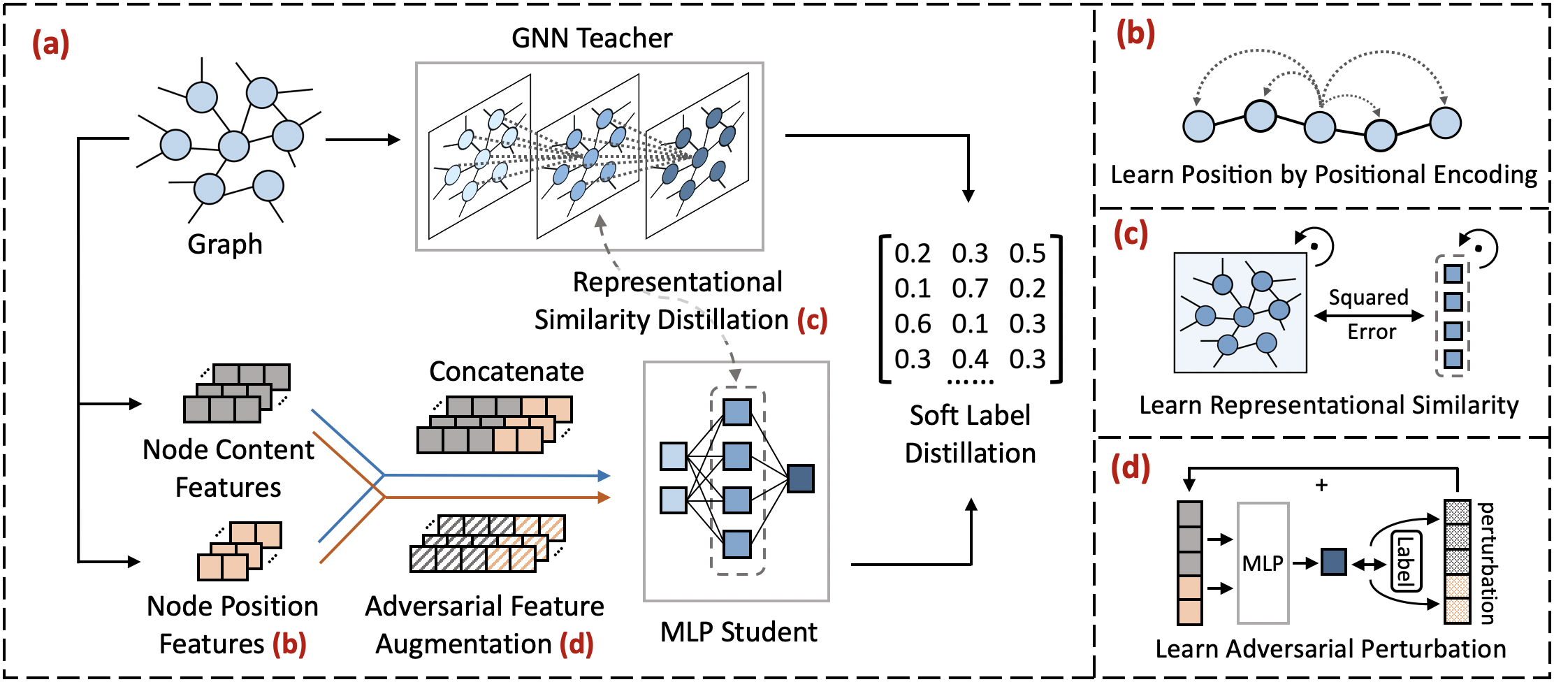
Figure 1: (a) The overall framework of NOSMOG: A GNN teacher is trained on the graph to obtain the representational node similarity and soft labels. Then, an MLP student is trained on node content features and position features, guided by the learned representational node similarity and soft labels. We also introduce the adversarial feature augmentation to ensure stable learning against feature noises and improve performance. (b) The acquisition of node position features: capturing node positional information by positional encoding techniques. (c) Representational Similarity Distillation: enforcing MLP to learn node similarity from GNN’s representation space. (d) Adversarial Feature Augmentation: learning adversarial features by generating adversarial perturbation for input features.

Incorporating Node Position Features. To empower graph learning and assist MLP in capturing node positions on graph, we propose to enrich node content by positional encoding techniques such as DeepWalk [24]. By simply concatenating the node content features with the learned position features, MLP is able to capture node positional information within a broader context of the graph structure. The idea of incorporating position features is straightforward, yet as we will see, extremely effective. Specifically, we first learn position feature ${\bm{P}}_{v}$ for node $v\in\mathcal{V}$ by running DeepWalk algorithm on ${\mathcal{G}}$. Noticed that there are no node content features involved in this step, so the position features are solely determined by the graph structure and the node positions in the graph. Then, we concatenate (CONCAT) the content feature ${\bm{C}}_{v}$ and position feature ${\bm{P}}_{v}$ to form the final node feature ${\bm{X}}_{v}$. After that, we send the concatenated node feature into MLP to obtain the category prediction $\hat{\bm{y}}_{v}$. The entire process is formulated as:

$${\bm{X}}_{v}=\textsc{CONCAT}({\bm{C}}_{v},{\bm{P}}_{v}),\quad\quad\hat{\bm{y}}_{v}=\textsc{MLP}({\bm{X}}_{v}).$$ (2)

Later, $\hat{\bm{y}}_{v}$ is leveraged to calculate $\mathcal{L}_{GT}$ and $\mathcal{L}_{SL}$ (Equation 1).

Representational Similarity Distillation. To improve MLP’s ability to learn from GNN and further capture the structural node similarity, we propose the Representational Similarity Distillation (RSD) to encourage MLP to learn from GNN’s representation space. RSD maintains the representation space by preserving the similarity between node embeddings, and leverages mean squared error to measure the similarity discrepancy between GNN and MLP. Compared to soft labels, the relative similarity between intermediate representations of different nodes serves as a more flexible and appropriate guidance from the teacher model [30]. Specifically, given the learned GNN representations ${\bm{H}}_{G}\in\mathbb{R}^{N\times d_{G}}$ and the MLP representations ${\bm{H}}_{M}\in\mathbb{R}^{N\times d_{M}}$, where $d_{G}$ and $d_{M}$ indicate the representation dimension of GNN and MLP respectively, we define the intra-model representational similarity $S_{GNN}$, $S_{MLP}$ for GNN and MLP as:

$$S_{GNN}={\bm{H}}_{G}\cdot{\bm{H}}_{G}\quad\quad\mathrm{and}\quad\quad S_{MLP}={\bm{H}}_{M}^{\prime}\cdot{\bm{H}}_{M}^{\prime},\quad{\bm{H}}_{M}^{\prime}=\sigma(W_{M}\cdot{\bm{H}}_{M}),$$ (3)

where $W_{M}\in\mathbb{R}^{d_{M}\times d_{M}}$ is the transformation matrix to map MLP representations into GNN representation space, $\sigma$ is the activation function (we use ReLU in this work), and ${\bm{H}}_{M}^{\prime}$ is the transformed MLP representations. We then define the RSD loss $\mathcal{L}_{RSD}$ to minimize the inter-model representation similarity:

$$\mathcal{L}_{RSD}(S_{GNN},S_{MLP})=||S_{GNN}-S_{MLP}||_{F}^{2},$$ (4)

where $||\cdot||_{F}$ is the Frobenius norm.

Adversarial Feature Augmentation. MLP is highly susceptible to feature noises [6] if only considers the explicit feature information associated with each node. To enhance MLP’s robustness to noises, we introduce the adversarial feature augmentation to leverage the regularization power of adversarial features [4, 17, 42]. In other words, adversarial feature augmentation makes MLP invariant to small fluctuations in the features and generalizes to out-of-distribution samples, with the ability to further boost performance [32, 5]. Compared to the vanilla training that we send original node content features ${\bm{C}}$ into MLP to obtain the category prediction, adversarial training learns the perturbation $\delta$ and sends maliciously perturbed features ${\bm{C}}+\delta$ as input for MLP to learn. This process can be formulated as the following min-max optimization problem:

$$\min_{\bm{\theta}}\left[\max_{\|\delta\|_{p}\leq\epsilon}\left(-{\bm{Y}}\log(\textsc{MLP}({\bm{C}}+\delta))\right)\right],$$ (5)

where $\bm{\theta}$ represents the model parameters, $\delta$ is the perturbation, $\|\cdot\|_{p}$ is the $\ell_{p}$-norm distance metric, and $\epsilon$ is the perturbation range. Specifically, we choose Projected Gradient Descent [22] as the default attacker to generate adversarial perturbation iteratively:

$$\delta_{t+1}=\Pi_{\|\delta\|_{\infty}\leq\epsilon}\left[\delta_{t}+{\bm{s}}\cdot\text{sign}\left(\nabla_{\delta}\left(-{\bm{Y}}\log(\textsc{MLP}({\bm{C}}+\delta_{t}))\right)\right)\right],$$ (6)

where ${\bm{s}}$ is the perturbation step size and $\nabla_{\delta}$ is the calculated gradient given $\delta$. For maximum robustness, the final perturbation $\delta=\delta_{T}$ is learned by updating Equation 6 for $T$ times to generate the worst-case noises. Finally, to accommodate KD, we perform adversarial training using both ground truth labels ${\bm{y}}_{v}$ for labeled nodes ($v\in\mathcal{V}^{L}$), and soft labels ${\bm{z}}_{v}$ for all nodes in graph ($v\in\mathcal{V}$). Therefore, we can reformulate the objective in Equation 5 as follows:

$${\bm{C}}_{v}^{\prime} ={\bm{C}}_{v}+\delta,\quad\quad\quad\hat{\bm{y}}_{v}^{\prime}=\textsc{MLP}({\bm{C}}_{v}^{\prime}),$$ (7)

$$\mathcal{L}_{ADV} =\max_{\delta\in\epsilon}[-\sum_{v\in\mathcal{V}^{L}}{\bm{y}}_{v}\log(\hat{\bm{y}}_{v}^{\prime})-\sum_{v\in\mathcal{V}}{\bm{z}}_{v}\log(\hat{\bm{y}}_{v}^{\prime})].$$

The final objective function $\mathcal{L}$ is defined as the weighted combination of ground truth cross-entropy loss $\mathcal{L}_{GT}$, soft label distillation loss $\mathcal{L}_{SL}$, representational similarity distillation loss $\mathcal{L}_{RSD}$ and adversarial learning loss $\mathcal{L}_{ADV}$:

$$\mathcal{L}=\mathcal{L}_{GT}+\lambda\mathcal{L}_{SL}+\mu\mathcal{L}_{RSD}+\eta\mathcal{L}_{ADV},$$ (8)

where $\lambda$, $\mu$ and $\eta$ are trade-off weights for balancing $\mathcal{L}_{SL}$, $\mathcal{L}_{RSD}$ and $\mathcal{L}_{ADV}$, respectively.

5 Experiments

In this section, we conduct extensive experiments to validate the effectiveness of the proposed model and answer the following questions: 1) Can NOSMOG outperform GNNs, MLPs, and other GNNs-MLPs methods? 2) Can NOSMOG work well under both inductive and transductive settings? 3) Can NOSMOG work well with noisy features? 4) How does NOSMOG perform in terms of inference time? 5) How does NOSMOG perform with different model components? 6) How does NOSMOG perform with different teacher GNNs? 7) How can we explain the superior performance of NOSMOG?

5.1 Experiment Settings

Datasets. We use five widely used public benchmark datasets [44, 38] (i.e., Cora, Citeseer, Pubmed, A-computer, and A-photo), and two large OGB datasets [11] (i.e., Arxiv and Products) to evaluate the proposed model.
Model Architectures. For a fair comparison, we follow the paper [44] to use GraphSAGE [9] with GCN aggregation as the teacher model. However, we also show the impact of other teacher models including GCN [15], GAT [31] and APPNP [16] in Section 5.7.
Evaluation Protocol. For experiments, we report the mean and standard deviation of ten separate runs with different random seeds. We adopt accuracy to measure the model performance, use validation data to select the optimal model, and report the results on test data.
Two Settings: Transductive vs. Inductive. To fully evaluate the model, we conduct node classification in two settings: transductive (tran) and inductive (ind). For tran, we train models on ${\mathcal{G}}$, ${\bm{X}}^{L}$, and ${\bm{Y}}^{L}$, while evaluate them on ${\bm{X}}^{U}$ and ${\bm{Y}}^{U}$. We generate soft labels for every nodes in the graph (i.e., ${\bm{z}}_{v}$ for $v\in\mathcal{V}$). For ind, we follow previous work [44] to randomly select out 20% test data for inductive evaluation. Specifically, we separate the unlabeled nodes $\mathcal{V}^{U}$ into two disjoint observed and inductive subsets (i.e., $\mathcal{V}^{U}=\mathcal{V}^{U}_{obs}\sqcup\mathcal{V}^{U}_{ind}$), which leads to three separate graphs ${\mathcal{G}}={\mathcal{G}}^{L}\sqcup{\mathcal{G}}_{obs}^{U}\sqcup{\mathcal{G}}_{ind}^{U}$ with no shared nodes. The edges between ${\mathcal{G}}^{L}\sqcup{\mathcal{G}}_{obs}^{U}$ and ${\mathcal{G}}_{ind}^{U}$ are removed during training but are used during inference to transfer position features by average operator [9]. Node features and labels are partitioned into three disjoint sets, i.e., ${\bm{X}}={\bm{X}}^{L}\sqcup{\bm{X}}_{obs}^{U}\sqcup{\bm{X}}_{ind}^{U}$ and ${\bm{Y}}={\bm{Y}}^{L}\sqcup{\bm{Y}}_{obs}^{U}\sqcup{\bm{Y}}_{ind}^{U}$. We generate soft labels for nodes in the labeled and observed subsets (i.e., ${\bm{z}}_{v}$ for $v\in\mathcal{V}^{L}\sqcup\mathcal{V}^{U}_{obs}$). Our code will be released upon publication.

5.2 Can NOSMOG outperform GNNs, MLPs, and other GNNs-MLPs methods?

We compare our model NOSMOG to GNN, MLP, and the state-of-the-art methods with the same experimental settings. We first consider the standard transductive setting, so our results in Table 1 are directly comparable to those reported in previous literatures [44, 11, 38]. As shown in Table 1, NOSMOG outperforms both teacher model and baseline methods on all datasets. Compared to the teacher GNN, NOSMOG improves the performance by 2.46% on average across different datasets, which demonstrates that NOSMOG can capture better structural information than GNN without explicit graph structure input. Compared to MLP, NOSMOG improves the performance by 26.29% on average across datasets, while the state-of-the-art method GLNN [44] can only improve MLP by 18.55%, which shows the efficacy of KD and demonstrates that NOSMOG can capture additional information that GLNN cannot. Compared to GLNN, NOSMOG improves the performance by 6.86% on average across datasets. Specifically, GLNN performs poorly in large OGB datasets (the last 2 rows) while NOSMOG learns well and shows an improvement of 12.39% and 23.14%, respectively. This further demonstrates the effectiveness of NOSMOG. The analyses of the capability of each model component and the expressiveness of NOSMOG are shown in Sections 5.6 and 5.8, respectively.

Table 1: NOSMOG outperforms GNN, MLP, and the state-of-the-art method GLNN on all datasets under the standard setting. $\Delta_{GNN}$, $\Delta_{MLP}$, $\Delta_{GLNN}$ represents the difference between the NOSMOG and GNN, MLP, GLNN, respectively. Results show accuracy (higher is better).

Datasets SAGE MLP GLNN NOSMOG $\Delta_{GNN}$ $\Delta_{MLP}$ $\Delta_{GLNN}$ Cora 80.64 $\pm$ 1.57 59.18 $\pm$ 1.60 80.26 $\pm$ 1.66 83.04 $\pm$ 1.26 $\uparrow$ 2.98% $\uparrow$ 40.32% $\uparrow$ 3.46% Citeseer 70.49 $\pm$ 1.53 58.50 $\pm$ 1.86 71.22 $\pm$ 1.50 73.78 $\pm$ 1.54 $\uparrow$ 4.67% $\uparrow$ 26.12% $\uparrow$ 3.59% Pubmed 75.56 $\pm$ 2.06 68.39 $\pm$ 3.09 75.59 $\pm$ 2.46 77.34 $\pm$ 2.36 $\uparrow$ 2.36% $\uparrow$ 13.09% $\uparrow$ 2.32% A-computer 82.82 $\pm$ 1.37 67.62 $\pm$ 2.21 82.71 $\pm$ 1.18 84.04 $\pm$ 1.01 $\uparrow$ 1.47% $\uparrow$ 24.28% $\uparrow$ 1.61% A-photo 90.85 $\pm$ 0.87 77.29 $\pm$ 1.79 91.95 $\pm$ 1.04 93.36 $\pm$ 0.69 $\uparrow$ 2.76% $\uparrow$ 20.79% $\uparrow$ 1.53% Arxiv 70.73 $\pm$ 0.35 55.67 $\pm$ 0.24 63.75 $\pm$ 0.48 71.65 $\pm$ 0.29 $\uparrow$ 1.30% $\uparrow$ 28.70% $\uparrow$ 12.39% Products 77.17 $\pm$ 0.32 60.02 $\pm$ 0.10 63.71 $\pm$ 0.31 78.45 $\pm$ 0.38 $\uparrow$ 1.66% $\uparrow$ 30.71% $\uparrow$ 23.14%

5.3 Can NOSMOG work well under both inductive and transductive settings?

To better understand the effectiveness of NOSMOG, we conduct experiments in a realistic production ($prod$) scenario that involves both inductive ($ind$) and transductive ($tran$) settings (see Table 2). We find that NOSMOG can achieve superior or comparable performance to the teacher model and baseline methods across all datasets and settings. Specifically, compared to GNN, NOSMOG achieves better performance in all datasets and settings, except for $ind$ on Arxiv and Products where NOSMOG can only achieve comparable performance. Considering these two datasets have a significant distribution shift between training data and test data [44], this is understandable that NOSMOG cannot outperform GNN without explicit graph structure input. However, compared to GLNN which can barely learn on these two datasets, NOSMOG improves the performance extensively, i.e., 18.72% and 11.01% on these two datasets, respectively. This demonstrates the capability of NOSMOG in capturing graph structural information on large-scale datasets, despite the significant distribution shift. In addition, NOSMOG outperforms MLP and GLNN by great margins in all datasets and settings, with an average of 24.15% and 6.39% improvement, respectively. Therefore, we conclude that NOSMOG can achieve exceptional performance in the production environment with both inductive and transductive settings.

Table 2: NOSMOG outperforms GNN, MLP, and the state-of-the-art method GLNN in a production scenario with both inductive and transductive settings. ind indicates the results on $\mathcal{V}^{U}_{ind}$, tran indicates the results on $\mathcal{V}^{U}_{tran}$, and prod indicates the interpolated production results of both $ind$ and $tran$.

Datasets Eval SAGE MLP GLNN NOSMOG $\Delta_{GNN}$ $\Delta_{MLP}$ $\Delta_{GLNN}$ Cora prod 79.53 59.18 77.82 81.02 $\uparrow$ 1.87% $\uparrow$ 36.90% $\uparrow$ 4.11% ind 81.03 $\pm$ 1.71 59.44 $\pm$ 3.36 73.21 $\pm$ 1.50 81.36 $\pm$ 1.53 $\uparrow$ 0.41% $\uparrow$ 36.88% $\uparrow$ 11.13% tran 79.16 $\pm$ 1.60 59.12 $\pm$ 1.49 78.97 $\pm$ 1.56 80.93 $\pm$ 1.65 $\uparrow$ 2.24% $\uparrow$ 36.89% $\uparrow$ 2.48% Citeseer prod 68.06 58.49 69.08 70.60 $\uparrow$ 3.73% $\uparrow$ 20.70% $\uparrow$ 2.20% ind 69.14 $\pm$ 2.99 59.31 $\pm$ 4.56 68.48 $\pm$ 2.38 70.30 $\pm$ 2.30 $\uparrow$ 1.68% $\uparrow$ 18.53% $\uparrow$ 2.66% tran 67.79 $\pm$ 2.80 58.29 $\pm$ 1.94 69.23 $\pm$ 2.39 70.67 $\pm$ 2.25 $\uparrow$ 4.25% $\uparrow$ 21.24% $\uparrow$ 2.08% Pubmed prod 74.77 68.39 74.67 75.82 $\uparrow$ 1.40% $\uparrow$ 10.86% $\uparrow$ 1.54% ind 75.07 $\pm$ 2.89 68.28 $\pm$ 3.25 74.52 $\pm$ 2.95 75.87 $\pm$ 3.32 $\uparrow$ 1.07% $\uparrow$ 11.12% $\uparrow$ 1.81% tran 74.70 $\pm$ 2.33 68.42 $\pm$ 3.06 74.70 $\pm$ 2.75 75.80 $\pm$ 3.06 $\uparrow$ 1.47% $\uparrow$ 10.79% $\uparrow$ 1.47% A-computer prod 82.73 67.62 82.10 83.85 $\uparrow$ 1.35% $\uparrow$ 24.00% $\uparrow$ 2.13% ind 82.83 $\pm$ 1.51 67.69 $\pm$ 2.20 80.27 $\pm$ 2.11 84.36 $\pm$ 1.57 $\uparrow$ 1.85% $\uparrow$ 24.63% $\uparrow$ 5.10% tran 82.70 $\pm$ 1.34 67.60 $\pm$ 2.23 82.56 $\pm$ 1.80 83.72 $\pm$ 1.44 $\uparrow$ 1.23% $\uparrow$ 23.85% $\uparrow$ 1.41% A-photo prod 90.45 77.29 91.34 92.47 $\uparrow$ 2.23% $\uparrow$ 19.64% $\uparrow$ 1.24% ind 90.56 $\pm$ 1.47 77.44 $\pm$ 1.50 89.50 $\pm$ 1.12 92.61 $\pm$ 1.09 $\uparrow$ 2.26% $\uparrow$ 19.59% $\uparrow$ 3.48% tran 90.42 $\pm$ 0.68 77.25 $\pm$ 1.90 91.80 $\pm$ 0.49 92.44 $\pm$ 0.51 $\uparrow$ 2.23% $\uparrow$ 19.66% $\uparrow$ 0.70% Arxiv prod 70.69 55.35 63.50 70.90 $\uparrow$ 0.30% $\uparrow$ 28.09% $\uparrow$ 11.65% ind 70.69 $\pm$ 0.58 55.29 $\pm$ 0.63 59.04 $\pm$ 0.46 70.09 $\pm$ 0.55 $\downarrow$ -0.85% $\uparrow$ 26.77% $\uparrow$ 18.72% tran 70.69 $\pm$ 0.39 55.36 $\pm$ 0.34 64.61 $\pm$ 0.15 71.10 $\pm$ 0.34 $\uparrow$ 0.58% $\uparrow$ 28.43% $\uparrow$ 10.05% Products prod 76.93 60.02 63.47 77.33 $\uparrow$ 0.52% $\uparrow$ 28.84% $\uparrow$ 21.84% ind 77.23 $\pm$ 0.24 60.02 $\pm$ 0.09 63.38 $\pm$ 0.33 77.02 $\pm$ 0.19 $\downarrow$ -0.27% $\uparrow$ 28.32% $\uparrow$ 11.01% tran 76.86 $\pm$ 0.27 60.02 $\pm$ 0.11 63.49 $\pm$ 0.31 77.41 $\pm$ 0.21 $\uparrow$ 0.72% $\uparrow$ 28.97% $\uparrow$ 21.93%

5.4 Can NOSMOG work well with noisy features?

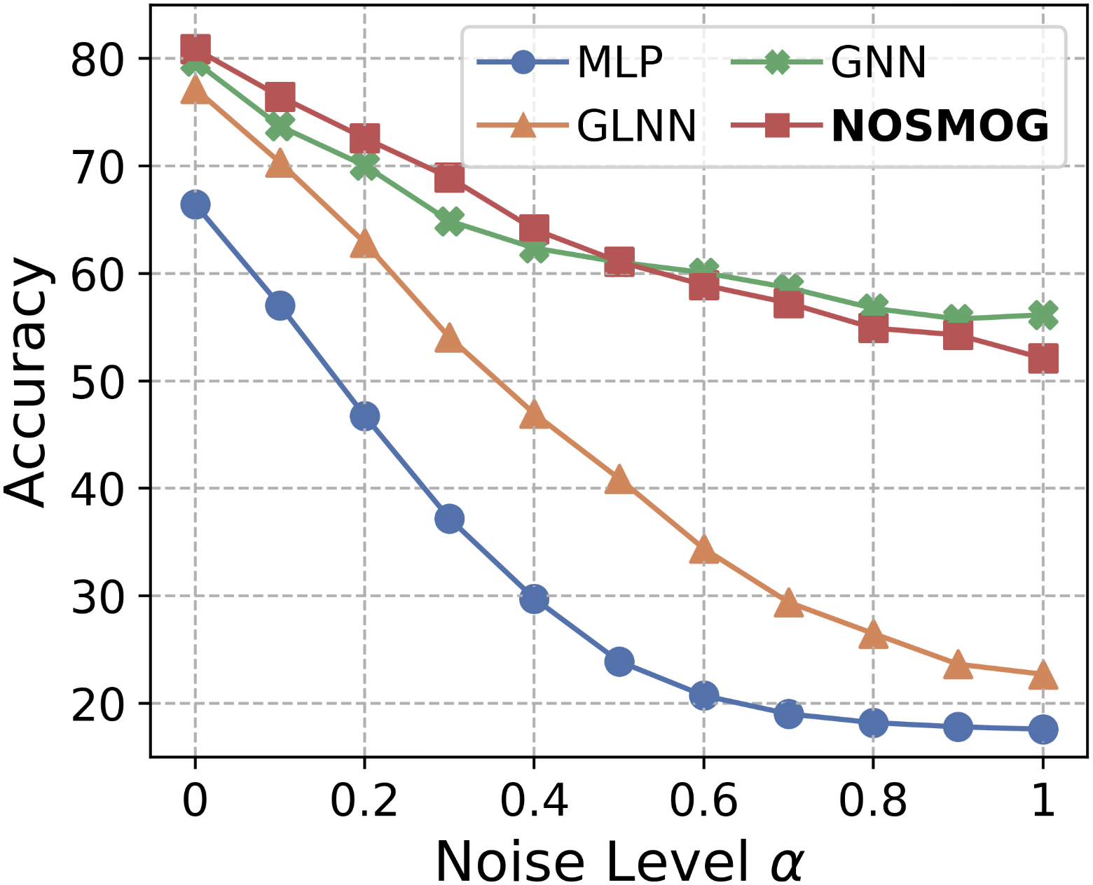
Figure 2: Accuracy vs. Feature Noises.

Considering that MLP and GLNN are sensitive to feature noises and may not perform well when the labels are uncorrelated with the node content, we further evaluate the performance of NOSMOG with regards to noise levels in Figure 2. Experiment results are averaged across various datasets. Specifically, we add different levels of Gaussian noises to content features by replacing ${\bm{C}}$ with $\tilde{{\bm{C}}}=(1-\alpha){\bm{C}}+\alpha n$, where $n$ represents Gaussian noises that independent from ${\bm{C}}$, and $\alpha\in[0,1]$ incates the noise level. We find that NOSMOG achieves better or comparable performance to GNNs across different $\alpha$, which demonstrates the superior efficacy of NOSMOG, especially when GNNs can mitigate the impact of noises by leveraging information from neighbors and surrounding subgraphs, whereas NOSMOG only relies on content and position features. GLNN and MLP, however, drop their performance quickly as $\alpha$ increases. In the extreme case when $\alpha$ equals 1, the input features are completely noises and $\tilde{\bm{C}}$ and ${\bm{C}}$ are independent. We observe that NOSMOG can still perform as good as GNNs by considering the position features, while GLNN and MLP perform poorly.

5.5 How does NOSMOG perform in terms of inference time?

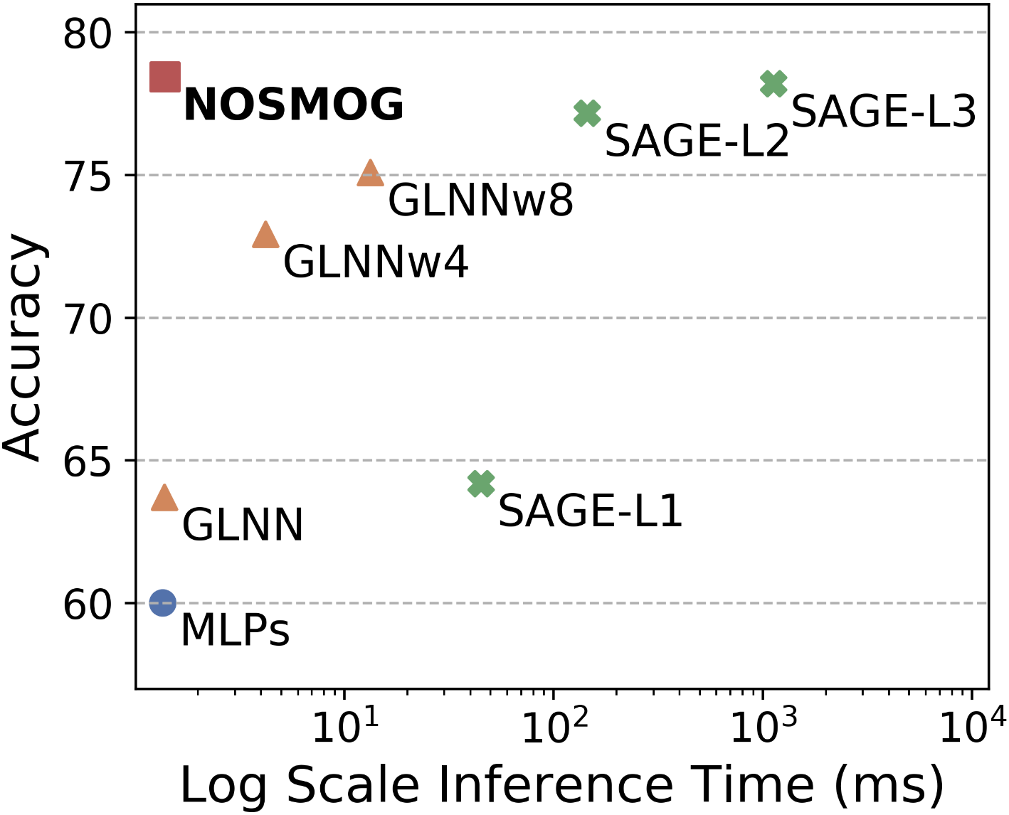
Figure 3: Accuracy vs. Inference Time.

To demonstrate the efficiency of NOSMOG, we analyze the capacity of NOSMOG by visualizing the trade-off between prediction accuracy and model inference time on Products dataset in Figure 3. We find that NOSMOG can achieve high accuracy (78%) while maintaining a fast inference time (1.35ms). Specifically, compared to other models with similar inference time, NOSMOG performs significantly better, while GLNN and MLPs can only achieve 64% and 60% accuracy, respectively. For those models that have close or similar performance as NOSMOG, they need a considerable amount of time for inference, e.g., 2 layers GraphSAGE (SAGE-L2) needs 144.47ms and 3 layers GraphSAGE (SAGE-L3) needs 1125.43ms, which is not applicable in real applications. This makes NOSMOG 107× faster than SAGE-L2 and 833× faster than SAGE-L3. In addition, since increasing the hidden size of GLNN may improve the performance, we compare NOSMOG with GLNNw4 (4-times wider than GLNN) and GLNNw8 (8-times wider than GLNN). Results show that although GLNNw4 and GLNNw8 can improve GLNN, they still perform worse than NOSMOG and even require more time for inference. We thus conclude that NOSMOG is superior to existing methods and GNNs in terms of both accuracy and inference time.

5.6 How does NOSMOG perform with different model components?

Table 3: Accuracy of different model variants. The decreasing performance of these model variants demonstrates the effectiveness of each component in enhancing the model.

Datasets w/o POS w/o RSD w/o ADV NOSMOG $\Delta_{POS}$ $\Delta_{RSD}$ $\Delta_{ADV}$ Cora 80.44 $\pm$ 1.51 82.11 $\pm$ 1.33 82.43 $\pm$ 1.42 83.04 $\pm$ 1.26 $\uparrow$ 3.23% $\uparrow$ 1.13% $\uparrow$ 0.74% Citeseer 73.31 $\pm$ 1.55 71.61 $\pm$ 1.84 72.11 $\pm$ 1.68 73.78 $\pm$ 1.54 $\uparrow$ 0.64% $\uparrow$ 3.03% $\uparrow$ 2.32% Pubmed 75.55 $\pm$ 2.54 77.15 $\pm$ 2.31 77.02 $\pm$ 2.58 77.34 $\pm$ 2.36 $\uparrow$ 2.37% $\uparrow$ 0.25% $\uparrow$ 0.42% A-computer 82.94 $\pm$ 0.87 84.00 $\pm$ 1.65 83.15 $\pm$ 1.21 84.04 $\pm$ 1.01 $\uparrow$ 1.33% $\uparrow$ 0.05% $\uparrow$ 1.07% A-photo 92.76 $\pm$ 0.58 92.97 $\pm$ 0.70 92.24 $\pm$ 0.98 93.36 $\pm$ 0.69 $\uparrow$ 0.65% $\uparrow$ 0.42% $\uparrow$ 1.21% Arxiv 62.69 $\pm$ 0.64 71.59 $\pm$ 0.27 71.53 $\pm$ 0.30 71.65 $\pm$ 0.29 $\uparrow$ 14.29% $\uparrow$ 0.08% $\uparrow$ 0.17% Products 63.75 $\pm$ 0.21 78.38 $\pm$ 0.36 78.35 $\pm$ 0.40 78.45 $\pm$ 0.38 $\uparrow$ 23.06% $\uparrow$ 0.09% $\uparrow$ 0.13%

Since NOSMOG contains various essential components (i.e., node position features (POS), representational similarity distillation (RSD), and adversarial feature augmentation (ADV)), we conduct ablation studies to analyze the contributions of different components by removing each of them independently (see Table 3). From the table, we find that the performance drops when a component is removed, indicating the efficiency of each component. In general, the incorporation of position features contributes the most, especially on Arxiv and Products datasets. By integrating the position features, NOSMOG can learn from the node positions and achieve exceptional performance. RSD contributes little to the overall performance across different datasets. This is because the goal of RSD is to distill more information from GNN to MLP, while MLP already learns well by mimicking GNN through soft labels. ADV contributes moderately across datasets, given that it mitigates overfitting and improves generalization. Finally, NOSMOG achieves the best performance on all datasets, demonstrating the effectiveness of the proposed model.

5.7 How does NOSMOG perform with different teacher GNNs?

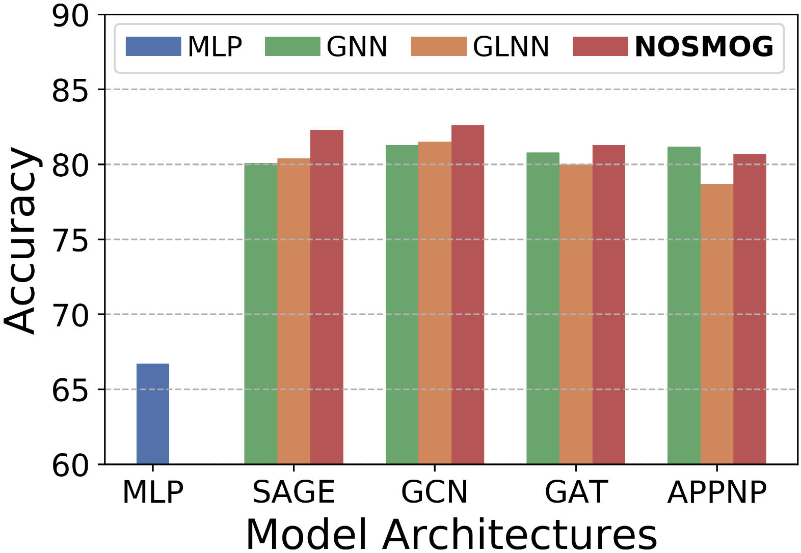
Figure 4: Accuracy vs. GNN Teacher Model Architectures.

We use GraphSAGE to represent the teacher GNNs so far. However, different GNN architectures may have different performances across datasets, we thus study if NOSMOG can perform well with other GNNs. In Figure 4, we show average performance with different teacher GNNs (i.e., GCN, GAT, and APPNP) across the five benchmark datasets. From the figure, we conclude that the performance of all four teachers is comparable, and NOSMOG can always learn from different teachers and outperform them, albeit with slightly diminished performance when distilled from APPNP, indicating that APPNP provides the least benefit for student. This is due to the fact that the APPNP uses node features for prediction prior to the message passing on the graph, which is very similar to what the student MLP does, and therefore provides MLP with little additional information than other teachers. However, NOSMOG consistently outperforms GLNN, which further demonstrates the effectiveness of the proposed model.

5.8 How can we explain the superior performance of NOSMOG?

In this section, we analyze the superior performance and expressiveness of NOSMOG from several perspectives, including the comparison with GLNN and GNNs from information theoretic perspective, and the consistency measure of model predictions and graph topology based on Min-Cut.

The expressiveness of NOSMOG compared to GLNN and GNNs. The goal of node classification task is to fit a function $f$ on the rooted graph ${\mathcal{G}}^{[v]}$ with label ${\bm{y}}_{v}$ (a rooted graph ${\mathcal{G}}^{[v]}$ is the graph with one node $v$ in ${\mathcal{G}}^{[v]}$ designated as the root) [2]. From the information theoretic perspective, learning $f$ by minimizing cross-entropy loss is equivalent to maximizing the mutual information (MI) [26], i.e., $I({\mathcal{G}}^{[v]};{\bm{y}}_{i})$. If we consider ${\mathcal{G}}^{[v]}$ as a joint distribution of two random variables ${\bm{X}}^{[v]}$ and $\mathcal{E}^{[v]}$, that represent the node features and edges in ${\mathcal{G}}^{[v]}$ respectively, we have: $I({\mathcal{G}}^{[v]};{\bm{y}}_{v})=I({\bm{X}}^{[v]},\mathcal{E}^{[v]};{\bm{y}}_{v})=I(\mathcal{E}^{[v]};{\bm{y}}_{v})+I({\bm{X}}^{[v]};{\bm{y}}_{v}|\mathcal{E}^{[v]})$, where $I(\mathcal{E}^{[v]};{\bm{y}}_{v})$ is the MI between edges and labels, which indicates the relevance between labels and graph structure, and $I({\bm{X}}^{[v]};{\bm{y}}_{v}|\mathcal{E}^{[v]})$ is the MI between features and labels given edges $\mathcal{E}^{[v]}$. To compare the effectiveness of NOSMOG, GLNN and GNNs, we start by analyzing the objective of GNNs. For a given node $v$, GNNs aim to learn an embedding function $f_{GNN}$ that computes the node embedding ${\bm{z}}_{v}$, where the objective is to maximize the likelihood of the conditional distribution $P({\bm{y}}_{v}|{\bm{z}}^{[v]})$ to approximate $I({\mathcal{G}}^{[v]};{\bm{y}}_{v})$. Generally, the embedding function $f_{GNN}$ takes the node features $X^{[v]}$ and its multi-hop neighbourhood subgraph $S^{[v]}$ as input, which can be written as ${\bm{z}}^{[v]}=f_{GNN}(X^{[v]},S^{[v]})$. Correspondingly, the process of maxmizing likelihood $P({\bm{y}}_{v}|{\bm{z}}^{[v]})$ can be expressed as the process of minimizing the objective function $\mathcal{L}_{1}(f_{GNN}(X^{[v]},S^{[v]}),{\bm{y}}_{v})$. Since $S^{[v]}$ contains the multi-hop neighbours, optimizing $\mathcal{L}_{1}$ captures both node features and the surrounding structure information, which approximating $I({\bm{X}}^{[v]};{\bm{y}}_{v}|\mathcal{E}^{[v]})$ and $I(\mathcal{E}^{[v]};{\bm{y}}_{v})$, respectively.

GLNN leverages the objective functions described in Eq. 1, which approximates $I({\mathcal{G}}^{[v]};{\bm{y}}_{v})$ by only maxmizing $I({\bm{X}}^{[v]};{\bm{y}}_{v}|\mathcal{E}^{[v]})$, while ignoring $I(\mathcal{E}^{[v]};{\bm{y}}_{v})$. However, there are situations that node labels are not strongly correlated to node features, or labels are mainly determined by the node positions or graph structure, e.g., node degrees [21, 47]. In these cases, GLNN won’t be able to fit. Alternatively, NOSMOG focuses on modeling both $I(\mathcal{E}^{[v]};{\bm{y}}_{v})$ and $I({\bm{X}}^{[v]};{\bm{y}}_{v}|\mathcal{E}^{[v]})$ by jointly considering node position features and content features. In particular, $I(\mathcal{E}^{[v]};{\bm{y}}_{v})$ is optimized by the objective functions $\mathcal{L}_{2}(f_{MLP}(X^{[v]},P^{[v]}),{\bm{y}}_{v})$ and $\mathcal{L}_{3}(f_{MLP}(X^{[v]},P^{[v]}),f_{GNN}(X^{[v]},S^{[v]}))$ by extending $\mathcal{L}_{GT}$ and $\mathcal{L}_{SL}$ in Equation 8 that incorporates position features. Here $f_{MLP}$ is the embedding function that NOSMOG learns given the content feature $X^{[v]}$ and position feature $P^{[v]}$. Essentially, optimizing $\mathcal{L}_{3}$ forces MLP to learn from GNN’s output and eventually achieve comparable performance as GNNs. In the meanwhile, optimizing $\mathcal{L}_{2}$ allows MLP to capture node positions that may not be learned by GNNs, which is important if the label ${\bm{y}}_{v}$ is correlated to the node positional information. Therefore, there is no doubt that NOSMOG can perform better, considering that ${\bm{y}}_{v}$ is always correlated with $\mathcal{E}^{[v]}$ in graph data. Even in the extreme case that when ${\bm{y}}_{v}$ is uncorrelated with $I({\bm{X}}^{[v]};{\bm{y}}_{v}|\mathcal{E}^{[v]})$, NOSMOG can still achieve superior or comparable performance to GNNs, as demonstrated in Section 5.4.

Table 4: The cut value. NOSMOG predictions are more consistent with the graph topology than GNN, MLP, and the state-of-the-art method GLNN.

Datasets SAGE MLP GLNN NOSMOG Cora 0.9385 0.7203 0.8908 0.9480 Citeseer 0.9535 0.8107 0.9447 0.9659 Pubmed 0.9597 0.9062 0.9298 0.9641 A-computer 0.8951 0.6764 0.8579 0.9047 A-photo 0.9014 0.7099 0.9063 0.9084 Arxiv 0.9052 0.7252 0.8126 0.9066 Products 0.9400 0.7518 0.7657 0.9456 Average 0.9276 0.7572 0.8725 0.9348

The consistency measure of model predictions and graph topology. To further validate that NOSMOG is superior to GNNs, MLPs, and GLNN in encoding graph structural information, we design the cut value $\mathcal{CV}\in[0,1]$ to measure the consistency between model predictions and graph topology [44], based on the approximation for the min-cut problem [1]. The min-cut problem divides nodes $\mathcal{V}$ into $K$ disjoint subsets by removing the minimum number of edges. Correspondingly, the min-cut problem can be expressed as: $\max\frac{1}{K}\sum_{k=1}^{K}({\bm{C}}^{T}_{k}{\bm{A}}{\bm{C}}_{k})/({\bm{C}}^{T}_{k}{\bm{D}}{\bm{C}}_{k})$, where ${\bm{C}}$ is the node class assignment, ${\bm{A}}$ is the adjacency matrix, and ${\bm{D}}$ is the degree matrix. Therefore, we design the cut value as follows: $\mathcal{CV}=tr(\hat{\bm{Y}}^{T}{\bm{A}}\hat{\bm{Y}})/tr(\hat{\bm{Y}}^{T}{\bm{D}}\hat{\bm{Y}})$, where $\hat{\bm{Y}}$ is the model prediction output, and the cut value $\mathcal{CV}$ indicates the consistency between the model predictions and the graph topology. The bigger the value is, the predictions are more consistent with the graph topology, and the model is more capable of capturing graph structural information. The cut values for different models in transductive setting are shown in Table 4. We find that the average $\mathcal{CV}$ for NOSMOG is 0.9348, while the average $\mathcal{CV}$ for SAGE, MLP, and GLNN are 0.9276, 0.7572, and 0.8725, respectively. We conclude that NOSMOG achieves the highest cut value, demonstrating the superior expressiveness of NOSMOG in capturing graph topology compared to GNN, MLP, and GLNN.

6 Conclusion

In this paper, we address two issues that the existing GNNs-MLPs framework has, i.e., the ignorance of graph structural information and the sensitivity to node feature noises. Specifically, we propose to learn Noise-robust and Structure-aware MLPs on Graphs (NOSMOG) that considers position features, representational similarity distillation, and adversarial feature augmentation. Extensive experiments on seven datasets demonstrate that NOSMOG can improve GNNs by 2.05%, MLPs by 25.22%, and the state-of-the-art method by 6.63%, meanwhile maintaining a fast inference speed of 833× compared to GNNs. In addition, we present robustness analysis, efficiency comparison, ablation studies, and theoretical explanation to better understand the effectiveness of the proposed model.

References

- [1] Filippo Maria Bianchi, Daniele Grattarola, and Cesare Alippi. Mincut pooling in graph neural networks. arXiv preprint arXiv:1907.00481, 2019.
- [2] Lei Chen, Zhengdao Chen, and Joan Bruna. On graph neural networks versus graph-augmented mlps. In ICLR, 2021.
- [3] Ming Chen, Zhewei Wei, Zengfeng Huang, Bolin Ding, and Yaliang Li. Simple and deep graph convolutional networks. In ICML, 2020.
- [4] Tianlong Chen, Yu Cheng, Zhe Gan, Jianfeng Wang, Lijuan Wang, Zhangyang Wang, and Jingjing Liu. Adversarial feature augmentation and normalization for visual recognition. arXiv preprint arXiv:2103.12171, 2021.
- [5] Zhijie Deng, Yinpeng Dong, and Jun Zhu. Batch virtual adversarial training for graph convolutional networks. arXiv preprint arXiv:1902.09192, 2019.
- [6] Prasenjit Dey, Kaustuv Nag, Tandra Pal, and Nikhil R Pal. Regularizing multilayer perceptron for robustness. IEEE Transactions on Systems, Man, and Cybernetics: Systems, 2017.
- [7] Jianping Gou, Baosheng Yu, Stephen J Maybank, and Dacheng Tao. Knowledge distillation: A survey. International Journal of Computer Vision, 2021.
- [8] Zhichun Guo, Chunhui Zhang, Yujie Fan, Yijun Tian, Chuxu Zhang, and Nitesh Chawla. Boosting graph neural networks via adaptive knowledge distillation. In AAAI, 2023.
- [9] William L. Hamilton, Rex Ying, and Jure Leskovec. Inductive representation learning on large graphs. In NeurIPS, 2017.
- [10] Geoffrey Hinton, Oriol Vinyals, Jeff Dean, et al. Distilling the knowledge in a neural network. arXiv preprint arXiv:1503.02531, 2015.
- [11] Weihua Hu, Matthias Fey, Marinka Zitnik, Yuxiao Dong, Hongyu Ren, Bowen Liu, Michele Catasta, and Jure Leskovec. Open graph benchmark: Datasets for machine learning on graphs. In NeurIPS, 2020.
- [12] Yang Hu, Haoxuan You, Zhecan Wang, Zhicheng Wang, Erjin Zhou, and Yue Gao. Graph-mlp: node classification without message passing in graph. arXiv preprint arXiv:2106.04051, 2021.
- [13] Zhihao Jia, Sina Lin, Rex Ying, Jiaxuan You, Jure Leskovec, and Alex Aiken. Redundancy-free computation for graph neural networks. In KDD, 2020.
- [14] Ziyu Jiang, Tianlong Chen, Ting Chen, and Zhangyang Wang. Robust pre-training by adversarial contrastive learning. In NeurIPS, 2020.
- [15] Thomas N. Kipf and Max Welling. Semi-supervised classification with graph convolutional networks. In ICLR, 2017.
- [16] Johannes Klicpera, Aleksandar Bojchevski, and Stephan Günnemann. Predict then propagate: Graph neural networks meet personalized pagerank. In ICLR, 2019.
- [17] Kezhi Kong, Guohao Li, Mucong Ding, Zuxuan Wu, Chen Zhu, Bernard Ghanem, Gavin Taylor, and Tom Goldstein. Flag: Adversarial data augmentation for graph neural networks. In CVPR, 2022.
- [18] Seunghyun Lee and Byung Cheol Song. Graph-based knowledge distillation by multi-head attention network. arXiv preprint arXiv:1907.02226, 2019.
- [19] Guohao Li, Matthias Muller, Ali Thabet, and Bernard Ghanem. Deepgcns: Can gcns go as deep as cnns? In ICCV, 2019.
- [20] Pan Li, Yanbang Wang, Hongwei Wang, and Jure Leskovec. Distance encoding: Design provably more powerful neural networks for graph representation learning. In NeurIPS, 2020.
- [21] Derek Lim, Xiuyu Li, Felix Hohne, and Ser-Nam Lim. New benchmarks for learning on non-homophilous graphs. In WWW, 2021.
- [22] Aleksander Madry, Aleksandar Makelov, Ludwig Schmidt, Dimitris Tsipras, and Adrian Vladu. Towards deep learning models resistant to adversarial attacks. In ICLR, 2018.
- [23] Christopher Morris, Martin Ritzert, Matthias Fey, William L Hamilton, Jan Eric Lenssen, Gaurav Rattan, and Martin Grohe. Weisfeiler and leman go neural: Higher-order graph neural networks. In AAAI, 2019.
- [24] Bryan Perozzi, Rami Al-Rfou, and Steven Skiena. Deepwalk: Online learning of social representations. In KDD, 2014.
- [25] Mary Phuong and Christoph Lampert. Towards understanding knowledge distillation. In ICML, 2019.
- [26] Zhenyue Qin, Dongwoo Kim, and Tom Gedeon. Rethinking softmax with cross-entropy: Neural network classifier as mutual information estimator. arXiv preprint arXiv:1911.10688, 2019.
- [27] Yijun Tian, Kaiwen Dong, Chunhui Zhang, Chuxu Zhang, and Nitesh V Chawla. Heterogeneous graph masked autoencoders. In AAAI, 2023.
- [28] Yijun Tian, Shichao Pei, Xiangliang Zhang, Chuxu Zhang, and Nitesh V Chawla. Knowledge distillation on graphs: A survey. arXiv preprint arXiv:2302.00219, 2023.
- [29] Yijun Tian, Chuxu Zhang, Zhichun Guo, Yihong Ma, Ronald Metoyer, and Nitesh V Chawla. Recipe2vec: Multi-modal recipe representation learning with graph neural networks. In IJCAI, 2022.
- [30] Frederick Tung and Greg Mori. Similarity-preserving knowledge distillation. In ICCV, 2019.
- [31] Petar Veličković, Guillem Cucurull, Arantxa Casanova, Adriana Romero, Pietro Liò, and Yoshua Bengio. Graph attention networks. In ICLR, 2018.
- [32] Dilin Wang, Chengyue Gong, and Qiang Liu. Improving neural language modeling via adversarial training. In ICML, 2019.
- [33] Haorui Wang, Haoteng Yin, Muhan Zhang, and Pan Li. Equivariant and stable positional encoding for more powerful graph neural networks. In ICLR, 2022.
- [34] Zonghan Wu, Shirui Pan, Fengwen Chen, Guodong Long, Chengqi Zhang, and S Yu Philip. A comprehensive survey on graph neural networks. IEEE transactions on neural networks and learning systems, 2020.
- [35] Cihang Xie, Mingxing Tan, Boqing Gong, Jiang Wang, Alan L Yuille, and Quoc V Le. Adversarial examples improve image recognition. In CVPR, 2020.
- [36] Keyulu Xu, Weihua Hu, Jure Leskovec, and Stefanie Jegelka. How powerful are graph neural networks? In ICLR, 2019.
- [37] Bencheng Yan, Chaokun Wang, Gaoyang Guo, and Yunkai Lou. Tinygnn: Learning efficient graph neural networks. In KDD, 2020.
- [38] Cheng Yang, Jiawei Liu, and Chuan Shi. Extract the knowledge of graph neural networks and go beyond it: An effective knowledge distillation framework. In WWW, 2021.
- [39] Yiding Yang, Jiayan Qiu, Mingli Song, Dacheng Tao, and Xinchao Wang. Distilling knowledge from graph convolutional networks. In CVPR, 2020.
- [40] Jiaxuan You, Rex Ying, and Jure Leskovec. Position-aware graph neural networks. In ICML, 2019.
- [41] Chunhui Zhang, Chao Huang, Yijun Tian, Qianlong Wen, Zhongyu Ouyang, Youhuan Li, Yanfang Ye, and Chuxu Zhang. Diving into unified data-model sparsity for class-imbalanced graph representation learning. In GLFrontiers, 2022.
- [42] Chunhui Zhang, Yijun Tian, Mingxuan Ju, Zheyuan Liu, Yanfang Ye, Nitesh Chawla, and Chuxu Zhang. Chasing all-round graph representation robustness: Model, training, and optimization. In ICLR, 2023.
- [43] Dalong Zhang, Xin Huang, Ziqi Liu, Zhiyang Hu, Xianzheng Song, Zhibang Ge, Zhiqiang Zhang, Lin Wang, Jun Zhou, Yang Shuang, et al. Agl: A scalable system for industrial-purpose graph machine learning. arXiv preprint arXiv:2003.02454, 2020.
- [44] Shichang Zhang, Yozen Liu, Yizhou Sun, and Neil Shah. Graph-less neural networks: Teaching old mlps new tricks via distillation. In ICLR, 2022.
- [45] Wenqing Zheng, Edward W Huang, Nikhil Rao, Sumeet Katariya, Zhangyang Wang, and Karthik Subbian. Cold brew: Distilling graph node representations with incomplete or missing neighborhoods. In ICLR, 2022.
- [46] Jie Zhou, Ganqu Cui, Shengding Hu, Zhengyan Zhang, Cheng Yang, Zhiyuan Liu, Lifeng Wang, Changcheng Li, and Maosong Sun. Graph neural networks: A review of methods and applications. AI Open, 2020.
- [47] Jiong Zhu, Ryan A Rossi, Anup Rao, Tung Mai, Nedim Lipka, Nesreen K Ahmed, and Danai Koutra. Graph neural networks with heterophily. In AAAI, 2021.
- [48] Daniel Zügner, Amir Akbarnejad, and Stephan Günnemann. Adversarial attacks on neural networks for graph data. In KDD, 2018.