M/D/1 Queues with LIFO and SIRO Policies

Abstract

While symbolics for the equilibrium M/D/1-LIFO waiting time density are completely known, corresponding numerics for M/D/1-SIRO are derived from recursions due to Burke (1959).  Implementing an inverse Laplace transform-based approach for the latter remains unworkable.

We examined in [1] a first-in-first-out M/D/1 queue alongside unlimited waiting space, where the input process is Poisson with rate $\lambda$ and the service times are constant with value $1/\mu=a$.  The FIFO policy of sorting clients, which is plainly fair and has minimal waiting time variance [2], is also known as FCFS: first-come-first-serve.

Keeping all other features the same, we wonder about the effect of replacing FIFO by LIFO: last-in-first-out. This policy, which seems patently unfair and has maximal waiting time variance [3], is also known as LCFS: last-come-first-serve.

Intermediate to FIFO and LIFO is SIRO: serve-in-random-order.  This policy is variously known as ROS: random-order-of-service and RSS: random-selection-for-service.  Analysis of SIRO is more difficult than that of LIFO, as will be seen.

1 LIFO

Let $W_{\text{que}}$ denote the waiting time in the queue (prior to service).  Under equilibrium (steady-state) conditions and traffic intensity (load) $\rho=\lambda/\mu<1$, the probability density function $f(x)$ of $W_{\text{que}}$ has Laplace transform [4, 5, 6, 7]

$$F(s)=\lim_{\varepsilon\rightarrow 0^{+}}{\displaystyle\int\limits_{-\varepsilon}^{\infty}}\exp(-s\,x)f(x)dx=1-\rho+\frac{\lambda-\lambda\,\Theta(s)}{s+\lambda-\lambda\,\Theta(s)}=F_{\text{alt}}(s)+1-\rho$$

where

$$\begin{array}[c]{ccc}\theta(x)={\displaystyle\sum\limits_{k=1}^{\infty}}e^{-k\,\rho}\dfrac{(k\,\rho)^{k-1}}{k!}\delta(x-a\,k),&&\Theta(s)=-\dfrac{1}{\rho}\,\omega\left(-\rho\exp\left(-\rho-a\,s\right)\right),\end{array}$$

$\delta(x)$ is the Dirac delta and $\omega(s)$ is the principal branch of the Lambert omega:

$$\begin{array}[c]{ccccc}\omega(s)e^{\omega(s)}=s,&&-1\leq\omega(x)\in\mathbb{R}\text{ \ }\forall\text{ }x\geq-1/e,&&\exists\text{ branch cut for }x<-1/e.\end{array}$$

From

$$(1-\rho)s+\lambda\,\left[1-\Theta(s)\right](1-\rho+1)=s\,F(s)+\lambda\,F(s)\left[1-\Theta(s)\right]$$

we have

$$(1-\rho)s+\lambda\left(2-\rho-F(s)\right)\left[1-\Theta(s)\right]=s\,F(s),$$

i.e.,

$$F(s)=1-\rho+\lambda\left(2-\rho-F(s)\right)\left[\frac{1}{s}-\frac{\Theta(s)}{s}\right]$$

hence

$$f(x) =(1-\rho)\delta(x)+\kappa+\lambda{\displaystyle\int\limits_{0}^{x}}\left((2-\rho)\delta(t)-f(t)\right)\left[1-{\displaystyle\int\limits_{0}^{x-t}}\theta(u)du\right]dt$$

$$=(1-\rho)\delta(x)+\lambda+\lambda(2-\rho)\left[1-{\displaystyle\int\limits_{0}^{x}}\theta(u)du\right]-\lambda{\displaystyle\int\limits_{0}^{x}}f(t)\left[1-{\displaystyle\int\limits_{0}^{x-t}}\theta(u)du\right]dt.$$

The indicated condition $\kappa=\lambda$ is true by the initial value theorem [8]:

$$\lim_{\varepsilon\rightarrow 0^{+}}f(\varepsilon)=\lim\limits_{s\rightarrow 1\cdot\infty}s\,F_{\text{alt}}(s).$$

Differentiating, we obtain

$$f^{\prime}(x) =\lambda(2-\rho)\left[0-\theta(x)\right]-\lambda f(x)\left[1-0\right]-\lambda{\displaystyle\int\limits_{0}^{x}}f(t)\left[0-\theta(x-t)\right]dt$$

$$=-\lambda(2-\rho)\theta(x)-\lambda f(x)+\lambda{\displaystyle\int\limits_{0}^{x}}f(t)\theta(x-t)dt$$

$$=-\lambda(2-\rho)\theta(x)-\lambda f(x)+\lambda{\displaystyle\int\limits_{0}^{x}}f(t){\displaystyle\sum\limits_{k=1}^{\infty}}e^{-k\,\rho}\dfrac{(k\,\rho)^{k-1}}{k!}\delta(x-t-a\,k)dt$$

$$=-\lambda(2-\rho)\theta(x)-\lambda f(x)+\lambda{\displaystyle\sum\limits_{k=1}^{\infty}}e^{-k\,\rho}\dfrac{(k\,\rho)^{k-1}}{k!}{\displaystyle\int\limits_{0}^{x}}f(t)\delta(x-t-a\,k)dt$$

$$=-\lambda(2-\rho)\theta(x)-\lambda f(x)+\lambda{\displaystyle\sum\limits_{k=1}^{\infty}}e^{-k\,\rho}\dfrac{(k\,\rho)^{k-1}}{k!}f(x-a\,k).$$

For $0<x<a$,

$$\begin{array}[c]{ccc}f^{\prime}(x)=-\lambda\,f(x),&&f(0^{+})=\lambda\end{array}$$

implies

$$f(x)=\lambda\,e^{-\lambda\,x}.$$

Note that $\lim_{\varepsilon\rightarrow 0^{+}}f(a\,k+\varepsilon)=0$ for each $k\geq 1$ because, if a client arrives at the same moment the server becomes available, the client is taken immediately (by LIFO) and there is no waiting. For $a<x<2a$,

$$f^{\prime}(x) =-\lambda\,f(x)+\lambda\,e^{-\rho}\cdot\lambda\,e^{-\lambda(x-a)}$$

$$=-\lambda\,f(x)+\lambda^{2}e^{-\lambda\,x}$$

coupled with $f(a^{+})=0$ implies

$$f(x)=\lambda^{2}(x-a)e^{-\lambda\,x}.$$

For $2a<x<3a$,

$$f^{\prime}(x) =-\lambda\,f(x)+\lambda\,e^{-\rho}\cdot\lambda^{2}(x-2a)e^{-\lambda(x-a)}+\lambda\,e^{-2\rho}\frac{2\rho}{2!}\cdot\lambda\,e^{-\lambda(x-2a)}$$

$$=-\lambda\,f(x)+\lambda^{3}(x-a)e^{-\lambda\,x}$$

coupled with $f(2a^{+})=0$ implies

$$f(x)=\frac{1}{2}\lambda^{3}x(x-2a)e^{-\lambda\,x}.$$

For $3a<x<4a$,

$$f^{\prime}(x) =-\lambda\,f(x)+\lambda\,e^{-\rho}\cdot\frac{1}{2}\lambda^{3}(x-a)(x-3a)e^{-\lambda(x-a)}$$

$$+\lambda\,e^{-2\rho}\frac{2\rho}{2!}\cdot\lambda^{2}(x-3a)e^{-\lambda(x-2a)}+\lambda\,e^{-3\rho}\frac{(3\rho)^{2}}{3!}\cdot\lambda\,e^{-\lambda(x-3a)}$$

$$=-\lambda\,f(x)+\frac{1}{2}\lambda^{4}x(x-2a)e^{-\lambda\,x}$$

coupled with $f(3a^{+})=0$ implies

$$f(x)=\frac{1}{6}\lambda^{4}x^{2}(x-3a)e^{-\lambda\,x}.$$

More generally, for $k\,a<x<(k+1)a$, we obtain

$$f(x)=\frac{1}{k!}\lambda^{k+1}x^{k-1}(x-k\,a)e^{-\lambda\,x}$$

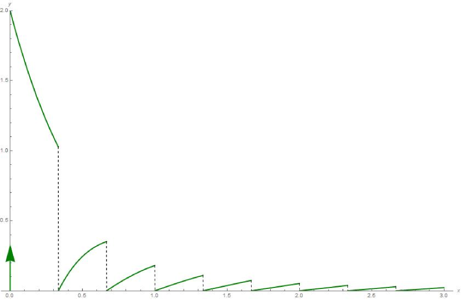
Figure 1: Waiting time density plot $y=f(x)$ for Deterministic[$\frac{1}{3}$] last-in-first-out service.

and thus the waiting time density for LIFO is completely understood.  Prabhu [9] and Peters [10] evidently hold priority in discovering this formula, the latter correcting an error in [11]. The density for M/D/1-FIFO is likewise completely understood [12] – no surprises occur here – although it is M/U/1-FIFO densities which are only effectively known [1].  Stitching the fragments together gives the LIFO density function pictured in Figure 1, for parameter values $\lambda=2$ and $\mu=3$; hence $\rho=2/3$ and $a=1/3$.  It is interesting to compare this plot with Figure 3 of [1], the FIFO density for identical parameter values.

Let $\xi=a^{2}$ and $\eta=a^{3}$.  Moments of $W_{\text{que}}$ for LIFO are [13, 14]

$$\begin{array}[c]{ccc}\text{mean}=-F^{\prime}(0)=\dfrac{\lambda\,\xi}{2(1-\rho)},&&\text{variance}=F^{\prime\prime}(0)-F^{\prime}(0)^{2}=\dfrac{\lambda\,\eta}{3(1-\rho)^{2}}+\dfrac{\lambda^{2}\xi^{2}(1+\rho)}{4(1-\rho)^{3}}\end{array}$$

giving $\frac{1}{3}$ and $\frac{7}{9}$ respectively.  The mean of $W_{\text{que}}$ for FIFO is the same as that for LIFO; the corresponding variance is smaller:

$$\begin{array}[c]{c}\dfrac{\lambda\,\eta}{3(1-\rho)}+\dfrac{\lambda^{2}\xi^{2}}{4(1-\rho)^{2}}\end{array}$$

giving $\frac{5}{27}$.  ($\xi$ and $\eta$ are second and third service time moments, used for consistency with earlier work.)

We clarify that, while $\theta(x)$ is the notation for service time density in [1], $\theta(x)$ here is the notation for busy period length density.  The probability that {a busy period $X$ is of length exactly $k\,a$} is equal to the probability that {exactly $k$ clients of a queue, having precisely $1$ starting client and traffic intensity $\rho$, are served before the queue first vanishes}.  This is known as the Borel distribution [15, 16, 17], which satisfies [18, 19, 20]

$$\mathbb{E}\left(\exp\left(-s\,\frac{X}{a}\right)\right)=-\dfrac{1}{\rho}\,\omega\left(-\rho\exp\left(-\rho-s\right)\right)$$

for M/D/1; thus the formula for $\Theta(s)=\mathbb{E}\left(\exp\left(-s\,X\right)\right)$ follows.

Study of busy period lengths is possible for M/U/1 – the density involves modified Bessel functions of the first kind [21] – it is far more complicated than the density for M/D/1.

2 SIRO

The probability density function $f(x)$ of $W_{\text{que}}$ has Laplace transform [22, 23, 24, 25]

$$F(s)=1+\frac{\lambda(1-\rho)}{s}{\displaystyle\int\limits_{\Theta(s)}^{1}}\Phi(s,z)\Psi(s,z)dz=F_{\text{alt}}(s)+1-\rho$$

where

$$\Phi(s,z)=\frac{1-z-a\,s/(1-\rho)}{z-e^{-a\,s-\rho(1-z)}}-\frac{1-z}{z-e^{-\rho(1-z)}},$$

$$\Psi(s,z)=\exp\left(-{\displaystyle\int\limits_{z}^{1}}\frac{dy}{y-e^{-a\,s-\rho(1-y)}}\right).$$

The integral underlying $\Psi(s,z)$ is intractable; our symbolic approach for FIFO & LIFO seems inapplicable for SIRO.

We therefore turn to a numeric approach developed by Burke [26], which is based on certain simplifying properties of M/D/1 that do not easily generalize.  Since $\mu=1$ is assumed in [26], we take $\lambda=2/3$ and rescale at the end.  Two recursions are key:

$$P_{n}=P_{n-1}e^{\lambda}-(P_{0}+P_{1})\frac{\lambda^{n-1}}{(n-1)!}-{\displaystyle\sum\limits_{j=2}^{n-1}}P_{j}\frac{\lambda^{n-j}}{(n-j)!},$$

$$\begin{array}[c]{ccc}P_{0}=1-\lambda,&&P_{1}=P_{0}e^{\lambda}-P_{0}\end{array}$$

where the empty sum convention holds for $n=2$, and

$$Q_{i}(n,m)=\left\{\begin{array}[c]{lll}\left(1-\dfrac{1}{n}\right)e^{-\lambda}\,{\displaystyle\sum\limits_{k=0}^{m}}\,\dfrac{\lambda^{k}}{k!}\,Q_{i-1}(n+k-1,m)&&\text{if }n>0,\\ 0&&\text{otherwise;}\end{array}\right.$$

$$\begin{array}[c]{ccc}Q_{i}(1,m)=\delta_{i},&&Q_{0}(n,m)=\left\{\begin{array}[c]{lll}\dfrac{1}{n}&\vskip 3.0pt plus 1.0pt minus 1.0pt&\text{if }n>0,\\ 0&&\text{otherwise}\end{array}\right.\end{array}$$

where $\delta_{i}$ is the Kronecker delta and $m$ is suitably large.  These lead to the probability that waiting time is $\leq t$:

$$H(t,m)=(1-\lambda)+\lambda\,{\displaystyle\sum\limits_{n=1}^{\infty}}P_{n-1}\cdot\left[\left(t-\left\lfloor t\right\rfloor\right)Q_{\left\lfloor t\right\rfloor}(n,m)+{\displaystyle\sum\limits_{i=0}^{\left\lfloor t\right\rfloor-1}}Q_{i}(n,m)\right]$$

in the limit as $m\rightarrow\infty$, where again the empty sum convention holds for $0\leq t<1$.

Clearly the preceding expression simplifies to

$$(1-\lambda)+\lambda\,t\,{\displaystyle\sum\limits_{n=1}^{\infty}}\frac{P_{n-1}}{n}$$

for all $0\leq t\leq 1$ and any $m\geq 0$.  The dependence of $H(t,m)$ on $m$ becomes visible for $t>1$.  To find the waiting time density value, let $t^{\prime}=t+\frac{1}{4}$ (an arbitrary choice) and assume $0<t<t^{\prime}<1$.  Then

$$4\left(H(t^{\prime},m)-H(t,m)\right)=\lambda\,{\displaystyle\sum\limits_{n=1}^{\infty}}\frac{P_{n-1}}{n}$$

and, rescaling,

$$12\left(H(t^{\prime},m)-H(t,m)\right)=2\,{\displaystyle\sum\limits_{n=1}^{\infty}}\frac{P_{n-1}}{n}=1.176773....$$

This corresponds to the height of the leftmost rectangle in Figure 2, surmounting the interval $[0,\frac{1}{3}]$.

For $1<t<t^{\prime}<2$, the rescaled density value is

$$\lim_{m\rightarrow\infty}\,12\left(H(t^{\prime},m)-H(t,m)\right) =2\,{\displaystyle\sum\limits_{n=2}^{\infty}}P_{n-1}\left(1-\dfrac{1}{n}\right)e^{-\lambda}\,{\displaystyle\sum\limits_{k=0}^{\infty}}\,\dfrac{\lambda^{k}}{k!}\,\frac{1}{n+k-1}$$

$$=0.392099...$$

which corresponds to the height of the rectangle surmounting the interval $[\frac{1}{3},\frac{2}{3}]$.  Unlike earlier, the requirement that $m$ is large becomes essential.  For $2<t<t^{\prime}<3$, the formula for $Q_{2}(n,m)$ involving $\{Q_{0}(n,m),Q_{1}(n,m)\}$ is more complicated than that for $Q_{1}(n,m)$.  It is better to implement the recursion than to write the formula.  Summarizing, initial segments of the sought-after density function are

$$g(x)=\left\{\begin{array}[c]{lll}c_{1}=1.176773...&&\text{if }0<x<\frac{1}{3},\\ c_{2}=0.392099...&&\text{if }\frac{1}{3}<x<\frac{2}{3},\\ c_{3}=0.179926...&&\text{if }\frac{2}{3}<x<1,\\ c_{4}=0.095228...&&\text{if }1<x<\frac{4}{3},\\ c_{5}=0.054829...&&\text{if }\frac{4}{3}<x<\frac{5}{3},\\ c_{6}=0.033415...&&\text{if }\frac{5}{3}<x<2,\\ c_{7}=0.021228...&&\text{if }2<x<\frac{7}{3},\\ c_{8}=0.013923...&&\text{if }\frac{7}{3}<x<\frac{8}{3},\\ c_{9}=0.009369...&&\text{if }\frac{8}{3}<x<3.\end{array}\right.$$

The Laplace transform of $g(x)$ is

$$G(s)={\displaystyle\sum\limits_{j=1}^{\infty}}c_{j}\frac{\exp\left(-\frac{j-1}{3}s\right)-\exp\left(-\frac{j}{3}s\right)}{s}$$

and verification that $G(s)=F_{\text{alt}}(s)$ can be done experimentally (although not yet theoretically).

We wonder about possible generalizations of this approach: works that cite [26] include [27, 28, 29].  It is known (by other techniques) that the mean of $W_{\text{que}}$ for SIRO is the same as that for FIFO and LIFO; the corresponding variance is between the two extremes [30, 31, 32]:

$$\dfrac{2\,\lambda\,\eta}{3(1-\rho)(2-\rho)}+\dfrac{\lambda^{2}\xi^{2}(2+\rho)}{4(1-\rho)^{2}(2-\rho)}$$

giving $\frac{1}{3}$.

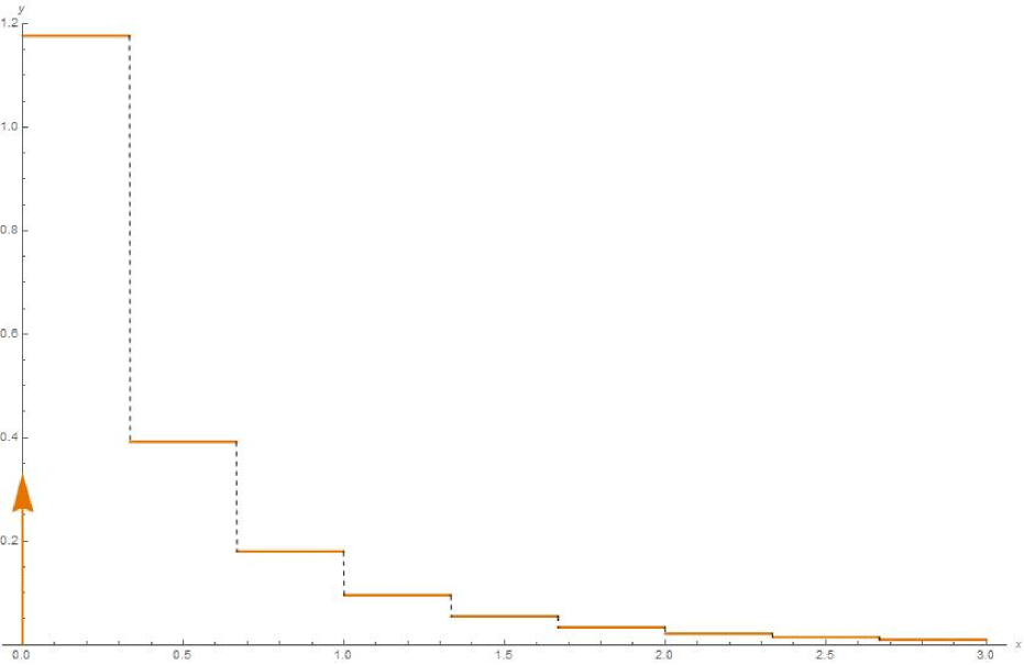
Figure 2: Waiting time density plot $y=g(x)$ for Deterministic[$\frac{1}{3}$] serve-in-random-order policy.

3 Addendum

Let us briefly summarize corresponding results for M/M/1.  For LIFO, the density $f(x)$ for $W_{\text{que}}$ is [11, 33, 34, 35]

$$f(x)=(1-\rho)\delta(x)+\sqrt{\frac{\mu}{\lambda}}\,\frac{\exp\left[-(\lambda+\mu)x\right]\,I_{1}\left(2\sqrt{\lambda\,\mu}\,x\right)}{x}$$

where $I_{1}(\cdot)$ is the modified Bessel function of first order.  Since $\xi=2/\mu^{2}$ and $\eta=6/\mu^{3}$, the mean and variance are $\frac{2}{3}$ and $\frac{32}{9}$ respectively for parameter values $\lambda=2$ and $\mu=3$.  Note that $\frac{32}{9}>\frac{8}{9}$, which is the analogous variance for FIFO.

For SIRO, the density $f(x)$ for $W_{\text{que}}$ is likewise of the form $(1-\rho)\delta(x)+\varphi(x)$ where [36, 37]

$$\varphi(x)=2(\mu-\lambda){\displaystyle\int\limits_{0}^{\pi}}\,\frac{\exp\left[\left(2\psi(\tau)-\tau\right)\cot(\tau)\right]}{\exp\left[\pi\cot(\tau)\right]+1}\,\frac{\exp\left[-\lambda\left(1-\frac{2}{\sqrt{\rho}}\cos(\tau)+\frac{1}{\rho}\right)x\right]}{1-\frac{2}{\sqrt{\rho}}\cos(\tau)+\frac{1}{\rho}}\sin(\tau)d\tau$$

and

$$\psi(\tau)=\left\{\begin{array}[c]{lll}\arctan\left(\dfrac{\sin(\tau)}{\cos(\tau)-\sqrt{\rho}}\right)&&\text{if }0\leq\tau\leq\arccos\left(\sqrt{\rho}\right),\\ \pi+\arctan\left(\dfrac{\sin(\tau)}{\cos(\tau)-\sqrt{\rho}}\right)&&\text{if }\arccos\left(\sqrt{\rho}\right)<\tau\leq\pi.\end{array}\right.$$

The mean is the same as that for LIFO; the variance is $\frac{14}{9}$ for $\lambda=2$ and $\mu=3$, intermediate to $\frac{8}{9}$ and $\frac{32}{9}$.  Plotting the (monotone decreasing) densities for FIFO, LIFO and SIRO together, it becomes evident that

• both short & long waiting times occur more often under SIRO than under FIFO

• both short & long waiting times occur more often under LIFO than under SIRO

consistent with intuition.

We mention an unanswered question from [38]: for M/M/$c$-FIFO, what is the maximum wait time density associated with the queue over a specified time interval $[0,n]$?  This open problem can be extended to LIFO and SIRO as well.  See also [39] for treatment (analogous to M/D/1 here) of the D/M/1 queue.

4 Acknowledgements

I am grateful to innumerable software developers.  Mathematica routines NDSolve for delay-differential equations and InverseLaplaceTransform (for Mma version $\geq 12.2$) plus ILTCME [40] assisted in numerically confirming many results.  R steadfastly remains my favorite statistical programming language.

References

• [1] S. Finch, M/G/1-FIFO queue with uniform service times, arXiv:2206.11108.
• [2] J. F. C. Kingman, The effect of queue discipline on waiting time variance, Proc. Cambridge Philos. Soc. 58 (1962) 163–164; MR0138137.
• [3] D. G. Tambouratzis, On a property of the variance of the waiting time of a queue, J. Appl. Probab. 5 (1968) 702–703; MR0246392.
• [4] H. C. Tijms, A First Course in Stochastic Models, Wiley, 2003, pp. 32, 353–358; MR2190630.
• [5] R. B. Cooper, Introduction to Queueing Theory, 2${}^{\text{nd}}$ ed., North-Holland, 1981, pp. 102, 216–217, 234–235, 253–261; MR0636094.
• [6] B. Conolly, Lecture Notes on Queueing Systems, Ellis Horwood Ltd., 1975; pp. 75–78, 80–85; MR0410973.
• [7] D. M. G. Wishart, Queuing systems in which the discipline is “last-come, first-served”, Operations Res. 8 (1960) 591–599; MR0125646.
• [8] J. L. Schiff, The Laplace Transform: Theory and Applications, Springer-Verlag, 1999, pp. 88–89; MR1716143.
• [9] N. U. Prabhu, Queues and Inventories. A Study of their Basic Stochastic Processes, Wiley, 1965, pp. 92–94; MR0211494.
• [10] P. E. Peters, Delays for a LIFO queue with constant service time, Operations Res. 16 (1968) 1147–1151.
• [11] J. Riordan, Delays for last-come first-served service and the busy period, Bell System Tech. J. 40 (1961) 785–793; MR0131906.
• [12] A. K. Erlang, The theory of probabilities and telephone conversations (in Danish), Nyt Tidsskrift for Matematik 20B (1909) 33–39; Engl. transl. in E. Brockmeyer, H. L. Halstrøm and A. Jensen, eds., The Life and Works of A. K. Erlang, Trans. Danish Acad. Tech. Sci., 1948, pp. 131-137; MR0027976.
• [13] H. Takagi and K. Sakamaki, Moments for M/G/1 queues, Mathematica J. 6 (1996) 75–80.
• [14] J. W. Cohen, The Single Server Queue, 2${}^{\text{nd}}$ ed., North-Holland, 1982, pp. 433, 442-443; MR0668697.
• [15] M. L. Chaudhry and V. Goswami, Analytically explicit results for the distribution of the number of customers served during a busy period for special cases of the M/G/1 queue, J. Probab. Stat. (2019) 7398658; MR4002235.
• [16] N. U. Prabhu, Queues and Inventories. A Study of their Basic Stochastic Processes, Wiley, 1965, pp. 32–38; MR0211494.
• [17] J. C. Tanner, A derivation of the Borel distribution, Biometrika 48 (1961) 222–224; MR0125648.
• [18] L. Takács, Investigation of waiting time problems by reduction to Markov processes, Acta Math. Acad. Sci. Hungar. 6 (1955) 101–129; MR0070888.
• [19] C. D. Pack, The output of an M/D/1 queue, Operations Res. 23 (1975) 750–760; MR0433642.
• [20] F. W. Steutel and B. G. Hansen, Haight’s distribution and busy periods, Statist. Probab. Lett. 7 (1989) 301–302; MR0980703.
• [21] J. Abate, G. L. Choudhury and W. Whitt, Calculating the M/G/1 busy-period density and LIFO waiting-time distribution by direct numerical transform inversion, Oper. Res. Lett. 18 (1995) 113–119; MR1365473.
• [22] J. F. C. Kingman, On queues in which customers are served in random order, Proc. Cambridge Philos. Soc. 58 (1962) 79–91; MR0156384.
• [23] P. Le Gall, Les systèmes avec ou sans attente et les processus sotchastiques. Tome I: Généralités, applications à la recherche opérationnelle, Dunod, 1962, pp. 292–315, 361–370, 406–408; MR0143267.
• [24] P. Le Gall, Sur quelques problèmes d’attente récents, Annales des Télécommunications 16 (1961) 214–225.
• [25] O. J. Boxma, S. G. Foss, J.-M. Lasgouttes and R. Núñez Queija, Waiting time asymptotics in the single server queue with service in random order, Queueing Syst. 46 (2004) 35–73; arXiv:1207.4449; MR2072275.
• [26] P. J. Burke, Equilibrium delay distribution for one channel with constant holding time, Poisson input and random service, Bell System Tech. J. 38 (1959) 1021–1031; MR0107313.
• [27] A. M. Lee, Applied Queueing Theory, Macmillan, 1966, pp. 38–41, 53–55, 227, 235–236.
• [28] G. M. Carter and R. B. Cooper, Queues with service in random order, Operations Res. 20 (1972) 389–405.
• [29] L. E. N. Delbrouck and L. Lee, The anatomy of waiting time distributions in single server systems, IEEE Trans. Comm. Tech. 15 (1967) 11–17.
• [30] B. Conolly, Lecture Notes on Queueing Systems, Ellis Horwood Ltd., 1975; pp. 85–96; MR0410973.
• [31] S. W. Fuhrmann, Second moment relationships for waiting times in queueing systems with Poisson input, Queueing Systems Theory Appl. 8 (1991) 397–406; MR1118373.
• [32] H. Takagi and S. Kudoh, Symbolic higher-order moments of the waiting time in an M/G/1 queue with random order of service, Comm. Statist. Stochastic Models 13 (1997) 167–179; MR1430934.
• [33] E. Vaulot, Délais d’attente des appels téléphoniques dans l’ordre inverse de leur arrivée, C. R. Acad. Sci. Paris 238 (1954) 1188–1189; MR0060183.
• [34] J. Riordan, Stochastic Service Systems, Wiley, 1962, pp. 106–109; MR0133879.
• [35] L. Kosten, Stochastic Theory of Service Systems, Pergamon Press, 1973, pp. 41–49; MR0451447.
• [36] L. Flatto, The waiting time distribution for the random order service M/M/1 queue, Annals Appl. Probab. 7 (1997) 382–409; MR1442319.
• [37] S. C. Borst, O. J. Boxma, J. A. Morrison and R. Núñez Queija, The equivalence between processor sharing and service in random order, Oper. Res. Lett. 31 (2003) 254–262; MR1989409.
• [38] S. Finch, How long might we wait at random?, arXiv:1906.07021.
• [39] S. Finch, D/M/1 queue: Policies and control, arXiv:2210.08545.
• [40] G. Horváth, I. Horváth, M. Telek, S. Al-Deen Almousa and Z. Talyigás, Inverse Laplace Transform with Concentrated Matrix-Exponential Functions, http://inverselaplace.org.
Steven Finch
MIT Sloan School of Management
Cambridge, MA, USA
steven_finch@harvard.edu