Discovering neutrinoless double-beta decay in the era of precision neutrino cosmology

Abstract

We evaluate the discovery probability of a combined analysis of proposed neutrinoless double-beta decay experiments in a scenario with normal ordered neutrino masses. The discovery probability strongly depends on the value of the lightest neutrino mass, ranging from zero in case of vanishing masses and up to 80-90% for values just below the current constraints. We study the discovery probability in different scenarios, focusing on the exciting prospect in which cosmological surveys will measure the sum of neutrino masses. Uncertainties in nuclear matrix element calculations partially compensate each other when data from different isotopes are available. Although a discovery is not granted, the theoretical motivations for these searches and the presence of scenarios with high discovery probability strongly motivates the proposed international, multi-isotope experimental program.

Neutrinoless double-beta ($0\nu\beta\beta$) decay is a lepton-creating nuclear transition in which two neutrons simultaneously convert into two protons and two electrons Agostini et al. (2022). This nuclear decay would change the difference between the number of leptons and antileptons ($L$), while preserving the difference between the number of baryons and antibaryons ($B$). Processes changing $B-L$ are not foreseen in our standard model of particle physics and have never been observed, but their existence is required by our best theories explaining why the universe contains much more matter than antimatter Fukugita and Yanagida (1986). The discovery of $0\nu\beta\beta$ decay would not only provide the first direct observation of a process violating $B-L$, it would also prove Majorana’s hypothesis that neutrinos are their own antiparticles Majorana (1937); Racah (1937); Schechter and Valle (1982). Majorana’s neutrinos would get their mass differently from any other fermion, and their apparently unnaturally small values could be understood within models where the neutrino masses are inversely proportional to those of heavy right-handed partners Minkowski (1977); Gell-Mann et al. (1979); Yanagida (1979); Mohapatra and Senjanovic (1980). At present, the search for $0\nu\beta\beta$ decay is our most sensitive test for $B-L$ violating physics and Majorana’s neutrino masses, which could both be connected to the same new physics at ultrahigh-energy scales.

Growing interest in $0\nu\beta\beta$-decay experimental searches also comes from their interplay with cosmology. Such an interplay was already present between the experiments conducted in the last decade—see for instance Ref. Dell’Oro et al. (2016)—but it will become far more important in the next few years, as discussed in this work. Indeed, neutrinos deeply affect both Big Bang nucleosynthesis and the large scale structure of the universe. In particular, they induce characteristic signatures in the relative abundance of elements as well as in the power spectra of the cosmic microwave background (CMB) and baryon acoustic oscillations (BAO) Lattanzi and Gerbino (2018). These effects can be used to set upper bounds on the sum of neutrino masses ($\Sigma=m_{1}+m_{2}+m_{3}$), and the current best results indicate $\Sigma<120$ meV (95% credible interval), driven by the measurements from Planck and its combination with lensing and BAO data Aghanim et al. (2020). The next generation surveys, DESI Font-Ribera et al. (2014) and EUCLID Ilić et al. (2022), promise to measure $\Sigma$ with 20 meV precision even assuming its minimally allowed value. A future measurement of $\Sigma$ would set a clear target for the $0\nu\beta\beta$-decay half-life, creating an exciting synergy between these two fields. With DESI already taking data and EUCLID starting operation next year, a measurement of $\Sigma$ could be announced at any time.

The $0\nu\beta\beta$-decay half-life strongly depends on the particle physics process expected to mediate the decay, which could be Majorana neutrinos or other new BSM physics. In this work, we focus on the exchange of light Majorana neutrinos interacting via standard, weak left-handed currents. This mechanism is very popular as it can take place already in a minimal extension of the standard model in which neutrinos are massive Majorana fermions. In addition, it is typically the dominant mechanism even in more complex models in which multiple channels are allowed. In this scenario, the half-life of the decay is given by:

$$\frac{1}{T_{1/2}}=G\,g_{A}^{4}\,\mathcal{M}^{2}\left(\frac{m_{\beta\beta}}{m_{e}}\right)^{2},$$ (1)

where $G$ is the kinematically allowed phase space factor, $g_{A}^{4}\simeq 1.276$ is the axial-vector coupling, $\mathcal{M}$ the nuclear matrix element (NME) accounting for the overlap between the nucleon wave functions in mother and daughter isotopes, and $m_{e}$ the electron mass. The effective Majorana mass $m_{\beta\beta}$ expresses the contribution of the three virtual neutrinos mediating the decays and the probability for a neutrino interacting as a right-handed chiral state. It is defined as:

$$m_{\beta\beta}=|c_{12}^{2}c_{13}^{2}m_{1}+s_{12}^{2}c_{13}^{2}m_{2}e^{i\alpha_{1}}+s_{13}^{2}m_{3}e^{i\alpha_{2}}|,$$ (2)

where $c_{ij}$ and $s_{ij}$ are the cosines and sines of the lepton-mixing angles, $m_{i}$ the eigenvalues of the neutrino mass eigenstates and $\alpha_{i}$ are the so-called Majorana phases Zyla et al. (2020).

Our capability to predict the decay half-life is limited by two main factors. The first one is related to the precision and accuracy of the many-body calculations used to estimate the NME values. Four primary many-body methods have been historically used in the field: the nuclear shell model (NSM), the quasiparticle random-phase approximation (QRPA) method, energy-density functional (EDF) theory, and the interacting boson model (IBM). Several calculations per method are available, each characterized by different assumptions and approximations. Their results can differ by up to a factor of three for a given isotope, and significant differences are present even within each method Agostini et al. (2022).

The second factor limiting the accuracy of our predictions is the value of $m_{\beta\beta}$. Indeed, although neutrino oscillation parameters have been accurately measured, we currently have no information on the Majorana phases and the value of the lightest neutrino mass eigenstate Zyla et al. (2020). We also do not know the ordering of the neutrino mass eigenstates. Global fits Esteban et al. (2020) currently show a mild preference for the normal ordering, but its significance is still under debate Jimenez et al. (2022); Gariazzo et al. (2022). Furthermore, cosmological bounds on the sum of the neutrino masses disfavor parts of the available parameter space for inverted ordering, while the parameter space of normal ordering remains largely untouched. If neutrino masses follow the inverted ordering, $m_{\beta\beta}$ is constrained and its minimally allowed value is $18.4\pm 1.3$ meV Agostini et al. (2021a). Should neutrino masses follow a normal ordering, vanishing $m_{\beta\beta}$ values are in principal possible, even if they require a precise tuning of the value of the Majorana phases resulting in the cancellation of the terms in Eq. 2 Feruglio et al. (2002); Benato (2015). Achieving a sensitivity to at least probe $m_{\beta\beta}$ down to the minimum value allowed for the inverted ordering has been for two decades the holy grail of $0\nu\beta\beta$-decay experiments.

The search for $0\nu\beta\beta$ decay is at a turning point; the community has developed experimental concepts to probe the full parameter space available for inverted ordering. A discussion is taking place in the community to define the next steps. As part of this process, the United States’ Department of Energy has recently carried out a ton-scale-experiment portfolio review, which led to a summit involving the Astroparticle Physics European Consortium (APPEC), American and European funding agencies and the scientific community. Three experiments are already at the conceptual design stage and can be pushed forward: CUPID Armstrong et al. (2019), LEGEND Abgrall et al. (2021) and nEXO Kharusi et al. (2018). These experiments use different isotopes, and have the potential to perform independent and complementary measurements. Having data from multiple isotopes is not only needed to corroborate a future discovery, but it will also boost the overall discovery power and reduce the impact of systematic uncertainties related to both the detection concept and the nuclear many-body calculations. It could also put light on the mechanism mediating the decay Lisi and Marrone (2022); Gráf et al. (2022).

In this work, we study the discovery prospect of the future, multi-isotope, global endeavour to discover $0\nu\beta\beta$ decay. As a discovery is granted in case of inverted-ordered Majorana neutrinos, we focus on the discovery odds for normal-ordered neutrinos. We use all existing neutrino data to constrain $m_{\beta\beta}$ and calculate Bayesian discovery probabilities for future searches under different scenarios. The crucial parameters in this kind of analysis are the Majorana phases and the value of the lightest mass eigenstate $m_{1}$. Their prior distributions strongly influence the results of the analysis. As in the approach suggested in  Benato (2015), we express the lack of information on the phases by assuming a uniform prior distribution. We do not see a reasonable alternative choice.

We treat the prior choice $m_{1}$ differently from our previous work Agostini et al. (2017); Caldwell et al. (2017), in that we first provide discovery odds as a function of $m_{1}$. This makes manifest the strong dependence on this parameter. We then assume a flat prior on $m_{1}$ and consider scenarios in which cosmological constraints on $\Sigma$ give indirect information on it, reducing the influence of the prior choice. In particular, after considering the current constraints on $\Sigma$, we focus on the two most extreme hypothetical scenario in which DESI and EUCLID will measure $\Sigma=100\pm 20$ meV, which is just below the current limits, or $\Sigma=59\pm 20$ meV, which is at the bottom of the expected parameter space allowing for $m_{1}\approx 0$ meV with significant probability.

When the oscillation parameters are fixed, $\Sigma$ and $m_{1}$ are connected by a bijective function and probability distributions can be analytically computed using a change of variable Dell’Oro et al. (2019); Agostini et al. (2021b). For illustration, Figure 1 shows the probability distributions of $m_{1}$ corresponding to the two Gaussian probability distributions on $\Sigma$. The Jacobian of the transformation skew the distributions, creating tails on their left side and shifting their mode to larger values.

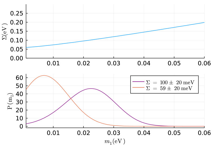
Figure 1: (Top) Correlation between $\Sigma$ and $m_{1}$ assuming the best fit values for the neutrino oscillation angles and mass splittings Zyla et al. (2020). Assuming neutrino masses follow the normal ordering, $\Sigma$ is constrained to be larger than 59 meV. (Bottom) Gaussian probability distributions of $\Sigma$ transformed into probability distributions of $m_{1}$ through a change of variable using the best fit of the neutrino oscillation parameters. The Gaussian distributions $\Sigma=59\pm 20$ meV and $100\pm 20$ meV correspond to the two extreme measurements that DESI and EUCLID can perform.

In our analysis, we combined the likelihoods from the most sensitive $0\nu\beta\beta$-decay experiments which are CUORE Adams et al. (2022), EXO-200 Anton et al. (2019), GERDA Agostini et al. (2020), and KamLAND-Zen Abe et al. (2022). None of these have reported hints for a signal and have set lower limits on its half-life at the level of $10^{25}-10^{26}$ years, corresponding to upper limits on $m_{\beta\beta}$ of the order of 100 meV. We also include the likelihood from the latest analysis of KATRIN Aker et al. (2022) on the electron neutrino mass $m_{\beta}=(c_{12}^{2}\,c_{13}^{2}\,m_{1}^{2}+s_{12}^{2}\,c_{13}^{2}\,m_{2}^{2}+s_{13}^{2}\,m_{3}^{2})^{1/2}$. The parameters of interest for a $0\nu\beta\beta$-decay analysis are collected in the vector $\theta$

$$\theta=(m_{1},\Delta m_{12},\Delta m_{13},s_{12},s_{13},\alpha_{1},\alpha_{2},\mathrm{NME})$$ (3)

The oscillation parameters are incorporated into the analysis using Gaussian terms with central values and uncertainties taken from Ref. Zyla et al. (2020).

By sampling the likelihood function and prior probability distributions, we generate pseudo-data sets for the future $0\nu\beta\beta$-decay experiments and evaluate their average probability to report a discovery, as proposed in Ref. Caldwell and Kroninger (2006). We reproduce the performance of future experiments by using a Poisson counting analysis with fixed background expectation as proposed in Ref. Agostini et al. (2022), from which we also take the input effective background levels and signal efficiencies. We assume ten years of operation for all experiments, corresponding to what the community aims to achieve within the next two decades. The discovery criteria is defined by requiring the posterior odds to be above a certain threshold, i.e.:

$$\mathcal{O}_{1}=\frac{P(D|H_{1})}{P(D|H_{0})}\frac{P(H_{1})}{P(H_{0})}>10,$$ (4)

where $P(D|H)$ are the probabilities of the data given the hypothesis that $0\nu\beta\beta$ decay exists ($H_{1}$) or not ($H_{0}$). $P(H_{1})$ and $P(H_{0})$ are their corresponding priors assumed to be equal. This criteria corresponds to the request that $H_{1}$ is ten times more probable than $H_{0}$ assuming they are initially equally probable. We finally define as discovery probability the fraction of pseudo-datasets satisfying our discovery criteria. Our calculations are performed using the BAT software kit and its native Metropolis-Hastings sampling algorithm Schulz et al. (2020). We determined that the discovery criteria used in this work provides results numerically similar to those of a $3\sigma$ frequentist rejection test of $H_{0}$. More details on our discovery probability calculations are given in the appendix.

We perform our calculations using fixed sets of NME values. We take each set from a specific many-body calculation, and consider calculations Hyvarinen and Suhonen (2015); Šimkovic et al. (2018); Rodriguez and Martinez-Pinedo (2010); López Vaquero et al. (2013); Song et al. (2017); Barea et al. (2015); Deppisch et al. (2020) whose results are available for all isotopes of interest in this analysis, i.e., ⁷⁶Ge, ¹⁰⁰Mo,¹³⁰Te, and ¹³⁶Xe. This choice excludes some NSM and QRPA calculations for which the NME value for ¹⁰⁰Mo is currently not available but it has the advantage that each element in a NME set has correlated systematic uncertainties that partially cancel out when combining data on different isotopes Faessler et al. (2011); Lisi and Marrone (2022). The spread among discovery probabilities computed for different sets of NME values will hence give a rough idea of the uncertainty due to the different many-body methods. However, it will not capture effects coherently affecting all methods, such as the lack of the contact operator Cirigliano et al. (2019) or the so-called “$g_{A}$ quenching” physics Agostini et al. (2022) that we discuss later.

The top panel of Figure 2 shows the $m_{\beta\beta}$ posterior probability distributions computed for a scan of fixed $m_{1}$ values, ranging from $10^{-4}$ to $10^{-2}$ eV. It should not be interpreted as a two-dimensional distribution, but rather as contiguous one-dimensional conditional probability distributions of $m_{\beta\beta}$, each normalized independently. The probability distribution is contained in a well defined part of the parameter space thanks to the accurate measurements available for the neutrino oscillation parameters. The remaining width of $m_{\beta\beta}$ probability distributions is due to the freedom left to the Majorana phases. Our choice of using a uniform prior for these parameters favors the largest $m_{\beta\beta}$ values available at each fixed $m_{1}$ value, including in the region between $10^{-3}-10^{-2}$ eV where specific values of the Majorana phases can lead to vanishing $m_{\beta\beta}$ values. The smaller is the value chosen for $m_{1}$, the smaller is the maximally-allowed value of $m_{\beta\beta}$, whose minimum reaches 0.5 meV for $m_{1}=0$ meV. $0\nu\beta\beta$-decay experiments cut into the upper part of the probability distributions, and are currently ruling out $m_{\beta\beta}$ values above 156 meV Abe et al. (2022), indirectly constraining $m_{1}$ to be $\lesssim 100$ meV. Future experiments will reach discovery sensitivities down to $m_{\beta\beta}$ values of 6 meV depending on the NME values Agostini et al. (2021a).

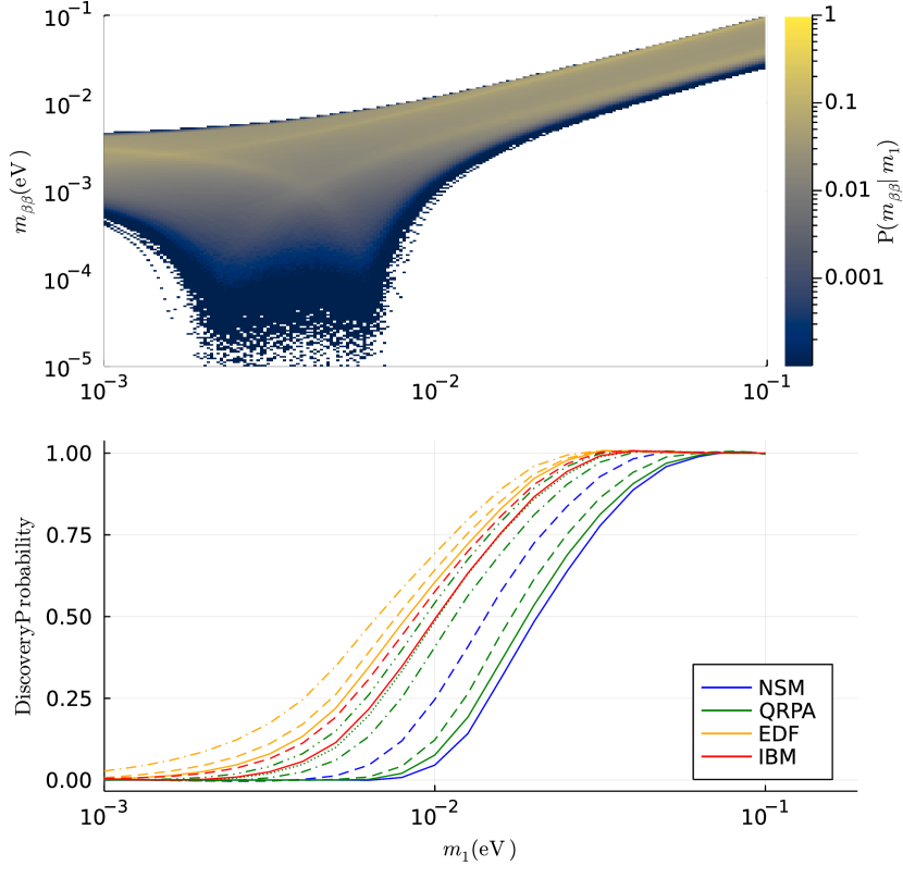
Figure 2: (Top) Conditional one-dimensional posterior probabilities for $m_{\beta\beta}$ computed for a scan of fixed $m_{1}$ values, assuming all available data on neutrinos, normal ordering and a uniform prior on the effective Majorana phases. (Bottom) Discovery probability for a combined analysis of CUPID, LEGEND and nEXO as a function of the true value of $m_{1}$. The probability is computed for different sets of NME values yielding a band for the discovery probability.

The lower panel of Figure 2 shows the combined discovery probability of CUPID, LEGEND and nEXO as a function of $m_{1}$ for all sets of NME values considered. The discovery probability starts at zero when $m_{1}$ is smaller than 1 meV, and continuously grows until it approaches 100% when $m_{1}$ is larger than $\sim$60 meV. The discovery probability varies significantly depending on the considered set of NME values in the $m_{1}$ range 5–50 meV. The larger the NME values, the higher are the discovery probabilities. The discovery probabilities converge below 5 meV and above 50 meV.

Given a theoretical prediction on the value of $m_{1}$, the discovery probabilities in the field of $0\nu\beta\beta$-decay can be directly obtained from the plot in Figure 2. However, we are currently lacking a complete model of fermion masses and theory is not providing strong guidance on the value of $m_{1}$. For this reason, it is relevant to consider scenarios in which $m_{1}$ is a free parameter weakly constrained by indirect information. The drawback of this approach is that, if the information on $m_{1}$ is not strong enough, the results of any analysis are deeply affected by the choice of its prior probability distribution. In particular, any scale-invariant log-flat prior would lead to a non-normalizable posterior distribution unless a cut-off on $m_{1}$ is applied as done in Ref. Caldwell et al. (2017). Other approaches effectively forcing the value of $m_{1}$ to be similar to that of the other two mass eigenvalues have also been explored, see for instance Agostini et al. (2017); Simpson et al. (2017). In the following, we consider a uniform prior distribution on $m_{1}$ from 0 to 600 meV. This prior choice favors $m_{\beta\beta}$ values closer to the parameter space probed by the experiments if one has no other guidance of the parameter range of $m_{1}$. If, however, one includes cosmological bounds on $\Sigma$ the probability distribution for $m_{1}$ is modified and analyses including cosmological data are less affected by the chosen prior on $m_{1}$.

Figure 3 shows the discovery probabilities for CUPID, LEGEND, nEXO and their combination, under four scenarios and for each set of NME values. The first two scenarios show the impact of the use of the current cosmological constraint on $\Sigma$. When considering cosmological models beyond $\Lambda_{\textrm{CDM}}$, much larger neutrino masses are allowed Alvey et al. (2022), and the most stringent information on $m_{1}$ comes from current $0\nu\beta\beta$-decay experiments and from KATRIN. In such a scenario the discovery probabilities are as high as 80% as the uniform prior on $m_{1}$ has significant probability mass at larger $m_{1}$ values. In other words, if one ignores standard cosmological bounds and assumes a flat prior on $m_{1}$, the conclusion is that the discovery of $0\nu\beta\beta$ is quite probable. When the likelihood constraining $\Sigma<120$ meV is included, this penalizes large $m_{1}$ values reducing the discovery probability to values ranging between 20 and 60%.

The speculative scenarios including future measurements of $\Sigma$ show encouraging discovery opportunities. Should $\Sigma$ be right below the current constraints, for instance 100 meV, future $0\nu\beta\beta$-decay experiments are very likely to observe a signal, with discovery probability between 20 and 80%. Even if $\Sigma=59\pm 20$ meV, which is at the bottom of its allowed parameter space, the discovery probabilities are significant, ranging from a few percents to above 40%. The discovery probabilities in these two scenarios are weakly affected by the prior choice on $m_{1}$, for which the measurements on $\Sigma$ gives robust information (see Figure 1). For instance, we estimated that a log-prior on $m_{1}$ with a cutoff as in Caldwell et al. (2017) would reduce these discovery probabilities by a maximum of $30\%$. This indicates that whatever value of $\Sigma$ will be reported by DESI and EUCLID, next-generation $0\nu\beta\beta$-decay experiments will explore a complementary parameter space, where both the measurement of a signal or its exclusion will provide invaluable information.

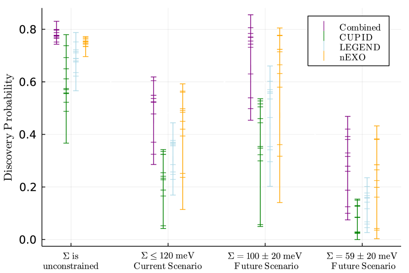
Figure 3: Discovery probabilities for a selection of proposed experiments and their combination under different scenarios and set of NME values. The scenarios differ because of the information included on $\Sigma$, respectively no information, current upper limit, and two possible measurements at the extreme of the currently allowed parameter space. The calculation has been performed using fixed sets of NME values, and each results is shown as an horizontal tick.

The discovery probabilities of the single experiments are similar to each other, and the spread is maximal for nEXO and minimal for LEGEND, consistently with the spread of NME values available for Xe and Mo. When cosmological data are not used, $m_{1}$ is primarily constrained by the current $0\nu\beta\beta$-decay experiments. In this case, increasing the NME values pushes the $m_{\beta\beta}$ probability distribution to lower masses, but also allows future experiments to probe lower $m_{\beta\beta}$ values. The impact of such an interplay becomes negligible in the scenarios in which $\Sigma$ is constrained and the current $0\nu\beta\beta$-decay experiments have a weak impact on the $m_{\beta\beta}$ probability distribution.

The spread of results due to the NME uncertainty remains significant, especially considering that we did not include QRPA calculations for which ¹⁰⁰Mo results are not available. A significant effort is ongoing within the nuclear theory community and will improve the accuracy and precision of NME values. Ab initio calculations have been performed for light and medium-sized nuclei Gysbers et al. (2019), and will soon be available for the heavier isotopes of interest. These new calculations are expected to incorporate more realistic nuclear correlations and corrections to the leading-order operator in chiral effective field theory, e.g. two-body currents, and first results suggest reduced NME values Belley et al. (2021). The inclusion of this so-called “$g_{A}$ quenching” physics can however be at least partially compensated by the previously neglected contact term recently introduced in Ref. Cirigliano et al. (2018), leading to discovery probabilities similar to those shown in Figure 3. Indeed, we have computed that a 20% overall scaling of the NME values for all isotopes (equivalent to a $\sim$10% variation in $g_{a}$) would change the discovery probabilities by 5–10%, not affecting the overall conclusions of our work. The impact of such an overall scaling is marginal as it consistently affects both the current and future experiments.

The combination of all experiments results in an average boost of discovery probabilities of about 20% compared to the mean from single experiments. Additionally, the range of values for the combination is significantly narrowed compared to the set of single experiments, as expected by the partial compensation of NME value fluctuations among the three isotopes.The combination mitigates the least favourable NME values leading to the very small discovery probabilities in single experiments. An other advantage of combining multiple experiments is an increased confidence in a discovery. Indeed, systematic uncertainties related for instance to miss-modelled background components will affect only a single experiment and be mitigated by a combined analysis. Statistical fluctuations will also compensate, providing a lower chance of false discoveries which we estimated to be below the $0.2\%$ level. All these arguments emphasize the value of executing several large-scale $0\nu\beta\beta$ experiments.

In conclusion, precision neutrino cosmology and searches for $0\nu\beta\beta$ decay are heavily entangled and largely complementary. If the neutrino is a Majorana particle in the minimal extension of the Standard Model of particle physics, and the mass ordering is inverted, future $0\nu\beta\beta$-decay experiments will clearly see a signal. The situation for the normal ordering is more complicated, and results from future cosmological experiments will considerably narrow the allowed ranges for $m_{1}$ and therefore the discovery probability of next-generation $0\nu\beta\beta$-decay experiments. If cosmology reports upper bounds on $\Sigma$ also in the future, there is moderate discovery probability for future $0\nu\beta\beta$-decay searches and the question whether the neutrino is a Majorana particle will still be open. However, if cosmological results report a value for the sum of neutrino masses $\Sigma>59$ meV, the chance of discovering $0\nu\beta\beta$-decay will be very significant also for the normal ordering. A non-observation of $0\nu\beta\beta$-decay in this case would give a strong indication that the neutrino is a Dirac particle.

I Acknowledgments

We would like to thank Miguel Escudero Abenza for valuable discussions on cosmology and neutrinos. We are grateful to Giovanni Benato, Kunio Inoue, and Andrea Pocar — as well as to the CUORE, EXO-200, GERDA, and KamLAND-Zen Collaborations — for providing the likelihood functions. M.A. thanks Giovanni Benato, Jason Detwiler, Javier Menéndez and Francesco Vissani for valuable discussions. This work has been supported by the Science and Technology Facilities Council, part of U.K. Research and Innovation (Grant No. ST/T004169/1), the University College London (UCL) Cosmoparticle Initiative, and by the Deutsche Forschungsgemeinschaft (DFG, German Research Foundation) under the Sonderforschungsbereich (Collaborative Research Center) SFB1258 ‘Neutrinos and Dark Matter in Astro- and Particle Physics’.

II Appendix

We present here the calculational procedure for the discovery probability. As a first step, we define two hypotheses:

• $0\nu\beta\beta$ is not present and all counts are background

• $0\nu\beta\beta$ exists and can provide event counts in addition to the background.

The probability of the hypothesis given the data is contained in the posterior probabilities $P(H_{0}|D)$ and $P(H_{1}|D)$. If the probability of $H_{1}$ is larger than $H_{0}$ then a discovery can be claimed. For this purpose, we calculate the posterior odds

$$\mathcal{O}_{1}=\frac{P(H_{1}|D)}{P(H_{0}|D)}.$$ (5)

We define a discovery by $\mathcal{O}_{1}>10$. Assuming that the two hypotheses are exhaustive we can calculate the posterior probabilities with

$$P(H_{i}|D)=\frac{P(D|H_{i})P(H_{i})}{P(D|H_{1})P_{0}(H_{1})+P(D|H_{0})P(H_{0})},$$ (6)

yielding

$$\mathcal{O}_{1}=\frac{P(D|H_{1})}{P(D|H_{0})}\frac{P(H_{1})}{P(H_{0})}.$$ (7)

We set the prior odds $P(H_{1})/P(H_{0})=1$ implying that we take the scenarios to be equally probable. We model the background likelihoods with Poisson distributions

$$P(D|H_{0})=P(\{n\}|H_{0})=\prod_{i}e^{-\lambda_{i}}\frac{\lambda_{i}^{n_{i}}}{n_{i}!},$$ (8)

where the $\lambda_{i}$’s are the background expectation, which is given for each experimental setup individually, $i$ runs over the number of experiments and $\{n\}$ is the collection for the counts reported by the experiments. For hypothesis $H_{1}$, one has to add the signal expectation $\nu_{i}$ which are related to the experimental setups by

$$\nu_{i}=\frac{N_{A}\,ln2}{m_{i}}\,\frac{\mathcal{E}_{i}\,\epsilon_{i}}{T_{1/2}},$$ (9)

with the Avogadro number $N_{A}$, the molar mass of the enriched isotope $m_{i}$, the exposure $\mathcal{E}_{i}$ and the detection efficiency $\epsilon_{i}$ of the experiments, yielding

$$P(\{n\}|\theta,H_{1})=P(\{n\}|\nu(\theta),H_{1})=\prod_{i}e^{-(\lambda_{i}+\nu_{i})}\frac{(\lambda_{i}+\nu_{i})^{n_{i}}}{n_{i}!},$$ (10)

where $\theta$ is the collection of parameters relevant for a $0\nu\beta\beta$ decay discussed in the text. With these definitions we can calculate $P(D|H_{1})$ via

$$P(D|H_{1})=P(\{n\}|H_{1})=\int_{0}^{\infty}P(\{n\}|\nu(\theta))P(\theta|H_{1})d\theta$$ (11)

$$=E(P(\{n\}|\nu(\theta)))_{P(\theta)}.$$ (12)

With the quantities given in equations (8) and (12) we calculate the posterior odds for a given data set. To calculate the discovery probability $P_{D}$, we have to create samples of possible counts the different experiments could report. We also need to sample over the possible parameter values from the analysis of available data. The resulting mathematical expression is

$$P_{D}=E\left[E\left[I\left(\frac{E[P(\{n\}|\theta)]_{P(\theta)}}{P(\{n\}|H_{0})}\right)\right]_{P(\{n\}|\theta)}\right]_{P(\theta)}.$$ (13)

Technically we use $3000$ Markov chain Monte Carlo samples from the posterior probability distribution of the analysis of available data for each investigated scenario (see Figure 3). Then we create $3000$ samples from the investigated experiments for each of these parameter sets. In the last step, we average over the parameter samples again while keeping the specific set of counts fixed. By calculating the posterior odds via (4) for every single created event, we can decide if this specific sample we call a discovery or not and evaluate how many of the investigated samples lead to a discovery. This procedure was followed for the single experiment case already in Caldwell et al. (2017).

References

- Agostini et al. (2022) M. Agostini, G. Benato, J. A. Detwiler, J. Menéndez, and F. Vissani, (2022), arXiv:2202.01787 [hep-ex] .
- Fukugita and Yanagida (1986) M. Fukugita and T. Yanagida, Phys. Lett. B 174, 45 (1986).
- Majorana (1937) E. Majorana, Nuovo Cim. 14, 171 (1937).
- Racah (1937) G. Racah, Nuovo Cim. 14, 322 (1937).
- Schechter and Valle (1982) J. Schechter and J. W. F. Valle, Phys. Rev. D 25, 2951 (1982).
- Minkowski (1977) P. Minkowski, Phys. Lett. B 67, 421 (1977).
- Gell-Mann et al. (1979) M. Gell-Mann, P. Ramond, and R. Slansky, Conf. Proc. C 790927, 315 (1979), 1306.4669 .
- Yanagida (1979) T. Yanagida, Conf. Proc. C 7902131, 95 (1979).
- Mohapatra and Senjanovic (1980) R. N. Mohapatra and G. Senjanovic, Phys. Rev. Lett. 44, 912 (1980).
- Dell’Oro et al. (2016) S. Dell’Oro, S. Marcocci, M. Viel, and F. Vissani, Adv. High Energy Phys. 2016, 2162659 (2016).
- Lattanzi and Gerbino (2018) M. Lattanzi and M. Gerbino, Front. in Phys. 5, 70 (2018).
- Aghanim et al. (2020) N. Aghanim et al. (Planck), Astron. Astrophys. 641, A6 (2020), [Erratum: Astron.Astrophys. 652, C4 (2021)].
- Font-Ribera et al. (2014) Font-Ribera et al., JCAP 05, 023 (2014).
- Ilić et al. (2022) S. Ilić et al. (Euclid), Astron. Astrophys. 657, A91 (2022).
- Zyla et al. (2020) P. A. Zyla et al. (Particle Data Group), PTEP 2020, 083C01 (2020), and 2021 update.
- Esteban et al. (2020) I. Esteban, M. C. Gonzalez-Garcia, M. Maltoni, T. Schwetz, and A. Zhou, JHEP 09, 178 (2020).
- Jimenez et al. (2022) R. Jimenez, C. Pena-Garay, K. Short, F. Simpson, and L. Verde, (2022), arXiv:2203.14247 .
- Gariazzo et al. (2022) S. Gariazzo et al., (2022), arXiv:2205.02195 .
- Agostini et al. (2021a) M. Agostini, G. Benato, J. A. Detwiler, J. Menéndez, and F. Vissani, Phys. Rev. C 104, L042501 (2021a).
- Feruglio et al. (2002) F. Feruglio, A. Strumia, and F. Vissani, Nucl. Phys. B 637, 345 (2002), [Addendum: Nucl. Phys. B 659, 359–362 (2003)].
- Benato (2015) G. Benato, Eur. Phys. J. C 75, 563 (2015).
- Armstrong et al. (2019) W. R. Armstrong et al. (CUPID), (2019), arXiv:1907.09376 .
- Abgrall et al. (2021) N. Abgrall et al. (LEGEND), (2021), arXiv:2107.11462 .
- Kharusi et al. (2018) S. A. Kharusi et al. (nEXO), (2018), arXiv:1805.11142 .
- Lisi and Marrone (2022) E. Lisi and A. Marrone, Phys. Rev. D 106, 013009 (2022), arXiv:2204.09569 .
- Gráf et al. (2022) L. Gráf, M. Lindner, and O. Scholer, (2022), arXiv:2204.10845 .
- Agostini et al. (2017) M. Agostini, G. Benato, and J. Detwiler, Phys. Rev. D 96, 053001 (2017).
- Caldwell et al. (2017) A. Caldwell, M. Ettengruber, A. Merle, O. Schulz, and M. Totzauer, Phys. Rev. D 96, 073001 (2017).
- Dell’Oro et al. (2019) S. Dell’Oro, S. Marcocci, and F. Vissani, Phys. Rev. D 100, 073003 (2019).
- Agostini et al. (2021b) M. Agostini, G. Benato, S. Dell’Oro, S. Pirro, and F. Vissani, Phys. Rev. D 103, 033008 (2021b).
- Adams et al. (2022) D. Q. Adams et al. (CUORE), Nature 604, 53 (2022).
- Anton et al. (2019) G. Anton et al. (EXO-200), Phys. Rev. Lett. 123, 161802 (2019), arXiv:1906.02723 .
- Agostini et al. (2020) M. Agostini et al. (GERDA), Phys. Rev. Lett. 125, 252502 (2020).
- Abe et al. (2022) S. Abe et al. (KamLAND-Zen), (2022), arXiv:2203.02139 .
- Aker et al. (2022) M. Aker et al. (KATRIN), Nature Phys. 18, 160 (2022).
- Caldwell and Kroninger (2006) A. Caldwell and K. Kroninger, Phys. Rev. D 74, 092003 (2006).
- Schulz et al. (2020) O. Schulz et al., (2020), arXiv:2008.03132 .
- Hyvarinen and Suhonen (2015) J. Hyvarinen and J. Suhonen, Phys. Rev. C 91, 024613 (2015).
- Šimkovic et al. (2018) F. Šimkovic, A. Smetana, and P. Vogel, Phys. Rev. C 98, 064325 (2018).
- Rodriguez and Martinez-Pinedo (2010) T. R. Rodriguez and G. Martinez-Pinedo, Phys. Rev. Lett. 105, 252503 (2010).
- López Vaquero et al. (2013) N. López Vaquero, T. R. Rodríguez, and J. L. Egido, Phys. Rev. Lett. 111, 142501 (2013).
- Song et al. (2017) L. S. Song, J. M. Yao, P. Ring, and J. Meng, Phys. Rev. C 95, 024305 (2017).
- Barea et al. (2015) J. Barea, J. Kotila, and F. Iachello, Phys. Rev. C 91, 034304 (2015).
- Deppisch et al. (2020) F. F. Deppisch, L. Graf, F. Iachello, and J. Kotila, Phys. Rev. D 102, 095016 (2020).
- Faessler et al. (2011) A. Faessler, G. L. Fogli, E. Lisi, A. M. Rotunno, and F. Simkovic, Phys. Rev. D 83, 113015 (2011), arXiv:1103.2504 .
- Cirigliano et al. (2019) Cirigliano et al., Phys. Rev. C 100, 055504 (2019).
- Simpson et al. (2017) F. Simpson, R. Jimenez, C. Pena-Garay, and L. Verde, JCAP 06, 029 (2017).
- Alvey et al. (2022) J. Alvey, M. Escudero, N. Sabti, and T. Schwetz, Phys. Rev. D 105, 063501 (2022), arXiv:2111.14870 [hep-ph] .
- Gysbers et al. (2019) P. Gysbers et al., Nature Phys. 15, 428 (2019).
- Belley et al. (2021) A. Belley, C. G. Payne, S. R. Stroberg, T. Miyagi, and J. D. Holt, Phys. Rev. Lett. 126, 042502 (2021).
- Cirigliano et al. (2018) V. Cirigliano et al., Phys. Rev. Lett. 120, 202001 (2018).