definition

How a Small Amount of Data Sharing Benefits Distributed Optimization and Learning

Mingxi Zhu Scheller College of Business, Georgia Institute of Technology, Atlanta, GA 30332 mingxiz@stanford.edu

Yinyu Ye Management Science & Engineering, Stanford University, Stanford, CA 94305, yyye@stanford.edu

Distributed optimization algorithms have been widely used in machine learning. While those algorithms have the merits in parallel processing and protecting data security, they often suffer from slow convergence. This paper focuses on how a small amount of data sharing could benefit distributed optimization and learning. Specifically, we examine higher-order optimization algorithms including distributed multi-block alternating direction method of multipliers (ADMM) and preconditioned conjugate gradient method (PCG). The contribution of this paper is three-folded. First, in theory, we answer when and why distributed optimization algorithms are slow by identifying the worst data structure. Surprisingly, while PCG algorithm converges slowly under heterogeneous data structure, for distributed ADMM, data homogeneity leads to the worst performance. This result challenges the common belief that data heterogeneity hurts convergence, highlighting the need for a universal approach on altering data structure for different algorithms. Second, in practice, we propose a meta-algorithm of data sharing, with its tailored applications in multi-block ADMM and PCG methods. By only sharing a small amount of prefixed data (e.g. $1\%$), our algorithms provide good quality estimators in different machine learning tasks within much fewer iterations, while purely distributed optimization algorithms may take hundreds more times of iterations to converge. Finally, in philosophy, we argue that even minimal collaboration can have huge synergy, which is a concept that extends beyond the realm of optimization analysis. We hope that the discovery resulting from this paper would encourage even a small amount of data sharing among different regions to combat difficult global learning problems.

Distributed Learning; Distributed Optimization; Data Sharing

1 Introduction

Distributed optimization algorithms have been widely used in large scale machine learning problems [Eckstein and Bertsekas (1992a), Boyd et al. (2011), Nishihara et al. (2015)]. The benefit of distributed algorithms is two-folded. Firstly, by distributing the workload to local data centers, distributed optimization algorithms could potentially reduce the required computation time from parallel computing and processing. A salient feature of most machine learning problems is that the objectives are separable, and distributed optimization algorithms could exploit the benefit of having separable objectives. Secondly, distributed optimization algorithms are preferred when data communication between agents is costly. However, in practice, distributed optimization algorithms often suffer from slow convergence to the target tolerance level when applied to large scale machine learning problems [Ghadimi et al. (2014), Nilsson et al. (2018)].

This work aims at providing a solution to boost the convergence speed for applying distributed optimization algorithms in machine learning problems, from both theoretical and practical aspects. We first provide a theoretical answer to the following questions: why distributed optimization algorithms can sometimes have unsatisfactory performance in terms of convergence speed, and what kind of data distribution leads to such slow convergence. Surprisingly, we found that, contradicting to the well-established results that data heterogeneity hurts convergence speed, for certain algorithms, data homogeneity leads to worst convergence speed. This result sheds light on the importance for the need of a universal approach on altering data distribution across agents for different distributed optimization algorithms. With theoretical guidance, this paper provides a meta data-sharing algorithm that only requires sharing a small amount of pre-fixed data to build a global data pool. And we numerically show that only a small amount of data share is sufficient to improve the convergence speed for different distributed optimization algorithms. With tailored design on utilizing the shared data to different distributed algorithms, we are able to enjoy both the benefit from faster convergence from data sharing, and from parallel computing by keeping the main structure of the optimization algorithms closer to a distributed manner. Sharing a small amount of data is also of great practical importance, as most of the time, sharing all the data from local agents and building a centralized optimization algorithm may not be a feasible solution due to either high cost of data communication, or constraints on communication regarding privacy and security concerns. However, building a global data pool from a one-time communication on a small amount of pre-fixed data is way less costly compared to centralized optimization by sharing all data to central server. Besides, when the local agents process a hybrid of private data and synthetic data, sharing synthetic data across agents is feasible and would not violate privacy or security constraints [Giuffrè and Shung (2023)].

More importantly, philosophically, the results provided in this paper confirm the synergy of even minimal degree of collaboration, which is a concept that goes beyond the regime of optimization analysis. Many studies have examined the benefit of data sharing, in aspects of data-driven decision making, supply chain management and revenue management to name a few [Lee et al. (2000), Shang et al. (2016), Feasey and de Streel (2020), Choe et al. (2023)]. In this work, we show that data sharing not only increases the social surplus and individual utility, but also improves the efficiency in optimization algorithms. And such benefit could be achieved with even $5\%$ of sharing pre-fixed data. And the synergy of collaboration across agents is amplified in data-driven decision making, through both the knowledge spillover effect in utility analysis, and the improved efficiency when applying optimization algorithms in data-driven problems. Hence, we hope that the discovery resulted from this paper would encourage even a small amount of data sharing among different regions to combat difficult global learning problems.

2 Literature Review

Our paper examines how a small amount of data sharing benefits distributed optimization algorithms when applying to machine learning problems, with focus on multi-block ADMM algorithm and PCG methods. In this section, we first review literature related to multi-block ADMM and PCG algorithms. One stream of work, federated learning, is also closely related to applying distributed optimization in machine learning. We review the literature in federated learning and point out the differences between our work and federated learning, in hope that the results presented in this paper would also shed lights in federated learning algorithm design. Lastly, we then review literature related in distributed optimization and federated learning, with focus on the negative impacts of data heterogeneity. Contrary to those study, our result shows that data heterogeneity can sometimes benefit higher-order optimization algorithms, which suggests that a simple solution to mitigate the challenge of data heterogeneity is to “order-up”.

ADMM algorithms have been widely viewed as an optimization method that lies in between first order methods and second order methods, and many researchers have found that ADMM algorithms are well-suited for large scale statistical inference and machine learning problems [Boyd et al. (2011), Mohan et al. (2014), Huang and Sidiropoulos (2016), Taylor et al. (2016)]. The traditional two-block ADMM algorithm and its convergence analysis have been excessively explored [Gabay and Mercier (1976), Eckstein and Bertsekas (1992a), He et al. (2012), Monteiro and Svaiter (2013), Glowinski (2014), Deng and Yin (2016)]. However, the two-block ADMM is not well-suited for solving large scale machine learning problems, as it requires processing and factorization for a large matrix, which is both time and space consuming [Stellato et al. (2018), Zarepisheh et al. (2018), Lin et al. (2017)]. Instead, variants of multi-block ADMM emerges, several prevailing multi-block ADMM algorithms include distributed ADMM [Eckstein and Bertsekas (1992b), He and Yuan (2012), Ouyang et al. (2013)], cyclic ADMM [Hestenes (1969), Powell (1978)], and randomized multi-block ADMM [Sun et al. (2020), Mihić et al. (2020)]. While distributed ADMM is known to be robust for convergence under any choice of step size parameter, many studies have also found that the convergence rate of primal distributed ADMM is highly sensitive to the choice of step size, and may suffer from slow convergence once the step-size is not well-tuned [Ghadimi et al. (2014), Nishihara et al. (2015), Iutzeler et al. (2015)]. On the other hand, while cyclic ADMM can boost up the convergence rate sometimes compared with distributed ADMM, it is not guaranteed to converge for all instances in theory [Chen et al. (2017)]. Mihić et al. (2020) first introduced data-share across different blocks in multi-block ADMM algorithm. However, their algorithm requires a full randomized data exchange across blocks at each iteration, which may not be feasible in practice if there is data security concerns. Moreover, it might require more computation and communication cost under full randomization scheme.

Similar as ADMM algorithms, conjugate gradient methods have also been considered as lying between first order gradient methods and second order Newton’s method [Luenberger et al. (1984), Shewchuk et al. (1994)]. Conjugate gradient methods have been recently applied to not only solving large scale linear system, but also machine learning tasks with parallel implementation [Le et al. (2011), Helfenstein and Koko (2012), Hsia et al. (2018)]. The convergence of conjugate gradient method has been well-studied, and many studies assure on the point that preconditioning is indispensable to algorithm performance improvement, as ill-conditioning of matrix often leads to divergence, which leads to the prevailing preconditioned conjugate gradient method (PCG) [Axelsson and Lindskog (1986), Kaasschieter (1988), Kaporin (1994), Herzog and Sachs (2010)]. Recently, Drineas and Mahoney (2016) introduce a randomized sampling process to improve the computational efficiency in preconditioning of large-scale matrix. However, their algorithm is designed to solve large scale linear algebra problems, and cannot be directly applied to distributed learning problems.

Federated learning is also related to our work. Federated learning is a machine learning technique that trains the data/observations in decentralized local data sets [Konečnỳ et al. (2015), Bonawitz et al. (2019)]. In the setup of federated learning, most literature assumes that the center only has access to the intermediate training weights of local agents without exchanging raw data [McMahan et al. (2017), Stich (2018), Khaled et al. (2020), Yuan and Ma (2020)]. And the common prevailing algorithms employed in federated learning are first-order based (e.g. FedAvg, FSVRG [Mangasarian (1995), McMahan et al. (2017), Zhou and Cong (2017), Nilsson et al. (2018)]), while several studies “order-up” the gradient based algorithsm [Agafonov et al. (2022)]. Although the regime of our study in distributed optimization with data sharing does not directly belong to the setup in federated learning, where the raw data remains private. We still believe that in practice, when local agents possess a hybrid of data sets which contains both privacy-sensitive and less privacy-sensitive data, exchanging a small amount of less privacy-sensitive raw data across agents could benefit algorithm performance. And we hope our results in distributed optimization could shed lights in federated learning algorithm design.

In all previous streams of literature related to distributed optimization and federated learning, data heterogeneity across local agents typically leads to adverse effects. Specifically, for first-order algorithms, data heterogeneity is often viewed as a major challenge in speeding up training methods [Wang et al. (2020), Woodworth et al. (2020), Karimireddy et al. (2020)]. Several survey papers [Gao et al. (2022), Ye et al. (2023)] have also summarized the negative impact of data heterogeneity in federated learning framework. And currently, many first-order based distributed learning algorithms provide unsatisfying training results with heterogeneous data sources [Li et al. (2022), Mendieta et al. (2022)]. In our paper, we show that contrary to those results, when applying higher-order optimization algorithms, data heterogeneity may have positive impacts on boosting up the convergence speed. This suggests that one way to mitigate the challenge of data heterogeneity may simply be order-up the optimization algorithms, and shift from first-order based training methods to higher order optimization methods in machine learning.

Our main theoretical contribution to the previous literature in multi-block ADMM, PCG methods, and impact of data heterogeneity to distributed optimization, is on discovering when and why the distributed optimization algorithms suffer from slow convergence. To answer those questions, we apply new technical method with matrix Jensen inequality to show that for multi-block distributed ADMM, data homogeneity hurts convergence. The high level intuition lies in that the ADMM algorithm updates the dual variable by averaging over the local auxiliaries/estimators which are essentially the product of inverse of local matrices. And the dual updating has the least momentum when the local matrices are similar by matrix Jensen inequality. Hence, any data sharing that increases the difference between local matrices would boost up the momentum for dual updating. While our proof techniques depend on the linear mapping of the algorithm which is only valid when the objective is quadratic under least square regression, in the numerical experiments, we found that data-sharing also helps logistic regression. As whether multi-block ADMM would still have linear convergence rate for general objectives is still an open problem (Han et al. (2018),Liu et al. (2018)), we decide to focus on the regime of direct comparing the linear convergence rate under quadratic objectives in this paper, and put the analysis with general convex objectives in future works. Numerically, we contribute to previous streams of literature by presenting a novel idea of creating a data pool with a small amount of prefixed shared data across local agents, and utilizing this data pool in each iteration later. We find that such approach is effective for both least square and logistic machine learning tasks.

This paper is organized as follows. Section 3 answers when and why multi-block ADMM and PCG methods suffer from slow convergence. We show that while data heterogeneity hurts PCG methods, it benefits multi-block ADMM methods under certain regime. Section 4 provides the design of a meta-algorithm of data sharing, with tailored application to multi-block ADMM and PCG methods. We further apply the tailored algorithms to least square and logistic regressions with both synthetic and public benchmark data sets (UCI machine learning regression repository [Dua and Graff (2017)]). Numerically, we show that with $5\%$ of data share, our algorithms converge ten or hundreds more times faster than those without data sharing. Section 5 concludes our work, provides future research directions, and echos on encouraging even small amount of data sharing among different regions to combat difficult global learning problems.

3 Theory

In this paper, we mainly focus on multi-block distributed Alternating Direction Method of Multipliers (ADMM) and preconditioned conjugate gradient methods (PCG), which are both known as the algorithms in between the first order gradient descent method and the second order Newton’s methods. Specifically, we consider the following distributed statistical learning problem. Let $(\BFx_{j}\in\operatorname{\mathbb{R}}^{1\times p},y_{j}\in\operatorname{\mathbb{R}})$ be the model data and dependent variable pair. The data pair $(\BFx_{j},y_{j})$ locates at different local agents. We assume there are $b$ agents, each of the agent possesses $s_{i}$ numbers of observations $(\BFX_{i}=[\BFx_{1};\dots;\BFx_{s_{i}}]\in\operatorname{\mathbb{R}}^{s_{i}\times p},\ \BFy_{i}=[y_{1};\dots;y_{s_{i}}]\in\operatorname{\mathbb{R}}^{s_{i}\times 1})$, with $i\in\{1,\dots,b\}$, with $(\BFx_{i,j},y_{i,j})$ being the $j^{th}$ data pair associated with $i^{th}$ agent. Let the total number of observations $n=\sum^{b}_{i=1}s_{i}$. We denote $\BFX=[\BFX_{1};\dots;\BFX_{b}]\in\operatorname{\mathbb{R}}^{n\times p}$, and $\BFy=[\BFy_{1};\dots\BFy_{b}]$ as the aggregate model data matrix and dependent variable vector. In this paper, we consider the case where centralized optimizing by uploading all local data to one machine is not feasible, which implies that one cannot directly operates with $(\BFX,\BFy)$. This is common in practice when either the data communication across agents is costly, or there is privacy/security constraints associated with certain data sets.

A decision maker tries to find $\BFbeta\in\operatorname{\mathbb{R}}^{p}$ that minimizes the following global loss function

$$F((\BFX,\BFy);\BFbeta)=\sum^{b}_{i=1}\sum^{s_{i}}_{j=1}f((\BFx_{i,j},y_{i,j});\BFbeta)$$ (1)

where $f((\BFx,y);\BFbeta)$ is the regression model choice of the decision maker. Several commonly used regression models include least squares regression $f((\BFx,y);\BFbeta)=\|\BFx\BFbeta-y\|^{2}_{2}$, ridge $f((\BFx,y);\BFbeta)=\|\BFx\BFbeta-y\|^{2}_{2}+\alpha\|\BFbeta\|^{2}_{2}$, lasso $f((\BFx,y);\BFbeta)=\|\BFx\BFbeta-y\|^{2}_{2}+\alpha\|\BFbeta\|_{1}$, elastic net $f((\BFx,y)=\|\BFx\BFbeta-y\|^{2}_{2}+\alpha\|\BFbeta\|_{1}+(1-\alpha)\|\BFbeta\|^{2}_{2}$, and logistic regression $f((\BFx,y);\BFbeta)=log(1+\exp(-y\BFx\BFbeta))$.

3.1 Application in distributed multi-block distributed ADMM method

Consider the following classic formulation to solve problem (1) with distributed ADMM by introducing auxiliary $\BFbeta_{i}$ to the optimization problem for each local agent.

$$\min \quad\sum^{b}_{i=1}\ \sum^{s_{i}}_{j=1}f((\BFx_{i,j},y_{i,j});\BFbeta_{i})$$ (2)

$$s.t. \quad\BFbeta_{i}-\BFbeta=0\quad\forall\ i=1,\dots,b$$

To apply the primal distributed ADMM algorithm, the decision maker solves the relaxed augmented Lagrangian problem. Let $\BFlambda_{i}$ be the dual with respect to the constraint $\BFbeta_{i}-\BFbeta=0$, and $\rho_{p}$ the step size to the primal distributed ADMM. The augmented Lagrangian is thus given by

$${L(\BFbeta_{i},\BFbeta,\BFlambda_{i})=\sum^{b}_{i=1}\ \sum^{s_{i}}_{j=1}f((\BFx_{i,j},y_{i,j});\BFbeta_{i})+\sum^{b}_{i=1}\BFlambda_{j}^{T}(\BFbeta_{i}-\BFbeta)+\sum^{b}_{i=1}\frac{\rho_{p}}{2}(\BFbeta_{i}-\BFbeta)^{T}(\BFbeta_{i}-\BFbeta)}$$ (3)

The algorithm of primal distributed ADMM is as follows.

Initialization: $t=0$, step size $\rho_{p}\in\operatorname{\mathbb{R}}^{+}$ $\BFbeta_{t}\in\operatorname{\mathbb{R}}^{p}$, $\BFlambda_{t,i}\in\operatorname{\mathbb{R}}^{p}$, $\BFbeta_{t,i}\in\operatorname{\mathbb{R}}^{p}$ for all $i\in\{1,\dots,b\}$, and stopping rule $\tau$ 

while $t\leq\tau$ do

     Each local agent $i$ updates $\BFbeta_{t+1,i}$in parallel by  

     $\BFbeta_{t+1,i}=\argmin_{\BFbeta_{i}\in\operatorname{\mathbb{R}}^{p}}\ \sum^{s_{i}}_{j=1}f((\BFx_{i,j},y_{i,j});\BFbeta_{i})+\BFlambda_{t,i}^{T}(\BFbeta_{i}-\BFbeta^{t})+\frac{\rho_{p}}{2}(\BFbeta_{i}-\BFbeta_{t})^{T}(\BFbeta_{i}-\BFbeta_{t})$ 

     Decision maker updates  

     $\BFbeta_{t+1}=\frac{1}{b}\sum^{b}_{i=1}\BFbeta_{t+1,i}+\frac{1}{b\rho_{p}}\sum^{b}_{i=1}\BFlambda_{t,i}$, $\BFlambda_{t+1,i}=\BFlambda_{t,i}+\rho_{p}(\BFbeta_{t+1,i}-\BFbeta_{t+1})$  

end while

Output: $\BFbeta_{\tau}$ as global estimator

Algorithm 1 Primal Distributed ADMM for solving (2)

Specifically, when applying to least square regression, the problem becomes a quadratic optimization with linear constraints. In this section, we focus on providing the theory for the least square regression.

$$\min_{\BFbeta_{i},\BFbeta} \quad\sum^{b}_{i=1}\frac{1}{2}(\BFX_{i}\BFbeta_{i}-\BFy_{i})^{T}(\BFX_{i}\BFbeta_{i}-\BFy_{i})$$ (4)

$$s.t. \quad\BFbeta_{i}-\BFbeta=0\qquad\forall\ i$$

While many studies have already studied the impact of global matrix conditioning [Eckstein and Bertsekas (1992b), Iutzeler et al. (2015), Makhdoumi and Ozdaglar (2017)], our work is the first to study how local data structure impacts the convergence speed for distributed ADMM. In order to focus on the impact of local data structure, we first introduce the following assumption on the global data matrix $\BFX$. We assume the global covariance matrix $\BFX^{T}\BFX$ has fixed conditioning number. Without loss of generality, we further assume that the global covariance matrix is normalized by its Frobenius norm, hence the largest eigenvalue of the global covariance matrix is smaller than $1$ . Fixing the global matrix conditioning allows us to purely focus on the effect on how data structure influences convergence. Also it’s worth noticing that any data share across local centers would not influence the conditioning of the global covariance matrix. However, data sharing still significantly changes the local data structure, hence, influencing the convergence speed.

Assumption 3.1

The regressor matrix $\BFX$ is normalized by its Frobenius norm $\|\BFX\|_{F}$, and the smallest and largest eigenvalue of $\BFX^{T}\BFX$, $\underline{q}$ and $\bar{q}$ are fixed, with $\BFX^{T}_{i}\BFX_{i}\succ 0$ for all $i\in\{1,\dots,b\}$.

Before introducing the main theorem, we provides an illustrating example on showing how data structure influences the convergence rate under the case matrix conditioning $\underline{q}$ and $\bar{q}$ fixed. Consider a simple case with feature dimensionality $p=1$, number of agents $b=2$ and step size $\rho_{p}=1$. In the first scenario, the original model matrix $\tilde{\BFX}_{i}$ and the model matrix after normalizing by Frobenius norm, $\BFX_{i}$ are given by

$${\tilde{\BFX}_{1}=\begin{bmatrix}0.99\\ 0.01\end{bmatrix},\quad\tilde{\BFX}_{2}=\begin{bmatrix}0.9\\ 0.1\end{bmatrix},\quad{\BFX}_{1}=\begin{bmatrix}0.7379\\ 0.0075\end{bmatrix},\quad{\BFX}_{2}=\begin{bmatrix}0.6708\\ 0.0745\end{bmatrix}}$$ (5)

Here, as feature dimensionality $p=1$, $\bar{q}=\underline{q}=1$. If we directly applying Algorithm 1, the linear convergence rate, which is also the spectrum of the linear mapping matrix, is given by $0.6661$. However, consider the second scenario, where we just swap the distribution of data without changing model matrix condition $\underline{q}$ and $\bar{q}$.

$${\tilde{\BFX}_{1}=\begin{bmatrix}0.99\\ 0.9\end{bmatrix},\quad\tilde{\BFX}_{2}=\begin{bmatrix}0.01\\ 0.1\end{bmatrix},\quad{\BFX}_{1}=\begin{bmatrix}0.7379\\ 0.6708\end{bmatrix},\quad{\BFX}_{2}=\begin{bmatrix}0.0075\\ 0.0745\end{bmatrix}}$$ (6)

The convergence rate of applying Algorithm 1 is given by $0.5264$. In fact, one could show that, for primal distributed ADMM the worst case convergence rate is $0.6667$ and the best convergence rate one could achieve is $0.5$ with $b=2$ and feature dimensionality $p=1$. Here, data structure significantly influences on the convergence rate of primal distributed ADMM from near worst convergence rate to near optimal convergence rate. From this illustrating example, we notice that if different agent shares similar model covariance matrix $\BFD_{i}=\BFX_{i}^{T}\BFX_{i}$, primal distributed ADMM suffers from convergence.

We further generalize the previous example. Let $\BFD_{i}=\BFX_{i}^{T}\BFX_{i}$, and $\BFc_{i}=-\BFX_{i}^{T}\BFy_{i}$, following algorithm 1, the updating process becomes

$$(\rho_{p}\BFI+\BFD_{i})\BFbeta^{t+1}_{i}= \rho_{p}\BFbeta^{t}-\BFlambda^{t}_{i}-\BFc_{i}$$ (7)

$$\BFbeta^{t+1}= \frac{1}{b}\sum_{i}\BFbeta^{t+1}_{i}+\frac{1}{b\rho_{p}}\sum_{i}\BFlambda^{t}_{i}$$

$$\BFlambda^{t+1}_{i}= \BFlambda^{t}_{i}+\rho_{p}(\BFbeta^{t+1}_{i}-\BFbeta^{t+1})$$

The process in (7) could be represented as a linear mapping system. Following Iutzeler et al. (2015), ${\BFxi^{k+1}=\rho_{p}\bar{\BFbeta}^{k+1}+\bar{\BFlambda}^{k}}$ is sufficient to represent the system dynamics, where $\bar{\BFbeta}^{k+1}=[\BFbeta^{k+1}_{1};\dots;\BFbeta^{k+1}_{i};\dots;\BFbeta^{k+1}_{b}]\in\operatorname{\mathbb{R}}^{bp\times 1}$, and $\bar{\BFlambda}^{k}=[\BFlambda^{k}_{1};\dots;\BFlambda^{k}_{i};\dots;\BFlambda^{k}_{b}]\in\operatorname{\mathbb{R}}^{bp\times 1}$. The mapping matrix of the primal distributed ADMM is given by

$${\BFM_{p}=\left(\BFI-\BFP-\left(\BFI+\frac{\BFD}{\rho_{p}}\right)^{-1}\right)(\BFI-2\BFP)}$$ (8)

where ${\BFP=b^{-1}1_{b}1_{b}^{T}\otimes\BFI_{p}}$ is the projection matrix. Here $1_{b}$ is size $b\times 1$ all one vector; $\BFI_{p}$ is size $p\times p$ identity matrix; ${\BFD=diag([\BFD_{1},\dots,\BFD_{i},\dots,\BFD_{b}])}$ is the block diagonal matrix of $\BFD_{i}$; and $\otimes$ represents the tensor product of $b^{-1}1_{b}1_{b}^{T}$ and $\BFI_{p}$.

As shown before, for least square regression the primal distributed ADMM uses $\BFM_{p}$ for linear updating. Since we are comparing algorithms under linear convergence regime, we define the convergence rate of primal distributed ADMM as the spectral radius of linear mapping matrix $\BFM_{p}$, $\rho(\BFM_{p})$. From previous literature, primal distributed ADMM converges for any constant step size and $\rho(\BFM_{p})<1$ (Eckstein and Bertsekas (1992b)). The data structure that leads to worst convergence rate depends on the choice of step size $\rho_{p}$. In the following theorem, we provides the results when step size is relatively large.

Theorem 3.2

For $\rho_{p}>\bar{q}$, the linear convergence rate of distributed ADMM is upper bounded by $\frac{b\rho_{p}}{b\rho_{p}+\underline{q}}$, and the upper bound is achieved when $\BFX^{T}_{i}\BFX_{i}=\BFX^{T}_{j}\BFX_{j}$ for all $i,j\in\{1,\dots,b\}$.

Theorem 3.2 provides the tight upper bound on the convergence rate of distributed ADMM. To our knowledge, this is the first result on providing how data structure influences the convergence rate, and provides tight upper bound on the convergence rate of primal distributed ADMM with fixed model matrix conditioning $\bar{q}$ and $\underline{q}$. Surprisingly, data homogeneity leads to worst data structure for higher order optimization algorithms, which challenges the conventional belief on data heterogeneity hurts convergence for distributed learning algorithms. The detailed proof is provided in appendix A.1. We present the sketch of proof here for high level intuition. To show that such convergence rate attains upper bound, we first show that the eigenvalue of $\BFM_{p}$ is real, which is not trivial as $\BFM_{p}$ is non-symmetric. With this, one could further apply matrix Jensen equality to prove Theorem 3.2. The key proof lies in the intrinsic updating rules of distributed ADMM that involves taking average of local auxiliary variables when updating the global variable $\BFbeta$ and the dual variables $\BFlambda_{i}$. And updating each local auxiliary variable is based on taking the inverse of the local covariance matrix. When $\BFX^{T}_{i}\BFX_{i}$ and $\BFX^{T}_{j}\BFX_{j}$ are closer, averaging the inverse of local covariance matrices provides smaller momentum on pushing the dual variables to converge to the KKT point.

The following corollary shows the benefit of data sharing under data homogeneity.

Corollary 3.2.1

When $\BFX^{T}_{i}\BFX_{i}=\BFX^{T}_{j}\BFX_{j}$ for all $i,j\in\{1,\dots,b\}$, any data share that changes the local covariance matrix strictly improves the linear convergence rate of distributed ADMM.

It’s worth to have some further discussions on Theorem 3.2. Firstly, notice that the upper bound on convergence speed is increasing with respect to number of data centers $b$, and decreasing with $\underline{q}$. These two effects are more intuitively direct, as more number of centers hurts convergence, and ill conditioning of model matrix also hurts convergence. More importantly, from Theorem 3.2 we know data homogeneity hurts convergence for higher order optimization algorithms as distributed ADMM. However, one popular technique in machine learning is data augmentation, where the decision maker creates synthetic agents by augmenting existing data through scaling, flipping, or rotation, to name a few. Such data augmentation technique tends to increase data homogeneity across agents. While data homogeneity may benefits the first order algorithms [Wang et al. (2020), Li et al. (2022)], it hurts higher order distributed primal-dual optimization algorithms. And one needs to carefully apply data augmentation together with higher order optimization algorithms.

Theorem 3.2 provides bounds on convergence rate and worst case data structure when step size is relatively large. We introduce the following theorem when step size is relatively small and $b=2$. Let $\underline{\lambda}(\BFD_{i})$ be the smallest eigenvalue of $\BFD_{i}$, and $q_{1}$ be the smallest eigenvalue among all $\BFD_{i}$. From Assumption 3.1, $q_{1}>0$. The following theorem on worst case data structure and upper bound on convergence rate holds for $b=2$.

Theorem 3.3

For $\rho_{p}<q_{1}$ and $b=2$, the convergence rate of distributed ADMM is upper bounded by $\frac{\bar{q}}{2\rho_{p}+\bar{q}}$, and the upper bound is achieved when $\BFX^{T}_{1}\BFX_{1}=\BFX^{T}_{2}\BFX_{2}$.

Theorem 3.3 provides the worst case data structure when $b=2$. The detailed proof is provided in appendix A.2. The worst case data structure is similar as in Theorem 3.2. When $b=2$, data homogeneity still hurts convergence. However, for $b>2$, with relative small step size $\rho_{p}<q_{1}$, the system becomes more complex. Firstly, the data structure with $\BFD_{i}=\BFD_{j}$ for all $i,j\in\{1,\dots,b\}$ does not provide an upper bound for the convergence rate. In appendix, we show that under the structure where $\BFD_{i}=\BFD_{j}$ for all $i,j\in\{1,\dots,b\}$ and $\rho_{p}<q_{1}$, the convergence rate is given by $\frac{\bar{q}}{b\rho_{p}+\bar{q}}$, which decreases as number of blocks increases. This suggests that the data structure of $\BFD_{i}=\BFD_{j}$ may not be the worst case data structure when $b>2$. In the following proposition, we provide an upper bound on the convergence rate for smaller step size $\rho_{p}$ and $b>2$.

Proposition 3.4

For $\rho_{p}<q_{1}$, the convergence rate of distributed ADMM is upper bounded by $\frac{\bar{q}}{\rho_{p}+\bar{q}}$, and there exists a data structure that provides convergence rate of $\frac{\bar{q}-(b-2)\rho_{p}}{2\rho_{p}+\bar{q}-(b-2)\rho_{p}}$.

The proving technique used in Proposition 3.4 is different from Theorem 3.2. Instead, we use the classic bound on $\rho(M)\leq\rho(\frac{1}{2}M^{T}+\frac{1}{2}M)$ for non-symmetric matrix. Hence, the bound is not tight. The data structure that provides convergence rate of $\frac{\bar{q}-(b-2)\rho_{p}}{2\rho_{p}+\bar{q}-(b-2)\rho_{p}}$ tries to mimic the worst case data structure under two block distributed ADMM by having two agents possessing the majority of data with similar structures, and the rest of agents possessing minimum data to ensure that local covariance matrices have strictly positive eigenvalues. And the convergence rate of the data structure provided in Proposition 3.4 is strictly higher compared with the data structure of $\BFD_{i}=\BFD_{j}$ for all $i,j\in\{1,\dots,b\}$.

Lastly, we compare our results with other common optimization method that is also widely used in learning across local data centers, first-order method of gradient descent. Here, we assume the decision maker could perform a synchronized aggregation scheme with local full gradient information, which differs from the prevailing federated learning algorithms. Nevertheless, updating with synchronized full gradients provides an upper bound for federated learning algorithms, where federated learning uses sampled gradient with asynchronous updating. While distributed ADMM converges for any constant step size, gradient descent method converges only when step size is within some specific range. For least square regression, the convergence rate is given by the spectrum of matrix $M_{GD}=(\BFI-\rho_{p}\BFX^{T}\BFX)$, where $\rho_{p}$ is the step size. We provide the following corollary on comparing the convergence rate between gradient descent and distributed ADMM for least square regression under same choice of step size. From proposition 3.5, the convergence rate of gradient descent method is better than the convergence rate of distributed ADMM for only a specific sweet range of step size.

Proposition 3.5

For $\rho_{p}\in(0,s_{1})\cup(s_{2},\infty)$, $\rho(M_{p})<\rho(M_{GD})$, where

$$s_{1}=\min\left(\frac{1}{\underline{q}}-\bar{q},q_{1}\right),\quad s_{2}=\frac{2b-\bar{q}\underline{q}+\sqrt{4b^{2}+(\bar{q}\underline{q})^{2}}}{2b\bar{q}}$$

From proposition 3.5, firstly, we are convinced that higher order optimization algorithms like distributed ADMM have its merits in faster and robust convergence. As gradient descent method is not guaranteed to converge for any choice of step size. Secondly, it’s not surprising that choosing a good step size is crucial for faster convergence, for all algorithms. However, our result shows that distributed ADMM method outperforms gradient method for a large range of step size choices. This implies the first order method is more sensitive to the parameter selection, and the first order method could only perform well within a small range of “sweet-spot” step size.

3.2 Application in PCG method

In this section, we consider using PCG method for solving problem (4), which is equivalent as solving the following linear system with distributed conjugate gradient method.

$${\sum^{b}_{i=1}\BFX^{T}_{i}\BFX_{i}=\sum^{b}_{i=1}\BFX^{T}_{i}\BFy_{i}}$$ (9)

The algorithm of conjugate gradient method with distributed preconditioners is as follows.

Initialization: $t=0$, $\BFbeta_{0}$ $\BFr^{i}_{0}=\BFX^{T}_{i}\BFy$; $\BFbeta_{0}$; local pre-conditioner matrices $\BFH_{i}$, $\BFp^{i}_{0}=\BFH_{i}\BFr^{i}_{0}$ stopping rule $\tau$ 

Decision maker receives $\BFr^{i}_{0}$, $\BFp^{i}_{0}$, calculates $\BFr_{0}=\sum_{i}\BFr^{i}_{0}$, $\BFp_{0}=\sum_{i}\BFp^{i}_{0}$ and broadcasts it to each agent 

while $t\leq\tau$ do

     Each agent calculates $\BFr^{T}_{k}\BFH_{i}\BFr_{k}$ and $\BFp^{T}_{k}\BFX^{T}_{i}\BFX_{i}\BFp_{k}$ and sends to decision maker 

     Decision maker updates $\alpha_{k}=\frac{\sum_{i}\BFr^{T}_{k}\BFH_{i}\BFr_{k}}{\sum_{i}\BFp^{T}_{k}\BFX^{T}_{i}\BFX_{i}\BFp_{k}}$ and sends to each agent 

     Each agent calculates $\alpha_{k}\BFX^{T}_{i}\BFX_{i}\BFp_{k}$ and sends to decision maker 

     Decision maker updates $\BFbeta_{k+1}=\BFbeta_{k}+\alpha_{k}\BFp_{k}$, $\BFr_{k+1}=\BFr_{k}-\sum_{i}\alpha_{k}\BFX^{T}_{i}\BFX_{i}\BFp_{k}$ and sends to each agent 

     Each agent calculates $\BFH_{i}\BFr_{k+1}$, $\BFr^{T}_{k+1}\BFH_{i}\BFr_{k+1}$ and sends to decision maker 

     Decision maker updates $t_{k}=\frac{\sum_{i}\BFr^{T}_{k+1}\BFH_{i}\BFr_{k+1}}{\sum_{i}\BFr^{T}_{k}\BFH_{i}\BFr_{k}}$, $\BFp_{k+1}=\sum_{i}\BFH_{i}\BFr_{k+1}+t_{k}\BFp_{k}$ and sends to each agent

end while

Output: $\BFbeta_{\tau}$ as global estimator

Algorithm 2 Conjugate gradient method with local preconditioning

From the algorithm description, conjugate gradient with local preconditioning takes more communications between agents and the decision maker compared with distributed ADMM algorithm, which may not be ideal, if the cost of communication between agents and decision maker is high. In the meantime, local preconditioning performs good if the sum of the local preconditioning matrix $\BFH=\sum_{i}\BFH_{i}$ is a good approximation of $(\BFX^{T}\BFX)^{-1}$, where $\BFX^{T}\BFX=\sum_{i}\BFX_{i}^{T}\BFX_{i}$. However, without data sharing, each of the agent could only determine $\BFH_{i}$ based on local information of $\BFX_{i}^{T}\BFX_{i}$, and without data sharing, approximating $\BFX^{T}\BFX$ with only local information is hard. However, if one can share sampled data that is representative to the local agent’s data distribution, the local preconditioning with data sharing could perform much better.

We first introduce an approach on constructing local pre-conditioners with shared data, and provide a theoretical improvement on convergence rate for preconditioned conjugate gradient (PCG) with data sharing. We further show that preconditioning is helpful for faster convergence with numerical experiments. Let $\BFX_{\sigma_{i}}\in\operatorname{\mathbb{R}}^{r_{i}\times p}$ be the selected shared data from agent $i$ with $\BFX_{i}\in\operatorname{\mathbb{R}}^{s\times p}$. We construct local preconditioning matrix with global data share as $\BFH^{g}_{i}=(\frac{1}{b}\BFX_{i}^{T}\BFX_{i}+\sum_{j\neq i}\frac{s}{r_{i}}\BFX^{T}_{\sigma_{i}}\BFX_{\sigma_{i}})^{-1}$. Intuitively, $\BFH_{i}$ tries to create an estimate of $(\BFX^{T}\BFX)^{-1}$ with the information from the sampled data. We compare the convergence rate of local preconditioning with shared data to conjugate gradient without preconditioning, and conjugate gradient with local preconditioning of $\BFH_{i}=(\BFX_{i}^{T}\BFX_{i})^{-1}$. The following example shows that data sharing is essential for preconditioning.

Proposition 3.6

When solving the linear system $\BFA\BFx=\BFb$, where $\BFA=\sum^{b}_{i=1}\BFA_{i}$, there exists data structure such that the condition number of $\BFH\BFA$ could be arbitrarily large if we construct local preconditioning matrix $\BFH$ without data share; while with data share, the condition number of $\BFH\BFA$ decreases and converges to $1$.

Consider the case where we have two agents, both of them possess $s$ observations with feature dimension $p=2$. Agent $1$ possess $(\BFX_{1},\BFy_{1})$, and $\BFX_{1}=[\BFx^{1}_{1};\dots;\BFx^{1}_{i};\dots;\BFx^{1}_{s}]$ with $\BFx^{1}_{i}=\frac{1}{\sqrt{s}}(1,\xi_{i})$. Agent $2$ possess $(\BFX_{2},\BFy_{2})$, and $\BFX_{2}=[\BFx^{2}_{1};\dots;\BFx^{2}_{j};\dots;\BFx^{2}_{b}]$ with $\BFx^{2}_{j}=\frac{1}{\sqrt{s}}(1,\xi_{j})$. $\xi_{i}$ and $\xi_{j}$ are i.i.d. Gaussian random variables $\epsilon_{1}N(0,1)$ and $\epsilon_{2}N(0,1)$. In order to perform least square regression, one needs to solve the linear system of $\sum^{b}_{i=1}\BFA_{i}=\BFb$, where

$${\BFA_{1}=\BFX^{T}_{1}\BFX_{1}=\begin{bmatrix}1&a_{1}\\ a_{1}&b_{1}\end{bmatrix}\quad\BFA_{2}=\BFX^{T}_{1}\BFX_{1}=\begin{bmatrix}1&a_{2}\\ a_{2}&b_{2}\end{bmatrix}\quad\BFb=\sum^{b}_{i=1}\BFX^{T}_{i}\BFy_{i}}$$ (10)

with $a_{1}$ $a_{2}$ following gaussian distribution $\frac{\epsilon_{1}}{b}N(0,1)$, $\frac{\epsilon_{2}}{b}N(0,1)$ respectively, and $b_{1}$, $b_{2}$ following chi-squared distribution $\frac{\epsilon_{1}^{2}}{b^{2}}\chi_{b}$ and $\frac{\epsilon_{2}^{2}}{b^{2}}\chi_{b}$ respectively. As the number of observations $s$ increases, $\BFA_{1}$ and $\BFA_{2}$ converges to

$${\BFA_{1}=\begin{bmatrix}1&0\\ 0&\epsilon_{1}^{2}\end{bmatrix}\quad\BFA_{2}=\begin{bmatrix}1&0\\ 0&\epsilon_{2}^{2}\end{bmatrix}}$$ (11)

Let $\epsilon_{2}=\frac{1}{\epsilon_{1}}$, and take $\epsilon_{1}$ to be small enough, without data sharing, the local preconditioning matrix at agent $1$ is given by $\BFH_{1}=(\BFX_{1}^{T}\BFX_{1})^{-1}$, and the conditioning number of $\BFH_{1}\BFA$ is $\frac{\epsilon^{2}+1}{2\epsilon^{2}}$. The local preconditioning matrix at agent $2$ is given by $\BFH_{2}=(\BFX_{2}^{T}\BFX_{2})^{-1}$, and the conditioning number of $\BFH_{2}\BFA$ is $\frac{2}{1+\epsilon^{2}}$. Simply apply local preconditioning provides the aggregated preconditioning matrix of $\BFH_{local}=\BFH_{1}+\BFH_{2}$, and the conditioning number of $\BFH_{local}\BFA$ is $\frac{(\epsilon^{2}+1)^{2}}{4\epsilon^{2}}$. However, with any linear fraction amount of data share, if we construct local preconditioning matrix with global data share as $\BFH^{g}_{i}=(\frac{1}{b}\BFX_{i}^{T}\BFX_{i}+\sum_{j\neq i}\frac{s}{r_{i}}\BFX^{T}_{\sigma_{i}}\BFX_{\sigma_{i}})^{-1}$, with $\BFH_{global}=\sum^{b}_{i=1}\BFH^{g}_{i}$, one could show that as $s$ increases, the conditioning number of $\BFH_{global}\BFA$ converges to $1$. In the numerical results, we assume local agents have heterogeneous data sources. We implement PCG method with local preconditioners and global preconditioners with data sharing, and we compared the result with conjugate gradient method without preconditioning. Under PCG method, data heterogeneity hurts convergence. However, a small amount of data sharing helps providing a much better preconditioner, which mitigates the challenge of data heterogeneity.

To summarize the theory section, we find that data heterogeneity has complex effect on algorithm convergence rate. While under PCG method, data heterogeneity hurts convergence, under multi-block distributed ADMM method, data heterogeneity benefits convergence. This result highlights the need for a universal approach on altering data distribution for different algorithms. In the following section, we introduce a meta data-sharing algorithm, and provide numerical evidence on how data sharing could significantly improve convergence speed for different higher order algorithms.

4 Algorithms Design and Numerical Results

4.1 Data sharing algorithm

In this section, we describe the sampling procedure to enable data sharing across local agents. The meta-algorithm of data sharing is simple and easy to implement – it samples $\frac{\alpha}{b}\%$ of data uniform randomly from each agents, and builds a global data pool with the total $\alpha\%$ prefixed sampled data. The benefit of having a global data pool is two-folded – (a) it allows the decision maker to have the freedom on changing the local data structure; (b) it allows the decision maker to have a unbiased sketch of the global higher order information of the objective function, e.g., the sketch of Hessian information.

Sampling Procedure : Randomly sample $\frac{\alpha}{b}\%$ of data pairs from each agent one-time 

Let $\BFr\in\operatorname{\mathbb{Z}}^{m\times 1}$ be the index of selected data ($m=\left\lfloor{\alpha\%n}\right\rfloor$). Let $\BFr_{i}$ be the index of selected data at agent $i$, and $\BFl_{i}$ be the index of data remains local at agent $i$ 

Output: global data pool $(\BFX_{\BFr},\BFy_{\BFr})=([\BFX_{{\BFr}_{1}};\dots;\BFX_{{\BFr}_{b}}],[\BFy_{{\BFr}_{1}};\dots;\BFy_{{\BFr}_{b}}])$ with shared access to all local agents  

Algorithm 3 Meta-algorithm of data sharing

With the meta-algorithm of data sharing and the global data pool, now the distributed optimization algorithms have the access to a sketch of the global data. From numerical evidence, we are convinced that we only need a small amount of data share to improve the convergence speed. Setting $\alpha$ at a low level also allows us to enjoy the benefits from distributed optimization with parallel computation. As the majority of data still remains at local, the algorithm could take advantages from such structure. For example, the algorithm could pre-factorize the local data observation matrix for faster computation. Hence, without specification, we fix $\alpha$ to be $5\%$ across numerical experiments. After we decide on the desirable level of data share , for each distributed optimization algorithm, we still need to carefully design how the algorithm should utilize the global data pool efficiently with theory guidance. In the next section, we implement the algorithms with careful and tailored design on utilizing data sharing for multi-block ADMM and PCG method.

The numerical result section is organized as follows. Section 4.2 provides the algorithm design for multi-block ADMM with data-sharing. We further show the numerical results for both the least square regression and the logistic regression, and compare our performance with distributed multi-block ADMM without data sharing, together with other variants of multi-block ADMM algorithms. Section 4.3 provides the algorithm design for PCG method with data sharing .

4.2 Apply data sharing in multi-block ADMM methods

In this section, we present results on both the least square regression and logistic regression. For least square regression, we test the algorithms on the benchmark of UCI machine learning repository regression data (Dua and Graff (2017)). And we compare the absolute loss among different algorithms, with absolute loss ${AL=\|\BFbeta^{*}-\hat{\BFbeta}\|_{2}}$, where $\BFbeta^{*}$ is the optimal estimator and $\hat{\BFbeta}$ is the estimator produced by each algorithm. We further add a L2 regularization for all regression problems in order to guarantee the uniqueness of $\BFbeta^{*}$. For logistic regression, we generate the synthetic data with Gaussian noise and the ground truth estimator $\BFbeta^{*}$. We further compare the absolute loss ${AL=\|\BFbeta^{*}-\hat{\BFbeta}\|_{2}}$, where $\BFbeta^{*}$ is the optimal estimator and $\hat{\BFbeta}$ is the estimator produced by each algorithm.

Firstly, from previous result, we know that the worst case data structure for distributed ADMM depends on the relations between the step size and the local data matrix conditioning. And making the local data structure differ from each other would improve the convergence speed. Hence, a simple and direct way to improve the performance of distributed ADMM is to allocate all the global data pool to one existing agent/block, in order to make that block have different data structure from others. We test the modified distributed ADMM with global data, and compare it with classic distributed ADMM in UCI machine learning repository regression data. With fixed number of iteration equals to $200$, block number equals to $4$, and percentage of sample $\alpha=5\%$, the accuracy of estimator $\beta$ improves for 13 out of 14 problem instances. Besides,compared with the distributed ADMM without data sharing, in average distributed ADMM with data sharing decreases the the absolute loss by $20\%$.

However, $20\%$ decrease in absolute loss is not satisfying. Here, we carefully design a randomized multi-block ADMM algorithm to better utilize the global data pool. We further introduce a tailored multi-block ADMM algorithm – the Dual Randomly Assembled and Permuted ADMM (DRAP-ADMM). We use the least square regression as an example to illustrate the idea of DRAP-ADMM. One could design DRAP-ADMM for different loss functions by introducing the conjugate functions.

Introducing the auxiliary $\zeta$, the primal problem could also be formulated as

$$\min_{\BFzeta} \quad\frac{1}{2}\BFzeta^{T}\BFzeta$$ (12)

$$s.t. \quad\BFX\BFbeta-\BFy=\BFzeta$$

And let $\BFt$ be the dual variables with respect to the primal constraints ${\BFX\BFbeta-\BFy=\BFzeta}$. Taking the dual with respect to problem (12), we have

$$\min_{\BFt} \quad\frac{1}{2}\BFt^{T}\BFt+\BFy^{T}\BFt$$ (13)

$$s.t. \quad\BFX^{T}\BFt=0$$

The augmented Lagrangian is thus given by

$${L(\BFt,\BFbeta)=\frac{1}{2}\BFt^{T}\BFt+\BFy^{T}\BFt-\BFbeta^{T}\BFX^{t}+\frac{\rho_{d}}{2}\BFt^{T}\BFX\BFX^{t}\BFt}$$ (14)

The global estimator $\BFbeta$ is the dual variable with respect to the constraint $\BFX^{T}\BFt=0$ and $\rho_{d}$ be the step-size of dual problem. The reason we take dual is that, the dual variables $\BFt$ serves as a label for each (potentially) exchanged data pair, and the randomization is more effective in the dual space. We show that simply taking the dual does not improve the convergence speed. The following proposition guarantees that, the primal distributed algorithm and dual distributed algorithm are exactly the same in terms of computation and convergence rate. The proof is provided in appendix A.5.

Proposition 4.1

The primal distributed ADMM algorithm and the dual distributed ADMM algorithm have exactly the same linear convergence rate if the step size for primal and dual algorithms satisfies $\rho_{p}\rho_{d}=1$ when applied to the least square regression under the partition of blocks with $\BFX=[\BFX_{1};\dots;\BFX_{b}]$ and $\BFy=[\BFy_{1};\dots;\BFy_{b}]$.

Proposition 4.1 states that by only taking the dual of the problem would not impact the convergence speed, and more delicate design on the algorithms is required to enjoy the benefit of data sharing. Hence, we design the Dual Randomly Assembled and Permuted ADMM (DRAP-ADMM) under the inspiration of Mihić et al. (2020). DRAP-ADMM updates the auxiliary variables following a random permuted order across each agent. We present the high level idea on how we utilize the global data pool as follows. Firstly, the meta-algorithm of data sharing randomly selects a subset of data $(\BFX_{\BFr_{i}},\BFy_{\BFr_{i}})$ from agent $i$, and builds the global data pool $(\BFX_{r},\BFy_{r})$. When designing the algorithm, each agent $i$ may first pre-compute and pre-factorize $\BFX_{\BFl_{i}}^{T}\BFX_{\BFl_{i}}^{T}$ in order to enjoy the benefit of the distributed structure, where $\BFX_{\BFl_{i}}$ is the local data at agent $i$. Then, at each iteration, each agent $i$ receives a random sample (without replacement) from the global data pool. The size of received data from global data pool is the same as the size that the agent $i$ contributes to the pool initially. Finally, we random permute the update order across agents at each iteration. The general algorithm of DRAP-ADMM is provided in Algorithm 4.

Initialization: $t=0$, global data pool $(\BFX_{r},\BFy_{r})$, step size $\rho_{d}\in\operatorname{\mathbb{R}}^{+}$ $\BFt_{t}\in\operatorname{\mathbb{R}}^{n}$, $\BFbeta_{t}\in\operatorname{\mathbb{R}}^{p}$, and stopping rule $\tau$ 

while $t\leq\tau$ do

     Random permute $\BFr$ to $\sigma_{t}(\BFr)$, partition $\sigma_{t}(\BFr)=[\sigma^{1}_{t}(\BFr);\dots;\sigma^{b}_{t}(\BFr)]$ according to $|r_{i}|$ (size of $\BFr_{i}$) 

     Random permute the block-wise update order $\xi_{t}(b)=[\xi^{1}_{t},\dots,\xi^{b}_{t}]$ 

     For $i=\xi^{1}_{t},\dots,\xi^{b}_{t}$ 

     Let $\BFsigma^{i}_{t}=\BFl_{i}\cup\sigma^{i}_{t}(\BFr)$. Agent $i$ updates $\BFt^{\BFsigma^{t}_{i}}_{t+1}=\arg\min_{BFt\in\operatorname{\mathbb{R}}^{|B_{i}|}}\ L(\BFt^{\BFsigma^{t}_{1}}_{t+1},\dots,\BFt^{\BFsigma^{t}_{i-1}}_{t+1},\BFt,\BFt^{\BFsigma^{t}_{i+1}}_{t},\dots,\BFt^{\BFsigma^{t}_{b}}_{t},\BFbeta^{t})$ 

     Decision maker updates $\BFbeta_{t+1}=\BFbeta_{t}-\rho_{d}\BFX^{T}\BFt_{t+1}$ 

end while

Output: $\BFbeta_{\tau}$ as global estimator

Algorithm 4 DRAP-ADMM

As the majority of data still remains local, DRAP-ADMM could both enjoy the benefit of pre-factorization for solving local training tasks, and utilize the shared data to change the local data structure constantly, in order to avoid an unfavorable data structure that leads to slow convergence. In order to better utilize the global data pool, we use random permuted updating order instead of distributed updating order. In appendix A.6, we show the benefit of having a random permute updating – it improves the convergence rate under the worst case data structure compared with distributed updating scheme. Further, a random assemble of local blocks with global data pool would further help improve the convergence speed, and following a similar proof in Sun et al. (2015) and Mihić et al. (2020), one could show that DRAP-ADMM converges in expectation for linearly constrained quadratic optimization problems.

There are several other variants of multi-block ADMM algorithms, including the symmetric Gauss-Seidel multi-block ADMM (double-sweep ADMM) [Floudas and Pardalos (2008),Xiao et al. (2019)] and the random-permuted ADMM [Sun et al. (2020)]. In the following numerical experiments provided in Table 1, we use UCI machine learning regression data Dua and Graff (2017) to first compare the performance of DRAP-ADMM with (1) primal distributed ADMM, (2) double-sweep ADMM, (3) cyclic-ADMM and (4) RP-ADMM. Besides, since the meta-algorithm of data sharing could also be applied to primal-distributed ADMM, double-sweep ADMM, and RP-ADMM in a similar way as in DRAP-ADMM, we also compare the DRAP-ADMM with (5) primal distributed ADMM with data-share, (6) double-sweep ADMM with data-share, and (7) RP-ADMM with data-share. We fix step-size to be $\rho=1$ for both the primal algorithms and the dual algorithms in order to eliminate the effect of step-size choices. And we set the percentage of shared data $\alpha=5\%$. The data set has dimensionality of $n=463,715$ and $p=90$. From this set of experiments, we are convinced that, firstly, the performance of multi-block ADMM algorithm significantly improves with only a small amount of data share. Secondly, the random permute updating order seems to be the most compatible algorithm to a small amount of data-sharing, compared with other multi-block updating orders.

	Fix run time $=100$ s	Fix number of iteration $=200$
Primal Distributed ADMM	$2.98\times 10^{-3}$	$4.10\times 10^{-2}$
Double-Sweep ADMM	$5.92\times 10^{-3}$	$3.44\times 10^{1}$
Cyclic ADMM	$5.66\times 10^{-6}$	$3.44\times 10^{1}$
Random Permuted ADMM	$6.62\times 10^{-6}$	$3.44\times 10^{1}$
Primal Distributed ADMM with data sharing	$2.41\times 10^{-3}$	$4.01\times 10^{-2}$
Double-Sweep ADMM with data sharing	$3.80\times 10^{-9}$	$1.44\times 10^{-5}$
Cyclic ADMM with data sharing	$3.07\times 10^{-9}$	$1.13\times 10^{-5}$
DRAP-ADMM	$1.12\times 10^{-9}$	$9.25\times 10^{-6}$

Table 1: Absolute Loss of different multi-block ADMM algorithms for L2 regression estimation on data set Year Prediction MSD

From previous experiments, we are convinced that DRAP-ADMM performs better than the other variants of multi-block ADMM methods. In the following numerical results, we compare DRAP-ADMM with primal distributed ADMM without data sharing. Firstly, we examine the sensitivity of convergence speed to percentage of data shared. We find that, $\alpha$ does not need to be very large for significant efficiency improvement, and a small amount of data sharing is sufficient to boost convergence speed. The following figure (Figure LABEL:fig:1) reports the sensitivity of convergence speed to the percentage of data shared. We fix the same convergence criteria to be $\|\BFbeta_{t}-\BFbeta_{t-1}\|\leq 10^{-4}$ for all different values of $\alpha$. It’s worth mentioning that the required time for convergence with no data shared ($\alpha=0$) is 2403.72 seconds. And in Figure LABEL:fig:1 (a), by sharing even $1\%$ of data, the required time to converge decreases to 221.60 seconds. Similarly, the required number of iterations for converging to the same target tolerance level with no data shared is 3952. And in Figure LABEL:fig:1 (b), by sharing $1\%$ of data, the required number of iterations to converge decreases to 307.

As we only need a small amount of data sharing, in the following experiments, we fix $\alpha\%=5\%$. The following table shows more numerical results we performed on UCI machine learning repository. We set number of agents to be $4$. We fix the step-size $\rho_{p}=\rho_{d}=1$ for primal distributed ADMM and DRAP-ADMM. Note setting step-size equals to $1$ does not favor the primal ADMM nor the dual ADMM, as we show that the primal distributed ADMM and dual distributed ADMM share the same convergence rate when $\rho_{p}\rho_{d}=1$. We consider two stopping rules, fixing the same number or iteration, or the same run time.

	Fix run time = 100 s		Fix number of iteration = 200
	Primal distributed	DRAP-ADMM	Primal distributed	DRAP-ADMM
Bias Correction	$1.60\times 10^{-3}$	$3.71\times 10^{-10}$	$3.20\times 10^{-3}$	$6.31\times 10^{-7}$
Bike Sharing Beijing	$8.43\times 10^{-4}$	$9.57\times 10^{-12}$	$2.03\times 10^{-2}$	$6.61\times 10^{-6}$
Bike Sharing Seoul	$2.60\times 10^{-3}$	$1.71\times 10^{-8}$	$8.87\times 10^{0}$	$5.80\times 10^{-3}$
Wine Quality Red	$3.45\times 10^{-15}$	$2.31\times 10^{-14}$	$8.10\times 10^{-3}$	$1.22\times 10^{-7}$
Wine Quality White	$7.36\times 10^{-15}$	$1.24\times 10^{-13}$	$2.40\times 10^{-3}$	$1.56\times 10^{-6}$
Appliance Energy	$5.02\times 10^{-12}$	$1.61\times 10^{-9}$	$7.56\times 10^{-1}$	$4.77\times 10^{-5}$
Online News Popularity *	$9.42\times 10^{-16}$	$3.23\times 10^{-15}$	$7.70\times 10^{-4}$	$4.63\times 10^{-8}$
Portugal 2019 Election *	$3.97\times 10^{-16}$	$4.97\times 10^{-14}$	$3.22\times 10^{-5}$	$1.99\times 10^{-10}$
Relative Location of CT	$1.65\times 10^{-13}$	$6.44\times 10^{-12}$	$1.29\times 10^{0}$	$4.79\times 10^{-4}$
SEGMM GPU	$2.63\times 10^{-13}$	$2.20\times 10^{-13}$	$4.60\times 10^{-3}$	$2.65\times 10^{-6}$
Superconductivity Data	$1.25\times 10^{-1}$	$2.98\times 10^{-6}$	$6.97\times 10^{-1}$	$4.99\times 10^{-4}$
UJIIndoorLoc Data	$3.76\times 10^{-1}$	$4.48\times 10^{-8}$	$8.45\times 10^{-1}$	$2.53\times 10^{-2}$
Wave Energy Converters	$3.40\times 10^{-3}$	$7.12\times 10^{-10}$	$7.70\times 10^{-3}$	$2.39\times 10^{-7}$
Year Prediction MSD	$3.60\times 10^{-3}$	$4.56\times 10^{-9}$	$3.91\times 10^{-2}$	$2.64\times 10^{-5}$

* The covariance matrix’s spectrum is of $10^{20}$, we scale each entry by $\sqrt{n}$.

Table 2: Absolute Loss on L2 regression estimation

From Table 2, we observe that compared with primal distributed ADMM, a small amount of data sharing with DRAP-ADMM algorithm could attain a good quality predictor within much fewer number of iterations or time. Specifically, with 200 iterations, DRAP-ADMM significantly outperforms primal distributed ADMM. This suggests that DRAP-ADMM algorithms with a small amount of data sharing could be a good solution when the cost per iterations is high. For example, in practice, when conducting regression prediction with healthcare trial data, the decision maker (researcher) would have to present physically to each hospitals in order to perform optimization with local data. Hence, minimizing number of iteration required would be a major objective for decision maker when performing estimation across agents. Nonetheless, we observe that DRAP-ADMM still enjoys some benefit even when we fix the run time.

For general regression analysis including logistic regression, DRAP-ADMM would still apply. The logistic regression minimizes the following objective

$${\min\sum^{b}_{i=1}\sum^{s_{i}}_{j=1}log(1+\exp(-y_{i,j}\BFx_{i,j}\BFbeta))}$$ (15)

with $y_{i,j}\in\{-1,1\}$. Similarly one could apply distributed ADMM to solve logistic regression following Algorithm 1. One need to take the conjugate function of the primal objective, and solves a different optimization problem for each agent. When designing the ADMM method for logistic regression, one could introduce the auxiliary variables in order to further improve the efficiency of the algorithm. For DRAP-ADMM, let $\mathcal{X}=\BFy\cdot\BFX$, we solve the following dual problem

$$\min \quad\sum^{b}_{i=1}\sum^{s_{i}}_{j=1}t_{i,j}log(t_{i,j})+(1-t_{i,j})log(1-t_{i,j})$$ (16)

$$s.t. \quad\mathcal{X}^{T}\BFz\ =\ 0\quad\cdots\BFbeta$$

$$\quad\BFt-\BFz\ =\ 0\quad\cdots\BFxi$$

In Table 3, we present the result on comparing the performances across gradient descent method (with backtracking step-size), primal distributed ADMM and DRAP-ADMM (with step-size equals to 1). A widely used algorithm for solving logistic problem is via Newton’s method. To further compare the algorithms, we select the benchmark algorithm to be the Newton’s method. We need to point out here that the classic Newton’s method requires centralized learning and optimization, which is not the focus of this paper. Nonetheless, we use centralized Newton’s method as the benchmark, and show that distributed optimization with data sharing could outperform centralized optimization method in aspect of convergence rate. Similarly, we fix $\alpha=5\%$. We report the relative ratio in the absolute loss with benchmark of centralized Newton’s method. The relative ratio in the absolute loss is defined as $r_{AL}=\frac{AL_{\textup{ALG}}-AL_{\textup{newton}}}{AL_{\textup{newton}}}$. We fix block numbers equals to $4$ and the number of iterations to be $10$ for all the different algorithms. We expect the Newton’s method to perform well and a positive relative ratio of $r_{AL}$ is not surprising, as we allow the Newton’s method to perform centralized optimization. However, notice that $r_{AL}<0$ implies that under fixed iteration, the algorithm outperforms centralized Newton’s method with smaller absolute value. We report the average of relative ratio in the absolute loss for each size of problem instances with $20$ sample of experiments.

	Gradient Descent	Primal Distributed	DRAP-ADMM
$n=500,\ p=20$	$8.18\times 10^{-3}$	$9.55\times 10^{-3}$	$-6.73\times 10^{-3}$
$n=800,\ p=40$	$2.53\times 10^{-3}$	$2.97\times 10^{-3}$	$-5.89\times 10^{-3}$
$n=1000,\ p=100$	$4.38\times 10^{-4}$	$5.18\times 10^{-4}$	$-2.23\times 10^{-3}$

Table 3: Relative ratio of absolute loss on logistic regression

From Table 3, we observe that primal distributed ADMM method performs similarly as gradient method. Several previous studies have already shown that ADMM method may not be suitable for logistic regression (e.g. Gopal and Yang (2013)). However, it’s worth mentioning that with $5\%$ of data sharing, multi-block ADMM could even out-perform centralized optimization method in terms of convergence speed. These results shed light on the importance of data sharing in the design of multi-block ADMM method. With a small amount of data sharing, one could hugely boost the convergence speed for multi-block ADMM method.

4.3 Apply data sharing in PCG methods

In this section, we apply data sharing algorithm in PCG method. We use the global data pool to construct more efficient local preconditioning matrices. With global data pool $\BFX^{g}$, we could construct the local preconditioning matrix

$${\BFH_{i}=\frac{1}{b}[\BFX^{T}_{i}\BFX_{i}+\sum_{j\neq i}\frac{s_{j}}{|\BFr_{j}|}\BFX_{\BFr_{j}}^{T}\BFX_{\BFr_{j}}]^{-1}}$$ (17)

Intuitively, we use the sampled data to sketch the data structure from other agents in order to estimate the global Hessian. The following numerical experiment considers the synthetic data with 2 agents. Each agent has number of observations $n=1000$ with feature dimension $p=500$. Data possessed in agent $1$ follow independent and identical standard Gaussian distributed. Data possessed in agent $2$ follow independent and identical uniform distribution. We report the relative residuals in L2 norm, $\|\BFb-\BFA\BFx_{t}\|_{2}/\|\BFb\|_{2}$, at each iteration $t$. From Figure (2), we are convinced that the preconditioning with global data pool performs better than all the preconditioning methods without data share.

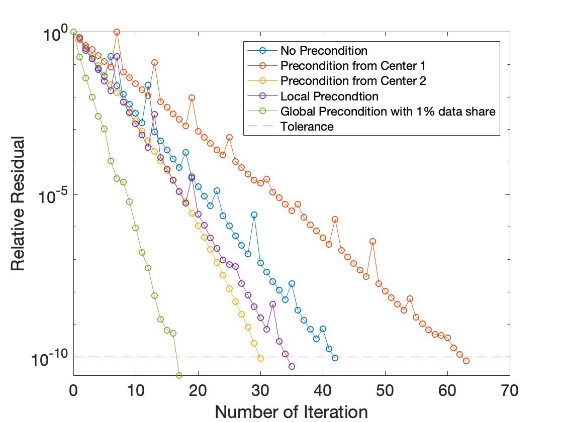
Figure 2: Performance of PCG method

5 Conclusions

In this paper, we focus on how a small amount of data sharing benefits distributed optimization and learning, with focus on higher order optimization algorithms including distributed multi-blcok alternating direction method of multipliers (ADMM) method and preconditioned conjugate gradient (PCG) method. Theoretically, we answer the questions on when and why distributed optimization algorithms may sometimes suffer from slow convergence. Surprisingly, while PCG method suffers under data heterogeneity, for distributed ADMM algorithm, data heterogeneity may lead to faster convergence, which is contrary to conventional result that data heterogeneity hurts convergence. To answer the question of why this counter-intuitive phenomenon happens in distributed ADMM, we show that the key lies in the mechanism for updating dual variables by averaging across local estimators. And data homogeneity leads to weakening the momentum for dual updating. This result not only suggests that a simple approach to mitigate the challenge of data heterogeneity is to “order-up” the optimization algorithms, but also highlights the need for a universal approach, which is easy to implement in practice, on altering the local data structures to boost convergence rate for different optimization algorithms. With the guidance from theory works, we further develop a meta-algorithm of data sharing that builds a global data pool from pulling a small amount of prefixed data from each agent. We observe that sharing a small amount of data across agents may have huge synergy in improving algorithm convergence speed, and $1\%$ of data sharing leads to around 10 times speed up for higher order optimization algorithms. We hope that the results provided in this paper would encourage collaborative efforts from different regions to combat difficult global learning problems.

For future work, firstly, in theory part, providing analysis on how the convergence speed depends on the percentage of data shared is an exciting on-going work. We believe that the convergence rates of different algorithms may have different dependence on the percentage of data shared, and more theoretical work could be done in order to further guide the decision on how much data to be shared. Secondly, while in this paper we only focused on higher-order optimization algorithms including multi-block ADMM and PCG methods, one could also apply data sharing to other higher-order distributed optimization algorithms. Another exciting direction is to consider data-masking the global data pool for privacy concerns. Several exciting future research directions are to study how data-masking may impact the convergence speed, and to examine the trade-off between privacy and efficiency.

Appendix

A Proofs on Section 3

A.1 Proof on Theorem 3.2

To prove Theorem 3.2, notice that the mapping matrix of primal distributed ADMM is given by $\BFM_{p}=\BFI-\BFP-\BFPhi+2\BFPhi\BFP$, where $\BFPhi=\left(\BFI+\frac{1}{\rho_{p}}\BFD\right)^{-1}$. Let $\lambda\in eig(\BFM_{p})$, and $\BFv$ be the eigenvector associated with $\lambda$, we have $\lambda$ and $\BFv$ satisfies

$${(\BFI-\BFPhi+(2\BFPhi-\BFI)\BFP)\BFv=\lambda\BFv.}$$ (18)

For all block $i\in\{1,\dots,b\}$, equation (18) becomes

$${(\BFI-\BFPhi_{i})\BFv_{i}+(2\BFPhi_{i}-\BFI)\bar{\BFv}=\lambda\BFv_{i}\qquad\forall\ i,}$$ (19)

where $\BFPhi_{i}=\left(\BFI+\frac{1}{\rho_{p}}\BFD_{i}\right)^{-1}$, $\BFv_{i}\in\operatorname{\mathbb{R}}^{s\times 1}$ is the $i^{th}$ block of $\BFv$ (the $\{s(i-1)+1,s(i-1)+2,\dots,si\}^{th}$ row of $\BFv$), and $\bar{\BFv}=\frac{1}{b}\sum^{b}_{i=1}\BFv_{i}$ is the average of $\BFv_{i}$.

We first give the proof of a special case where $\BFD_{i}=\BFD_{j}$ for all $i,j\in\{1,\dots,b\}$. Later we show that, such data structure is indeed the worst data structure that leads to highest spectrum of mapping matrix $\BFM_{p}$ for the distributed ADMM with fixed $\bar{q}$ and $\underline{q}$ when $\rho_{p}>\bar{q}$. Let $\tilde{\BFX}$ be the model matrix under the worst case data structure where $\BFD_{i}=\BFD_{j}=\frac{1}{b}\tilde{\BFX}^{T}\tilde{\BFX}$, equation (19) becomes

$${\left(\BFI-\left(\BFI+\frac{1}{b\rho_{p}}\tilde{\BFX}^{T}\tilde{\BFX}\right)^{-1}\right)\BFv_{i}+\left(2\left(I+\frac{1}{b\rho_{p}}\tilde{\BFX}^{T}\tilde{\BFX}\right)^{-1}-I\right)\bar{\BFv}=\lambda\BFv_{i}\qquad\forall\ i.}$$ (20)

Let $\BFM_{s}$ be the primal distributed mapping matrix under $\tilde{\BFX}$, and let $\lambda$ and $\BFv$ be the eigenvalue and eigenvector pairs of $\BFM_{s}$, the following lemma holds.

Lemma A.1

$$\lambda\neq 0\in\operatorname{\hbox{eig}}(\BFM_{s})\quad\Leftrightarrow\quad\frac{b\rho_{p}(1-\lambda)}{\lambda}\in eig(\tilde{\BFX}^{T}\tilde{\BFX})\quad\textup{ or }\quad\frac{b\rho_{p}\lambda}{1-\lambda}\in eig(\tilde{\BFX}^{T}\tilde{\BFX})$$

.

Suppose $\lambda\neq 0\in\operatorname{\hbox{eig}}(\BFM_{s})$, let $\lambda$ and $\BFv$ be the eigenvalue and eigenvector pairs of $\BFM_{s}$. Consider the following two cases:

Case 1. $\bar{\BFv}=\frac{1}{b}\sum^{b}_{i=1}\BFv_{i}\neq 0$.

We first show $\lambda\neq 0\in\operatorname{\hbox{eig}}(\BFM_{s})\Rightarrow\frac{b\rho_{p}(1-\lambda)}{\lambda}\in eig(\tilde{\BFX}^{T}\tilde{\BFX})$. Sum over equation (20) across centers $i$ and take average,

$${\left(\BFI+\frac{1}{b\rho_{p}}\tilde{\BFX}^{T}\tilde{\BFX}\right)^{-1}\bar{\BFv}=\lambda\bar{\BFv}.}$$ (21)

With some algebra

$${\tilde{\BFX}^{T}\tilde{\BFX}\bar{\BFv}=\frac{b\rho_{p}(1-\lambda)}{\lambda}\bar{\BFv}.}$$ (22)

Since $\bar{\BFv}\neq 0$ and $\lambda\neq 0$, we conclude that $\frac{b\rho_{p}(1-\lambda)}{\lambda}\in eig(\tilde{\BFX}^{T}\tilde{\BFX})$.

We then show $\lambda\neq 0\in\operatorname{\hbox{eig}}(\BFM_{s})\Leftarrow\frac{b\rho_{p}(1-\lambda)}{\lambda}\in eig(\tilde{\BFX}^{T}\tilde{\BFX})$. Suppose $\frac{b\rho_{p}(1-\lambda)}{\lambda}\in eig(\tilde{\BFX}^{T}\tilde{\BFX})$, let $\frac{b\rho_{p}(1-\lambda)}{\lambda}$ and $\bar{\BFv}$ be the eigenvalue eigenvector pair of $\tilde{\BFX}^{T}\tilde{\BFX}$, we have $\lambda\neq 0$ and $\bar{\BFv}\neq 0$. And it’s easy to verify that $\lambda$ and $\BFv=[\bar{\BFv};\dots;\bar{\BFv}]$ satisfies equation (20) for all $i$. Hence, $\lambda\in eig(\BFM_{s})$.

Case 2. $\bar{\BFv}=\frac{1}{b}\sum^{b}_{i=1}\BFv_{i}=0$.

To prove $\lambda\neq 0\in\operatorname{\hbox{eig}}(\BFM_{s})\Rightarrow\frac{b\rho_{p}\lambda}{1-\lambda}\in eig(\tilde{\BFX}^{T}\tilde{\BFX})$, we first claim that if $\lambda$, $\BFv$ are eigenvalue eigenvector pair associated with $\BFM_{s}$ and $\bar{\BFv}=\frac{1}{b}\sum^{b}_{i=1}\BFv_{i}=0$, then $\lambda\neq 1$, so $\frac{b\rho_{p}\lambda}{1-\lambda}$ is well-defined. To see this, suppose $\lambda=1\in eig(\BFM_{s})$ and the associated eigenvector pair $\BFv$ satisfies $\bar{\BFv}=0$, (20) becomes

$${\left(2\left(\BFI+\frac{1}{b\rho_{p}}\tilde{\BFX}^{T}\tilde{\BFX}\right)^{-1}-\BFI\right)\bar{\BFv}=\left(\BFI+\frac{1}{b\rho_{p}}\tilde{\BFX}^{T}\tilde{\BFX}\right)^{-1}\BFv_{i}\qquad\forall\ i.}$$ (23)

With some algebra

$${\BFv_{i}=\left(\BFI-\frac{1}{b\rho_{p}}\tilde{\BFX}^{T}\tilde{\BFX}\right)\bar{\BFv}\qquad\forall\ i.}$$ (24)

As $\bar{\BFv}=0$, $\BFv_{i}=0$ for all $i$, which contradicts to the fact that $\BFv$ is the eigenvector of $\BFM_{s}$. Hence when $\bar{\BFv}=0$, if $\lambda\in eig(\BFM_{s})$, $\lambda\neq 1$. And $\frac{b\rho_{p}\lambda}{1-\lambda}$ is well-defined.

Take any non-zero $\BFv_{i}$ (which exists as $\BFv\neq 0$), equation (20) becomes

$${\left(\BFI-\left(\BFI+\frac{1}{b\rho_{p}}\tilde{\BFX}^{T}\tilde{\BFX}\right)^{-1}\right)\BFv_{i}=\lambda\BFv_{i}.}$$ (25)

With some algebra

$${\tilde{\BFX}^{T}\tilde{\BFX}\BFv_{i}=\frac{b\rho_{p}\lambda}{1-\lambda}\BFv_{i}.}$$ (26)

Since $\BFv_{i}\neq 0$ and $\lambda\neq 1$, we conclude that $\frac{b\rho_{p}\lambda}{1-\lambda}\in eig(\tilde{\BFX}^{T}\tilde{\BFX})$.

To prove $\lambda\neq 0\in\operatorname{\hbox{eig}}(\BFM_{s})\Leftarrow\frac{b\rho_{p}\lambda}{1-\lambda}\in eig(\tilde{\BFX}^{T}\tilde{\BFX})$, suppose $\frac{b\rho_{p}\lambda}{1-\lambda}\in eig(\tilde{\BFX}^{T}\tilde{\BFX})$, let $\tilde{\BFv}$ be the associated eigenvector pair, $\lambda\neq 1$. Let $\BFv$ be such that $\BFv_{i}=\tilde{\BFv}$ and $\BFv_{j}=-\frac{1}{b-1}\tilde{\BFv}$ for all $j\neq i$, we have $\bar{\BFv}=\frac{1}{b}\sum^{b}_{i=1}\BFv_{i}=0$, and it’s easy to verify that $\lambda$ and $\BFv$ satisfies equation (20) for all $i$.

With Lemma A.1, let $\tilde{q}\in eig(\tilde{\BFX}^{T}\tilde{\BFX})$ and $\lambda\in eig(\BFM_{s})$, we have $\lambda=\frac{b\rho_{p}}{b\rho_{p}+\tilde{q}}$ or $\lambda=\frac{\tilde{q}}{b\rho_{p}+\tilde{q}}$. As $\tilde{\BFX}^{T}\tilde{\BFX}$ has fixed largest eigenvalue $\bar{q}$, $\rho_{p}>\bar{q}$ and $b\geq 2$, $\frac{b\rho_{p}}{b\rho_{p}+\tilde{q}}>\frac{\tilde{q}}{b\rho_{p}+\tilde{q}}$. As $\tilde{\BFX}^{T}\tilde{\BFX}$ has fixed smallest eigenvalue $\underline{q}$, the spectral radius of $\BFM_{s}$ is given by

$${\rho(\BFM_{s})=\frac{b\rho_{p}}{b\rho_{p}+\underline{q}}.}$$ (27)

To prove Theorem 3.2, we first introduce the following lemma to guarantee that the eigenvalues of mapping matrix $\BFM_{p}$ is in the real space for $\rho_{p}>\bar{q}$.

Lemma A.2

Let $\lambda(\BFM_{p})$ be the eigenvalue of mapping matrix $\BFM_{p}$ with $\rho_{p}>\bar{q}$. $\lambda(\BFM_{p})\in\operatorname{\mathbb{R}}$.

Note $\BFM_{p}=(\BFI-\BFPhi)+(2\BFPhi-\BFI)\BFP$, let $\BFS=2\BFPhi-\BFI$, $\BFS$ is a block diagonal matrix with each diagonal block $i$ given by $\BFS_{i}=2\left(\BFI+\frac{1}{\rho_{p}}\BFD_{i}\right)^{-1}-\BFI$. For $\rho_{p}>\bar{q}$, $\BFS_{i}\succ 0$ for all blocks $i$. To prove this, let $q_{i}\in eig(\BFD_{i})$, since $\rho_{p}>\bar{q}$, we have the spectral radius of $\rho\left(\frac{1}{\rho_{p}}\BFD_{i}\right)<1$, and the Neumann series exist, with $\BFS_{i}=2\sum^{n}_{k=0}(-1)^{k}\left(\frac{1}{\rho_{p}}\BFD_{i}\right)^{k}-\BFI$, so $\BFS_{i}$ is a polynomial function of $\BFD_{i}$, and the eigenvalue of $\BFS_{i}$ is $\frac{2}{1+q_{i}/\rho_{p}}-1>0$.

Since $\BFS_{i}\succ 0$ for all $i$ and $\BFS$ is a block diagonal matrix with $\BFS_{i}\succ 0$, $\BFS\succ 0$, and there exists an invertible matrix $\BFB\in\operatorname{\mathbb{R}}^{bp\times bp}$ such that $\BFS=\BFB^{T}\BFB$. Note that $\BFM_{p}\BFS=(\BFI-\BFPhi)\BFS+(2\BFPhi-\BFI)\BFP(2\BFPhi-\BFI)$ and $\BFS\BFM_{p}^{T}=\BFS(\BFI-\BFPhi)+(2\BFPhi-\BFI)\BFP(2\BFPhi-\BFI)$. Since $\BFS(\BFI-\BFPhi)=-\BFI+3\BFPhi-2\BFPhi^{2}$, and $\BFPhi$ is symmetric, $\BFS(\BFI-\BFPhi)$ symmetric, and $\BFM_{p}\BFS=\BFS\BFM_{p}^{T}$. Equivalently, $\BFB^{-1}\BFM_{p}\BFB=(\BFB^{-1}\BFM_{p}\BFB)^{T}$. Let $\hat{\lambda}$ and $\hat{\BFv}$ be the eigenvalue eigenvector pair of $\BFB^{-1}\BFM_{p}\BFB$. Since $\BFB^{-1}\BFM_{p}\BFB$ is symmetric, $\hat{\lambda}\in\operatorname{\mathbb{R}}$, and $\BFB^{-1}\BFM_{p}\BFB\hat{\BFv}=\hat{\lambda}\hat{\BFv}$. Hence $\hat{\lambda}$ and $\BFB\hat{v}\neq 0$ are the eigenvalue eigenvector pair of $\BFM_{p}$, and $\lambda(\BFM_{p})\in\operatorname{\mathbb{R}}$.

With Lemma A.2, we could transfer the spectrum of $\BFM_{p}$ to the eigenvalues of $\BFM_{p}$, and we prove theorem 3.2 by contradiction. From convergence of distributed ADMM (e.g. Eckstein and Bertsekas [1992b], He and Yuan [2012], Ouyang et al. [2013], Xu et al. [2017]), $\rho(M_{p})<1$.

Suppose that $\rho(\BFM_{p})>\frac{b\rho_{p}}{b\rho_{p}+\underline{q}}$. This implies there exists $\lambda\in eig(\BFM_{p})$ and $\lambda\in\left(\frac{b\rho_{p}}{b\rho_{p}+\underline{q}},1\right)$ or $\lambda\in\left(-1,-\frac{b\rho_{p}}{b\rho_{p}+\underline{q}}\right)$. We start to prove by contradiction for the two different cases.

Case 1. Suppose $\lambda\in eig(\BFM_{p})$ and $\lambda\in\left(\frac{b\rho_{p}}{b\rho_{p}+\underline{q}},1\right)$.

Suppose there exists $\lambda\in\left(\frac{b}{b+\lambda_{\min}(\BFX^{T}\BFX)},1\right)$ and $\lambda$ is the eigenvalue of $\BFM_{p}$. Let $\BFv=[\BFv_{1};\dots;\BFv_{i};\dots;\BFv_{b}]$ be the eigenvector associated with $\lambda$. $\lambda$ and $\BFv$ satisfy equation (19). Summing over all the $b$ equations and taking the average on both side, we have

$${-\frac{1}{b}\sum^{b}_{i=1}\BFPhi_{i}\BFv_{i}+\frac{2}{b}\sum^{b}_{i=1}\BFPhi_{i}\bar{\BFv}=\lambda\bar{\BFv}.}$$ (28)

Besides, from equation $(\ref{eq_Mi})$, if $\lambda\in eig(\BFM_{p})$, with some algebra

$${((1-\lambda)\BFI-\BFPhi_{i})\BFv_{i}=(\BFI-2\BFPhi_{i})\bar{\BFv}.}$$ (29)

Following the assumption that $\lambda\in\left(\frac{b\rho_{p}}{b\rho_{p}+\underline{q}},1\right)$, $((1-\lambda)\BFI-\BFPhi_{i})^{-1}$ exists. To see this, notice

$${((1-\lambda)\BFI-\BFPhi_{i})^{-1}=-\lambda^{-1}\BFPhi_{i}^{-1}\left(\BFI-\frac{1-\lambda}{\lambda\rho_{p}}\BFD_{i}\right)^{-1}.}$$ (30)

As $\frac{b\rho_{p}}{b\rho_{p}+\underline{q}}>\frac{1}{2}$, suppose $\lambda\in(\frac{b\rho_{p}}{b\rho_{p}+\underline{q}},1)$, $\lambda\in\left(\frac{1}{2},1\right)$, and $\frac{1-\lambda}{\lambda\rho_{p}}\in(0,1)$. And since $\BFX$ is normalized by its Frobenius norm, $eig(\BFX^{T}\BFX)\in(0,1)$, so $\operatorname{\hbox{eig}}(\BFD_{i})\in(0,1)$, $\left(\BFI-\frac{1-\lambda}{\lambda\rho_{p}}\BFD_{i}\right)\succ 0$, and the inverse of $\left(\BFI-\frac{1-\lambda}{\lambda\rho_{p}}\BFD_{i}\right)$ exists. In fact, following the notation of Plemmons [1977], $\left(\BFI-\frac{1-\lambda}{\lambda\rho_{p}}\BFD_{i}\right)$ is a M-matrix, so its inverse exists with $\left(\BFI-\frac{1-\lambda}{\lambda\rho_{p}}\BFD_{i}\right)^{-1}\succ 0$ and $\left(\BFI-\frac{1-\lambda}{\lambda\rho_{p}}\BFD_{i}\right)$ is inverse positive. Hence $((1-\lambda)\BFI-\Phi_{i})^{-1}$ exists, and

$${\BFv_{i}=((1-\lambda)\BFI-\BFPhi_{i})^{-1}(1-2\BFPhi_{i})\bar{\BFv}.}$$ (31)

Notice that $\bar{\BFv}\neq 0$. If $\bar{\BFv}=0$, $\BFv_{i}=0$ for all $i$ and this contradicts with the assumption that $\BFv$ is the eigenvector of $M$. Plugging equation (31) into (28),

$${\frac{1}{b}\sum^{b}_{i=1}[2\BFPhi_{i}-\BFPhi_{i}((1-\lambda)-\BFPhi_{i})^{-1}(I-2\BFPhi_{i})]\bar{\BFv}=\lambda\bar{\BFv}.}$$ (32)

With some algebra,

$$2\BFPhi_{i}-\BFPhi_{i}((1-\lambda)-\BFPhi_{i})^{-1}(\BFI-2\BFPhi_{i})=-(2\lambda-1)\BFPhi_{i}((1-\lambda)\BFI-\BFPhi_{i})^{-1}$$ (33)

$$=-(2\lambda-1)\BFPhi_{i}(((1-\lambda)\BFPhi^{-1}_{i}-\BFI)\BFPhi_{i})^{-1}=(2\lambda-1)\left(\lambda\BFI-\dfrac{(1-\lambda)}{\rho_{p}}\BFD_{i}\right)^{-1}.$$

Equation (32) becomes

$${\frac{1}{b}\sum^{b}_{i=1}\left[(2\lambda-1)\left(\lambda\BFI-\frac{(1-\lambda)}{\rho_{p}}\BFD_{i}\right)^{-1}\right]\bar{\BFv}=\lambda\bar{\BFv}.}$$ (34)

Let

$${f(t|\BFX,\bar{\BFv})=\bar{\BFv}^{T}\left(\frac{1}{b}\sum^{b}_{i=1}\left[(2t-1)\left(t\BFI-\frac{(1-t)}{\rho_{p}}\BFD_{i}\right)^{-1}\right]\right)\bar{\BFv}-t\bar{\BFv}^{T}\bar{\BFv},}$$ (35)

where $\bar{\BFv}^{T}$ is the transpose of $\bar{\BFv}$ and $\bar{\BFv}\in\operatorname{\mathbb{R}}^{p\times 1}$. Let $\BFX$ be the associated model matrix of $\BFM_{p}$, the following relation holds

$${\lambda\in eig(\BFM_{p})\Rightarrow\textup{there exists }\bar{\BFv}\in\operatorname{\mathbb{R}}^{p\times 1}\neq 0\textup{ such that }f(\lambda|\BFX,\bar{\BFv})=0.}$$ (36)

To see this, let $\lambda$ and $\BFv$ be the eigenvalue eigenvector pair of $\BFM_{p}$, since $\lambda\in\operatorname{\mathbb{R}}$ and $\BFM_{p}\in\operatorname{\mathbb{R}}^{bp\times bp}$, so $\BFv\in\operatorname{\mathbb{R}}^{bp\times 1}$. Let $\bar{\BFv}=\sum^{b}_{i=1}\BFv_{i}$, from equation 31, $\bar{\BFv}\in\operatorname{\mathbb{R}}^{p\times 1}\neq 0$, and it’s easy to verify that $f(\lambda|\BFX,\bar{\BFv})=0$ for $\lambda\in eig(\BFM_{p})$ and $\bar{\BFv}$.

We further prove $\lambda\notin\left(\frac{\rho_{p}b}{\rho_{p}b+\underline{q}},1\right)$ by showing that for all $t\in\left(\frac{\rho_{p}b}{\rho_{p}b+\underline{q}},1\right)$ and any $\bar{\BFv}\neq 0$, $f(t|\BFX,\bar{\BFv})>0$, which contradicts to (36), hence if $\lambda\in eig(\BFM_{p})$, $\lambda\leq\frac{b\rho_{p}}{b\rho_{p}+\underline{q}}$.

Let $\tilde{\BFX}$ be the model matrix such that $\BFD_{i}=\BFD_{j}$ for all $\{i,j\}\in\{1,\dots,b\}$ and let $\bar{t}=\frac{b\rho_{p}}{b\rho_{p}+\underline{q}}$. By Lemma A.1, $\bar{t}\in eig(\BFM_{s})$, and $f(\bar{t}|\tilde{\BFX},\bar{\BFv})=0$, with $\bar{\BFv}=\frac{1}{b}\sum^{b}_{i=1}\BFv_{i}$ and $\BFv=[\BFv_{1};\dots;\BFv_{i};\dots;\BFv_{b}]$ the associated eigenvector to $\bar{t}$. We propose the following claims to show that for all $t\in(\bar{t},1)$, $f(t|\BFX,\bar{\BFv})>0$ for all $\BFX$ satisfies assumption 3.1 and $\bar{\BFv}\neq 0$.

Claim 1: $f(\bar{t}|\tilde{\BFX},\bar{\BFv})\geq 0$ for all $\bar{\BFv}\neq 0$.

When $\BFD_{i}=\BFD_{j}$ for all $\{i,j\}\in\{1,\dots,b\}$, we have

$${f(\bar{t}|\tilde{\BFX},\bar{\BFv})=\bar{\BFv}^{T}\left(\frac{2\bar{t}-1}{\bar{t}}\left(\BFI-\dfrac{1-\bar{t}}{\bar{t}\rho_{p}}\dfrac{\tilde{\BFX}^{T}\tilde{\BFX}}{b}\right)^{-1}-\bar{t}\ \BFI\right)\bar{\BFv}.}$$ (37)

It’s sufficient to show that

$${\frac{2\bar{t}-1}{\bar{t}}\left(\BFI-\dfrac{1-\bar{t}}{\bar{t}\rho_{p}}\dfrac{\tilde{\BFX}^{T}\tilde{\BFX}}{b}\right)^{-1}-\bar{t}\ \BFI\succeq 0.}$$ (38)

Note $\bar{t}=\frac{b\rho_{p}}{b\rho_{p}+\underline{q}}$, (38) is equivalent as

$${\left(\BFI-\frac{\underline{q}}{b^{2}\rho_{p}^{2}}\tilde{\BFX}^{T}\tilde{\BFX}\right)^{-1}\succeq\dfrac{b^{2}\rho^{2}_{p}}{b^{2}\rho^{2}_{p}-\underline{q}^{2}}\BFI.}$$ (39)

Note that the spectral radius of $\frac{\underline{q}}{b^{2}\rho_{p}^{2}}\tilde{\BFX}^{T}\tilde{\BFX}$, $\rho\left(\frac{\underline{q}}{b^{2}\rho_{p}^{2}}\tilde{\BFX}^{T}\tilde{\BFX}\right)=\frac{\underline{q}\bar{q}}{b^{2}\rho^{2}_{p}}<1$. Hence the Neumann series exists and $\left(\BFI-\frac{\underline{q}}{b^{2}\rho_{p}^{2}}\tilde{\BFX}^{T}\tilde{\BFX}\right)^{-1}$ could be written as the polynomial of $\tilde{\BFX}^{T}\tilde{\BFX}$. And let $\tilde{q}$ be the eigenvalue of $\tilde{\BFX}^{T}\tilde{\BFX}$, the eigenvalue of $\left(\BFI-\frac{\underline{q}}{b^{2}\rho_{p}^{2}}\tilde{\BFX}^{T}\tilde{\BFX}\right)^{-1}$ is given by $\frac{b^{2}\rho^{2}_{p}}{b^{2}\rho^{2}_{p}-\tilde{q}\underline{q}}$, which is lowerbounded by $\frac{b^{2}\rho^{2}_{p}}{b^{2}\rho^{2}_{p}-\underline{q}^{2}}$. So (39) holds and $f(\bar{t}|\tilde{\BFX},\bar{\BFv})\geq 0$.

Claim 2: $f(\bar{t}|\BFX,\bar{\BFv})\geq 0$, with strict inequality holds when $\BFD_{i}-\BFD_{j}$ is non-singular for all $i$ and $j$.

Note for any $\BFX=[\BFX_{1},\dots,\BFX_{i},\dots,\BFX_{b}]$ and $\bar{\BFv}\neq 0$,

$${f(\bar{t}|\BFX,\bar{\BFv})=\bar{\BFv}^{T}\left(\frac{2\bar{t}-1}{\bar{t}}\left[\frac{1}{b}\sum^{b}_{i=1}\left(\BFI-\frac{(1-\bar{t})}{\bar{t}\rho_{p}}\BFD_{i}\right)^{-1}\right]-\bar{t}\ \BFI\right)\bar{\BFv}.}$$ (40)

We first show that for any $\BFX=[\BFX_{1},\dots,\BFX_{i},\dots,\BFX_{b}]$ and $\bar{\BFv}\neq 0$,

$${f(\bar{t}|\BFX,\bar{\BFv})-\bar{\BFv}^{T}\left(\frac{2\bar{t}-1}{\bar{t}}\left[\frac{1}{b}\sum^{b}_{i=1}\left(\BFI-\frac{(1-\bar{t})}{\bar{t}\rho_{p}}\BFD_{i}\right)\right]^{-1}-\bar{t}\ \BFI\right)\bar{\BFv}}$$ (41)

$${=\frac{2\bar{t}-1}{\bar{t}}\bar{\BFv}^{T}\left(\left[\frac{1}{b}\sum^{b}_{i=1}\left(\BFI-\frac{(1-\bar{t})}{\bar{t}\rho_{p}}\BFD_{i}\right)^{-1}\right]-\left[\frac{1}{b}\sum^{b}_{i=1}\left(\BFI-\frac{(1-\bar{t})}{\bar{t}\rho_{p}}\BFD_{i}\right)\right]^{-1}\right)\bar{\BFv}\geq 0.}$$ (42)

And when $\BFD_{i}-\BFD_{j}$ non singular

$${f(\bar{t}|\BFX,\bar{\BFv})-\bar{\BFv}^{T}\left(\frac{2\bar{t}-1}{\bar{t}}\left[\frac{1}{b}\sum^{b}_{i=1}\left(\BFI-\frac{(1-\bar{t})}{\bar{t}\rho_{p}}\BFD_{i}\right)\right]^{-1}-\bar{t}\ \BFI\right)\bar{\BFv}>0.}$$ (43)

Since $\bar{t}>\frac{1}{2}$, $\frac{2\bar{t}-1}{\bar{t}}>0$. It’s sufficient to show that

$${\frac{1}{b}\sum^{b}_{i=1}\left(I-\frac{1-\bar{t}}{\bar{t}\rho_{p}}\BFD_{i}\right)^{-1}\succeq\left(\frac{1}{b}\sum^{b}_{i=1}I-\frac{1-\bar{t}}{\bar{t}\rho_{p}}\BFD_{i}\right)^{-1},}$$ (44)

and when $\BFD_{i}-\BFD_{j}$ is non-singular for all $i,j\in\{1,\dots,b\}$,

$${\frac{1}{b}\sum^{b}_{i=1}\left(I-\frac{1-\bar{t}}{\bar{t}\rho_{p}}\BFD_{i}\right)^{-1}\succ\left(\frac{1}{b}\sum^{b}_{i=1}I-\frac{1-\bar{t}}{\bar{t}\rho_{p}}\BFD_{i}\right)^{-1}.}$$ (45)

To prove this, we notice that matrix inverse is a (strictly) convex operation. Specifically note that $\left(I-\frac{1-\bar{t}}{\bar{t}\rho_{p}}\BFD_{i}\right)^{-1}\succ 0$ for all $i$. Following the Brinkhuis et al. [2005], for positive definite matrix $\BFX$ and $\BFY$, with $\alpha\in[0,1]$, the following identity holds

$${\alpha\BFX^{-1}+(1-\alpha)\BFY^{-1}-[\alpha\BFX+(1-\alpha)\BFY]^{-1}=\alpha(1-\alpha)\BFX^{-1}(\BFY-\BFX)\BFY^{-1}[\alpha\BFY^{-1}+(1-\alpha)\BFX^{-1}]\BFY^{-1}(\BFY-\BFX)\BFX^{-1}.}$$ (46)

So for $\alpha\in[0,1]$, $\BFX,\BFY\succ 0$

$${\alpha\BFX^{-1}+(1-\alpha)\BFY^{-1}\succeq[\alpha\BFX+(1-\alpha)\BFY]^{-1},}$$ (47)

with the following equation holds when $\alpha\in(0,1)$ and $\BFX-\BFY$ non singular

$${\alpha\BFX^{-1}+(1-\alpha)\BFY^{-1}\succ[\alpha\BFX+(1-\alpha)\BFY]^{-1}.}$$ (48)

By induction on applying (47) and (48), we prove (44) and (45). We further show that,

$${\bar{\BFv}^{T}\left(\frac{2\bar{t}-1}{\bar{t}}\left[\frac{1}{b}\sum^{b}_{i=1}\left(\BFI-\frac{(1-\bar{t})}{\bar{t}\rho_{p}}\BFD_{i}\right)\right]^{-1}-\bar{t}\ \BFI\right)\bar{\BFv}\geq 0.}$$ (49)

Note

$${\bar{\BFv}^{T}\left(\frac{2\bar{t}-1}{\bar{t}}\left[\frac{1}{b}\sum^{b}_{i=1}\left(\BFI-\frac{(1-\bar{t})}{\bar{t}\rho_{p}}\BFD_{i}\right)\right]^{-1}-\bar{t}\ \BFI\right)\bar{\BFv}=\bar{\BFv}^{T}\left(\frac{2\bar{t}-1}{\bar{t}}\left[\BFI-\frac{(1-\bar{t})}{\bar{t}\rho_{p}}\frac{\BFX^{T}\BFX}{b}\right]^{-1}-\bar{t}\ \BFI\right)\bar{\BFv},}$$ (50)

it’s sufficient to show

$${\frac{2\bar{t}-1}{\bar{t}}\left[\BFI-\frac{(1-\bar{t})}{\bar{t}\rho_{p}}\frac{\BFX^{T}\BFX}{b}\right]^{-1}-\bar{t}\ \BFI\succ 0.}$$ (51)

Following (39), this is equivalent as showing

$${\left(\BFI-\frac{\underline{q}}{b^{2}\rho_{p}^{2}}\BFX^{T}\BFX\right)^{-1}\succeq\dfrac{b^{2}\rho^{2}_{p}}{b^{2}\rho^{2}_{p}-\underline{q}^{2}}\BFI.}$$ (52)

Similarly, let $q\in eig(\BFX^{T}\BFX)$, the eigenvalue of $\left(\BFI-\frac{\underline{q}}{b^{2}\rho_{p}^{2}}\BFX^{T}\BFX\right)^{-1}$ is given by $\frac{b^{2}\rho^{2}_{p}}{b^{2}\rho^{2}_{p}-q\underline{q}}$, which is lowerbounded by $\frac{b^{2}\rho^{2}_{p}}{b^{2}\rho^{2}_{p}-\underline{q}^{2}}$. So (52) holds, hence we prove (49) holds. And we finish the proof on Claim 2.

Claim 3: $f(t|\BFX,\bar{\BFv})>0$ for all $t\in(\bar{t},1)$, $\BFX$ and $\bar{\BFv}\neq 0$.

Firstly, notice that given $\BFX$, $f(t|\BFX,\bar{\BFv})$ is a twice differentiable continuous function on $t$ for $t\in(\bar{x},1)$, and $f(1|\BFX,\bar{\BFv})=0$. Furthermore,

$${\frac{\partial f(t|\BFX,\bar{\BFv})}{\partial t}=\bar{\BFv}^{T}\left[\frac{1}{b}\sum^{b}_{i=1}2\left(t\BFI-\frac{1-t}{\rho_{p}}\BFD_{i}\right)^{-1}-\frac{1}{b}\sum^{b}_{i=1}(2t-1)\left(t\BFI-\frac{1-t}{\rho_{p}}\BFD_{i}\right)^{-1}\left(\BFI+\frac{1}{\rho_{p}}\BFD_{i}\right)\left(t\BFI-\frac{1-t}{\rho_{p}}\BFD_{i}\right)^{-1}-\BFI\right]\bar{\BFv}.}$$ (53)

When $t=1$,

$${\frac{\partial f(t|\BFX,\bar{\BFv})}{\partial t}|_{t=1}=-\bar{\BFv}^{T}\left[\frac{1}{b\rho_{p}}\BFX^{T}\BFX\right]\bar{\BFv}<0.}$$ (54)

And with some algebra, the second order derivative with respect to $t$ is given by

$${\frac{\partial^{2}f(t|\BFX,\bar{\BFv})}{\partial t^{2}}=\bar{\BFv}^{T}\left[\frac{2}{b}\sum^{b}_{i=1}\left(t\BFI-\frac{1-t}{\rho_{p}}\BFD_{i}\right)^{-1}\BFM^{\prime}_{i}\left(t\BFI-\frac{1-t}{\rho_{p}}\BFD_{i}\right)^{-1}\right]\bar{\BFv},}$$ (55)

where

$$\BFM^{\prime}_{i} =-2\left(\BFI+\dfrac{\BFD_{i}}{\rho_{p}}\right)+(2t-1)\left(\BFI+\dfrac{\BFD_{i}}{\rho_{p}}\right)\left(t\BFI-\dfrac{1-t}{\rho_{p}}\BFD_{i}\right)^{-1}\left(\BFI+\dfrac{\BFD_{i}}{\rho_{p}}\right)$$ (56)

$$=-2\left(\BFI+\dfrac{\BFD_{i}}{\rho_{p}}\right)+(2t-1)\left(\BFI+\dfrac{\BFD_{i}}{\rho_{p}}\right)^{2}\left(t\BFI-\dfrac{1-t}{\rho_{p}}\BFD_{i}\right)^{-1}$$

$$=\left(t\BFI-\dfrac{1-t}{\rho_{p}}\BFD_{i}\right)^{-1}\left[-2\left(\BFI+\dfrac{\BFD_{i}}{\rho_{p}}\right)\left(tI-\dfrac{1-t}{\rho_{p}}\BFD_{i}\right)^{2}+(2t-1)\left(t\BFI-\dfrac{1-t}{\rho_{p}}\BFD_{i}\right)\left(\BFI+\dfrac{\BFD_{i}}{\rho_{p}}\right)^{2}\right]\left(t\BFI-\dfrac{1-t}{\rho_{p}}\BFD_{i}\right)^{-1}.$$

The second and third inequality come from the fact that $\left(\BFI+\frac{\BFD_{i}}{\rho_{p}}\right)$ and $\left(t\BFI-\frac{1-t}{\rho_{p}}\BFD_{i}\right)^{-1}$ commute.

$$\left(t\BFI-\dfrac{1-t}{\rho_{p}}\BFD_{i}\right)^{-1}\left(\BFI+\dfrac{\BFD_{i}}{\rho_{p}}\right) =\dfrac{1}{t}\left(I-\dfrac{1-t}{t\rho_{p}}\BFD_{i}\right)^{-1}\left(I+\dfrac{1}{\rho_{p}}\BFD_{i}\right)$$ (57)

$$=\dfrac{1}{t}\sum^{n}_{k=0}\left(\dfrac{1-t}{t\rho_{p}}\BFD_{i}\right)^{k}\left(I+\dfrac{1}{\rho_{p}}\BFD_{i}\right)$$

$$=\dfrac{1}{t}\sum^{n}_{k=0}\left(\BFI+\dfrac{\BFD_{i}}{\rho_{p}}\right)\left(\dfrac{1-t}{t\rho_{p}}\BFD_{i}\right)^{k}$$

$$=\left(\BFI+\dfrac{\BFD_{i}}{\rho_{p}}\right)\left(tI-\dfrac{1-t}{\rho_{p}}\BFD_{i}\right)^{-1}.$$

And

$${\frac{\partial^{2}f(t|\BFX,\bar{\BFv})}{\partial t^{2}}=\bar{\BFv}^{T}\left[\frac{2}{b}\sum^{b}_{i=1}\left(t\BFI-\frac{1-t}{\rho_{p}}\BFD_{i}\right)^{-2}\BFM_{i}\left(t\BFI-\frac{1-t}{\rho_{p}}\BFD_{i}\right)^{-2}\right]\bar{\BFv},}$$ (58)

where

$${\BFM_{i}=-2\left(\BFI+\frac{\BFD_{i}}{\rho_{p}}\right)\left(tI-\frac{1-t}{\rho_{p}}\BFD_{i}\right)^{2}+(2t-1)\left(t\BFI-\frac{1-t}{\rho_{p}}\BFD_{i}\right)\left(\BFI+\frac{\BFD_{i}}{\rho_{p}}\right)^{2}.}$$ (59)

Note that $M_{i}$ is a polynomial function of $\BFD_{i}$. Let $\BFM_{i}=P(\BFD_{i})$, where

$${P(x)=\left(\frac{x^{2}}{\rho^{2}_{p}}-1\right)\left(t-\frac{x(1-t)}{\rho_{p}}\right).}$$ (60)

Let $\lambda_{i}\in eig(\BFD_{i})$, we have $P(\lambda_{i})\in eig(\BFM_{i})$. And for $\lambda_{i}\in(0,1)$ and $t\in\left(\frac{1}{2},1\right)$, $P(\lambda_{i})<0$, hence $\BFM_{i}\prec 0$ for all $i$, and

$${\frac{\partial^{2}f(t|\BFX,\bar{\BFv})}{\partial t^{2}}<0,\quad\textup{for }t\in\left(\frac{1}{2},1\right).}$$ (61)

Combining the fact that $\bar{t}>\frac{1}{2}$, $f(\bar{t}|\BFX,\bar{\BFv})\geq 0$, and $f(1|\BFX,\bar{\BFv})=0$, $\frac{\partial f(t|\BFX,\bar{\BFv})}{\partial t}|_{t=1}<0$, $\frac{\partial^{2}f(t|\BFX,\bar{\BFv})}{\partial t^{2}}<0$ , $f(t|\BFX,\bar{\BFv})>0$ for all $t\in(\bar{t},1)$, and we finish the proof of Claim 3.

Suppose $\lambda\in eig(\BFM_{p})$ and $\lambda\in\left(\frac{b\rho_{p}}{b\rho_{p}+\underline{q}},1\right)$, there must exist $\bar{\BFv}\neq 0$ such that $f(\lambda|\BFX,\bar{\BFv})=0$. However, for all $t\in\left(\frac{b\rho_{p}}{b\rho_{p}+\underline{q}},1\right)$ and $\bar{\BFv}\neq 0$, $f(t|\BFX,\bar{\BFv})>0$. Hence if $\lambda\in eig(\BFM_{p})$, $\lambda\notin\left(\frac{b\rho_{p}}{b\rho_{p}+\underline{q}},1\right)$. And we finish the proof by contradiction for Case $1$.

Case 2. Suppose $\lambda\in eig(\BFM_{p})$ and $\lambda\in\left(-1,-\frac{b\rho_{p}}{b\rho_{p}+\underline{q}}\right)$.

Similarly, $((1-\lambda)\BFI-\BFPhi_{i})^{-1}$ exists. To see this, notice

$${((1-\lambda)\BFI-\BFPhi_{i})^{-1}=-\lambda^{-1}\BFPhi_{i}^{-1}\left(\BFI-\frac{1-\lambda}{\lambda\rho_{p}}\BFD_{i}\right)^{-1}.}$$ (62)

As $\left(\BFI-\frac{1-\lambda}{\lambda\rho_{p}}\BFD_{i}\right)$ is positive definite, the inverse exists. And

$${\BFv_{i}=((1-\lambda)\BFI-\BFPhi_{i})^{-1}(1-2\BFPhi_{i})\bar{\BFv}.}$$ (63)

Hence we have $\bar{\BFv}\neq 0$, as if $\bar{\BFv}=0$, $\BFv_{i}=0$ for all $i$ which contradicts to $\BFv_{i}$ is a valid eigenvector. Let

$${f(t|\BFX,\bar{\BFv})=\bar{\BFv}^{T}\left(\frac{1}{b}\left[\sum^{b}_{i=1}\hat{\BFM}_{i}\right]\right)\bar{\BFv},}$$ (64)

where

$${\hat{\BFM}_{i}=\frac{2t-1}{t}\left(\BFI-\frac{1-t}{t\rho_{p}}\BFD_{i}\right)^{-1}-t\ \BFI.}$$ (65)

The following relation holds

$${\lambda\in eig(\BFM_{p})\Rightarrow\textup{there exists }\bar{\BFv}\in\operatorname{\mathbb{R}}^{p\times 1}\neq 0\textup{ such that }f(\lambda|\BFX,\bar{\BFv})=0.}$$ (66)

For $t\in\left(-1,-\frac{b\rho_{p}}{b\rho_{p}+\underline{q}}\right)$, $\BFI-\frac{1-\bar{t}}{\bar{t}\rho_{p}}\BFD_{i}\succ 0$, so the inverse is also positive definite, and $\frac{2t-1}{t}>0$, so $\hat{\BFM}_{i}\succ 0$ for all $i$, and $f(t|\BFX,\bar{\BFv})>0$ for all $t\in\left(-1,-\frac{b\rho_{p}}{b\rho_{p}+\underline{q}}\right)$ and $\bar{\BFv}\neq 0$.

Hence if $\lambda\in eig(\BFM_{p})$, $\lambda\notin\left(-1,-\frac{b\rho_{p}}{b\rho_{p}+\underline{q}}\right)$. And we finish the proof by contradiction for Case $2$.

With the previous proof on contradiction, we conclude that$\lambda\notin\left(-\frac{b\rho_{p}}{b\rho_{p}+\underline{q}},1\right)$ and $\lambda\notin\left(-1,-\frac{b\rho_{p}}{b\rho_{p}+\underline{q}}\right)$. Hence for $\rho_{p}>\bar{q}$, the convergence rate of distributed ADMM is upper bounded by $\frac{b\rho_{p}}{b\rho_{p}+\bar{q}}$ and the upperbound is achieved when $\BFD_{i}=\BFD_{j}$ for all $i,j\in\{1,\dots,b\}$

A.2 Proof on Theorem 3.3

To prove Theorem 3.3, we first introduce the following lemma to guarantee that the eigenvalues of mapping matrix $M_{p}$ is in the real space for $\rho_{p}<q_{1}$.

Lemma A.3

Let $\lambda(\BFM_{p})$ be the eigenvalue of mapping matrix $\BFM_{p}$ with $\rho_{p}<q_{1}$. $\lambda(\BFM_{p})\in\operatorname{\mathbb{R}}$.

Note $\BFM_{p}=(\BFI-\BFPhi)-(\BFI-2\BFPhi)\BFP$, let $\BFS=\BFI-2\BFPhi$, $\BFS$ is a block diagonal matrix with each diagonal block $i$ given by $\BFS_{i}=\BFI-2\left(\BFI+\frac{1}{\rho_{p}}\BFD_{i}\right)^{-1}$. For $\rho_{p}<q_{1}$, $\BFS_{i}\succ 0$ for all blocks $i$. To prove this, let $q_{i}\in eig(\BFD_{i})$, $\frac{\rho_{p}}{\rho_{p}+q_{i}}\in eig\left(\left(\BFI+\frac{1}{\rho_{p}}\BFD_{i}\right)^{-1}\right)$, hence $\frac{q_{i}-\rho_{p}}{\rho_{p}+q_{i}}\in eig(\BFS_{i})$. Since $\rho_{p}<q_{1}$, $\BFS_{i}\succ 0$, and $\BFS\succ 0$, following similar proof in Lemma A.2, $\lambda(\BFM_{p})\in\operatorname{\mathbb{R}}$.

With Lemma A.3, we are ready to prove Theorem 3.3.

Since $eig(\BFM_{p})=eig(\BFM_{p}^{T})$, consider $\BFM^{T}_{p}=(\BFI-\BFPhi)-\BFP(\BFI-2\BFPhi)=\frac{1}{\rho_{p}}\BFPhi\BFD+\BFP\BFPhi\left(\BFI-\frac{1}{\rho_{p}}\BFD\right)$. For $b=2$, let $\lambda\in eig(\BFM^{T}_{p})$ and $\BFv=[\BFv_{1};\BFv_{2}]$ be the unit eigenvector associated with $\lambda$. Since $\BFM_{p}\in\operatorname{\mathbb{R}}^{2p\times 2p}$ and $\lambda\in\operatorname{\mathbb{R}}$, $\BFv\in\operatorname{\mathbb{R}}^{2p\times 1}$, $\BFv^{T}\BFv=1$. And $\lambda$, $\BFv=[\BFv_{1};\BFv_{2}]$ satisfies

$${\frac{1}{\rho_{p}}\BFPhi_{1}\BFD_{1}\BFv_{1}+\frac{1}{2}\sum^{b}_{i=1}\BFPhi_{i}\left(\BFI-\frac{1}{\rho_{p}}\BFD_{i}\right)\BFv_{i}=\lambda\BFv_{1},}$$ (67)

$${\frac{1}{\rho_{p}}\BFPhi_{2}\BFD_{2}\BFv_{2}+\frac{1}{2}\sum^{b}_{i=1}\BFPhi_{i}\left(\BFI-\frac{1}{\rho_{p}}\BFD_{i}\right)\BFv_{i}=\lambda\BFv_{2}.}$$ (68)

With some algebra, we have

$${\frac{1}{2}\BFv_{1}+\frac{1}{2}\BFPhi_{2}\left(\BFI-\frac{1}{\rho_{p}}\BFD_{2}\right)\BFv_{2}=\lambda\BFv_{1},}$$ (69)

$${\frac{1}{2}\BFv_{2}+\frac{1}{2}\BFPhi_{1}\left(\BFI-\frac{1}{\rho_{p}}\BFD_{1}\right)\BFv_{1}=\lambda\BFv_{2}.}$$ (70)

Multiply equation $(\ref{eq_b2_v1})$ by $\BFv^{T}_{1}$ and $(\ref{eq_b2_v2})$ by $\BFv^{T}_{1}$ on both side,

$${\frac{1}{2}\BFv^{T}_{1}\BFv_{1}+\frac{1}{2}\BFv^{T}_{1}\BFPhi_{2}\left(\BFI-\frac{1}{\rho_{p}}\BFD_{2}\right)\BFv_{2}=\lambda\BFv^{T}_{1}\BFv_{1},}$$ (71)

$${\frac{1}{2}\BFv^{T}_{2}\BFv_{2}+\frac{1}{2}\BFv^{T}_{2}\BFPhi_{1}\left(\BFI-\frac{1}{\rho_{p}}\BFD_{1}\right)\BFv_{1}=\lambda\BFv^{T}_{2}\BFv_{2}.}$$ (72)

Sum over equation $(\ref{eq_b2_v1t})$ and $(\ref{eq_b2_v2t})$, as $\BFv$ is the unit eigenvector

$${\lambda=\frac{1}{2}+\frac{1}{2}\BFv^{T}_{1}\BFPhi_{2}\left(\BFI-\frac{1}{\rho_{p}}\BFD_{2}\right)\BFv_{2}+\frac{1}{2}\BFv^{T}_{2}\BFPhi_{1}\left(\BFI-\frac{1}{\rho_{p}}\BFD_{1}\right)\BFv_{1}.}$$ (73)

Since $\BFPhi_{i}\left(\BFI-\frac{1}{\rho_{p}}\BFD_{i}\right)=-(\BFI-2\BFPhi_{i})\prec 0$ for all $i=1,2$, there exists $\BFA$ and $\BFB$ such that $\BFPhi_{1}\left(\BFI-\frac{1}{\rho_{p}}\BFD_{1}\right)=-\BFA^{T}\BFA$ and $\BFPhi_{1}\left(\BFI-\frac{1}{\rho_{p}}\BFD_{1}\right)=-\BFB^{T}\BFB$, we have

$$\vskip 6.0pt plus 2.0pt minus 2.0pt\lambda= \dfrac{1}{2}+\dfrac{1}{2}\BFv^{T}_{1}\BFPhi_{2}\left(\BFI-\dfrac{1}{\rho_{p}}\BFD_{2}\right)\BFv_{2}+\dfrac{1}{2}\BFv^{T}_{2}\BFPhi_{1}\left(\BFI-\dfrac{1}{\rho_{p}}\BFD_{1}\right)\BFv_{1}$$ (74)

$$\vskip 6.0pt plus 2.0pt minus 2.0pt= \dfrac{1}{2}+\dfrac{1}{2}\BFv^{T}_{1}(-\BFA^{T}\BFA)\BFv_{2}+\dfrac{1}{2}\BFv^{T}_{2}(-\BFB^{T}\BFB)\BFv_{1}$$

$$\vskip 6.0pt plus 2.0pt minus 2.0pt\leq \dfrac{1}{2}+\dfrac{1}{2}|\BFv^{T}_{1}\BFA^{T}\BFA\BFv_{2}|+\dfrac{1}{2}|\BFv^{T}_{2}\BFB^{T}\BFB\BFv_{1}|$$

$$\vskip 6.0pt plus 2.0pt minus 2.0pt\leq \dfrac{1}{2}+\dfrac{1}{2}\left(\sqrt{[(\BFA\BFv_{1})^{T}(\BFA\BFv_{1})][(\BFA\BFv_{2})^{T}(\BFA\BFv_{2})]}+\sqrt{[(\BFB\BFv_{1})^{T}(\BFB\BFv_{1})][(\BFB\BFv_{2})^{T}(\BFB\BFv_{2})]}\right)$$

$$\vskip 6.0pt plus 2.0pt minus 2.0pt\leq \dfrac{1}{2}+\dfrac{1}{2}\left[\dfrac{(\BFA\BFv_{1})^{T}(\BFA\BFv_{1})+(\BFA\BFv_{2})^{T}(\BFA\BFv_{2})}{2}+\dfrac{(\BFB\BFv_{1})^{T}(\BFB\BFv_{1})+(\BFB\BFv_{2})^{T}(\BFB\BFv_{2})}{2}\right]$$

$$\vskip 6.0pt plus 2.0pt minus 2.0pt= \dfrac{1}{2}+\dfrac{1}{2}\left(\BFv^{T}_{1}\left[\dfrac{1}{2}\left(\BFI-2\BFPhi_{1}\right)+\dfrac{1}{2}\left(\BFI-2\BFPhi_{2}\right)\right]\BFv_{1}+\BFv^{T}_{2}\left[\dfrac{1}{2}\left(\BFI-2\BFPhi_{1}\right)+\dfrac{1}{2}\left(\BFI-2\BFPhi_{2}\right)\right]\BFv_{2}\right)$$

$$\vskip 6.0pt plus 2.0pt minus 2.0pt= \dfrac{1}{2}+\dfrac{1}{2}\left(\BFv^{T}_{1}\left[\BFI-(\BFPhi_{1}+\BFPhi_{2})\right]\BFv_{1}+\BFv^{T}_{2}\left[\BFI-(\BFPhi_{1}+\BFPhi_{2})\right]\BFv_{2}\right)$$

$$\vskip 6.0pt plus 2.0pt minus 2.0pt= 1-\dfrac{1}{2}\left(\BFv^{T}_{1}(\BFPhi_{1}+\BFPhi_{2})\BFv_{1}+\BFv^{T}_{2}(\BFPhi_{1}+\BFPhi_{2})\BFv_{2}\right).$$

The first inequality comes from triangle inequality, the second inequality comes from Cauchy-Schwarz and the third inequality comes from AMGM. By matrix convexity from $(\ref{inv_convex1})$, we have

$${\dfrac{1}{2}\BFPhi_{1}+\dfrac{1}{2}\BFPhi_{2}\succeq\left(\BFI+\dfrac{\BFX^{T}\BFX}{2\rho_{p}}\right)^{-1}}$$ (75)

. Hence

$${\dfrac{1}{2}\BFv^{T}_{1}(\BFPhi_{1}+\BFPhi_{2})\BFv^{T}_{1}\geq\BFv^{T}_{1}\left(\BFI+\dfrac{\BFX^{T}\BFX}{2\rho_{p}}\right)^{-1}\BFv_{1},\quad\dfrac{1}{2}\BFv^{T}_{2}(\BFPhi_{1}+\BFPhi_{2})\BFv^{T}_{2}\geq\BFv^{T}_{2}\left(\BFI+\dfrac{\BFX^{T}\BFX}{2\rho_{p}}\right)^{-1}\BFv_{2},}$$ (76)

and

$$\vskip 6.0pt plus 2.0pt minus 2.0pt\lambda\leq 1-\BFv^{T}_{1}\left(\BFI+\dfrac{\BFX^{T}\BFX}{2\rho_{p}}\right)^{-1}\BFv_{1}-\BFv^{T}_{2}\left(\BFI+\dfrac{\BFX^{T}\BFX}{2\rho_{p}}\right)^{-1}\BFv_{2}.$$ (77)

Let $q\in eig(\BFX^{T}\BFX)$, since $eig\left(\left(\BFI+\frac{\BFX^{T}\BFX}{2\rho_{p}}\right)^{-1}\right)=\frac{2\rho_{p}}{2\rho_{p}+q}$, by definition of $\bar{q}$, we have

$${\left(\BFI+\dfrac{\BFX^{T}\BFX}{2\rho_{p}}\right)^{-1}\succeq\dfrac{2\rho_{p}}{2\rho_{p}+\bar{q}}\BFI,}$$ (78)

and

$${\BFv^{T}_{1}\left(\BFI+\dfrac{\BFX^{T}\BFX}{2\rho_{p}}\right)^{-1}\BFv_{1}\geq\dfrac{2\rho_{p}}{2\rho_{p}+\bar{q}}\BFv^{T}_{1}\BFv^{T}_{1},\quad\BFv^{T}_{2}\left(\BFI+\dfrac{\BFX^{T}\BFX}{2\rho_{p}}\right)^{-1}\BFv_{2}\geq\dfrac{2\rho_{p}}{2\rho_{p}+\bar{q}}\BFv^{T}_{2}\BFv^{T}_{2}.}$$ (79)

Hence, by the fact that $\BFv^{T}\BFv=1$

$$\vskip 6.0pt plus 2.0pt minus 2.0pt\lambda\leq 1-\dfrac{2\rho_{p}}{2\rho_{p}+\bar{q}}=\dfrac{\bar{q}}{2\rho_{p}+\bar{q}}.$$ (80)

We further show that when $\BFD_{1}=\BFD_{2}$, $\lambda=\frac{\bar{q}}{2\rho_{p}+\bar{q}}$. By Lemma A.1, let $\tilde{q}\in eig(\tilde{\BFX}^{T}\tilde{\BFX})$, where $\tilde{\BFX}$ is the model matrix with $\BFD_{1}=\BFD_{2}$, and $\lambda\in eig(\BFM_{s})$, we have when $b=2$, $\lambda=\frac{2\rho_{p}}{2\rho_{p}+\tilde{q}}$ or $\lambda=\frac{\tilde{q}}{2\rho_{p}+\tilde{q}}$. Hence the upper bound is achieved when $\BFD_{1}=\BFD_{2}$.

A.3 Proof on Proposition 3.4

We first show that for $\rho_{p}<q_{1}$, the convergence rate of distributed ADMM is upper bounded by $\frac{\bar{q}}{\rho_{p}+\bar{q}}$.

Following Lemma A.3, let $\lambda\in eig(\BFM_{p})\in\operatorname{\mathbb{R}}$. Since $\rho(\BFM_{p})\leq\rho(\frac{1}{2}\BFM_{p}+\frac{1}{2}\BFM^{T}_{p})$, define $\hat{\BFM}_{p}$ as

$${\hat{\BFM}_{p}=\frac{1}{2}\BFM_{p}+\frac{1}{2}\BFM^{T}_{p}=\BFI-\BFPhi+\BFPhi\BFP+\BFP\BFPhi-\BFP.}$$ (81)

Let $\hat{\lambda}$ and $\BFv=[\BFv_{1};\dots;\BFv_{b}]$ be the associated eigenvalue eigenvector pair of $\hat{\BFM_{p}}$, we have $\hat{\lambda}$ and $\BFv$ satisfies

$${(\BFI-\BFPhi+\BFPhi\BFP+\BFP\BFPhi-\BFP)\BFv=\hat{\lambda}\BFv.}$$ (82)

Multiply $\BFP$ by both side and let $\bar{\BFv}=\sum^{b}_{i=1}\BFv_{i}$, $\hat{\lambda}$ and $\BFv$ satisfies

$${\BFP\BFPhi\BFP\BFv=\lambda\BFP\BFv,\quad\frac{1}{b}\sum_{j}\BFPhi_{j}\bar{\BFv}=\hat{\lambda}\bar{\BFv}.}$$ (83)

We consider two cases, $\bar{\BFv}\neq 0$ or $\bar{\BFv}=0$.

Case 1. $\bar{\BFv}\neq 0$.

Since $\bar{\BFv}\neq 0$, from equation 83, $\hat{\lambda}\in eig(\hat{M_{p}})$ implies $\hat{\lambda}\in eig(\frac{1}{b}\sum_{j}\BFPhi_{j})$, and by Wely’s theorem,

$${\rho(\frac{1}{b}\sum_{j}\BFPhi_{j})\leq\frac{1}{b}\sum_{j}\rho(\BFPhi_{j}).}$$ (84)

And let $q_{1}=\min_{i=1,\dots,b}$

$${\rho(\Phi_{j})\leq\dfrac{\rho_{p}}{\rho_{p}+q_{1}}\quad\forall j.}$$ (85)

Hence

$${\rho(M_{p})\leq\rho(\hat{M}_{p})\leq\frac{\rho_{p}}{\rho_{p}+q_{1}}\leq\frac{\bar{q}}{\rho_{p}+\bar{q}}.}$$ (86)

Case 2. $\bar{\BFv}=0$.

Since $\bar{\BFv}=\BFP\BFv=0$, let $\hat{\lambda}\in eig(\hat{M}_{p})$ and $\BFv$ be the unit eigenvector ($\BFv^{T}\BFv=1$), the following equation holds

$${(\BFI-\BFPhi+\BFPhi\BFP+\BFP\BFPhi-\BFP)\BFv=(\BFI-\BFPhi+\BFP\BFPhi)\BFv=\hat{\lambda}\BFv.}$$ (87)

As $\BFP=\BFP^{T}$, multiply both side by $\BFv^{T}$

$${1-\BFv^{T}\BFPhi\BFv+(\BFP\BFv)^{T}\BFPhi\BFv=\hat{\lambda},\quad\hat{\lambda}=1-\BFv^{T}\BFPhi\BFv.}$$ (88)

Let $q_{2}=\max_{i=1,\dots,b}\rho(D_{i})$, by the fact that $\BFPhi-\frac{\rho_{p}}{\rho_{p}+q_{2}}\BFI\succ 0$, $\hat{\lambda}$ is upperbounded by

$${\hat{\lambda}=1-\BFv^{T}\BFPhi\BFv\leq 1-\frac{\rho_{p}}{\rho_{p}+q_{2}}.}$$ (89)

Since $\bar{q}=\rho(\BFX^{T}\BFX)\geq q_{2}$,

$${\rho(\BFM_{p})\leq\hat{\lambda}\leq 1-\frac{\rho_{p}}{\rho_{p}+q_{2}}\leq 1-\frac{\rho_{p}}{\rho_{p}+\bar{q}}=\frac{\bar{q}}{\rho_{p}+\bar{q}}.}$$ (90)

We proved that for $\rho_{p}<q_{1}$, the convergence rate of distributed ADMM is upper bounded by $\frac{\bar{q}}{\rho_{p}+\bar{q}}$.

We further construct a data structure that provides the convergence rate of $\frac{\bar{q}-(b-2)\rho_{p}}{2\rho_{p}+\bar{q}-(b-2)\rho_{p}}$. Consider the data structure with $\BFD_{1}=\BFD_{2}=\frac{1}{2}(\BFX^{T}\BFX-(b-2)\rho_{p}\BFI)$, and $\BFD_{j}=\rho_{p}\BFI\$ for $j\neq 1,2$. We first show that under such data structure, the spectrum of mapping matrix is upper-bounded by $\frac{\bar{q}-(b-2)\rho_{p}}{2\rho_{p}+\bar{q}-(b-2)\rho_{p}}$, then provide a valid eigenvalue-eigenvector pair that achieves such convergence rate. Note by assuming $\rho_{p}<p_{1}$, $D_{i}\succ 0$ for all $i\in\{1,\dots,b\}$. Following Lemma A.3, let $\lambda\in\operatorname{\mathbb{R}}$ and $\BFv=[\BFv_{1};\dots;\BFv_{b}]\in\operatorname{\mathbb{R}}^{bp\times 1}$ be the eigenvalue eigenvector pair of $\BFM_{p}^{T}$ under the specific data structure, the following equation holds for each block $i\in\{1,\dots,b\}$.

$${\frac{1}{\rho_{p}}\BFPhi_{i}\BFD_{i}\BFv_{i}+\frac{1}{b}\sum^{b}_{j=1}\BFPhi_{j}\left(\BFI-\frac{1}{\rho_{p}}\BFD_{j}\right)\BFv_{j}=\lambda\BFv_{i},\quad\ \forall\ i.}$$ (91)

Multiply both side by $\BFv^{T}_{i}$, with some algebra,

$${\BFv^{T}_{1}\frac{1}{\rho_{p}}\BFPhi_{1}\BFD_{1}\BFv_{1}+\frac{1}{b}\left(\BFv^{T}_{1}\BFPhi_{1}\left(\BFI-\frac{1}{\rho_{p}}\BFD_{1}\right)\BFv_{1}+\BFv^{T}_{1}\BFPhi_{1}\left(\BFI-\frac{1}{\rho_{p}}\BFD_{1}\right)\BFv_{2}\right)=\lambda\BFv^{T}_{1}\BFv_{1},}$$ (92)

$${\BFv^{T}_{2}\frac{1}{\rho_{p}}\BFPhi_{1}\BFD_{1}\BFv_{2}+\frac{1}{b}\left(\BFv^{T}_{2}\BFPhi_{1}\left(\BFI-\frac{1}{\rho_{p}}\BFD_{1}\right)\BFv_{1}+\BFv^{T}_{2}\BFPhi_{1}\left(\BFI-\frac{1}{\rho_{p}}\BFD_{1}\right)\BFv_{2}\right)=\lambda\BFv^{T}_{2}\BFv_{2},}$$ (93)

$${\frac{1}{2}\BFv^{T}_{i}\BFv_{i}+\frac{1}{b}\left(\BFv^{T}_{i}\BFPhi_{1}\left(\BFI-\frac{1}{\rho_{p}}\BFD_{1}\right)\BFv_{1}+\BFv^{T}_{i}\BFPhi_{1}\left(\BFI-\frac{1}{\rho_{p}}\BFD_{1}\right)\BFv_{2}\right)=\lambda\BFv^{T}_{i}\BFv_{i},\quad\ \forall\ i\neq 1,2.}$$ (94)

Assuming unit eigenvector, we have

$$\vskip 6.0pt plus 2.0pt minus 2.0pt|\lambda| \leq|\BFv_{1}^{T}\left(\frac{1}{b}\BFPhi_{1}+\frac{b}{b-1}\frac{1}{\rho_{p}}\BFPhi_{1}\BFD_{1}\right)\BFv_{1}^{T}|+|\BFv_{2}^{T}\left(\frac{1}{b}\BFPhi_{1}+\frac{b}{b-1}\frac{1}{\rho_{p}}\BFPhi_{1}\BFD_{1}\right)\BFv_{2}^{T}|+\frac{2}{b}|\BFv^{T}_{1}\BFPhi_{1}\left(\BFI-\frac{1}{\rho_{p}}\BFD_{1}\right)\BFv_{2}|$$ (95)

$$\vskip 6.0pt plus 2.0pt minus 2.0pt\leq \BFv_{1}^{T}\left(\frac{1}{b}\BFPhi_{1}+\frac{b}{b-1}\frac{1}{\rho_{p}}\BFPhi_{1}\BFD_{1}\right)\BFv_{1}^{T}+\BFv_{2}^{T}\left(\frac{1}{b}\BFPhi_{1}+\frac{b}{b-1}\frac{1}{\rho_{p}}\BFPhi_{1}\BFD_{1}\right)\BFv_{2}^{T}$$

$$+\frac{1}{b}\BFv^{T}_{1}\BFPhi_{1}\left(\frac{1}{\rho_{p}}\BFD_{1}-\BFI\right)\BFv_{1}+\frac{1}{b}\BFv^{T}_{2}\BFPhi_{1}\left(\frac{1}{\rho_{p}}\BFD_{1}-\BFI\right)\BFv_{2}$$

$$\vskip 6.0pt plus 2.0pt minus 2.0pt\leq \BFv^{T}_{1}(\frac{1}{\rho_{p}}\BFPhi_{1}\BFD_{1})\BFv_{1}+\BFv^{T}_{2}(\frac{1}{\rho_{p}}\BFPhi_{1}\BFD_{1})\BFv_{2}\leq\frac{\bar{q}-(b-2)\rho_{p}}{2\rho_{p}+\bar{q}-(b-2)\rho_{p}}(\BFv^{T}_{1}\BFv_{1}+\BFv^{T}_{1}\BFv_{1})\leq\frac{\bar{q}-(b-2)\rho_{p}}{2\rho_{p}+\bar{q}-(b-2)\rho_{p}}$$

where the second inequality is similar as in equations (74). We further show there exist an eigenvalue eigenvector pair that achieves such convergence rate. Let $(\frac{1}{2}(\bar{q}-(b-2)\rho_{p}),\hat{\BFv})$ be the associated eigenvalue eigenvector pair of $\BFD_{1}$, let $\lambda=\frac{\bar{q}-(b-2)\rho_{p}}{2\rho_{p}+\bar{q}-(b-2)\rho_{p}}$, and $\BFv=[\hat{\BFv};-\hat{\BFv};\bm{0};\dots;\bm{0}]$, it’s easy to verify that $(\lambda,\BFv)$ is a valid eigenvalue-eigenvector pair of $\BFM^{T}_{p}$.

We next show that the convergence rate of $\frac{\bar{q}-(b-2)\rho_{p}}{2\rho_{p}+\bar{q}-(b-2)\rho_{p}}$ is higher than the previous worst case data structure of $\BFD_{i}=\BFD_{j}$ for all $i,j$. When $\rho_{p}<q_{1}$, following Lemma A.1, the convergence rate under the data structure of $\BFD_{i}=\BFD_{j}$ is given by $\frac{\bar{q}}{b\rho_{p}+\bar{q}}$, and it’s sufficient to show

$${\frac{\bar{q}-(b-2)\rho_{p}}{2\rho_{p}+\bar{q}-(b-2)\rho_{p}}\geq\frac{\bar{q}}{b\rho_{p}+\bar{q}}.}$$ (96)

with some algebra, one needs to show that

$${\rho_{p}(\bar{q}-b\rho_{p})(b-2)\geq 0.}$$ (97)

As $b\geq 0$, and $\rho_{p}<q_{1}$, by Wely’s theorem,

$${b\rho_{p}\leq\sum^{b}_{i=1}\underline{\lambda}(\BFD_{i})\leq\underline{\lambda}(\BFX^{T}\BFX)\leq\bar{q}.}$$ (98)

Hence $\frac{\bar{q}-(b-2)\rho_{p}}{2\rho_{p}+\bar{q}-(b-2)\rho_{p}}$ is higher than the previous worst case data structure of $\BFD_{i}=\BFD_{j}$ for all $i,j$.

A.4 Proof on Proposition 3.5

As $M_{GD}=\BFI-\rho_{p}\BFX^{T}\BFX$, the convergence rate is given by $\max\{1-\rho_{p}\underline{q},\rho_{p}\bar{q}-1\}$. First, consider $\rho_{p}>\bar{q}$, the upper bound on convergence rate of distributed ADMM is $\frac{b\rho_{p}}{b\rho_{o}+\underline{q}}$. And for $\rho_{p}>\frac{2}{\bar{q}+\underline{q}}$, $\max\{1-\rho_{p}\underline{q},\rho_{p}\bar{q}-1\}=\rho\bar{q}-1$.

It’s easy to verify that for $\rho_{p}>s_{2}=\frac{2b-\bar{q}\underline{q}+\sqrt{4b^{2}+(\bar{q}\underline{q})^{2}}}{2b\bar{q}}$, $\frac{b\rho_{p}}{b\rho_{o}+\underline{q}}<\rho\bar{q}-1$. Also, note that $s_{2}>\frac{2}{\bar{q}+\underline{q}}>\bar{q}$, hence $\rho(M_{p})<\rho(M_{GD})$. This implies for step size $\rho_{p}>s_{2},$ fixing same step-size, primal distributed ADMM converges faster than gradient descent for any data structure.

For $\rho_{p}<q_{1}$, the upper bound on convergence rate of distributed ADMM is $\frac{\bar{q}}{\rho_{p}+\bar{q}}$. For $\rho_{p}<\frac{2}{\bar{q}+\underline{q}}$, $\max\{1-\rho_{p}\underline{q},\rho_{p}\bar{q}-1\}=1-\rho_{p}\underline{q}$. It’s also easy to verify that for $\rho_{p}<s_{1}$, $1-\rho_{p}\underline{q}>\frac{\bar{q}}{\rho_{p}+\bar{q}}$. Hence $\rho(M_{p})<\rho(M_{GD})$. This implies for step size $\rho_{p}<s_{1},$ fixing same step-size, primal distributed ADMM converges faster than gradient descent for any data structure.

A.5 Proofs on primal distributed ADMM and dual distributed ADMM sharing exactly the same convergence rate

We need to show that the dual parallel algorithm could be represented as a linear system with mapping matrix $\BFM_{d}$, such that $\BFM_{d}=\BFM_{p}=(\BFI-\BFP-\rho_{p}(\BFD+\rho_{p}\BFI)^{-1})(\BFI-2\BFP)$.

Introducing the auxiliary variables, the dual distributed ADMM solves the following optimization problem under the same partition of blocks with $\BFX=[\BFX_{1};\dots;\BFX_{b}]$ and $\BFy=[\BFy_{1};\dots;\BFy_{b}]$.

$$\begin{split}\min_{\BFt}&\quad\frac{1}{2}\sum^{b}_{i=1}\BFt_{i}^{T}\BFt_{i}+\BFy_{i}^{T}\BFt_{i}\\ s.t.&\quad\BFX_{i}^{T}\BFt_{i}-\BFv_{i}=0\\ &\quad\sum^{b}_{i=1}\BFv_{i}=0\end{split}$$ (99)

Let $\rho_{d}$ be the step size with respect to the augmented Lagrangian, the augmented Lagrangian of the dual problem is given by

$${L(\BFt_{i},\BFv_{i},\BFbeta)=\frac{1}{2}\sum^{b}_{i=1}\BFt_{i}^{T}\BFt_{i}+\BFy_{i}^{T}\BFt_{i}-\BFbeta^{T}(\BFX_{i}^{T}\BFt_{i}-\BFv_{i})+\sum^{b}_{i=1}\frac{\rho_{d}}{2}(\BFX_{i}^{T}\BFt_{i}-\BFv_{i})^{T}(\BFX_{i}^{T}\BFt_{i}-\BFv_{i}).}$$ (100)

And the updating follows the rule

$$(\rho_{d}\BFX_{i}\BFX_{i}^{T}+I)\BFt^{k+1}_{i}= \rho_{d}\BFX_{i}v^{k}_{i}+\BFX_{i}\BFbeta^{k}-\BFy_{i}$$ (101)

$$\BFv_{i}^{k+1}= \BFX^{T}_{i}\BFt^{k+1}_{i}-\frac{1}{b}\sum^{b}_{i=1}\BFX_{i}\BFt^{k+1}_{i}$$

$$\BFbeta^{k+1}= \BFbeta^{k}-\frac{\rho_{d}}{b}\sum^{b}_{i=1}\BFX^{t}_{i}\BFt^{k+1}_{i}.$$

Introducing $\BFmu_{i}=\BFX^{T}_{i}\BFt_{i}$, we have updating $\BFt^{k+1}_{i}$ is equivalent as solving the following linear equations

$$\BFt^{k+1}_{i}+\rho_{d}\BFX_{i}\BFmu^{k+1}_{i}= \rho_{d}\BFX_{i}\BFv^{k}_{i}+\BFX_{i}\BFbeta^{k}-\BFy_{i},$$ (102)

$$\BFmu^{k+1}_{i}= \BFX_{i}^{T}\BFt^{k+1}_{i}$$

. Rearranging

$$\BFt^{k+1}_{i}= -\rho_{d}\BFX_{i}\BFmu^{k+1}_{i}+\rho_{d}\BFX_{i}\BFv^{k}_{i}+\BFX_{i}\BFbeta^{k}-\BFy_{i},$$ (103)

$$\BFmu^{k+1}_{i}= -\rho_{d}\BFX_{i}^{T}\BFX_{i}\BFmu^{k+1}_{i}+\rho_{d}\BFX_{i}^{T}\BFX_{i}\BFv^{k}_{i}+\BFX_{i}^{T}\BFX_{i}\BFbeta^{k}-\BFX_{i}^{T}\BFy_{i}.$$

And equation (101) is equivalent as

$$(\rho_{d}\BFX_{i}^{T}\BFX_{i}+\BFI)\BFmu^{k+1}_{i}= \rho_{d}\BFX_{i}^{T}\BFX_{i}\BFv^{k}_{i}+\BFX_{i}^{T}\BFX_{i}\BFbeta^{k}-\BFX_{i}^{T}\BFy_{i},$$ (104)

$$\BFv_{i}^{k+1}= \BFmu^{k+1}_{i}-\frac{1}{b}\sum^{b}_{j=1}\BFmu^{k+1}_{j},$$

$$\BFbeta^{k+1}= \BFbeta^{k}-\frac{\rho_{d}}{b}\sum^{b}_{j=1}\BFmu^{k+1}_{j}.$$

Let ${\BFeta^{k+1}=\rho_{d}\BFmu^{k+1}-\bar{\BFbeta}^{k}}$, where $\BFmu_{k+1}=[\BFmu_{1};\dots;\BFmu_{i};\dots;\BFmu_{b}]\in\operatorname{\mathbb{R}}^{bp\times 1}$, and $\bar{\BFbeta}^{k}=[\BFbeta^{k};\dots;\BFbeta^{k};\dots;\BFbeta^{k}]\in\operatorname{\mathbb{R}}^{bp\times 1}$. $\BFeta^{k+1}$ is sufficient to capture the dynamic of the system. And the system follows

$$\bar{\BFbeta}^{k+1}= \bar{\BFbeta}^{k}-\frac{\rho_{d}}{b}\sum^{b}_{j=1}\BFmu^{k+1}_{j}=-\BFP\BFeta^{k+1},$$ (105)

$$\BFv^{k+1}= \BFmu^{k+1}-\BFP\BFmu^{k+1}=\frac{1}{\rho_{d}}(\BFI-\BFP)\BFeta^{k+1},$$

$$\BFeta^{k}= \rho_{d}\BFmu^{k}-\bar{\BFbeta}^{k-1}=\rho_{d}\BFv^{k}-\bar{\BFbeta}^{k},$$

where ${\BFv^{k+1}=[\BFv^{k+1}_{1};\dots;\BFv^{k+1}_{i};\dots;\BFv^{k+1}_{b}]}$. Since the system can be represented by $\BFeta$, let $\BFc_{i}=\BFX_{i}^{T}\BFy_{i}$, and $\BFc=[\BFc_{1};\dots;\BFc_{b}]$ the mapping of $\BFeta$ follows

$$(\rho_{d}\BFD+\BFI)\BFmu^{k+1}= \rho_{d}\BFD\BFv^{k}+\BFD\bar{\BFbeta}^{k}-\BFc,$$ (106)

$$\BFmu^{k+1}= (\rho_{d}\BFD+\BFI)^{-1}\BFD(\BFI-\BFP)\BFeta^{k}-(\rho_{d}\BFD+\BFI)^{-1}\BFD\BFP\BFeta^{k}-(\rho_{d}\BFD+\BFI)^{-1}\BFc,$$

$$= (\rho_{d}\BFD+\BFI)^{-1}\BFD(\BFI-2\BFP)\BFeta^{k}-(\rho_{d}\BFD+\BFI)^{-1}\BFc.$$

And

$$\BFeta^{k+1}= \rho_{d}\BFmu^{k+1}-\bar{\BFbeta^{k}}$$ (107)

$$= \rho_{d}(\rho_{d}\BFD+\BFI)^{-1}\BFD(\BFI-2\BFP)\BFeta^{k}+\BFP\BFeta^{k}-\rho_{d}(\rho_{d}\BFD+\BFI)^{-1}\BFc$$

$$= [(\BFD+\rho_{d}\BFI)^{-1}\BFD(\BFI-2\BFP)+\BFP]\BFeta^{k}-\rho_{d}(\rho_{d}\BFD+\BFI)^{-1}\BFc.$$

We further have $\BFM_{d}$ is given by

$${\BFM_{d}=[(\BFD+\BFI/\rho_{d})^{-1}\BFD(\BFI-2\BFP)+\BFP].}$$ (108)

When $\rho_{d}\rho_{p}=1$,

$${\BFM_{d}=[(\BFD+\rho_{p}\BFI)^{-1}\BFD(\BFI-2\BFP)+\BFP].}$$ (109)

It’s sufficient to show that ${\BFM_{p}=(\BFI-\BFP-\rho_{p}(\BFD+\rho_{p}\BFI)^{-1})(\BFI-2\BFP)=\BFM_{d}}$. Notice that ${(\BFI-\BFP)(\BFI-2\BFP)=\BFI-\BFP}$, and ${\BFM_{d}=(\BFI-\BFP-\rho_{p}(\BFD+\rho_{p}\BFI)^{-1})(\BFI-2\BFP)}$,it’s sufficient to show that

$$\BFI-\BFP-\rho_{p}(\BFD+\rho_{p}\BFI)^{-1}(\BFI-2\BFP)= (\BFD+\rho_{p}\BFI)^{-1}\BFD(\BFI-2\BFP)+\BFP,$$ (110)

which is obvious as

$$\BFI= (\BFD+\rho_{p}\BFI)(\BFD+\rho_{p}\BFI)^{-1}$$ (111)

$$\BFI-\rho_{p}(\BFD+\rho_{p}\BFI)^{-1}= (\BFD+\rho_{p}\BFI)^{-1}\BFD$$

$$\BFI-2\BFP-\rho_{p}(\BFD+\rho_{p}\BFI)^{-1}(\BFI-2\BFP)= (\BFD+\rho_{p}\BFI)^{-1}\BFD(\BFI-2\BFP).$$

where the second equality holds because $(\BFD+\rho_{p}\BFI)^{-1}\BFD=\BFD(\BFD+\rho_{p}\BFI)^{-1}$, as $\BFD$ and $(\BFD+\rho_{p}\BFI)^{-1}$ are both symmetric. And by proving ${\BFM_{d}=\BFM_{p}}$, we finish the proof on Proposition 4.1.

A.6 Proof on dual RP ADMM converges faster than dual distributed ADMM under worst-case data structure

Consider the following optimization problem

$$\min_{\BFt} \quad\frac{1}{2}\BFt^{T}\BFt+\BFy^{T}\BFt$$ (112)

$$s.t. \quad\BFX^{T}\BFt=0$$

The augmented Lagrangian is thus given by

$${L(\BFt,\BFbeta)=\frac{1}{2}\BFt^{T}\BFt+\BFy^{T}\BFt-\BFbeta^{T}\BFX^{t}+\frac{\rho_{d}}{2}\BFt^{T}\BFX\BFX^{t}\BFt}$$ (113)

Each agent $i$ possesses $(\BFX_{i},\BFy_{i})$ with $i=\{1,\dots,b\}$ agents. Consider the following RP multi-block ADMM algorithm

Initialization: $t=0$, step size $\rho_{d}\in\operatorname{\mathbb{R}}^{+}$ $\BFt_{t}=[\BFt^{1}_{t};\dots;\BFt^{i}_{t};\dots;\BFt^{b}_{t}]\in\operatorname{\mathbb{R}}^{n}$, $\BFbeta_{t}\in\operatorname{\mathbb{R}}^{p}$, and stopping rule $\tau$ 

while $t\leq\tau$ do

     random permute update order $\BFsigma(b)=[\sigma_{1},\dots,\sigma_{i},\dots,\sigma_{b}]$ 

     while $i\leq b$ do

         Agent $\sigma_{i}$ updates $\BFt^{\sigma_{i}}_{t+1}$ by

         $\BFt^{\sigma_{i}}_{t+1}=\argmin_{\BFt^{\sigma_{i}}}\ L([\BFt^{1}_{t+1};\dots;\BFt^{\sigma_{i}-1}_{t+1};\BFt^{\sigma_{i}};\BFt^{\sigma_{i}+1}_{t};\dots;\BFt^{b}_{t}],\BFbeta_{t})$ 

     end while

     Decision maker updates $\BFbeta_{t+1}=\BFbeta_{t}-\rho_{d}\BFX^{T}\BFt_{t+1}$ 

end while

Output: $\BFbeta_{\tau}$ as global estimator

Algorithm 5 RP ADMM for solving (112)

We prove that when $\rho_{d}=1$, under worst case data structure, dual RP ADMM in expectation converges faster than dual distributed ADMM for 2, 3 and 4 block ADMM. Our proving technique requires solving the polynomial function of degree equals to number of blocks, and we focus on the case where the polynomials have analytical solutions. The reason we take $\rho_{d}=1$ is because, when $\rho_{d}=\rho_{p}=1$, the dual distributed ADMM shares exactly same convergence rate as primal distributed ADMM, and we could utilize the previous theorem in order to fairly compare the convergence rate of primal algorithm and dual algorithm by separating the effect of step-size choice.

Theorem A.4

For $\rho_{p}=\rho_{d}=1$, under the data structure of $\BFD_{i}=\BFD_{j}$ for all $i,j\in\{1,\dots,b\}$, the expected convergence rate of dual RP-ADMM is smaller than the convergence rate of distributed ADMM for $b\in\{2,3\}$.

The sketch of proof is as follows. To prove Theorem A.4, we show that for any random permuted update order across blocks, the spectrum of linear mapping matrix under cyclic ADMM is upper bounded and is smaller than the distributed ADMM. We then use Weyl’s theorem to show that the spectrum of the expected mapping matrix of RP-ADMM is upper bounded by the average of the spectrum of cyclic ADMM. In order to prove Theorem A.4, we first introduce the following theorem to provide the tight upper bound of linear convergence rate of cyclic ADMM.

Theorem A.5

For $\rho_{d}=1$, under the data structure of $\BFD_{i}=\BFD_{j}$ for all $i,j\in\{1,\dots,b\}$, the convergence rate of dual cyclic ADMM $\rho(\BFM_{c})$ is unique solution to the function $f(x)=\underline{q}$, where

$$f(x)=\frac{x}{1-x}\left(1-\left(\frac{2x-1}{x^{2}}\right)^{1/b}\right).$$

with $b\in\{2,3\}$. Moreover, dual cyclic ADMM converges faster than distributed ADMM under such data structure with $\rho_{p}=\rho_{d}=1$.

Without loss of generosity, in this proof we consider the ascending update order from block $1$ to block $b$. Similarly, introducing $\BFmu_{i}=\BFX^{T}_{i}\BFt_{i}$, we have at period $k$, updating $\BFt^{k+1}_{i}$ and $\BFbeta^{k+1}$ is equivalent as

$$\rho_{d}\BFX^{T}_{i}\BFX_{i}\left(\sum^{i}_{j=1}\BFmu^{k+1}_{j}+\sum^{b}_{j=i+1}\BFmu^{k}_{j}\right)+\BFmu^{k+1}_{i}=\BFX^{T}_{i}\BFX_{i}\BFbeta^{k}-\BFX^{T}_{i}\BFy_{i},$$ (114)

$$\BFbeta^{k+1}=\BFbeta^{k}-\rho_{d}\sum^{b}_{i=1}\BFmu^{k+1}_{i}.$$

We first show that Let $\BFL$ be the lower block triangular matrix with $\BFL_{i,j}=\BFX^{T}_{i}\BFX_{i}$ for $j\leq i$, and $\BFL_{i,j}=0$ for $j>i$. For example, when $b=3$, we have

$${\BFL=\begin{bmatrix}\BFX_{1}^{T}\BFX_{1},&0,&0\\ \BFX_{2}^{T}\BFX_{2},&\BFX_{2}^{T}\BFX_{2},&0\\ \BFX_{3}^{T}\BFX_{3},&\BFX_{3}^{T}\BFX_{3},&\BFX_{3}^{T}\BFX_{3}\end{bmatrix}.}$$ (115)

Following the same definition on $\BFP$ and $\BFD$, and let $\BFE=[\BFI_{p};\dots;\BFI_{p}]\in\operatorname{\mathbb{R}}^{p\times bp}$, $\BFmu^{k+1}=[\BFmu^{k+1}_{1};\dots;\BFmu^{k+1}_{b}]\in\operatorname{\mathbb{R}}^{bp\times 1}$, the previous updating system could be written as

$${\begin{bmatrix}\BFI+\rho_{d}\BFL,&0\\ \rho_{d}\BFE^{T},&\BFI\end{bmatrix}\begin{bmatrix}\BFmu^{k+1}\\ \BFbeta^{k+1}\end{bmatrix}=\begin{bmatrix}(\BFI+\rho_{d}\BFL)-(\BFI+\rho_{d}b\BFPhi\BFP)&\BFPhi\BFE\\ 0&\BFI\end{bmatrix}\begin{bmatrix}\BFmu^{k}\\ \BFbeta^{k}\end{bmatrix}-\begin{bmatrix}\BFX^{T}_{i}\BFy_{i}\\ 0\end{bmatrix}.}$$ (116)

And the linear mapping matrix of cyclic updating is given by

$${\BFM_{c}=\begin{bmatrix}(\BFI+\rho_{d}\BFL)^{-1},&0\\ -\rho_{d}\BFE^{T}(\BFI+\rho_{d}\BFL)^{-1},&\BFI\end{bmatrix}\begin{bmatrix}(\BFI+\rho_{d}\BFL)-(\BFI+\rho_{d}b\BFPhi\BFP)&\BFPhi\BFE\\ 0&\BFI\end{bmatrix}.}$$ (117)

By the fact $eig(\BFA\BFB)=eig(\BFB\BFA)$ for matrix $\BFA,\BFB\in\operatorname{\mathbb{R}}^{n\times n}$, it’s sufficient to consider the eigenvalue of the following matrix

$${\BFM^{\prime}_{c}=\begin{bmatrix}(\BFI+\rho_{d}\BFL)-(\BFI+\rho_{d}b\BFPhi\BFP)&\BFPhi\BFE\\ 0&\BFI\end{bmatrix}\begin{bmatrix}(\BFI+\rho_{d}\BFL)^{-1},&0\\ -\rho_{d}\BFE^{T}(\BFI+\rho_{d}\BFL)^{-1},&\BFI\end{bmatrix}=\begin{bmatrix}\BFI-(\BFI+2\rho_{d}b\BFPhi\BFP)(\BFI+\rho_{d}\BFL)^{-1}&\BFPhi\BFE\\ -\rho_{d}\BFE^{T}(\BFI+\rho_{d}\BFL)^{-1}&\BFI\end{bmatrix}.}$$ (118)

We have, when $\rho_{d}=1$,

$$\BFM^{\prime}_{c}=\begin{bmatrix}(\BFL-2b\BFPhi\BFP)(\BFI+\BFL)^{-1}&\BFPhi\BFE\\ -\BFE^{T}(\BFI+\BFL)^{-1}&\BFI\end{bmatrix}.$$

Let $\BFv=[\BFv_{1};\BFv_{2}]$ be the associated eigenvector pair of $\lambda$, the following equations holds

$$(\BFL-2b\BFPhi\BFP)(\BFI+\BFL)^{-1}\BFv_{1}+\BFPhi\BFE v_{2}=\lambda\BFv_{1},$$ (119)

$$-\BFE^{T}(\BFI+\BFL)^{-1}\BFv_{1}+\BFv_{2}=\lambda\BFv_{2}.$$

Under the data structure of $\BFD_{i}=\BFD_{j}$ for all $i,j\in\{1,\dots,b\}$, we first prove that $\lambda\neq 1$. Suppose $\lambda=1$, we have

$${-\BFE^{T}(\BFI+\BFL)^{-1}\BFv_{1}=0,}$$ (120)

which implies

$${\BFL(\BFI+\BFL)^{-1}\BFv_{1}+\BFPhi\BFE v_{2}=\BFv_{1}.}$$ (121)

Firstly, $\BFv_{1}\neq 0$, if $\BFv_{1}=0$, we have $\BFPhi\BFE\BFv_{2}=0$, which implies $\BFv_{2}=0$, and that contradicts to $\BFv=[\BFv_{1};\BFv_{2}]$ being an eigenvector. Let $\BFm=(\BFI+\BFL)^{-1}\BFv_{1}$, we have $\BFPhi\BFE v_{2}=\BFm$, and by equation (120), $\BFP\BFm=0$, and $\BFP\BFPhi\BFE v_{2}=\BFPhi\BFE v_{2}$, hence $\BFP\BFPhi\BFE v_{2}=\BFPhi\BFE v_{2}=\BFP\BFm=0$, which implies $\BFv_{2}=0$, and we have $\BFm=0$. This contradicts to $\BFv=[\BFv_{1};\BFv_{2}]$ being an eigenvector, as $\BFm=0$ implies $\BFv_{1}=0$ given $(\BFI+\BFL)^{-1}\succ 0$.

Since $\lambda\neq 1$, we have

$${\BFv_{2}=\frac{1}{1-\lambda}\BFE^{T}(\BFI+\BFL)^{-1}\BFv_{1},}$$ (122)

substituting $\BFv_{2}$ into previous equation,

$${(\BFL-2b\BFPhi\BFP)(\BFI+\BFL)^{-1}\BFv_{1}+\frac{1}{1-\lambda}\BFPhi\BFE\BFE^{T}(\BFI+\BFL)^{-1}\BFv_{1}=\lambda\BFv_{1}.}$$ (123)

We claim that $\BFv_{1}\neq 0$, if $\BFv_{1}=0$, $v_{2}=\lambda\BFv_{2}$, since $\lambda\neq 1$, $\BFv_{2}=0$ which contradicts to the fact that $[\BFv_{1},\BFv_{2}]$ is an eigenvector. We then introduce $\BFm=[\BFm_{1};\dots;\BFm_{b}]=(\BFI+\BFL)^{-1}\BFv_{1}\neq 0$ where $\BFm_{i}\in\operatorname{\mathbb{R}}^{p\times 1}$. With some algebra,

$${(1-\lambda)^{2}\BFL\BFm+(2\lambda-1)b\BFPhi\BFP\BFm=\lambda(1-\lambda)\BFm.}$$ (124)

Let $\bar{\BFD}=\frac{\BFX^{T}\BFX}{b}=\BFD_{i}$ for all $i$, this implies for all $i\in\{1,\dots,b\}$, we have the following equations holds

$${(1-\lambda)^{2}\bar{\BFD}\sum^{i}_{j=1}\BFm_{j}+(2\lambda-1)\bar{\BFD}\sum^{b}_{j=1}\BFm_{j}=\lambda(1-\lambda)\BFm_{i}\qquad\forall\ i,}$$ (125)

and

$${\BFm_{i-1}=\left(\BFI-\frac{1-\lambda}{\lambda}\bar{\BFD}\right)\BFm_{i}.}$$ (126)

We first show that $\BFm_{b}\neq 0$. Suppose $\BFm_{b}=0$, we have from the $b^{th}$ equation in (125),

$${\lambda^{2}\bar{\BFD}\sum^{b}_{j=1}\BFm_{j}=0.}$$ (127)

Since we consider non-zero eigenvalues, and by the fact $\bar{\BFD}\succ 0$, equation $(\ref{proof_cyclic_eq1_1})$ implies that $\sum^{b}_{j=1}\BFm_{j}=0$ which further implies for the $(b-1)^{th}$ equation, we have

$${(1-\lambda)^{2}\bar{\BFD}\sum^{b-1}_{j=1}\BFm_{j}=\lambda(1-\lambda)\BFm_{b-1}.}$$ (128)

Since $\BFm_{b}=0$, $\sum^{b-1}_{j=1}\BFm_{j}=\sum^{b}_{j=1}\BFm_{j}=0$, and $\BFm_{b-1}=0$, by the induction we would have $\BFm=[\BFm_{1};\dots\BFm_{b}]=0$ which contradicts to the fact that $\BFm\neq 0$. With some algebra, equations (125) implies that

$${\frac{\lambda}{1-\lambda}\bar{\BFD}\sum^{b}_{j=1}\left(\BFI-\frac{1-\lambda}{\lambda}\bar{\BFD}\right)^{b-j}\BFm_{b}=\BFm_{b}.}$$ (129)

Let $\BFM_{\lambda}=\frac{\lambda}{1-\lambda}\bar{\BFD}\sum^{b}_{j=1}\left(\BFI-\frac{1-\lambda}{\lambda}\bar{\BFD}\right)^{b-j}$, if $\lambda\in eig(\BFM_{c})$, $1\in eig(\BFM_{\lambda})$. Moreover, since $\BFM_{\lambda}$ is a polynomial function of $\bar{\BFD}$, let $p\in eig(\bar{\BFD})$, the eigenvalue of $\BFM_{\lambda}$ is given by

$${\frac{\lambda^{2}}{(1-\lambda)^{2}}\left(1-\left(1-\frac{1-\lambda}{\lambda}p\right)^{b}\right).}$$ (130)

And if $\lambda\neq 1\in eig(\BFM_{c})$, $\lambda$ is the solution of the following equation with $p\in(0,\frac{1}{b})$

$${f(\lambda)=\left(1-\frac{1-\lambda}{\lambda}p\right)^{b}-\frac{2\lambda-1}{\lambda^{2}}.}$$ (131)

Rearranging previous polynomial, the largest solution (in absolute value) to equation (131) which is not equal to $1$ is given by the unique solution to the function $f(x)=\underline{q}$, where

$${g(x)=\frac{x}{1-x}\left(1-\left(\frac{2x-1}{x^{2}}\right)^{1/b}\right).}$$ (132)

Also one could verify that for $b=2,3$, the largest solution (in absolute value) is given by

$$x_{2} =\frac{1+\underline{q}^{2}}{(1+\underline{q})^{2}},$$ (133)

$$x_{3} =\frac{1+3\underline{q}^{2}+2\underline{q}^{3}+\sqrt{1+6\underline{q}^{2}-3\underline{q}^{4}}}{2(1+3\underline{q}+3\underline{q}^{2}+\underline{q}^{3})}.$$

One could further check for $\underline{q}\in(0,\frac{1}{b})$, $1+6\underline{q}^{2}-3\underline{q}^{4}>0$. Further, for distributed ADMM, by Theorem 3.2, for $\rho_{p}=1$ the spectrum of distributed ADMM mapping matrix is given by $\frac{b}{b+\underline{q}}$. One can check for $b=2$, $\frac{b}{b+\underline{q}}-\frac{1+\underline{q}^{2}}{(1+\underline{q})^{2}}=\frac{\underline{q}(3-\underline{q}^{2})}{(1+\underline{q})^{2}(2+\underline{q})}>0$, and for $b=3$, $\frac{b}{b+\underline{q}}-\frac{1+3\underline{q}^{2}+2\underline{q}^{3}+\sqrt{1+6\underline{q}^{2}-3\underline{q}^{4}}}{2(1+3\underline{q}+3\underline{q}^{2}+\underline{q}^{3})}=\frac{3+\underline{q}(17+\underline{q}(3+\underline{q})(3-2\underline{q}))-(3+\underline{q})\sqrt{1+6\underline{q}^{2}-3\underline{q}^{4}}}{(3+\underline{q})(2(1+\underline{q})^{3})}>0$, where $(3+\underline{q}(17+\underline{q}(3+\underline{q})(3-2\underline{q})))^{2}-((3+\underline{q})\sqrt{1+6\underline{q}^{2}-3\underline{q}^{4}})^{2}=4\underline{q}(1+\underline{q})^{3}(24-9\underline{q}^{2}+\underline{q}^{4})>0$ Hence, dual cyclic ADMM converges faster than distributed ADMM under such data structure with $\rho_{p}=\rho_{d}=1$. While we conjecture similar result holds for general $b$, there is no explicit expression for the solution of higher order polynomials. One could further show that the expected mapping matrix of RP-ADMM is the average of cyclic ADMM with different update orders across blocks, and for each specific update order, by Theorem A.5, the spectrum of cyclic ADMM mapping matrix is upper bounded by the spectrum of distributed ADMM mapping matrix. Hence, by Weyl’s theorem, the expected spectrum of RP-ADMM mapping matrix is smaller than the spectrum of distributed ADMM mapping matrix. With the theory guidance, when designing DRAP-ADMM, we apply the random updated order across block as random permuted.

References

• Eckstein and Bertsekas (1992a) Jonathan Eckstein and Dimitri P Bertsekas. On the douglas—rachford splitting method and the proximal point algorithm for maximal monotone operators. Mathematical Programming, 55(1-3):293–318, 1992a.
• Boyd et al. (2011) Stephen Boyd, Neal Parikh, and Eric Chu. Distributed optimization and statistical learning via the alternating direction method of multipliers. Now Publishers Inc, 2011.
• Nishihara et al. (2015) Robert Nishihara, Laurent Lessard, Ben Recht, Andrew Packard, and Michael Jordan. A general analysis of the convergence of admm. In International Conference on Machine Learning, pages 343–352. PMLR, 2015.
• Ghadimi et al. (2014) Euhanna Ghadimi, André Teixeira, Iman Shames, and Mikael Johansson. Optimal parameter selection for the alternating direction method of multipliers (admm): quadratic problems. IEEE Transactions on Automatic Control, 60(3):644–658, 2014.
• Nilsson et al. (2018) Adrian Nilsson, Simon Smith, Gregor Ulm, Emil Gustavsson, and Mats Jirstrand. A performance evaluation of federated learning algorithms. In Proceedings of the second workshop on distributed infrastructures for deep learning, pages 1–8, 2018.
• Giuffrè and Shung (2023) Mauro Giuffrè and Dennis L Shung. Harnessing the power of synthetic data in healthcare: innovation, application, and privacy. NPJ Digital Medicine, 6(1):186, 2023.
• Lee et al. (2000) Hau L Lee, Kut C So, and Christopher S Tang. The value of information sharing in a two-level supply chain. Management science, 46(5):626–643, 2000.
• Shang et al. (2016) Weixin Shang, Albert Y Ha, and Shilu Tong. Information sharing in a supply chain with a common retailer. Management Science, 62(1):245–263, 2016.
• Feasey and de Streel (2020) Richard Feasey and Alexandre de Streel. Data sharing for digital markets contestability: Towards a governance framework. Centre on Regulation in Europe asbl (CERRE), 2020.
• Choe et al. (2023) Chongwoo Choe, Jiajia Cong, and Chengsi Wang. Softening competition through unilateral sharing of customer data. Management Science, 2023.
• Mohan et al. (2014) Karthik Mohan, Palma London, Maryam Fazel, Daniela Witten, and Su-In Lee. Node-based learning of multiple gaussian graphical models. The Journal of Machine Learning Research, 15(1):445–488, 2014.
• Huang and Sidiropoulos (2016) K. Huang and N. D. Sidiropoulos. Consensus-admm for general quadratically constrained quadratic programming. IEEE Transactions on Signal Processing, 64(20):5297–5310, Oct 2016.
• Taylor et al. (2016) Gavin Taylor, Ryan Burmeister, Zheng Xu, Bharat Singh, Ankit Patel, and Tom Goldstein. Training neural networks without gradients: A scalable admm approach. In International conference on machine learning, pages 2722–2731, 2016.
• Gabay and Mercier (1976) Daniel Gabay and Bertrand Mercier. A dual algorithm for the solution of nonlinear variational problems via finite element approximation. Computers & Mathematics with Applications, 2(1):17–40, 1976.
• He et al. (2012) Bingsheng He, Min Tao, and Xiaoming Yuan. Alternating direction method with gaussian back substitution for separable convex programming. SIAM Journal on Optimization, 22(2):313–340, 2012.
• Monteiro and Svaiter (2013) Renato DC Monteiro and Benar F Svaiter. Iteration-complexity of block-decomposition algorithms and the alternating direction method of multipliers. SIAM Journal on Optimization, 23(1):475–507, 2013.
• Glowinski (2014) Roland Glowinski. On alternating direction methods of multipliers: a historical perspective. In Modeling, simulation and optimization for science and technology, pages 59–82. Springer, 2014.
• Deng and Yin (2016) Wei Deng and Wotao Yin. On the global and linear convergence of the generalized alternating direction method of multipliers. Journal of Scientific Computing, 66(3):889–916, 2016.
• Stellato et al. (2018) Bartolomeo Stellato, Goran Banjac, Paul Goulart, Alberto Bemporad, and Stephen Boyd. Osqp: An operator splitting solver for quadratic programs. In 2018 UKACC 12th International Conference on Control (CONTROL), pages 339–339. IEEE, 2018.
• Zarepisheh et al. (2018) Masoud Zarepisheh, Lei Xing, and Yinyu Ye. A computation study on an integrated alternating direction method of multipliers for large scale optimization. Optimization Letters, 12(1):3–15, 2018.
• Lin et al. (2017) T. Lin, S. Ma, Y. Ye, and S. Zhang. An ADMM-Based Interior-Point Method for Large-Scale Linear Programming. ArXiv e-prints, 2017.
• Eckstein and Bertsekas (1992b) Jonathan Eckstein and Dimitri P Bertsekas. On the douglas—rachford splitting method and the proximal point algorithm for maximal monotone operators. Mathematical Programming, 55(1-3):293–318, 1992b.
• He and Yuan (2012) Bingsheng He and Xiaoming Yuan. On the o(1/n) convergence rate of the douglas–rachford alternating direction method. SIAM Journal on Numerical Analysis, 50(2):700–709, 2012.
• Ouyang et al. (2013) Hua Ouyang, Niao He, Long Tran, and Alexander Gray. Stochastic alternating direction method of multipliers. In International Conference on Machine Learning, pages 80–88, 2013.
• Hestenes (1969) Magnus R Hestenes. Multiplier and gradient methods. Journal of optimization theory and applications, 4(5):303–320, 1969.
• Powell (1978) M. J. D. Powell. Algorithms for nonlinear constraints that use lagrangian functions. Mathematical Programming, 14, 1978.
• Sun et al. (2020) Ruoyu Sun, Zhi-Quan Luo, and Yinyu Ye. On the efficiency of random permutation for admm and coordinate descent. Mathematics of Operations Research, 45(1):233–271, 2020.
• Mihić et al. (2020) Krešimir Mihić, Mingxi Zhu, and Yinyu Ye. Managing randomization in the multi-block alternating direction method of multipliers for quadratic optimization. Mathematical Programming Computation, pages 1–75, 2020.
• Iutzeler et al. (2015) Franck Iutzeler, Pascal Bianchi, Philippe Ciblat, and Walid Hachem. Explicit convergence rate of a distributed alternating direction method of multipliers. IEEE Transactions on Automatic Control, 61(4):892–904, 2015.
• Chen et al. (2017) Caihua Chen, Min Li, Xin Liu, and Yinyu Ye. Extended admm and bcd for nonseparable convex minimization models with quadratic coupling terms: convergence analysis and insights. Mathematical Programming, Nov 2017. ISSN 1436-4646. 10.1007/s10107-017-1205-9. URL https://doi.org/10.1007/s10107-017-1205-9.
• Luenberger et al. (1984) David G Luenberger, Yinyu Ye, et al. Linear and nonlinear programming, volume 2. Springer, 1984.
• Shewchuk et al. (1994) Jonathan Richard Shewchuk et al. An introduction to the conjugate gradient method without the agonizing pain, 1994.
• Le et al. (2011) Quoc V Le, Jiquan Ngiam, Adam Coates, Ahbik Lahiri, Bobby Prochnow, and Andrew Y Ng. On optimization methods for deep learning. In ICML, 2011.
• Helfenstein and Koko (2012) Rudi Helfenstein and Jonas Koko. Parallel preconditioned conjugate gradient algorithm on gpu. Journal of Computational and Applied Mathematics, 236(15):3584–3590, 2012.
• Hsia et al. (2018) Chih-Yang Hsia, Wei-Lin Chiang, and Chih-Jen Lin. Preconditioned conjugate gradient methods in truncated newton frameworks for large-scale linear classification. In Asian Conference on Machine Learning, pages 312–326. PMLR, 2018.
• Axelsson and Lindskog (1986) Owe Axelsson and Gunhild Lindskog. On the rate of convergence of the preconditioned conjugate gradient method. Numerische Mathematik, 48(5):499–523, 1986.
• Kaasschieter (1988) Erik F Kaasschieter. Preconditioned conjugate gradients for solving singular systems. Journal of Computational and Applied mathematics, 24(1-2):265–275, 1988.
• Kaporin (1994) Igor E Kaporin. New convergence results and preconditioning strategies for the conjugate gradient method. Numerical linear algebra with applications, 1(2):179–210, 1994.
• Herzog and Sachs (2010) Roland Herzog and Ekkehard Sachs. Preconditioned conjugate gradient method for optimal control problems with control and state constraints. SIAM Journal on Matrix Analysis and Applications, 31(5):2291–2317, 2010.
• Drineas and Mahoney (2016) Petros Drineas and Michael W Mahoney. Randnla: randomized numerical linear algebra. Communications of the ACM, 59(6):80–90, 2016.
• Konečnỳ et al. (2015) Jakub Konečnỳ, Brendan McMahan, and Daniel Ramage. Federated optimization: Distributed optimization beyond the datacenter. arXiv preprint arXiv:1511.03575, 2015.
• Bonawitz et al. (2019) Keith Bonawitz, Hubert Eichner, Wolfgang Grieskamp, Dzmitry Huba, Alex Ingerman, Vladimir Ivanov, Chloe Kiddon, Jakub Konečnỳ, Stefano Mazzocchi, Brendan McMahan, et al. Towards federated learning at scale: System design. Proceedings of Machine Learning and Systems, 1:374–388, 2019.
• McMahan et al. (2017) Brendan McMahan, Eider Moore, Daniel Ramage, Seth Hampson, and Blaise Aguera y Arcas. Communication-efficient learning of deep networks from decentralized data. In Artificial intelligence and statistics, pages 1273–1282. PMLR, 2017.
• Stich (2018) Sebastian U Stich. Local sgd converges fast and communicates little. arXiv preprint arXiv:1805.09767, 2018.
• Khaled et al. (2020) Ahmed Khaled, Konstantin Mishchenko, and Peter Richtárik. Tighter theory for local sgd on identical and heterogeneous data. In International Conference on Artificial Intelligence and Statistics, pages 4519–4529. PMLR, 2020.
• Yuan and Ma (2020) Honglin Yuan and Tengyu Ma. Federated accelerated stochastic gradient descent. Advances in Neural Information Processing Systems, 33:5332–5344, 2020.
• Mangasarian (1995) LO Mangasarian. Parallel gradient distribution in unconstrained optimization. SIAM Journal on Control and Optimization, 33(6):1916–1925, 1995.
• Zhou and Cong (2017) Fan Zhou and Guojing Cong. On the convergence properties of a $k$-step averaging stochastic gradient descent algorithm for nonconvex optimization. arXiv preprint arXiv:1708.01012, 2017.
• Agafonov et al. (2022) Artem Agafonov, Brahim Erraji, and Martin Takáč. Flecs-cgd: A federated learning second-order framework via compression and sketching with compressed gradient differences. arXiv preprint arXiv:2210.09626, 2022.
• Wang et al. (2020) Jianyu Wang, Qinghua Liu, Hao Liang, Gauri Joshi, and H Vincent Poor. Tackling the objective inconsistency problem in heterogeneous federated optimization. Advances in neural information processing systems, 33:7611–7623, 2020.
• Woodworth et al. (2020) Blake E Woodworth, Kumar Kshitij Patel, and Nati Srebro. Minibatch vs local sgd for heterogeneous distributed learning. Advances in Neural Information Processing Systems, 33:6281–6292, 2020.
• Karimireddy et al. (2020) Sai Praneeth Karimireddy, Satyen Kale, Mehryar Mohri, Sashank Reddi, Sebastian Stich, and Ananda Theertha Suresh. Scaffold: Stochastic controlled averaging for federated learning. In International conference on machine learning, pages 5132–5143. PMLR, 2020.
• Gao et al. (2022) Dashan Gao, Xin Yao, and Qiang Yang. A survey on heterogeneous federated learning. arXiv preprint arXiv:2210.04505, 2022.
• Ye et al. (2023) Mang Ye, Xiuwen Fang, Bo Du, Pong C Yuen, and Dacheng Tao. Heterogeneous federated learning: State-of-the-art and research challenges. ACM Computing Surveys, 56(3):1–44, 2023.
• Li et al. (2022) Qinbin Li, Yiqun Diao, Quan Chen, and Bingsheng He. Federated learning on non-iid data silos: An experimental study. In 2022 IEEE 38th International Conference on Data Engineering (ICDE), pages 965–978. IEEE, 2022.
• Mendieta et al. (2022) Matias Mendieta, Taojiannan Yang, Pu Wang, Minwoo Lee, Zhengming Ding, and Chen Chen. Local learning matters: Rethinking data heterogeneity in federated learning. In Proceedings of the IEEE/CVF Conference on Computer Vision and Pattern Recognition, pages 8397–8406, 2022.
• Han et al. (2018) Deren Han, Defeng Sun, and Liwei Zhang. Linear rate convergence of the alternating direction method of multipliers for convex composite programming. Mathematics of Operations Research, 43(2):622–637, 2018.
• Liu et al. (2018) Yongchao Liu, Xiaoming Yuan, Shangzhi Zeng, and Jin Zhang. Partial error bound conditions and the linear convergence rate of the alternating direction method of multipliers. SIAM Journal on Numerical Analysis, 56(4):2095–2123, 2018.
• Dua and Graff (2017) Dheeru Dua and Casey Graff. UCI machine learning repository, 2017. URL http://archive.ics.uci.edu/ml.
• Makhdoumi and Ozdaglar (2017) Ali Makhdoumi and Asuman Ozdaglar. Convergence rate of distributed admm over networks. IEEE Transactions on Automatic Control, 62(10):5082–5095, 2017.
• Sun et al. (2015) Ruoyu Sun, Zhi-Quan Luo, and Yinyu Ye. On the expected convergence of randomly permuted admm. Optimization for Machine Learning, OPT2015, 2015.
• Floudas and Pardalos (2008) Christodoulos A Floudas and Panos M Pardalos. Encyclopedia of optimization. Springer Science & Business Media, 2008.
• Xiao et al. (2019) Peijun Xiao, Zhisheng Xiao, and Ruoyu Sun. Understanding limitation of two symmetrized orders by worst-case complexity. arXiv preprint arXiv:1910.04366, 2019.
• Gopal and Yang (2013) Siddharth Gopal and Yiming Yang. Distributed training of large-scale logistic models. In International Conference on Machine Learning, pages 289–297. PMLR, 2013.
• Xu et al. (2017) Zheng Xu, Gavin Taylor, Hao Li, Mario Figueiredo, Xiaoming Yuan, and Tom Goldstein. Adaptive consensus admm for distributed optimization. arXiv preprint arXiv:1706.02869, 2017.
• Plemmons (1977) Robert J Plemmons. M-matrix characterizations. i—nonsingular m-matrices. Linear Algebra and its Applications, 18(2):175–188, 1977.
• Brinkhuis et al. (2005) Jan Brinkhuis, Zhi-Quan Luo, and Shuzhong Zhang. Matrix convex functions with applications to weighted centers for semidefinite programming. Technical report, Report / Econometric Institute, Erasmus University Rotterdam., 2005.