The R-Process Alliance: Chemo-Dynamically Tagged Groups II. An Extended Sample of Halo -Process-Enhanced Stars
Abstract
Orbital characteristics based on Gaia Early Data Release 3 astrometric parameters are analyzed for -process-enhanced (RPE; [Eu/Fe] ) metal-poor stars ([Fe/H] ) compiled from the -Process Alliance, the GALactic Archaeology with HERMES (GALAH) DR3 survey, and additional literature sources. We find dynamical clusters of these stars based on their orbital energies and cylindrical actions using the HDBSCAN unsupervised learning algorithm. We identify Chemo-Dynamically Tagged Groups (CDTGs) containing between and members; CDTGs have at least member stars. Previously known Milky Way (MW) substructures such as Gaia-Sausage-Enceladus, the Splashed Disk, the Metal-Weak Thick Disk, the Helmi Stream, LMS-1 (Wukong), and Thamnos are re-identified. Associations with MW globular clusters are determined for CDTGs; no recognized MW dwarf galaxy satellites were associated with any of our CDTGs. Previously identified dynamical groups are also associated with our CDTGs, adding structural determination information and possible new identifications. Carbon-Enhanced Metal-Poor RPE (CEMP-) stars are identified among the targets; we assign these to morphological groups in the Yoon-Beers (C)c vs. [Fe/H] Diagram. Our results confirm previous dynamical analyses that showed RPE stars in CDTGs share common chemical histories, influenced by their birth environments.
1 Introduction
| Signature | Definition | Abbreviation | Source |
|---|---|---|---|
| Main -process | [Eu/Fe] , [Ba/Eu] | -I | Holmbeck et al. (2020) |
| Main -process | [Eu/Fe] , [Ba/Eu] | -II | Holmbeck et al. (2020) |
| Main -process | [Eu/Fe] , [Ba/Eu] | -III | Cain et al. (2020) |
| Carbon Enhanced | [C/Fe] | CEMP | Aoki et al. (2007) |
| CEMP and RPE | [C/Fe] , [Eu/Fe] , [Ba/Eu] ¡ 0.0 | CEMP- | Aoki et al. (2007) |
The rapid neutron-capture process (-process) governs the formation of the heaviest elements in the universe, and accounts for the production of roughly half of the elements beyond iron. A large source of neutrons is required in order to allow neutron-rich isotopes to form far from stability, where they subsequently decay to stable, or long-lived, isotopes all the way up to uranium (U; ). The -process was first formalized by the revolutionary work of Burbidge et al. (1957) and Cameron (1957), and later Truran and colleagues (e.g., Truran & Cameron 1971; for historical reviews see Truran et al. 2002 and Cowan et al. 2021), who suggested that core-collapse supernovae were the source of -process elements. Candidate sites that produce a sufficient neutron fluence to result in an -process are limited, and have been speculated to be either magnetorotationally jet-driven supernovae (see Mösta et al. 2018 for a debate on this source), or mergers of either binary neutron stars or a binary neutron star and black hole system, in addition to the already suggested core-collapse supernovae (Lattimer & Schramm, 1974; Woosley et al., 1994; Winteler et al., 2012; Wanajo et al., 2014; Nishimura et al., 2015; Thielemann et al., 2017). Observations of the kilonova associated with the gravitational wave event GW have shown a definitive astrophysical source of heavy elements created by the -process in binary neutron star mergers (Abbott et al., 2017a, b; Drout et al., 2017; Shappee et al., 2017; Tanaka et al., 2017; Watson et al., 2019).
The nature of the -process can also be studied through efforts to classify halo stars into chemical groups (see Table 1 for definitions), furthering the statistics of -process abundance patterns. Large-scale efforts to identify -process-enhanced (RPE) stars have been underway since these stars were first recognized by Sneden et al. (1994) (see, e.g., Christlieb et al. 2004; Barklem et al. 2005; Roederer et al. 2014). With the rarity of these stars limiting the total number of known moderately -process-enhanced (-I) and highly -process-enhanced (-II stars), the -Process Alliance (RPA) was initiated in 2017 with the goal to dramatically increase the total number of identified RPE stars. Through dedicated spectroscopic analysis efforts (Hansen et al., 2018; Sakari et al., 2018; Ezzeddine et al., 2020; Holmbeck et al., 2020), the RPA has already doubled the number of known -II stars (from to ) across the first four data releases (Holmbeck et al., 2020). Additional RPE stars are expected to be identified in the near future, based on ongoing analysis of over a thousand moderately high-resolution, moderate-S/N “snapshot” spectra obtained by the RPA over the past few years.
The advent of the Gaia satellite mission (Gaia Collaboration et al., 2016) has allowed for precision astrometric parameters (including parallaxes and proper motions) to be collected for over a billion stars, with millions having measured radial velocities (only available for bright sources with ) in Gaia Early Data Release 3 (EDR3; Gaia Collaboration et al. 2021). Since -process elements require high-resolution spectra to measure their abundances, accurate radial velocities are often known for RPE stars from such data, even if Gaia does not have this information. These data can be used to reconstruct the orbits of stars once a suitable Galactic potential is chosen. Stars with similar energies and actions, describing the extent of the stellar orbits, can be attributed to the same progenitor satellite or globular cluster which was subsequently accreted into the Milky Way (MW), dispersing the observed RPE stars to their current positions (Helmi & White, 1999).
Roederer et al. (2018) employed unsupervised clustering algorithms to group stellar orbital dynamics for RPE stars, an approach that has proven crucial to determine structures in the MW that are not revealed through large-scale statistical sampling methods. These authors were able to determine the orbits for -II stars. Multiple clustering tools were applied to the orbital energies and actions to identify stars with similar orbital characteristics. This study revealed eight dynamical groupings comprising between two and four stars each. The small dispersion of each group’s metallicity was noted, and accounted for by reasoning that each group was associated with a unique accretion event whose stars shared a common chemical history.
Gudin et al. (2021) extended the work by Roederer et al. (2018), using a much larger sample of RPE stars, including both -I and -II stars. Utilizing the HDBSCAN algorithm (Campello et al., 2013), Chemo-Dynamically Tagged Groups (CDTGs)111The distinction between CDTGS and DTGs is that the original stellar candidates of CDTGs are selected to be chemically peculiar in some fashion, while DTGs are selected from stars without detailed knowledge of their chemistry, other than [Fe/H]. were discovered. Their analysis revealed statistically significant similarities in stellar metallicity, carbon abundance, and -process-element ([Sr/Fe]222The standard definition for an abundance ratio of an element in a star compared to the Sun is given by , where and are the number densities of atoms for elements and ., [Ba/Fe], and [Eu/Fe]) abundances within individual CDTGs, strongly suggesting that these stars experienced similar chemical-evolution histories in their progenitor galaxies.
This work aims to expand the efforts of Roederer et al. (2018) and Gudin et al. (2021), analyzing the CDTGs present among stars in an updated RPE stellar sample, which includes stars from the literature and the published GALactic Archaeology with HERMES Data Release 3 (GALAH DR3; Buder et al. 2021) catalog of metal-poor ([Fe/H] ) stars. The procedures employed closely follow the work of Shank et al. (2022b), which considered DTGs found in the sample of the Best and Brightest selection of Schlaufman & Casey (2014) (see Placco et al. 2019 and Limberg et al. (2021a) for follow-up studies). The association of our identified CDTGs with recognized Galactic substructures, previously known DTGs/CDTGs, globular clusters, and dwarf galaxies is explored, with the most interesting stellar populations being noted for future high-resolution follow-up studies. Statistical analysis of the elemental abundances present in the CDTGs is investigated.
This paper is outlined as follows. Section 2 describes the RPE literature and GALAH DR3 sample, along with their associated astrometric parameters and the dynamical parameters. The clustering procedure is outlined in Section 3. Section 4 explores the clusters and their association to known MW structures. A statistical analysis of the CDTG abundances is presented in Section 5. Finally, Section 6 presents a short summary and perspectives on future directions.
2 Data
2.1 Construction of the RPE Initial Sample
A literature compilation of RPE stars and known RPE stars in GALAH DR3 form the basis for our data set, as described below.
2.1.1 The RPE Literature Sample
A literature search for RPE stars, including the published material from the RPA, is constructed from the most recent version of JINAbase 333https://jinabase.pythonanywhere.com/. (Abohalima & Frebel, 2018). This version crucially includes both the abundances relative to the Sun, as well as the absolute abundances. Unlike the work presented in Gudin et al. (2021), the literature sample is chosen based on the absolute abundances, and scaled to the Solar atmospheric abundances presented in Asplund et al. (2009). A restriction on the stellar parameters is applied with [Fe/H] and being the target range for RPE stars. The RPE sources are all spectroscopic surveys, and while there is not a uniform methodology in common between the analyses for determining stellar parameters, the methodologies do not differ much in their results (see Fig. 5 of Sakari et al. 2018). There are a total of RPE stars from the literature with [Fe/H] and that satisfy the requirements for classification as -I ( stars), -II ( stars), or -III ( star) (McWilliam et al., 1995b, a; Ryan et al., 1996; Burris et al., 2000; Fulbright, 2000; Johnson, 2002; Cohen et al., 2004; Honda et al., 2004; Aoki et al., 2005; Barklem et al., 2005; Ivans et al., 2006; Preston et al., 2006; François et al., 2007; Lai et al., 2008; Hayek et al., 2009; Behara et al., 2010; For & Sneden, 2010; Roederer et al., 2010; Hollek et al., 2011; Hansen et al., 2012; Masseron et al., 2012; Roederer et al., 2012; Roederer & Lawler, 2012; Aoki et al., 2013; Ishigaki et al., 2013; Casey et al., 2014; Placco et al., 2014a; Roederer et al., 2014; Siqueira Mello et al., 2014; Hansen et al., 2015; Howes et al., 2015; Jacobson et al., 2015; Howes et al., 2016; Aoki et al., 2017; Hill et al., 2017; Placco et al., 2017; Cain et al., 2018; Hansen et al., 2018; Hawkins & Wyse, 2018; Holmbeck et al., 2018; Sakari et al., 2018; Mardini et al., 2019; Sakari et al., 2019; Valentini et al., 2019; Xing et al., 2019; Cain et al., 2020; Bandyopadhyay et al., 2020; Ezzeddine et al., 2020; Hanke et al., 2020; Holmbeck et al., 2020; Mardini et al., 2020; Placco et al., 2020; Rasmussen et al., 2020; Yong et al., 2021a, b; Naidu et al., 2022; Roederer et al., 2022; Zepeda et al., 2022). Limited- stars are not discussed in this work and left to future studies.
2.1.2 The GALAH DR3 Sample
The remainder of our sample is taken from GALAH DR3. The abundances in GALAH DR3 are subject to known quality checks, which are crucial to take into consideration; we only kept stars that have no concerns with their abundance determinations satisfying flag_X_fe and snr_c3_iraf (Buder et al., 2021). We have employed the same procedure as the literature sample to put the GALAH DR3 stars on the same Solar scale as presented in Asplund et al. (2009). We restrict stellar values to [Fe/H] and , the same as the RPE literature subset. We perform this stellar parameter cut to stay consistent with the RPE literature sample, and dynamical studies require a metallicity cut to allow MW substructure formed from accreted dwarf galaxies to be more easily detected (Yuan et al., 2020b). The sample was then cleaned for stars that already were in the RPE Initial Sample Literature subset, though this was only a handful of stars. While the GALAH DR3 sample has spectroscopically derived stellar parameters, there is not sufficient overlap between the stars in the RPE literature sample and the GALAH DR3 sample to comment on the validity for RPE stars. However, Fig. 6 of Buder et al. (2021) shows that the stellar parameters obtained by GALAH DR3 do not differ much from Gaia FGK Benchmark stars. The stellar parameter cut yields metal-poor stars from GALAH DR3 that satisfy the requirements for classification as -I ( stars), -II ( stars), or -III ( star).
We henceforth refer to the union of the two above samples as the RPE Initial Sample, and list them in Table 12 in the Appendix. In the print edition, only the table description is provided; the full table is available only in electronic form.
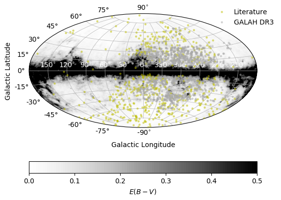
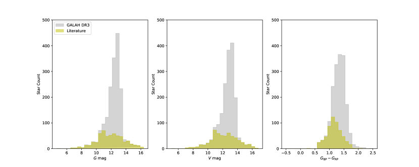
The stars from the RPE Initial Sample were then cross-matched with Gaia Early Data Release 3 (EDR3; Gaia Collaboration et al. 2021), using the same methods outlined in Shank et al. (2022b). Figure 1 shows the spatial distribution of these subsets of RPE stars in Galactic coordinates. A comparison of the magnitudes and colors for the RPE literature and GALAH DR3 subsets can be seen in Figure 2. From inspection of the figure, it is clear the GALAH DR3 subset of the RPE Initial Sample peaks at fainter magnitudes and redder colors compared to the literature RPE literature subset. RPE stars from the literature are relatively bright, due to the need for high-resolution spectra to detect the -process elements. Bright stars can be studied with smaller aperture telescopes, and require less observation time on larger aperture telescopes. GALAH DR3 (all spectra obtained with the AAT 3.9-m telescope) includes spectra taken for somewhat fainter stars.
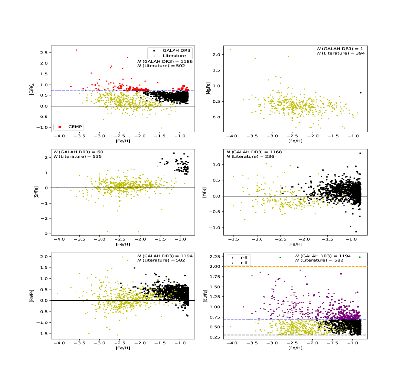
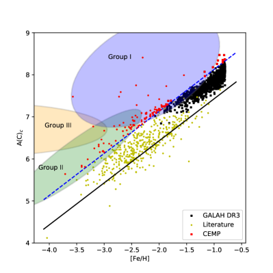
The available elemental-abundance ratio estimates for stars in the RPE Initial Sample are plotted in Figure 3, as a function of [Fe/H]. The RPE stars in GALAH DR3 do not offer much in terms of both Mg and Sr, and are included here for the sake of completeness. In the case of Sr, which is a first-peak -process element, Y can be used as a first-peak substitute with more elemental abundances readily available from GALAH DR3; there is no comparable element for Mg. While results using these elements are postulated, future studies will allow further revisions, where necessary, as the information on abundances is updated and expanded. Figure 4 provides histograms of the elemental-abundance ratios considered in the present work. As can be seen from inspection of these figures, stars in the RPE Initial Sample cover a wide range of abundances. This allows the abundance space to be accurately sub-sampled in later stages of our analysis. The Yoon-Beers Diagram of vs. [Fe/H] for these stars is shown in Figure 5; is the absolute carbon abundance444The standard definition for absolute abundance of an element X in a star () compared to the Sun () is . corrected from the observed value to account for the depletion of carbon on the giant branch, following Placco et al. (2014b). For the convenience of later research, the CEMP- stars are also provided in Table 14 of the Appendix. These stars are included in the analysis, with GALAH DR3 and Literature CEMP- stars. CEMP- stars are expected to be enriched in their birth clouds by external sources, and as such, do not conflict with the carbon-normal stars that dominate the RPE Initial Sample (Hansen et al., 2015). The RPE Initial Sample has -I stars, -II stars, and -III stars, for a total of RPE stars.
2.2 Construction of the Final Sample
2.2.1 Radial Velocities, Distances, and Proper Motions
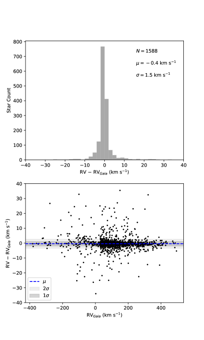
Radial velocities, parallaxes, and proper motions for each star are taken from Gaia EDR3, when available. Radial velocities are available for about of the RPE Initial Sample from Gaia EDR3, with typical errors of km s-1. The top panel of Figure 6 shows a histogram of the residual differences between the high-resolution radial velocities from the RPE Initial Sample and the Gaia EDR3 values. The biweight location and scale of these differences are km s-1 and km s-1, respectively. The bottom panel of this figure shows the residuals between the high-resolution sources and Gaia EDR3 radial velocities, as a function of the Gaia radial velocities. The blue dashed line is the biweight location, while the shaded regions represent the first (1) and second (2) biweight scale ranges.Gaia EDR3 radial velocities are used, when available, with literature values supplementing when not.
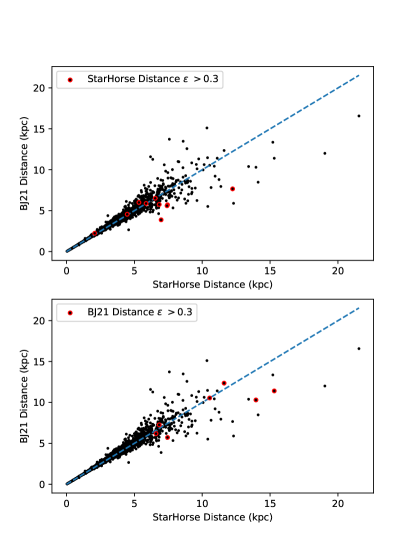
The distances to the stars are determined either through the StarHorse distance estimate (Anders et al., 2022) or the Bailer-Jones distance estimate (BJ21; Bailer-Jones et al. 2021). Parallax values in our RPE Initial Sample from EDR3 have an average error of mas. The BJ21 and StarHorse distances are determined by a Bayesian approach utilizing the EDR3 parallax, magnitude, and color (Bailer-Jones et al., 2021; Anders et al., 2022). The errors are presented for each star in the tables provided in the Appendix. Our adopted distances are chosen following the same procedure outlined in Shank et al. (2022a), though it is noted here that we prioritize Starhorse distances; the full procedure can be found in Table 12 in the Appendix. The proper motions in our RPE Initial Sample from Gaia EDR3 have an average error of as yr-1.
2.2.2 Dynamical Parameters
The orbital characteristics of the stars are determined using the Action-based GAlaxy Modelling Architecture555http://github.com/GalacticDynamics-Oxford/Agama (AGAMA) package (Vasiliev, 2019), using the same Solar positions and peculiar motions described in Shank et al. (2022b)666We adopt a Solar position of (, , ) kpc (GRAVITY Collaboration et al., 2020) and Solar peculiar motion in (U,W) as (,) km s-1 (Schönrich et al., 2010), with Galoctocentric Solar azimuthal velocity V km s-1 determined from Reid & Brunthaler (2020)., along with the same gravitational potential, MW2017 (McMillan, 2017). The D astrometric parameters, determined in Section 2, are run through the orbital integration process in AGAMA, in the same manner as Shank et al. (2022b), in order to calculate the orbital energy, cylindrical positions and velocities, angular momentum, cylindrical actions, and eccentricity. See Shank et al. (2022b) for definitions of these orbital parameters, and details of the Monte Carlo error calculation.
The RPE Initial Sample of stars was cut to exclude stars that are unbound from the MW () (J-, J-, and J-). Finally, in order to obtain accurate orbital dynamics, we conservatively remove stars with radial velocity differences km s-1 between the Gaia EDR3 values and the high-resolution source values. Most of these stars are expected to be binaries.
We also considered a cut to remove stars with [Ba/Eu] (rather than [Ba/Eu] ), in order to more confidently select stars with -process enhancement. We decided not to proceed with this cut, as ultimately including more stars with a wider range of [Ba/Eu] will only serve to increase the abundance dispersion when randomly sampled. Hence, this is a conservative choice; any stars that are included that are in fact not clearly RPE stars (i.e., they have contributions from, e.g., the -process) will only decrease the significance of our dispersion analysis described below777An explicit test of this cut indeed resulted in a small increase in the statistical significance of both Ba and Eu (with the exception of Eu for the -I sample), following the procedure described in Section 5..
Application of the above cuts leaves a total sample of stars to perform the following analysis. The dynamical parameters of the stars with orbits determined are listed in Table 13 in the Appendix; we refer to this as the RPE Final Sample. In the print edition, only the table description is provided; the full table is available only in electronic form.
| CDTG | Stars | Confidence | Associations with Previously Identified MW Substructure and Dynamical Groups |
|---|---|---|---|
| 1 | DS22a:DTG-15, DS22a:DTG-16 | ||
| 2 | GSE, IR18:E, DG21:CDTG-1, KH22:DTC-15, DS22b:DTG-7 | ||
| SL22:3, DS22a:DTG-22, EV21:NGC 4833, DS22b:DTG-27, GL21:DTG-37 | |||
| 3 | DS22b:DTG-1, DS22b:DTG-43 | ||
| 4 | GSE, DS22b:DTG-30, DG21:CDTG-13, DG21:CDTG-28, DS22a:DTG-18, GC21:Sausage, KH22:DTC-2 | ||
| 5 | GSE, AH17:VelHel-6, DG21:CDTG-9, DS22a:DTG-3, SL22:3 | ||
| 6 | Splashed Disk, DS22b:DTG-62, DG21:CDTG-5, DS22a:DTG-19 | ||
| 7 | MWTD, KH22:DTC-4, DS22b:DTG-14, DG21:CDTG-7, DS22b:DTG-99, DG21:CDTG-6, KM22:C-3, DS22b:DTG-97 | ||
| 8 | GSE, KH22:DTC-15, DS22b:DTG-57, DS22b:DTG-58, DG21:CDTG-18 | ||
| GL21:DTG-18, GC21:Sausage, DS22a:DTG-11, EV21:Ryu 879 (RLGC 2) | |||
| 9 | Splashed Disk, KH22:DTC-24, DG21:CDTG-25 | ||
| 10 | DS22b:DTG-5, DS22b:DTG-16 | ||
| 11 | GSE, EV21:NGC 5986, DG21:CDTG-29, KH22:DTC-19, EV21:NGC 6293, EV21:NGC 6402 (M 14) | ||
| 12 | GSE, DG21:CDTG-14, DS22b:DTG-78, KH22:DTC-10, KH22:DTC-13, GM17:Comoving, KH22:DTC-16, KM22:C-3 | ||
| 13 | DS22b:DTG-158 | ||
| 14 | KM22:C-3 | ||
| 15 | GSE, SM20:Sausage, GC21:Sausage, GL21:DTG-11, EV21:IC 1257 | ||
| 16 | new | ||
| 17 | Helmi Stream, DG21:CDTG-15, HK18:Green, NB20:H99, DS22b:DTG-42, SL22:60, GL21:DTG-3, GM18a:S2, GM18b:S2 | ||
| 18 | KH22:DTC-13, DS22b:DTG-4, KM22:C-3 | ||
| 19 | GSE, DG21:CDTG-10, KH22:DTC-2, SL22:6, DS22b:DTG-115, GC21:Sausage, GL21:DTG-24 | ||
| 20 | GSE, GL21:DTG-14, DS22b:DTG-12, DG21:CDTG-13, GM17:Comoving, GC21:Sausage, EV21:Ryu 879 (RLGC 2) | ||
| 21 | GSE, DS22b:DTG-18, DG21:CDTG-12 | ||
| 22 | Thamnos, DG21:CDTG-27, KH22:DTC-16, GC21:Sequoia, KM22:C-3 | ||
| 23 | Splashed Disk, AH17:VelHel-6, DG21:CDTG-11, DS22b:DTG-29 | ||
| 24 | GSE, DS22b:DTG-114 | ||
| 25 | LMS-1, DG21:CDTG-4, DS22b:DTG-67, GM18b:Cand10, GM18b:Cand11, GL21:DTG-2 | ||
| 26 | DS22b:DTG-121 | ||
| 27 | DG21:CDTG-18, KH22:DTC-13, KH22:DTC-17, DS22b:DTG-4, GM17:Comoving, KM22:Ophiuchus, KM22:C-3 | ||
| 28 | EV21:NGC 362, KH22:DTC-17, KH22:DTC-9, GM17:Comoving, KM22:C-3 | ||
| 29 | DS22a:DTG-32 | ||
| 30 | DG21:CDTG-23, KH22:DTC-24, DS22b:DTG-11 | ||
| 31 | new | ||
| 32 | GSE, DS22b:DTG-95, DS22b:DTG-8, SL22:3, GC21:Sausage, GL21:DTG-34 | ||
| 33 | GSE, GL21:DTG-23, DG21:CDTG-13, KH22:DTC-5, GM17:Comoving, GC21:Sausage, KH22:DTC-2, DS22a:DTG-10 | ||
| 34 | GSE, DG21:CDTG-21, KH22:DTC-3 | ||
| 35 | new | ||
| 36 | EV21:NGC 6397, DS22b:DTG-55, KH22:DTC-4, DS22a:DTG-9 |
Note. — We adopt the nomenclature for previously identified DTGs and CDTGs from Yuan et al. (2020a). For example, IR18:E is first initial then last initial of the first author (IR) (Roederer et al., 2018), the year the paper was published (18), and after the colon is the group obtained by the authors of the paper (E).
Note. — We use the following references for associations: AH17: Helmi et al. (2017), GM17: Myeong et al. (2017), HK18: Koppelman et al. (2018), GM18a: Myeong et al. (2018a), GM18b: Myeong et al. (2018b), IR18: Roederer et al. (2018), HL19: Li et al. (2019), SF19: Sestito et al. (2019), ZY19: Yuan et al. (2019), NB20: Borsato et al. (2020), HL20: Li et al. (2020), SM20: Monty et al. (2020), ZY20a: Yuan et al. (2020a), ZY20b: Yuan et al. (2020b), GC21: Cordoni et al. (2021), DG21: Gudin et al. (2021), CK21: Kielty et al. (2021), GL21: Limberg et al. (2021b), KH22: Hattori et al. (2022), KM22: Malhan et al. (2022), DS22a: Shank et al. (2022a), DS22b: Shank et al. (2022b), and SL22: Sofie Lövdal et al. (2022).
| NAME | [Fe/H] | [C/Fe]c | [Mg/Fe] | [Sr/Fe] | [Y/Fe] | [Ba/Fe] | [Eu/Fe] |
|---|---|---|---|---|---|---|---|
| CDTG- | |||||||
| Structure: Unassigned Structure | |||||||
| Group Assoc: DTG-15: Shank et al. (2022b) | |||||||
| Group Assoc: DTG-16: Shank et al. (2022b) | |||||||
| Stellar Assoc: No Stellar Associations | |||||||
| Globular Assoc: No Globular Associations | |||||||
| Dwarf Galaxy Assoc: No Dwarf Galaxy Associations | |||||||
| 140609001101322 | |||||||
| 170417004501188 | |||||||
| 170510003301241 | |||||||
| 160519003601012 | |||||||
| 160419003601272 | |||||||
| 140414004101079 | |||||||
| 160401004401264 | |||||||
| 160327005601145 | |||||||
| 170312001601291 | |||||||
| 150603002301086 | |||||||
| 140412002201386 | |||||||
| 140611001601101 | |||||||
| 150703002602272 | |||||||
| 170712002601049 | |||||||
| 140711001301278 | |||||||
| 150413004601222 | |||||||
| 160421005101363 | |||||||
| 180625004301097 | |||||||
| 150607005101057 | |||||||
| J204534.54143115.1 | |||||||
| 180604006201048 | |||||||
| 160817003101018 | |||||||
Note. — and represent the biweight estimates of the location and scale for the abundances in the CDTG.
Note. — This table is a stub; the full table is available in the electronic edition.
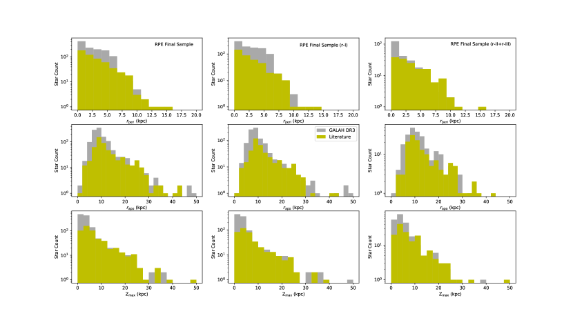
Figure 8 provides histograms of r (top), r (middle), and Z (bottom) for stars in the RPE Final Sample. The full sample is shown in the left column, -I stars are shown in the middle column, and -II and -III stars are shown in the right column. From inspection of this figure, it is clear that the majority of the stars in this sample occupy orbits that take them within the inner-halo region (up to around to kpc from the Galactic center), but they also explore regions well into the outer-halo region, up to kpc away from the Galactic plane. Although they appear rather similar, according to a Kolmogorov-Smirnov two-sample test between the -I (middle column) and -II plus -III (right column) distributions, the hypothesis that these two samples are drawn from the same parent population is rejected () for each of r (top), r (middle), and Z (bottom). It may be the case that this is due to the different masses of the dwarf satellites in which the -I and -II stars were formed (the majority of RPE stars are likely formed in dwarf satellites, but not all are required to be), but we choose not to speculate further on this point at present.
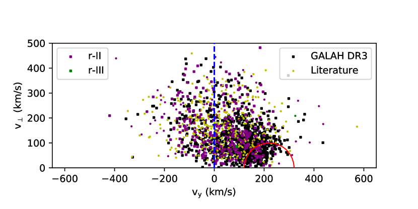
Figure 9 is the Toomre Diagram for the RPE Final Sample. The red solid semi-circle indicates whether a stellar orbit is disk-like (inside) or halo-like (outside). There are ( of) -I stars and ( of) -II stars that have disk-like kinematics. Of the disk-like -II stars, there are that are part of the GALAH DR3 subset of the RPE Final Sample, while the remaining eight are from the literature subset. This difference can be attributed to RPE stars being targeted more in the halo where they have a higher likelihood of detection; most known RPE stars reside in the halo (). The blue vertical dashed line indicates whether a stellar orbit is prograde (v km s-1) or retrograde (v km s-1). There are () -I stars and ( of) -II stars with prograde orbits. The Gudin et al. (2021) literature sample found an almost fifty-fifty split between RPE stars that have prograde orbits compared to retrograde orbits, while the expanded RPE Final Sample presented here has slightly more prograde stars ( or ) compared to retrograde stars. Note that simulations performed by Hirai et al. (2022) show that -II stars are slightly favored to be prograde as well. The RPE Final Sample has -I stars, -II stars, and -III stars, for a total of RPE stars.
3 Clustering Procedure
Helmi & de Zeeuw (2000) were among the first to suggest the use of integrals of motion, in their case orbital energies and angular momenta, to find substructure in the MW using the precision measurements of next-generation surveys that were planned at the time. McMillan & Binney (2008) considered the use of actions as a complement to the previously suggested orbital energy and angular momenta, with only the vertical angular momentum being invariant in an axisymmetric potential. Most recently, many authors have employed the orbital energies and cylindrical actions (E,Jr,Jϕ,Jz) to determine the substructure of the MW using Gaia measurements (Helmi et al., 2017; Myeong et al., 2018a, b; Roederer et al., 2018; Naidu et al., 2020; Yuan et al., 2020b, a; Gudin et al., 2021; Limberg et al., 2021b; Shank et al., 2022b).
As described in Shank et al. (2022b), we employ HDBSCAN in order to perform a cluster analysis over the orbital energies and cylindrical actions from the RPE Sample obtained through the procedure outlined in Section 2. The HDBSCAN algorithm888For a detailed description of the HDBSCAN algorithm visit: https://hdbscan.readthedocs.io/en/latest/how_hdbscan_works.html operates through a series of calculations that are able to separate the background noise from denser clumps of data in the dynamical parameters. We utilize the following parameters described in Shank et al. (2022b): min_cluster_size , min_samples , cluster_selection_method leaf , prediction_data True , Monte Carlo samples at , and minimum confidence set to .
Table 2 provides a listing of the Chemo-Dynamically Tagged Groups999Chemo-Dynamically Tagged Groups are derived from purely dynamical parameters. The chemical information comes from the RPE selection criteria, thus distinguishing them from Dynamically Tagged Groups (DTGs). (CDTGs) identified by this procedure, along with their numbers of member stars, confidence values (calculated as described in Shank et al. 2022b), and associations described below. Note that, although a minimum confidence value of was employed, the actual minimum value found for these CDTGs is (CDTG-15); only two other CDTGs have an assigned confidence value less than (CDTG-18 and CDTG-35). The average confidence level of the CDTGs is quite high, at . In total, there were stars ( of the Final Sample) assigned to the CDTGs.
The previously known groups are identified using the nomenclature introduced by Yuan et al. (2020a). For example, IR18:E refers to the first initial then the last initial of the lead author (IR) (Roederer et al., 2018), the year the paper was published (18), and after the colon is the group name provided by the authors of the paper (E). We use the following references for associations: AH17: Helmi et al. (2017), GM17: Myeong et al. (2017), HK18: Koppelman et al. (2018), GM18a: Myeong et al. (2018a), GM18b: Myeong et al. (2018b), IR18: Roederer et al. (2018), HL19: Li et al. (2019), SF19: Sestito et al. (2019), ZY19: Yuan et al. (2019), NB20: Borsato et al. (2020), HL20: Li et al. (2020), SM20: Monty et al. (2020), ZY20a: Yuan et al. (2020a), ZY20b: Yuan et al. (2020b), GC21: Cordoni et al. (2021), DG21: Gudin et al. (2021), CK21: Kielty et al. (2021), GL21: Limberg et al. (2021b), KH22: Hattori et al. (2022), KM22: Malhan et al. (2022), DS22a: Shank et al. (2022a), DS22b: Shank et al. (2022b), and SL22: Sofie Lövdal et al. (2022).
Table 3 lists the stellar members of the identified CDTGs, along with their values of [Fe/H], [C/Fe]c, [Mg/Fe], [Sr/Fe], [Y/Fe], [Ba/Fe], and [Eu/Fe], where available. The last line (in bold font) in the listing for each CDTG provides the mean and dispersion (both using biweight estimates) for each quantity. Note that for dynamical groups in which only fewer than three measurements of a given element are provided, we list the mean, and code the dispersion as a missing value.
Table 4 lists the derived dynamical parameters (and their errors) derived by AGAMA used in our analysis of the identified CDTGs.
4 Structure Associations
Associations between the newly identified CDTGs are now sought between known MW structures, including large-scale substructures101010Here, the term “large-scale substructure” is used to distinguish large over-densities of stars determined in the integral of motion space in the Galaxy, e.g., the substructures presented in Naidu et al. (2020)., previously identified dynamical groups, stellar associations, globular clusters, and dwarf galaxies.
| Cluster | Stars | (v,v,v) | (J,J,J) | E | ecc |
|---|---|---|---|---|---|
| (,,) | (,,) | ||||
| (km s-1) | (kpc km s-1) | (105 km2 s-2) | |||
| CDTG- | (,,) | (,,) | |||
| (,,) | (,,) | ||||
| CDTG- | (,,) | (,,) | |||
| (,,) | (,,) | ||||
| CDTG- | (,,) | (,,) | |||
| (,,) | (,,) | ||||
| CDTG- | (,,) | (,,) | |||
| (,,) | (,,) | ||||
| CDTG- | (,,) | (,,) | |||
| (,,) | (,,) | ||||
| CDTG- | (,,) | (,,) | |||
| (,,) | (,,) | ||||
| CDTG- | (,,) | (,,) | |||
| (,,) | (,,) | ||||
| CDTG- | (,,) | (,,) | |||
| (,,) | (,,) | ||||
| CDTG- | (,,) | (,,) | |||
| (,,) | (,,) | ||||
| CDTG- | (,,) | (,,) | |||
| (,,) | (,,) | ||||
| CDTG- | (,,) | (,,) | |||
| (,,) | (,,) | ||||
| CDTG- | (,,) | (,,) | |||
| (,,) | (,,) | ||||
| CDTG- | (,,) | (,,) | |||
| (,,) | (,,) | ||||
| CDTG- | (,,) | (,,) | |||
| (,,) | (,,) | ||||
| CDTG- | (,,) | (,,) | |||
| (,,) | (,,) | ||||
| CDTG- | (,,) | (,,) | |||
| (,,) | (,,) | ||||
| CDTG- | (,,) | (,,) | |||
| (,,) | (,,) | ||||
| CDTG- | (,,) | (,,) | |||
| (,,) | (,,) | ||||
| CDTG- | (,,) | (,,) | |||
| (,,) | (,,) | ||||
| CDTG- | (,,) | (,,) | |||
| (,,) | (,,) | ||||
| CDTG- | (,,) | (,,) | |||
| (,,) | (,,) | ||||
| CDTG- | (,,) | (,,) | |||
| (,,) | (,,) | ||||
| CDTG- | (,,) | (,,) | |||
| (,,) | (,,) | ||||
| CDTG- | (,,) | (,,) | |||
| (,,) | (,,) | ||||
| CDTG- | (,,) | (,,) | |||
| (,,) | (,,) | ||||
| CDTG- | (,,) | (,,) | |||
| (,,) | (,,) | ||||
| CDTG- | (,,) | (,,) | |||
| (,,) | (,,) | ||||
| CDTG- | (,,) | (,,) | |||
| (,,) | (,,) | ||||
| CDTG- | (,,) | (,,) | |||
| (,,) | (,,) | ||||
| CDTG- | (,,) | (,,) | |||
| (,,) | (,,) | ||||
| CDTG- | (,,) | (,,) | |||
| (,,) | (,,) | ||||
| CDTG- | (,,) | (,,) | |||
| (,,) | (,,) | ||||
| CDTG- | (,,) | (,,) | |||
| (,,) | (,,) | ||||
| CDTG- | (,,) | (,,) | |||
| (,,) | (,,) | ||||
| CDTG- | (,,) | (,,) | |||
| (,,) | (,,) | ||||
| CDTG- | (,,) | (,,) | |||
| (,,) | (,,) |
4.1 Milky Way Substructures
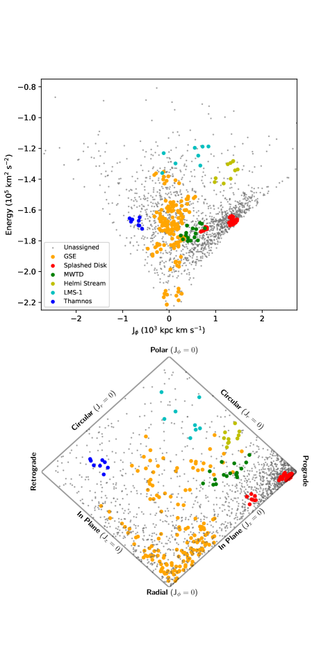
Analyzing the orbital energies and actions is insufficient to determine separate large-scale substructures. Information on the elemental abundances is crucial due to the differing star-formation histories of the structures, which can vary in both mass and formation redshift (Naidu et al., 2020). The outline for the prescription used to determine the structural associations with our CDTGs is described in Naidu et al. (2020), and explained in detail in Shank et al. (2022b). Simple selections are performed based on physically motivated choices for each substructure, excluding previously defined substructures, as the process iterates to decrease contamination between substructures. Following their procedures, we find six predominant MW substructures associated with our CDTGs, listed in Table 5. This table provides the numbers of stars, the mean and dispersion of their chemical abundances, and the mean and dispersion of their dynamical parameters for each substructure. The Lindblad Diagram and projected-action plot for these substructures is shown in Figure 10.
| MW Substructure | Stars | [Fe/H] | [C/Fe] | [Mg/Fe] | [Sr/Fe] | [Y/Fe] | [Ba/Fe] | [Eu/Fe] | (v,v,v) | (J,J,J) | E | ecc |
|---|---|---|---|---|---|---|---|---|---|---|---|---|
| (,,) | (,,) | |||||||||||
| (km s-1) | (kpc km s-1) | (105 km2 s-2) | ||||||||||
| GSE | 155 | (,,) | (,,) | |||||||||
| (,,) | (,,) | + | ||||||||||
| Splashed Disk | 36 | (,,) | (,,) | |||||||||
| (,,) | (,,) | + | ||||||||||
| MWTD | 16 | (,,) | (,,) | |||||||||
| (,,) | (,,) | + | ||||||||||
| Helmi Stream | 10 | (,,) | (,,) | |||||||||
| (,,) | (,,) | + | ||||||||||
| LMS-1 | 8 | (,,) | (,,) | |||||||||
| (,,) | (,,) | + | ||||||||||
| Thamnos | 8 | (,,) | (,,) | |||||||||
| (,,) | (,,) | + |
4.1.1 Gaia-Sausage-Enceladus
The most populated substructure identified here is Gaia-Sausage-Enceladus (GSE), which contains member stars across the associated CDTGs. The selection criteria for GSE is (Naidu et al., 2020). These CDTGs are distinct chemo-dynamical groups within GSE, as detected by previous authors as well, showing that, as a massive merger, GSE has distinct dynamical groupings within the progenitor satellite (Yuan et al., 2020a; Limberg et al., 2021b; Gudin et al., 2021; Sofie Lövdal et al., 2022). GSE is thought to be the remnant of an early merger that distributed a significant number of stars throughout the inner halo of the MW (Belokurov et al., 2018; Helmi et al., 2018). The action space determined for the member stars exhibits an extended radial component, a null azimuthal component within errors, and a null vertical component within errors. These orbital properties are the product of the high-eccentricity selection of the CDTGs, and agree with previous findings of GSE orbital characteristics when using other selection criteria (Koppelman et al., 2018; Myeong et al., 2018a; Limberg et al., 2021b, 2022).
The [Fe/H] of GSE found in our work () is rather metal poor, consistent with studies of its metallicity in other dynamical groupings, even though our sample contains more metal-rich stars that could have been associated with GSE (Gudin et al., 2021; Limberg et al., 2021b; Shank et al., 2022b). The stars that form CDTGs in GSE tend to favor the more metal-poor tail of the substructure, which is also seen in previous dynamical analysis. The [Mg/Fe] () of GSE exhibits a relatively low level, consistent with the low-Mg structure detected by Hayes et al. (2018) and with Mg levels consistent with accreted structures simulated by Mackereth et al. (2019), and explained through an accretion origin of GSE. We also obtain a [C/Fe] () for GSE; this elevated C level is indicative of being produced in Type II Supernovae, in agreement with the scenario put forth by Hasselquist et al. (2021) for GSE.
The RPE stars associated with GSE exhibit Eu enhancement on par with other detected MW susbtructures ([Eu/Fe]). Recently, Matsuno et al. (2021) and Naidu et al. (2021) tracked the formation of RPE stars in GSE, finding high levels of Eu present within identified GSE stars, consistent with the work presented here. Finally, we can associate the globular clusters Ryu 879 (RLGC2), IC 1257, NGC 4833, NGC 5986, NGC 6293, and NGC 6402 (M 14) with GSE, based on CDTGs with similar orbital characteristics and stellar associations of these globular clusters (see Sec. 4.3 for details). Note in Figure 10 how GSE occupies a large region of the Lindblad Diagram, concentrated in the planar and radial portions of the projected-action plot.
4.1.2 The Splashed Disk
The second-most populated substructure identified here is the Splashed Disk (SD), which contains member stars. The SD is thought to be a component of the primordial MW disk that was kinematically heated during the GSE merger event (Helmi et al., 2018; Di Matteo et al., 2019; Belokurov et al., 2020). The selection criteria for the SD is [/Fe][Fe/H] (Naidu et al., 2020). The mean velocity components of the SD are consistent with a null radial and vertical velocity, while showing a large positive azimuthal velocity consistent with disk-like stars. The mean eccentricity of these stars is most consistent with disk-like orbits. The SD is the most metal-rich substructure identified here ([Fe/H]). The high [Mg/Fe] () abundances for the SD shows that these stars are old, and they could be the result of a possible merger event, such as the merger between the MW and GSE progenitor, or heated from a primordial system present within the MW at the time of the GSE merger. The [C/Fe] () abundance for the SD is high, which is consistent with expectation from the high mean magnesium abundances as a tracer of Type II Supernovae in this substructure (Woosley & Weaver, 1995; Kobayashi et al., 2006).
Note that the SD overlaps with the Metal-Weak Thick Disk in the Lindblad Diagram (Figure 10). This is due to the selection criteria only using metallicity and Mg abundances to determine the SD stars (Naidu et al., 2020). Considering the SD is thought to be composed of stars that have been heated due to the GSE merger event, the positions of the SD stars in the Lindblad Diagram shows a relatively large deviation from disk-like orbits, though some seem to have certainly been less kinematically displaced.
4.1.3 The Metal-Weak Thick Disk
The third-most populated substructure identified here is the Metal-Weak Thick Disk (MWTD), which contains member stars. The MWTD is thought to have formed from either a merger scenario, possibly related to GSE, or the result of old stars born within the Solar radius migrating out to the Solar position due to tidal instabilities within the MW (Carollo et al., 2019). The selection criteria for the MWTD is [Fe/H], [/Fe], and J (Naidu et al., 2020). The relative lack of RPE stars in the MWTD agrees with simulations performed by Hirai et al. (2022), which show that the in situ component does not possess large numbers of highly enhanced -II stars ([Eu/Fe]). The non-existent radial and vertical velocity components, as well as the large positive azimuthal velocity component of the MWTD are all consistent with the velocity distribution for the MWTD from Carollo et al. (2019), even though the [Fe/H] cut in our dynamical analysis included more metal-rich stars than in their sample. The mean eccentricity distribution found within this substructure is also similar to that reported by Carollo et al. (2019), showing that the MWTD is a distinct component from the canonical thick disk (TD). Recently, both An & Beers (2020) and Dietz et al. (2021) have presented evidence that the MWTD is an independent structure from the TD.
The distribution in [Fe/H] () and mean velocity space represents a stellar population consistent with the high-Mg population (Hayes et al., 2018) ([Fe/H] ), with the mean Mg abundance ([Mg/Fe]) being similar within errors ([Mg/Fe] ). The [C/Fe] () abundance for the MWTD exhibits an enhancement in carbon, possibly pointing to a relation with the strongly prograde CEMP structure found in Dietz et al. (2021), which was attributed to the MWTD population. While this population is not explicitly recovered, there could be an overlap, and future studies will shed more light on this as new abundance information is explored.
Interestingly, the MWTD does not have many identified RPE stars compared to detections of this substructure in previous works that did not focus solely on RPE stars (Shank et al., 2022a, b). This could be due to the primordial MW disk not being enhanced in -process elements, shown for -II star simulations in Hirai et al. (2022), or a selection effect, with more stars with Mg abundances needing to be identified in the disk of the MW (note their are only stars with Mg abundances detected, which are needed to determine the MWTD substructure based on the procedure in Naidu et al. 2020). If future abundance measurements show that relatively few RPE stars are identified for the MWTD, then the formation scenarios of the primordial disk can be further constrained. Notice in Figure 10 how the MWTD occupies a lower energy component of the disk (the gray dots mostly positioned with prograde orbits) in the Lindblad Diagram, along with being in a more extended disk position as well, a selection which is seen in Naidu et al. (2020).
4.1.4 The Helmi Stream
| Structure | Reference | Associations | Identified CDTGs |
|---|---|---|---|
| MW Substructure | Naidu et al. (2020) | GSE | 2, 4, 5, 8, 11, 12, 15, 19, 20, 21, 24, 32, 33, 34 |
| Splashed Disk | 6, 9, 23 | ||
| Helmi Stream | 17 | ||
| LMS-1 | 25 | ||
| MWTD | 7 | ||
| Thamnos | 22 | ||
| Globular Clusters | Vasiliev & Baumgardt (2021) | Ryu 879 (RLGC 2) | 8, 20 |
| IC 1257 | 15 | ||
| NGC 362 | 28 | ||
| NGC 4833 | 2 | ||
| NGC 5986 | 11 | ||
| NGC 6293 | 11 | ||
| NGC 6397 | 36 | ||
| NGC 6402 (M 14) | 11 |
The third-least populated substructure identified here is the Helmi Stream (HS), which contains member stars. The HS is one of the first detected dynamical substructures in the MW using integrals of motions (Chiba & Yoshii, 1998; Helmi & White, 1999; Chiba & Beers, 2000). The selection criteria for the HS is J and L, with L (Naidu et al., 2020). The HS has a characteristically high vertical velocity, which separates it from other stars that lie in the disk, and can be seen in the sample here. The large uncertainty on the vertical velocity of the HS members corresponds to the positive and negative vertical velocity components of the stream, with the negative vertical velocity population dominating, consistent with the members determined here (Helmi, 2020).
The [Fe/H] of the HS is more metal poor in this sample ([Fe/H]), compared to the known HS members ([Fe/H] ; Koppelman et al. 2019a). However, Limberg et al. (2021a) recently noted that the metallicity range of HS is more metal poor than previously expected, with stars reaching [Fe/H] , which is consistent with both the study performed by Roederer et al. (2010) and the results presented here within errors. Limberg et al. (2021a) also considered -process abundances for the HS, showing that [Eu/Fe] () is larger over the wide range of metallicities ([Fe/H]), as also found for the stars reported in this work ([Eu/Fe] ). Notice in Figure 10 how the HS occupies a relatively isolated space in the Lindblad Diagram, thanks to the large vertical velocity of the stars providing the extra energy compared to the other disk stars.
4.1.5 LMS-1 (Wukong)
The second-least populated substructure identified here is LMS-1, which contains member stars. LMS-1 was first identified by Yuan et al. (2020a), and also detected by Naidu et al. (2020), who called it Wukong. The selection for LMS-1 is J, E, and [Fe/H] (Naidu et al., 2020). This structure is similar to GSE in terms of the velocity component, but is characterized by a higher energy along with a more metal-poor population (Naidu et al., 2020), also found for the small number of stars representing LMS-1 in our sample ([Fe/H]). The carbon and magnesium abundances are also high, which indicates an old population ([C/Fe] and [Mg/Fe]). LMS-1 exhibits low first-peak -process elements for both strontium and yttrium ([Sr/Fe] and [Y/Fe]). In Figure 10 LMS-1 has a higher energy compared to GSE in the Lindblad Diagram. However, these stars exhibit a lower eccentricity ( ecc ) compared to the GSE stars ( ecc ), forming their own distinct substructure, with a more clear division in the projected-action plot.
4.1.6 Thamnos
The Thamnos substructure also contains member stars. Thamnos was proposed by Koppelman et al. (2019b) as a merger event that populated stars in a retrograde orbit similar to thick-disk stars. The selection criteria for Thamnos is J, E, and [Fe/H] (Naidu et al., 2020). The low energy and strong retrograde rotation suggest that Thamnos merged with the MW long ago (Koppelman et al., 2019b). Here we find a similar low mean orbital energy and strong mean retrograde motion, and we recover as strong a retrograde motion as in Koppelman et al. (2019b), within errors. The low mean metallicity ([Fe/H]), consistent with the value reported by Limberg et al. (2021b) ([Fe/H]), and the elevated [C/Fe] () of these stars also supports the merger being ancient. The [Mg/Fe] () is high, also suggesting an old population, consistent with Kordopatis et al. (2020) ([Mg/Fe] ). As far as we are aware, this study presents the first known -process-element abundances detected in Thamnos, with [Eu/Fe] and [Ba/Fe], and shows that this old system was once subjected to multiple -process events, probably before being accreted into the Galaxy. Notice in Figure 10 how Thamnos occupies a space that could be described as a retrograde version of disk stars.
4.2 Associations to Previously Identified Groups and MW Substructure
Separately, we can compare the newly identified CDTGs in this work with other dynamical groups identified by previous authors in order to find structures in common. We take the mean group dynamical properties from the previously identified groups and compare them to the mean and dispersion for the dynamical parameters of our identified CDTGs. Stellar associations of are also considered, allowing the identification of stars in our sample that belong to previously identified groups. For details on the previous work used in this process, see Shank et al. (2022b). The resulting dynamical associations between our identified CDTGs and previously identified groups (along with substructure and globular cluster associations, see Section 4.3) are listed in Table 6. The previous groups that are associated to the identified CDTGs in this work are listed in Table 7. Table 3 lists the individual stellar associations for each of our CDTGs. The works that we use for previous groups are AH17: Helmi et al. (2017), GM17: Myeong et al. (2017), HK18: Koppelman et al. (2018), GM18a: Myeong et al. (2018a), GM18b: Myeong et al. (2018b), IR18: Roederer et al. (2018), HL19: Li et al. (2019), SF19: Sestito et al. (2019), ZY19: Yuan et al. (2019), NB20: Borsato et al. (2020), HL20: Li et al. (2020), SM20: Monty et al. (2020), ZY20a: Yuan et al. (2020a), ZY20b: Yuan et al. (2020b), GC21: Cordoni et al. (2021), DG21: Gudin et al. (2021), CK21: Kielty et al. (2021), GL21: Limberg et al. (2021b), KH22: Hattori et al. (2022), KM22: Malhan et al. (2022), DS22a: Shank et al. (2022a), DS22b: Shank et al. (2022b), and SL22: Sofie Lövdal et al. (2022). This work is distinguished from previous papers, thanks to the increase in RPE stars compared to Gudin et al. (2021), and preliminary abundance results for other elements such as Mg and Y. Select identified CDTGs related to each of the large-scale substructures described in Section 4.1 (along with one that is not associated to large-scale substructure) are examined in detail below.
4.2.1 CDTG-6
CDTG-6 is associated to the Splashed Disk (Naidu et al., 2020), and has interesting associations to previously identified groups. There are three stellar associations made between previously identified groups and CDTG-6, with two coming from DG21:CDTG-5111111We adopt the nomenclature for previously identified DTGs and CDTGs from Yuan et al. (2020a). For example, DG21:CDTG-5 is represented as the first initial then last initial of the first author (DG) (Gudin et al., 2021), followed by the year the paper was published (21), and after the colon is the group obtained by the authors of the paper (CDTG-5)., and one coming from DS22a:DTG-62 (Gudin et al., 2021; Shank et al., 2022a). DG21:CDTG-5 is associated to the MWTD by the authors (Gudin et al., 2021). DS22a:DTG-62 is not associated to any MW substructure by the authors, though it is noted that there were no measured -element abundances for the stars belonging to DS22a:DTG-62 (Shank et al., 2022a). CDTG-6 has three dynamical associations to previously identified groups – DG21:CDTG-5, DS22a:DTG-62, and DS22b:DTG-19 (Gudin et al., 2021; Shank et al., 2022a, b). DS22b:DTG-19 is associated to the MWTD by the authors (Shank et al., 2022b). CDTG-6 seems to point towards an association with either the MWTD or the Splashed Disk, but clearly more Mg abundances are needed before definitive claims can be made. While there were three studies (Gudin et al., 2021; Shank et al., 2022a, b) that had associations corresponding to the MWTD, Shank et al. (2022a) had limited -element abundance information.
4.2.2 CDTG-7
CDTG-7 is the only group associated to the MWTD following the procedure in Naidu et al. (2020). Three stellar associations are made to DG21:CDTG-7, two to KH22:DTC-4, and one each to DG21:CDTG-6, DS22a:DTG-14, and DS22a:DTG-99. DG21:CDTG-7 is associated to GSE by the authors, while DG21:CDTG-6 is not associated to MW substructure (Gudin et al., 2021). KH22:DTC-4 is not associated to any MW substructure, and is associated to IR18:C by the authors (Hattori et al., 2022). DS22a:DTG-14 is associated to the MWTD, with other associations to HL19:GL-1, DS22b:DTG-2, and DG21:CDTG-6 (Shank et al., 2022a). HL19:GL-1 is not associated to MW substructure by the authors, and also associated to AH17:VelHel-7 (Li et al., 2019). DS22b:DTG-2 is associated with the MWTD, and also associated to HL19:GL-1, DG21:CDTG-6, and DG21:CDTG-8, with DG21:CDTG-8 associated to the MWTD by the authors (Shank et al., 2022b; Gudin et al., 2021). DS22a:DTG-99 is not associated to any MW substructure, and also associated to HL19:GL-1 by the authors (Shank et al., 2022a). CDTG-7 is also dynamically associated to KM22:C-3 and DS22a:DTG-97 (Malhan et al., 2022; Shank et al., 2022a). KM22:C-3 is not associated to MW substructure by the authors, while DS22a:DTG97 is associated to GSE and also HL20:GR-1 (Malhan et al., 2022; Shank et al., 2022a). HL20:GR-1 is associated to AH17:VelHel-7, HL19:GL-1, and HL19:GL-2 by the authors, none of which are recovered here (Li et al., 2020). Interestingly, CDTG-7 has a few associations to GSE, but does not have a strong enough eccentricity ( ecc ) to be determined as GSE according to the procedure by Naidu et al. (2020) ( ecc ). The chemical information relates this more to the MWTD compared to GSE, with both [C/Fe] () and [Mg/Fe] () being more abundant in CDTG-7 compared to the detected abundances in GSE presented here ( and , respectively). In total, there are associations between CDTG-7 and previous works, with associations being related to the MWTD and to GSE by the previous authors, the rest were not associated to large-scale substructure.
4.2.3 CDTG-8
CDTG-8 is associated with GSE (Naidu et al., 2020), and has interesting associations to previously identified groups. Taking a closer look at CDTG-8, we have six stellar associations for CDTG-8 with two in KH22:DTC-15, and a star in each of GL21:DTG-18, DG21:CDTG-18, DS22a:DTG-57, and DS22a:DTG-58 (Limberg et al., 2021b; Gudin et al., 2021; Shank et al., 2022a). KH22:DTC-15 is associated to Pontus (Malhan et al., 2022), not discussed in this work, by the authors (Hattori et al., 2022). KH22:DTC-15 is associated to IR18:E, IR18:F, IR18:H, and ZY20a:DTG-38 by the authors as well (Hattori et al., 2022). ZY20a:DTG-38 is related to GSE by the authors (Yuan et al., 2020a). GL21:DTG-18 was not associated to GSE by the authors, or any MW substructure; however, it was associated to ZY20a:DTG-33, which was also not associated to any MW substructure by the authors (Limberg et al., 2021b; Yuan et al., 2020b). DG21:CDTG-18 was also not assigned to MW substructure by the authors, while DS22a:DTG-57, and DS22a:DTG-58 were associated to GSE (Gudin et al., 2021; Shank et al., 2022a). CDTG-8 is dynamically associated with GC21:Sausage, DS22a:DTG-57, and DS22b:DTG-11 which are all associated to GSE by their authors (Cordoni et al., 2021; Shank et al., 2022a, b). We also recover a globular cluster match with CDTG-8 to EV21:Ryu 879 (RLGC 2), which is typically associated with GSE dynamics (Callingham et al., 2022; Shank et al., 2022a, b). There are associations between CDTG-8 and previous groups, with being associated to GSE, to Pontus, and the rest not associated to large-scale substructure by the previous authors.
4.2.4 CDTG-17
Only one group is associated to the HS, CDTG-17. We can see that CDTG-17 has five stellar associations with DG21:CDTG-15, four with NB20:H99, four with SL22:60, three with HK18:Green, and one each with GL21:DTG-3 and DS22a:DTG-42 (Koppelman et al., 2018; Borsato et al., 2020; Gudin et al., 2021; Limberg et al., 2021b; Shank et al., 2022a; Sofie Lövdal et al., 2022). All of these groups were associated to the HS by their respective authors, with DG21:CDTG-15 also being associated to GL21:DTG-3 and ZY20a:DTG-3, of which we recover the GL21:DTG-3 association, and with ZY20a:DTG-3 being associated as HS members by the authors (Gudin et al., 2021; Limberg et al., 2021b; Yuan et al., 2020b). CDTG-17 is also dynamically associated to GM18a:S2, GM18b:S2, DG21:CDTG-15, GL21:DTG-3, and DS22a:DTG-42 which are all associated to HS by their authors (Myeong et al., 2018a, b; Gudin et al., 2021; Limberg et al., 2021b; Shank et al., 2022a). There are associations between CDTG-17 and previous groups, with all being assigned to the HS by the previous authors.
4.2.5 CDTG-22
CDTG-22 is associated to Thamnos. CDTG-22 has three stellar associations with two belonging in DG21:CDTG-27, which is identified as belonging to Thamnos by the authors (Gudin et al., 2021), and one belonging in KH22:DTC-16, which is associated to IR18:B by the authors (Hattori et al., 2022). On the other hand, CDTG-22 has a dynamical association to GC21:Sequoia, belonging to Sequoia according to the authors (Cordoni et al., 2021). However, Sequoia is a higher energy structure compared to Thamnos (Koppelman et al., 2019a). CDTG-22 also has a dynamical association to KM22:C-3, which is not associated by the authors (Malhan et al., 2022). This is a case where CDTG-22 could be between the two substructures of Thamnos and Sequoia in terms of energy, and more information is required before a definitive conclusion can be made. There are associations between CDTG-22 and previous groups, with 1 of those being associated with Thamnos, 1 being associated to Sequoia, and the other 2 not associated to large-scale substructure by the previous authors.
4.2.6 CDTG-25
CDTG-25 is associated to LMS-1 (Wukong) through the procedure outlined in Naidu et al. (2020). There were six stars from previously identified groups matched with CDTG-25 through a radius search of the CDTG-25 member stars. Three of the stars are in DG21:CDTG-4, and the other three are in DS22a:DTG-67. DG21:CDTG-4 is not assigned (Gudin et al., 2021; Shank et al., 2022a), while DS22a:DTG-67 is associated with LMS-1 (Yuan et al., 2020a). DG21:CDTG-4 was associated with GL21:DTG-2 by the authors, where Limberg et al. (2021b) made a tentative association with LMS-1. These associations seem to strengthen their argument for GL21:DTG-2. CDTG-25 is also dynamically associated with GM18b:Cand10, GM18b:Cand11, DG21:CDTG-4, GL21:DTG-2, and DS22a:DTG-67 (Myeong et al., 2018b; Gudin et al., 2021; Limberg et al., 2021b; Shank et al., 2022a). Both GM18b:Cand10 and GM18b:Cand11 were new groups identified by (Myeong et al., 2018b), though we note that LMS-1 was not discovered until two years later by Yuan et al. (2020a), meaning that LMS-1 was possibly detected through a dynamical search for groups. There are associations between CDTG-25 and previous groups, with being associated to LMS-1 and the other not associated to large-scale substructure by the previous authors.
| Reference | Associations | Identified CDTGs |
|---|---|---|
| Shank et al. (2022a) | DTG-4 | 18, 27 |
| DTG-1 | 3 | |
| DTG-5 | 10 | |
| DTG-7 | 2 | |
| DTG-8 | 32 | |
| DTG-11 | 30 | |
| DTG-12 | 20 | |
| DTG-14 | 7 | |
| DTG-16 | 10 | |
| DTG-18 | 21 | |
| DTG-27 | 2 | |
| DTG-29 | 23 | |
| DTG-30 | 4 | |
| DTG-42 | 17 | |
| DTG-43 | 3 | |
| DTG-55 | 36 | |
| DTG-57 | 8 | |
| DTG-58 | 8 | |
| DTG-62 | 6 | |
| DTG-67 | 25 | |
| DTG-78 | 12 | |
| DTG-95 | 32 | |
| DTG-97 | 7 | |
| DTG-99 | 7 | |
| DTG-114 | 24 | |
| DTG-115 | 19 | |
| DTG-121 | 26 | |
| DTG-158 | 13 | |
| Gudin et al. (2021) | CDTG-13 | 4, 20, 33 |
| CDTG-18 | 8, 27 | |
| CDTG-1 | 2 | |
| CDTG-4 | 25 | |
| CDTG-5 | 6 | |
| CDTG-6 | 7 | |
| CDTG-7 | 7 | |
| CDTG-9 | 5 | |
| CDTG-10 | 19 | |
| CDTG-11 | 23 | |
| CDTG-12 | 21 | |
| CDTG-14 | 12 | |
| CDTG-15 | 17 | |
| CDTG-21 | 34 | |
| CDTG-23 | 30 | |
| CDTG-25 | 9 | |
| CDTG-27 | 22 | |
| CDTG-28 | 4 | |
| CDTG-29 | 11 | |
| Hattori et al. (2022) | DTC-2 | 4, 19, 33 |
| DTC-13 | 12, 18, 27 | |
| DTC-4 | 7, 36 | |
| DTC-15 | 2, 8 | |
| DTC-16 | 12, 22 | |
| Hattori et al. (2022) | DTC-17 | 27, 28 |
| DTC-24 | 9, 30 | |
| DTC-3 | 34 | |
| DTC-5 | 33 | |
| DTC-9 | 28 | |
| DTC-10 | 12 | |
| DTC-19 | 11 | |
| Shank et al. (2022b) | DTG-3 | 5 |
| DTG-9 | 36 | |
| DTG-10 | 33 | |
| DTG-11 | 8 | |
| DTG-15 | 1 | |
| DTG-16 | 1 | |
| DTG-18 | 4 | |
| DTG-19 | 6 | |
| DTG-22 | 2 | |
| DTG-32 | 29 | |
| Limberg et al. (2021b) | DTG-2 | 25 |
| DTG-3 | 17 | |
| DTG-11 | 15 | |
| DTG-14 | 20 | |
| DTG-18 | 8 | |
| DTG-23 | 33 | |
| DTG-24 | 19 | |
| DTG-34 | 32 | |
| DTG-37 | 2 | |
| Myeong et al. (2018b) | Cand10 | 25 |
| Cand11 | 25 | |
| S2 | 17 | |
| Sofie Lövdal et al. (2022) | 3 | 2, 5, 32 |
| 6 | 19 | |
| 60 | 17 | |
| Cordoni et al. (2021) | Sausage | 4, 8, 15, 19, 20, 32, 33 |
| Sequoia | 22 | |
| Malhan et al. (2022) | C-3 | 7, 12, 14, 18, 22, 27, 28 |
| Ophiuchus | 27 | |
| Borsato et al. (2020) | H99 | 17 |
| Helmi et al. (2017) | VelHel-6 | 5, 23 |
| Koppelman et al. (2018) | Green | 17 |
| Monty et al. (2020) | Sausage | 15 |
| Myeong et al. (2017) | Comoving | 12, 20, 27, 28, 33 |
| Myeong et al. (2018a) | S2 | 17 |
| Roederer et al. (2018) | E | 2 |
4.2.7 CDTG-36
CDTG-36 is not assigned to any MW substructure, and has two stellar associations to DS22a:DTG-55, and one each with DS22b:DTG-9, KH22:DTC-4, and EV21:NGC 6397 (Vasiliev & Baumgardt, 2021; Hattori et al., 2022; Shank et al., 2022a, b). All of the past groups are not assigned by their authors to any large-scale MW substructure, with EV21:NGC 6397 being a globular cluster. KH22:DTC-4 is associated to IR18:C by the authors (Hattori et al., 2022). Both DS22a:DTG-55 and DS22b:DTG-9 are also associated with NGC 6397 as well. Although we have presented a stellar association, CDTG-36 has [Fe/H], as opposed to the metallicity of NGC 6397 of [Fe/H] (Jain et al., 2020). It is interesting to see stellar associations with NGC 6397 when the average metallicity of CDTG-36 does not compare to the metallicity of NGC 6397, and when both DS22a:DTG-55 and DS22b:DTG-9 are very metal poor ([Fe/H] and [Fe/H], respectively) (Shank et al., 2022a, b). There are associations between CDTG-36 and previous groups, with all not being assigned to large-scale substructure by the previous authors, though are associated to the globular cluster NGC 6397. CDTG-36 has 2 member stars which are very metal poor, while the other three are just metal poor, which may explain the discrepancy in metallicity observed between CDTG-36 and NGC 6397.
4.3 Globular Clusters and Dwarf Galaxies
Both globular clusters and dwarf galaxies have been shown to play an important role in the formation of stars that deviate from the usual chemical-abundance trends in the MW (Ji et al., 2016; Myeong et al., 2018c). Globular clusters can also be a good indicator of galaxy-formation history based on their metallicities and orbits (Woody & Schlaufman, 2021). From the work of Vasiliev & Baumgardt (2021), we can compare the dynamical properties of globular clusters to those of the CDTGs we identify. The procedure that is employed is the same one used for previously identified groups and stellar associations introduced in Sec. 4.2. The dynamics for dwarf galaxies of the MW (excluding the Large Magellanic Cloud, Small Magellanic Cloud, and Sagittarius) are also explored (McConnachie & Venn, 2020; Li et al., 2021). Shank et al. (2022b) contains details of the orbits of the globular clusters and dwarf galaxies. The same procedure used for previously identified groups was then applied to determine whether a CDTG was dynamically associated to the dwarf galaxy. Stellar associations were also determined for both globular clusters and dwarf galaxies in the same manner as previously identified groups.
The above comparison exercise led to seven of our identified CDTGs being associated to globular clusters. Table 6 provides a breakdown of which globular clusters are associated with our CDTGs. The CDTGs associated with globular clusters are expected to have formed in chemically similar birth environments; this is mostly supported through the similar chemical properties of the CDTGs. Associations of globular clusters with Galactic substructure have also been made by Massari et al. (2019) and Callingham et al. (2022).
Ryu 879 (RLGC 2) (CDTG-8 and CDTG-20), IC 1257 (CDTG-15), NGC 6293 (CDTG-11), and NGC 6402 (M 14) (CDTG-11) are dynamically associated to their respective groups. On the other hand, NGC 362 (CDTG-28), NGC 4833 (CDTG-2), NGC 5986 (CDTG-11), and NGC 6397 (CDTG-36) have stellar associations to their respective groups. Even though the matched stars in these globular clusters would have individually been associated with the globular cluster orbital parameters, the overall CDTG did not possess sufficiently similar orbital characteristics to be associated.
-
•
Ryu 879 (RLGC 2) has two dynamical CDTG associations that agree with each other in mean metallicity within errors ([Fe/H] for CDTG- vs. [Fe/H] for CDTG-), compared to the metallicity of Ryu 879 (RLGC 2) of [Fe/H] (Ryu & Lee, 2018). Both CDTG-9 and CDTG-20 are associated to GSE in this work, agreeing with the association to Galactic substructure of Ryu 879 (RLGC 2) by Callingham et al. (2022), while Massari et al. (2019) did not analyze Ryu 879 (RLGC 2), since the globular cluster was only recently discovered at the time of the publication.
- •
-
•
NGC 6293 is associated to the Bulge by both Massari et al. (2019) and Callingham et al. (2022), though this globular cluster is associated to GSE in this work. CDTG-11, which is associated to NGC 6293, interestingly has the lowest bound orbital energy (E), which actually overlaps with the potential energy of the defined bulge region in Callingham et al. (2022), but here CDTG-11 is assigned to GSE due to the large eccentricity (ecc). It is possible that this group formed in the bulge with intrinsically large eccentricity.
- •
- •
- •
- •
- •
We did not identify any associations of CDTGs to the sample of (surviving) MW dwarf galaxies, either through stellar associations, or through the dynamical association procedure described above. Note that we excluded known RPE stars that are members of recognized dwarf galaxies during the assembly of our field-star sample. As dwarf galaxy astrometric parameters themselves continue to improve, evidence may arise that shows some stripped stars after the dwarf has made a pass near the inner MW, but that is currently not seen in this sample. Nevertheless, some of the CDTGs identified by our analysis may well be associated with dwarf galaxies that have previously merged with the MW, and are now disrupted.
5 Chemical structure of identified CDTGs
5.1 Statistical Framework
Since the CDTGs we have obtained are expected to contain stars that (within each given CDTG) have been formed in similar primordial environments, the same processes may be responsible for their chemical enrichment. In this section we explore whether the elemental abundances of stars within the found CDTGs are more similar to each other than when the stars are randomly selected from the RPE Final Sample.
We follow the same statistical framework as outlined in Gudin et al. (2021). First, we use Monte Carlo sampling to select random groups of stars with a given measured elemental abundance (with ) from the sample and measure the biweight scale (Beers et al., 1990). This allows us to obtain empirical estimates of the cumulative distribution functions (CDFs) for the elemental-abundance dispersions within CDTGs of a given size. A low CDF value for a given elemental-abundance dispersion in a given CDTG indicates increased similarity for this species between the cluster member stars.
For the elemental-abundance dispersions selected at random for CDTGs of a given size, the probability of the number of clusters lying below a given CDF value (from 0 to 1) is described by the binomial distribution. Using three different CDF thresholds () and multiple different abundances (), we obtain overall statistical significances from multinomial distributions obtained by either grouping the cumulative probabilities across all values, or across all abundances. The overall statistical significance of the results is obtained by grouping the probabilities across both all values and all abundances. We denote these probabilities according to the following classification:
-
•
Individual Elemental-Abundance Dispersion (IEAD) probability: Individual binomial probability for specific values of and .
-
•
Full Elemental-Abundance Distribution (FEAD) probability: Multinomial probability for specific values of , grouped over all abundances .
-
•
Global Element Abundance Dispersion (GEAD) probability: Multinomial probability for specific abundances , grouped over all values of . This is the overall statistical significance for the particular abundance.
-
•
Overall Element Abundance Dispersion (OEAD) probability: Multinomial probability grouped over all values of and all abundances . This is the overall statistical significance of our clustering results.
For a more detailed discussion of the above probabilities, and their use, the interested reader is referred to Gudin et al. (2021).
| Cluster | Stars | [Fe/H] | [C/Fe]c | [Mg/Fe] | [Sr/Fe] | [Y/Fe] | [Ba/Fe] | [Eu/Fe] |
|---|---|---|---|---|---|---|---|---|
| CDTG- | ||||||||
| CDTG- | ||||||||
| CDTG- | ||||||||
| CDTG- | ||||||||
| CDTG- | ||||||||
| CDTG- | ||||||||
| CDTG- | ||||||||
| CDTG- | ||||||||
| CDTG- | ||||||||
| CDTG- | ||||||||
| CDTG- | ||||||||
| CDTG- | ||||||||
| CDTG- | ||||||||
| CDTG- | ||||||||
| CDTG- | ||||||||
| CDTG- | ||||||||
| CDTG- | ||||||||
| CDTG- | ||||||||
| CDTG- | ||||||||
| CDTG- | ||||||||
| CDTG- | ||||||||
| CDTG- | ||||||||
| CDTG- | ||||||||
| CDTG- | ||||||||
| CDTG- | ||||||||
| CDTG- | ||||||||
| CDTG- | ||||||||
| CDTG- | ||||||||
| CDTG- | ||||||||
| CDTG- | ||||||||
| CDTG- | ||||||||
| CDTG- | ||||||||
| CDTG- | ||||||||
| CDTG- | ||||||||
| CDTG- | ||||||||
| CDTG- | ||||||||
| Biweight (CDTG mean): | ||||||||
| Biweight (CDTG std): | ||||||||
| IQR (CDTG mean): | ||||||||
| IQR (CDTG std): | ||||||||
| Biweight (Final): | ||||||||
| IQR (Final): |
Note. — The first section of the table lists the biweight location and scale of the abundances for each of the CDTGs. The second section of the table lists the mean and the standard error of the mean (using biweight estimates) for both the location and scale of the abundances of the CDTGs, along with the IQR of the abundances of the CDTGs. The third section of the table lists the biweight location and scale of the Final Sample for each of the abundances, along with the IQR for each of the abundances in the Final Sample. The IQR lines are bolded to draw attention to the CDTG elemental-abundance mean IQRs to compare to the Final Sample abundance IQRs.
| Abundance | CDTGs | , , | IEAD Probabilities | GEAD Probabilities | OEAD Probability |
|---|---|---|---|---|---|
| [Fe/H] | 36 | , , | , , , | ||
| [C/Fe]c | 36 | , , | , , , | ||
| [Mg/Fe] | 12 | , , | , , , | ||
| [Sr/Fe] | 17 | , , | , , , | ||
| [Y/Fe] | 36 | , , | , , , | ||
| [Ba/Fe] | 36 | , , | , , , | ||
| [Eu/Fe] | 36 | , , | , , , | ||
| FEAD Probabilities | , , | ||||
Note. — The Individual Elemental-Abundance Dispersion (IEAD) probabilities represent the binomial probabilities for each element for the 0.5, 0.33, and 0.25, respectively. The Full Elemental-Abundance Dispersion (FEAD) probabilities represent the probabilities (across all elements) for the 0.5, 0.33, and 0.25, respectively. The Global Elemental-Abundance Dispersion (GEAD) probabilities represent the probabilities for the triplet of CDF levels for each element. The Overall Elemental-Abundance Dispersion (OEAD) probability represents the probability (across all elements) resulting from random draws from the full CDF. See text for details.
5.2 Important Caveats
Note that there are several caveats to the interpretation of this scheme that should be mentioned. Most importantly, a meaningful understanding of the derived probabilities (described below) depends on the contrast of the “typical” CDTG elemental-abundance dispersion to the abundance dispersion of the parent population to which it is compared, from which random draws are made. If the typical CDTG elemental-abundance dispersion is roughly commensurate with the dispersion of the parent sample, then by definition the dispersions will always be consistent with what are expected from the random draws, and one cannot expect the CDTG elemental-abundance dispersions to be significantly smaller. This requires that, in particular for a given element, prior to assessing the significance of its dispersion for a given set of CDTGs, we should compare its value to the expected value from the appropriate parent sample. We carry out this exercise, as described below, by inspection of the Inter-Quartile Range (IQR) for each element for a given set of CDTGs compared to the IQR of CDTGs drawn at random from the parent sample. As a rule of thumb, we demand that the IQR of the mean for each element of a set of CDTGs is on the order of one-half of the IQR of the parent-population CDTGs. Otherwise, there is insufficient “dynamical range” for the statistical inferences to be made with confidence, at least for individual elements.
Furthermore, as is perhaps obvious, the statistical power of our comparisons increase with the numbers of CDTGs in a given parent population. Thus, when we consider dynamical clusters formed exclusively from -II stars, as discussed below, it becomes more difficult to place confidence in the statistical inferences. For that reason, in the case of the clustering of -II stars, we have relaxed the criterion for the minimum number of stars per cluster to , rather than , more than doubling the numbers of identified -II CDTGs.
It should also be kept in mind that the observed CDTG elemental-abundance dispersions depend on a number of different parameters, including not only on the total mass of a given parent dwarf galaxy, but on its available gas mass for conversion into stars, the history of star formation in that environment, and the nature of the progenitor population(s) involved in the production of a given element. These are complex and interacting sets of conditions, and certainly are best considered in the context of simulations (such as Hirai et al. 2022). Consequently, the expected result for a given element in a given set of CDTGs is not always clear. However, we have designed our statistical tests to consider a broad set of questions of interest, the most pertinent of which for the current application are the FEAD and OEAD probabilities, which we employ for making our primary inferences.
| Abundance | CDTGs | , , | IEAD Probabilities | GEAD Probabilities | OEAD Probability |
|---|---|---|---|---|---|
| [Fe/H] | 28 | , , | , , , | ||
| [C/Fe]c | 28 | , , | , , , | ||
| [Mg/Fe] | 8 | , , | , , , | ||
| [Sr/Fe] | 12 | , , | , , , | ||
| [Y/Fe] | 27 | , , | , , , | ||
| [Ba/Fe] | 28 | , , | , , , | ||
| [Eu/Fe] | 28 | , , | , , , | ||
| FEAD Probabilities | , , | ||||
Note. — The Individual Elemental-Abundance Dispersion (IEAD) probabilities represent the binomial probabilities for each element for the 0.5, 0.33, and 0.25, respectively. The Full Elemental-Abundance Dispersion (FEAD) probabilities represent the probabilities (across all elements) for the 0.5, 0.33, and 0.25, respectively. The Global Elemental-Abundance Dispersion (GEAD) probabilities represent the probabilities for the triplet of CDF levels for each element. The Overall Elemental-Abundance Dispersion (OEAD) probability represents the probability (across all elements) resulting from random draws from the full CDF. See text for details.
5.3 Results
5.3.1 Full Sample of RPE CDTGs
Table 8 lists the means and dispersions of the elemental abundances explored in this study for each of the CDTGs identified in this work. The second part of the table lists the global CDTG properties, with the mean and standard error of the mean (using biweight location and scale) of both the CDTG means and dispersions being listed. The second part of the table also includes the IQR of the CDTG means and dispersions. The third part of the table lists the biweight location and scale of the elemental abundances in the Final Sample, along with the IQR of the elemental abundances in the Final Sample. As can be seen by comparing the two IQRs for each the CDTG results and the Final Sample, the IQRs for the CDTG results for 4 of the 7 elements considered are at least twice smaller, the exceptions being for [Fe/H] (which only slightly misses our rule of thumb), [Sr/Fe], and [Y/Fe]. The elements that meet the criteria, [C/Fe]c, [Mg/Fe], [Ba/Fe], and [Eu/Fe], provide stronger constraints compared to the ones that have large IQR ranges.
Table 9 lists the numbers of CDTGs with available estimates of the listed abundance ratios, and the numbers of CDTGs falling below the , , and levels of the CDFs, along with our calculated values for the various probabilities. The full and overall probabilities (captured by the FEAD and OEAD probability values) are very low, implying that the measured abundance spreads are highly statistically significant within our CDTGs across the entire sample; this is similar to the results found in Gudin et al. (2021) (see their Table 7). However, some of the individual abundance spreads (the GEAD probabilities) are not statistically significant, namely the [Mg/Fe] and [Sr/Fe] spreads. Keep in mind, as noted above, that the lack of contrast in the mean IQRs of [Fe/H], [Sr/Fe], and [Y/Fe] for our CDTGs with their corresponding mean IQRs for the full sample may impact interpretation of their probabilities.
By comparison, in Gudin et al. (2021), the [Fe/H], [C/Fe], [Sr/Fe], and [Ba/Fe] spreads were statistically significant, as inferred from their GEAD probabilities; the same is recovered in this study, with the exception of [Sr/Fe]. It should also be recalled that the sample of RPE stars considered by Gudin et al. is dominated by stars with lower [Fe/H] than our present sample, since the generally more metal-rich stars from GALAH were not available at that time.
Below we explore whether -I and -II stars exhibit different elemental-abundance patterns. For this purpose, we repeat the clustering procedure described in Section 3, separately for subsets of -I and -II stars. The result of this procedure is (-I) CDTGs ranging in size from to members and (-II) CDTGs ranging in size from to members, respectively. We then perform the same statistical analysis on each as described above.
| Abundance | CDTGs | , , | IEAD Probabilities | GEAD Probabilities | OEAD Probability |
|---|---|---|---|---|---|
| [Fe/H] | 20 | , , | , , , | ||
| [C/Fe]c | 19 | , , | , , , | ||
| [Mg/Fe] | 5 | , , | , , , | ||
| [Sr/Fe] | 10 | , , | , , , | ||
| [Y/Fe] | 17 | , , | , , , | ||
| [Ba/Fe] | 20 | , , | , , , | ||
| [Eu/Fe] | 20 | , , | , , , | ||
| FEAD Probabilities | , , | ||||
Note. — The Individual Elemental-Abundance Dispersion (IEAD) probabilities represent the binomial probabilities for each element for the 0.5, 0.33, and 0.25, respectively. The Full Elemental-Abundance Dispersion (FEAD) probabilities represent the probabilities (across all elements) for the 0.5, 0.33, and 0.25, respectively. The Global Elemental-Abundance Dispersion (GEAD) probabilities represent the probabilities for the triplet of CDF levels for each element. The Overall Elemental-Abundance Dispersion (OEAD) probability represents the probability (across all elements) resulting from random draws from the full CDF. See text for details.
5.3.2 The r-I Sample
The binomial statistics for the -I CDTGs are listed in Table 10. We observe a lack of statistical significance for the reduction of [Sr/Fe] and [Eu/Fe] abundance spreads, but other abundances (including [Mg/Fe], which exhibited a statistically insignificant spread reduction in the case of the full sample) exhibit statistically significant reductions in their spreads (all elements except for [Sr/Fe] and [Eu/Fe] have GEAD probabilities less than ).
From inspection of Table 17 in the Appendix, only 3 of the 7 elements considered ([Y/Fe], [Ba/Fe], and [Eu/Fe]) have contrasts in their mean CDTG IQRs relative to the mean IQRs of the full sample of -I stars that pass our factor of two rule of thumb (although [Fe/H] and [C/Fe] only narrowly miss), so interpretation of the GEAD probabilities for several of these elements should be regarded with caution.
The FEAD probabilities for the -I CDTGs are low, and are statistically significant for all three of the , and levels. The OEAD probability is highly statistically significant.
5.3.3 The r-II Sample
If we adopt the minimum number of stars per -II CDTG for the clustering exercise as we have for the full sample () and the -I sample (), we are left with only a total of -II CDTGs for the statistical analysis. We judge this to be too small, as experience suggests that a minimum of CDTGs provide the most stable results. Thus, we chose to reduce the minimum number of stars in order to form an -II CDTG from to . This increases the number of -II CDTGs from to , comparable to that in the full and the -I samples ( and respectively).
Table 11 shows the binomial statistics for our -II CDTGs. From inspection, the GEAD probabilities for the elements considered are statistically significant in the same manner as the Final Sample, with [Mg/Fe] and [Sr/Fe] both lacking stastical significance.
From inspection of Table 20 in the Appendix, only of the elements considered ([Y/Fe] and [Ba/Fe]) have mean IQRs for the -II CDTGs that are at least twice smaller than the mean IQR of the final sample, although [C/Fe] only narrowly misses our rule of thumb. Thus we can assume that, for many of the individual elements, there is not a useful dynamical range for confident interpretation for most of the GEADs.
The FEAD probabilities for the -II CDTGs are statistically significant for all three , , and levels. The OEAD probability is highly statistically significant.
6 Summary
We have assembled an RPE Initial Sample of stars ( -I stars, -II stars, and -III stars) from both a literature search and GALAH DR3 (Buder et al., 2021) survey data, with stars that met the -process-enhancement requirements listed in Table 1. A total of of these stars are identified as CEMP- stars; these are listed in Table 14 in the Appendix. These stars are of interest due to their enhanced carbon abundance and association to the morphological groups described in Yoon et al. (2016). Based on their classification scheme, there are Group I CEMP- stars, Group II CEMP- stars, and Group III CEMP- stars, with a number of stars that have ambiguous classifications. This list provides a useful reference for high-resolution follow-up targets, some of which has already begun (e.g., Rasmussen et al. 2020 and Zepeda et al. 2022).
The RPE Final Sample of stars ( -I stars, -II stars, and -III stars) had radial velocity and astrometric information from which orbits were constructed, in order to identify Chemo-Dynamically Tagged Groups (CDTGs) in orbital energy and cylindrical action space with the HDBSCAN algorithm. We chose HDBSCAN as the clustering algorithm due to precedence within the literature (Koppelman et al., 2019b; Gudin et al., 2021; Limberg et al., 2021b; Shank et al., 2022b), and its ability to extract clusters of stars over the energy and action space.
We recover CDTGs that include between and members, with CDTGs containing at least member stars. These CDTGs were associated with MW substructures, resulting in the re-identification of the Gaia-Sausage-Enceladus, the Splashed Disk, the Metal-Weak Thick Disk, the Helmi Stream, LMS-1 (Wukong), and Thamnos. A total of CDTGs were associated with globular clusters, while no surviving dwarf galaxies were determined to be associated with the identified CDTGs. Previously identified groups were found to be associated with the CDTGs as well, with past work mostly confirming our substructure identification, and showing some limitations in the procedure, which we discussed. Each of these associations allow insights into the dynamical and chemical properties of the parent substructures.
The implications of past group and stellar associations were explored, with emphasis placed on the structure associations. Stellar associations to stars with abnormal MW abundances were addressed as being good candidates for high-resolution follow-up spectroscopy targets, due to the statistical likelihood of the other members being chemically peculiar as well, mostly focused on RPE and CEMP stars.
We have considered the statistical significance of the elemental-abundance dispersions across the identified RPE CDTGs for a set of seven abundance ratios ([Fe/H]], [C/Fe], [Mg/Fe], [Sr/Fe], [Y/Fe], [Ba/Fe], and [Eu/Fe]). CDTGs are statistically examined, in order to assess the similarity (or not) of the chemical-evolution histories in their presumed dwarf-galaxy birth environments, following the approach developed by Gudin et al. (2021). We point out that, for a number of elements considered, the mean IQRs of the dispersions in the CDTGs do not provide sufficient dynamical range compared to the mean IQR of the parent samples with which they are compared (we suggest they must be a factor of two smaller) in order to enable meaningful interpretations of the Global Elemental-Abundance (GEAD) probabilities.
However, the probabilities that consider the distributions of all of the elements across the CDFs for the set of CDTGs (the Full Elemental-Abundance Distribution, FEAD probabilities, and the Overall Elemental-Abundance Distribution, OEAD probablities), strongly support the assertion that the stars associated with individual RPE CDTGs indeed share similar chemical-enrichment histories, as previously claimed by Gudin et al. (2021). We have also divided the full sample into RPE stars classified as moderately -process enhanced (-I) and highly -process enhanced (-II), and find similar results.
The methods presented here will be used in future samples that contain many more RPE stars, especially with planned data releases from the RPA increasing their total number, and other ongoing or planned surveys allowing for a systematic search for RPE stars. The next steps in advancing our understanding of the birth environments and the nature of the astrophysical site(s) of the -process require detailed comparisons with modern high-resolution (spatial and temporal) simulations of the formation of Milky Way-like galaxies, along the lines explored by Hirai et al. (2022).
7 Appendix
Here we present the table for the RPE Initial Sample (Table 12) and the RPE Final Sample (Table 13). In the print edition, only the table descriptions are provided; the full tables are available only in electronic form.
We also present Table 14, which describes the identified CEMP- stars and their associated morphological groups, according to the regions defined by Yoon et al. (2016). Tables 15 and 16 show the CDTGs identified by HDBSCAN and the CDTG dynamical parameters as determined by AGAMA for the -I Sample, respectively. Table 17 lists the means and dispersions of the CDTGs identified in the -I Sample, along with the statistics on all the CDTGs and the -I Sample. Tables 18 and 19 show the CDTGs identified by HDBSCAN and the CDTG dynamical parameters as determined by AGAMA for the -II Sample, respectively. Table 20 lists the means and dispersions of the CDTGs identified in the -II Sample, along with the statistics on all the CDTGs and the -II Sample.
| Column | Field | Unit | Description |
|---|---|---|---|
| 1 | Name | The name of the star as given by the Reference | |
| 2 | Source ID | The Gaia EDR3 Source ID of the star | |
| 3 | RA | (J2000) | The Right Ascension of the star given in hours:minutes:seconds |
| 4 | DEC | (J2000) | The Declination of the star given in degrees:minutes:seconds |
| 5 | The magnitude of the star as given by the Reference | ||
| 6 | The Gaia mean magnitude of the star as given by the Gaia Source ID | ||
| 7 | The Gaia BP RP color mean magnitude of the star as given by the Gaia Source ID | ||
| 8 | (Gaia) | The magnitude of the star as determined by the transformations from G mag to V mag using | |
| given by Riello et al. (2021) | |||
| 9 | RV | (km s-1) | The radial velocity as given by RV Reference |
| 10 | Error | (km s-1) | The radial velocity error as given by RV Reference |
| 11 | RVGaia | (km s-1) | The radial velocity as given by the Gaia Source ID |
| 12 | Error | (km s-1) | The radial velocity error as given by the Gaia Source ID |
| 13 | Parallax | (mas) | The parallax as given by the Gaia Source ID |
| 14 | Error | (mas) | The parallax error as given by the Gaia Source ID |
| 15 | Distance | (kpc) | The inverse parallax distance (1/Parallax) |
| 16 | Error | (kpc) | The inverse parallax distance error (Parallaxerror/(Parallax2)) |
| 17 | DistanceCorrected | (kpc) | The corrected inverse parallax distance (1/(Parallax + 0.026)) based on Huang et al. (2021) |
| 18 | Error | (kpc) | The corrected inverse parallax distance error (Parallaxerror/((Parallax + 0.026)2)) |
| based on Huang et al. (2021) | |||
| 19 | Relative Error | The relative error of the corrected distance as given by Gaia | |
| 20 | Distance BJ21 | (kpc) | The 50 percentile distance as given by Bailer-Jones et al. (2021) based on the Gaia Source ID |
| 21 | Error | (kpc) | The 50 percentile error as estimated by the 84 percentile distance and the 16 percentile |
| distance as given by Bailer-Jones et al. (2021) based on the Gaia Source ID ((dist84-dist16)/2) | |||
| 22 | Relative Error | The relative error of the 50 percentile distance as given by Bailer-Jones et al. (2021) based on | |
| the Gaia Source ID | |||
| 23 | Distance StarHorse | (kpc) | The 50 percentile distance as given by Anders et al. (2022) based on the Gaia Source ID |
| 24 | Error | (kpc) | The 50 percentile error as estimated by the 84 percentile distance and the 16 percentile |
| distance as given by Anders et al. (2022) based on the Gaia Source ID ((dist84-dist16)/2) | |||
| 25 | Relative Error | The relative error of the 50 percentile distance as given by Anders et al. (2022) based on the | |
| Gaia Source ID | |||
| 26 | PMRA | (mas yr-1) | The proper motion in the Right Ascension as given by the Gaia Source ID |
| 27 | Error | (mas yr-1) | The proper motion error in the Right Ascension as given by the Gaia Source ID |
| 28 | PMDEC | (mas yr-1) | The proper motion in the Declination as given by the Gaia Source ID |
| 29 | Error | (mas yr-1) | The proper motion error in the Declination as given by the Gaia Source ID |
| 30 | Correlation Coefficient | The correlation coefficient between the proper motion in Right Ascension and the proper motion | |
| in Declination as given by the Gaia Source ID | |||
| 31 | Teff | (K) | The effective temperature of the star as given by the Reference |
| 32 | log g | (cgs) | The surface gravity of the star as given by the Reference |
| 33 | [Fe/H] | The metallicity of the star as given by (log (Fe) - log (Fe)⊙) | |
| (Solar value of 7.50 taken from Asplund et al. (2009)) | |||
| 34 | log (Fe) | The logarithmic iron abundance of the star as given by the Reference | |
| 35 | [C/Fe] | The carbon abundance ratio of the star as given by (log (C) - log | |
| (C)⊙ - [Fe/H]) (Solar value of 8.43 taken from Asplund et al. (2009)) | |||
| 36 | log (C) | The logarithmic carbon abundance of the star as given by the Reference | |
| 37 | [C/Fe]c | The carbon abundance ratio corrected for evolutionary effects from Placco et al. (2014b) | |
| 38 | ACc | The absolute carbon corrected for evolutionary effects from Placco et al. (2014b) ([C/Fe]c | |
| + [Fe/H] + log (C)⊙) (Solar value of 8.43 taken from Asplund et al. (2009)) | |||
| 39 | CARDET | Flag with “D” if the carbon abundance ratio ([C/Fe]) is detected by Reference and “U” if an | |
| upper limit by Reference and “L” if a lower limit by Reference and “X” if none is detected | |||
| by Reference | |||
| 40 | CEMP | Flag as “C” for Carbon-Enhanced Metal-Poor (CEMP) if [C/Fe]c and “I” for | |
| CEMP-intermediate if [C/Fe]c and “N” for Carbon-Normal if | |||
| [C/Fe]c and “X” if there is no [C/Fe]c information | |||
| 41 | [Mg/Fe] | The magnesium abundance ratio of the star as given by (log (Mg) - log | |
| (Mg)⊙ - [Fe/H]) (Solar value of 7.60 taken from Asplund et al. (2009)) | |||
| 42 | log (Mg) | The logarithmic magnesium abundance of the star as given by the Reference | |
| 43 | MAGDET | Flag with “D” if the magnesium abundance ratio ([Mg/Fe]) is detected by Reference and “U” if | |
| an upper limit by Reference and “L” if a lower limit by Reference and “X” if none is | |||
| detected by Reference | |||
| 44 | [Sr/Fe] | The strontium abundance ratio of the star as given by (log (Sr) - log | |
| (Sr)⊙ - [Fe/H]) (Solar value of 2.87 taken from Asplund et al. (2009)) | |||
| 45 | log (Sr) | The logarithmic strontium abundance of the star as given by the Reference | |
| 46 | STRDET | Flag with “D” if the strontium abundance ratio ([Sr/Fe]) is detected by Reference and “U” if | |
| an upper limit by Reference and “L” if a lower limit by Reference and “X” if none is | |||
| detected by Reference | |||
| 47 | [Y/Fe] | The yttrium abundance ratio of the star as given by (log (Y) - log | |
| (Y)⊙ - [Fe/H]) (Solar value of 2.21 taken from Asplund et al. (2009)) | |||
| 48 | log (Y) | The logarithmic yttrium abundance of the star as given by the Reference | |
| 49 | YTTDET | Flag with “D” if the yttrium abundance ratio ([Y/Fe]) is detected by Reference and “U” if an | |
| upper limit by Reference and “L” if a lower limit by Reference and “X” if none is detected | |||
| by Reference | |||
| 50 | [Ba/Fe] | The barium abundance ratio of the star as given by (log (Ba) - log | |
| (Ba)⊙ - [Fe/H]) (Solar value of 2.18 taken from Asplund et al. (2009)) | |||
| 51 | log (Ba) | The logarithmic barium abundance of the star as given by the Reference | |
| 52 | BARDET | Flag with “D” if the barium abundance ratio ([Ba/Fe]) is detected by Reference and “U” if an | |
| upper limit by Reference and “L” if a lower limit by Reference and “X” if none is detected | |||
| by Reference | |||
| 53 | [Eu/Fe] | The europium abundance ratio of the star as given by (log (Eu) - log | |
| (Eu)⊙ - [Fe/H]) (Solar value of 0.52 taken from Asplund et al. (2009)) | |||
| 54 | log (Eu) | The logarithmic europium abundance of the star as given by the Reference | |
| 55 | EURDET | Flag with “D” if the europium abundance ratio ([Eu/Fe]) is detected by Reference and “U” if | |
| an upper limit by Reference and “L” if a lower limit by Reference and “X” if none is | |||
| detected by Reference | |||
| 56 | Class | The class for the star, as given by Table 1 | |
| 57 | SNR | The average Signal-to-Noise Ratio of the spectrum as given by the Reference | |
| 58 | Reference | The Reference for the star | |
| 59 | Reference | The Reference for the V magnitude of the star | |
| 60 | Distance AGAMA | The Reference for the distance used in AGAMA (StarHorse prioritized over BJ21 unless StarHorse | |
| distance has relative error greater than 0.3, if both have a relative error greater than 0.3 | |||
| we adopt no distance estimate) | |||
| 61 | RV Reference | The Reference for the RV |
| Column | Field | Unit | Description |
|---|---|---|---|
| 1 | Name | The name of the star as given by the Reference | |
| 2 | Source ID | The Gaia EDR3 Source ID of the star | |
| 3 | RA | (J2000) | The Right Ascension of the star given in hours:minutes:seconds |
| 4 | DEC | (J2000) | The Declination of the star given in degrees:minutes:seconds |
| 5 | The magnitude of the star as given by the Reference | ||
| 6 | The Gaia mean magnitude of the star as given by the Gaia Source ID | ||
| 7 | The Gaia BP RP color mean magnitude of the star as given by the Gaia Source ID | ||
| 8 | (Gaia) | The magnitude of the star as determined by the transformations from G mag to V mag using | |
| given by Riello et al. (2021) | |||
| 9 | RV | (km s-1) | The radial velocity as given by RV Reference |
| 10 | Error | (km s-1) | The radial velocity error as given by RV Reference |
| 11 | RVGaia | (km s-1) | The radial velocity as given by the Gaia Source ID |
| 12 | Error | (km s-1) | The radial velocity error as given by the Gaia Source ID |
| 13 | Parallax | (mas) | The parallax as given by the Gaia Source ID |
| 14 | Error | (mas) | The parallax error as given by the Gaia Source ID |
| 15 | Distance | (kpc) | The inverse parallax distance (1/Parallax) |
| 16 | Error | (kpc) | The inverse parallax distance error (Parallaxerror/(Parallax2)) |
| 17 | DistanceCorrected | (kpc) | The corrected inverse parallax distance (1/(Parallax + 0.026)) based on Huang et al. (2021) |
| 18 | Error | (kpc) | The corrected inverse parallax distance error (Parallaxerror/((Parallax + 0.026)2)) |
| based on Huang et al. (2021) | |||
| 19 | Relative Error | The relative error of the corrected distance as given by Gaia | |
| 20 | Distance BJ21 | (kpc) | The 50 percentile distance as given by Bailer-Jones et al. (2021) based on the Gaia Source ID |
| 21 | Error | (kpc) | The 50 percentile error as estimated by the 84 percentile distance and the 16 percentile |
| distance as given by Bailer-Jones et al. (2021) based on the Gaia Source ID ((dist84-dist16)/2) | |||
| 22 | Relative Error | The relative error of the 50 percentile distance as given by Bailer-Jones et al. (2021) based on | |
| the Gaia Source ID | |||
| 23 | Distance StarHorse | (kpc) | The 50 percentile distance as given by Anders et al. (2022) based on the Gaia Source ID |
| 24 | Error | (kpc) | The 50 percentile error as estimated by the 84 percentile distance and the 16 percentile |
| distance as given by Anders et al. (2022) based on the Gaia Source ID ((dist84-dist16)/2) | |||
| 25 | Relative Error | The relative error of the 50 percentile distance as given by Anders et al. (2022) based on the | |
| Gaia Source ID | |||
| 26 | PMRA | (mas yr-1) | The proper motion in the Right Ascension as given by the Gaia Source ID |
| 27 | Error | (mas yr-1) | The proper motion error in the Right Ascension as given by the Gaia Source ID |
| 28 | PMDEC | (mas yr-1) | The proper motion in the Declination as given by the Gaia Source ID |
| 29 | Error | (mas yr-1) | The proper motion error in the Declination as given by the Gaia Source ID |
| 30 | Correlation Coefficient | The correlation coefficient between the proper motion in Right Ascension and the proper motion | |
| in Declination as given by the Gaia Source ID | |||
| 31 | Teff | (K) | The effective temperature of the star as given by the Reference |
| 32 | log g | (cgs) | The surface gravity of the star as given by the Reference |
| 33 | [Fe/H] | The metallicity of the star as given by (log (Fe) - log (Fe)⊙) | |
| (Solar value of 7.50 taken from Asplund et al. (2009)) | |||
| 34 | log (Fe) | The logarithmic iron abundance of the star as given by the Reference | |
| 35 | [C/Fe] | The carbon abundance ratio of the star as given by (log (C) - log | |
| (C)⊙ - [Fe/H]) (Solar value of 8.43 taken from Asplund et al. (2009)) | |||
| 36 | log (C) | The logarithmic carbon abundance of the star as given by the Reference | |
| 37 | [C/Fe]c | The carbon abundance ratio corrected for evolutionary effects from Placco et al. (2014b) | |
| 38 | ACc | The absolute carbon corrected for evolutionary effects from Placco et al. (2014b) ([C/Fe]c | |
| + [Fe/H] + log (C)⊙) (Solar value of 8.43 taken from Asplund et al. (2009)) | |||
| 39 | CARDET | Flag with “D” if the carbon abundance ratio ([C/Fe]) is detected by Reference and “U” if an | |
| upper limit by Reference and “L” if a lower limit by Reference and “X” if none is detected | |||
| by Reference | |||
| 40 | CEMP | Flag as “C” for Carbon-Enhanced Metal-Poor (CEMP) if [C/Fe]c and “I” for | |
| CEMP-intermediate if [C/Fe]c and “N” for Carbon-Normal if | |||
| [C/Fe]c and “X” if there is no [C/Fe]c information | |||
| 41 | [Mg/Fe] | The magnesium abundance ratio of the star as given by (log (Mg) - log | |
| (Mg)⊙ - [Fe/H]) (Solar value of 7.60 taken from Asplund et al. (2009)) | |||
| 42 | log (Mg) | The logarithmic magnesium abundance of the star as given by the Reference | |
| 43 | MAGDET | Flag with “D” if the magnesium abundance ratio ([Mg/Fe]) is detected by Reference and “U” if | |
| an upper limit by Reference and “L” if a lower limit by Reference and “X” if none is | |||
| detected by Reference | |||
| 44 | [Sr/Fe] | The strontium abundance ratio of the star as given by (log (Sr) - log | |
| (Sr)⊙ - [Fe/H]) (Solar value of 2.87 taken from Asplund et al. (2009)) | |||
| 45 | log (Sr) | The logarithmic strontium abundance of the star as given by the Reference | |
| 46 | STRDET | Flag with “D” if the strontium abundance ratio ([Sr/Fe]) is detected by Reference and “U” if | |
| an upper limit by Reference and “L” if a lower limit by Reference and “X” if none is | |||
| detected by Reference | |||
| 47 | [Y/Fe] | The yttrium abundance ratio of the star as given by (log (Y) - log | |
| (Y)⊙ - [Fe/H]) (Solar value of 2.21 taken from Asplund et al. (2009)) | |||
| 48 | log (Y) | The logarithmic yttrium abundance of the star as given by the Reference | |
| 49 | YTTDET | Flag with “D” if the yttrium abundance ratio ([Y/Fe]) is detected by Reference and “U” if an | |
| upper limit by Reference and “L” if a lower limit by Reference and “X” if none is detected | |||
| by Reference | |||
| 50 | [Ba/Fe] | The barium abundance ratio of the star as given by (log (Ba) - log | |
| (Ba)⊙ - [Fe/H]) (Solar value of 2.18 taken from Asplund et al. (2009)) | |||
| 51 | log (Ba) | The logarithmic barium abundance of the star as given by the Reference | |
| 52 | BARDET | Flag with “D” if the barium abundance ratio ([Ba/Fe]) is detected by Reference and “U” if an | |
| upper limit by Reference and “L” if a lower limit by Reference and “X” if none is detected | |||
| by Reference | |||
| 53 | [Eu/Fe] | The europium abundance ratio of the star as given by (log (Eu) - log | |
| (Eu)⊙ - [Fe/H]) (Solar value of 0.52 taken from Asplund et al. (2009)) | |||
| 54 | log (Eu) | The logarithmic europium abundance of the star as given by the Reference | |
| 55 | EURDET | Flag with “D” if the europium abundance ratio ([Eu/Fe]) is detected by Reference and “U” if | |
| an upper limit by Reference and “L” if a lower limit by Reference and “X” if none is | |||
| detected by Reference | |||
| 56 | Class | The class for the star, as given by Table 1 | |
| 57 | SNR | The average Signal-to-Noise Ratio of the spectrum as given by the Reference | |
| 58 | Reference | The Reference for the star | |
| 59 | Reference | The Reference for the V magnitude of the star | |
| 60 | Distance AGAMA | The Reference for the distance used in AGAMA (StarHorse prioritized over BJ21 unless | |
| StarHorse distance has relative error greater than 0.3, if both have a relative error | |||
| greater than 0.3 we adopt no distance estimate) | |||
| 61 | RV Reference | The Reference for the RV | |
| 62 | (vr,vϕ,vz) | (km s-1) | The cylindrical velocities of the star as given by AGAMA |
| 63 | Error | (km s-1) | The cylindrical velocity errors of the star as given by Monte Carlo sampling through AGAMA |
| 64 | (Jr,Jϕ,Jz) | (kpc km s-1) | The cylindrical actions of the star as given by AGAMA |
| 65 | Error | (kpc km s-1) | The cylindrical action errors of the star as given by Monte Carlo sampling through AGAMA |
| 66 | Energy | (km2 s-2) | The orbital energy of the star as given by AGAMA |
| 67 | Error | (km2 s-2) | The orbital energy error of the star as given by Monte Carlo sampling through AGAMA |
| 68 | (kpc) | The Galactic pericentric distance of the star as given by AGAMA | |
| 69 | Error | (kpc) | The Galactic pericentric distance error of the star as given by Monte Carlo sampling through |
| AGAMA | |||
| 70 | (kpc) | The Galactic apocentric distance of the star as given by AGAMA | |
| 71 | Error | (kpc) | The Galactic apocentric distance error of the star as given by Monte Carlo sampling through |
| AGAMA | |||
| 72 | Zmax | (kpc) | The maximum height above, or below, the Galactic plane of the star as given by AGAMA |
| 73 | Error | (kpc) | The maximum height above, or below, the Galactic plane error of the star as given by Monte |
| Carlo sampling through AGAMA | |||
| 74 | Eccentricity | The eccentricity of the star given by ( )/( | |
| ) through AGAMA | |||
| 75 | Error | The eccentricity error of the star as given by Monte Carlo sampling through AGAMA |
| Name | Group | Teff (K) | log | [Fe/H] | [C/Fe] | [C/Fe]c | ACc | [Mg/Fe] | [Sr/Fe] | [Y/Fe] | [Ba/Fe] | [Eu/Fe] |
|---|---|---|---|---|---|---|---|---|---|---|---|---|
| HE 00103422 | I | + | + | + | + | + | + | + | ||||
| J004539.30745729.4 | I | + | + | + | + | + | ||||||
| J005327.84025316.8 | I | + | + | + | + | |||||||
| J005419.65061155.4 | I | + | + | + | + | + | ||||||
| J010839.60285701.0* | II | + | + | + | + | + | ||||||
| J014908.00491143.0* | II | + | + | + | + | |||||||
| J015656.33140210.9 | I | + | + | + | + | + | ||||||
| J022124.00405648.0 | II | + | + | + | ||||||||
| J022741.04051922.8 | + | + | + | + | + | |||||||
| J023558.67674552.0 | I | + | + | + | + | + | ||||||
| J024138.88042736.0 | I/II | + | + | + | + | + | ||||||
| 170910005101390 | I | + | + | + | + | + | ||||||
| J024858.41684306.4 | II | + | + | + | + | + | ||||||
| J025007.19514514.8 | I | + | + | + | + | |||||||
| J030639.10692040.0 | II | + | + | + | + | + | ||||||
| J030714.88053455.2 | I | + | + | + | + | + | + | + | ||||
| HE 04200123 | II | + | + | + | + | + | + | |||||
| HE 04484806 | I | + | + | + | + | + | + | + | ||||
| 161209002101393 | I | + | + | + | + | + | ||||||
| J062208.92675713.1 | II | + | + | + | + | |||||||
| J063447.15622355.0 | II | + | + | + | + | + | ||||||
| J070520.28334324.3 | I | + | + | + | + | + | ||||||
| J071142.53343236.8 | I | + | + | + | + | + | + | + | ||||
| J072500.21702203.8 | II | + | + | + | + | |||||||
| J091858.90231151.2 | I | + | + | + | + | |||||||
| J100448.58270650.0 | I/II | + | + | + | + | + | ||||||
| J100824.90231412.0* | I | + | + | + | + | + | ||||||
| 150106004101102 | I/II | + | + | + | + | + | ||||||
| 170510002301002 | + | + | + | + | ||||||||
| J103649.93121219.8 | III | + | + | + | + | + | ||||||
| J105433.10052812.7 | II | + | + | + | + | + | ||||||
| J105941.36205225.4 | I | + | + | + | + | + | ||||||
| J114440.80040950.4 | I/II | + | + | + | + | |||||||
| J114730.00052143.2 | I | + | + | + | + | |||||||
| J115337.30020037.0* | I/II | + | + | + | + | + | + | |||||
| 170507007201014 | + | + | + | + | ||||||||
| J120456.16075924.0 | I/II | + | + | + | + | |||||||
| 190212003001078 | I | + | + | + | + | + | ||||||
| J120913.22141531.4 | I | + | + | + | + | + | ||||||
| 160608002001237 | I | + | + | + | + | |||||||
| J122926.88044232.4 | I | + | + | + | + | |||||||
| J123550.10313111.0* | II | + | + | + | + | + | + | |||||
| J132141.80432006.0 | I | + | + | + | + | + | + | |||||
| 140311008101218 | I | + | + | + | + | |||||||
| 190212003501241 | I | + | + | + | + | + | ||||||
| J132545.54174754.7 | I | + | + | + | + | |||||||
| J133308.90465407.9 | II | + | + | + | ||||||||
| J133513.92011051.6 | II | + | + | + | + | |||||||
| J133748.96082616.8 | II | + | + | + | + | + | + | + | ||||
| J134254.00071702.4 | II | + | + | + | + | + | ||||||
| 160327005101029 | I | + | + | + | + | + | ||||||
| J140437.68001113.2 | I | + | + | + | + | + | + | |||||
| J141808.68284207.7 | I | + | + | + | + | |||||||
| 170602003701197 | I | + | + | + | + | |||||||
| J145437.92083037.9 | + | + | + | + | + | |||||||
| 170410003901021 | I | + | + | + | + | + | ||||||
| J150024.96061337.2 | I | + | + | + | + | + | ||||||
| J150757.12065959.9 | I | + | + | + | + | + | ||||||
| 170128003901303 | I | + | + | + | + | + | + | |||||
| J151335.49124433.9 | I | + | + | + | ||||||||
| J151558.30203821.0 | I/II | + | + | + | + | + | ||||||
| J152110.32060758.8 | I | + | + | + | + | + | ||||||
| J152306.75793007.2 | II | + | + | + | + | |||||||
| 140313005201048 | I | + | + | + | + | + | ||||||
| 160530003901213 | I | + | + | + | + | + | ||||||
| 140609002101156 | II | + | + | + | + | + | ||||||
| 160422005101104 | + | + | + | + | + | |||||||
| J160447.75293146.7 | II | + | + | + | + | + | + | |||||
| 150504002401029 | + | + | + | + | + | |||||||
| J160951.12094116.8 | II | + | + | + | + | |||||||
| 150429003601280 | I | + | + | + | + | + | + | |||||
| J161228.32084807.2 | I | + | + | + | + | + | + | |||||
| 140711001301301 | + | + | + | |||||||||
| J161635.52040115.6 | I | + | + | + | + | + | ||||||
| 150412005101252 | I | + | + | + | + | |||||||
| J164757.15651940.6 | II | + | + | + | + | |||||||
| J165244.66271205.2 | II | + | + | + | + | |||||||
| 170409003801263 | + | + | + | + | + | |||||||
| 160418005101206 | + | + | + | + | + | |||||||
| 140810002701008 | + | + | + | + | + | + | ||||||
| J174922.26455103.8 | II | + | + | + | + | + | ||||||
| 150408005901186 | I | + | + | + | + | + | ||||||
| J183013.50455510.0 | I | + | + | + | + | + | ||||||
| J183108.20491105.0 | I | + | + | + | ||||||||
| 170724002601134 | I | + | + | + | + | + | ||||||
| J192632.80584657.0 | I/II | + | + | + | + | + | ||||||
| BD18 5550 | II | + | + | + | + | |||||||
| J202029.20270735.0* | II | + | + | + | + | |||||||
| J203622.56071420.4 | I | + | + | + | + | + | ||||||
| J203843.20002333.0 | II | + | + | + | + | + | + | + | ||||
| J203859.04025212.0 | I | + | + | + | + | + | ||||||
| BPS CS 229550174 | II | + | + | + | + | + | ||||||
| J205849.20035432.4 | + | + | + | + | ||||||||
| HE 21224707 | I | + | + | + | + | + | + | |||||
| BPS BS 175690049 | II | + | + | + | + | + | + | + | ||||
| BPS CS 228920052 | II/III | + | + | + | + | + | + | + | ||||
| J222203.44802459.2 | II | + | + | + | + | |||||||
| BPS CS 228860043 | + | + | + | + | + | + | + | |||||
| J222236.00013827.0* | I/II | + | + | + | + | |||||||
| 140814005401260 | + | + | + | + | + | + | ||||||
| J225625.44071955.2 | + | + | + | + | + | + | ||||||
| J231300.00450707.0* | II | + | + | + | + | |||||||
| BPS CS 229450017 | I | + | + | + | + | + | + | + | ||||
| HE 23236549 | II | + | + | + | + | + | ||||||
| BPS CS 295170025 | II | + | + | + | + |
Note. — The CEMP Groups are given in Yoon et al. (2016).
Note. — Stars with a ’*’ at the end of their name denote that they did not make the RPE Final Sample.
| NAME | [Fe/H] | [C/Fe]c | [Mg/Fe] | [Sr/Fe] | [Y/Fe] | [Ba/Fe] | [Eu/Fe] |
|---|---|---|---|---|---|---|---|
| CDTG--I | |||||||
| Structure: Metal-Weak Thick Disk (MWTD) | |||||||
| Group Assoc: C-3: Malhan et al. (2022) | |||||||
| Stellar Assoc: 2MASS J00452379-2112161 (CDTG-16: Gudin et al. 2021) | |||||||
| Stellar Assoc: J223454.50-660517.0 (DTG-132: Shank et al. 2022a) | |||||||
| Globular Assoc: No Globular Associations | |||||||
| Dwarf Galaxy Assoc: No Dwarf Galaxy Associations | |||||||
| 161116002201265 | |||||||
| J004523.79211216.1 | |||||||
| 140814006001030 | |||||||
| 170911004701352 | |||||||
| 150829005701125 | |||||||
| 150205005001158 | |||||||
| 170205005401195 | |||||||
| 150210004701143 | |||||||
| 150206004301060 | |||||||
| 170407004101026 | |||||||
| 140807004501246 | |||||||
| 161109003101144 | |||||||
| 150828003701120 | |||||||
| 160817003601092 | |||||||
| 170908002801072 | |||||||
| J223454.47660517.2 | |||||||
| 140814005401260 | |||||||
| 150830004601369 | |||||||
Note. — and represent the biweight estimates of the location and scale for the abundances in the CDTG.
Note. — This table is a stub; the full table is available in the electronic edition.
| Cluster | Stars | (v,v,v) | (J,J,J) | E | ecc |
|---|---|---|---|---|---|
| (,,) | (,,) | ||||
| (km s-1) | (kpc km s-1) | (105 km2 s-2) | |||
| CDTG--I | (,,) | (,,) | |||
| (,,) | (,,) | ||||
| CDTG--I | (,,) | (,,) | |||
| (,,) | (,,) | ||||
| CDTG--I | (,,) | (,,) | |||
| (,,) | (,,) | ||||
| CDTG--I | (,,) | (,,) | |||
| (,,) | (,,) | ||||
| CDTG--I | (,,) | (,,) | |||
| (,,) | (,,) | ||||
| CDTG--I | (,,) | (,,) | |||
| (,,) | (,,) | ||||
| CDTG--I | (,,) | (,,) | |||
| (,,) | (,,) | ||||
| CDTG--I | (,,) | (,,) | |||
| (,,) | (,,) | ||||
| CDTG--I | (,,) | (,,) | |||
| (,,) | (,,) | ||||
| CDTG--I | (,,) | (,,) | |||
| (,,) | (,,) | ||||
| CDTG--I | (,,) | (,,) | |||
| (,,) | (,,) | ||||
| CDTG--I | (,,) | (,,) | |||
| (,,) | (,,) | ||||
| CDTG--I | (,,) | (,,) | |||
| (,,) | (,,) | ||||
| CDTG--I | (,,) | (,,) | |||
| (,,) | (,,) | ||||
| CDTG--I | (,,) | (,,) | |||
| (,,) | (,,) | ||||
| CDTG--I | (,,) | (,,) | |||
| (,,) | (,,) | ||||
| CDTG--I | (,,) | (,,) | |||
| (,,) | (,,) | ||||
| CDTG--I | (,,) | (,,) | |||
| (,,) | (,,) | ||||
| CDTG--I | (,,) | (,,) | |||
| (,,) | (,,) | ||||
| CDTG--I | (,,) | (,,) | |||
| (,,) | (,,) | ||||
| CDTG--I | (,,) | (,,) | |||
| (,,) | (,,) | ||||
| CDTG--I | (,,) | (,,) | |||
| (,,) | (,,) | ||||
| CDTG--I | (,,) | (,,) | |||
| (,,) | (,,) | ||||
| CDTG--I | (,,) | (,,) | |||
| (,,) | (,,) | ||||
| CDTG--I | (,,) | (,,) | |||
| (,,) | (,,) | ||||
| CDTG--I | (,,) | (,,) | |||
| (,,) | (,,) | ||||
| CDTG--I | (,,) | (,,) | |||
| (,,) | (,,) | ||||
| CDTG--I | (,,) | (,,) | |||
| (,,) | (,,) |
| Cluster | Stars | [Fe/H] | [C/Fe]c | [Mg/Fe] | [Sr/Fe] | [Y/Fe] | [Ba/Fe] | [Eu/Fe] |
|---|---|---|---|---|---|---|---|---|
| CDTG--I | ||||||||
| CDTG--I | ||||||||
| CDTG--I | ||||||||
| CDTG--I | ||||||||
| CDTG--I | ||||||||
| CDTG--I | ||||||||
| CDTG--I | ||||||||
| CDTG--I | ||||||||
| CDTG--I | ||||||||
| CDTG--I | ||||||||
| CDTG--I | ||||||||
| CDTG--I | ||||||||
| CDTG--I | ||||||||
| CDTG--I | ||||||||
| CDTG--I | ||||||||
| CDTG--I | ||||||||
| CDTG--I | ||||||||
| CDTG--I | ||||||||
| CDTG--I | ||||||||
| CDTG--I | ||||||||
| CDTG--I | ||||||||
| CDTG--I | ||||||||
| CDTG--I | ||||||||
| CDTG--I | ||||||||
| CDTG--I | ||||||||
| CDTG--I | ||||||||
| CDTG--I | ||||||||
| CDTG--I | ||||||||
| Biweight (CDTG mean): | ||||||||
| Biweight (CDTG std): | ||||||||
| IQR (CDTG mean): | ||||||||
| IQR (CDTG std): | ||||||||
| Biweight (Final): | ||||||||
| IQR (Final): |
Note. — The first section of the table lists the biweight location and scale of the abundances for each of the CDTGs. The second section of the table lists the mean and the standard error of the mean (using biweight estimates) for both the location and scale of the abundances of the CDTGs, along with the IQR of the abundances of the CDTGs. The third section of the table lists the biweight location and scale of the Final Sample for each of the abundances, along with the IQR for each of the abundances in the Final Sample. The IQR lines are bolded to draw attention to the CDTG elemental-abundance mean IQRs to compare to the Final Sample abundance IQRs.
| NAME | [Fe/H] | [C/Fe]c | [Mg/Fe] | [Sr/Fe] | [Y/Fe] | [Ba/Fe] | [Eu/Fe] |
|---|---|---|---|---|---|---|---|
| CDTG--II | |||||||
| Structure: Metal-Weak Thick Disk (MWTD) | |||||||
| Group Assoc: CDTG-3: Gudin et al. (2021) | |||||||
| Group Assoc: CDTG-25: Gudin et al. (2021) | |||||||
| Group Assoc: DTG-3: Shank et al. (2022a) | |||||||
| Group Assoc: DTG-36: Shank et al. (2022a) | |||||||
| Group Assoc: DTG-62: Shank et al. (2022a) | |||||||
| Group Assoc: DTG-82: Shank et al. (2022a) | |||||||
| Group Assoc: DTG-85: Shank et al. (2022a) | |||||||
| Group Assoc: DTG-104: Shank et al. (2022a) | |||||||
| Group Assoc: DTG-105: Shank et al. (2022a) | |||||||
| Stellar Assoc: 2MASS J01425445-0904162 (CDTG-24: Gudin et al. 2021) | |||||||
| Stellar Assoc: J01425445-0904162 (DTC-3: Hattori et al. 2022) | |||||||
| Stellar Assoc: BPS CS 31078-0018 (DTC-24: Hattori et al. 2022) | |||||||
| Stellar Assoc: 2MASS J10191573-1924464 (CDTG-3: Gudin et al. 2021) | |||||||
| Stellar Assoc: J10191573-1924464 (DTC-24: Hattori et al. 2022) | |||||||
| Stellar Assoc: J113936.58-780833.4 (DTG-62: Shank et al. 2022a) | |||||||
| Stellar Assoc: 2MASS J22190836-2333467 (CDTG-16: Gudin et al. 2021) | |||||||
| Stellar Assoc: J22190836-2333467 (DTC-24: Hattori et al. 2022) | |||||||
| Stellar Assoc: HD 221170 (A: Roederer et al. 2018) | |||||||
| Stellar Assoc: HD 221170 (DTC-3: Hattori et al. 2022) | |||||||
| Globular Assoc: No Globular Associations | |||||||
| Dwarf Galaxy Assoc: No Dwarf Galaxy Associations | |||||||
| 140823002702093 | |||||||
| J014254.45090416.2 | |||||||
| 150827004601347 | |||||||
| BPS CS 310780018 | |||||||
| 170417002601371 | |||||||
| 151225003301245 | |||||||
| 160415002101208 | |||||||
| 140309003101229 | |||||||
| 170414002601288 | |||||||
| J101915.73192446.4 | |||||||
| 170510002301002 | |||||||
| 140316003301030 | |||||||
| 150211004201352 | |||||||
| 170413003101109 | |||||||
| J120638.24291441.1 | |||||||
| 190225004201085 | |||||||
| 160424004201111 | |||||||
| 170601003101220 | |||||||
| 170615003401240 | |||||||
| 160426007401041 | |||||||
| J221908.36233346.7 | |||||||
| 150831005001017 | |||||||
| HD 221170 | |||||||
Note. — and represent the biweight estimates of the location and scale for the abundances in the CDTG.
Note. — This table is a stub; the full table is available in the electronic edition.
| Cluster | Stars | (v,v,v) | (J,J,J) | E | ecc |
|---|---|---|---|---|---|
| (,,) | (,,) | ||||
| (km s-1) | (kpc km s-1) | (105 km2 s-2) | |||
| CDTG--II | (,,) | (,,) | |||
| (,,) | (,,) | ||||
| CDTG--II | (,,) | (,,) | |||
| (,,) | (,,) | ||||
| CDTG--II | (,,) | (,,) | |||
| (,,) | (,,) | ||||
| CDTG--II | (,,) | (,,) | |||
| (,,) | (,,) | ||||
| CDTG--II | (,,) | (,,) | |||
| (,,) | (,,) | ||||
| CDTG--II | (,,) | (,,) | |||
| (,,) | (,,) | ||||
| CDTG--II | (,,) | (,,) | |||
| (,,) | (,,) | ||||
| CDTG--II | (,,) | (,,) | |||
| (,,) | (,,) | ||||
| CDTG--II | (,,) | (,,) | |||
| (,,) | (,,) | ||||
| CDTG--II | (,,) | (,,) | |||
| (,,) | (,,) | ||||
| CDTG--II | (,,) | (,,) | |||
| (,,) | (,,) | ||||
| CDTG--II | (,,) | (,,) | |||
| (,,) | (,,) | ||||
| CDTG--II | (,,) | (,,) | |||
| (,,) | (,,) | ||||
| CDTG--II | (,,) | (,,) | |||
| (,,) | (,,) | ||||
| CDTG--II | (,,) | (,,) | |||
| (,,) | (,,) | ||||
| CDTG--II | (,,) | (,,) | |||
| (,,) | (,,) | ||||
| CDTG--II | (,,) | (,,) | |||
| (,,) | (,,) | ||||
| CDTG--II | (,,) | (,,) | |||
| (,,) | (,,) | ||||
| CDTG--II | (,,) | (,,) | |||
| (,,) | (,,) | ||||
| CDTG--II | (,,) | (,,) | |||
| (,,) | (,,) |
| Cluster | Stars | [Fe/H] | [C/Fe]c | [Mg/Fe] | [Sr/Fe] | [Y/Fe] | [Ba/Fe] | [Eu/Fe] |
|---|---|---|---|---|---|---|---|---|
| CDTG--II | ||||||||
| CDTG--II | ||||||||
| CDTG--II | ||||||||
| CDTG--II | ||||||||
| CDTG--II | ||||||||
| CDTG--II | ||||||||
| CDTG--II | ||||||||
| CDTG--II | ||||||||
| CDTG--II | ||||||||
| CDTG--II | ||||||||
| CDTG--II | ||||||||
| CDTG--II | ||||||||
| CDTG--II | ||||||||
| CDTG--II | ||||||||
| CDTG--II | ||||||||
| CDTG--II | ||||||||
| CDTG--II | ||||||||
| CDTG--II | ||||||||
| CDTG--II | ||||||||
| CDTG--II | ||||||||
| Biweight (CDTG mean): | ||||||||
| Biweight (CDTG std): | ||||||||
| IQR (CDTG mean): | ||||||||
| IQR (CDTG std): | ||||||||
| Biweight (Final): | ||||||||
| IQR (Final): |
Note. — The first section of the table lists the biweight location and scale of the abundances for each of the CDTGs. The second section of the table lists the mean and the standard error of the mean (using biweight estimates) for both the location and scale of the abundances of the CDTGs, along with the IQR of the abundances of the CDTGs. The third section of the table lists the biweight location and scale of the Final Sample for each of the abundances, along with the IQR for each of the abundances in the Final Sample. The IQR lines are bolded to draw attention to the CDTG elemental abundance mean IQRs to compare to the Final Sample abundance IQRs. The IQR lines are bolded to draw attention to the CDTG elemental-abundance mean IQRs to compare to the Final Sample abundance IQRs.
References
- Abbott et al. (2017a) Abbott, B. P., Abbott, R., Abbott, T. D., et al. 2017a, ApJ, 848, L12, doi: 10.3847/2041-8213/aa91c9
- Abbott et al. (2017b) —. 2017b, Phys. Rev. Lett., 119, 161101, doi: 10.1103/PhysRevLett.119.161101
- Abohalima & Frebel (2018) Abohalima, A., & Frebel, A. 2018, ApJS, 238, 36, doi: 10.3847/1538-4365/aadfe9
- An & Beers (2020) An, D., & Beers, T. C. 2020, ApJ, 897, 39, doi: 10.3847/1538-4357/ab8d39
- Anders et al. (2022) Anders, F., Khalatyan, A., Queiroz, A. B. A., et al. 2022, A&A, 658, A91, doi: 10.1051/0004-6361/202142369
- Aoki et al. (2007) Aoki, W., Beers, T. C., Christlieb, N., et al. 2007, ApJ, 655, 492, doi: 10.1086/509817
- Aoki et al. (2017) Aoki, W., Matsuno, T., Honda, S., et al. 2017, PASJ, 69, 21, doi: 10.1093/pasj/psw125
- Aoki et al. (2005) Aoki, W., Honda, S., Beers, T. C., et al. 2005, ApJ, 632, 611, doi: 10.1086/432862
- Aoki et al. (2013) Aoki, W., Beers, T. C., Lee, Y. S., et al. 2013, AJ, 145, 13, doi: 10.1088/0004-6256/145/1/13
- Asplund et al. (2009) Asplund, M., Grevesse, N., Sauval, A. J., & Scott, P. 2009, ARA&A, 47, 481, doi: 10.1146/annurev.astro.46.060407.145222
- Bailer-Jones et al. (2021) Bailer-Jones, C. A. L., Rybizki, J., Fouesneau, M., Demleitner, M., & Andrae, R. 2021, AJ, 161, 147, doi: 10.3847/1538-3881/abd806
- Bandyopadhyay et al. (2020) Bandyopadhyay, A., Sivarani, T., & Beers, T. C. 2020, ApJ, 899, 22, doi: 10.3847/1538-4357/ab9c9d
- Barklem et al. (2005) Barklem, P. S., Christlieb, N., Beers, T. C., et al. 2005, A&A, 439, 129, doi: 10.1051/0004-6361:20052967
- Beers et al. (1990) Beers, T. C., Flynn, K., & Gebhardt, K. 1990, AJ, 100, 32, doi: 10.1086/115487
- Behara et al. (2010) Behara, N. T., Bonifacio, P., Ludwig, H. G., et al. 2010, A&A, 513, A72, doi: 10.1051/0004-6361/200913213
- Belokurov et al. (2018) Belokurov, V., Erkal, D., Evans, N. W., Koposov, S. E., & Deason, A. J. 2018, MNRAS, 478, 611, doi: 10.1093/mnras/sty982
- Belokurov et al. (2020) Belokurov, V., Sanders, J. L., Fattahi, A., et al. 2020, MNRAS, 494, 3880, doi: 10.1093/mnras/staa876
- Binney & Tremaine (2008) Binney, J., & Tremaine, S. 2008, Galactic Dynamics: Second Edition (Princeton Series in Astrophysics)
- Borsato et al. (2020) Borsato, N. W., Martell, S. L., & Simpson, J. D. 2020, MNRAS, 492, 1370, doi: 10.1093/mnras/stz3479
- Buder et al. (2021) Buder, S., Sharma, S., Kos, J., et al. 2021, MNRAS, 506, 150, doi: 10.1093/mnras/stab1242
- Burbidge et al. (1957) Burbidge, E. M., Burbidge, G. R., Fowler, W. A., & Hoyle, F. 1957, Reviews of Modern Physics, 29, 547, doi: 10.1103/RevModPhys.29.547
- Burris et al. (2000) Burris, D. L., Pilachowski, C. A., Armandroff, T. E., et al. 2000, ApJ, 544, 302, doi: 10.1086/317172
- Cain et al. (2018) Cain, M., Frebel, A., Gull, M., et al. 2018, ApJ, 864, 43, doi: 10.3847/1538-4357/aad37d
- Cain et al. (2020) Cain, M., Frebel, A., Ji, A. P., et al. 2020, ApJ, 898, 40, doi: 10.3847/1538-4357/ab97ba
- Callingham et al. (2022) Callingham, T. M., Cautun, M., Deason, A. J., et al. 2022, MNRAS, 513, 4107, doi: 10.1093/mnras/stac1145
- Cameron (1957) Cameron, A. G. W. 1957, PASP, 69, 201, doi: 10.1086/127051
- Campello et al. (2013) Campello, R. J. G. B., Moulavi, D., & Sander, J. 2013, in Advances in Knowledge Discovery and Data Mining, ed. J. Pei, V. S. Tseng, L. Cao, H. Motoda, & G. Xu (Berlin, Heidelberg: Springer Berlin Heidelberg), 160–172
- Carollo et al. (2019) Carollo, D., Chiba, M., Ishigaki, M., et al. 2019, ApJ, 887, 22, doi: 10.3847/1538-4357/ab517c
- Casey et al. (2014) Casey, A. R., Keller, S. C., Da Costa, G., Frebel, A., & Maunder, E. 2014, ApJ, 784, 19, doi: 10.1088/0004-637X/784/1/19
- Chiba & Beers (2000) Chiba, M., & Beers, T. C. 2000, AJ, 119, 2843, doi: 10.1086/301409
- Chiba & Yoshii (1998) Chiba, M., & Yoshii, Y. 1998, AJ, 115, 168, doi: 10.1086/300177
- Christlieb et al. (2004) Christlieb, N., Beers, T. C., Barklem, P. S., et al. 2004, A&A, 428, 1027, doi: 10.1051/0004-6361:20041536
- Cohen et al. (2004) Cohen, J. G., Christlieb, N., McWilliam, A., et al. 2004, ApJ, 612, 1107, doi: 10.1086/422576
- Cordoni et al. (2021) Cordoni, G., Da Costa, G. S., Yong, D., et al. 2021, MNRAS, 503, 2539, doi: 10.1093/mnras/staa3417
- Cowan et al. (2021) Cowan, J. J., Sneden, C., Lawler, J. E., et al. 2021, Reviews of Modern Physics, 93, 015002, doi: 10.1103/RevModPhys.93.015002
- Di Matteo et al. (2019) Di Matteo, P., Haywood, M., Lehnert, M. D., et al. 2019, A&A, 632, A4, doi: 10.1051/0004-6361/201834929
- Dietz et al. (2021) Dietz, S. E., Yoon, J., Beers, T. C., Placco, V. M., & Lee, Y. S. 2021, ApJ, 914, 100, doi: 10.3847/1538-4357/abefd6
- Drout et al. (2017) Drout, M. R., Piro, A. L., Shappee, B. J., et al. 2017, Science, 358, 1570, doi: 10.1126/science.aaq0049
- Ezzeddine et al. (2020) Ezzeddine, R., Rasmussen, K., Frebel, A., et al. 2020, ApJ, 898, 150, doi: 10.3847/1538-4357/ab9d1a
- For & Sneden (2010) For, B.-Q., & Sneden, C. 2010, AJ, 140, 1694, doi: 10.1088/0004-6256/140/6/1694
- François et al. (2007) François, P., Depagne, E., Hill, V., et al. 2007, A&A, 476, 935, doi: 10.1051/0004-6361:20077706
- Fulbright (2000) Fulbright, J. P. 2000, AJ, 120, 1841, doi: 10.1086/301548
- Gaia Collaboration et al. (2016) Gaia Collaboration, Prusti, T., de Bruijne, J. H. J., et al. 2016, A&A, 595, A1, doi: 10.1051/0004-6361/201629272
- Gaia Collaboration et al. (2021) Gaia Collaboration, Brown, A. G. A., Vallenari, A., et al. 2021, A&A, 649, A1, doi: 10.1051/0004-6361/202039657
- GRAVITY Collaboration et al. (2020) GRAVITY Collaboration, Abuter, R., Amorim, A., et al. 2020, A&A, 636, L5, doi: 10.1051/0004-6361/202037813
- Gudin et al. (2021) Gudin, D., Shank, D., Beers, T. C., et al. 2021, ApJ, 908, 79, doi: 10.3847/1538-4357/abd7ed
- Hanke et al. (2020) Hanke, M., Hansen, C. J., Ludwig, H.-G., et al. 2020, A&A, 635, A104, doi: 10.1051/0004-6361/201937189
- Hansen et al. (2012) Hansen, C. J., Primas, F., Hartman, H., et al. 2012, A&A, 545, A31, doi: 10.1051/0004-6361/201118643
- Hansen et al. (2015) Hansen, T. T., Andersen, J., Nordström, B., et al. 2015, A&A, 583, A49, doi: 10.1051/0004-6361/201526812
- Hansen et al. (2018) Hansen, T. T., Holmbeck, E. M., Beers, T. C., et al. 2018, ApJ, 858, 92, doi: 10.3847/1538-4357/aabacc
- Hasselquist et al. (2021) Hasselquist, S., Hayes, C. R., Lian, J., et al. 2021, ApJ, 923, 172, doi: 10.3847/1538-4357/ac25f9
- Hattori et al. (2022) Hattori, K., Okuno, A., & Roederer, I. U. 2022, arXiv e-prints, arXiv:2207.04110. https://arxiv.org/abs/2207.04110
- Hawkins & Wyse (2018) Hawkins, K., & Wyse, R. F. G. 2018, MNRAS, 481, 1028, doi: 10.1093/mnras/sty2282
- Hayek et al. (2009) Hayek, W., Wiesendahl, U., Christlieb, N., et al. 2009, A&A, 504, 511, doi: 10.1051/0004-6361/200811121
- Hayes et al. (2018) Hayes, C. R., Majewski, S. R., Shetrone, M., et al. 2018, ApJ, 852, 49, doi: 10.3847/1538-4357/aa9cec
- Helmi (2020) Helmi, A. 2020, ARA&A, 58, 205, doi: 10.1146/annurev-astro-032620-021917
- Helmi et al. (2018) Helmi, A., Babusiaux, C., Koppelman, H. H., et al. 2018, Nature, 563, 85, doi: 10.1038/s41586-018-0625-x
- Helmi & de Zeeuw (2000) Helmi, A., & de Zeeuw, P. T. 2000, MNRAS, 319, 657, doi: 10.1046/j.1365-8711.2000.03895.x
- Helmi et al. (2017) Helmi, A., Veljanoski, J., Breddels, M. A., Tian, H., & Sales, L. V. 2017, A&A, 598, A58, doi: 10.1051/0004-6361/201629990
- Helmi & White (1999) Helmi, A., & White, S. D. M. 1999, MNRAS, 307, 495, doi: 10.1046/j.1365-8711.1999.02616.x
- Hill et al. (2017) Hill, V., Christlieb, N., Beers, T. C., et al. 2017, A&A, 607, A91, doi: 10.1051/0004-6361/201629092
- Hirai et al. (2022) Hirai, Y., Beers, T. C., Chiba, M., et al. 2022, arXiv e-prints, arXiv:2206.04060. https://arxiv.org/abs/2206.04060
- Hollek et al. (2011) Hollek, J. K., Frebel, A., Roederer, I. U., et al. 2011, ApJ, 742, 54, doi: 10.1088/0004-637X/742/1/54
- Holmbeck et al. (2018) Holmbeck, E. M., Beers, T. C., Roederer, I. U., et al. 2018, ApJ, 859, L24, doi: 10.3847/2041-8213/aac722
- Holmbeck et al. (2020) Holmbeck, E. M., Hansen, T. T., Beers, T. C., et al. 2020, ApJS, 249, 30, doi: 10.3847/1538-4365/ab9c19
- Honda et al. (2004) Honda, S., Aoki, W., Kajino, T., et al. 2004, ApJ, 607, 474, doi: 10.1086/383406
- Howes et al. (2015) Howes, L. M., Casey, A. R., Asplund, M., et al. 2015, Nature, 527, 484, doi: 10.1038/nature15747
- Howes et al. (2016) Howes, L. M., Asplund, M., Keller, S. C., et al. 2016, MNRAS, 460, 884, doi: 10.1093/mnras/stw1004
- Huang et al. (2021) Huang, Y., Yuan, H., Beers, T. C., & Zhang, H. 2021, ApJ, 910, L5, doi: 10.3847/2041-8213/abe69a
- Ishigaki et al. (2013) Ishigaki, M. N., Aoki, W., & Chiba, M. 2013, ApJ, 771, 67, doi: 10.1088/0004-637X/771/1/67
- Ivans et al. (2006) Ivans, I. I., Simmerer, J., Sneden, C., et al. 2006, ApJ, 645, 613, doi: 10.1086/504069
- Jacobson et al. (2015) Jacobson, H. R., Keller, S., Frebel, A., et al. 2015, ApJ, 807, 171, doi: 10.1088/0004-637X/807/2/171
- Jain et al. (2020) Jain, R., Prugniel, P., Martins, L., & Lançon, A. 2020, A&A, 635, A161, doi: 10.1051/0004-6361/201936952
- Ji et al. (2016) Ji, A. P., Frebel, A., Simon, J. D., & Chiti, A. 2016, ApJ, 830, 93, doi: 10.3847/0004-637X/830/2/93
- Johnson (2002) Johnson, J. A. 2002, ApJS, 139, 219, doi: 10.1086/338117
- Kielty et al. (2021) Kielty, C. L., Venn, K. A., Sestito, F., et al. 2021, MNRAS, 506, 1438, doi: 10.1093/mnras/stab1783
- Kobayashi et al. (2006) Kobayashi, C., Umeda, H., Nomoto, K., Tominaga, N., & Ohkubo, T. 2006, ApJ, 653, 1145, doi: 10.1086/508914
- Koppelman et al. (2018) Koppelman, H., Helmi, A., & Veljanoski, J. 2018, ApJ, 860, L11, doi: 10.3847/2041-8213/aac882
- Koppelman et al. (2019a) Koppelman, H. H., Helmi, A., Massari, D., Price-Whelan, A. M., & Starkenburg, T. K. 2019a, A&A, 631, L9, doi: 10.1051/0004-6361/201936738
- Koppelman et al. (2019b) Koppelman, H. H., Helmi, A., Massari, D., Roelenga, S., & Bastian, U. 2019b, A&A, 625, A5, doi: 10.1051/0004-6361/201834769
- Kordopatis et al. (2020) Kordopatis, G., Recio-Blanco, A., Schultheis, M., & Hill, V. 2020, A&A, 643, A69, doi: 10.1051/0004-6361/202038686
- Lai et al. (2008) Lai, D. K., Bolte, M., Johnson, J. A., et al. 2008, ApJ, 681, 1524, doi: 10.1086/588811
- Lattimer & Schramm (1974) Lattimer, J. M., & Schramm, D. N. 1974, ApJ, 192, L145, doi: 10.1086/181612
- Li et al. (2019) Li, H., Du, C., Liu, S., Donlon, T., & Newberg, H. J. 2019, ApJ, 874, 74, doi: 10.3847/1538-4357/ab06f4
- Li et al. (2020) Li, H., Du, C., Yang, Y., et al. 2020, ApJ, 895, 23, doi: 10.3847/1538-4357/ab8733
- Li et al. (2021) Li, H., Hammer, F., Babusiaux, C., et al. 2021, ApJ, 916, 8, doi: 10.3847/1538-4357/ac0436
- Limberg et al. (2022) Limberg, G., Souza, S. O., Pérez-Villegas, A., et al. 2022, arXiv e-prints, arXiv:2206.10505. https://arxiv.org/abs/2206.10505
- Limberg et al. (2021a) Limberg, G., Santucci, R. M., Rossi, S., et al. 2021a, ApJ, 913, 11, doi: 10.3847/1538-4357/abeefe
- Limberg et al. (2021b) Limberg, G., Rossi, S., Beers, T. C., et al. 2021b, ApJ, 907, 10, doi: 10.3847/1538-4357/abcb87
- Mackereth et al. (2019) Mackereth, J. T., Schiavon, R. P., Pfeffer, J., et al. 2019, MNRAS, 482, 3426, doi: 10.1093/mnras/sty2955
- Malhan et al. (2022) Malhan, K., Ibata, R. A., Sharma, S., et al. 2022, ApJ, 926, 107, doi: 10.3847/1538-4357/ac4d2a
- Mardini et al. (2019) Mardini, M. K., Placco, V. M., Taani, A., Li, H., & Zhao, G. 2019, ApJ, 882, 27, doi: 10.3847/1538-4357/ab3047
- Mardini et al. (2020) Mardini, M. K., Placco, V. M., Meiron, Y., et al. 2020, ApJ, 903, 88, doi: 10.3847/1538-4357/abbc13
- Massari et al. (2019) Massari, D., Koppelman, H. H., & Helmi, A. 2019, A&A, 630, L4, doi: 10.1051/0004-6361/201936135
- Masseron et al. (2012) Masseron, T., Johnson, J. A., Lucatello, S., et al. 2012, ApJ, 751, 14, doi: 10.1088/0004-637X/751/1/14
- Matsuno et al. (2021) Matsuno, T., Hirai, Y., Tarumi, Y., et al. 2021, A&A, 650, A110, doi: 10.1051/0004-6361/202040227
- McConnachie & Venn (2020) McConnachie, A. W., & Venn, K. A. 2020, Research Notes of the American Astronomical Society, 4, 229, doi: 10.3847/2515-5172/abd18b
- McMillan (2017) McMillan, P. J. 2017, MNRAS, 465, 76, doi: 10.1093/mnras/stw2759
- McMillan & Binney (2008) McMillan, P. J., & Binney, J. J. 2008, MNRAS, 390, 429, doi: 10.1111/j.1365-2966.2008.13767.x
- McWilliam et al. (1995a) McWilliam, A., Preston, G. W., Sneden, C., & Searle, L. 1995a, AJ, 109, 2757, doi: 10.1086/117486
- McWilliam et al. (1995b) McWilliam, A., Preston, G. W., Sneden, C., & Shectman, S. 1995b, AJ, 109, 2736, doi: 10.1086/117485
- Monty et al. (2020) Monty, S., Venn, K. A., Lane, J. M. M., Lokhorst, D., & Yong, D. 2020, MNRAS, 497, 1236, doi: 10.1093/mnras/staa1995
- Mösta et al. (2018) Mösta, P., Roberts, L. F., Halevi, G., et al. 2018, ApJ, 864, 171, doi: 10.3847/1538-4357/aad6ec
- Myeong et al. (2018a) Myeong, G. C., Evans, N. W., Belokurov, V., Amorisco, N. C., & Koposov, S. E. 2018a, MNRAS, 475, 1537, doi: 10.1093/mnras/stx3262
- Myeong et al. (2017) Myeong, G. C., Evans, N. W., Belokurov, V., Koposov, S. E., & Sanders, J. L. 2017, MNRAS, 469, L78, doi: 10.1093/mnrasl/slx051
- Myeong et al. (2018b) Myeong, G. C., Evans, N. W., Belokurov, V., Sanders, J. L., & Koposov, S. E. 2018b, MNRAS, 478, 5449, doi: 10.1093/mnras/sty1403
- Myeong et al. (2018c) —. 2018c, ApJ, 856, L26, doi: 10.3847/2041-8213/aab613
- Naidu et al. (2020) Naidu, R. P., Conroy, C., Bonaca, A., et al. 2020, ApJ, 901, 48, doi: 10.3847/1538-4357/abaef4
- Naidu et al. (2021) —. 2021, ApJ, 923, 92, doi: 10.3847/1538-4357/ac2d2d
- Naidu et al. (2022) Naidu, R. P., Ji, A. P., Conroy, C., et al. 2022, ApJ, 926, L36, doi: 10.3847/2041-8213/ac5589
- Nishimura et al. (2015) Nishimura, N., Takiwaki, T., & Thielemann, F.-K. 2015, ApJ, 810, 109, doi: 10.1088/0004-637X/810/2/109
- Placco et al. (2014a) Placco, V. M., Frebel, A., Beers, T. C., et al. 2014a, ApJ, 781, 40, doi: 10.1088/0004-637X/781/1/40
- Placco et al. (2014b) Placco, V. M., Frebel, A., Beers, T. C., & Stancliffe, R. J. 2014b, ApJ, 797, 21, doi: 10.1088/0004-637X/797/1/21
- Placco et al. (2017) Placco, V. M., Holmbeck, E. M., Frebel, A., et al. 2017, ApJ, 844, 18, doi: 10.3847/1538-4357/aa78ef
- Placco et al. (2019) Placco, V. M., Santucci, R. M., Beers, T. C., et al. 2019, ApJ, 870, 122, doi: 10.3847/1538-4357/aaf3b9
- Placco et al. (2020) Placco, V. M., Santucci, R. M., Yuan, Z., et al. 2020, ApJ, 897, 78, doi: 10.3847/1538-4357/ab99c6
- Preston et al. (2006) Preston, G. W., Sneden, C., Thompson, I. B., Shectman, S. A., & Burley, G. S. 2006, AJ, 132, 85, doi: 10.1086/504425
- Rasmussen et al. (2020) Rasmussen, K. C., Zepeda, J., Beers, T. C., et al. 2020, ApJ, 905, 20, doi: 10.3847/1538-4357/abc005
- Reid & Brunthaler (2020) Reid, M. J., & Brunthaler, A. 2020, ApJ, 892, 39, doi: 10.3847/1538-4357/ab76cd
- Riello et al. (2021) Riello, M., De Angeli, F., Evans, D. W., et al. 2021, A&A, 649, A3, doi: 10.1051/0004-6361/202039587
- Roederer et al. (2014) Roederer, I. U., Cowan, J. J., Preston, G. W., et al. 2014, MNRAS, 445, 2970, doi: 10.1093/mnras/stu1977
- Roederer et al. (2018) Roederer, I. U., Hattori, K., & Valluri, M. 2018, AJ, 156, 179, doi: 10.3847/1538-3881/aadd9c
- Roederer & Lawler (2012) Roederer, I. U., & Lawler, J. E. 2012, ApJ, 750, 76, doi: 10.1088/0004-637X/750/1/76
- Roederer et al. (2010) Roederer, I. U., Sneden, C., Thompson, I. B., Preston, G. W., & Shectman, S. A. 2010, ApJ, 711, 573, doi: 10.1088/0004-637X/711/2/573
- Roederer et al. (2012) Roederer, I. U., Lawler, J. E., Sobeck, J. S., et al. 2012, ApJS, 203, 27, doi: 10.1088/0067-0049/203/2/27
- Roederer et al. (2022) Roederer, I. U., Lawler, J. E., Den Hartog, E. A., et al. 2022, ApJS, 260, 27, doi: 10.3847/1538-4365/ac5cbc
- Ryan et al. (1996) Ryan, S. G., Norris, J. E., & Beers, T. C. 1996, ApJ, 471, 254, doi: 10.1086/177967
- Ryu & Lee (2018) Ryu, J., & Lee, M. G. 2018, ApJ, 863, L38, doi: 10.3847/2041-8213/aad8b7
- Sakari et al. (2018) Sakari, C. M., Placco, V. M., Farrell, E. M., et al. 2018, ApJ, 868, 110, doi: 10.3847/1538-4357/aae9df
- Sakari et al. (2019) Sakari, C. M., Roederer, I. U., Placco, V. M., et al. 2019, ApJ, 874, 148, doi: 10.3847/1538-4357/ab0c02
- Schlafly & Finkbeiner (2011) Schlafly, E. F., & Finkbeiner, D. P. 2011, ApJ, 737, 103, doi: 10.1088/0004-637X/737/2/103
- Schlaufman & Casey (2014) Schlaufman, K. C., & Casey, A. R. 2014, ApJ, 797, 13, doi: 10.1088/0004-637X/797/1/13
- Schlegel et al. (1998) Schlegel, D. J., Finkbeiner, D. P., & Davis, M. 1998, ApJ, 500, 525, doi: 10.1086/305772
- Schönrich et al. (2010) Schönrich, R., Binney, J., & Dehnen, W. 2010, MNRAS, 403, 1829, doi: 10.1111/j.1365-2966.2010.16253.x
- Sestito et al. (2019) Sestito, F., Longeard, N., Martin, N. F., et al. 2019, MNRAS, 484, 2166, doi: 10.1093/mnras/stz043
- Shank et al. (2022a) Shank, D., Komater, D., Beers, T. C., Placco, V. M., & Huang, Y. 2022a, ApJS, 261, 19, doi: 10.3847/1538-4365/ac680c
- Shank et al. (2022b) Shank, D., Beers, T. C., Placco, V. M., et al. 2022b, ApJ, 926, 26, doi: 10.3847/1538-4357/ac409a
- Shappee et al. (2017) Shappee, B. J., Simon, J. D., Drout, M. R., et al. 2017, Science, 358, 1574, doi: 10.1126/science.aaq0186
- Siqueira Mello et al. (2014) Siqueira Mello, C., Hill, V., Barbuy, B., et al. 2014, A&A, 565, A93, doi: 10.1051/0004-6361/201423826
- Sneden et al. (1994) Sneden, C., Preston, G. W., McWilliam, A., & Searle, L. 1994, ApJ, 431, L27, doi: 10.1086/187464
- Sofie Lövdal et al. (2022) Sofie Lövdal, S., Ruiz-Lara, T., Koppelman, H. H., et al. 2022, arXiv e-prints, arXiv:2201.02404. https://arxiv.org/abs/2201.02404
- Tanaka et al. (2017) Tanaka, M., Utsumi, Y., Mazzali, P. A., et al. 2017, PASJ, 69, 102, doi: 10.1093/pasj/psx121
- Thielemann et al. (2017) Thielemann, F. K., Eichler, M., Panov, I. V., & Wehmeyer, B. 2017, Annual Review of Nuclear and Particle Science, 67, 253, doi: 10.1146/annurev-nucl-101916-123246
- Truran & Cameron (1971) Truran, J. W., & Cameron, A. G. W. 1971, Ap&SS, 14, 179, doi: 10.1007/BF00649203
- Truran et al. (2002) Truran, J. W., Cowan, J. J., Pilachowski, C. A., & Sneden, C. 2002, PASP, 114, 1293, doi: 10.1086/344585
- Valentini et al. (2019) Valentini, M., Chiappini, C., Bossini, D., et al. 2019, A&A, 627, A173, doi: 10.1051/0004-6361/201834081
- Vasiliev (2019) Vasiliev, E. 2019, MNRAS, 482, 1525, doi: 10.1093/mnras/sty2672
- Vasiliev & Baumgardt (2021) Vasiliev, E., & Baumgardt, H. 2021, MNRAS, 505, 5978, doi: 10.1093/mnras/stab1475
- Wanajo et al. (2014) Wanajo, S., Sekiguchi, Y., Nishimura, N., et al. 2014, ApJ, 789, L39, doi: 10.1088/2041-8205/789/2/L39
- Watson et al. (2019) Watson, D., Hansen, C. J., Selsing, J., et al. 2019, Nature, 574, 497, doi: 10.1038/s41586-019-1676-3
- Winteler et al. (2012) Winteler, C., Käppeli, R., Perego, A., et al. 2012, ApJ, 750, L22, doi: 10.1088/2041-8205/750/1/L22
- Woody & Schlaufman (2021) Woody, T., & Schlaufman, K. C. 2021, AJ, 162, 42, doi: 10.3847/1538-3881/abff5f
- Woosley & Weaver (1995) Woosley, S. E., & Weaver, T. A. 1995, ApJS, 101, 181, doi: 10.1086/192237
- Woosley et al. (1994) Woosley, S. E., Wilson, J. R., Mathews, G. J., Hoffman, R. D., & Meyer, B. S. 1994, ApJ, 433, 229, doi: 10.1086/174638
- Xing et al. (2019) Xing, Q.-F., Zhao, G., Aoki, W., et al. 2019, Nature Astronomy, 3, 631, doi: 10.1038/s41550-019-0764-5
- Yong et al. (2021a) Yong, D., Da Costa, G. S., Bessell, M. S., et al. 2021a, MNRAS, 507, 4102, doi: 10.1093/mnras/stab2001
- Yong et al. (2021b) Yong, D., Kobayashi, C., Da Costa, G. S., et al. 2021b, Nature, 595, 223, doi: 10.1038/s41586-021-03611-2
- Yoon et al. (2016) Yoon, J., Beers, T. C., Placco, V. M., et al. 2016, ApJ, 833, 20, doi: 10.3847/0004-637X/833/1/20
- Yuan et al. (2020a) Yuan, Z., Chang, J., Beers, T. C., & Huang, Y. 2020a, ApJ, 898, L37, doi: 10.3847/2041-8213/aba49f
- Yuan et al. (2019) Yuan, Z., Smith, M. C., Xue, X.-X., et al. 2019, ApJ, 881, 164, doi: 10.3847/1538-4357/ab2e09
- Yuan et al. (2020b) Yuan, Z., Myeong, G. C., Beers, T. C., et al. 2020b, ApJ, 891, 39, doi: 10.3847/1538-4357/ab6ef7
- Zepeda et al. (2022) Zepeda, J., Rasmussen, K. C., Beers, T. C., et al. 2022, ApJ, 927, 13, doi: 10.3847/1538-4357/ac3a79