DenseShift : Towards Accurate and Efficient
Low-Bit Power-of-Two Quantization

Abstract

Efficiently deploying deep neural networks on low-resource edge devices is challenging due to their ever-increasing resource requirements. To address this issue, researchers have proposed multiplication-free neural networks, such as Power-of-Two quantization, or also known as Shift networks, which aim to reduce memory usage and simplify computation. However, existing low-bit Shift networks are not as accurate as their full-precision counterparts, typically suffering from limited weight range encoding schemes and quantization loss. In this paper, we propose the DenseShift network, which significantly improves the accuracy of Shift networks, achieving competitive performance to full-precision networks for vision and speech applications. In addition, we introduce a method to deploy an efficient DenseShift network using non-quantized floating-point activations, while obtaining $1.6\times$ speed-up over existing methods. To achieve this, we demonstrate that zero-weight values in low-bit Shift networks do not contribute to model capacity and negatively impact inference computation. To address this issue, we propose a zero-free shifting mechanism that simplifies inference and increases model capacity. We further propose a sign-scale decomposition design to enhance training efficiency and a low-variance random initialization strategy to improve the model’s transfer learning performance. Our extensive experiments on various computer vision and speech tasks demonstrate that DenseShift outperforms existing low-bit multiplication-free networks and achieves competitive performance compared to full-precision networks. Furthermore, our proposed approach exhibits strong transfer learning performance without a drop in accuracy. Our code was released on GitHub.

1 Introduction

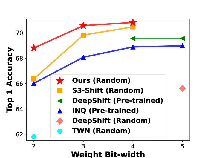
Figure 1: Benchmark low-bit DenseShift networks over SOTA low-bit Shift networks on ImageNet using the ResNet-18 model architecture.

Deep neural networks have demonstrated superior performance in diverse applications such as image classification, object detection, and image segmentation [17, 27, 6], and speech [29]. However, despite the high accuracy of multiplication-based deep neural networks, their computing resource requirement makes their deployment challenging, especially on low-resource devices. Recent research has explored multiplication-free neural networks that reduce memory footprint and overall energy consumption to address this issue.

Existing works on multiplication-free neural networks include binary [8], and ternary quantization [21]. They respectively constrain their weights in the range of $\{\pm 1\}$ and $\{0\}\cup\{\pm 1\}$, in order to replace multiplication computations with less expensive operations such as a sign flip operator. These low-bit quantization techniques make it possible to deploy deep learning models on resource-constrained edge devices. Moreover, [44] trades the multiplication operation with the addition operation, and [12, 22, 36] use the bit-shift operator to build power-of-two (PoT) quantized networks, known as Shift networks. Shift networks built upon a ternary base have a weight space of $\{0\}\cup\{\pm 2^{p}\}$. This means that multiplication operations can be replaced with bit-wise shift operations, which have highly efficient hardware implementations. In fact, [36] showed that with 4-bit weights and 8-bit activations, the shift-based MAC unit designed for Shift networks outperformed its counterpart for traditional uniform quantization by $2.4\times$ energy saving and 20% chip area saving using Samsung 5nm.

A recent study [22] proposes a weight reparameterization scheme $S^{3}$ for Shift network training, which significantly improves the accuracy of the ImageNet classification task under sub-4bits weight and does not require full-precision pre-training. However, $S^{3}$ has the following shortcomings: i) Existing Shift networks, including $S^{3}$, only support quantized activations during inference, limiting their performance gains and usefulness in various scenarios; ii) $S^{3}$ is only benchmarked on image classification and exhibits significant performance degradation under 2-bit weight; iii) Transfer learning tasks are unexplored.

In this study, we identify and address design limitations in current low-bit Shift networks through a detailed analysis, resulting in the proposal of DenseShift network. Our novel designs significantly enhance model capacity, inference efficiency, and transferability. The contributions of this study are outlined below.

First, our analysis reveals that zero weights in low-bit Shift networks reduce model capacity under limited bit widths. To address this issue, we propose a zero-free shifting mechanism that removes zero values from the weight space. This design enhances model representation capacity and improves performance under low-bit conditions, surpassing existing low-bit Shift networks.

Second, we introduce a novel inference approach for DenseShift networks that supports both floating-point and quantized activations. Our approach accelerates the dot-product computation by $1.6\times$ on ARMv8 CPU under FP16. Notably, DenseShift is the first Shift network that enables inference with non-quantized floating-point activations and the first to demonstrate performance improvement without relying on dedicated hardware such as ASIC or FPGA.

Third, we propose an efficient training algorithm for DenseShift networks adapted from the weight re-parameterization techniques [22]. Our sign-scale decomposition method breaks down the discrete weights into a binary sign term and a power-of-two scale term, and recursively re-parameterizes the exponent of the scale term as a combination of binary variables. This enables us to train low-bit DenseShift networks from a random initialization, achieving performance that is comparable to full-precision networks.

Fourth, while prior research works suffer from severe performance degradation when transferred to a new task, we propose a low-variance random initialization strategy to improve the model’s performance in transfer learning scenarios. We demonstrate that the weight values tend to gather towards the original point of the re-parameterization space during the initial stage of training, and as a result, a greater gradient signal is needed to push them to pass the threshold when the weights are randomly initialized with a large variance. By reducing the variance of weight initialization, the DenseShift network can be easily adapted to different tasks while maintaining competitive performance.

We conducted extensive experiments to evaluate the performance of our DenseShift network compared to various baselines on a diverse set of tasks across different fields. The results show that our proposed DenseShift network outperforms the state-of-the-art Shift network on the ImageNet classification task and achieves comparable performance to full-precision networks while having higher inference computational efficiency. As summarized in Fig. 1, DenseShift network performs significantly better in low-bit settings, especially under 2-bit condition. Specifically, our 2-bit and 3-bit quantized ResNet-18 on the classification task achieve $68.90\%$ and $70.57\%$ Top-1 accuracy respectively. Moreover, we demonstrate that our low-bit DenseShift networks can achieve full-precision performance in transfer learning scenarios across different domains, including computer vision and speech tasks. This study is the first to demonstrate this capability, to the best of our knowledge.

2 Related Works

Different approaches have been suggested to replace the expensive multiplication operation to mitigate the computational complexity of neural networks. Low-bit neural networks with binary weights [8, 39] or ternary weights [21] are examples of multiplication-free networks. While computationally inexpensive, their major flaw lies in the accuracy gap compared to their full-precision counterparts, as they suffer from under-fitting on large datasets. There are also works that utilize computationally cheaper operations, such as addition operations [5, 44, 46], square operations [35], or bit-shift operations [49, 14, 12, 31]. Compared to using binary or ternary weights, these methods achieve a low accuracy drop on large datasets but require higher weight representation bit-width as a trade-off. Some other works try to improve the performance of multiplication-free neural networks by using both addition and bit-shift operations [47], a sum of binary bases [25, 48], or sum of shift kernels [23], however, they remain computational costly as more operations are used per kernel.

In order to improve the accuracy of Shit networks under low-bit, [49] propose to fine-tune the pre-trained full-precision weights with a power-of-two quantizer in a group-by-group manner. [12] proposed a power-of-two quantizer design which allows training Shift networks from scratch. However, initialization with a pre-trained full-precision checkpoint is still critical for achieving high accuracy under low-bit. [22] proposes a weight reparameterization technique $S^{3}$ for training low-bit Shift networks. It points out the design flaw of the weight quantizer for low-bit Shift networks and proposes to decompose a discrete parameter in a sign-sparse-shift 3-fold manner to improve ImageNet classification accuracy under sub-4bits conditions significantly and no longer rely on full-precision pre-training.

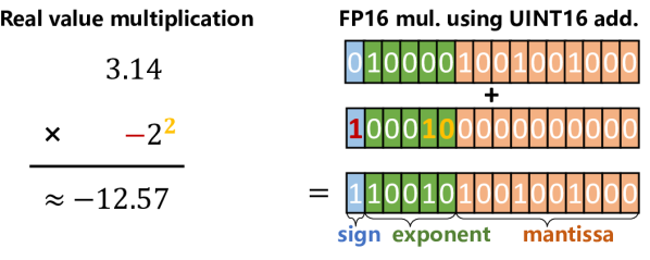
Figure 2: The multiplication between a float number and a positive or negative power-of-two integer can be implemented by an integer addition instruction, which allows DenseShift networks inference on most existing hardware efficiently. The FP16 dot-product computation achieved $1.6\times$ speed up on ARM A57 CPU using this technique as discussed in Sec. 3.1.1.

3 DenseShift Network

The following section introduces the proposed DenseShift network, highlighting the benefits for inference deployment, and providing a detailed analysis of weight encoding space, training mechanisms and weight initialization strategies employed.

3.1 DenseShift with Zero-Free Shifting

Typical Shift networks use a weight space with $n$-bits to encode weight values, allowing up to $2^{n}$ discrete values. However, since the values are usually centred around zero, the utilization rate of the encoding space is reduced when zero is included. This becomes significant under low-bit conditions, particularly when $n\leq 4$.

Taking $n=2$ bits as an example, the weight space allows for $4$ discrete weight values to be encoded. In a typical Shift network, these would include $w=\{-1,0,+1\}$, ignoring the potential for adding a fourth weight value. In DenseShift however, as there is no zero-value, we can now encode weight values of $w=\{-2,-1,+1,+2\}$ with the same number of bits. This increases the overall range of weight values supported, allowing DenseShift to significantly outperform existing Shift networks, especially under low-bit weight conditions as summarized in Fig. 1.

3.1.1 Inference with floating-point activation

The Zero-Free Shifting design also brings additional benefits to inference. To the best of our knowledge, all existing Shift networks rely on using quantized activations in order to effectively replace the multiplication between the power-of-two weights and activations with bit-shift instructions. However, there are some challenges with quantized activations when applied in practice. For instance, in LSTM and Transformer models, many operators, such as softmax or addition, are unable to compute directly with the quantized activations. Instead, it must first dequantize in order to compute, then re-quantize the results, which leads to extra inference latency. This is also seen with large language models (LLM) as shown in [10] where 8-bit quantization could not maintain full-precision performance on LLMs with models that exceeded 6.7 billion parameters because the fixed-point quantization can not handle activations with a large dynamic range well, leading to a significant accuracy degradation of the LLMs. These issues above impair the performance gains or usability of the existing power-of-two quantization methods.

In this work, we propose a method to calculate the multiplication between a floating-point number and positive or negative power-of-two numbers using integer addition instructions. Our approach allows DenseShift networks to perform inference directly on non-quantized floating point activations, thus avoiding the above issues.

In the following section, we describe how to achieve equivalent multiplication between floating-point numbers and power-of-two numbers using lower-bit integer addition. A floating-point number is obtained by Eq. 1.

$${\sf{fl}}(x)=(-1)^{x_{\textbf{s}}}\times 2^{x_{\textbf{e}}+\textbf{e}_{\textbf{bias}}}\times(1+\frac{x_{\textbf{m}}}{2^{\textbf{m}_{\textbf{bits}}}-1}),$$ (1)

Where ${\sf{fl}}(\cdot)$ is the float representation, $x_{\textbf{s}}$ is the sign bit value, $x_{\textbf{e}}$ is the unsigned integer value represented by the exponent bits, $x_{\textbf{m}}$ is the unsigned integer value represented by the mantissa bits, and $\textbf{m}_{\textbf{bits}}$ is the mantissa bit-width and $\textbf{e}_{\textbf{bias}}$ the constant exponent bias value defined in the floating-point standard. For the 32-bit float format defined in the IEEE 754 standard, $\textbf{m}_{\textbf{bits}}=23$ and $\textbf{e}_{\textbf{bias}}=-127$.

From the floating-point representation, it is clear that the multiplication of a floating-point value with a power-of-two number is equivalent to adding a corresponding integer to the exponent bit of the floating-point number. The negation of a floating-point number is equivalent to performing a bit-flip on the sign bit, which can be achieved by adding one to the sign bit. Therefore, the multiplication of a float number with a positive or a negative power-of-two number can be performed by one single lower-bit integer addition operation on its sign and exponent bits as described in Fig. 2. As an example, the multiplication between a 32-bit float number and a positive or negative power-of-two integer can be implemented with a 9-bit integer adder on its sign bit and exponent bits. Related works [19, 40] show that replacing floating-point multiplication with fixed point addition can save $37\times$ energy cost and $56\times$ chip area cost at 32-bit, and using an 8-bit integer adder can further reduce $3.3\times$ energy cost and $3.8\times$ chip area. This highlights the potential of DenseShift networks to reduce power consumption and chip area for AI chips.

Furthermore, our proposed DenseShift inference approach is compatible with the existing hardware. Thanks to its Zero-Free Shifting design, the multiplication instruction in the DenseShift inference can be replaced by one single integer addition instruction which requires fewer execution cycles in general as described in Eq. 2 and Fig. 2.

$${\sf{fl}}(2^{p}x)={\sf{Add}_{\sf{uint}}}({\sf{fl}}(x),{\sf{fl}}(2^{p+\textbf{e}_{\textbf{bias}}}))$$ (2)

Where ${\sf{fl}}(\cdot)$ is the float representation, $\textbf{e}_{\textbf{bias}}$ the constant exponent bias value defined in the floating-point standard. ${\sf{Add}_{\sf{uint}}}(\cdot,\cdot)$ is the integer addition.

Unlike the UINT8 and UINT16 formats, widely supported by existing hardware, the FP8 and FP16 formats have relatively limited hardware support. This is because floating-point numbers have the disadvantage of significant calculation error under lower bits, which can not satisfy the needs of many computing tasks. As a result, most existing hardware do not support low-precision floating-point arithmetic. They are reserved for data storage or only supported by limited operators. For instance, ARMv8 and X86 AVX2 instruction sets do not support FP16 arithmetic. When an operation is required, it is necessary to convert the FP16 to FP32 in registers before the operation and convert it back afterward. The same strategy is used by NVIDIA GPUs while processing FP8 [34]. On this hardware, we can use the corresponding unsigned int addition to replace the floating-point multiplication instruction, which has the potential to achieve inference speed up. It’s important to note that our proposed approach is not applicable to zero-multiplication, as it necessitates additional operations for implementation, making it less efficient on general hardware. This underscores the advantages of our zero-free shifting design.

As a proof-of-concept, we implement DenseShift using this technique and compare it to floating-point dot-product using a vectorized software implementation. Both weights and activations are provided to the compute kernel as FP16. The DenseShift kernel performs bit-wise manipulation and adds the sign and exponents of the weight and activation values together (see Fig. 2), effectively replacing the floating-point multiplication with a simple integer addition. The result of this integer addition is then cast back to FP32 for accumulation. This implementation is compared to the dot-product baseline adapted from the FP16 GEMM kernel of the open-source inference library NCNN [33] for the ARMv8 hardware. All experiments were run on ARM A57 CPU using NEON SIMD architecture and count the average time consumption. We run experiments for 4096 data points. The results averaged over 1000 runs show that the latency for the floating-point dot-product and our proposed technique are $5.98\mu s$ and $3.76\mu s$, respectively. In other words, DenseShift kernel using the proposed floating-point technique obtains 1.6× speed-up.

Our DenseShift implementation can be further optimized to reduce overall memory consumption requirements; since the weight values are constrained to power-of-two numbers, their mantissa will always be zero and thus are not needed in the compute kernel. Instead, only the weight’s sign and exponent are sent to the compute kernel, requiring only 7 bits, and can be represented with a single unsigned 8-bit integer. In addition, our proposed approach has the potential to be extended to other neural network layers beyond matrix multiplication for efficient computation.

3.1.2 Inference with quantized activation

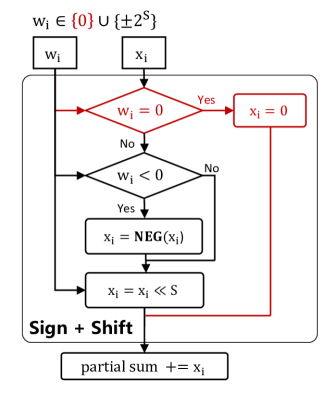
(a) Shift MAC kernel

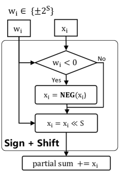
(b) DenseShift MAC kernel

Figure 3: Compare the Multiply-Accumulate (MAC) operations in Shift and DenseShift for quantized activation. The DenseShift MAC is more efficient as its $w_{i}$ excludes zero.

With a zero-free weight space design, DenseShift simplifies the inference computation on fixed-point quantized activations as well. Figure 3 compares the Multiply-Accumulate (MAC) operation between DenseShift and Shift networks. The Shift network MAC kernel requires special handling when $w_{i}=0$, as shown in Fig. 3(a), which bypasses sign-flip and bit-shift operations and pass a value of $x_{i}=0$ to the accumulator instead. Since DenseShift guarantees that $w_{i}$ will never be zero, this branch is no longer required, as shown in Fig. 3(b). Therefore, the inference computation in DenseShift networks is simpler and more efficient than in existing Shift networks. A NEON SIMD dot-product kernel was developed on an ARM A57 CPU to demonstrate DenseShift ’s computational efficiency over existing Shift networks. The experiments were performed with INT8 for 4096 data points, and the results showed that DenseShift kernel had a $1.48\times$ speed-up compared to a Shift kernel implementation, with the latency of $1.79\mu s$ and $2.65\mu s$, respectively.

Aside from experimental demonstration, we also theoretically show that removing zeros from the weight space doesn’t affect the representation power of DenseShift models, see the Supplementary Material. Thoerem 1 confirms that there is a DenseShift network that can reach to the same accuracy as any Shift network if properly trained. Theorem 2 shows there is a DenseShift network that can attain the same capacity compared with a full-precision network.

3.2 Sign-Scale Decomposition for Efficient Training

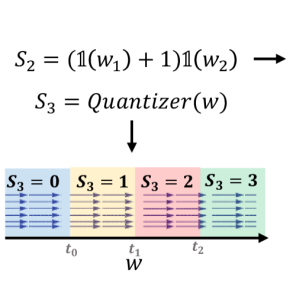
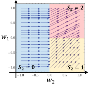
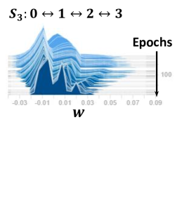
Figure 4: Top Left: The optimization space of the shifting parameter $S_{3}$ defined by the sign-shift quantizer adapted from [12]. The arrow direction represents the moving direction of the continuous weight $w$ in the optimization space when the gradient update of the shifting parameter $S_{T}$ is positive. Bottom Left: The actual continuous weight histogram variation of $S_{3}$ defined by the 3-bit sign-shift quantizer during training. Top Right: The phase plane of the re-parameterization space of $S_{2}$ defined by a recursive product of binary variables ($\frac{\partial w_{2}}{\partial t}=\mathbbm{1}(w_{1})+1,\frac{\partial w_{1}}{\partial t}=\mathbbm{1}(w_{2})$). Bottom Right: Some sampled actual weight traces of $S_{2}$ on the optimization space defined by a recursive product of binary variables during training. The weight trajectories show that the $S_{2}$ values can quickly move among multiple discrete values during training and are no longer limited to the two adjacent values of the quantizer’s thresholds.

This section discuss the training algorithm for DenseShift and how to achieve a performance comparable to its full-precision counterpart. We propose to use sign-scale decomposition inspired by [22] which design for Shift networks with zero weights. Our training method decomposes the discrete weights of DenseShift networks into two parts: a binary base term $w_{\mathrm{sign}}$ and a PoT scale term which shifts the input activation for $S$ bits:

$$w_{\mathrm{shift}}=\underbrace{\{2\mathbbm{1}(w_{\mathrm{sign}})-1\}}_{\mathclap{\text{Sign}}}\overbrace{2^{S_{T}}}^{\mathclap{\text{Scale}}},$$ (3)

where $\mathbbm{1}(\cdot)$ is the Heaviside function mapping all positive values to one and the remaining to zero.

Next, we recursively re-parameterize the shifting parameter $S$ as a combination of $t$ binary variables to address the weight freezing problem:

$$S_{0}=0,\ S_{t}=\mathbbm{1}(w_{t})(S_{t-1}+1),\quad\quad 1\leq t\leq T.$$ (4)

In the following, we demonstrate the re-parameterization on positive $S$ values using $3$-bit case as an example, and the negative $S$ values can be obtained by adding a constant bias term. We define a 3-bit DenseShift network with discrete weights $w_{\mathrm{shift}}\in\{\pm 1,\pm 2,\pm 4,\pm 8\}$. This network can be re-parameterized as:

$$S_{3} = \mathbbm{1}(w_{3})\{\mathbbm{1}(w_{2})\{\mathbbm{1}(w_{1})+1\}+1\},$$ (5)

$$w_{\mathrm{shift}} = \{2\mathbbm{1}(w_{\mathrm{sign}})-1\}2^{S_{3}}.$$ (6)

Note that all the weights $\{w_{\mathrm{sign}},w_{1},w_{2},w_{3}\}$ are trained in full-precision. By representing the original shift parameter $S_{3}$ with three full-precision parameters $w_{1}$, $w_{2}$, and $w_{3}$, we are projecting the optimization process from 1D space to higher-dimensional 3D space, making the shift parameter easier to vary between different scales and thus easier to learn. Compared to [22], our approach eliminates the dense weight regularizer. This not only removes the need to tune an additional hyper-parameter but also simplifies the usage of our algorithm. While such training requires $(N+1)$ floating-point references, it is not as memory expensive as it appears, especially under 2/3-bit weight conditions. The memory is dominated by the activation with a large batch size during training.

To better understand the advantages of our weight reparameterization approach over the quantizer-based training method, in Fig. 4, we visualize the optimization spaces of the shifting parameter $S$ defined i) by a quantizer (figure left part) and ii) by a recursive product of binary variables (figure right part). In the quantizer’s optimization space, the continuous weights accumulate at the three discontinuities of the quantizer as discussed in several earlier works [32, 26, 22]. This observation implies that the weights attracted by the discontinuities could not move freely on the optimization space during training. In contrast, the weights in the optimization space defined by the recursive product of binary variables are gathered at the origin of the optimization space, and the value of the shifting parameter $S$ can vary easily according to the gradient update signal. The visualization shows our re-parameterization promotes the shifting parameters $S$ to oscillate in an extensive range value during training instead of oscillating around the quantizer’s threshold values. This design reduces the optimization space’s rigidness and allowing the model to converge to a better solution [22].

The local learning rate of individual parameter $w_{\mathrm{sign}}$ in the proposed training scheme is significantly larger than the global learning rate on the discrete weight $w_{\mathrm{shift}}$. Furthermore, we analyze the backward gradient computation of our proposed decomposition. We estimate the backward gradient across the Heaviside function using a Straight-Through-Estimator (STE) [3]. The gradient update towards $w_{\mathrm{sign}}$ is calculated as:

$$\frac{\partial\text{Loss}}{\partial w_{\mathrm{sign}}}=\frac{\partial\text{Loss}}{\partial w_{\mathrm{shift}}}{2^{S_{T}}},$$ (7)

where $2^{S_{T}}\in\{1,2,...,2^{T}\}.$ From Eq. 7 we observe that $2^{S_{T}}$ plays a role of learning rate scale factor, and it has an extensive value range. Hence, it may significantly impact the gradient update scale. Based on our observation, we propose a local learning rate re-scaling strategy to address this issue. We replace Eq. 7 with Eq. 8 during backward propagation to re-scale local gradient updates:

$$\frac{\partial\text{Loss}}{\partial w_{\mathrm{sign}}}=\frac{\partial\text{Loss}}{\partial w_{\mathrm{shift}}}{\sqrt{{S_{T}+1}}}.$$ (8)

ImageNet experiments indicates that the local learning rate re-scaling enhances the accuracy of 2bit and 3bit ResNet-18 models by 0.3% and 0.7%, respectively.

3.3 Low-Variance Random Initialization for Transfer Learning

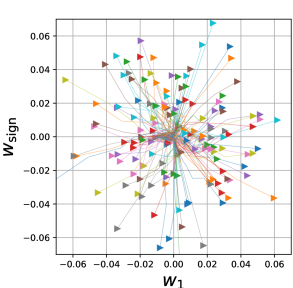
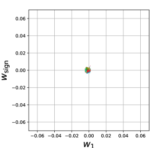
Figure 5: Re-parameterized weight trace visualization of a 2-bit DenseShift ResNet-18 trained on ImageNet dataset, the “triangle” indicates the initial point. These visualizations motivate us to develop low-variance initialization. Left panel: Kaiming initialization. Right panel: Low-variance initialization.

We encountered difficulties when applying the above method in the transfer learning scenario. Most transfer learning tasks follow the following training paradigm: i) Pre-train a backbone model on a large dataset; ii) Remove and add new layers to the backbone model and randomly initialize the new layer; iii) Finetune the new model on a downstream task. During our experiments, we noticed that when we finetune a pre-trained DenseShift backbone with randomly-initialized DenseShift layers in an end-to-end manner, the model suffers from severe performance degradation or loss divergence. Such performance degradation also exists for existing Shift networks.

We analyzed the difference between the pre-trained weights and the randomly-initialized weights in the DenseShift model and noticed that the variance of the former is much lower than that of the latter. To better understand this phenomenon, we trained a 2-bit DenseShift network and noticed that when using the default Kaiming initialization [15], the weight values tend to gather towards the origin point of the re-parameterization space during the first few training epochs, as shown in figure 5. This indicates that the initialized weight values are too far from the centre, an unwanted behaviour. More precisely, the weight values are far from the thresholds, meaning a greater initial gradient signal is needed to push them to pass the thresholds. In the transfer learning scenario, the backbone weight values are easier to change than the new Kaiming initialized layers. In fact, we argue that it is precisely this behavior that damages the pre-trained backbone during transfer learning.

To easily transfer a DenseShift network to other tasks, we suggest randomly initializing all re-parameterized variables with a small standard deviation. We name it low-variance random initialization. Specifically, we chose a standard deviation of $10^{-3}$ for all the experiments in this paper. The experiments in Sec. 4.2 demonstrate that our low-variance random initialization strategy is required for achieving competitive performance on transfer learning tasks such as object detection and semantic segmentation. As evident from Table 3, the SSD 300 model shows a decrease in mAP without low-variance random initialization. Moreover, the FCOS object detection experiments, detailed in Table 4, which employ quantized feature-pyramid networks, demonstrate instability and fail to converge during training without our proposed initialization. In this paper, all DenseShift experiments use this initialization uniformly since we do not observed any negative impact on the model performance when training from scratch with our proposed initialization.

ResNet-18
Kernel	Methods	W Bits	Init.	Top-1 (%)
Multi.	FP32	32	R	69.6
	TTQ [51]	2	PT	66.6
Sum of Sign Flips	Lq-Nets [48]	2	R	68.0
	Lq-Nets [48]	3	R	69.3
	Lq-Nets [48]	4	R	70.0
Sign Flip	BWN [39]	1	R	60.8
	HWGQ [4]	1	R	61.3
	BWHN [20]	1	R	64.3
	IR-net [38]	1	R	66.5
	TWN [21]	2	R	61.8
	LR-net [41]	2	R	63.5
	SQ-TWN [11]	2	R	63.8
	INQ [49]	2	PT	66.02
	S3 -Shift [22]	2	R	66.37
Shift + Sign Flip	Ours	2	LVR	68.90
	INQ [49]	3	PT	68.08
	INQ [49]	4	PT	68.89
	INQ [49]	5	PT	68.98
	DeepShift [12]	5	R	65.63
	DeepShift [12]	4	PT	69.56
	DeepShift [12]	5	PT	69.56
	S3 -Shift [22]	3	R	69.82
	Ours	3	LVR	70.62
	STE [37]	4	PT	69.98
	S3 -Shift [22]	4	R	70.47
	Ours	4	LVR	70.94

Table 1: Comparison of SOTA methods using DenseShift ResNet-18 trained on ImageNet. Initialization defined as: R is Kaiming Normal Random initialization, PT is initialization with a Pre-Trained full-precision network, and LVR is our Low-Variance Random initialization.

ResNet-50
Kernel	Methods	W Bits	Init.	Top-1 (%)
Multi.	FP32	32	R	76.00
Sum of Sign Flips	Lq-Nets [48]	2	R	75.10
	Lq-Nets [48]	4	R	76.40
Shift + Sign Flip	INQ [49]	5	PT	74.81
	DeepShift [12]	6	PT	75.29
	S3 -Shift [22]	3	R	75.75
	STE [37]	4	PT	76.40
	Ours	2	LVR	75.62
	Ours	3	LVR	76.55
	Ours	4	LVR	76.53
ResNet-101
Kernel	Methods	W Bits	Init.	Top-1 (%)
Multi.	FP32	32	R	77.37
Shift + Sign Flip	Ours	2	LVR	77.45
	Ours	3	LVR	77.93
	Ours	4	LVR	77.96

Table 2: Comparison of SOTA methods using DenseShift ResNet-50/101 trained on ImageNet.

4 Experiments

4.1 ImageNet Classification

Model and Dataset: We benchmark our proposed method with different bit-widths. To verify the effectiveness and robustness, we apply DenseShift to ResNet-18/50/101 architectures and evaluate on ILSVRC2012 dataset [9] with data augmentation and pre-processing strategy proposed in [16] and training strategy from [22]. Following [39, 28, 48], all but the first convolution layers are quantized.
Experiment Results: Results are shown in Table 1 and 2. We compare our proposed method with SOTA low-bit multiplication-free networks using binary weights [39, 4, 20, 38], ternary weights [21, 41, 11], PoT weights [49, 12, 22] and more complex kernel [48]. We observe that DenseShift achieves SOTA performance on multiple network architectures and significantly outperforms the baseline with higher computational complexity.

Methods	Quantized		LVR	W Bits	mAP
	Back	Head	Init
FP32	$-$	$-$	$-$	32	26.00
Ours		$-$	$-$	3	26.23
				3	25.75
			$-$	3	24.21

Table 3: DenseShift performs well on object detection. It confirms our low-variance initialization is necessary to keep high accuracy. We use DenseShift SSD300 v1.1 with ResNet-50 backbone finetuned on COCO object detection task. Back is the backbone neural architecture, Head is the detection head. Check-mark represents performing DenseShift quantization.

Methods	Quantized			W Bits	mAP
	Back	FPN	Head
FP32	$-$	$-$	$-$	32	39.0
Ours		$-$	$-$	2	39.3
			$-$		38.7
					37.1
		$-$	$-$	3	39.6
			$-$		39.3
					37.7
		$-$	$-$	4	39.8
			$-$		39.6
					38.1

Table 4: DenseShift FCOS with ResNet-50 backbone finetuned on COCO object detection task.

4.2 Transfer Learning

Model and Dataset: We use TorchVision implementation to verify the effectiveness and robustness of our proposed algorithm on transfer learning tasks. For object detection, we benchmark our proposed method on the bounding box detection track of MS COCO [24]. As proof of concept, we use SSD300 v1.1 [27] with the obsolete VGG backbone replaced with ResNet-50 backbone. To demonstrate competitive performance, we use FCOS [43] with ResNet-50 backbone. For semantic segmentation, we benchmark our proposed method on a subset of MS COCO containing the 20 categories of Pascal VOC [13]. We use DeepLab V3 [6] with ResNet-50 backbone architecture. The DenseShift ResNet-50 backbone is trained from the previous section and we compare against full-precision baselines using the same training strategy.
Experiment Results: Tables 3 and 4 illustrate that our 3-bit SSD300 and FCOS achieve similar performance to their full-precision counterparts. Table 5 illustrate that our 3-bit DeepLab surpasses its full-precision counterpart.

Methods	Quantized		W Bits	mIoU	Global
	Back	Head			Correct
FP32	$-$	$-$	32	66.4	92.4
Ours		$-$	2	65.8	92.2
				66.1	92.4
		$-$	3	68.0	92.6
				67.4	92.8
		$-$	4	66.0	92.3
				66.3	92.0

Table 5: DenseShift DeepLab V3 with ResNet-50 backbone finetuned on COCO semantic segmentation task.

4.3 Speech Task

Model and Datasets: To further demonstrate the generalization of DenseShift networks, we experiment on an end-to-end spoken language (E2E SLU) task with ResNet-18 architecture. We benchmark our method on the Fluent Speech Commands (FSC) dataset. The FSC dataset [29] comprised single-channel audio clips collected using crowd sourcing. Participants were requested to speak random phrases for each intent twice. The dataset contained 30,043 utterances spoken by 97 different speakers, each utterance contains three slots: action, object, and location. We considered a single intent as the combination of all the slots (action, object and location), resulting 31 intents in total.
Experiment Results: Results in Table 6 are benchmarked against full-precision and SOTA Shift networks performance. Our results demonstrates that our method can be applied to a field unrelated to the original CV field and can surpass full-precision performance as well.

Method	W Bits	Val	Test
[30]	32	89.50	98.80
[2]	2	90.66	98.41
	3	90.31	98.41
Ours	2	90.73	98.60
	3	90.70	98.58

Table 6: DenseShift ResNet-18 architecture on End-to-End Spoken Language Understanding

4.4 Quantized Activation

Considering that Shift networks require fixed-point activation to achieve computational efficiency, we provide quantized activation experiments to verify the feasibility and find that 4-bit activation can maintain competitive performance on most CV tasks with PACT quantization [7]. Results shown in Tables 7, 8 and 9 demonstrate that DenseShift can attain similar performance to their full-precision counterparts. Hence, we believe DenseShift networks generalize well and are independent of other layers.

Network	A Bits	Top-1 Acc (%)
Architecture		2 Bit	3 Bit	4 Bit
ResNet-18	32	68.90	70.62	70.94
	8	68.86	70.46	70.95
	4	68.56	70.00	70.35
ResNet-50	32	75.62	76.55	76.53
	4	75.27	76.18	76.63

Table 7: Quantized activation experiments using DenseShift ResNet architectures on ImageNet classification task. A-Bits defined as activation bitwidth.

Quantized			A Bits	mAP
Back	FPN	Head		3 Bit	4 Bit
		$-$	32	39.3	39.6
		$-$	4	39.6	39.6
			32	37.7	38.1
			4	37.8	37.8

Table 8: Quantized activation experiments using DenseShift FCOS with ResNet-50 backbone finetuned on COCO object detection task.

Quantized		A Bits	mIoU
Back	Head		2 Bit	3 Bit
	$-$	32	65.8	68.0
	$-$	4	64.9	66.3
		32	65.5	66.4
		4	65.2	65.9

Table 9: Quantized activation experiments using DenseShift DeepLab V3 with ResNet-50 backbone finetuned on COCO semantic segmentation task.

4.5 Ablation Study

Training epochs. As highlighted in prior studies [1, 8, 42, 22, 45], the training of binary variables necessitates additional epochs due to the instability arising from frequent sign variations. Our experiments in Table 10 verified the impact of training epochs on the network performance for the re-parameterized training of DenseShift networks. Apart from the number of epochs, all other model settings and training strategies adhere to Sec. 4.1.

Network	W Bits	Training Epochs
Architecture		90	150	200
ResNet-18	2	67.36	68.41	68.90
	3	69.30	69.91	70.62

Table 10: Ablation study on training epochs using DenseShift ResNet-18 architectures on ImageNet classification task.

5 Conclusion

We present DenseShift with zero-free shifting and sign-scale decomposition for constructing high-performance low-bit Shift networks with high training and inference efficiency. For the first time, Shift networks support inference with non-quantized floating-point activations and achieve performance gain on general hardware such as ARM CPU. Furthermore, we propose a low-variance random initialization strategy that enhances the performance of DenseShift networks in transfer learning, allowing the networks to adapt to various tasks without significant performance degradation. Our extensive experiments on various tasks demonstrate that DenseShift networks outperform current state-of-the-art Shift networks in classification tasks and achieve comparable performance to full-precision models in object detection and semantic segmentation tasks. This breakthrough represents a significant advancement for low-bit Shift networks.

Appendix A Proof of Theorems

Theorem 1.

Suppose a shift neural network in the form $\hat{f}_{\mathbf{w}}(\mathbf{x})=\sum_{j=1}^{J}\sum_{k=1}^{d_{j}}w^{j}_{k}h^{j}_{k}(\mathbf{x}),$ where $w^{j}_{k}\in\{0\}\cup\{\pm 2^{p}\}$ approximates the true unknown function $f(\mathbf{x}),\mathbf{x}\in{\rm I\!R}^{d}.$ There is another dense neural network with $w^{\prime j}_{k}\in\{\pm 2^{p}\}$ that has a similar form $\hat{f}_{\mathbf{w}^{\prime}}(\mathbf{x})=\sum_{j=1}^{J}\sum_{k=1}^{d^{\prime}_{j}}\mathbf{w}^{\prime j}_{k}h^{\prime j}_{k}(\mathbf{x})$, such that $\forall\mathbf{x}\in{\rm I\!R}^{d},\hat{f}_{\mathbf{w}}(\mathbf{x})=\hat{f}_{\mathbf{w}^{\prime}}(\mathbf{x}).$

Proof.

The proof is straightforward by isolating zero shifts, and recreating these null weights in a larger dense shift network with opposite weight signs. Define the $j^{\text{th}}$ layer as

$$h^{j}(\mathbf{x})=a(\mathbf{W}^{j}h^{j-1}(\mathbf{x})+\mathbf{b}^{j}),$$

where $h^{0}(\mathbf{x})=\mathbf{x}$, $J$ is the total number of layers each of output dimension $d_{j}$ and $\mathbf{W}$ of size $d_{j}\times d_{j-1}$ can be a Toeplitz matrix for a convolutional layer, $a(\cdot)$ is the activation function, and $\mathbf{b}$ is the bias term. Define the shift network approximation of $f(\mathbf{x})$ as

$$\hat{f}_{\mathbf{w}}(\mathbf{x})=\sum_{j=1}^{J}\sum_{k=1}^{d_{j}}w^{j}_{k}h^{j}_{k}(\mathbf{x})$$

in which $w^{j}_{k}\in\{0\}\cup\{\pm 2^{p}\}$ defines a shift network. We re-create an equivalent desne shift network by isolating null weights $w^{j}_{k}=0$ and replacing them with a larger dense shift network of an arbitrary weights but with opposite signs. Now suppose $\mathbf{w}_{0}=\{k\mid w^{j}_{k}=0\}$ and $\mathbf{w}_{1}=\{k\mid w^{j}_{k}\neq 0\}$ where $\mathbf{w}=[\mathbf{w}_{0}^{\top}\mathbf{w}_{1}^{\top}]$, $d_{j}=d_{0j}+d_{1j}$

$$\hat{f}_{\mathbf{w}}(\mathbf{x})=\sum_{j=1}^{J}\left[\sum_{k=1}^{d_{0j}}w^{j}_{0k}h^{j}_{0k}(\mathbf{x})+\sum_{k=1}^{d_{1j}}w^{j}_{1k}h^{j}_{1k}(\mathbf{x})\right].$$

Assume $\tilde{\mathbf{w}}\in\{\pm 2^{p}\}$ is a nonzero shift arbitrary vector of elements $\tilde{w}_{0k}$,

$$\sum_{j=1}^{J}\left[\sum_{k=1}^{d_{0j}}\mathbf{w}^{j}_{0k}h^{j}_{0k}(\mathbf{x})+\sum_{k=1}^{d_{1j}}\mathbf{w}_{1k}h^{j}_{1k}(\mathbf{x})\right]$$

$$= \sum_{j=1}^{J}\left[\sum_{k=1}^{d_{0j}}\tilde{\mathbf{w}}^{j}_{k}h^{j}_{0k}(\mathbf{x})-\tilde{\mathbf{w}}^{j}_{k}h^{j}_{0k}(\mathbf{x})+\sum_{k=1}^{d_{1j}}\mathbf{w}_{1k}h^{j}_{1k}(\mathbf{x})\right].$$

By defining $\mathbf{w}^{\prime}=[\tilde{\mathbf{w}},-\tilde{\mathbf{w}},\mathbf{w}_{0}]$ of increased size $d^{\prime}_{j}={d_{0j}+d_{j}\geq d_{j}}$, one may rearrange terms and rewrite the neural approximate as

$$\hat{f}_{\mathbf{w}^{\prime}}(\mathbf{x})=\sum_{j=1}^{J}\sum_{k=1}^{d^{\prime}_{j}}\mathbf{w}^{\prime j}_{k}h^{\prime j}_{k}(\mathbf{x}),$$

where $h^{\prime j}_{k}$ is either $h^{j}_{0k}$ or $h^{j}_{1k}$ depending on the dense shift weight $\mathbf{w}^{\prime j}_{k}\in\{\pm 2^{p}\}$. ∎

Theorem 2.

Dense shift network with a Lischitz activation function is a universal approximator on a compact set $K$ for any measurable continuous function $f\in C(K)$ with respect to the measure $\mu$, given that its weight and activations $\mathbf{w},h(\mathbf{x})$ remain close to the regular network in the following sense

$$\int_{K}\left(\sum_{j=1}^{J}\sum_{k=1}^{d_{j}}\left(\mathbf{w}^{j}_{k}h^{j}_{k}(\mathbf{x})-\mathbf{w}^{\prime j}_{k}h^{\prime j}_{k}(\mathbf{x})\right)\right)^{2}d\mu<{\epsilon\over 4},$$

where $\epsilon\over 4$ is the approximation quality of the regular neural network, $\left(\mathbf{w},h^{j}(\mathbf{x})\right)$ and $\left(\mathbf{w}^{\prime},h^{\prime j}(\mathbf{x})\right)$ are the weight and activations of the regular and DenseShift networks in layer $j$, respectively.

Proof.

It is well-known that shallow networks are universal approximator [18] as well as deep networks [50]. These results holds in infinity norm, so is also valid in $\ell_{p}$ norm with $p<\infty$. For the simplicity of the mathematical mechanics here we only focus on the multilayer perceptron [18] on $\ell_{2}$ norm

$$\left\lVert f-\hat{f}\right\rVert=\int_{K}\left|f(\mathbf{x})-\hat{f}(\mathbf{x})\right|^{2}d\mu$$ (9)

Suppose $\hat{f}_{\mathbf{w}}$ is a real weight neural network and $\hat{f}_{\mathbf{w}^{\prime}}$ is a dense shift version of the same network $\hat{f}_{\mathbf{w}}$, of course with weights $\mathbf{w}^{\prime}\in\{\pm 2^{p}\}$.

$$\left\lVert{f}-\hat{f}_{\mathbf{w}^{\prime}}\right\rVert$$ (10)

$$= \int_{K}\left|f(\mathbf{x})-\hat{f}_{\mathbf{w}^{\prime}}(\mathbf{x})\pm\hat{f}_{\mathbf{w}}(\mathbf{x})\right|^{2}d\mu$$

$$= \int_{K}|f(\mathbf{x})-\hat{f}_{\mathbf{w}}(\mathbf{x})|^{2}d\mu$$ (13)

$$+\int_{K}|\hat{f}_{\mathbf{w}}(\mathbf{x})-\hat{f}_{\mathbf{w}^{\prime}}(\mathbf{x})|^{2}d\mu$$

$$+2\int_{K}|[f(\mathbf{x})-\hat{f}_{\mathbf{w}}(\mathbf{x})][\hat{f}_{\mathbf{w}}(\mathbf{x})-\hat{f}_{\mathbf{w}^{\prime}}(\mathbf{x})]|d\mu.$$

In order to show that shift networks are universal approximator it is enough to show that $\left\lVert f-\hat{f}_{\mathbf{w}^{\prime}}\right\rVert$ is bounded by an arbitrarily small $\epsilon>0$. The first term (13) is bounded by $\epsilon\over 4$ [18]. The second term (13) is bounded given the shift net closeness assumption

$$\int_{K}|\hat{f}_{\mathbf{w}}(\mathbf{x})-\hat{f}_{\mathbf{w}^{\prime}}(\mathbf{x})|^{2}d\mu$$

$$= \int_{K}\left(\sum_{j=1}^{J}\sum_{k=1}^{d_{j}}\mathbf{w}^{j}_{k}h^{j}_{k}(\mathbf{x})-\sum_{j=1}^{J}\sum_{k=1}^{d_{j}}\mathbf{w}^{\prime j}_{k}h^{\prime j}_{k}(\mathbf{x})\right)^{2}d\mu$$

$$< {\epsilon\over 4}$$

The last term (13) is bounded by ${\epsilon\over 2}$ thanks to the Cauchy-Schwartz inequality. So (9) is bounded by $\epsilon$ by merging the pieces together. ∎

References

- [1] Milad Alizadeh, Javier Fernández-Marqués, Nicholas D Lane, and Yarin Gal. An empirical study of binary neural networks’ optimisation. In International Conference on Learning Representations, 2018.
- [2] Anderson R. Avila, Khalil Bibi, Rui Heng Yang, Xinlin Li, Chao Xing, and Xiao Chen. Low-bit shift network for end-to-end spoken language understanding, 2022.
- [3] Yoshua Bengio. Estimating or propagating gradients through stochastic neurons. CoRR, abs/1305.2982, 2013.
- [4] Zhaowei Cai, Xiaodong He, Jian Sun, and Nuno Vasconcelos. Deep learning with low precision by half-wave gaussian quantization. In Proceedings of the IEEE conference on computer vision and pattern recognition, pages 5918–5926, 2017.
- [5] Hanting Chen, Yunhe Wang, Chunjing Xu, Boxin Shi, Chao Xu, Qi Tian, and Chang Xu. Addernet: Do we really need multiplications in deep learning? In Proceedings of the IEEE/CVF Conference on Computer Vision and Pattern Recognition, pages 1468–1477, 2020.
- [6] Liang-Chieh Chen, George Papandreou, Florian Schroff, and Hartwig Adam. Rethinking atrous convolution for semantic image segmentation, 2017.
- [7] Jungwook Choi, Zhuo Wang, Swagath Venkataramani, Pierce I-Jen Chuang, Vijayalakshmi Srinivasan, and Kailash Gopalakrishnan. Pact: Parameterized clipping activation for quantized neural networks. arXiv preprint arXiv:1805.06085, 2018.
- [8] Matthieu Courbariaux, Yoshua Bengio, and Jean-Pierre David. Binaryconnect: Training deep neural networks with binary weights during propagations. In Advances in neural information processing systems, pages 3123–3131, 2015.
- [9] Jia Deng, Wei Dong, Richard Socher, Li-Jia Li, Kai Li, and Li Fei-Fei. Imagenet: A large-scale hierarchical image database. In 2009 IEEE conference on computer vision and pattern recognition, pages 248–255. Ieee, 2009.
- [10] Tim Dettmers, Mike Lewis, Younes Belkada, and Luke Zettlemoyer. Llm. int8 (): 8-bit matrix multiplication for transformers at scale. arXiv preprint arXiv:2208.07339, 2022.
- [11] Yinpeng Dong, Renkun Ni, Jianguo Li, Yurong Chen, Jun Zhu, and Hang Su. Learning accurate low-bit deep neural networks with stochastic quantization. arXiv preprint arXiv:1708.01001, 2017.
- [12] Mostafa Elhoushi, Zihao Chen, Farhan Shafiq, Ye Henry Tian, and Joey Yiwei Li. Deepshift: Towards multiplication-less neural networks. arXiv preprint arXiv:1905.13298, 2019.
- [13] M. Everingham, S. M. A. Eslami, L. Van Gool, C. K. I. Williams, J. Winn, and A. Zisserman. The pascal visual object classes challenge: A retrospective. International Journal of Computer Vision, 111(1):98–136, Jan. 2015.
- [14] Denis A Gudovskiy and Luca Rigazio. Shiftcnn: Generalized low-precision architecture for inference of convolutional neural networks. arXiv preprint arXiv:1706.02393, 2017.
- [15] Kaiming He, Xiangyu Zhang, Shaoqing Ren, and Jian Sun. Delving deep into rectifiers: Surpassing human-level performance on imagenet classification. In Proceedings of the IEEE international conference on computer vision, pages 1026–1034, 2015.
- [16] Kaiming He, Xiangyu Zhang, Shaoqing Ren, and Jian Sun. Deep residual learning for image recognition. In Proceedings of the IEEE conference on computer vision and pattern recognition, pages 770–778, 2016.
- [17] Kaiming He, Xiangyu Zhang, Shaoqing Ren, and Jian Sun. Identity mappings in deep residual networks. In European conference on computer vision, pages 630–645. Springer, 2016.
- [18] Kurt Hornik. Approximation capabilities of multilayer feedforward networks. Neural networks, 4(2):251–257, 1991.
- [19] Mark Horowitz. 1.1 computing’s energy problem (and what we can do about it). In 2014 IEEE International Solid-State Circuits Conference Digest of Technical Papers (ISSCC), pages 10–14. IEEE, 2014.
- [20] Qinghao Hu, Peisong Wang, and Jian Cheng. From hashing to cnns: Training binary weight networks via hashing. In Thirty-Second AAAI conference on artificial intelligence, 2018.
- [21] Fengfu Li, Bo Zhang, and Bin Liu. Ternary weight networks. arXiv preprint arXiv:1605.04711, 2016.
- [22] Xinlin Li, Bang Liu, Yaoliang Yu, Wulong Liu, Chunjing Xu, and Vahid Partovi Nia. S3: Sign-sparse-shift reparametrization for effective training of low-bit shift networks. Advances in Neural Information Processing Systems, 34, 2021.
- [23] Yuhang Li, Xin Dong, and Wei Wang. Additive powers-of-two quantization: An efficient non-uniform discretization for neural networks. arXiv preprint arXiv:1909.13144, 2019.
- [24] Tsung-Yi Lin, Michael Maire, Serge Belongie, James Hays, Pietro Perona, Deva Ramanan, Piotr Dollár, and C Lawrence Zitnick. Microsoft coco: Common objects in context. In European conference on computer vision, pages 740–755. Springer, 2014.
- [25] Xiaofan Lin, Cong Zhao, and Wei Pan. Towards accurate binary convolutional neural network. Advances in Neural Information Processing Systems, 30, 2017.
- [26] Shih-Yang Liu, Zechun Liu, and Kwang-Ting Cheng. Oscillation-free quantization for low-bit vision transformers. arXiv preprint arXiv:2302.02210, 2023.
- [27] Wei Liu, Dragomir Anguelov, Dumitru Erhan, Christian Szegedy, Scott Reed, Cheng-Yang Fu, and Alexander C Berg. Ssd: Single shot multibox detector. In European conference on computer vision, pages 21–37. Springer, 2016.
- [28] Zechun Liu, Baoyuan Wu, Wenhan Luo, Xin Yang, Wei Liu, and Kwang-Ting Cheng. Bi-real net: Enhancing the performance of 1-bit cnns with improved representational capability and advanced training algorithm. In Proceedings of the European conference on computer vision (ECCV), pages 722–737, 2018.
- [29] Loren Lugosch, Mirco Ravanelli, Patrick Ignoto, Vikrant Singh Tomar, and Yoshua Bengio. Speech model pre-training for end-to-end spoken language understanding. arXiv preprint arXiv:1904.03670, 2019.
- [30] Loren Lugosch, Mirco Ravanelli, Patrick Ignoto, Vikrant Singh Tomar, and Yoshua Bengio. Speech model pre-training for end-to-end spoken language understanding, 2019.
- [31] Daisuke Miyashita, Edward H. Lee, and Boris Murmann. Convolutional neural networks using logarithmic data representation, 2016.
- [32] Markus Nagel, Marios Fournarakis, Yelysei Bondarenko, and Tijmen Blankevoort. Overcoming oscillations in quantization-aware training. In International Conference on Machine Learning, pages 16318–16330. PMLR, 2022.
- [33] Hui Ni and The ncnn contirbutors. ncnn, 6 2017.
- [34] NVIDIA, Péter Vingelmann, and Frank H.P. Fitzek. Cuda, release: 12.1.0, 2023.
- [35] Mariana Oliveira Prazeres, Xinlin Li, Vahid Partovi Nia, and Adam M Oberman. Euclidnets: Combining hardware and architecture design for efficient inference and training. 2021.
- [36] Dominika Przewlocka-Rus, Syed Shakib Sarwar, H. Ekin Sumbul, Yuecheng Li, and Barbara De Salvo. Power-of-two quantization for low bitwidth and hardware compliant neural networks, 2022.
- [37] Dominika Przewlocka-Rus, Syed Shakib Sarwar, H Ekin Sumbul, Yuecheng Li, and Barbara De Salvo. Power-of-two quantization for low bitwidth and hardware compliant neural networks. 2022.
- [38] Haotong Qin, Ruihao Gong, Xianglong Liu, Mingzhu Shen, Ziran Wei, Fengwei Yu, and Jingkuan Song. Forward and backward information retention for accurate binary neural networks. In Proceedings of the IEEE/CVF Conference on Computer Vision and Pattern Recognition, pages 2250–2259, 2020.
- [39] Mohammad Rastegari, Vicente Ordonez, Joseph Redmon, and Ali Farhadi. Xnor-net: Imagenet classification using binary convolutional neural networks. In European conference on computer vision, pages 525–542. Springer, 2016.
- [40] Olivier Sentieys. Approximate deep learning accelerators. In HiPEAC Computing Systems Week (CSW), 2021.
- [41] Oran Shayer, Dan Levi, and Ethan Fetaya. Learning discrete weights using the local reparameterization trick. arXiv preprint arXiv:1710.07739, 2017.
- [42] Wei Tang, Gang Hua, and Liang Wang. How to train a compact binary neural network with high accuracy? In Proceedings of the AAAI Conference on Artificial Intelligence, volume 31, 2017.
- [43] Zhi Tian, Chunhua Shen, Hao Chen, and Tong He. Fcos: Fully convolutional one-stage object detection, 2019.
- [44] Yunhe Wang, Mingqiang Huang, Kai Han, Hanting Chen, Wei Zhang, Chunjing Xu, and Dacheng Tao. Addernet and its minimalist hardware design for energy-efficient artificial intelligence. arXiv preprint arXiv:2101.10015, 2021.
- [45] Sheng Xu, Yanjing Li, Teli Ma, Mingbao Lin, Hao Dong, Baochang Zhang, Peng Gao, and Jinhu Lu. Resilient binary neural network. In Proceedings of the AAAI Conference on Artificial Intelligence, volume 37, pages 10620–10628, 2023.
- [46] Yixing Xu, Chang Xu, Xinghao Chen, Wei Zhang, Chunjing Xu, and Yunhe Wang. Kernel based progressive distillation for adder neural networks. In NeurIPS, 2020.
- [47] Haoran You, Xiaohan Chen, Yongan Zhang, Chaojian Li, Sicheng Li, Zihao Liu, Zhangyang Wang, and Yingyan Lin. Shiftaddnet: A hardware-inspired deep network. In NeurIPS, 2020.
- [48] Dongqing Zhang, Jiaolong Yang, Dongqiangzi Ye, and Gang Hua. Lq-nets: Learned quantization for highly accurate and compact deep neural networks. In Proceedings of the European conference on computer vision (ECCV), pages 365–382, 2018.
- [49] Aojun Zhou, Anbang Yao, Yiwen Guo, Lin Xu, and Yurong Chen. Incremental network quantization: Towards lossless cnns with low-precision weights. arXiv preprint arXiv:1702.03044, 2017.
- [50] Ding-Xuan Zhou. Universality of deep convolutional neural networks. Applied and computational harmonic analysis, 48(2):787–794, 2020.
- [51] Chenzhuo Zhu, Song Han, Huizi Mao, and William J Dally. Trained ternary quantization. arXiv preprint arXiv:1612.01064, 2016.