Distributed Optimal Secondary Frequency Control in Power Networks with
Delay Independent Stability

Abstract

Distributed secondary frequency control for power systems, is a problem that has been extensively studied in the literature, and one of its key features is that an additional communication network is required to achieve optimal power allocation. Therefore, being able to provide stability guarantees in the presence of communication delays is an important requirement. Primal-dual and distributed averaging proportional-integral (DAPI) protocols, respectively, are two main control schemes that have been proposed in the literature. Each has its own relative merits, with the former allowing to incorporate general cost functions and additional operational constraints, and the latter being more straightforward in its implementation. Although delays have been addressed in DAPI schemes, there are currently no theoretical guarantees for the stability of primal-dual schemes for frequency control, when these are subject to communication delays. In fact, simulations illustrate that even small delays can destabilize such schemes. In this paper, we show how a novel formulation of primal-dual schemes allows to construct a distributed algorithm with delay independent stability guarantees. We also show that this algorithm can incorporate many key features of these schemes such as tie-line power flow requirements, generation constraints, and the relaxation of demand measurements with an observer layer. Finally, we illustrate our results through simulations on a 5-bus example and on the IEEE-39 test system.

I Introduction

Frequency control is an essential task in the operation of power systems. The development of efficient control policies for frequency control is becoming increasingly important due to the increasing penetration of renewable generation which inevitably exhibits fluctuations in the supply. Frequency control in power systems is normally categorized into three hierarchical layers, namely, primary, secondary, and tertiary control [1]. In this paper, we focus on secondary frequency control in which controllers are designed to restore the frequency to its nominal value while maintaining the net area power balance.

Literature review: Recently, various schemes for distributed secondary frequency control in power systems have been proposed, which include the primal-dual control scheme [2, 3, 4], the distributed averaging proportional integral (DAPI) control scheme [5, 6, 7, 8], or a combination of both [9]. The primal-dual scheme is derived from saddle point formulations by means of Lagrange multipliers [2, 3] and the DAPI one is derived from distributed proportional-integral controllers in multi-agent systems [5, 6]. The two schemes exhibit distinct trade-offs. The primal-dual scheme can handle general strictly convex cost functions along with a wider range of constraints. On the other hand, the DAPI scheme has a simpler implementation requiring only local frequency measurements, but it is limited to quadratic cost functions and cannot incorporate additional operational constraints. Recently, both types of controllers have been extended to consider more complex models of the physical system [7, 4, 8]. Despite their differences, the two schemes both include a layer of dynamic average consensus dynamics [10], which will be discussed in this paper.

A key feature in distributed secondary control, which affects the structure of the control policies, is the fact that the frequency is recovered to its nominal value. This implies that the frequency deviation can no longer be used as a synchronizing variable through which optimal power sharing is achieved. Therefore, an additional communication network among buses is needed. Communication delays are, however, inevitably present due to the spatial distribution of buses. The problem of communication delays in distributed secondary frequency regulations for power systems has been considered in [11, 12, 13, 14] for the DAPI scheme. The work [11] shows the robustness of the DAPI control algorithms against arbitrary and bounded constant delays, [14] considers arbitrary constant delays in the Kron-reduced microgrid, [12] derives sufficient conditions for designing parameters for the DAPI algorithms under heterogeneous time-varying delays and [13] extends the results to power systems with second-order turbine governor dynamics. The stability conditions in [12, 13] involve linear matrix inequalities formulated with global network information. Furthermore, a key feature of the existing literature is the fact that delays have been addressed in the DAPI scheme only, and there are currently no results in the literature relating to delays in the primal-dual control scheme for secondary frequency control.

In fact, the primal-dual control algorithms in their conventional formulations are very sensitive to communication delays. Even small delays could destabilize power systems implementing such schemes or cause the controllers to fail to restore the frequency to its nominal value, which is also demonstrated in this paper in various simulation examples. As previously mentioned, the primal-dual controllers are preferable to the DAPI ones when more advanced operational specifications are considered such as general convex cost functions, generation boundedness constraints, and tie-line power flow constraints [3, 4]. Therefore, addressing delay issues in the primal-dual scheme is a significant problem of practical relevance.

Providing delay robustness guarantees in primal-dual schemes for optimal secondary frequency control is in general an involved problem. This is, for example, reflected in the lack of such results in the existing literature, and the sensitivity of existing such schemes to delays. Furthermore, the scattering transform [15, 16], [17, 18], which is a protocol that can lead to delay independent stability, and has been applied to DAPI schemes [14], is not directly applicable to conventional implementations of primal-dual schemes for secondary frequency control. This is due to the presence of ”virtual edge dynamics”, as it will be discussed in more detail within the paper. Therefore, novel formulations of primal-dual control policies are needed in order to achieve robustness to communication delays, which is one of the contributions of this paper.

In particular, we show that an appropriate novel reformulation of primal-dual schemes for secondary control allows to design distributed control policies with delay independent stability guarantees. Furthermore, we show that this reformulation allows to incorporate the operational constraints associated with generation and power flows that primal-dual schemes can handle.

The analysis in the paper is also of independent interest making use of appropriately constructed Lyapunov functionals, and an invariance principle. Despite the significance of invariance principles in power system stability analysis, their application in an infinite dimensional setting is more involved. In particular, the level sets of energy like Lyapunov functionals do not necessarily lead to boundedness of trajectories, thus requiring a further exploitation of the structure of power system dynamics.

The main contributions are outlined below.

Contributions:

1. We propose, for the first time, distributed control policies with delay independent stability guarantees for primal-dual based secondary frequency control.

2. We show that, similar to the conventional primal-dual controllers, the proposed control scheme allows to incorporate various additional constraints such as tie-line power flow constraints and constraints on generation. It also allows to relax the requirement for demand measurements with an observer.

Paper Organization: Basic notation and preliminaries are given in Section II. The power system model and optimization problem to be considered are introduced in Section III. The primal-dual control algorithm is then introduced and the proposed control policy with delay independent stability is presented in Section IV. Extensions of the primal-dual controller are given in Section V to account for operational constraints such as tie-line power flow and generation bounds, and to relax the requirement of explicit knowledge of the demand. In Section VI, we demonstrate our results through simulations. Finally, conclusions are drawn in Section VII. The proofs of the main results are given in the Appendix.

II Preliminaries

The notation used in this paper is summarized in Table I. Given a group of vectors $x_{1},\ldots,x_{N}$, we use $x$ without subscripts to denote their aggregates unless specified otherwise, i.e., $x=(x_{1}^{T},\ldots,x_{N}^{T})^{T}$. Also for $x\in\mathbb{R}^{n}$, $\|x\|$ denotes its Euclidean norm.

Indices
$\mathbf{0}$	all-zero vector or matrix of proper size
$\mathbf{1}_{n}$	$n$-dimensional all-one vector
$I_{n}$	$n\times n$ identity matrix
$\mathcal{G}$	graph index
$D$	Incidence matrix of the physical transmission network
$\tilde{D}$	Incidence matrix of the communication graph
$\tilde{L}$	Laplacian matrix of the communication graph
$\tilde{L}_{{K}}$	Laplacian of communication graph without inter-area lines
$x^{*}$	equilibrium point of variable $x$
Sets
$\mathbb{R}$	set of real numbers
$\mathbb{R}^{n}$	set of $n$-dimensional real vectors
$\mathbb{R}^{n\times m}$	set of $n\times m$ real matrices
$G$	set of generation buses
$L$	set of load buses
$N$	set of buses satisfying $N=G\cup L$
$E$	set of physical transmission lines
$\tilde{E}$	set of communication lines
$\tilde{N}_{j}$	set of buses that have direct communication with bus $j$
${K}$	set of communication areas
${C}_{k}$	set of buses in the control area $k$
${B}_{k}$	set of physical lines that connect area $k$ to other areas
$\tilde{B}$	set of communication lines connecting different areas
Variables
$\eta_{ij}$	power angle difference between bus $i$ and bus $j$
$\omega_{j}$	frequency deviation from the nominal frequency at bus $j$
$Y_{ij}$	line susceptance between bus $i$ and bus $j$
$M_{j}$	generator inertia at bus $j$
$\Lambda_{j}$	frequency damping coefficient at bus $j$
$p_{j}^{L}$	uncontrollable demand at bus $j$
$p_{j}^{M}$	mechanical power injection at bus $j$
$p_{ij}$	power transfer from bus $i$ to bus $j$
$p_{j}^{c}$	power command signal at bus $j$
$r_{ij}^{x}$	variable that bus $j$ receives from bus $i$ about variable $x$
$u_{j}$	control input to generation bus $j$
$\hat{P}_{k}$	scheduled tie-line power flow for area $k$

TABLE I: Main symbols used in this paper.

The power network model is described by an undirected, connected graph $\mathcal{G}(N,E)$ where $N=\{1,\ldots,|N|\}$ is the set of buses and $E\subseteq N\times N$ the set of edges representing the transmission lines connecting the buses. Since generators have inertia, it is reasonable to assume that only buses with inertia have non-trivial generation dynamics. We define $G=\{1,\ldots,|G|\}$ and $L=\{1,\ldots,|L|\}$ as the sets of buses with and without inertia, respectively, such that $|G|+|L|=|N|$. The edge $(i,j)$ denotes the link connecting buses $i$ and $j$. For each $j\in N$, we use $i:i\rightarrow j$ and $k:j\rightarrow k$ to denote the sets of buses that precede and succeed bus $j$ respectively. We define the directed incidence matrix $D\in\mathbb{R}^{|N|\times|E|}$ such that the element $D_{ij}=-1$ if the edge $j$ leaves node $i$, $D_{ij}=1$ if the edge $j$ enters node $i$ and $0$ otherwise. It should be noted that the form of the power system dynamics is not affected by the ordering of nodes, and our results are independent of the choice of direction. In addition to the power network, we define a communication network described by a connected graph $\mathcal{G}(N,\tilde{E})$, and its incidence matrix $\tilde{D}$ is defined similarly. Moreover, $\tilde{N}_{j}$ denotes the neighboring set for bus $j$ in the communication graph such that $i\in\tilde{N}_{j}$ if either $(i,j)\in\tilde{E}$ or $(j,i)\in\tilde{E}$. We also define the Laplacian matrix for the communication graph as $\tilde{L}=\tilde{D}W\tilde{D}^{T}$ where $W\in\mathbb{R}^{|\tilde{E}|\times|\tilde{E}|}$ is a positive diagonal matrix representing edge weights. Then, we have $\tilde{L}\geq 0$.

Let ${K}=\{1,\ldots,|{K}|\}$ be the set of all control areas in the network. Let ${C}_{k}$ denote the set of buses in the $k^{th}$ control area, which satisfies $N={C}_{1}\cup\ldots\cup{C}_{|{K}|}$, $C_{i}\cap C_{j}=\emptyset$, for all $i\neq j$. Define ${B}\subseteq{E}$, $\tilde{B}\subseteq\tilde{E}$ as the sets of physical lines and communication lines that connect different control areas, respectively. Let ${B}_{k}\subset{B}$ be the set of boundary lines for area $k$. Let $\mathcal{G}(N,\tilde{E}/\tilde{B})$ be the subgraph of $\mathcal{G}(N,\tilde{E})$ by deleting all boundary lines connecting different areas. Let $\tilde{L}_{{K}}$ be the Laplacian matrix for $\mathcal{G}(N,\tilde{E}/\tilde{B})$. It also holds that $\tilde{L}_{{K}}\geq 0$. Moreover, we assume that the subgraph $\mathcal{G}(N,\tilde{E}/\tilde{B})$ has $|K|$ connected components.

Delay differential equations. Let $\mathcal{C}\left([-r,0],{\mathbb{R}^{n}}\right)$ denote the Banach space of continuous functions mapping $\left[-r,0\right]\subseteq\mathbb{R}$ into ${\mathbb{R}^{n}}$, with the norm of an element $\varphi$ in $\mathcal{C}$ given by $\|\varphi\|=\sup_{{-{r}}\leq x\leq 0}\|\varphi(x)\|$. Let $x_{t}$ denote the function in $\mathcal{C}\left([-r,0],{\mathbb{R}^{n}}\right)$ given by $x_{t}(\theta)=x(t+\theta)$ for $\theta\in[-r,0]$ and $t\in[0,\infty)$. A general delay differential equation can be written as $\dot{x}(t)=f(t,x_{t})$, where $f:\mathbb{R}_{+}\times\mathcal{C}\left([-r,0],{\mathbb{R}^{n}}\right)\rightarrow\mathbb{R}^{n}$ is continuous in its first argument and locally Lipschitz, uniformly in $t$, in its second argument, which guarantee the existence and uniqueness of solutions and their continuous dependence on the initial condition [19]. A delay differential system

$$\dot{x}=f({t},x_{t},u),\quad y=h(x,u)$$ (1)

where $f:{\mathbb{R}_{+}}\times\mathcal{X}\times\mathcal{U}\rightarrow\mathbb{R}^{n}$, $h:\mathbb{R}^{n}\times\mathcal{U}\rightarrow\mathbb{R}^{m}$, ${\mathcal{X}}\subseteq\mathcal{C}\left([-r,0],{\mathbb{R}^{n}}\right)$, ${\mathcal{U}\subseteq\mathbb{R}^{m}}$, with equilibrium point $({x_{t}=\mathbf{0}},~{}u=\mathbf{0})$ is said to be locally passive if there exist an open neighborhood of ${(x_{t}=\mathbf{0},~{}u=\mathbf{0})}\in{\mathcal{X}\times\mathcal{U}}$, and a continuously differentiable positive semidefinite functional $V(x_{t})$ such that

$$\dot{V}{(x_{t})}\leq u^{T}y,\quad\text{{for all} }u\in\mathcal{U},~{}{x_{t}\in\mathcal{X}}.$$

It is passive if the above inequality holds globally, i.e. for all $u\in\mathbb{R}^{m},~{}{x_{t}\in\mathcal{C}}$. Note that the definition of passivity used for the time-delayed system (1) is analogous to that for undelayed systems (e.g. [20]), but a ‘storage functional’ is used instead of a storage function.

III Power System Model

We make the following assumptions for the network:

1. Bus voltage magnitudes are $|V_{j}|=1$ p.u. for all $j\in N$.

2. Lines $(i,j)\in E$ are lossless and characterized by their susceptances $Y_{ij}=Y_{ji}>0$.

3. Reactive power flows do not affect bus voltage phase angles and frequencies.

These assumptions are generally valid at medium to high voltages and are standard in the analysis of secondary frequency control [21].

The power system model is described by the swing equation at generation buses (2a), (2b) and power balance at load buses (2c), and is given as follows,

$$\dot{\eta}_{ij}=\omega_{i}-\omega_{j},~{}(i,j)\in E,$$ (2a)

$$M_{j}\dot{\omega}_{j}=-p_{j}^{L}+p_{j}^{M}-\Lambda_{j}\omega_{j}-\sum_{k:j\rightarrow k}p_{jk}+\sum_{i:i\rightarrow j}p_{ij},~{}j\in G,$$ (2b)

$$0=-p_{j}^{L}-\Lambda_{j}\omega_{j}-\sum_{k:j\rightarrow k}p_{jk}+\sum_{i:i\rightarrow j}p_{ij},~{}j\in L,$$ (2c)

$$p_{ij}=Y_{ij}\sin\eta_{ij},~{}(i,j)\in E$$ (2d)

where the variables are defined in Table I. In particular, the positive constants $M_{j}$ and $\Lambda_{j}$ represent the generator inertia at generation bus $j$ and the frequency damping coefficient at any bus $j$, respectively, $p_{j}^{L}$ denotes the frequency-independent uncontrollable load at bus $j$, which could include a step change in the demand.

For simplicity, we consider first-order generation dynamics given by

$$\begin{array}[]{rl}\tau_{j}\dot{p}_{j}^{M}=-p_{j}^{M}+k_{g,j}u_{j},\quad j\in G\end{array}$$ (4)

for some constants $\tau_{j}>0$ and $k_{g,j}>0$. The generation input $u_{j}$ is an appropriate control policy to be designed.

Remark 1.

The first-order system considered here facilitates the passivity analysis in the paper. The dissipativity condition in [4] can be used when higher order turbine-governor dynamics are present, however this extension is omitted for simplicity in the presentation. Also for brevity in the presentation, we do not consider controllable loads on the demand side, which may be included in $p_{j}^{M}$.

It is desired that the generation is adjusted to match the uncontrollable demand with minimal cost. This goal can be represented by an optimization problem, which is termed the optimal generation regulation (OGR) problem:

$$\begin{array}[]{rl}\textbf{OGR:}&\underset{p^{M}}{\min}\displaystyle\sum_{j\in G}Q_{j}(p_{j}^{M}),\\ &\text{subject to }\displaystyle\sum_{j\in G}p_{j}^{M}=\displaystyle\sum_{j\in N}p_{j}^{L},\end{array}$$ (7)

where $Q_{j}(\cdot)$ is the cost function associated with generation at bus $j$ and the constraint represents power balance. For the feasibility of this problem, the following assumption is made.

Assumption 1.

The cost functions $Q_{j}$, $j\in G$ are continuously differentiable and strictly convex, and optimization problems considered in this work are feasible, i.e., there exists an equilibrium point of the system (2), (4) with $\omega=0$ such that the corresponding $p^{M}$ is a solution to the considered optimization problem.

This assumption implies that power balance can be satisfied at each bus after a disturbance, for power allocations that are solutions to the optimization problem in (7).

The physical layer (power system dynamics) and cyber layer (control policy) of the power network are depicted in Fig. 1, where $G$ denotes the generation dynamics and the physical edge dynamics are represented by (2a) and (2d); $u$ is the generation input to be designed. The goal in distributed secondary frequency regulation is to design a controller such that the OGR problem (7) is solved in a distributed manner and the frequency is restored to its nominal value. It should be noted that the cyber layer should be based on a distributed communication protocol among buses so as to implement a distributed secondary frequency control policy. The equilibrium of (2), (4) satisfies

$$0=\omega_{i}^{*}-\omega_{j}^{*},~{}(i,j)\in E,$$ (8a)

$$0=-p_{j}^{L}+p_{j}^{M,*}-\Lambda_{j}\omega_{j}^{*}-\sum_{k:j\rightarrow k}p_{jk}^{*}+\sum_{i:i\rightarrow j}p_{ij}^{*},~{}j\in G,$$ (8b)

$$0=-p_{j}^{L}-\Lambda_{j}\omega_{j}^{*}-\sum_{k:j\rightarrow k}p_{jk}^{*}+\sum_{i:i\rightarrow j}p_{ij}^{*},~{}j\in L,$$ (8c)

$$p_{ij}^{*}=Y_{ij}\sin\eta_{ij}^{*},~{}(i,j)\in E,$$ (8d)

$$p_{j}^{M,*}=k_{g,j}u_{j}^{*},~{}j\in G$$ (8e)

with $p_{j}^{M,*}$ being the optimal solution of the OGR problem (7).

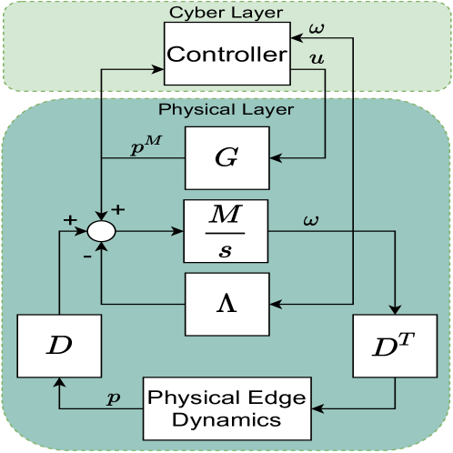
Figure 1: Schematic overview of the power system model. The physical edge dynamics are described by (2a) and (2d). The component $G$ represents the generation dynamics (4) and the controller is to be designed. Though not explicitly illustrated in the figure, it should be noted that the cyber layer is required to be based on a distributed communication protocol so as to implement a distributed secondary frequency control policy.

We adopt the following assumption that is widely used in the power systems literature.

Assumption 2.

$|\eta_{ij}^{*}|<\frac{\pi}{2}$ for all $(i,j)\in E$.

This assumption can be regarded as a security constraint that generally holds under normal operating conditions.

IV Primal-dual Scheme With Communication Delays

In this section, we first review the primal-dual secondary frequency control algorithm for solving the OGR problem (7). Then, we show that the classical scheme is incapable of efficiently incorporating communication delays. Next, we give an equivalent passive reformation of the primal-dual scheme that involves communicating an additional state. This is a key feature that allows to combine the control policy with the scattering transformation so as to achieve delay independent stability.

IV-A Controllers

Equations (10), (11) below describe the primal-dual scheme for optimal secondary frequency control that has been proposed in the literature[3, 4]. In particular, for the generation dynamics (4), the generation input is given by

$$\begin{array}[]{rl}u_{j}=k_{c,j}\left(p_{j}^{c}-\omega_{j}\right)+\frac{p_{j}^{M}}{k_{g,j}}-k_{c,j}Q_{j}^{\prime}\left(p_{j}^{M}\right),~{}j\in G\end{array}$$ (10)

where the parameter $k_{g,j}$ is given in (4), $k_{c,j}>0$, $p_{j}^{c}$ is a control variable through which power sharing is achieved, and is referred to as the power command signal, and $Q_{j}^{\prime}$ represents the gradient of $Q_{j}$ for bus $j$. The dynamics for the power command signal $p_{j}^{c}$ can be found in the literature [3, Eqn (18)] [4, Eqn (6)],

$$\gamma_{ij}\dot{\psi}_{ij}= p_{i}^{c}-p_{j}^{c},~{}(i,j)\in\tilde{E}$$ (11a)

$$\gamma_{j}\dot{p}_{j}^{c}= -\left(p_{j}^{M}-p_{j}^{L}\right)-\sum_{k:j\rightarrow k}\psi_{jk}+\sum_{i:i\rightarrow j}\psi_{ij},~{}j\in N$$ (11b)

where $p_{j}^{M}:=0$, for $j\notin G$, $\gamma_{j}$ and $\gamma_{ij}$ are positive constants, $\psi_{ij}$ is a state of the controller that integrates the power command difference of communicating buses $i$ and $j$. Controller (11) is referred to as ‘virtual swing equation’ [3] since it has a similar structure to that of the system model (2). Equation (11a) can similarly be seen as representing ’virtual edge dynamics’. The set of communication lines $\tilde{E}$ here can be either the same or different to the set of physical transmission lines $E$.

The convergence to an optimal equilibrium point using the control policy in (10), (11) can be found in the literature but we include it here to facilitate the derivation of subsequent results and for completeness.

Lemma 1 (Optimality).

Let Assumption 1 hold. Any equilibrium of system (2), (4), (10), (11) is an optimal solution to the OGR problem (7) with $\omega^{*}=\mathbf{0}_{|N|}$ and $p^{c.*}=\text{Im}(\mathbf{1}_{|N|})$.

The proof can be found in [4].

Lemma 2 (Convergence).

Consider an equilibrium of (2), (4), (10), (11) in which Assumption 2 holds. Then, there exists an open neighborhood about the equilibrium such that solutions of (2), (4), (10), (11) asymptotically converge to a set of equilibria that solve the OGR problem (7) with $\omega^{*}=\mathbf{0}_{|N|}$.

A sketch of the proof is given in Appendix-A.

IV-B Equivalent Reformulation of the Primal-dual Control

Notice that the ‘virtual swing equation’ (11) contains both the virtual bus dynamics (11b) and the virtual edge dynamics (11a). In practice, the virtual edge dynamics (11a) are implemented at each bus; that is, each bus possesses and updates the dynamics of its corresponding edges. As a result, there is redundant information, e.g., the bus $j$ possesses the edge information of $\psi_{ij}$, denoted by $\psi_{ij}^{j}$, while its neighboring bus $i$ possesses the same edge information, denoted by $\psi_{ij}^{i}$. This scheme works satisfactorily in the undelayed case where $\psi_{ij}^{j}=\psi_{ij}^{i}$. However, when there are heterogeneous delays in the communication channel, the updates of the same edge dynamics in the two buses become

$$\gamma_{ij}\dot{\psi}_{ij}^{j}=p_{i}^{c}(t-T_{ij})-p_{j}^{c},~{}(i,j)\in\tilde{E}$$ (12)

$$\gamma_{ij}\dot{\psi}_{ij}^{i}=p_{i}^{c}-p_{j}^{c}(t-T_{ji}),~{}(j,i)\in\tilde{E}$$

where $T_{ij}$ and $T_{ji}$ represents the communication delays in the channel $i\rightarrow j$ and $j\rightarrow i$, respectively. It is apparent that $\psi_{ij}^{j}\neq\psi_{ij}^{i}$, and the goal of the secondary frequency control is not guaranteed, as also illustrated in the simulations in Section VI. Even if we assume in addition that $T_{ij}=T_{ji}$, it still requires the additional knowledge of the delays to update the state with self-induced delays

$$\gamma_{ij}\dot{\psi}_{ij}^{j}=p_{i}^{c}(t-T_{ij})-p_{j}^{c}(t-T_{ij}),~{}(i,j)\in\tilde{E}$$ (13)

such that the two variables ${\psi}_{ij}^{i}$, ${\psi}_{ij}^{j}$ are rendered equal. Moreover, the system becomes unstable when the homogeneous delay is large under this protocol [12].

To ease these restrictions and deal with unknown and heterogeneous delays, we reformulate the primal-dual control algorithm (11) into an equivalent form in which it becomes possible to address delays using the scattering transformation. Let $\gamma_{ij}=\gamma_{j}=1$ in (11) and the communication Laplacian weight in this work be $W=I$ for the ease of presentation, i.e., $\tilde{L}=\tilde{D}\tilde{D}^{T}$, where $\tilde{D}$ is the incidence matrix. We can write (11) into the compact form

$$\dot{\psi}=-\tilde{D}^{T}p^{c},\quad\dot{p}^{c}=-\left(p^{M}-p^{L}\right)+\tilde{D}\psi$$ (14)

where $\psi\in\mathbb{R}^{|\tilde{E}|}$ is the aggregated vector of $\psi_{ij}$, $\forall(i,j)\in\tilde{E}$. Denote $\xi=\tilde{D}\psi$; since $\tilde{D}\tilde{D}^{T}=\tilde{L}$ for undirected communication graphs, (14) becomes

$$\dot{\xi}=-\tilde{L}p^{c},\quad\dot{p}^{c}=-\left(p^{M}-p^{L}\right)+\xi$$ (15)

with initial condition satisfying $\mathbf{1}_{|N|}^{T}\xi(0)=0$ due to $\mathbf{1}_{|N|}^{T}\tilde{D}\psi\equiv 0$. Since $\xi\in\mathbb{R}^{|N|}$, the virtual edge dynamics are thus eliminated and each bus only needs to possess and update the dynamics of $\xi_{j}$ by communicating the variable $p_{j}^{c}$. This reformulation also implies that the primal-dual control (15) in fact inherits a layer of dynamic average consensus dynamics [10]. However, simulations in Section VI show that (15) is problematic under delays because the delayed system will converge to undesirable equilibrium points. This is because in order to have $\mathbf{1}_{|N|}^{T}(p^{M}-p^{L})=0$ at the equilibrium point (which implies $\omega=0$ from (2b)) we need $\mathbf{1}_{|N|}^{T}\xi=0$ at this point, which can be violated if delays are introduced.

To solve this problem, we introduce a coordinate transformation again to reformulate the controller. Notice that the Laplacian $\tilde{L}$ for undirected graphs is positive semidefinite and thus there exists a unique square root $\tilde{L}^{\frac{1}{2}}\geq 0$ such that $\tilde{L}=\tilde{L}^{\frac{1}{2}}\tilde{L}^{\frac{1}{2}}$. Define a new variable $\zeta$ such that $\dot{\zeta}=-\tilde{L}^{\frac{1}{2}}p^{c}$. Then, we have that $\xi=\tilde{L}^{\frac{1}{2}}\zeta$ and (15) becomes

$$\dot{\zeta}=-\tilde{L}^{\frac{1}{2}}p^{c},\quad\dot{p}^{c}=-\left(p^{M}-p^{L}\right)+\tilde{L}^{\frac{1}{2}}\zeta.$$ (16)

Since $\tilde{L}^{\frac{1}{2}}$ is also a well-defined Laplacian matrix, we consider the following new controller for each bus,

$$\dot{\zeta}_{j}= \sum_{i\in\tilde{N}_{j}}\alpha_{ij}\left(p_{i}^{c}-p_{j}^{c}\right),~{}j\in N$$ (17a)

$$\dot{p}_{j}^{c}= -\left(p_{j}^{M}-p_{j}^{L}\right)-\sum_{i\in\tilde{N}_{j}}\alpha_{ij}\left(\zeta_{i}-\zeta_{j}\right),~{}j\in N$$ (17b)

where $\alpha_{ij}>0$ and $\alpha_{ij}=\alpha_{ji}$. Under this controller, the desired relation $\mathbf{1}_{|N|}^{T}(p^{M}-p^{L})=0$ at the equilibrium point is not affected by delays. The only difference between (17) and (16) is in the Laplacian matrices, which do not affect the analysis results as long as the communication graph is connected. Therefore, we have the following corollary.

Corollary 1.

Let Assumption 1 hold and consider an equilibrium of (2), (4), (10), (17) in which Assumption 2 holds. Then, there exists an open neighborhood about the equilibrium such that solutions of (2), (4), (10), (17) converge to a set of equilibria that solve the OGR problem (7) with $\omega^{*}=\mathbf{0}_{|N|}$.

The proof is given in Appendix-B.

As previously discussed, the original controller (11) is incapable of addressing delays efficiently. The significance of the equivalent reformulation (17) that has been derived is that it allows to construct controllers with delay independent stability properties, as it will be shown in the next section. The communication scheme between two buses in (17) is depicted by Fig. 2. It represents the distributed control among buses in the cyber layer of Fig. 1. Note that the buses are also physically coupled in the physical layer but we only include the cyber layer in Fig. 2 to highlight the structure of the communication scheme.

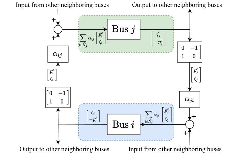
Figure 2: The communication scheme between two buses in the equivalent reformulation (17) of the primal-dual control algorithm. The buses are also coupled in the physical layer, which is not shown here.

Remark 2.

Compared with (11), the reformulations (15) and (17) are both node-based and do not contain virtual edge dynamics. Thus, no redundant update is carried out as in (12). Compared with (15), the reformulation (17) requires communication of the extra variable $\zeta$, but satisfies appropriate passivity properties, which will be shown in the next subsection. The scheme (15) also reveals the existence of a dynamic average consensus control layer [10] underneath the primal-dual scheme. From these forms we can easily observe the difference between the DAPI algorithms [6, 7, 12, 8] and the primal-dual ones, i.e., the former applies the dynamic averaging consensus control directly to the generation input (Equation (32) in [6]) while the latter inherits a layer of dynamic average consensus control within higher-order dynamics.

IV-C Communication Delays and Scattering Transformation

In this subsection we show how the primal-dual secondary control algorithm described in the previous section can be adapted so as to have convergence guarantees when arbitrary heterogeneous delays are present. Suppose that there exist unknown and heterogeneous constant delays in the communication channels between buses. The delay in the communication channel $i\rightarrow j$ is denoted by $T_{ij}$ and the delay in the communication channel $j\rightarrow i$ is denoted by $T_{ji}$, for $(i,j)\in\tilde{E}$.

When there are communication delays in the channel $i\rightarrow j$, $i\in\tilde{N}_{j}$, bus $j$ receives delayed information of $p_{i}^{c}$, $\zeta_{i}$ from bus $i$. Then, controller (17) becomes

$$\begin{array}[]{rl}\dot{\zeta}_{j}=&\displaystyle\sum_{i\in\tilde{N}_{j}}\alpha_{ij}\left(p_{i}^{c}(t-T_{ij})-p_{j}^{c}\right),~{}j\in N\\ \dot{p}_{j}^{c}=&-\left(p_{j}^{M}-p_{j}^{L}\right)-\displaystyle\sum_{i\in\tilde{N}_{j}}\alpha_{ij}\left(\zeta_{i}(t-T_{ij})-\zeta_{j}\right),~{}j\in N\end{array}$$ (20)

which may affect the stability of the power network if delays are large. In fact, the primal-dual controllers are very sensitive to communication delays. Simulations in Section VI show that even some small $T_{ij}$ could destabilize the system.

To deal with communication delays, we start by modifying (17) as

$$\dot{\rho}_{j}^{\zeta}= -\rho_{j}^{\zeta}+\sum_{i\in\tilde{N}_{j}}\alpha_{ij}\left(r_{ij}^{p}-p_{j}^{c}\right),~{}j\in N$$ (21a)

$$\dot{\zeta}_{j}= -\rho_{j}^{\zeta}+2\sum_{i\in\tilde{N}_{j}}\alpha_{ij}\left(r_{ij}^{p}-p_{j}^{c}\right),~{}j\in N$$ (21b)

$$\dot{\rho}_{j}^{p}= {-\rho_{j}^{p}-\left(p_{j}^{M}-p_{j}^{L}\right)-\sum_{i\in\tilde{N}_{j}}\alpha_{ij}\left(r_{ij}^{\zeta}-\zeta_{j}\right),~{}j\in N}$$ (21c)

$$\dot{p}_{j}^{c}= {-\rho_{j}^{p}-2\left(p_{j}^{M}-p_{j}^{L}\right)-2\sum_{i\in\tilde{N}_{j}}\alpha_{ij}\left(r_{ij}^{\zeta}-\zeta_{j}\right),~{}j\in N}$$ (21d)

where $\rho_{j}^{{\zeta}}$, $\rho_{j}^{p}$ are auxiliary states for bus $j$, $r_{ij}^{p}$, $r_{ij}^{\zeta}$ denote information bus $j$ receives from bus $i$. This information will be appropriately formulated via a communication protocol that will be designed in the rest of this section. Equations (21a), (21b) and (21c), (21d) result from the addition of parallel feedforward compensators to (17a), (17b), respectively. It will also be shown later within the paper, that the parallel feedforward compensator provides excess of passivity to guarantee convergence and does not affect the equilibrium since $\rho_{j}^{{\zeta}},{\rho_{j}^{p}}\rightarrow 0$ recovers the original system [22].

Let $\zeta_{j}^{*}$ be an equilibrium value of $\zeta_{j}$ and similarly let $r_{ij}^{p,*},p_{i}^{c,*},r_{ij}^{\zeta,*},\zeta_{i}^{*}$ denote also equilibrium values that satisfy $r_{ij}^{p,*}=p_{i}^{c,*}$, $r_{ij}^{\zeta,*}=\zeta_{i}^{*}$. To facilitate stability analysis under delays, we will utilize an interconnection of passive components. In this regard, we present the following lemma on the passivity of the first component.

Lemma 3.

The system described by (2), (4), (10), (21) is locally passive with respect to input $\begin{bmatrix}\tilde{r}^{p}&\tilde{r}^{\zeta}\end{bmatrix}^{T}$ and output $\begin{bmatrix}\tilde{\zeta}&-\tilde{p}^{c}\end{bmatrix}^{T}$, where the $j^{th}$ element of $\begin{bmatrix}\tilde{r}^{p}&\tilde{r}^{\zeta}\end{bmatrix}^{T}$ and $\begin{bmatrix}\tilde{\zeta}&-\tilde{p}^{c}\end{bmatrix}^{T}$ are defined by $\begin{bmatrix}\tilde{r}_{j}^{p}\\ \tilde{r}_{j}^{\zeta}\end{bmatrix}=\sum_{i\in\tilde{N}_{j}}\alpha_{ij}\left(\begin{bmatrix}r_{ij}^{p}\\ r_{ij}^{\zeta}\end{bmatrix}-\begin{bmatrix}r_{ij}^{p,*}\\ r_{ij}^{\zeta,*}\end{bmatrix}\right)=\sum_{i\in\tilde{N}_{j}}\alpha_{ij}\begin{bmatrix}\tilde{r}_{ij}^{p}\\ \tilde{r}_{ij}^{\zeta}\end{bmatrix}$ and $\begin{bmatrix}\tilde{\zeta}_{j}\\ -\tilde{p}_{j}^{c}\end{bmatrix}=\begin{bmatrix}\zeta_{j}\\ -p_{j}^{c}\end{bmatrix}-\begin{bmatrix}\zeta_{j}^{*}\\ -p_{j}^{c,*}\end{bmatrix},$ respectively.

The proof is given in Appendix-C.

To robustify the communication channels against delays, we send ‘encoded’ information of $\zeta$, $p^{c}$ instead of their direct information, and then ‘decode’ the information received to obtain $\zeta$, $p^{c}$. To this end, we adopt the following scattering transformation

$$s_{\overrightarrow{ij}}=\frac{-1}{\sqrt{2}}\left(\begin{bmatrix}r_{ji}^{p}\\ r_{ji}^{\zeta}\end{bmatrix}-\begin{bmatrix}\zeta_{i}\\ -p_{i}^{c}\end{bmatrix}\right),s_{\overleftarrow{ij}}=\frac{-1}{\sqrt{2}}\left(\begin{bmatrix}r_{ji}^{p}\\ r_{ji}^{\zeta}\end{bmatrix}+\begin{bmatrix}\zeta_{i}\\ -p_{i}^{c}\end{bmatrix}\right)$$ (22)

$$s_{\overleftarrow{ji}}=\frac{1}{\sqrt{2}}\left(\begin{bmatrix}r_{ij}^{p}\\ r_{ij}^{\zeta}\end{bmatrix}+\begin{bmatrix}\zeta_{j}\\ -p_{j}^{c}\end{bmatrix}\right),~{}s_{\overrightarrow{ji}}=\frac{1}{\sqrt{2}}\left(\begin{bmatrix}r_{ij}^{p}\\ r_{ij}^{\zeta}\end{bmatrix}-\begin{bmatrix}\zeta_{j}\\ -p_{j}^{c}\end{bmatrix}\right)$$

where $s_{\overrightarrow{ij}}$ is the scattering variable that bus $i$ sends to bus $j$, and $s_{\overleftarrow{ij}}$ is the scattering variable that bus $i$ receives from bus $j$. The other scattering variables above are defined similarly. Let $E_{s}=\begin{bmatrix}0&-1\\ 1&0\end{bmatrix}$ be a matrix gain that is applied on the transmitted scattering variables. Noting that ($s_{\overrightarrow{ij}}$, $s_{\overleftarrow{ji}}$) and ($s_{\overrightarrow{ji}}$, $s_{\overleftarrow{ij}}$) are the variables in the communication channels $i\rightarrow j$ and $j\rightarrow i$, respectively, it holds that

$$s_{\overleftarrow{ij}}(t)=E_{s}s_{\overrightarrow{ji}}(t-T_{ji}),\quad s_{\overleftarrow{ji}}(t)=E_{s}s_{\overrightarrow{ij}}(t-T_{ij}).$$ (23)

where $T_{ji}$, $T_{ij}$ are delays in the communication channels $j\rightarrow i$ and $i\rightarrow j$, respectively, $s_{\overrightarrow{ji}}(t)=\mathbf{0}$ and $s_{\overrightarrow{ij}}(t)=\mathbf{0}$, $\forall t<0$. The communication process from bus $j$ to $i$ is summarized as follows.

1. Bus $j$ encodes its original input $\begin{bmatrix}r_{ij}^{p}\\ r_{ij}^{\zeta}\end{bmatrix}$ and output $\begin{bmatrix}\zeta_{j}\\ -p_{j}^{c}\end{bmatrix}$ into the scattering variable $s_{\overrightarrow{ji}}$ based on (22).

2. Scattering variable $s_{\overrightarrow{ji}}$ is transmitted in the communication channel $j\rightarrow i$ under delay $T_{ji}$. Then bus $i$ receives $s_{\overleftarrow{ij}}(t)$ given by (23).

3. Bus $i$ decodes the variable $s_{\overleftarrow{ij}}$ and extracts original input $\begin{bmatrix}r_{ji}^{p}\\ r_{ji}^{\zeta}\end{bmatrix}$ based on (22).

The communication from bus $i$ to $j$ is carried out similarly. This communication scheme is depicted in Fig. 3. If there are no delays, i.e., $T_{ij}=T_{ji}=0$, we immediately obtain $r_{ij}^{p}=p_{i}^{c}$, $r_{ij}^{\zeta}=\zeta_{i}$, for all $(i,j)\in\tilde{E}$ since (22), (23) are equivalent to loop transformations in the undelayed case.

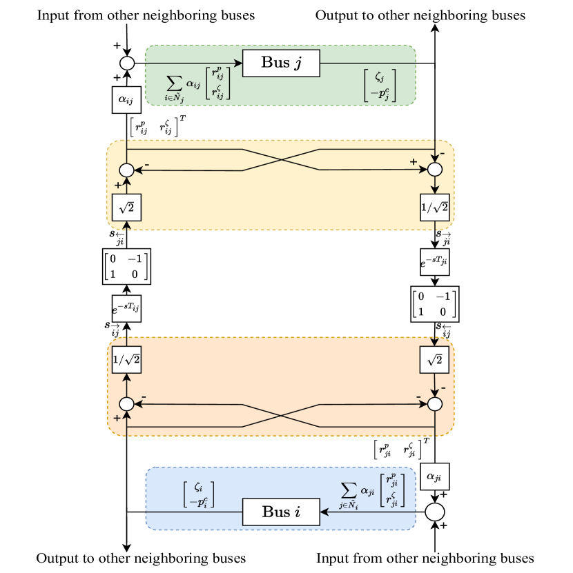
Figure 3: The scattering transformation between two buses under communication delays for the primal-dual scheme. The scattering transformation is passive with respect to the two-port inputs and outputs, as shown in Lemma 4.

Remark 3.

Observe that there exist algebraic loops in the scattering transformation as original inputs and outputs are coupled to construct new inputs and outputs. Eliminating the algebraic loops we obtain

$$\begin{bmatrix}{r}_{ij}^{p}(t)\\ {r}_{ij}^{\zeta}(t)\end{bmatrix}= -\begin{bmatrix}{r}_{ij}^{p}(t-T_{ij}-T_{ji})\\ {r}_{ij}^{\zeta}(t-T_{ij}-T_{ji})\end{bmatrix}+\begin{bmatrix}{\zeta}_{j}(t-T_{ij}-T_{ji})\\ -{p}_{j}^{c}(t-T_{ij}-T_{ji})\end{bmatrix}$$

$$-\begin{bmatrix}{\zeta}_{j}(t)\\ -{p}_{j}^{c}(t)\end{bmatrix}+2\begin{bmatrix}{p}_{i}^{c}(t-T_{ij})\\ {\zeta}_{i}(t-T_{ij})\end{bmatrix}.$$ (24)

The system consisting of (2), (4), (10), (21), (3) becomes a delay differential algebraic equation [14]. Note that solutions trivially exist and are unique for a given initial condition [20, 19].

Remark 4.

Our work differs from the application of scattering transformation to distributed optimization [18], due to the presence of the physical power system dynamics that couple the individual buses, in addition to the coupling arising from the communication between the controllers. The scattering transformation depicted in Fig. 3 involves the communication of two variables and an extra matrix gain $E_{s}$ is added in (23), compared to the way it is commonly used in the literature [15, 17, 18, 16]. The matrix $E_{s}$ appears due to the special structure of interconnection in Fig. 2. This additional matrix does not disrupt the passivity of the system arising from the scattering transformation (Lemma 4 below) since its norm is not greater than one [15]. This formulation of the scattering transformation is more broadly applicable to systems having similar distributed control structures, such as the extensions presented in Section V.

The constructed scattering transformation is the second component of the interconnection of passive components, which is passive with respect to its two-port inputs and outputs as stated in the following lemma.

Lemma 4.

The system described by (22) and (23) is passive with respect to input $\begin{bmatrix}\begin{bmatrix}\tilde{\zeta}_{j}&-\tilde{p}_{j}^{c}\end{bmatrix}&\begin{bmatrix}\tilde{\zeta}_{i}&-\tilde{p}_{i}^{c}\end{bmatrix}\end{bmatrix}^{T}$ and output $-\begin{bmatrix}\begin{bmatrix}\tilde{r}_{ij}^{p}&\tilde{r}_{ij}^{\zeta}\end{bmatrix}&\begin{bmatrix}\tilde{r}_{ji}^{p}&\tilde{r}_{ji}^{\zeta}\end{bmatrix}\end{bmatrix}^{T}$, where these variables are as defined in Lemma 3.

The proof is given in Appendix-D.

IV-D Convergence and Optimality

After showing passivity of the component (2), (4), (10), (21) via Lemma 3, and the component (22), (23) via Lemma 4, respectively, we are ready to prove asymptotic stability of the closed-loop system under arbitrary constant delays.

Theorem 1.

Let Assumption 1 hold, and consider an equilibrium point of system (2), (4), (10), (21), (22), (23) in which Assumption 2 holds. The delays $T_{ij}\geq 0$, $\forall(i,j)\in\tilde{E}$ are assumed to be constant, and are allowed to take arbitrary bounded values and be heterogeneous. Then, there exists an open neighborhood $\Omega$ about this equilibrium point such that the solutions of (2), (4), (10), (21), (22), (23) with initial conditions in $\Omega$ converge to an equilibrium point that solves the OGR problem (7) with $\omega^{*}=\mathbf{0}_{|N|}$.

The proof is given in Appendix-E.

V Extensions

As previously mentioned, the conventional primal-dual controllers can be extended to consider more complex scenarios such as tie-line power flow constraints [3] and generation boundedness constraints [4]. We show in this section that the proposed delay independent primal-dual controllers can also adopt such additional requirements. In particular, we consider additional tie-line power flow constraints, generation boundedness constraints, and then relax the requirement of demand measurements using an observer layer.

V-A Tie-line Power Flow Constraints

Recall that ${C}_{k}$ is the set of buses in the control area $k\in K$. The following OGR-2 problem considers additional tie-line power flow constraints,

$$\begin{array}[]{rl}\textbf{OGR-2:}&\underset{p^{M},p}{\min}~{}\displaystyle\sum_{j\in G}Q_{j}(p_{j}^{M}),\\ &\text{subject to }\displaystyle\sum_{j\in G}p_{j}^{M}=\sum_{j\in N}p_{j}^{L},\\ &\qquad\qquad\displaystyle\sum_{(i,j)\in{B}_{k}}\hat{D}_{k,ij}p_{ij}=\hat{P}_{k},~{}k\in{K}\end{array}$$ (28)

where $\hat{P}_{k}$ is the net power injection of area $k$, ${B}_{k}$ is the set of physical lines that connect area $k$ to other areas, and $\hat{D}_{k,ij}=1$ if $i\in C_{k}$, $\hat{D}_{k,ij}=-1$ if $j\in{C}_{k}$, and $\hat{D}_{k,ij}=0$, otherwise. The second constraint in (28) specifies power transfer between areas. Moreover, let $\hat{D}=[\hat{D}_{k,ij}]\in\mathbb{R}^{|{K}|\times|E|}$ and $E_{{K}}=[e_{1}~{}\ldots~{}e_{|K|}]^{T}\in\mathbb{R}^{|{K}|\times|N|}$, where $e_{k}\in\mathbb{R}^{|N|}$, $k\in K$ is a vector with elements $(e_{k})_{j}=1$ if $j\in C_{k}$ and $(e_{k})_{j}=0$ otherwise. Then, $\hat{D}$ can be related with the incidence matrix ${D}$ by ([3])

$$\hat{D}=E_{{K}}{D}.$$ (29)

Note that solving the OGR-2 problem (28) is challenging since we cannot manipulate the variables $p_{j}^{M}$ or $p_{ij}$ directly but can only rely on controllers for the generation input $u$ to alter their values. Since we are aiming in this work to design controllers with delay independent stability, we adopt the reformulated scheme in Section IV and propose an extension of the primal-dual controller to solve (28). For bus $j$ in the $k^{th}$ control area, we replace the controller (17) with

$$\dot{\zeta}_{j}= \sum_{i\in\tilde{N}_{j}}\alpha_{ij}\left(p_{i}^{c}-p_{j}^{c}\right)-\sum_{i\in\tilde{N}_{j}}{\alpha_{ij}}\left(\pi_{i}-\pi_{j}\right),$$ (30a)

$$\dot{p}_{j}^{c}= -\left(p_{j}^{M}-p_{j}^{L}\right)-\sum_{i\in\tilde{N}_{j}}\alpha_{ij}\left(\zeta_{i}-\zeta_{j}\right),$$ (30b)

$$\dot{\pi}_{j}= \sum_{i\in\tilde{N}_{j}}{\alpha_{ij}}\left(\zeta_{i}-\zeta_{j}\right)-\sum_{i\in\tilde{N}_{j}\cap{C}_{k}}{\alpha_{ij}}\left(\phi_{i}-\phi_{j}\right)-J_{j}\hat{P}_{k},$$ (30c)

$$\dot{\phi}_{j}= \sum_{i\in\tilde{N}_{j}\cap{C}_{k}}{\alpha_{ij}}\left(\pi_{i}-\pi_{j}\right),$$ (30d)

where $\pi_{j}$, $\phi$ are auxiliary variables associated with the tie-line power flow constraints, and $J_{j}\in\{0,1\}$, is a constant representing the knowledge of $\hat{P}_{k}$. In particular, we assume that in the area $k$ only one bus $j_{k}$ has access to the value of $\hat{P}_{k}$ such that $J_{j}=1$ if $j=j_{k}$ and $J_{j}=0$, otherwise. In (30c) and (30d), the use of the set $\tilde{N}_{j}\cap{C}_{k}$ implies that variables $\phi_{j}$ and $\pi_{j}$ are exchanged only within the same control area.

Remark 5.

Compared with [3], controller (30) is proposed without centralized control or virtual edge dynamics such that communication delays can be similarly addressed without the obstacles discussed in Section IV-B. Similar controllers can be found in [9], where an undelayed scheme is analyzed that relaxes the requirement for demand measurements. Compared to [9], our proposed controller (30) does not need to verify conditions that involve global parameters to guarantee stability, and can also be used to achieve stability for arbitrary communication delays as it will be shown in this section.

Let $\tilde{L}_{{K}}$ be the Laplacian matrix for the graph $\mathcal{G}(N,\tilde{E}/\tilde{B})$, where $\tilde{B}$ is the set of inter-area communication lines. Then, algorithm (30) can be written in the compact form

$$\dot{\zeta}= -\tilde{L}p^{c}+\tilde{L}\pi,$$ (31a)

$$\dot{p}^{c}= -\left(p^{M}-p^{L}\right)+\tilde{L}\zeta,$$ (31b)

$$\dot{\pi}= -\tilde{L}\zeta+\tilde{L}_{{K}}\phi-J\hat{P},$$ (31c)

$$\dot{\phi}= -\tilde{L}_{{K}}\pi,$$ (31d)

where $J=[J_{i,j}]\in\mathbb{R}^{|N|\times|{K}|}$ with $J_{j_{k},k}=1$ and $J_{j_{k},k}=0$ otherwise, and $\hat{P}=\left(\hat{P}_{1},\ldots,\hat{P}_{|{K}|}\right)^{T}$.

We first show the optimality of the control algorithm.

Lemma 5 (Optimality).

Let Assumption 1 hold. Any equilibrium of system (2), (4), (10), (30) is an optimal solution to the OGR-2 problem (28) with $\omega^{*}=\mathbf{0}_{|N|}$.

The proof is provided in Appendix-F.

When there are communication delays in the channel $i\rightarrow j$, $i\in\tilde{N}_{j}$, bus $j$ receives delayed information of $p_{i}^{c}$, $\zeta_{i}$, $\pi_{i}$ and $\phi_{i}$ from bus $i$. Then, controller (30) becomes

$$\dot{\zeta}_{j}= \sum_{i\in\tilde{N}_{j}}\alpha_{ij}\left(p_{i}^{c}(t-T_{ij})-p_{j}^{c}\right)-\sum_{i\in\tilde{N}_{j}}{\alpha_{ij}}\left(\pi_{i}(t-T_{ij})-\pi_{j}\right),$$ (32a)

$$\dot{p}_{j}^{c}= -\left(p_{j}^{M}-p_{j}^{L}\right)-\sum_{i\in\tilde{N}_{j}}\alpha_{ij}\left(\zeta_{i}(t-T_{ij})-\zeta_{j}\right),$$ (32b)

$$\dot{\pi}_{j}= \sum_{i\in\tilde{N}_{j}}\alpha_{ij}\left(\zeta_{i}(t-T_{ij})-\zeta_{j}\right)-\sum_{i\in\tilde{N}_{j}\cap{C}_{k}}{\alpha_{ij}}\left(\phi_{i}(t-T_{ij})-\phi_{j}\right)-J_{j}\hat{P}_{k},$$ (32c)

$$\dot{\phi}_{j}= \sum_{i\in\tilde{N}_{j}\cap{C}_{k}}{\alpha_{ij}}\left(\pi_{i}(t-T_{ij})-\pi_{j}\right),$$ (32d)

for all $j\in N$, if variables are directly communicated. The delays may destabilize the system if they are large.

To deal with communication delays, we modify the controllers (30) as

$$\begin{array}[]{rl}\dot{\rho}_{j}^{{\zeta}}=&-\rho_{j}^{{\zeta}}+\displaystyle\sum_{i\in\tilde{N}_{j}}\alpha_{ij}\left(r_{ij}^{p}-p_{j}^{c}\right)-\displaystyle\sum_{i\in\tilde{N}_{j}}{\alpha_{ij}}\left(r_{ij}^{\pi^{\prime}}-\pi_{j}\right),\\ \dot{\zeta}_{j}=&-\rho_{j}^{{\zeta}}+2\displaystyle\sum_{i\in\tilde{N}_{j}}\alpha_{ij}\left(r_{ij}^{p}-p_{j}^{c}\right)-2\displaystyle\sum_{i\in\tilde{N}_{j}}{\alpha_{ij}}\left(r_{ij}^{\pi^{\prime}}-\pi_{j}\right),\\ \dot{\rho}_{j}^{p}=&{-\rho_{j}^{p}-\left(p_{j}^{M}-p_{j}^{L}\right)-\displaystyle\sum_{i\in\tilde{N}_{j}}\alpha_{ij}\left(r_{ij}^{\zeta}-\zeta_{j}\right),}\\ \dot{p}_{j}^{c}=&{-\rho_{j}^{p}-2\left(p_{j}^{M}-p_{j}^{L}\right)-2\displaystyle\sum_{i\in\tilde{N}_{j}}\alpha_{ij}\left(r_{ij}^{\zeta}-\zeta_{j}\right),}\\ \dot{\rho}_{j}^{\pi}=&-\rho_{j}^{\pi}+\displaystyle\sum_{i\in\tilde{N}_{j}}{\alpha_{ij}}\left(r_{ij}^{\zeta^{\prime}}-\zeta_{j}\right)-\displaystyle\sum_{i\in\tilde{N}_{j}\cap{C}_{k}}{\alpha_{ij}}\left(r_{ij}^{\phi^{\prime\prime}}-\phi_{j}\right)-J_{j}\hat{P}_{k},\\ \dot{\pi}_{j}=&-\rho_{j}^{\pi}+2\displaystyle\sum_{i\in\tilde{N}_{j}}{\alpha_{ij}}\left(r_{ij}^{\zeta^{\prime}}-\zeta_{j}\right)-2\displaystyle\sum_{i\in\tilde{N}_{j}\cap{C}_{k}}{\alpha_{ij}}\left(r_{ij}^{\phi^{\prime\prime}}-\phi_{j}\right)-2J_{j}\hat{P}_{k},\\ \dot{\rho}_{j}^{\phi}=&-\rho_{j}^{\phi}+\displaystyle\sum_{i\in\tilde{N}_{j}\cap{C}_{k}}{\alpha_{ij}}\left(r_{ij}^{\pi^{\prime\prime}}-\pi_{j}\right),\\ \dot{\phi}_{j}=&-\rho_{j}^{\phi}+2\displaystyle\sum_{i\in\tilde{N}_{j}\cap{C}_{k}}{\alpha_{ij}}\left(r_{ij}^{\pi^{\prime\prime}}-\pi_{j}\right),\\[-5.69054pt] \end{array}$$ (41)

for all $j\in N$ and $j\in C_{k}$, where $\rho_{j}^{\zeta}$, $\rho_{j}^{p}$, $\rho_{j}^{\pi}$, $\rho_{j}^{\phi}$ are auxiliary states resulting from parallel feedforward compensation on (30), similarly to (21). As (30) has three pairs of communication variables, there are three sets of scattering transformations, and $r_{ij}^{p}$, $r_{ij}^{\zeta}$, $r_{ij}^{\zeta^{\prime}}$, $r_{ij}^{\pi^{\prime}}$, $r_{ij}^{\pi^{\prime\prime}}$, $r_{ij}^{\phi^{\prime\prime}}$ represent variables bus $j$ formulates using the information communicated from bus $i$. The above extended algorithm also inherits passivity properties. As in Lemma 3 the superscript ^∗ in Lemma 6 below is used to denote values at an equilibrium point.

Lemma 6.

The system described by (2), (4), (10), (41) is locally passive from input $\begin{bmatrix}\tilde{r}^{p}&\tilde{r}^{\zeta}&\tilde{r}^{\zeta^{\prime}}&\tilde{r}^{\pi^{\prime}}&\tilde{r}^{\pi^{\prime\prime}}&\tilde{r}^{\phi^{\prime\prime}}\end{bmatrix}^{T}$ to output $\begin{bmatrix}\tilde{\zeta}&-\tilde{p}^{c}&\tilde{\pi}&-\tilde{\zeta}&\tilde{\phi}&-\tilde{\pi}\end{bmatrix}^{T}$, where the $j^{th}$ element of the variables are defined by

$$\left[\begin{smallmatrix}\tilde{r}_{j}^{p}&\tilde{r}_{j}^{\zeta}&\tilde{r}_{j}^{\zeta^{\prime}}&\tilde{r}_{j}^{\pi^{\prime}}\end{smallmatrix}\right]^{T}=\sum_{i\in\tilde{N}_{j}}\alpha_{ij}\left[\begin{smallmatrix}r_{ij}^{p}-r_{ij}^{p,*}&r_{ij}^{\zeta}-r_{ij}^{\zeta,*}&r_{ij}^{\zeta^{\prime}}-r_{ij}^{\zeta,*}&r_{ij}^{\pi^{\prime}}-r_{ij}^{\pi,*}\end{smallmatrix}\right]^{T},$$

$$\left[\begin{smallmatrix}\tilde{r}_{j}^{\pi^{\prime\prime}}&\tilde{r}_{j}^{\phi^{\prime\prime}}\end{smallmatrix}\right]^{T}=\sum_{i\in\tilde{N}_{j}\cap{C}_{k}}\alpha_{ij}\left[\begin{smallmatrix}r_{ij}^{\pi^{\prime\prime}}-r_{ij}^{\pi,*}&r_{ij}^{\phi^{\prime\prime}}-r_{ij}^{\phi,*}\end{smallmatrix}\right]^{T},~{}{j\in C_{k}},$$

$$\left[\begin{smallmatrix}\tilde{\zeta}_{j}&\tilde{p}_{j}^{c}&\tilde{\pi}_{j}&\tilde{\phi}_{j}\end{smallmatrix}\right]^{T}=\left[\begin{smallmatrix}\zeta_{j}-\zeta_{j}^{*}&p_{j}^{c}-p_{j}^{c,*}&\pi_{j}-\pi_{j}^{*}&\pi_{j}-\phi_{j}^{*}\end{smallmatrix}\right]^{T}$$

The proof is given in Appendix-G.

Remark 6.

The input and output in Lemma 6 contain repeated variables. This may appear redundant, but they are formulated in this way such that one can construct a passive scattering transformation for the communication channel.

We now define a new set of scattering variables, which are the variables that get communicated between buses. Let $r_{ji}=\left({r}^{p}_{ji},{r}^{\zeta}_{ji},{r}^{\zeta^{\prime}}_{ji},{r}^{\pi^{\prime}}_{ji},\sigma_{ji}{r}^{\pi^{\prime\prime}}_{ji},\sigma_{ji}{r}^{\phi^{\prime\prime}}_{ji}\right)^{T}$ and $y_{ji}=\left(\zeta_{i},-p_{i}^{c},\pi_{i},-\zeta_{i},\sigma_{ji}\phi_{i},-\sigma_{ji}\pi_{i}\right)^{T}$, where $\sigma_{ji}=0$ if $(i,j)\in\tilde{B}$ or $(j,i)\in\tilde{B}$, and $\sigma_{ji}=1$ otherwise. The new scattering variables are given by

$$s_{\overrightarrow{ij}}=-\frac{1}{\sqrt{2}}\left(r_{ji}-y_{ji}\right),~{}s_{\overleftarrow{ij}}=-\frac{1}{\sqrt{2}}\left(r_{ji}+y_{ji}\right)$$ (42)

$$s_{\overleftarrow{ji}}=\frac{1}{\sqrt{2}}\left(r_{ij}+y_{ij}\right),~{}s_{\overrightarrow{ji}}=\frac{1}{\sqrt{2}}\left(r_{ij}-y_{ij}\right).$$

Since $(s_{\overrightarrow{ij}},~{}s_{\overleftarrow{ji}})$ and $(s_{\overrightarrow{ji}},~{}s_{\overleftarrow{ij}})$ are the variables in the communication channels $i\rightarrow j$ and $j\rightarrow i$, respectively, it holds that

$$s_{\overleftarrow{ij}}(t)=E_{s}s_{\overrightarrow{ji}}(t-T_{ji}),\quad s_{\overleftarrow{ji}}(t)=E_{s}s_{\overrightarrow{ij}}(t-T_{ij})$$ (43)

where $T_{ji}$, $T_{ij}\geq 0$ are delays in the communication channels $j\rightarrow i$ and $i\rightarrow j$, respectively. We also define the matrix gain $E_{s}=I_{3}\otimes\begin{bmatrix}0&-1\\ 1&0\end{bmatrix}$. The new scattering transformation contains three groups of input and output variables, and is analogous to the one used in the previous section. Therefore, it is also passive, as stated below.

Lemma 7.

The system described by (42) and (43) is passive from input $\begin{bmatrix}\tilde{y}_{ij}\\ \tilde{y}_{ji}\end{bmatrix}$ to output $-\begin{bmatrix}\tilde{r}_{ij}\\ \tilde{r}_{ji}\end{bmatrix}$ where $\tilde{r}_{ij}=r_{ij}-r_{ij}^{*}$ and $\tilde{y}_{ij}=y_{ij}-y_{ij}^{*}$.

The proof is given in Appendix-H.

Using the passivity of the two components (2), (4), (10), (41), and (42), (43) stated in Lemma 6 and Lemma 7, respectively, we are ready to deduce asymptotic stability of the closed-loop system under arbitrary constant delays.

Theorem 2.

Let Assumption 1 hold and consider an equilibrium point of system (2), (4), (10), (41), (42), (43) in which Assumption 2 holds. The delays $T_{ij}\geq 0$, $\forall(i,j)\in\tilde{E}$ are assumed to be constant, and are allowed to take arbitrary bounded values and be heterogeneous. Then, there exists an open neighborhood $\Omega$ about this equilibrium point such that the solutions of (2), (4), (10), (41), (42), (43) with initial conditions in $\Omega$ converge to an equilibrium point that solves the OGR-2 problem (28) with $\omega^{*}=\mathbf{0}_{|N|}$.

The proof is given in Appendix-I.

V-B Generation Boundedness Constraints

In this subsection, we consider bounds for the minimum and maximum values of generation to account for a more realistic operating condition.

$$\begin{array}[]{rl}\textbf{OGR-3:}&\underset{p^{M}}{\min}\displaystyle\sum_{j\in G}Q_{j}(p_{j}^{M}),\\ &\text{subject to }\displaystyle\sum_{j\in G}p_{j}^{M}=\sum_{j\in N}p_{j}^{L},\\ &p_{j}^{M,\min}\leq p_{j}^{M}\leq p_{j}^{M,\max},\forall j\in G,\end{array}$$ (47)

where $p_{j}^{M,\min}$, $p_{j}^{M,\max}$ are lower and upper bounds for the for generation at bus $j$.

In the undelayed case, a function with saturation can be used to modify the generation input so as to satisfy thee generation bounds at equilibrium [4]. In order, however, to avoid complications associated with a non-smooth vector field in an infinite dimensional setting associated with delays, we use below an alternative scheme that leads to smooth dynamics.

In particular, to solve the OGR-3 problem (47), the controller (21) is left unchanged, while the generation input (10) is changed to

$$u_{j}=k_{c,j}\left(p_{j}^{c}-\omega_{j}\right)+\frac{p_{j}^{M}}{k_{g,j}}-k_{c,j}\left(Q_{j}^{\prime}\left(p_{j}^{M}\right)-\lambda_{j}^{2}+\mu_{j}^{2}\right),~{}j\in G$$ (48)

where $\lambda_{j}^{2}$, $\mu_{j}^{2}$ can be viewed as non-negative Lagrange multipliers for the inequalities. The variables $\lambda_{j}$, $\mu_{j}$ follow the dynamics

$$\dot{\lambda}_{j}=2\lambda_{j}\left(p_{j}^{M,\min}-p_{j}^{M}\right),~{}\lambda_{j}(0)>0,$$ (49a)

$$\dot{\mu}_{j}=2\mu_{j}\left(p_{j}^{M}-p_{j}^{M,\max}\right),~{}\mu_{j}(0)>0.$$ (49b)

The update rule (49) is used here as a means of solving an inequality constrained optimization problem with smooth dynamics [23]. We show below that optimality and convergence are guaranteed by the augmented dynamics described above.

Lemma 8 (Optimality).

Let Assumption 1 hold. Any equilibrium of system (2), (4), (11), (48), (49) is an optimal solution to the OGR-3 problem (47) with $\omega^{*}=\mathbf{0}_{|N|}$ and $p^{c,*}=\text{Im}(\mathbf{1}_{|N|})$.

The proof is given in Appendix-J.

The stability of the primal-dual controlled system considered that incorporates generation bounds and delays is stated in the Theorem below.

Theorem 3.

Let Assumption 1 hold and consider an equilibrium point of system (2), (4), (21), (22), (23), (48), (49), in which Assumption 2 holds. The delays $T_{ij}\geq 0$, $\forall(i,j)\in\tilde{E}$ are assumed to be constant, and are allowed to take arbitrary bounded values and be heterogeneous. Then, there exists an open neighborhood $\Omega$ about this equilibrium point such that the solutions of (2), (4), (21), (22), (23), (48), (49) with initial conditions in $\Omega$ converge to an equilibrium point that solves the OGR-3 problem (47) with $\omega^{*}=\mathbf{0}_{|N|}$.

The proof is given in Appendix-K.

Remark 7.

It should be noted that the dynamics in (49) follow from the dual gradient ascent of the generalized Lagrangian

$$\mathcal{L}=\sum_{j\in G}Q_{j}\left(p_{j}^{M}\right)+\lambda_{j}^{2}\left(p_{j}^{M,\min}-p_{j}^{M}\right)+\mu_{j}^{2}\left(p_{j}^{M}-p_{j}^{M,\max}\right)$$ (50)

V-C Observer-based Estimation for Demand

The control strategy proposed in (21), (22), (23) requires the explicit knowledge of the uncontrollable frequency independent demand $p^{L}$. In this subsection, we include observer dynamics borrowed from [4] to relax this requirement without affecting the stability and optimality presented in Theorem 1. The controller under observer dynamics is

$$\dot{\rho}_{j}^{{\zeta}}=-\rho_{j}^{{\zeta}}+\sum_{i\in\tilde{N}_{j}}\alpha_{ij}\left(r_{ij}^{p}-p_{j}^{c}\right),~{}j\in N$$ (51a)

$$\dot{\zeta}_{j}=-{\rho_{j}^{\zeta}}+2\sum_{i\in\tilde{N}_{j}}\alpha_{ij}\left(r_{ij}^{p}-p_{j}^{c}\right),~{}j\in N$$ (51b)

$${\dot{\rho}_{j}^{p}=-{\rho}_{j}^{p}-\left(p_{j}^{M}-\chi_{j}\right)-\sum_{i\in\tilde{N}_{j}}\alpha_{ij}\left(r_{ij}^{\zeta}-\zeta_{j}\right),~{}j\in N}$$ (51c)

$$\dot{p}_{j}^{c}=-{{\rho}_{j}^{p}-2\left(p_{j}^{M}-\chi_{j}\right)-2\sum_{i\in\tilde{N}_{j}}\alpha_{ij}\left(r_{ij}^{\zeta}-\zeta_{j}\right),~{}j\in N}$$ (51d)

$$\tau_{\chi,j}\dot{\chi}_{j}=b_{j}-\omega_{j}-p_{j}^{c}-\chi_{j},~{}j\in G$$ (51e)

$$M_{j}\dot{b}_{j}=-\chi_{j}+p_{j}^{M}-\Lambda_{j}\omega_{j}-\sum_{k:j\rightarrow k}p_{jk}+\sum_{i:i\rightarrow j}p_{ij},~{}j\in G$$ (51f)

$$0=-\chi_{j}-\Lambda_{j}\omega_{j}-\sum_{k:j\rightarrow k}p_{jk}+\sum_{i:i\rightarrow j}p_{ij},~{}j\in L$$ (51g)

The stability of the primal-dual controlled system relaxing demand measurement under delays is given as follows.

Theorem 4.

Let Assumption 1 hold and consider an equilibrium point of system (2), (4), (10), (51), (22), (23) in which Assumption 2 holds. The delays $T_{ij}\geq 0$, $\forall(i,j)\in\tilde{E}$ are assumed to be constant, and are allowed to take arbitrary bounded values and be heterogeneous. Then, there exists an open neighborhood $\Omega$ about this equilibrium point such that the solutions of (2), (4), (10), (51) , (22), (23) with initial conditions in $\Omega$ converge to an equilibrium point that solves the OGR problem (7) with $\omega^{*}=\mathbf{0}_{|N|}$.

The proof is given in Appendix-L.

Note that we do not include delays in the observer layer (51e), (51f), (51g) for simplicity in the presentation. If delays in the estimation of $p_{ij}$ are considered, a similar controller incorporating a scattering transformation can be readily constructed. It is also worth noting that the three extensions in Sections V-A, V-B and V-C can be easily combined together, while still maintaining the optimality and convergence properties that have been derived in the paper. They are presented separately here for brevity and to facilitate readability.

VI Simulations

In this section, we illustrate our results with simulations on a 5-bus example and then on the IEEE-39 test system.

Example 1

Consider a $5$-bus power network example with three generators and two control areas, as shown in Fig. 4.

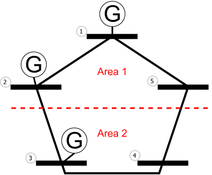
Figure 4: A $5$-bus power network example with three generators and two control areas.

The cost functions are $Q_{j}(p_{j}^{M})=\frac{1}{2}q_{j}\left(p_{j}^{M}-c_{j}\right)^{2}$, $j\in G$. The bus parameters are given in Table II. Let $k_{g,j}=1$, $k_{c,j}=1$, $\forall j\in N$.

Bus	1	2	3	4	5
$q_{j}$	2.4	4	3.4	–	–
$c_{j}$	0.3	0.1	0.2	–	–
$M_{j}$	13	12.1	14.3	–	–
$\tau_{j}$	0.3	0.4	0.35	–	–
$\Lambda_{j}$	1	0.8	1.1	1	0.9
$p^{L}_{j}$	0.1	0.2	0.3	0.4	0.5

TABLE II: Bus parameters.

The loads $p^{L}$ are added at time $t=5s$. The tie-line power flow is scheduled to be $\hat{P}=[-0.5,0.5]$, which is only known to bus $2$ and $3$.

We first show that the primal-dual controllers in the original formulation (11) and the form (15) are incapable of incorporating communication delays efficiently, though they only require communication of the power command signal. As discussed in Section IV-B, the controller (11a) under communication delays becomes (12) with $T_{ij}$ representing the delay in the communication channel $i\rightarrow j$, while the controller (15) under communication delays becomes

$$\dot{\xi}_{j}=\sum_{i\in\tilde{N}_{j}}\alpha_{ij}\left(p_{i}^{c}(t-T_{ij})-p_{j}^{c}\right),~{}\dot{p}_{j}^{c}=-\left(p_{j}^{M}-p_{j}^{L}\right)+\xi_{j},$$ (52)

for all $j\in N$, with initial conditions $\sum_{j\in N}\zeta_{j}(0)=0$. The performance under controllers (12), (11b) and (52) with $T_{ij}=0.01s$, $\forall i,~{}j$, are shown in Fig. 5. We can observe that small delays affect the equilibrium and the frequency is not restored to the nominal value.

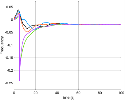
(a) Frequencies under controller (12), (11b).

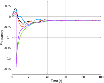
(b) Frequencies under controller (52).

Figure 5: The frequency at each of the buses in Example 1 when the primal-dual control policies (12), (11b) and (52), respectively, are implemented with $T_{ij}=0.01s$.

Next, the performance of the reformulated primal-dual control algorithm (17) and its extension (30) considering tie-line power flow constraints are shown in Fig. 6. It can be observed from Figs. 6(a) and 6(b) that the original controllers (17) and (30) are sensitive to even small delays. On the other hand, when combined with the scattering transformation, the primal-dual controllers can deal with arbitrary bounded, heterogeneous, and unknown delays.

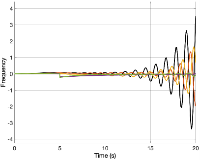
(a) Controller (20) with delays $T_{ij}=0.03s$.

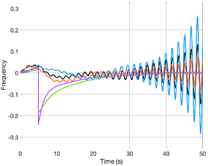
(b) Controller (32) with delays $T_{ij}=0.03s$.

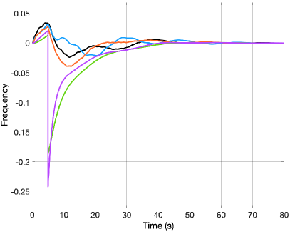
(c) Controller (17) without delays.

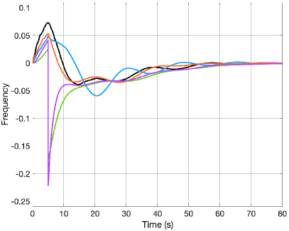
(d) Controller (21) with scattering transformation (22), (23) under delays $T_{ij}\in(0.1,1)s$.

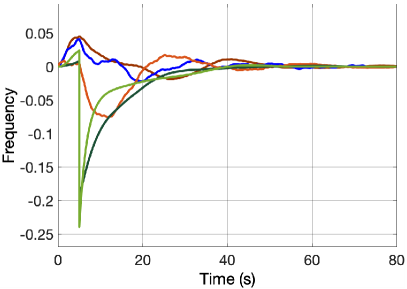
(e) Controller (30) without delays.

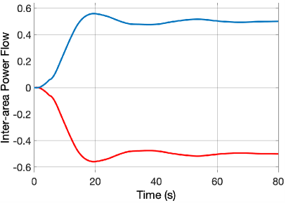
(f) Controller (30) without delays.

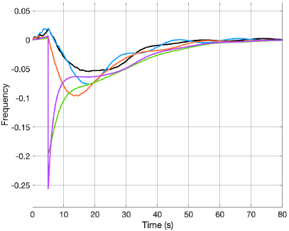
(g) Extended controller (41) with scattering transformation (42), (43) under delays $T_{ij}\in(0.1,1)s$.

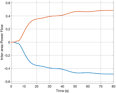
(h) Extended controller (41) with scattering transformation (42), (43) under delays $T_{ij}\in(0.1,1)s$.

Figure 6: Frequencies and inter-area power flows for the primal-dual controllers.

In addition, we show that the control policy with the scattering transformation implemented leads to better disturbance rejection properties also when delays are small. Consider the same $5$-bus power network and assume that there exist disturbances in the communicating between buses, with $d_{ij}$ representing the external disturbance in the channel $i\rightarrow j$. Then, we have

$$s_{\overleftarrow{ij}}(t)=E_{s}s_{\overrightarrow{ji}}(t-T_{ji})+d_{ji},~{}s_{\overleftarrow{ji}}(t)=E_{s}s_{\overrightarrow{ij}}(t-T_{ij})+d_{ij}$$ (53)

in (23) for the primal-dual controller incorporated with scattering transformation, and

$$\begin{bmatrix}p_{i}^{c}&\zeta_{i}\end{bmatrix}^{T}\leftarrow\begin{bmatrix}p_{i}^{c}&\zeta_{i}\end{bmatrix}^{T}+d_{ij}\begin{bmatrix}1&1\end{bmatrix}^{T}$$ (54)

in (17) for the reformulated primal-dual controller without scattering transformation. The frequency response at each bus under square integrable disturbance $d_{ij}=\frac{1}{e_{ij}+t}$, $e_{ij}\in(0,1)$ are shown with and without the scattering transform in Figs. 7(a) and 7(b), respectively, where the former reacts slowly and the latter quickly restores the frequency to the nominal value. The frequency responses when $d_{ij}$ is AWGN with noise power $0.01$ are shown in Figs. 7(c) and 7(d). Note that we only show the disturbance rejection performance of (17) instead of the original one (11) which is unstable for even very small disturbance $d_{ij}$ added to $p_{j}^{c}$. Moreover, we have tried various parameters for the algorithm without scattering transformation, and these do not give significant improvement on the performance in Figs. 7(a) and 7(c). Overall, the primal-dual controller with scattering transformation provides better performance under various types of external disturbances.

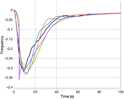
(a) $d_{ij}=\frac{1}{e_{ij}+t}$ without scattering transformation.

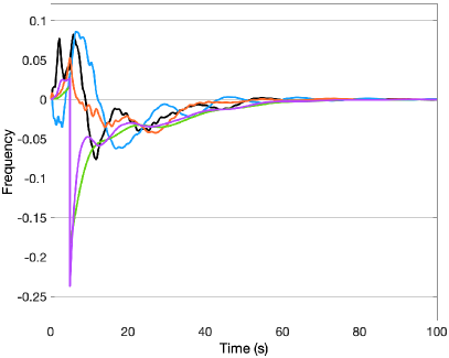
(b) $d_{ij}=\frac{1}{e_{ij}+t}$ with scattering transformation.

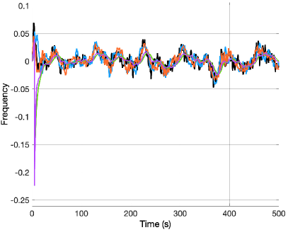
(c) $d_{ij}$ is AWGN with noise power $0.01$, without scattering transformation.

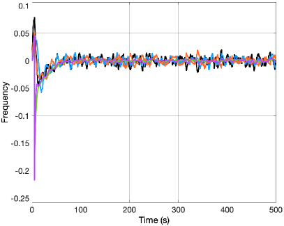
(d) $d_{ij}$ is AWGN with noise power $0.01$, with scattering transformation.

Figure 7: Frequencies for the primal-dual controller (17) under disturbances in the communicated variables described by (53) and (54), respectively, with (right) and without (left) scattering transformation.

Example 2

We apply the proposed secondary frequency control algorithms on the well-known IEEE New England 39-bus system [24]. The model is highly detailed and includes high-order models of the generators, turbine-governors, exciters, transformers and lines. We compare the controller (21) with scattering transformation (22), (23) to the primal-dual scheme (20) under a uniform delay of $T_{ij}=0.02s$. Fig. 8 shows that the controller with scattering transformation is able to tolerate this small delay, unlike the original primal-dual scheme without scattering transform.

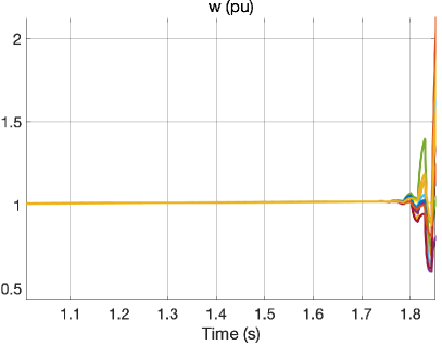
(a) Controller (20) without scattering transformation under delay $T_{ij}=0.02s$.

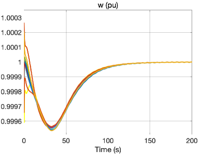
(b) Controller (21) with scattering transformation (22), (23) under delay $T_{ij}=0.02s$.

Figure 8: Frequencies of the ten machines of the IEEE-39 test system under various secondary controllers and delay $T_{ij}=0.02s$.

We also show the ability of the primal-dual controller with scattering transformation to regulate inter-area flows in the presence of delays. To demonstrate this, we designate buses 21-24, 35 and 36 as Area 2 (with the rest of the network as Area 1) and set the total desired inter-area power flow (over two tie-lines) to 450 MW (without the constraint, the steady-state inter-area power-flow is 507 MW). It can be seen from Fig. 9 that the inter-area power-flow is successfully regulated to (very close to) the desired value and the optimal solution to the OGR-2 problem (28) is reached. These examples on a realistic and highly detailed model serve to verify the effectiveness of the proposed primal-dual controller with scattering transformation.

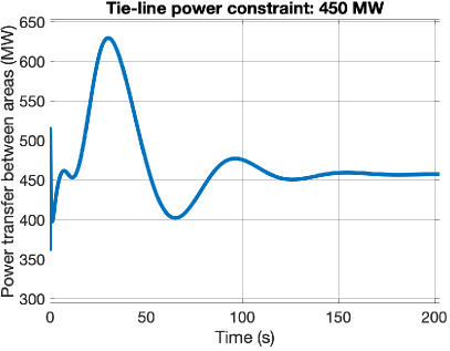
(a) Controller (30) without delays.

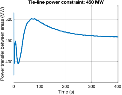
(b) Extended controller (41) with scattering transformation (42), (43) under delays $T_{ij}=0.02s$.

Figure 9: Inter-area power flows for the primal-dual controllers in the IEEE 39 bus system.

VII Conclusion

This work has proposed primal-dual controllers with delay independent stability for distributed secondary frequency control in power systems with unknown and heterogeneous constant communication delays. An equivalent passive reformulation of the controller has been derived and a novel form of passivity-based scattering transformation has been constructed to robustify the closed loop dynamics against communication delays. Moreover, it has been shown that the proposed controllers with delay independent stability properties can adopt various extensions associated with primal-dual control schemes that allow to incorporate various operational constraints. These include extra tie-line power flow and generation boundedness constraints, and a relaxation of the requirement for demand measurements via an observer.

Appendix

-A Proof of Lemma 2

Proof.

Consider the Lyapunov function candidate

$$V_{pd}=V_{F}\left(\omega^{G}\right)+V_{P}(\eta)+V_{C}\left(p^{c}\right)+V_{\psi}\left(\psi\right)+V_{D}\left(p^{M}\right)$$ (55)

where the functions on the right hand side are defined by

$$V_{F}(\omega^{G})=\frac{1}{2}\sum_{j\in G}M_{j}\left(\omega_{j}-\omega_{j}^{*}\right)^{2}\geq 0,$$ (56)

$$V_{P}(\eta)=\sum_{(i,j)\in E}Y_{ij}\int_{\eta_{ij}^{*}}^{\eta_{ij}}\left(\sin\theta-\sin\eta_{ij}^{*}\right)d\theta,$$ (57)

$$V_{C}(p^{c})=\frac{1}{2}\sum_{j\in N}\gamma_{j}\left(p_{j}^{c}-p_{j}^{c,*}\right)^{2}\geq 0,$$ (58)

$$V_{\psi}(\psi)=\sum_{(i,j)\in\tilde{E}}\frac{1}{2}\gamma_{ij}\left(\psi_{ij}-\psi_{ij}^{*}\right)^{2}\geq 0,$$ (59)

$$V_{D}(p^{M})=\sum_{j\in G}\frac{\tau_{j}}{2k_{g,j}k_{c,j}}\left(p_{j}^{M}-p_{j}^{M,*}\right)^{2}\geq 0,$$ (60)

respectively, and $V_{P}\geq 0$ in some neighborhood of $\eta^{*}$ as follows from Assumption 2. The time derivative of $V_{pd}$ along the system trajectories satisfies

$$\begin{array}[]{rl}\dot{V}_{pd}=&-\sum_{j\in N}\Lambda_{j}\left(\omega_{j}-\omega_{j}^{*}\right)^{2}\\ &-\sum_{j\in G}\left(Q_{j}^{\prime}\left(p_{j}^{M}\right)-Q_{j}^{\prime}\left(p_{j}^{M,*}\right)\right)\left(p_{j}^{M}-p_{j}^{M,*}\right)\leq 0.\end{array}$$

The rest of the proof can be found in [4]. ∎

-B Proof of Corollary 1

Consider the Lyapunov function candidate

$$V_{N}=V_{F}\left(\omega^{G}\right)+V_{P}(\eta)+V_{C}\left(p^{c}\right)+V_{D}\left(p^{M}\right)+V_{\zeta}(\zeta)$$

where $V_{F}\left(\omega^{G}\right)$, $V_{P}(\eta)$, $V_{C}\left(p^{c}\right)$, and $V_{D}\left(p^{M}\right)$ are defined by (56), (57), (58), and (60), respectively, and $V_{\zeta}=\frac{1}{2}\sum_{j\in N}\left(\zeta_{j}-\zeta_{j}^{*}\right)^{2}$. The rest of the proof are similar to the proof of Lemma 2.

-C Proof of Lemma 3

Proof.

Adopt the storage function

$$V_{B}=V_{F}\left(\omega^{G}\right)+V_{P}(\eta)+{V_{p^{c},\rho}\left(p^{c},\rho^{p}\right)}+V_{D}\left(p^{M}\right)+V_{\zeta,\rho}(\zeta,\rho^{\zeta})$$ (61)

where $V_{F}\left(\omega^{G}\right)$, $V_{P}(\eta)$ and $V_{D}\left(p^{M}\right)$ are defined by (56), (57), and (60), respectively, and

$$\begin{array}[]{rl}V_{p^{c},\rho}(p^{c},\rho^{p})=\displaystyle\frac{1}{2}(\rho_{j}^{p})^{2}+\frac{1}{2}\sum_{j\in N}\left(p_{j}^{c}-\rho_{j}^{p}-p_{j}^{c,*}\right)^{2},\\ V_{\zeta,\rho}(\zeta,\rho^{\zeta})=\displaystyle\frac{1}{2}(\rho_{j}^{\zeta})^{2}+\frac{1}{2}\sum_{j\in N}\left(\zeta_{j}-\rho_{j}^{\zeta}-\zeta_{j}^{*}\right)^{2}.\end{array}$$

By Assumption 2, there exists an open neighborhood of $\eta^{*}$ such that $V_{B}\geq 0$. The time derivative of $V_{B}$ along the system trajectories is given by

$$\begin{array}[]{rl}\dot{V}_{B}=&-\sum_{j\in N}\left(\Lambda_{j}\left(\omega_{j}-\omega_{j}^{*}\right)^{2}+{(\rho_{j}^{p})^{2}+(\rho_{j}^{\zeta})^{2}}\right)\\ &-\sum_{j\in G}\left(p_{j}^{M}-p_{j}^{M,*}\right)\left(Q_{j}^{\prime}\left(p_{j}^{M}\right)-Q_{j}^{\prime}\left(p_{j}^{M,*}\right)\right)\\ &-\sum_{j\in N}(p_{j}^{c}-p_{j}^{c,*})\sum_{i\in\tilde{N}_{j}}\alpha_{ij}\left(\left(r_{ij}^{\zeta}-r_{ij}^{\zeta,*}\right)\right)\\ &+\sum_{j\in N}(\zeta_{j}-\zeta_{j}^{*})\sum_{i\in\tilde{N}_{j}}\alpha_{ij}\left(\left(r_{ij}^{p}-r_{ij}^{p,*}\right)\right)\\ \leq&\sum_{j\in N}\begin{bmatrix}\tilde{\zeta}_{j}\\ -\tilde{p}_{j}^{c}\end{bmatrix}^{T}\sum_{i\in\tilde{N}_{j}}\alpha_{ij}\begin{bmatrix}\tilde{r}^{p}_{ij}\\ \tilde{r}^{\zeta}_{ij}\end{bmatrix}=\begin{bmatrix}\tilde{\zeta}\\ -\tilde{p}^{c}\end{bmatrix}^{T}\begin{bmatrix}\tilde{r}^{p}\\ \tilde{r}^{\zeta}\end{bmatrix}.\end{array}$$

∎

-D Proof of Lemma 4

Proof.

Define $s_{\overrightarrow{ij}}^{*}=\frac{1}{\sqrt{2}}\left(-\begin{bmatrix}r_{ji}^{p,*}\\ r_{ji}^{\zeta,*}\end{bmatrix}+\begin{bmatrix}\zeta_{i}^{*}\\ -p_{i}^{c,*}\end{bmatrix}\right)$, $s_{\overrightarrow{ji}}^{*}=\frac{1}{\sqrt{2}}\left(\begin{bmatrix}r_{ji}^{p,*}\\ r_{ji}^{\zeta,*}\end{bmatrix}-\begin{bmatrix}\zeta_{i}^{*}\\ -p_{i}^{c,*}\end{bmatrix}\right)$ and $s_{\overleftarrow{ij}}^{*}$, $s_{\overleftarrow{ji}}^{*}$ are defined similarly. Let the storage functional $V_{S}^{ij}$ be

$$\begin{array}[]{rl}V_{S}^{ij}=&\displaystyle\frac{1}{2}\int_{0}^{t}\left(\left\|E_{s}s_{\overrightarrow{ij}}(\tau)-E_{s}s_{\overrightarrow{ij}}^{*}\right\|^{2}-\left\|s_{\overleftarrow{ji}}(\tau)-s_{\overleftarrow{ji}}^{*}\right\|^{2}\right.\\ &\left.+\left\|E_{s}s_{\overrightarrow{ji}}(\tau)-E_{s}s_{\overrightarrow{ji}}^{*}\right\|^{2}-\left\|s_{\overleftarrow{ij}}(\tau)-s_{\overleftarrow{ij}}^{*}\right\|^{2}\right)d\tau\end{array}$$ (62)

Recall that $r_{ij}^{p,*}=p_{j}^{c,*}$, $r_{ij}^{\zeta,*}=\zeta_{j}^{*}$, and (23). Then, we have $E_{s}s_{\overrightarrow{ij}}^{*}=s_{\overleftarrow{ji}}^{*}$, $E_{s}s_{\overrightarrow{ji}}^{*}=s_{\overleftarrow{ij}}^{*}$, and

$$\begin{array}[]{rl}V_{S}^{ij}=&\displaystyle\int_{t-T_{ij}}^{t}\frac{1}{2}\left\|E_{s}s_{\overrightarrow{ij}}(\tau)-E_{s}s_{\overrightarrow{ij}}^{*}\right\|^{2}d\tau\\ &\displaystyle+\frac{1}{2}\int_{t-T_{ji}}^{t}\left\|E_{s}s_{\overrightarrow{ji}}(\tau)-E_{s}s_{\overrightarrow{ji}}^{*}\right\|^{2}d\tau\geq 0.\end{array}$$

The time derivative of $V_{S}^{ij}$ is given by

$$\begin{array}[]{rl}\dot{V}_{S}^{ij}=&\frac{1}{2}\left(\left\|E_{s}\left(s_{\overrightarrow{ij}}-s_{\overrightarrow{ij}}^{*}\right)\right\|^{2}-\left\|s_{\overleftarrow{ji}}-s_{\overleftarrow{ji}}^{*}\right\|^{2}\right.\\ &\left.+\left\|E_{s}\left(s_{\overrightarrow{ji}}-s_{\overrightarrow{ji}}^{*}\right)\right\|^{2}-\left\|s_{\overleftarrow{ij}}-s_{\overleftarrow{ij}}^{*}\right\|^{2}\right)\\ =&\frac{1}{2}\left(\left\|s_{\overrightarrow{ij}}-s_{\overrightarrow{ij}}^{*}\right\|^{2}-\left\|s_{\overleftarrow{ji}}-s_{\overleftarrow{ji}}^{*}\right\|^{2}+\left\|s_{\overrightarrow{ji}}-s_{\overrightarrow{ji}}^{*}\right\|^{2}-\left\|s_{\overleftarrow{ij}}-s_{\overleftarrow{ij}}^{*}\right\|^{2}\right)\\ =&\frac{1}{4}\left(\left\|-\left[\begin{smallmatrix}\tilde{r}_{ji}^{p}\\ \tilde{r}_{ji}^{\zeta}\end{smallmatrix}\right]+\left[\begin{smallmatrix}\tilde{\zeta}_{i}\\ -\tilde{p}_{i}^{c}\end{smallmatrix}\right]\right\|^{2}-\left\|-\left[\begin{smallmatrix}\tilde{r}_{ji}^{p}\\ \tilde{r}_{ji}^{\zeta}\end{smallmatrix}\right]-\left[\begin{smallmatrix}\tilde{\zeta}_{i}\\ -\tilde{p}_{i}^{c}\end{smallmatrix}\right]\right\|^{2}\right.\\ &+\left.\left\|\left[\begin{smallmatrix}\tilde{r}_{ji}^{p}\\ \tilde{r}_{ji}^{\zeta}\end{smallmatrix}\right]-\left[\begin{smallmatrix}\tilde{\zeta}_{i}\\ -\tilde{p}_{i}^{c}\end{smallmatrix}\right]\right\|^{2}-\left\|\left[\begin{smallmatrix}\tilde{r}_{ji}^{p}\\ \tilde{r}_{ji}^{\zeta}\end{smallmatrix}\right]+\left[\begin{smallmatrix}\tilde{\zeta}_{i}\\ -\tilde{p}_{i}^{c}\end{smallmatrix}\right]\right\|^{2}\right)\\ =&-\left[\begin{smallmatrix}\tilde{r}_{ij}^{p}&\tilde{r}_{ij}^{\zeta}\end{smallmatrix}\right]\left[\begin{smallmatrix}\tilde{\zeta}_{j}\\ -\tilde{p}_{j}^{c}\end{smallmatrix}\right]-\left[\begin{smallmatrix}\tilde{r}_{ji}^{p}&\tilde{r}_{ji}^{\zeta}\end{smallmatrix}\right]\left[\begin{smallmatrix}\tilde{\zeta}_{i}\\ -\tilde{p}_{i}^{c}\end{smallmatrix}\right]\end{array}$$

where the second equality holds since $\|E_{s}\|^{2}=1$. It is worth noting that $E_{s}$ only changes the ordering of vectors without affecting their norms. ∎

-E Proof of Theorem 1

Proof.

The proof starts by establishing the boundedness of trajectories in an invariant set formulated via a Lyapunov functional, and then uses an invariance principle applied to the time delayed system under consideration to deduce convergence to the equilibrium point.
More precisely, let $x=(\omega,\eta,p^{M},\rho^{p},p^{c},\rho^{\zeta},\zeta,r^{p},r^{\zeta})$ with $x_{t}\in\mathcal{C}$. We adopt the Lyapunov functional candidate

$$\begin{array}[]{rl}V_{\text{all}}(x_{t},t)=V_{B}+\sum_{(i,j)\in\tilde{E}}V_{S}^{ij},\end{array}$$ (64)

where $V_{B}$, and $V_{S}^{ij}$ are defined in (61) and (62), respectively, and each edge $(i,j)$ is counted once in the summation. Following results from the derivations of Lemmas 3 and 4, the time derivative of ${V}_{\text{all}}(x_{t},t)$ is given by

$$\begin{array}[]{rl}\dot{V}_{\text{all}}=&-\sum_{j\in N}\left(\Lambda_{j}\left(\omega_{j}-\omega_{j}^{*}\right)^{2}{+(\rho_{j}^{p})^{2}+(\rho_{j}^{\zeta})^{2}}\right)\\ &-\sum_{j\in G}\left(p_{j}^{M}-p_{j}^{M,*}\right)\left(Q_{j}^{\prime}\left(p_{j}^{M}\right)-Q_{j}^{\prime}\left(p_{j}^{M,*}\right)\right)\\ &+\sum_{j\in N}\left(\sum_{i\in\tilde{N}_{j}}\alpha_{ij}\begin{bmatrix}\tilde{r}^{p}_{ij}\\ \tilde{r}^{\zeta}_{ij}\end{bmatrix}^{T}\begin{bmatrix}\tilde{\zeta}_{j}\\ -\tilde{p}_{j}^{c}\end{bmatrix}\right)\\ &-\sum_{(i,j)\in\tilde{E}}\alpha_{ij}\left(\begin{bmatrix}\tilde{r}_{ij}^{p}\\ \tilde{r}_{ij}^{\zeta}\end{bmatrix}^{T}\begin{bmatrix}\tilde{\zeta}_{j}\\ -\tilde{p}_{j}^{c}\end{bmatrix}+\begin{bmatrix}\tilde{r}_{ji}^{p}\\ \tilde{r}_{ji}^{\zeta}\end{bmatrix}^{T}\begin{bmatrix}\tilde{\zeta}_{i}\\ -\tilde{p}_{i}^{c}\end{bmatrix}\right)\\ =&-\sum_{j\in N}\left(\Lambda_{j}\left(\omega_{j}-\omega_{j}^{*}\right)^{2}{+(\rho_{j}^{p})^{2}+(\rho_{j}^{\zeta})^{2}}\right)\\ &-\sum_{j\in G}\left(p_{j}^{M}-p_{j}^{M,*}\right)\left(Q_{j}^{\prime}\left(p_{j}^{M}\right)-Q_{j}^{\prime}\left(p_{j}^{M,*}\right)\right)\end{array}$$

where the last equality holds since the last two terms cancel each other,

$$\begin{array}[]{rl}\begin{bmatrix}\tilde{\zeta}\\ -\tilde{p}^{c}\end{bmatrix}^{T}\begin{bmatrix}\tilde{r}^{p}\\ \tilde{r}^{\zeta}\end{bmatrix}=\sum_{j\in N}\left(\sum_{i\in\tilde{N}_{j}}\alpha_{ij}\begin{bmatrix}\tilde{r}^{p}_{ij}\\ \tilde{r}^{\zeta}_{ij}\end{bmatrix}^{T}\begin{bmatrix}\tilde{\zeta}_{j}\\ -\tilde{p}_{j}^{c}\end{bmatrix}\right)\\ =\sum_{(i,j)\in\tilde{E}}\alpha_{ij}\left(\begin{bmatrix}\tilde{r}_{ij}^{p}\\ \tilde{r}_{ij}^{\zeta}\end{bmatrix}^{T}\begin{bmatrix}\tilde{\zeta}_{j}\\ -\tilde{p}_{j}^{c}\end{bmatrix}+\begin{bmatrix}\tilde{r}_{ji}^{p}\\ \tilde{r}_{ji}^{\zeta}\end{bmatrix}^{T}\begin{bmatrix}\tilde{\zeta}_{i}\\ -\tilde{p}_{i}^{c}\end{bmatrix}\right)\end{array}$$

where $\tilde{r}^{p}$, $\tilde{r}^{\zeta}$ are defined in Lemma 3.
Boundedness: Observe that $V_{\text{all}}(x_{t})$ is radially unbounded with respect to $\left(\omega,p^{c},\zeta,\rho^{p},\rho^{\zeta},p^{M}\right)$. Define the level set $\Omega=\left\{x_{t}:V_{\text{all}}(x_{t},t)\leq c\right\}$. The integrand term of $V_{P}$ in (57) is zero at $\eta_{ij}^{*}$ which implies that $V_{P}$ has a strict local minimum at $\eta_{ij}^{*}$ from Assumption 2. Then, for sufficiently small $c$, $V_{\text{all}}\geq 0$, and states $(\omega,\eta,p^{M},\rho^{p},p^{c},\rho^{\zeta},\zeta)$ are bounded within $\Omega$. Let $\tilde{x}=(\omega,\eta,p^{M},\rho^{p},p^{c},\rho^{\zeta},\zeta)$. By Remark 3, given each initial condition, we can find a vector field $f$ such that the trajectory generated by the closed-loop system (2), (4), (10), (21), (3) satisfies a non-autonomous system of the form $\dot{\tilde{x}}=f(t,\tilde{x})$. Within $\Omega$ we have from (62), (64) that $s_{\overrightarrow{ij}}$, $s_{\overrightarrow{ji}}$ are square integrable over any bounded prescribed time interval with these integrals having a uniform bound. As $\zeta$, $p^{c}$ are bounded, we have that $r_{ij}^{p}$, $r_{ij}^{\zeta}$ are also square integrable over any bounded time interval with a uniform bound. From this and the boundedness of $\tilde{x}$ in $\Omega$ we have the property $\|\int_{\alpha}^{\beta}f(\tau,\tilde{x}(\tau))d\tau\|\leq\mu(\beta-\alpha)$, for some $\mu>0$. Then from the proof of [25, Theorem 1], we obtain that $\dot{V}_{\text{all}}\to 0$, as $t\to\infty$, which implies $\rho_{j}^{\zeta}$, $\rho_{j}^{p}\to 0$. From (21), for any increasing sequence $\{t_{k}\}$, with $t_{k}\to\infty$ as $k\to\infty$, we have $\underset{k\to\infty}{\lim}\left(\zeta_{j}(t_{k+1})-\zeta_{j}(t_{k})\right)=\underset{k\to\infty}{\lim}\int_{t_{k}}^{t_{k+1}}\dot{\zeta}_{j}(\tau)d\tau=2\underset{k\to\infty}{\lim}\int_{t_{k}}^{t_{k+1}}\dot{\rho}_{j}^{\zeta}(\tau)d\tau=2\underset{k\to\infty}{\lim}\left(\rho_{j}^{\zeta}(t_{k+1})-\rho_{j}^{\zeta}(t_{k})\right)=0.$ Similar argument holds for $p_{j}^{c}$. Thus, $\zeta_{j}$, $p_{j}^{c}$ also have finite limits. We also obtain from (3) that $r_{ij}^{p}(t)+r_{ij}^{p}(t-T_{ij}-T_{ji})$, $r_{ij}^{\zeta}(t)+r_{ij}^{\zeta}(t-T_{ij}-T_{ji})$ tend to constants as $t\to\infty$. In other words, $r_{ij}^{p}(t)$, $r_{ij}^{\zeta}(t)$ tend to periodic functions with period $T=2T_{ij}+2T_{ji}$. Thus, we conclude that $r_{ij}^{p}(t)$, $r_{ij}^{\zeta}(t)$ are bounded for all $t$.
Invariance principle: The invariance principle in the proof of [19, Theorem 3.1] is applicable. In particular, since all trajectories in $\Omega$ are bounded and their $\omega$-limit set is an invariant set [19], all trajectories starting in $\Omega$ will converge to the largest invariant set in $\{x_{t}|\dot{V}_{\text{all}}\equiv 0\}$. In this invariant set, $\omega,p^{c},\zeta,\rho^{p},\rho^{\zeta},p^{M}$ are constant, therefore, $\dot{p}_{j}^{c},\dot{\zeta}_{j}=0$. This implies that for all trajectories in $\Omega$ $r_{ij}^{p}$, $r_{ij}^{\zeta}$ tend to constants, as follows from (21) and the fact that for a connected graph the corresponding adjacency matrix is full-rank. The scattering variables in (22) converge to constant values ${s}_{\overrightarrow{ij}}^{*}$, ${s}_{\overrightarrow{ji}}^{*}$, ${s}_{\overleftarrow{ij}}^{*}$, ${s}_{\overleftarrow{ji}}^{*}$ and we also have the corresponding constant vectors $\begin{bmatrix}{r}_{ij}^{p,*}\\ {r}_{ij}^{\zeta,*}\end{bmatrix}$ and $\begin{bmatrix}{r}_{ji}^{p,*}\\ {r}_{ji}^{\zeta,*}\end{bmatrix}$. We have from (23) that ${s}_{\overleftarrow{ji}}^{*}(t)=E_{s}{s}_{\overrightarrow{ij}}^{*}(t),~{}{s}_{\overleftarrow{ij}}^{*}(t)=E_{s}{s}_{\overrightarrow{ji}}^{*}(t).$ By (22), we have

$$\begin{array}[]{rl}\begin{bmatrix}{r}_{ij}^{p,*}\\ {r}_{ij}^{\zeta,*}\end{bmatrix}=\frac{1}{\sqrt{2}}\left({s}_{\overrightarrow{ji}}^{*}+{s}_{\overleftarrow{ji}}^{*}\right)=\frac{1}{\sqrt{2}}\left(E_{s}^{-1}{s}_{\overleftarrow{ij}}^{*}+E_{s}{s}_{\overrightarrow{ij}}^{*}\right)=\begin{bmatrix}{p}_{i}^{c,*}\\ {\zeta}_{i}^{*}\end{bmatrix}\\ \begin{bmatrix}{r}_{ji}^{p,*}\\ {r}_{ji}^{\zeta,*}\end{bmatrix}=\frac{-1}{\sqrt{2}}\left({s}_{\overrightarrow{ij}}^{*}+{s}_{\overleftarrow{ij}}^{*}\right)=\frac{-1}{\sqrt{2}}\left(E_{s}^{-1}{s}_{\overleftarrow{ji}}^{*}+E_{s}{s}_{\overrightarrow{ji}}^{*}\right)=\begin{bmatrix}{p}_{j}^{c,*}\\ {\zeta}_{j}^{*}\end{bmatrix}\end{array}$$

which recovers the relation that holds in the undelayed case at equilibrium. In addition, since also $\rho_{j}^{\zeta},\rho_{j}^{p}\rightarrow 0$, the optimality of the equilibrium point is guaranteed from Corollary 1.

In conclusion, the solutions of (2), (4), (10), (21), (22), (23) with initial conditions in the neighborhood of the equilibrium point considered will converge to a set of equilibrium points that solve the OGR problem (7) with $\omega^{*}=\mathbf{0}_{|N|}$. Convergence to a single equilibrium point follows using arguments analogous to those in [26, Prop. 4.7], by noting that each equilibrium point in the set where trajectories converge is also Lyapunov stable. ∎

-F Proof of Lemma 5

Proof.

Problem (28) is solved if the following problem is solved,

$$\begin{array}[]{rl}\textbf{OGR-4:}~{}\underset{p^{M},p}{\min}&\displaystyle\sum_{j\in G}Q_{j}(p_{j}^{M}),\\ \text{subject to~{}}&p_{j}^{M}-p_{j}^{L}+\displaystyle\sum_{(i,j)\in E}{D}_{ij}p_{ij}=0,~{}j\in N,\\ &\displaystyle\sum_{(i,j)\in{B}_{k}}\hat{D}_{k,ij}p_{ij}=\hat{P}_{k},~{}k\in{K},\end{array}$$ (68)

where $p_{j}^{M}:=0$ for all $j\notin G$, since summing up the first class of constraints for all $j\in N$ gives (28). The KKT conditions for (68) are

$$Q_{j}^{\prime}\left(\bar{p}_{j}^{M}\right)=\beta_{j},~{}j\in G$$ (69a)

$${D}^{T}\left(E_{{K}}^{T}\nu-\beta\right)=\mathbf{0}$$ (69b)

$$\bar{p}^{M}-p^{L}+{D}\bar{p}=\mathbf{0}$$ (69c)

$$E_{{K}}{D}\bar{p}=\hat{P}$$ (69d)

for some constant vector $\beta=(\beta_{1},\ldots,\beta_{|N|})\in\mathbb{R}^{|N|}$ and $\nu\in\mathbb{R}^{|{K}|}$, where (69d) follows from (29). By similar arguments from Lemma 1, we have that $\omega^{*}\in\text{Im}(\mathbf{1}_{|N|})$. The equilibrium of (8e), (10) gives $Q_{j}^{\prime}\left({p}_{j}^{M,*}\right)={p}_{j}^{c,*}$, which is equivalent to (69a) by setting $\beta_{j}={p}_{j}^{c,*}$. Since it is assumed that each component in the subgraph $\mathcal{G}(N,\tilde{E}/\tilde{B})$ is connected, we have that $E_{{K}}\tilde{L}_{{K}}=\mathbf{0}$, which means that the symmetric matrix $\tilde{L}_{{K}}$ has the null space $\text{Im}\left(E_{{K}}^{T}\right)$. Then, the equilibrium of (31d) implies that $\pi^{*}=E_{{K}}^{T}{\nu^{*}}$ for some $\nu^{*}\in\mathbb{R}^{|{K}|}$. Let $\nu=\nu^{*}$ and $\beta_{j}={p}_{j}^{c,*}$, the equilibrium of (31a) implies that ${\pi^{*}}-{p}^{c,*}=E_{{K}}^{T}{\nu}-\beta\in\text{Im}\left(\mathbf{1}_{|N|}\right)$, satisfying (69b) since the communication graph is connected. Next, comparing the equilibrium of (31b) with (8b) and (8c), we have that ${D}p^{*}=-\tilde{L}\zeta^{*}$. Thus, the equilibrium of (31b) gives (69c). Finally, we can observe that $E_{{K}}J=I_{|{K}|}$, left multiplying the equilibrium of (31c) by $E_{{K}}$, we obtain (69d). ∎

-G Proof of Lemma 6

Proof.

Adopt the storage functional

$$\begin{array}[]{rl}V_{T}=V_{B}+V_{\pi,\rho}(\pi,\rho^{\pi})+V_{\phi,\rho}(\phi,\rho^{\phi})\end{array}$$ (71)

where $V_{B}$ is defined in (61), and

$$\begin{array}[]{rl}V_{\pi,\rho}(\pi,\rho^{\pi})=\displaystyle\frac{1}{2}\sum_{j\in N}(\rho_{j}^{\pi})^{2}+\frac{1}{2}\sum_{j\in N}\left(\pi_{j}-\rho_{j}^{\pi}-\pi_{j}^{*}\right)^{2},\\ V_{\phi,\rho}(\phi,\rho^{\phi})=\displaystyle\frac{1}{2}\sum_{j\in N}(\rho_{j}^{\phi})^{2}+\frac{1}{2}\sum_{j\in N}\left(\phi_{j}-\rho_{j}^{\phi}-\phi_{j}^{*}\right)^{2}.\end{array}$$

Then, $V_{T}\geq 0$ in some neighborhood of the equilibrium point as follows from Assumption 2. The time derivative of $V_{T}$ along the system trajectories satisfies

$$\begin{array}[]{rl}\dot{V}_{T}\leq&\displaystyle-\sum_{j\in N}(p_{j}^{c}-p_{j}^{c,*})\sum_{i\in\tilde{N}_{j}}\alpha_{ij}\left(\left(r_{ij}^{\zeta}-r_{ij}^{\zeta,*}\right)-\left(\zeta_{j}-\zeta_{j}^{*}\right)\right)\\ &\displaystyle+\sum_{j\in N}(\zeta_{j}-\zeta_{j}^{*})\sum_{i\in\tilde{N}_{j}}\alpha_{ij}\left(\left(r_{ij}^{p}-r_{ij}^{p,*}\right)-\left(p_{j}^{c}-p_{j}^{c,*}\right)\right)\\ &\displaystyle-\sum_{j\in N}(\zeta_{j}-\zeta_{j}^{*})\sum_{i\in\tilde{N}_{j}}\alpha_{ij}\left(\left(r_{ij}^{\pi^{\prime}}-r_{ij}^{\pi,*}\right)-\left(\pi_{j}-\pi_{j}^{*}\right)\right)\\ &\displaystyle+\sum_{j\in N}(\pi_{j}-\pi_{j}^{*})\sum_{i\in\tilde{N}_{j}}\alpha_{ij}\left(\left(r_{ij}^{\zeta^{\prime}}-r_{ij}^{\zeta,*}\right)-\left(\zeta_{j}-\zeta_{j}^{*}\right)\right)\\ &\displaystyle-\sum_{j\in N}(\pi_{j}-\pi_{j}^{*})\sum_{i\in\tilde{N}_{j}\cap{C}_{k}}\alpha_{ij}\left(\left(r_{ij}^{\phi^{\prime\prime}}-r_{ij}^{\phi,*}\right)-\left(\phi_{j}-\phi_{j}^{*}\right)\right)\\ &\displaystyle+\sum_{j\in N}(\phi_{j}-\phi_{j}^{*})\sum_{i\in\tilde{N}_{j}\cap{C}_{k}}\alpha_{ij}\left(\left(r_{ij}^{\pi^{\prime\prime}}-r_{ij}^{\pi,*}\right)-\left(\pi_{j}-\pi_{j}^{*}\right)\right)\\ \leq&\begin{bmatrix}\tilde{r}^{p}~{}\tilde{r}^{\zeta}~{}\tilde{r}^{\zeta^{\prime}}~{}\tilde{r}^{\pi^{\prime}}~{}\tilde{r}^{\pi^{\prime\prime}}~{}\tilde{r}^{\phi^{\prime\prime}}\end{bmatrix}\begin{bmatrix}\tilde{\zeta}~{}-\tilde{p}^{c}~{}\tilde{\pi}~{}-\tilde{\zeta}~{}\tilde{\phi}~{}-\tilde{\pi}\end{bmatrix}^{T}.\end{array}$$

∎

-H Proof of Lemma 7

Proof.

We adopt a storage functional $V_{S}^{ij}$ which is of the same form as that in (62), where $s_{\overrightarrow{ij}}^{*}$, $s_{\overrightarrow{ji}}^{*}$, $s_{\overleftarrow{ij}}^{*}$ and $s_{\overleftarrow{ji}}^{*}$ are values at the equilibrium point of (42). Then, the Lemma follows in an analogous way to that of Lemma 4. ∎

-I Proof of Theorem 2

Proof.

We adopt the Lyapunov functional candidate $V_{\text{tie}}=V_{T}+\sum_{(i,j)\in\tilde{E}}V_{S}^{ij}$, where $V_{T}$ and $V_{S}^{ij}$ are defined in (71) and (62) and each edge $(i,j)\in\tilde{E}$ is counted once. Then,

$$\begin{array}[]{rl}\dot{V}_{\text{tie}}=&-\displaystyle\sum_{j\in N}\left(\Lambda_{j}\left(\omega_{j}-\omega_{j}^{*}\right)^{2}+(\rho_{j}^{p})^{2}+(\rho_{j}^{\zeta})^{2}+(\rho_{j}^{\pi})^{2}+(\rho_{j}^{\phi})^{2}\right)\\ &\displaystyle-\sum_{j\in G}\left(p_{j}^{M}-p_{j}^{M,*}\right)\left(Q_{j}^{\prime}\left(p_{j}^{M}\right)-Q_{j}^{\prime}\left(p_{j}^{M,*}\right)\right)\\ &\displaystyle+\sum_{j\in N}\sum_{i\in\tilde{N}_{j}}\alpha_{ij}\begin{bmatrix}\tilde{r}_{ij}^{p}&\tilde{r}_{ij}^{\zeta}&\tilde{r}_{ij}^{\zeta^{\prime}}&\tilde{r}_{ij}^{\pi^{\prime}}\end{bmatrix}\begin{bmatrix}\tilde{\zeta}_{j}&-\tilde{p}_{j}^{c}&\tilde{\pi}_{j}&-\tilde{\zeta}_{j}\end{bmatrix}^{T}\\ &\displaystyle-\sum_{(i,j)\in\tilde{E}}\alpha_{ij}\left(\begin{bmatrix}\tilde{r}^{p}_{ji}&\tilde{r}^{\zeta}_{ji}&\tilde{r}^{\zeta^{\prime}}_{ji}&\tilde{r}^{\pi^{\prime}}_{ji}\end{bmatrix}\begin{bmatrix}\tilde{\zeta}_{i}&-\tilde{p}_{i}^{c}&\tilde{\pi}_{i}&-\tilde{\zeta}_{i}\end{bmatrix}^{T}\right.\\ &\left.\qquad\qquad\displaystyle+\begin{bmatrix}\tilde{r}^{p}_{ij}&\tilde{r}^{\zeta}_{ij}&\tilde{r}^{\zeta^{\prime}}_{ij}&\tilde{r}^{\pi^{\prime}}_{ij}\end{bmatrix}\begin{bmatrix}\tilde{\zeta}_{j}&-\tilde{p}_{j}^{c}&\tilde{\pi}_{j}&-\tilde{\zeta}_{j}\end{bmatrix}^{T}\right)\\ &\displaystyle+\sum_{j\in N}\sum_{i\in\tilde{N}_{j}\cap C_{k}}\alpha_{ij}\begin{bmatrix}\tilde{r}^{\pi^{\prime\prime}}_{ji}&\tilde{r}^{\phi^{\prime\prime}}_{ji}\end{bmatrix}\begin{bmatrix}\tilde{\phi}_{j}\\ -\tilde{\pi}_{j}^{c}\end{bmatrix}\\ &\displaystyle-\sum_{(i,j)\in\tilde{E}/\tilde{B}}\alpha_{ij}\left(\begin{bmatrix}\tilde{r}^{\pi^{\prime\prime}}_{ji}&\tilde{r}^{\phi^{\prime\prime}}_{ji}\end{bmatrix}\begin{bmatrix}\tilde{\phi}_{i}\\ -\tilde{\pi}_{i}^{c}\end{bmatrix}+\begin{bmatrix}\tilde{r}^{\pi^{\prime\prime}}_{ij}&\tilde{r}^{\phi^{\prime\prime}}_{ij}\end{bmatrix}\begin{bmatrix}\tilde{\phi}_{j}\\ -\tilde{\pi}_{j}^{c}\end{bmatrix}\right)\\ \leq&\displaystyle-\sum_{j\in N}\left(\Lambda_{j}\left(\omega_{j}-\omega_{j}^{*}\right)^{2}+(\rho_{j}^{p})^{2}+(\rho_{j}^{\zeta})^{2}+(\rho_{j}^{\pi})^{2}+(\rho_{j}^{\phi})^{2}\right)\\ &\displaystyle-\sum_{j\in G}\left(p_{j}^{M}-p_{j}^{M,*}\right)\left(Q_{j}^{\prime}\left(p_{j}^{M}\right)-Q_{j}^{\prime}\left(p_{j}^{M,*}\right)\right)\end{array}$$

where the second inequality holds since the sum of the last four terms is zero. Using arguments analogous to those in the proof of Theorem 1, trajectories with initial conditions sufficiently close to the equilibrium point considered will converge to an equilibrium point where $\rho_{j}^{\zeta},\rho_{j}^{\pi},\rho_{j}^{\phi}=0$, for all $j\in N$. As a result, an equilibrium point of (30) for the undelayed case is recovered, which guarantees that this solves OGR-2 from Lemma 5. ∎

-J Proof of Lemma 8

Proof.

The equilibrium of (11), (48), (49), satisfies

$$0=p_{i}^{c,*}-p_{j}^{c,*},(i,j)\in\tilde{E},$$ (72a)

$$0=p_{j}^{L}-p_{j}^{M,*}-\sum_{k:j\rightarrow k}\psi_{jk}^{*}+\sum_{i:i\rightarrow j}\psi_{ij}^{*},~{}j\in N,$$ (72b)

$$p_{j}^{c,*}-\omega_{j}^{*}=Q_{j}^{\prime}\left(p_{j}^{M,*}\right)-{\lambda_{j}^{*}}^{2}+{\mu_{j}^{*}}^{2},~{}j\in G,$$ (72c)

$$0=2\lambda_{j}^{*}\left(p_{j}^{M,\min}-p_{j}^{M,*}\right),$$ (72d)

$$0=2\mu_{j}^{*}\left(p_{j}^{M,*}-p_{j}^{M,max}\right),$$ (72e)

where (72c) is obtained by combining the equilibrium of (48) and (8e). The KKT conditions for problem (47) are

$$Q_{j}^{\prime}\left(\bar{p}_{j}^{M}\right)-\bar{\lambda}_{j}+\bar{\mu}_{j}=\beta,~{}\forall j\in G,$$ (73a)

$$\sum_{j\in G}\bar{p}_{j}^{M}=\sum_{j\in N}p_{j}^{L},$$ (73b)

$$p_{j}^{M,\min}\leq\bar{p}_{j}^{M}\leq p_{j}^{M,\max},\forall j\in G,$$ (73c)

$$\bar{\lambda}_{j}\left(p_{j}^{M,\min}-\bar{p}_{j}^{M}\right)=0,$$ (73d)

$$\bar{\mu}_{j}\left(\bar{p}_{j}^{M}-p_{j}^{M,\max}\right)=0,$$ (73e)

for some $\bar{\lambda}_{j}$, $\bar{\mu}_{j}\geq 0$, $\forall j\in G$, and constant $\beta$. The equilibrium equations (8a) implies $\omega^{*}\in\text{Im}(\mathbf{1}_{|N|})$. Summing (72b) for all $j\in N$, we obtain (73b), and $\omega^{*}=\mathbf{0}_{|N|}$. The equations (72a) implies that $p^{c}\in\text{Im}(\mathbf{1}_{|N|})$. Moreover, by solving the ordinary differential equations in (49), we can obtain that $\lambda_{j}$, $\mu_{j}\geq 0$ given positive initial conditions, and $\lambda_{j}^{*}=0$, $\mu_{j}^{*}=0$ only if the inequalities for generation bounds are satisfied at equilibrium. Then, letting $\beta=p_{j}^{c,*}$, $\bar{\lambda}_{j}={\lambda_{j}^{*}}^{2}$, $\bar{\mu}_{j}={\mu_{j}^{*}}^{2}$, the rest of the KKT conditions are satisfied. ∎

-K Proof of Theorem 3

Proof.

Consider the Lyapunov functional candidate $V_{\text{gb}}=V_{\text{all}}+V_{G}(\lambda,\mu)$, where $V_{\text{all}}$ is defined in (64), and

$$\begin{array}[]{rl}V_{G}(\lambda,\mu)=\sum_{j\in G}\frac{1}{4}\left(\lambda_{j}^{2}-{\lambda_{j}^{*}}^{2}\right)-\frac{1}{2}{\lambda_{j}^{*}}^{2}\left(\ln{\lambda_{j}}-\ln{\lambda_{j}^{*}}\right)\\ +\frac{1}{4}\left(\mu_{j}^{2}-{\mu_{j}^{*}}^{2}\right)-\frac{1}{2}{\mu_{j}^{*}}^{2}\left(\ln{\mu_{j}}-\ln{\mu_{j}^{*}}\right)\end{array}$$ (76)

where $x\ln{x}:=0$ if $x=0$. Since $\ln{x}\leq\frac{x}{y}+\ln{y}-1$ for any $x$, $y>0$, we have $V_{G}\geq\sum_{j\in G}\frac{1}{4}(\lambda_{j}-\lambda_{j}^{*})^{2}+\frac{1}{4}(\mu_{j}-\mu_{j}^{*})^{2}\geq 0.$ Following results from Theorem 1, the time derivative of ${V}_{\text{gb}}$ along the system trajectories gives

$$\begin{array}[]{rl}\dot{V}_{\text{gb}}=&-\sum_{j\in N}\left(\Lambda_{j}\left(\omega_{j}-\omega_{j}^{*}\right)^{2}+(\rho_{j}^{p})^{2}+(\rho_{j}^{\zeta})^{2}\right)\\ &-\sum_{j\in G}\left(p_{j}^{M}-p_{j}^{M,*}\right)\left(Q_{j}^{\prime}\left(p_{j}^{M}\right)-Q_{j}^{\prime}\left(p_{j}^{M,*}\right)\right)\\ &+\sum_{j\in G}\left(\lambda_{j}^{2}-{\lambda_{j}^{*}}^{2}\right)\left(p_{j}^{M,\min}-p_{j}^{M,*}\right)\\ &+\sum_{j\in G}\left(\nu_{j}^{2}-{\nu_{j}^{*}}^{2}\right)\left(p_{j}^{M,*}-p_{j}^{M,\max}\right)\\ \leq&-\sum_{j\in N}\left(\Lambda_{j}\left(\omega_{j}-\omega_{j}^{*}\right)^{2}+(\rho_{j}^{p})^{2}+(\rho_{j}^{\zeta})^{2}\right)\\ &-\sum_{j\in G}\left(p_{j}^{M}-p_{j}^{M,*}\right)\left(Q_{j}^{\prime}\left(p_{j}^{M}\right)-Q_{j}^{\prime}\left(p_{j}^{M,*}\right)\right)\end{array}$$

where the inequality follows from the saddle point property $\mathcal{L}(p^{M,*},\lambda,\nu)-\mathcal{L}(p^{M,*},\lambda^{*},\nu^{*})\leq 0$ of the Lagrangian in (50). The rest of the proof is analogous to that of Theorem 1. ∎

-L Proof of Theorem 4

Proof.

Adopt the Lyapunov functional candidate

$$\begin{array}[]{rl}V_{O}=V_{B}+\sum_{(i,j)\in\tilde{E}}V_{S}^{ij}+V_{E}(b,\chi,\omega)\end{array}$$ (78)

where $V_{B}$ and $V_{S}^{ij}$ are defined in (61), (62), and $V_{E}(b,\chi,\omega)$ is given by

$$\begin{array}[]{rl}V_{E}(b,\chi,\omega)=&\frac{1}{2}\sum_{j\in G}\left(M_{j}\left((b_{j}-b_{j}^{*})-(\omega_{j}-\omega_{j}^{*})\right)^{2}\right.\\ &\left.\qquad\qquad+\tau_{\chi,j}\left(\chi_{j}-\chi_{j}^{*}\right)^{2}\right)\end{array}$$ (81)

where $\chi_{j}^{*}$, $b_{j}^{*}$ are the equilibrium of $\chi_{j}$, $b_{j}$, respectively. The time derivative of $V_{O}$ along system (2), (4), (10), (51), (22), (23) gives

$$\begin{array}[]{rl}\dot{V}_{O}\leq&-\sum_{j\in N}\left(\Lambda_{j}\left(\omega_{j}-\omega_{j}^{*}\right)^{2}-\left(\chi_{j}-\chi_{j}^{*}\right)^{2}-(\rho_{j}^{p})^{2}-(\rho_{j}^{\zeta})^{2}\right)\\ &-\sum_{j\in G}\left(p_{j}^{M}-p_{j}^{M,*}\right)\left(Q_{j}^{\prime}\left(p_{j}^{M}\right)-Q_{j}^{\prime}\left(p_{j}^{M,*}\right)\right).\end{array}$$

The rest of the proof is analogous to that of Theorem 1. ∎

Mengmou Li is currently a Specially Appointed Assistant Professor with the Department of Systems and Control Engineering at Tokyo Institute of Technology, Japan. He received his B.S. degree in Physics from Zhejiang University, China, in 2016 and his Ph.D. degree in Electrical and Electronic Engineering from the University of Hong Kong in 2020. From February 2021 to July 2022, he served as a research associate with the Control Group at the University of Cambridge. His research interests include power systems, optimization, and robust control.

Jeremy D. Watson received the B.E. degree (First Class Hons.) in electrical engineering from the University of Canterbury, Christchurch, New Zealand, in 2015, and the Ph.D. degree in engineering from the University of Cambridge, Cambridge, United Kingdom, in 2021, where he was a Research Associate with the Control Group, Department of Engineering. He is currently a lecturer at the University of Canterbury, Christchurch, New Zealand. His research interests include control, analysis, and optimization of power networks, focusing especially on hybrid AC/DC networks and microgrids.

Ioannis Lestas received the B.A. (Starred First) and M.Eng. (Distinction) degrees in Electrical and In formation Sciences and the Ph.D. in control theory from the University of Cambridge (Trinity College) in 2002 and 2007, respectively. His doctoral work was performed as a Gates Scholar. He has been a Junior Research Fellow of Clare College, University of Cambridge and he was awarded a five year Royal Academy of Engineering research fellowship. He is also the recipient of a five year ERC starting grant. He is currently a Professor at the University of Cambridge, Department of Engineering. His research interests include analysis and control of large scale networks with applications in power systems and smart grids.

References

- [1] P. Kundur, “Power system stability,” Power System Stability and Control, pp. 7–1, 2007.
- [2] N. Li, C. Zhao, and L. Chen, “Connecting automatic generation control and economic dispatch from an optimization view,” IEEE Transactions on Control of Network Systems, vol. 3, no. 3, pp. 254–264, 2015.
- [3] E. Mallada, C. Zhao, and S. Low, “Optimal load-side control for frequency regulation in smart grids,” IEEE Transactions on Automatic Control, vol. 62, no. 12, pp. 6294–6309, 2017.
- [4] A. Kasis, N. Monshizadeh, E. Devane, and I. Lestas, “Stability and optimality of distributed secondary frequency control schemes in power networks,” IEEE Transactions on Smart Grid, vol. 10, no. 2, pp. 1747–1761, 2019.
- [5] M. Andreasson, H. Sandberg, D. V. Dimarogonas, and K. H. Johansson, “Distributed integral action: Stability analysis and frequency control of power systems,” in 2012 IEEE 51st IEEE Conference on Decision and Control (CDC). IEEE, 2012, pp. 2077–2083.
- [6] C. Zhao, E. Mallada, and F. Dörfler, “Distributed frequency control for stability and economic dispatch in power networks,” in 2015 American Control Conference (ACC). IEEE, 2015, pp. 2359–2364.
- [7] S. Trip, M. Bürger, and C. De Persis, “An internal model approach to (optimal) frequency regulation in power grids with time-varying voltages,” Automatica, vol. 64, pp. 240–253, 2016.
- [8] A. Kasis, N. Monshizadeh, and I. Lestas, “A distributed scheme for secondary frequency control with stability guarantees and optimal power allocation,” Systems & Control Letters, vol. 144, p. 104755, 2020.
- [9] L. Yang, T. Liu, Z. Tang, and D. J. Hill, “Distributed optimal generation and load-side control for frequency regulation in power systems,” IEEE Transactions on Automatic Control, 2020.
- [10] S. S. Kia, B. Van Scoy, J. Cortes, R. A. Freeman, K. M. Lynch, and S. Martinez, “Tutorial on dynamic average consensus: The problem, its applications, and the algorithms,” IEEE Control Systems Magazine, vol. 39, no. 3, pp. 40–72, 2019.
- [11] X. Zhang and A. Papachristodoulou, “Redesigning generation control in power systems: Methodology, stability and delay robustness,” in 53rd IEEE conference on decision and control. IEEE, 2014, pp. 953–958.
- [12] J. Schiffer, F. Dörfler, and E. Fridman, “Robustness of distributed averaging control in power systems: Time delays & dynamic communication topology,” Automatica, vol. 80, pp. 261–271, 2017.
- [13] S. Alghamdi, J. Schiffer, and E. Fridman, “Conditions for delay-robust consensus-based frequency control in power systems with second-order turbine-governor dynamics,” in 2018 IEEE Conference on Decision and Control (CDC). IEEE, 2018, pp. 786–793.
- [14] F. J. Koerts, A. Van der Schaft, and C. D. Persis, “Secondary frequency control in power systems with arbitrary communication delays,” SIAM Journal on Control and Optimization, vol. 59, no. 5, pp. 3787–3804, 2021.
- [15] P. F. Hokayem and M. W. Spong, “Bilateral teleoperation: An historical survey,” Automatica, vol. 42, no. 12, pp. 2035–2057, 2006.
- [16] M. Li, S. Yamashita, T. Hatanaka, and G. Chesi, “Smooth dynamics for distributed constrained optimization with heterogeneous delays,” IEEE Control Systems Letters, vol. 4, no. 3, pp. 626–631, 2020.
- [17] N. Chopra and M. W. Spong, “Passivity-based control of multi-agent systems,” in Advances in robot control. Springer, 2006, pp. 107–134.
- [18] T. Hatanaka, N. Chopra, T. Ishizaki, and N. Li, “Passivity-based distributed optimization with communication delays using pi consensus algorithm,” IEEE Transactions on Automatic Control, vol. 63, no. 12, pp. 4421–4428, 2018.
- [19] J. K. Hale and S. M. V. Lunel, Introduction to functional differential equations. Springer Science & Business Media, 2013, vol. 99.
- [20] H. K. Khalil, “Nonlinear systems,” Prentice-Hall, New Jersey, 2002.
- [21] A. R. Bergen and V. Vittal, Power systems analysis. Prentice Hall, 2000.
- [22] M. Li, I. Lestas, and L. Qiu, “Parallel feedforward compensation for output synchronization: Fully distributed control and indefinite laplacian,” Systems & Control Letters, vol. 164, p. 105250, 2022.
- [23] M. Li, “Generalized lagrange multiplier method and KKT conditions with an application to distributed optimization,” IEEE Transactions on Circuits and Systems II: Express Briefs, vol. 66, no. 2, pp. 252–256, 2018.
- [24] A. Moeini, I. Kamwa, P. Brunelle, and G. Sybille, “Open data IEEE test systems implemented in SimPowerSystems for education and research in power grid dynamics and control,” in 2015 50th International Universities Power Engineering Conference (UPEC), 2015, pp. 1–6.
- [25] J. LaSalle, “Stability of nonautonomous systems,” Nonlinear Analysis: Theory, Methods & Applications, vol. 1, no. 1, pp. 83–90, 1976.
- [26] W. M. Haddad and V. Chellaboina, “Nonlinear dynamical systems and control,” in Nonlinear Dynamical Systems and Control. Princeton University Press, 2011.