Tree-level new physics in $R({K^{(*)}})$

Abstract

We implement the $\chi^{2}$ fit for $R({K^{(*)}})$ with possible tree-level new physics in a model-independent parametrization. Relevant Wilson coefficients are decomposed into the new physics scale, its power, and the fermionic couplings. Constraints from the branching ratio of $B_{s}\to\mu^{+}\mu^{-}$ can be naturally incorporated with the scheme. For a reasonable set of the parameter ranges it is found that the new physics is less than $\sim 5~{}{\rm TeV}$. Some new physics models including the leptoquark, $Z^{\prime}$, etc. can be embraced within our framework. We give comments on new LHCb data which are close to the standard model predictions.

I Introduction

The standard model (SM) of particle physics has been very successful for several decades and culminated in the discovery of the Higgs boson in 2012. What is left is to go beyond the SM to find new physics (NP). Flavor physics is one of the most promising field to observe NP. One of the recent puzzle is related to the lepton universality violation (LUV) in the $b\to s$ transition where the ratio

$$R({K^{(*)}})\equiv\frac{{\rm Br}(B\to{K^{(*)}}\mu^{+}\mu^{-})}{{\rm Br}(B\to{K^{(*)}}e^{+}e^{-})}~{},$$ (1)

shows a discrepancy between the experimental data and the SM predictions. The process of $B\to{K^{(*)}}\ell^{+}\ell^{-}$ is very interesting because it is a flavor-changing neutral current and is not allowed at the tree level in the SM.

Experimental results from the LHCb are LHCb2103 ; LHCb1705 ; Geng2103

$$R(K)[1.1,6.0] = 0.846^{+0.044}_{-0.041}~{},$$

$$R(K^{*})[0.045,1.1] = 0.660^{+0.110}_{-0.070}\pm 0.024~{},$$

$$R(K^{*})[1.1,6.0] = 0.685^{+0.113}_{-0.069}\pm 0.047~{},$$ (2)

where the square brackets are the bins of the momentum squared in ${\rm GeV}^{2}$. On the other hand, the SM predictions for the $R({K^{(*)}})$ are very close to unity Hiller0310 ; Bobeth0709 ; Geng1704

$$R(K)_{\rm SM}[1.0,6.0] = 1.0004^{+0.0008}_{-0.0007}~{},$$

$$R(K^{*})_{\rm SM}[0.045,1.1] = 0.920^{+0.007}_{-0.006}~{},$$

$$R(K^{*})_{\rm SM}[1.1,6.0] = 0.996^{+0.002}_{-0.002}~{}.$$ (3)

The apparent tension between experiments and the SM strongly suggests that NP would play a role in the $R({K^{(*)}})$ puzzle. So far there have been many NP models to address the puzzle; supersymmetry (SUSY) Altmannshofer2002 ; Bardhan2107 , the leptoquark (LQ) Hiller1408 ; Dorsner1603 ; Bauer1511 ; Chen1703 ; Crivellin1703 ; Calibbi1709 ; Blanke1801 ; Nomura2104 ; Angelescu2103 ; Du2104 ; Cheung2204 , $Z^{\prime}$ model Crivellin1501 ; Crivellin1503 ; Chiang1706 ; King1706 ; Chivukula1706 ; Cen2104 ; Davighi2105 , two-Higgs doublet model (2HDM) Hu1612 ; Crivellin1903 ; Rose1903 , unparticles JPL2106 , etc.

Previously in JPL2110 we studied the $R({K^{(*)}})$ puzzle in a different way. For NP scenarios which contribute to $R({K^{(*)}})$ at the tree level via the exchange of new particles of mass $M_{\rm NP}$, one can encapsulate their effects in new Wilson coefficients with parametrizations of $C_{i{\rm NP}}\sim(v/M_{\rm NP})^{\alpha}$, where $v$ is the SM vacuum expectation value. Non-integer $\alpha$ might be possible for the unparticle-like scenarios, while SUSY, LQ, $Z^{\prime}$, 2HDM, and so on correspond to $\alpha=2$. In this context, Ref. JPL2110 could be called as model independent, up to the form-factor dependence. In JPL2110 it is assumed that $C_{9{\rm NP}}^{\ell}=-C_{10{\rm NP}}^{\ell}$ and NP effects appear both in electron and muon sector. In this framework constraints from ${B_{s}\to\mu^{+}\mu^{-}}$ can be naturally included in the analysis.

In this paper we adopt the framework of JPL2110 and turn off the NP effects in electron sector, assuming that the lepton universality is violated a priori.. Instead we allow $C_{10{\rm NP}}$ is independent of $C_{9{\rm NP}}$, and implement the $\chi^{2}$ fit for the relevant parameters making the analysis more quantitative than before.

In the next Section the setup for our analysis is established, and Sec. III provides the results and discussions. Conclusions appear in Sec. IV.

II Setup

Let’s first consider the effective Hamiltonian for the $b\to s\ell^{+}\ell^{-}$ transition,

$${\cal H}_{\rm eff}=-\frac{4G_{F}}{\sqrt{2}}V_{tb}V_{ts}^{*}\sum_{i}\left[C_{i}(\mu){\cal O}_{i}(\mu)+C^{\prime}_{i}(\mu){\cal O}^{\prime}_{i}(\mu)\right]~{}.$$ (4)

The relevant operators for the $R({K^{(*)}})$ anomaly are Geng2103 ; Alonso14 ; Geng17

$${\cal O}_{9} = \frac{e^{2}}{16\pi^{2}}\left({\bar{s}}\gamma^{\mu}P_{L}b\right)\left({\bar{\ell}}\gamma_{\mu}\ell\right)~{},$$

$${\cal O}_{10} = \frac{e^{2}}{16\pi^{2}}\left({\bar{s}}\gamma^{\mu}P_{L}b\right)\left({\bar{\ell}}\gamma_{\mu}\gamma_{5}\ell\right)~{}.$$ (5)

The primed operators are defined by replacing $P_{L}\to P_{R}$ in ${\cal O}_{9,10}$, which we do not consider in this analysis. The matrix elements for $B\to{K^{(*)}}$ can be expanded as Ali99

$$\langle K(p)|{\bar{s}}\gamma_{\mu}b|B(p_{B})\rangle = f_{+}\left[(p_{B}+p)_{\mu}-\frac{m_{B}^{2}-m_{K}^{2}}{s}q_{\mu}\right]+\frac{m_{B}^{2}-m_{K}^{2}}{s}f_{0}q_{\mu}~{},$$ (6)

$$\langle K(p)|{\bar{s}}\sigma_{\mu\nu}q^{\nu}(1+\gamma_{5})b|B(p_{B})\rangle = i\left[(p_{B}+p)_{\mu}s-q_{\mu}(m_{B}^{2}-m_{K}^{2})\right]\frac{f_{T}}{m_{B}+m_{K}}~{},$$ (7)

$$\langle K^{*}(p)|(V-A)_{\mu}|B(p_{B})\rangle = -i\epsilon_{\mu}^{*}(m_{B}+m_{K^{*}})A_{1}+i(p_{B}+p)_{\mu}(\epsilon^{*}\cdot p_{B})\frac{A_{2}}{m_{B}+m_{K^{*}}}$$ (8)

$$+iq_{\mu}(\epsilon^{*}\cdot p_{B})\frac{2m_{K^{*}}}{s}(A_{3}-A_{0})+\frac{\epsilon_{\mu\nu\rho\sigma}\epsilon^{*\nu}p_{B}^{\rho}b^{\sigma}}{m_{B}+m_{K^{*}}}2V~{},$$

where $f_{+,0,T}(s),~{}A_{0,1,2}(s),~{}T_{1,2,3}(s),V(s)$, and $f_{-}=(f_{0}-f_{+})(1-{\hat{m}}_{K}^{2})/{\hat{s}}$ are the form factors. Here,

$$q = p_{B}-p~{},~{}~{}~{}s=q^{2}=(p_{B}-p)^{2}~{},$$ (9)

$${\hat{s}} = \frac{s}{m_{B}^{2}}~{},~{}~{}~{}{\hat{m}}_{i}=\frac{m_{i}}{m_{B}}~{}.$$ (10)

As for the form factors we adopt the exponential function Ali99

$$F({\hat{s}})=F(0)\exp\Big{(}c_{1}{\hat{s}}+c_{2}{\hat{s}}^{2}+c_{3}{\hat{s}}^{3}\Big{)}~{},$$ (11)

where $c_{i}$ are the related coefficients.

The decay rates for $B\to{K^{(*)}}\ell^{+}\ell^{-}$ are obtained by integrating the corresponding differential decay rates Chang2010

$$\frac{d\Gamma_{K}}{d{\hat{s}}} = \frac{G_{F}^{2}\alpha^{2}m_{B}^{5}}{2^{10}\pi^{5}}|V_{tb}V_{ts}^{*}|^{2}{\hat{u}}_{K,\ell}\left\{(|A^{\prime}|^{2}+|C^{\prime}|^{2})\left(\lambda_{K}-\frac{{\hat{u}}_{K,\ell}^{2}}{3}\right)+|C^{\prime}|^{2}4{\hat{m}}_{\ell}^{2}(2+2{\hat{m}}_{K}^{2}-{\hat{s}})\right.$$ (12)

$$\left.+{\rm Re}(C^{\prime}D^{\prime*})8{\hat{m}}_{\ell}^{2}(1-{\hat{m}}_{K}^{2})+|D^{\prime}|^{2}4{\hat{m}}_{\ell}^{2}{\hat{s}}\right\}~{},$$

$$\frac{d\Gamma_{K^{*}}}{d{\hat{s}}} = \frac{G_{F}^{2}\alpha^{2}m_{B}^{5}}{2^{10}\pi^{5}}|V_{tb}V_{ts}^{*}|^{2}{\hat{u}}_{K^{*},\ell}\left\{\frac{|A|^{2}}{3}{\hat{s}}\lambda_{K^{*}}\left(1+\frac{2{\hat{m}}_{\ell}^{2}}{{\hat{s}}}\right)+|E|^{2}{\hat{s}}\frac{{\hat{u}}_{K^{*},\ell}^{2}}{3}\right.$$ (13)

$$+\frac{|B|^{2}}{4{\hat{m}}_{K^{*}}^{2}}\left[\lambda_{K^{*}}-\frac{{\hat{u}}_{K^{*},\ell}t^{2}}{3}+8{\hat{m}}^{2}_{K^{*}}({\hat{s}}+2{\hat{m}}_{\ell}^{2})\right]+\frac{|F|^{2}}{4{\hat{m}}_{K^{*}}^{2}}\left[\lambda_{K^{*}}-\frac{{\hat{u}}_{K^{*},\ell}^{2}}{3}+8{\hat{m}}_{K^{*}}^{2}({\hat{s}}-4{\hat{m}}_{\ell}^{2})\right]$$

$$+\frac{\lambda_{K^{*}}|C|^{2}}{4{\hat{m}}_{K^{*}}^{2}}\left(\lambda_{K^{*}}-\frac{{\hat{u}}_{K^{*},\ell}^{2}}{3}\right)+\frac{\lambda|_{K^{*}}|G|^{2}}{4{\hat{m}}_{K^{*}}^{2}}\left[\lambda_{K^{*}}-\frac{{\hat{u}}_{K^{*},\ell}^{2}}{3}+4{\hat{m}}_{\ell}^{2}(2+2{\hat{m}}_{K^{*}}^{2}-{\hat{s}})\right]$$

$$-\frac{{\rm Re}(BC^{*})}{2{\hat{m}}_{K^{*}}^{2}}\left(\lambda_{K^{*}}-\frac{{\hat{u}}_{K^{*},\ell}^{2}}{3}\right)(1-{\hat{m}}_{K^{*}}^{2}-{\hat{s}})$$

$$-\frac{{\rm Re}(FG^{*})}{2{\hat{m}}_{K^{*}}^{2}}\left[\left(\lambda_{K^{*}}-\frac{{\hat{u}}_{K^{*},\ell}^{2}}{3}\right)(1-{\hat{m}}_{K^{*}}^{2}-{\hat{s}})-4{\hat{m}}_{\ell}^{2}\lambda_{K^{*}}\right]$$

$$\left.-\frac{2{\hat{m}}_{\ell}^{2}}{{\hat{m}}_{K^{*}}^{2}}\lambda_{K^{*}}\left[{\rm Re}(FH^{*})-{\rm Re}(GH^{*})(1-{\hat{m}}_{K^{*}}^{2})\right]+\frac{{\hat{m}}_{\ell}^{2}}{{\hat{m}}_{K^{*}}^{2}}{\hat{s}}\lambda_{K^{*}}|H|^{2}\right\}~{},$$

where the kinematic variables are

$$\lambda_{H} = 1+{\hat{m}}_{H}^{4}+{\hat{s}}^{2}-2{\hat{s}}-2{\hat{m}}_{H}^{2}(1+{\hat{s}})~{},$$ (14)

$${\hat{u}}_{H,\ell} = \sqrt{\lambda_{H}\left(1-\frac{4{\hat{m}}_{\ell}^{2}}{{\hat{s}}}\right)}~{}.$$ (15)

The auxiliary functions $A^{\prime},\cdots,D^{\prime}$ and $A,\cdots,H$ are defined by the Wilson coefficients and the form factors Ali99 ,

$$A^{\prime} = C_{9}f_{+}+\frac{2{\hat{m}}_{b}}{1+{\hat{m}}_{K}}C_{7}^{\rm eff}f_{T}~{},$$ (16)

$$B^{\prime} = C_{9}f_{-}-\frac{2{\hat{m}}_{b}}{{\hat{s}}}(1-{\hat{m}}_{K})C_{7}^{\rm eff}f_{T}~{},$$ (17)

$$C^{\prime} = C_{10}f_{+}~{},$$ (18)

$$D^{\prime} = C_{10}f_{-}~{},$$ (19)

and

$$A = \frac{2}{1+{\hat{m}}_{K^{*}}}C_{9}V+\frac{4{\hat{m}}_{b}}{{\hat{s}}}C_{7}^{\rm eff}T_{1}~{},$$ (20)

$$B = (1+{\hat{m}}_{K^{*}})\left[C_{9}A_{1}+\frac{2{\hat{m}}_{b}}{{\hat{s}}}(1-{\hat{m}}_{K^{*}})C_{7}^{\rm eff}T_{2}\right]~{},$$ (21)

$$C = \frac{1}{1-{\hat{m}}_{K^{*}}^{2}}\left[(1-{\hat{m}}_{K^{*}})C_{9}A_{2}+2{\hat{m}}_{b}C_{7}^{\rm eff}\left(T_{3}+\frac{1-{\hat{m}}_{K^{*}}^{2}}{{\hat{s}}}T_{2}\right)\right]~{},$$ (22)

$$D = \frac{1}{{\hat{s}}}\left\{C_{9}\left[(1+{\hat{m}}_{K^{*}})A_{1}-(1-{\hat{m}}_{K^{*}})A_{2}-2{\hat{m}}_{K^{*}}A_{0}\right]-2{\hat{m}}_{b}C_{7}^{\rm eff}T_{3}\right\}~{},$$ (23)

$$E = \frac{2}{1+{\hat{m}}_{K^{*}}}C_{10}V~{},$$ (24)

$$F = (1+{\hat{m}}_{K^{*}})C_{10}A_{1}~{},$$ (25)

$$G = \frac{1}{1+{\hat{m}}_{K^{*}}}C_{10}A_{2}~{},$$ (26)

$$H = \frac{1}{{\hat{s}}}C_{10}\left[(1+{\hat{m}}_{K^{*}})A_{1}-(1-{\hat{m}}_{K^{*}})A_{2}-2{\hat{m}}_{K^{*}}A_{0}\right]~{}.$$ (27)

Now we rewrite the Wilson coefficient as

$$C_{9,10{\rm NP}}^{\ell}=A_{9,10}^{\ell}\left(\frac{v}{M_{{\rm NP}}}\right)^{\alpha}~{},$$ (28)

where $\ell=e,\mu$. Here $M_{\rm NP}$ is the NP scale and $A_{9,10}^{\ell}$ are the involved coefficients, and $\alpha$ is a free parameter. $A_{9,10}^{\ell}$ involve the fermionic couplings to NP. In this analysis we simply put $A_{9,10}^{e}=0$. With this setup we assume the NP effects only in the muon sector. Since we do not allow NP in the electron sector, the LUV is assumed to exist a priori in this analysis. If $A_{9,10}^{e}\neq 0$, they could affect the electron dipole moment (EDM) which fits very well with the SM predictions. It means that $A_{9,10}^{e}$ would be severely constrained by the EDM.

It is possible that NP (SUSY, for example) could contribute to $C_{7}$. But the constraint from $B\to X_{s}\gamma$ puts strong bounds on $\delta C_{7}$ as

$$-0.032\leq\delta C_{7}\leq 0.027~{},$$ (29)

at the $2\sigma$ level Bardhan2107 . It seems that there is little room for NP to affect $C_{7}$ a lot, and we do not consider the NP effects on $C_{7}$ later on.

The setup of Eq. (28) is useful since one could consider the NP scale $M_{\rm NP}$ and the fermionic coupling part separately and model-independent way JPL2110 . Table 1 shows $A_{9}^{\mu}$ and $M_{\rm NP}$ for some models.

	SUSY Altmannshofer2002	LQ Du2104	$Z^{\prime}$ Cen2104
$A_{9}^{\mu}$	$~{}~{}~{}-\frac{1}{16e^{2}}\frac{X_{bs}X_{\mu\mu}}{V_{tb}V^{*}_{ts}}~{}~{}~{}$	$~{}~{}~{}-\frac{\pi x_{s\mu}x_{b\mu}^{*}}{\alpha_{em}V_{tb}V_{ts}^{*}}~{}~{}~{}$	$~{}~{}~{}\frac{2\pi{\tilde{g}}^{2}V_{L22}^{d}V_{L32}^{d*}}{3\alpha_{em}V_{tb}V_{ts}^{*}}~{}~{}~{}$
$M_{\rm NP}$	sbottom mass	LQ mass	$Z^{\prime}$ mass

Table 1: $A_{9}^{\mu}$ and $M_{\rm NP}$ for some models where $\alpha=2$.

It should be noted that in Table 1 $A_{9}^{\mu}$ of SUSY comes from the sbottom loop, and other loop contributions involving sneutrino, stau, etc. also exist Altmannshofer2002 which are not our concern here. In models of the Table 1, $\alpha$ is fixed to be $\alpha=2$. For unparticles the new effects appear as $\sim(v^{2}/\Lambda_{\cal U}^{2})^{d_{\cal U}}$, where $\Lambda_{\cal U}\gtrsim 1~{}{\rm TeV}$ is the unparticle scale and $d_{\cal U}$ is the scaling dimension of the unparticle operator. The scale invariance of the unparticle makes it possible for $d_{\cal U}$ to be non-integers Georgi .

Since $R({K^{(*)}})$ involves the $b\to s\ell^{+}\ell^{-}$ transition, main constraints for the relevant parameters come from $B_{s}\to\mu^{+}\mu^{-}$ decay. If NP effects are included the branching ratio of the $B_{s}\to\mu^{+}\mu^{-}$ can be written as

$${\rm Br}(B_{s}\to\mu^{+}\mu^{-})_{\cal U}={\rm Br}(B_{s}\to\mu^{+}\mu^{-})_{\rm SM}\left|1+\frac{C_{10{\rm NP}}^{\mu}}{C_{10{\rm SM}}^{\mu}}\right|^{2}~{},$$ (30)

where $C_{10{\rm SM}}^{\mu}$ is the SM value of $C_{10}^{\mu}$ Damir1205 and the SM prediction is Geng2103 ; Beneke1908

$${\rm Br}({B_{s}\to\mu^{+}\mu^{-}})_{\rm SM}=(3.63\pm 0.13)\times 10^{-9}~{}.$$ (31)

On the other hand, the experimental data is HFLAV-ICHEP22

$${\rm Br}(B_{s}\to\mu^{+}\mu^{-})_{\rm HFLAV}=(3.45\pm 0.29)\times 10^{-9}~{},$$ (32)

from the heavy flavor averaging group(HFLAV). The average includes recent CMS measurements of the ${B_{s}\to\mu^{+}\mu^{-}}$ decays CMS-006 ,

$${\rm Br}(B_{s}\to\mu^{+}\mu^{-})_{\rm CMS}=(3.83^{+0.38+0.24}_{-0.36-0.21})\times 10^{-9}~{},$$ (33)

so the averaged value gets closer to the SM value.

III Results and Discussions

In this analysis our parameters span $-100\leq A_{9,10}^{\mu}\leq 100$, $0\leq\alpha\leq 5$, and $1~{}{\rm TeV}\leq M_{\rm NP}\leq 10~{}{\rm TeV}$. We implement the $\chi^{2}$ fit to the experimental data of $R({K^{(*)}})$. Our best-fit values are summarized in Table 2.

$\alpha$	$M_{\rm NP}$ (TeV)	$~{}~{}~{}A_{9}^{\mu}~{}~{}~{}$	$~{}~{}~{}A_{10}^{\mu}~{}~{}~{}$	$R(K)[1.1.,6.0]$	$R(K^{*})[0.045,1.1]$	$R(K^{*})[1.1,6.0]$
$1.24$	$2.54$	$30.6$	$89.3$	$0.838$	$0.805$	$0.734$

Table 2: Best-fit values

The minimum value of $\chi^{2}$ ($\chi^{2}_{{\rm min}}$) per d.o.f. is $2.15$. We find that $\chi^{2}_{\rm min}/{\rm d.o.f.}=2.15\simeq\chi^{2}_{p=0.116}/{\rm d.o.f.}$ where $\chi^{2}_{p}$ is the value of $\chi^{2}$ for which the probability of $\chi^{2}>\chi^{2}_{p}$ is $p$.

Figure 1 shows the allowed regions of the relevant parameters. Green dots represent the $2\sigma$ regions of the $\chi^{2}$ fit to $R({K^{(*)}})$, and blues dots are the subregions that satisfy the ${B_{s}\to\mu^{+}\mu^{-}}$ constraint. As in Fig. 1, large $|A_{9}^{\mu}|$ is not allowed for small $\alpha\lesssim 0.5$. The region is forbidden because NP effects could be large there. This is also almost true for blue dots of $A_{10}^{\mu}$ in Fig. 1 (b). Figure 1 (c) depicts a very similar behavior to that of the corresponding parameters in the unparticle scenario. Maximum values of $M_{\rm NP}$ reduce greatly for $\alpha\gtrsim 2$. In our parameter window of $|A_{9,10}^{\mu}|\leq 100$ and $M_{\rm NP}\leq 10~{}{\rm TeV}$ only small values of $\alpha\lesssim 4.2$ are allowed, resulting in the best-fit value of $\alpha$ being $\alpha_{b.f.}=1.24$ where $b.f.$ means the best fit. We find that for larger $\alpha\gtrsim 2$, the value of $\chi^{2}_{\rm min}$ for a given $\alpha$ gets significantly larger, while $\chi^{2}_{\rm min}$ values are rather insensitive to $M_{\rm NP}$.

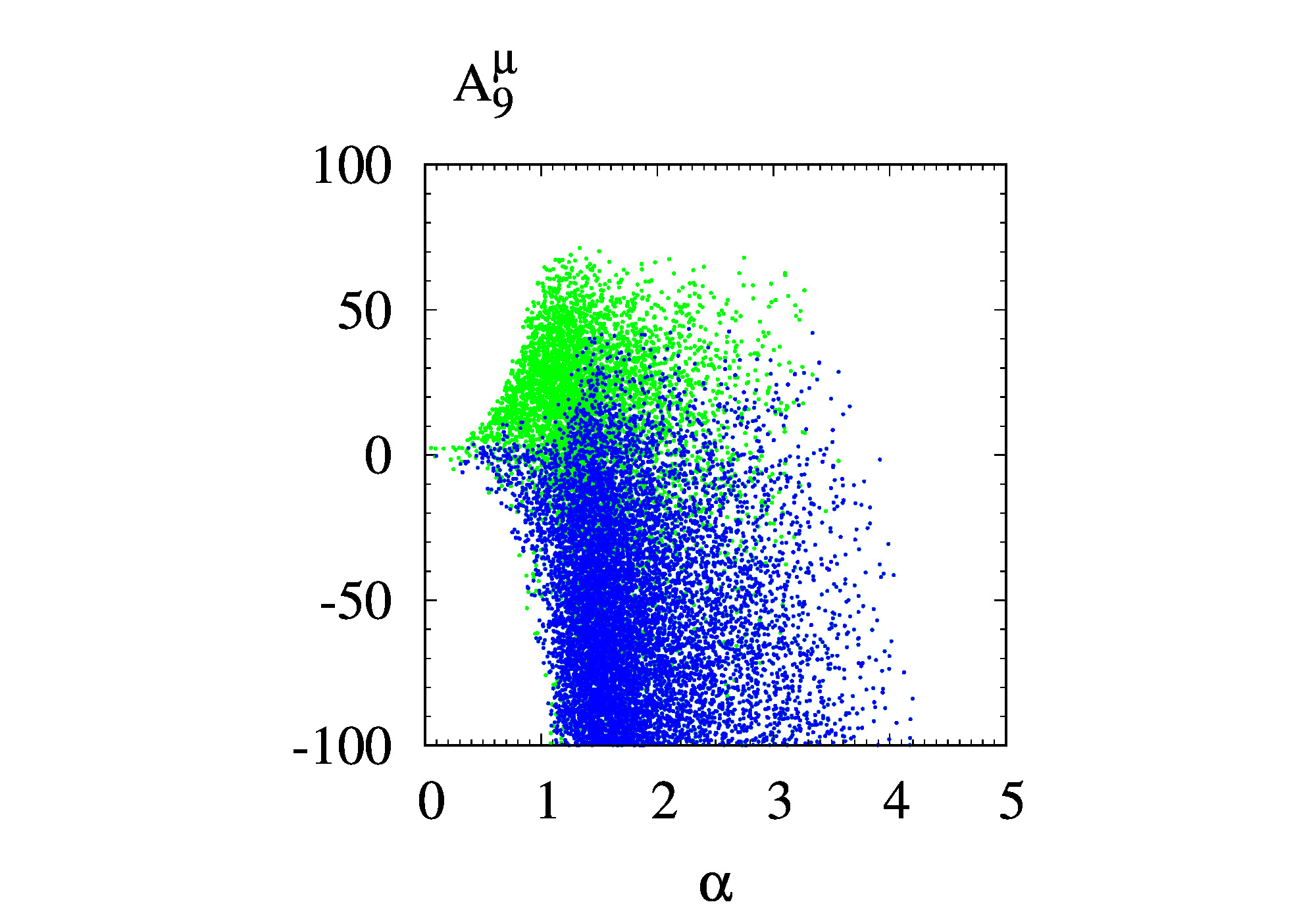
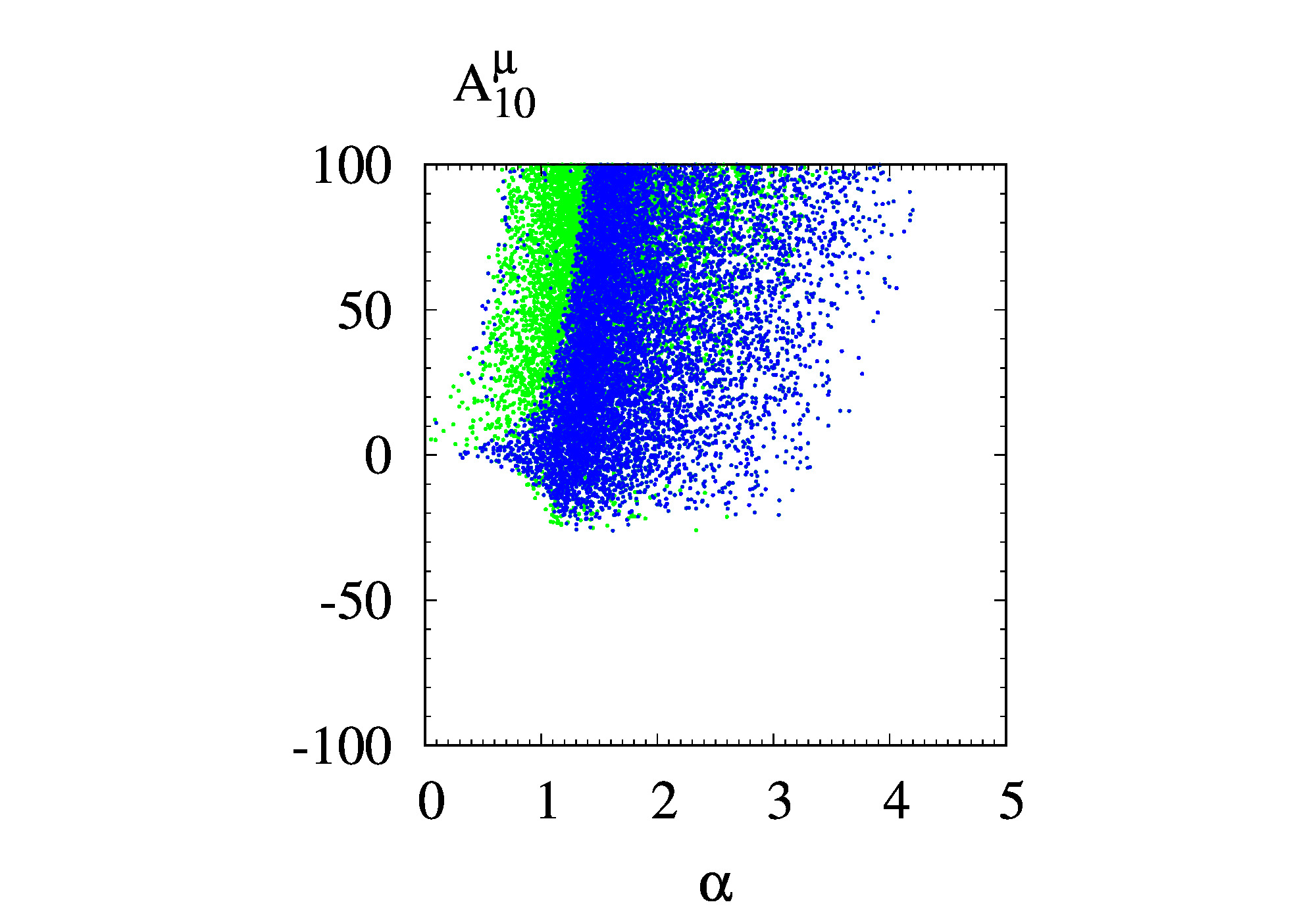
(a)	(b)
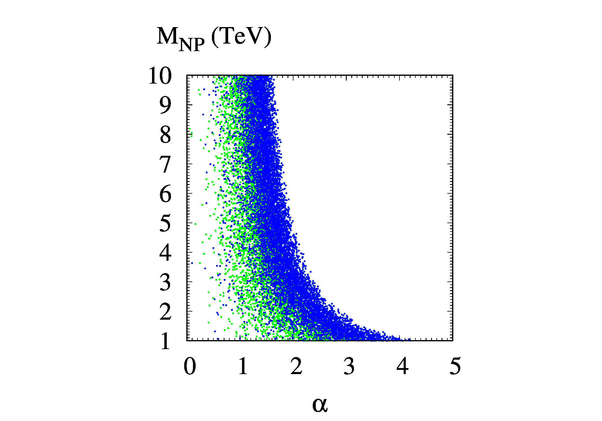
(c)

Figure 1: Allowed regions of (a) $A_{9}^{\mu}$ vs $\alpha$, (b) $A_{10}^{\mu}$ vs $\alpha$, and (c) $M_{\rm NP}$ vs $\alpha$ at the $2\sigma$ level by $R({K^{(*)}})$ (green). Blue dots represent the subregion of the green ones that satisfy the $B_{s}\to\mu^{+}\mu^{-}$ constraint.

Figure 2 shows another aspects of the parameter space. In Figs. 2 (a) and (b) allowed $A_{9,10}^{\mu}$ vs $M_{\rm NP}$ are shown. Here we specify the region where $\alpha=2$ with red dots. Note that $M_{\rm NP}$ is allowed for $\lesssim 5$ TeV for fixed $\alpha=2$.. For larger $M_{\rm NP}$ NP effect gets smaller, which is not good to explain the data. If we extend the parameter window wider, e.g., $|A_{9,10}^{\mu}|\geq 100$, then larger $M_{\rm NP}\gtrsim 5{\rm TeV}$ could be also possible . This is because it is the Wilson coefficients $C_{9,10{\rm NP}}^{\mu}$ that directly affect the values of $R({K^{(*)}})$. For given $C_{9,10{\rm NP}}^{\mu}$, large $|A_{9,10}^{\mu}|$ is compensated by large $M_{\rm NP}$.

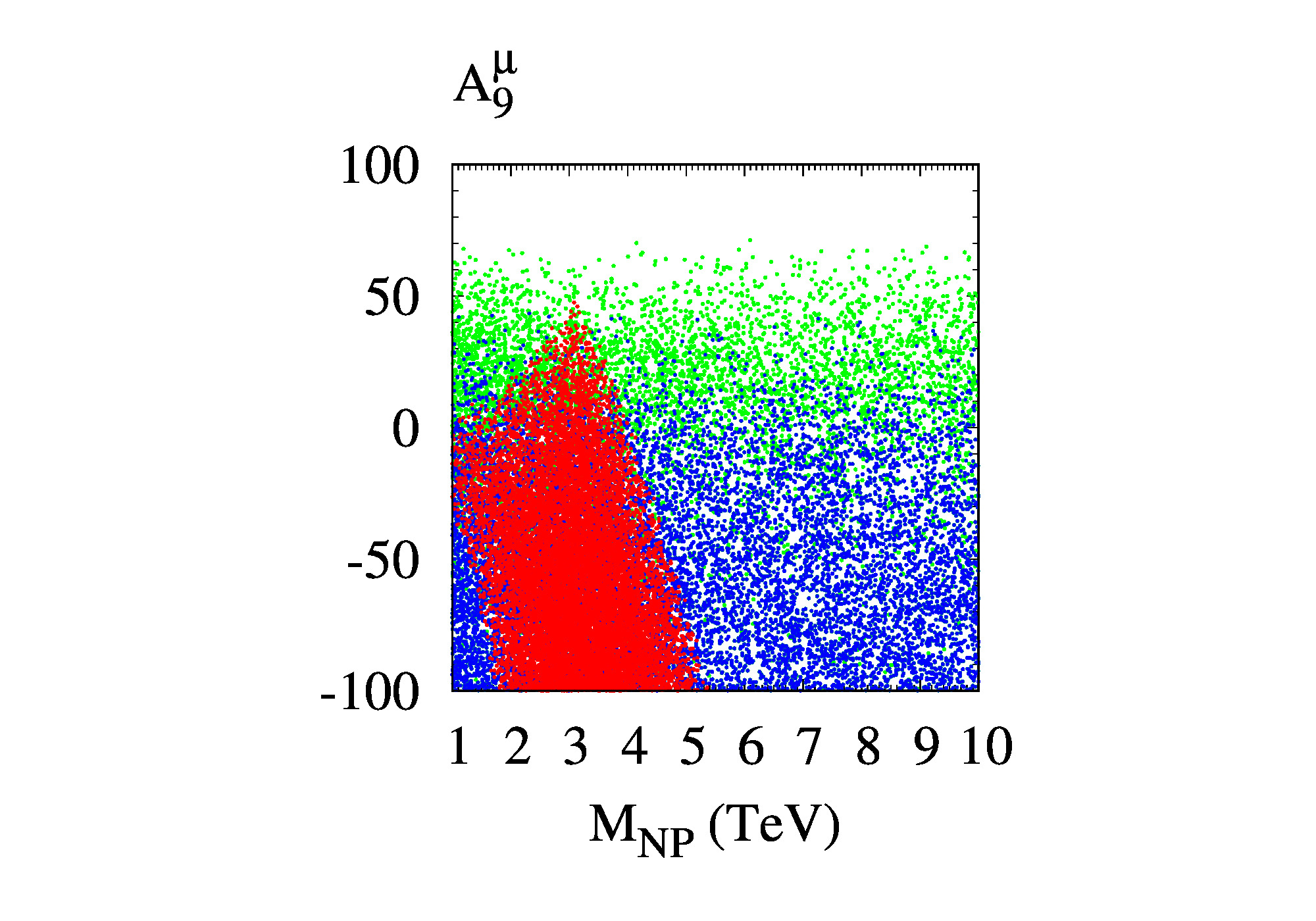
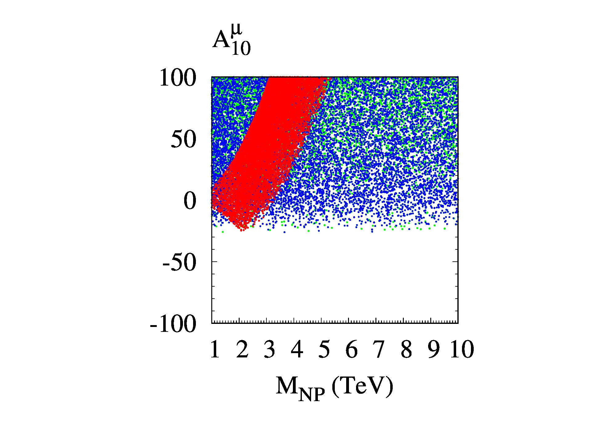
(a)	(b)
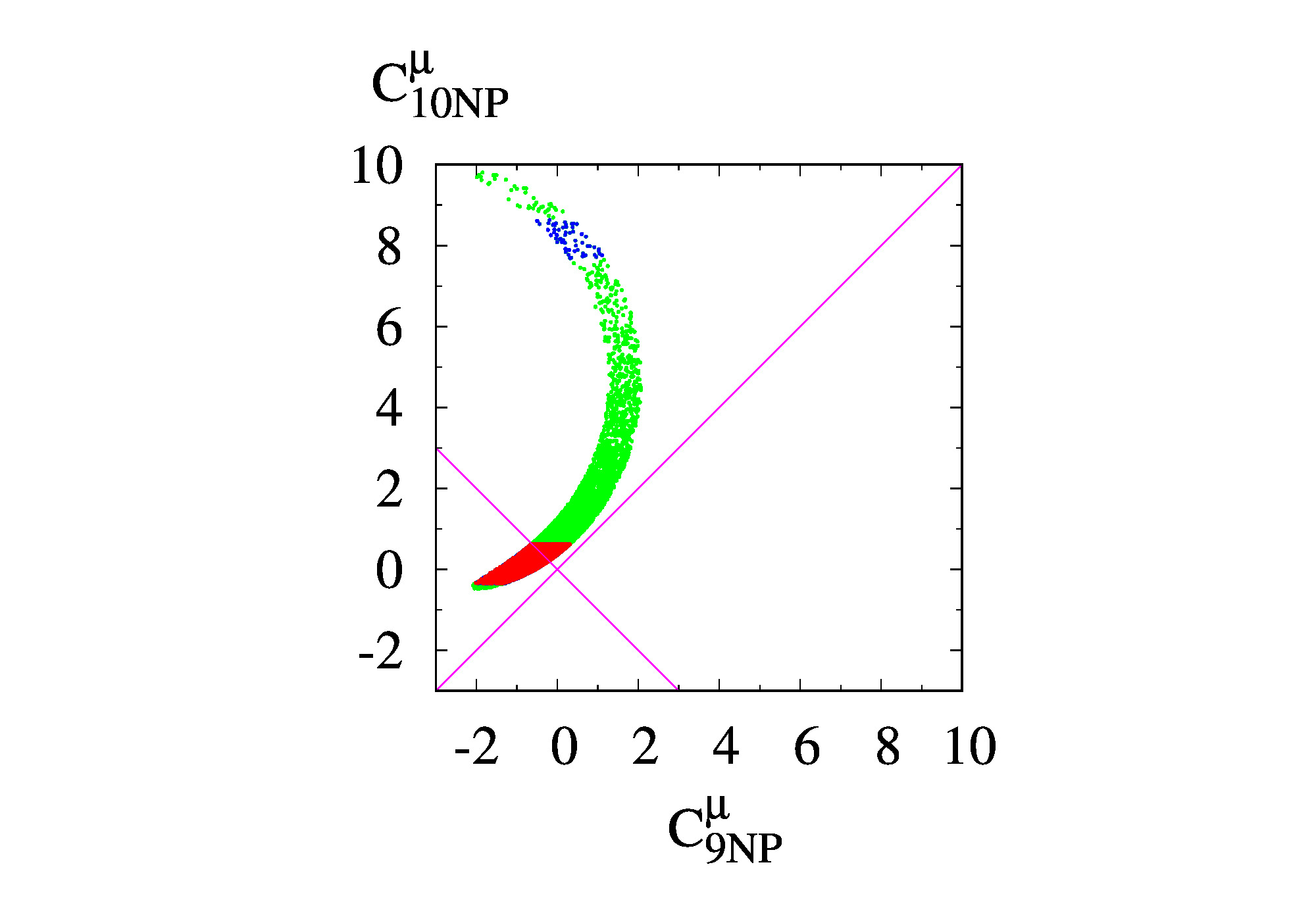
(c)

Figure 2: Allowed regions of (a) $A_{9}^{\mu}$ vs $M_{\rm NP}$, (b) $A_{10}^{\mu}$ vs $M_{\rm NP}$, and (c) $C_{10{\rm NP}}^{\mu}$ vs $C_{9{\rm NP}}^{\mu}$ at the $2\sigma$ level by $R({K^{(*)}})$ (green). Blue dots represent the subregion of the green ones that satisfy the $B_{s}\to\mu^{+}\mu^{-}$ constraint, and red dots for ${B_{s}\to\mu^{+}\mu^{-}}$ and $\alpha=2$. Magenta lines in (c) represent $C_{9{\rm NP}}^{\mu}=\pm C_{10{\rm NP}}^{\mu}$.

One can see in Fig. 2 (b) that when the constraint of ${B_{s}\to\mu^{+}\mu^{-}}$ is imposed $A_{10}^{\mu}$ is mostly positive. The reason is that $C_{10{\rm NP}}^{\mu}/C_{10{\rm SM}}^{\mu}$ favors negative values to fit the experimental data, and $C_{10{\rm SM}}^{\mu}<0$ Buras1303 . The Wilson coefficients $C_{9,10{\rm NP}}^{\mu}$ is presented in Fig. 2 (c). Compared to other Figures like Figs. 1 (a)-(c) and Figs. 2 (a)-(b), $C_{9,10{\rm NP}}^{\mu}$ are significantly constrained by ${B_{s}\to\mu^{+}\mu^{-}}$. Figure 2 (c) also shows that $C_{9{\rm NP}}^{\mu}=-C_{10{\rm NP}}^{\mu}$ is still a good solution to the $R({K^{(*)}})$ puzzle. It should be also noted that the SM ($C_{9{\rm NP}}^{\mu}=C_{10{\rm NP}}^{\mu}=0$) is slightly off of the allowed region at the $2\sigma$ level.

Figure 3 is given for the allowed regions of $A_{10}^{\mu}$ vs $A_{9}^{\mu}$ with respect to $M_{\rm NP}$, and $R({K^{(*)}})$. Comparing Figs. 3 (a) and (b), constraints from ${B_{s}\to\mu^{+}\mu^{-}}$ reduce the allowed region of $A_{10}^{\mu}$ more than that of $A_{9}^{\mu}$. Much of the negative $A_{10}^{\mu}$ region is forbidden by ${B_{s}\to\mu^{+}\mu^{-}}$, as discussed before. And the distribution of $M_{\rm NP}$ is influenced little by ${B_{s}\to\mu^{+}\mu^{-}}$, which is also clear in Fig. 1 (c).

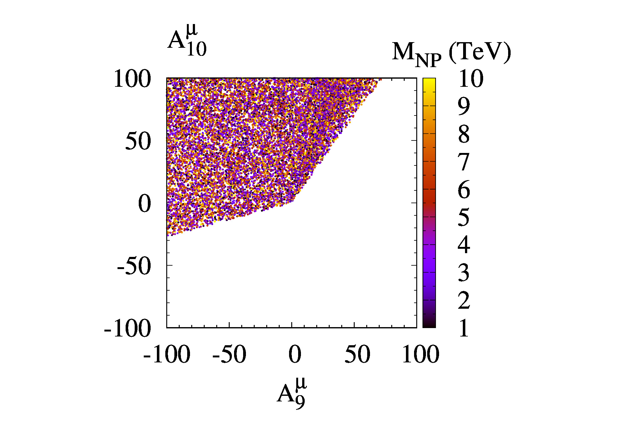
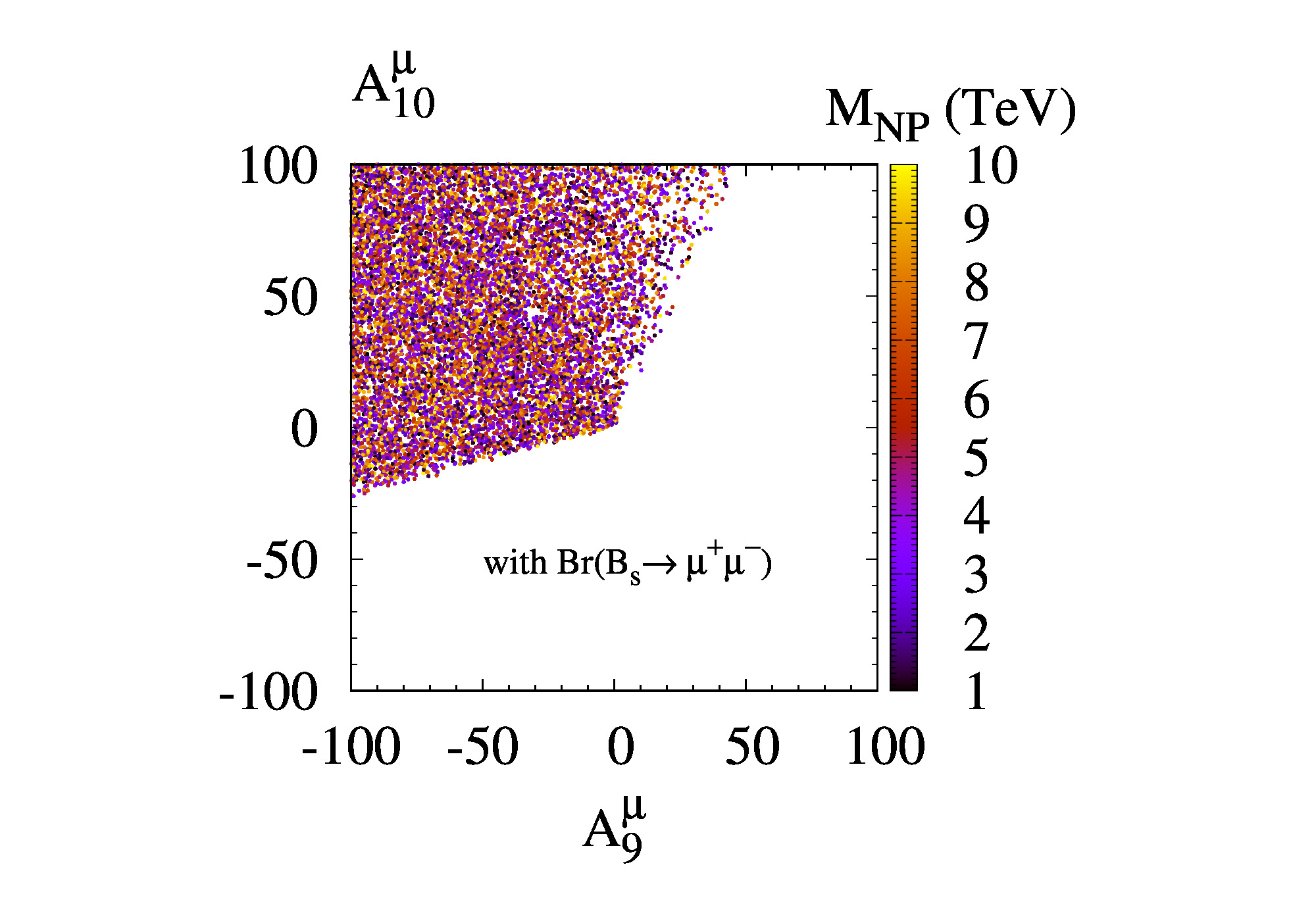
(a)	(b)
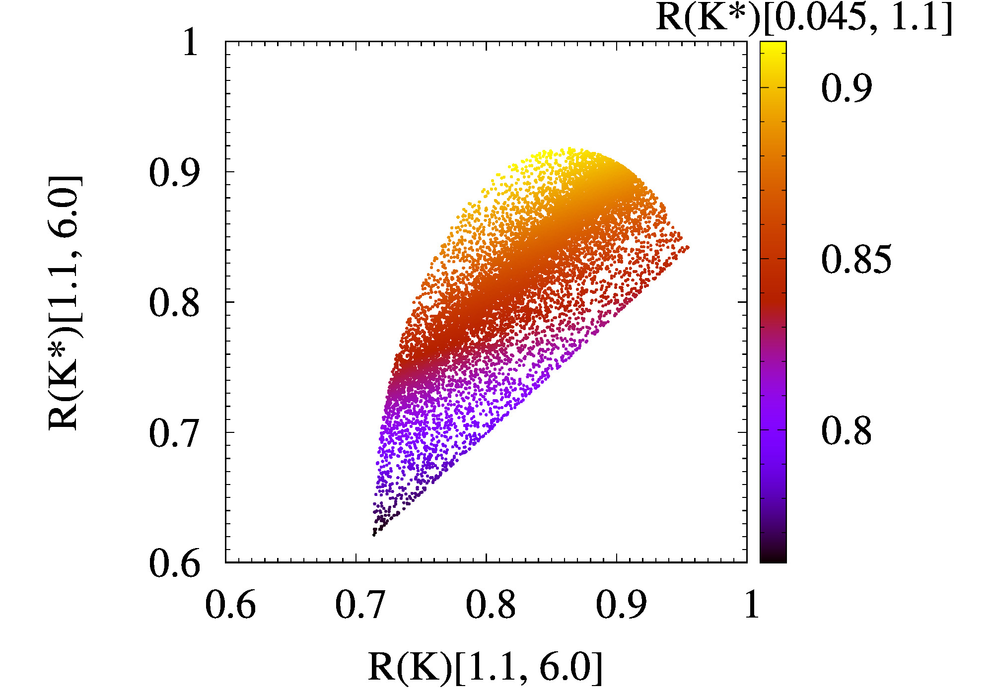
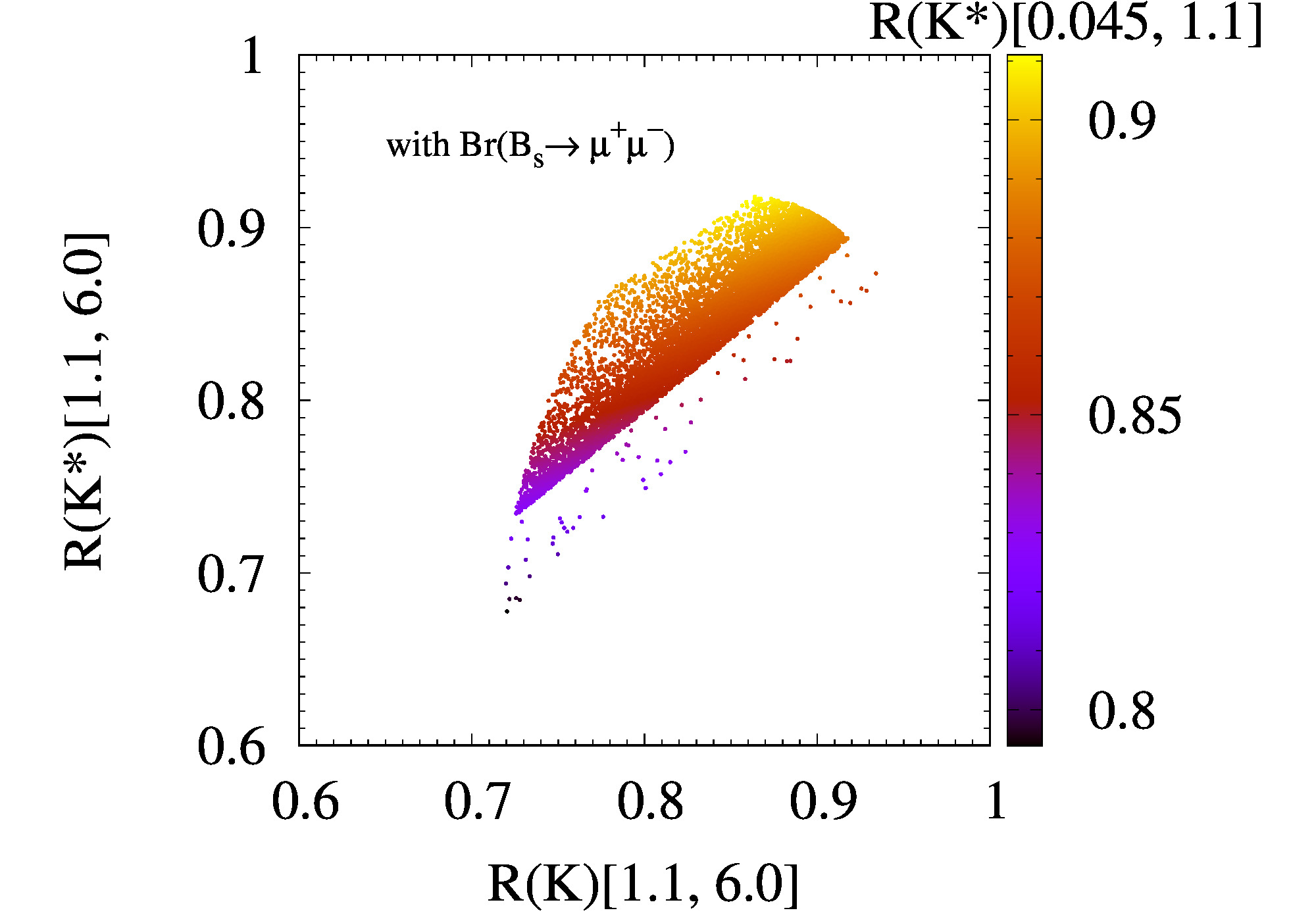
(c)	(d)

Figure 3: Allowed regions of (a) $A_{10}^{\mu}$ vs $A_{9}^{\mu}$ with respect to $M_{\rm NP}$ and (b) the subregion of (a) where ${\rm Br}({B_{s}\to\mu^{+}\mu^{-}})$ is satisfied; (c) $R(K^{*})[1.1,6.0]$ vs $R(K)[1.1,6.0]$ with respect to $R(K^{*})[0.045,1.1]$ and (d) the subregion of (c) where ${\rm Br}({B_{s}\to\mu^{+}\mu^{-}})$ is satisfied, at the $2\sigma$ level with $0\leq\alpha\leq 5$.

As for $R({K^{(*)}})$ in Figs. 3 (c) and (d), parameters that enhance one of $R({K^{(*)}})$s have a tendency to make other $R({K^{(*)}})$s get larger. Figure 3 (d) shows that the constraint from ${B_{s}\to\mu^{+}\mu^{-}}$ picks out the middle band-like region of Fig. 3 (c). In specific models, one should include other constraints like $(g-2)_{\mu}$, $B_{s}$-${\bar{B}}_{s}$ mixing, etc.

Since $\alpha_{\rm best}=1.24$ unparticle-like scenario is favored more than other NP models where $\alpha=2$. But for unparticles the scaling dimensions $d_{S}$ (for scalar) and $d_{V}$ (for vector) are $d_{S}=\alpha/2~{},d_{V}=\alpha/2+1$ , and the unitarity condition puts bounds as $d_{S}\geq 1$ and $d_{V}\geq 3$. If the unitary bound could be alleviated JPL2106 then $d_{V}$ could be $d_{V}\geq 1~{}(\alpha\geq 0)$, so the vector unparticle might be a good candidate. For the case of $\alpha=2$ where real particles are exchanged at the tree level, we found that the minimum $\chi^{2}$ for the LQ model where $-25\leq A_{9,{\rm LQ}}(=-A_{10,{\rm LQ}})\leq-2.5$ and $2\leq M_{\rm NP}\leq 4~{}({\rm TeV})$ Du2104 is $\chi^{2}_{{\rm min},{\rm LQ}}/{\rm d.o.f.}=4.39$. As a comparison for $Z^{\prime}$ model where $-27.2\leq A_{9,Z^{\prime}}(=-A_{10,Z^{\prime}})\leq-3.35$ and $3\leq M_{\rm NP}\leq 6~{}({\rm TeV})$ Davighi2105 , we got $\chi^{2}_{{\rm min},Z^{\prime}}/{\rm d.o.f.}=7.75$. At least for these windows of the model parameters one can say that LQ is better than $Z^{\prime}$ to fit $R({K^{(*)}})$. As for sbottom exchange in SUSY of Altmannshofer2002 with $-30\leq A_{9,{\rm SUSY}}(=-A_{10,{\rm SUSY}})\leq 0$ and $1\leq M_{\rm NP}\leq 5~{}({\rm TeV})$, we found $\chi^{2}_{{\rm min},{\rm SUSY}}/{\rm d.o.f.}=4.30$. The scan window for sbottom exchange is slightly wider than that of LQ or $Z^{\prime}$, which results in better $\chi^{2}$. For other models we could do similar comparisons.

A comment is in order for the form-factor dependence. Current analysis is based on the exponential function for the relevant form factors as in Eq. (11). In JPL2110 , outputs from different kind of form factors which have the pole structure are compared. The result is that general features are quite the same though some details are different. It seems that the form-factor dependence in the numerators of $R({K^{(*)}})$ is cancelled out by the one in the denominators. This kind of cancellation can be found in the hadronic uncertainties in the SM Geng1704 .

Finally, we give comments on the new experimental data from the LHCb LHCb2212_52 ; LHCb2212_53 . Compared to the previous results, the numbers get enhanced close to unity (and to the SM predictions) LHCb2212_53

$$R(K)[{\rm low}~{}q^{2}] = 0.994^{+0.094}_{-0.087}~{},~{}~{}~{}R(K)[{\rm central}~{}q^{2}]=0.949^{+0.048}_{-0.047}~{},$$ (34)

$$R(K^{*})[{\rm low}~{}q^{2}] = 0.927^{+0.099}_{-0.093}~{},~{}~{}~{}R(K^{*})[{\rm central}~{}q^{2}]=1.027^{+0.077}_{-0.073}~{}.$$ (35)

The new data are far away from the previous one and if we include the above data the $\chi^{2}$ fitting would get worse. A preliminary analysis says that when including new data the $\chi^{2}_{\rm min}/{\rm d.o.f.}$ gets larger, $\chi^{2}_{\rm min}/{\rm d.o.f.}=3.05$ as expected. If we discard old data and keep only new data, then it would provide a strong constraint for NP.

IV Conclusions

In conclusion, we performed the $\chi^{2}$ fit to $R({K^{(*)}})$ with a general parametrization of the NP effects for the Wilson coefficients by using the NP scale $M_{\rm NP}$, its power $\alpha$, and the corresponding coefficients $A_{9,10}^{\mu}$. In this framework the constraint from ${B_{s}\to\mu^{+}\mu^{-}}$ is naturally incorporated with $R({K^{(*)}})$. This kind of parametrization for NP includes the leptoquark model, $Z^{\prime}$ model, SUSY, and so on. It is known that the relevant Wilson coefficients of $\sim{\cal O}(1)$ is compatible with the data. Our parametrization makes it easy to produce $\sim{\cal O}(1)$ Wilson coefficients within natural ranges of the parameters. In this analysis we considered the NP effects only in the muon sector. Our results for the Wilson coefficients include the usual solution where $C_{9{\rm NP}}^{\mu}=-C_{10{\rm NP}}^{\mu}$. We found that for the coefficients of $|A_{9,10}^{\mu}|$ up to $\sim{\cal O}(2)$ with $\alpha=2$, the NP scale $M_{\rm NP}$ is restricted to be $M_{\rm NP}\lesssim 5{\rm TeV}$. The upper limit of $M_{\rm NP}$ gets higher for larger $|A_{9,10}^{\mu}|$. Current analysis was based on the exponential function for the form factors of the matrix elements, but it is expected that the form-factor dependence would be weak. Our framework would work as a good starting point for specific models to attack the $R({K^{(*)}})$ puzzle.

References

(1)
R. Aaij et al. [LHCb],
[arXiv:2103.11769 [hep-ex]].
(2)
R. Aaij et al. [LHCb],
JHEP 08 (2017), 055.
(3)
L. S. Geng, B. Grinstein, S. Jäger, S. Y. Li, J. Martin Camalich and R. X. Shi,
[arXiv:2103.12738 [hep-ph]].
(4)
G. Hiller and F. Kruger,
Phys. Rev. D 69 (2004), 074020.
(5)
C. Bobeth, G. Hiller and G. Piranishvili,
JHEP 12 (2007), 040.
(6)
L. S. Geng, B. Grinstein, S. Jäger, J. Martin Camalich, X. L. Ren and R. X. Shi,
Phys. Rev. D 96 (2017) no.9, 093006.
(7)
W. Altmannshofer, P. S. B. Dev, A. Soni and Y. Sui,
Phys. Rev. D 102 (2020) no.1, 015031.
(8)
D. Bardhan, D. Ghosh and D. Sachdeva,
Nucl. Phys. B 986, 116059 (2023).
(9)
G. Hiller and M. Schmaltz,
Phys. Rev. D 90 (2014), 054014.
(10)
I. Doršner, S. Fajfer, A. Greljo, J. F. Kamenik and N. Košnik,
Phys. Rept. 641 (2016), 1-68.
(11)
M. Bauer and M. Neubert,
Phys. Rev. Lett. 116 (2016) no.14, 141802.
(12)
C. H. Chen, T. Nomura and H. Okada,
Phys. Lett. B 774 (2017), 456-464.
(13)
A. Crivellin, D. Müller and T. Ota,
JHEP 09 (2017), 040.
(14)
L. Calibbi, A. Crivellin and T. Li,
Phys. Rev. D 98 (2018) no.11, 115002.
(15)
M. Blanke and A. Crivellin,
Phys. Rev. Lett. 121 (2018) no.1, 011801.
(16)
T. Nomura and H. Okada,
[arXiv:2104.03248 [hep-ph]].
(17)
A. Angelescu, D. Bečirević, D. A. Faroughy, F. Jaffredo and O. Sumensari,
[arXiv:2103.12504 [hep-ph]].
(18)
M. Du, J. Liang, Z. Liu and V. Tran,
[arXiv:2104.05685 [hep-ph]].
(19)
K. Cheung, W. Y. Keung and P. Y. Tseng,
Phys. Rev. D 106, no.1, 015029 (2022).
(20)
A. Crivellin, G. D’Ambrosio and J. Heeck,
Phys. Rev. Lett. 114 (2015), 151801.
(21)
A. Crivellin, G. D’Ambrosio and J. Heeck,
Phys. Rev. D 91 (2015) no.7, 075006.
(22)
C. W. Chiang, X. G. He, J. Tandean and X. B. Yuan,
Phys. Rev. D 96 (2017) no.11, 115022.
(23)
S. F. King,
JHEP 08 (2017), 019.
(24)
R. S. Chivukula, J. Isaacson, K. A. Mohan, D. Sengupta and E. H. Simmons,
Phys. Rev. D 96 (2017) no.7, 075012.
(25)
J. Y. Cen, Y. Cheng, X. G. He and J. Sun,
[arXiv:2104.05006 [hep-ph]].
(26)
J. Davighi,
[arXiv:2105.06918 [hep-ph]].
(27)
Q. Y. Hu, X. Q. Li and Y. D. Yang,
Eur. Phys. J. C 77 (2017) no.3, 190.
(28)
A. Crivellin, D. Müller and C. Wiegand,
JHEP 06 (2019), 119.
(29)
L. Delle Rose, S. Khalil, S. J. D. King and S. Moretti,
Phys. Rev. D 101 (2020) no.11, 115009.
(30)
J. P. Lee,
[arXiv:2106.12795 [hep-ph]].
(31)
J. P. Lee,
J. Korean Phys. Soc. 80, no.1, 13-19 (2022).
(32)
R. Alonso, B. Grinstein and J. Martin Camalich,
Phys. Rev. Lett. 113 (2014), 241802.
(33)
L. S. Geng, B. Grinstein, S. Jäger, J. Martin Camalich, X. L. Ren and R. X. Shi,
Phys. Rev. D 96 (2017) no.9, 093006.
(34)
A. Ali, P. Ball, L. T. Handoko and G. Hiller,
Phys. Rev. D 61 (2000), 074024.
(35)
Q. Chang, X. Q. Li and Y. D. Yang,
JHEP 04, 052 (2010).
(36)
H. Georgi,
Phys. Rev. Lett. 98, 221601 (2007);
Phys. Lett. B 650, 275 (2007).
(37)
D. Becirevic, N. Kosnik, F. Mescia and E. Schneider,
Phys. Rev. D 86, 034034 (2012).
(38)
M. Beneke, C. Bobeth and R. Szafron,
JHEP 10 (2019), 232.
(39)
R. L. Workman et al. [Particle Data Group],
PTEP 2022, 083C01 (2022).
(40)
CMS,
“Measurement of decay properties and search for the decay in proton-proton collisions at ,”
CMS-PAS-BPH-21-006.
(41)
A. J. Buras, R. Fleischer, J. Girrbach and R. Knegjens,
JHEP 07, 077 (2013).
(42)
LHCb,
“Test of lepton universality in decays,”
arXiv:2212.09152 [hep-ex].
(43)
LHCb,
“Measurement of lepton universality parameters in and decays,”
arXiv:2212.09153 [hep-ex].