Modeling, Quantifying, and Predicting Subjectivity of Image Aesthetics

Abstract

Assessing image aesthetics is a challenging computer vision task. One reason is that aesthetic preference is highly subjective and may vary significantly among people for certain images. Thus, it is important to properly model and quantify such subjectivity, but there has not been much effort to resolve this issue. In this paper, we propose a novel unified probabilistic framework that can model and quantify subjective aesthetic preference based on the subjective logic. In this framework, the rating distribution is modeled as a beta distribution, from which the probabilities of being definitely pleasing, being definitely unpleasing, and being uncertain can be obtained. We use the probability of being uncertain to define an intuitive metric of subjectivity. Furthermore, we present a method to learn deep neural networks for prediction of image aesthetics, which is shown to be effective in improving the performance of subjectivity prediction via experiments. We also present an application scenario where the framework is beneficial for aesthetics-based image recommendation.

1 Introduction

Image aesthetic assessment is to automatically evaluate the image in the aesthetic viewpoint, i.e., how aesthetically pleasing to human viewers an image will be. It is a challenging computer vision task since it requires to imitate high-level aesthetic perception of humans, but it can be useful in many applications including image search and retrieval, recommender systems, image enhancement, etc.

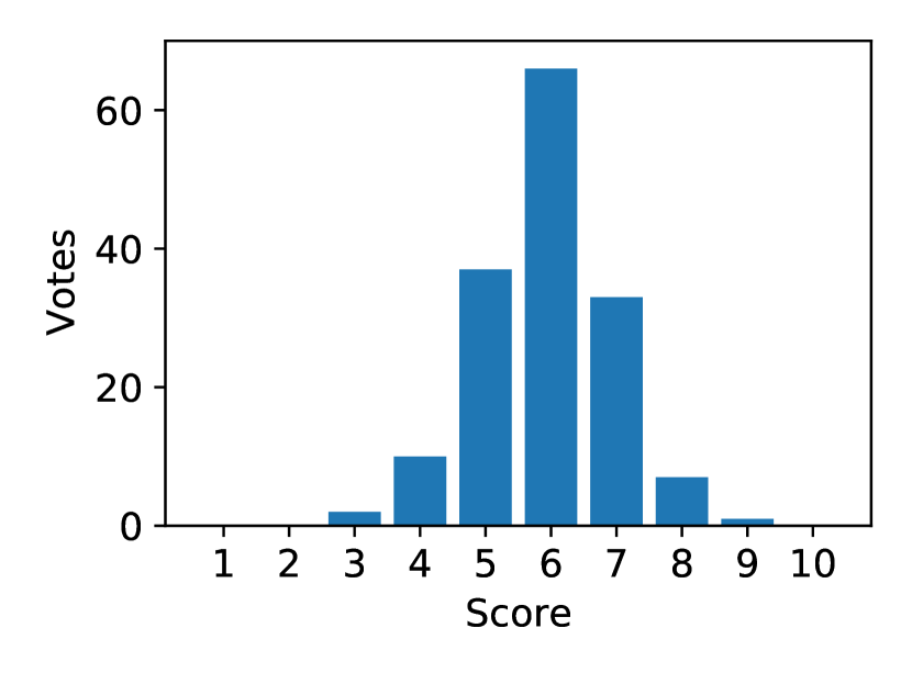
(a) Image having low subjectivity

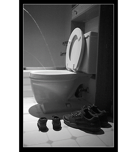
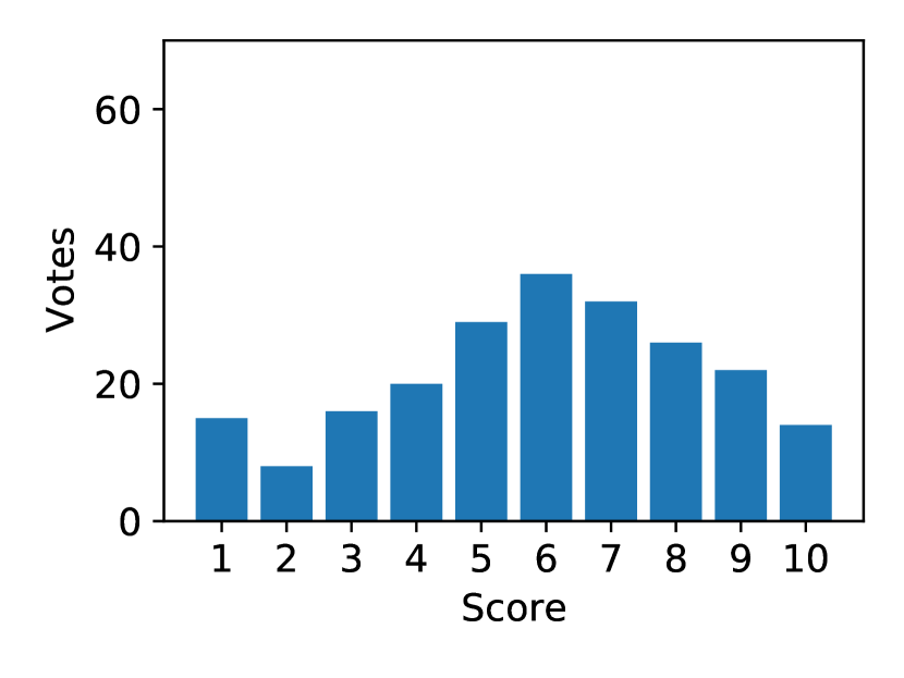
(b) Image having high subjectivity

Figure 2: Example images and their histograms of the rating scores given by raters. The two images have similar mean rating scores (about 5.92) but different degrees of subjectivity.

In order to obtain the aesthetic ground truth of an image, it is usual to ask a group of raters to provide aesthetic scores for the image. In the binary classification task, the image is considered as aesthetically pleasing if the mean score is higher than a threshold, and as unpleasing otherwise. It is also possible to set a regression task where the mean rating score is predicted. However, these tasks do not consider the diversity in the raters’ opinions. In Fig. 2, two example images and their histograms of the rating scores from raters are shown, which are from the AVA dataset [1]. The two images have similar mean scores (about 5.92), so that they have the same target mean rating score for mean rating regression and the same class label for binary classification. However, these do not capture the different levels of diversity in the raters’ opinions between the two cases. While the distribution of ratings in Fig. 2(a) is concentrated around the mean score, that in Fig. 2(b) is spread widely over the whole score range. Thus, in the case of Fig. 2(b), the results of the mean rating regression and binary classification may be disagreed by a significant proportion of users.

Therefore, it is necessary to consider subjectivity in aesthetic assessment. However, only a limited number of existing studies have dealt with the issue of subjectivity. In particular, the problem of quantifying the level of subjectivity still remains unanswered. A straightforward way is to compute the standard deviation (STD) (or variance) of the rating scores. However, it has an issue in terms of interpretability because it does not have an upper limit and the meaning of its scale is unclear. Similar metrics exist, such as mean absolute deviation around median [2], which suffer from the same problem.

In this paper, we propose a novel unified probabilistic framework for modeling and quantifying the subjectivity of image aesthetics based on the subjective logic [3]. In this framework, the rating distribution of an image is modeled as a beta distribution, from which the probabilities of being definitely pleasing, being definitely unpleasing, and being uncertain can be obtained simultaneously. In particular, the probability of being uncertain defines an intuitive metric of subjectivity, named aesthetic uncertainty. Unlike the existing subjectivity metrics, it is a probability measure, which can be easily interpreted. Furthermore, we present a method to train deep neural networks for effective prediction of the subjectivity metrics. We also present an application scenario where the framework is beneficial for aesthetics-based image recommendation.

2 Related work

2.1 Image aesthetic assessment

In literature, three tasks have been mainly considered for automatic aesthetic assessment of images: binary classification, mean score regression, and rating distribution prediction. The binary classification task distinguishing pleasing vs. unpleasing images has been considered most popularly. There exist several methods, from those using handcrafted features [4, 5, 6] to deep learning-based methods [7, 8, 9, 10]. To obtain more informative results than binary class information, the mean rating regression task has been addressed [11, 12, 13]. Prediction of the whole score distribution has been also considered [14, 15, 16, 17], which is the most challenging but has potential to provide the most comprehensive information regarding the aesthetic characteristics of the given image. In this paper, we consider all these tasks and also the subjectivity regression task.

2.2 Subjectivity of image aesthetics

Subjectivity is a clearly distinguished issue in image aesthetics compared to other image-based problems such as object classification. While the class of an object in an image can be objectively determined, subjective judgement is involved in image aesthetics, and thus an image preferred by certain viewers is not necessarily pleasing to some other viewers. Park et al. [18] modeled the human aesthetic evaluation process by a dynamic system and showed that the response time for aesthetic evaluation of an image is related to the subjectivity level of the image in terms of STD. Kim et al. [19] analyzed the relationship between subjectivity (expressed by STD) and user comments, which showed that several factors such as unusualness and coexistence of aesthetic merits and demerits are involved in determining the level of subjectivity of an image. There also exist studies suggesting personalized image aesthetic assessment techniques that reflect the information of a specific user [20, 21, 22, 12, 23, 24, 25].

The rating distribution itself can give the information regarding subjectivity (as in Fig. 2) but only implicitly [2]. Therefore, there is a need to explicitly quantify subjectivity as a scalar value. However, there is not much progress in this research direction. STD has been mostly used [14, 26]. Kang et al. [2] defined additional subjectivity metrics including the mean absolute deviation around the median (MAD), distance to uniform distribution (DUD), and distance from the maximum entropy distribution (MED). However, all these metrics have a limitation in interpretability because they have neither upper limits nor interpretable scales (except 0). Our work addresses this issue and proposes an intuitive metric of subjectivity.

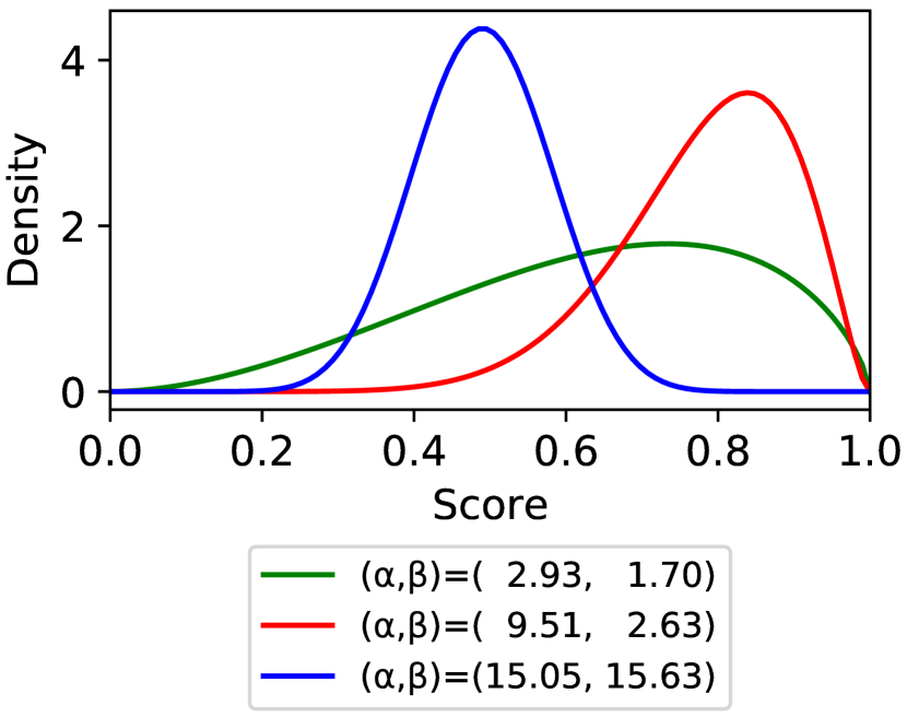
(a) Beta distribution

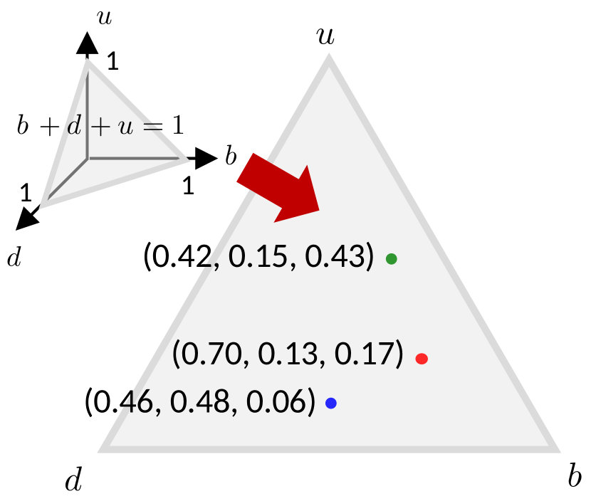
(b) Triple $(b,d,u)$

Figure 3: Image aesthetics via the subjectivity modeling. The fitted beta distributions and the corresponding triples of $(b,d,u)$ on the equilateral triangle are shown.

3 Proposed method for subjectivity modeling

The proposed unified framework is based on the subjective logic [3]. The subjective logic is a probabilistic reasoning for modeling subjective opinions involving uncertainty. An aesthetic rating chosen from a range of scores (e.g., 1 to 10) is a multinomial opinion. However, if the rating scale is normalized between 0 and 1, the rating can be considered as a binomial opinion indicating the subjective belief about aesthetic pleasingness of the image. Then, this binomial opinion is represented by three components [3]: $b$ (belief mass), $d$ (disbelief mass), and $u$ (uncertainty mass), which correspond to the probabilities of being definitely pleasing, being definitely unpleasing, and being uncertain, respectively. These components have values between 0 and 1, and satisfy $b+d+u=1$. As a result, the aesthetics of an image can be represented as a point on a equilateral triangle as shown in Fig. 3(b).

The binomial opinion can be modeled by a beta distribution whose probability density function (PDF) is given by

$$f(x;\alpha,\beta)=\frac{1}{B(\alpha,\beta)}x^{\alpha-1}(1-x)^{\beta-1},$$ (1)

where 0 $\leq$ $x$ $\leq$ 1, $\alpha$ and $\beta$ are shape parameters, and $B(\alpha,\beta)$ is a normalization constant ensuring $\int_{0}^{1}f(x;\alpha,\beta)dx=1$. When the rating distribution of an image is given, a beta distribution is fitted to the distribution by finding the optimal values of $\alpha$ and $\beta$ that minimize the difference (e.g., earth movers’ distance (EMD)) between the given and fitted distributions.

Finally, the three probabilities ($b$, $d$, and $u$) can be obtained from the fitted values of $\alpha$ and $\beta$ as follows [3]:

$$b= \frac{\alpha-1}{\alpha+\beta},$$ (2)

$$d= \frac{\beta-1}{\alpha+\beta},$$

$$u= \frac{2}{\alpha+\beta}.$$

Fig. 3 shows examples of fitted beta distributions and their representations in the equilateral triangle of $b$, $d$, and $u$. The image corresponding to the red-colored distribution in Fig. 3(a) would be considered as aesthetically pleasing by most people, which is reflected in the large value of $b$ and the small value of $u$ in Fig. 3(b). The blue-colored case in Fig. 3(a) is judged to have an intermediate level of aesthetics without much disagreement among people, which is represented by the small value of $u$ and the similar values of $b$ and $d$ in Fig. 3(b). The green-colored case would be classified as pleasing if binary classification is performed, but it involves high subjectivity; thus, $u$ appears to be large while $b>d$.

The beta distribution is unimodal, while an original rating distribution may be multimodal. An example case is shown in Fig. 4(b), along with the fitted beta distribution. For the images in the AVA dataset [1] used in our experiments, we conduct the dip test of unimodality [27] and find that 94.56% of the images have unimodal distributions, whereas only 5.14% and 0.30% are bimodal and trimodal, respectively. Note that some of the multimodal distributions may be due to noise in the ratings, which can be reduced by the unimodal modeling. Thus, we can say that fitting to beta distributions is reasonable.

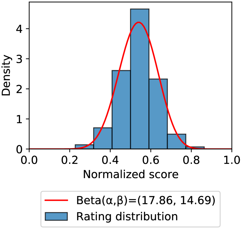
(a) Unimodal

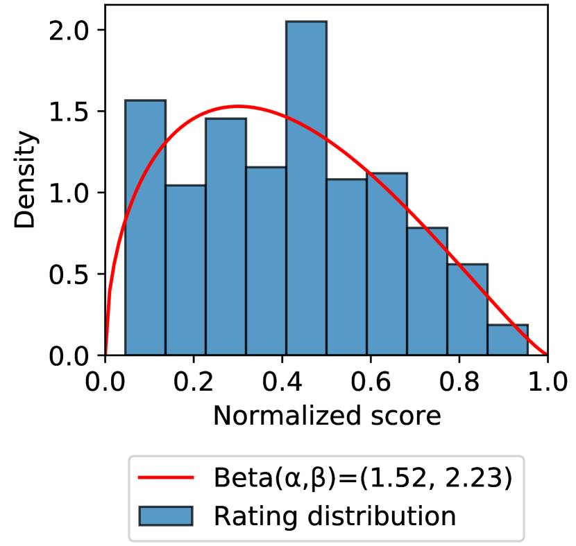
(b) Multimodal

Figure 4: Examples of unimodal and multimodal aesthetic rating distributions (after score normalization) and the fitted beta distributions.

3.1 Aesthetic uncertainty (AesU)

We define a new metric quantifying the level of subjectivity, called aesthetic subjectivity (AesU), by $u$ obtained from the subjectivity modeling. It has several advantages compared to the existing metrics. Since AesU is a probability within [0, 1], one can intuitively grasp the level of subjectivity, whereas the scales of the existing metrics are not well defined and thus not sufficiently intuitive. In addition, AesU can be interpreted together with the other two probabilities ($b$ and $u$) as discussed in Fig. 3(b), which is difficult with the mean and STD (or, MAD, DUD, MED) of ratings.

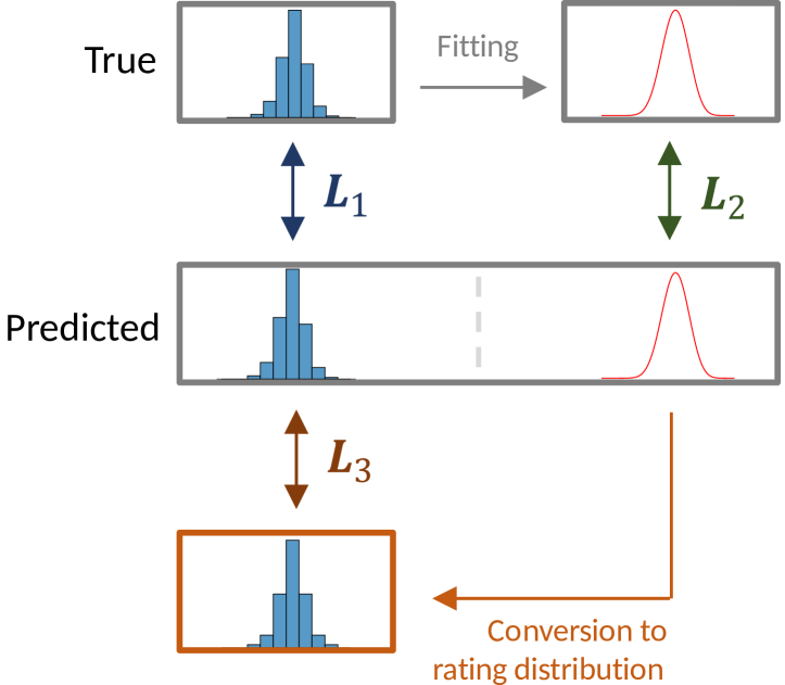
Figure 5: Schematic diagram of the losses used in the proposed simultaneous learning. The learned model predicts both the rating distribution and the shape parameters of the fitted beta distribution, from which $L_{1}$ and $L_{2}$ are computed, respectively. The predicted shape parameters are used for conversion to a rating distribution, for which $L_{3}$ is computed. The total loss is a weighted sum of $L_{1}$, $L_{2}$, and $L_{3}$.

Approach	Backbone	Performance measure	STD	MAD	MED	DUD	AesU
Conventional (rating distribution learning)	VGG16	PLCC ↑	0.2314	0.2041	0.3065	0.3188	0.2231
	ResNet50		0.2653	0.2539	0.3334	0.3627	0.2483
	ConvNeXT-T		0.2930	0.2898	0.3643	0.3900	0.2750
	HLAGCN		0.2399	0.1896	0.3347	0.3784	0.1638
Proposed (simultaneous learning)	VGG16		0.2795	0.2727	0.3256	0.3320	0.2731
	ResNet50		0.3148	0.3056	0.3665	0.3838	0.3120
	ConvNeXT-T		0.3295	0.3338	0.3899	0.4105	0.3331
	HLAGCN		0.3318	0.3194	0.3854	0.3918	0.3265
Conventional (rating distribution learning)	VGG16	SROCC ↑	0.2283	0.2031	0.2925	0.2736	0.2311
	ResNet50		0.2582	0.2523	0.3148	0.3175	0.2527
	ConvNeXT-T		0.2849	0.2810	0.3419	0.3425	0.2764
	HLAGCN		0.2829	0.2737	0.3402	0.3393	0.2745
Proposed (simultaneous learning)	VGG16		0.2717	0.2701	0.3118	0.2939	0.2762
	ResNet50		0.3029	0.2994	0.3451	0.3400	0.3081
	ConvNeXT-T		0.3164	0.3261	0.3639	0.3601	0.3277
	HLAGCN		0.3210	0.3136	0.3647	0.3519	0.3241
Conventional (rating distribution learning)	VGG16	MAE ↓	0.1551	0.1531	0.0537	0.0638	0.0345
	ResNet50		0.1513	0.1492	0.0533	0.0609	0.0343
	ConvNeXT-T		0.1544	0.1499	0.0526	0.0595	0.0343
	HLAGCN		0.1631	0.1555	0.0536	0.0622	0.0351
Proposed (simultaneous learning)	VGG16		0.1565	0.1462	0.0533	0.0606	0.0340
	ResNet50		0.1608	0.1439	0.0526	0.0565	0.0336
	ConvNeXT-T		0.1550	0.1431	0.0520	0.0572	0.0333
	HLAGCN		0.1544	0.1436	0.0520	0.0575	0.0333

TABLE I: Results of subjectivity regression. The best and the second best cases are marked with bold faces and underlines, respectively.

4 Predicting image aesthetics

Based on our aesthetic modeling framework, we propose a method to train neural networks for prediction of image aesthetics, called simultaneous learning. We aim to obtain the rating distribution from a trained neural network, so that we can perform any of the binary classification of the mean rating, mean rating regression, subjectivity regression, and rating distribution prediction. For this, it is sufficient to make the neural network predict $\alpha$ and $\beta$ of the fitted beta distribution. Our preliminary experiment showed that this approach improves the performance of subjectivity regression compared to the conventional approach where the rating distribution is predicted, but the performance of the other tasks is lowered instead.

To solve this problem, we design the neural network model so as to predict both the rating distribution and the shape parameters of the fitted beta distribution. For training of the model, we formulate three losses, $L_{1}$, $L_{2}$, and $L_{3}$ (Fig. 5). First, $L_{1}$ is calculated between the ground truth rating distribution ($R_{T}$) and the predicted distribution ($R_{P}$) in terms of EMD, i.e.,

$$L_{1}=\textrm{EMD}(R_{P},R_{T}).$$ (3)

Second, $L_{2}$ is the root mean squared log error (RMSLE) between the ground truth shape parameters (i.e., the shape parameters of the beta distribution fitted to the ground truth rating distribution) ($B_{T}$) and the predicted shape parameters ($B_{P}$):

$$L_{2}=\textrm{RMSLE}(B_{P},B_{T}).$$ (4)

Here, RMSLE is used instead of mean squared error (MSE) or root mean squared error (RMSE) in order to effectively handle the shape parameters that become larger by orders of magnitude occasionally for some images. Third, the predicted shape parameters $B_{P}$ are used to build a rating distribution, which is compared to the predicted rating distribution $R_{P}$:

$$L_{3}=\textrm{EMD}(R_{P},B2R(B_{P})),$$ (5)

where $B2R(B_{P})$ represents the process of converting $B_{P}$ to a rating distribution. This loss reduces the discrepancy between the two sets of model outputs, i.e., the predicted distribution and the beta distribution described by the predicted shape parameters. Finally, the total loss for our simultaneous learning is given by a weighted sum of the three losses, i.e.,

$$L=w_{1}\times L_{1}+w_{2}\times w_{b}\times L_{2}+w_{3}\times L_{3},$$ (6)

where $w_{1}$, $w_{2}$, and $w_{3}$ are the weights for the three losses, respectively, with $w_{1}+w_{2}+w_{3}=1$, and $w_{b}$ is used to compensate for the different scales of EMD and RMSLE.

5 Experiments

5.1 Dataset

We use the AVA dataset [1]. It contains photos and their aesthetic ratings from challenges of DPChallenge. The dataset is composed of 256,000 images. 236,000 images are for training and 20,000 are for test.

5.2 Backbone models

We use popular generic CNN models and a latest image aesthetic assessment model as backbone models for our experiments. The former includes VGG16 [28], ResNet-50 [29], and ConvNeXT-T [30], and the latter corresponds to the hierarchical layout-aware graph convolutional network (HLAGCN) [17]. HLAGCN models the complex relations among interesting regions in the input image using a graph convolutional network.

5.3 Approaches

In the proposed method using the simultaneous learning, a model produces 12 output values (ten for a rating distribution and two for the shape parameters of a beta distribution). For comparison, we employ the conventional approach that predicts only the rating distribution [14, 15, 16, 17].

Approach	Backbone	Binary classification	Mean rating			Distribution
		Accuracy ↑	PLCC ↑	SROCC ↑	MAE ↓	EMD ↓	KLD ↓
Conventional (rating distribution learning)	VGG16	0.7818	0.6632	0.6582	0.447	0.0484	0.0936
	ResNet50	0.7936	0.697	0.6931	0.4282	0.0465	0.0885
	ConvNeXT-T	0.7942	0.7225	0.7207	0.4196	0.0456	0.0841
	HLAGCN	0.7965	0.7031	0.7104	0.4163	0.0459	0.0825
Proposed (simultaneous learning)	VGG16	0.7757	0.6513	0.6443	0.4536	0.0497	0.1044
	ResNet50	0.7933	0.6931	0.6905	0.425	0.0468	0.0963
	ConvNeXT-T	0.7957	0.7156	0.7110	0.4151	0.0462	0.0891
	HLAGCN	0.7942	0.7077	0.7054	0.4158	0.0458	0.0876

TABLE II: Results of binary classification, mean rating regression, and rating distribution prediction. The best and the second best cases are marked with bold faces and underlines, respectively.

5.4 Performance measures

We consider various tasks of image aesthetic assessment, and use appropriate performance measures for each task by following the previous studies [14, 2].

Our simultaneous learning method produces both a predicted rating distribution and a predicted beta distribution (in the form of its shape parameters). Thus, both can be used to measure the performance of the tasks. In our experiments, the predicted rating distribution is used for binary classification, mean rating regression, and rating distribution prediction. For subjectivity regression, the predicted subjectivity metrics are computed from the predicted beta distribution, which yields better performance. The predicted AesU is obtained directly from the predicted shape parameters using Eq. (2). In the case of the conventional approach predicting only the rating distribution, the existing subjectivity metrics are computed using the predicted rating distribution and AesU is obtained after fitting to a beta distribution.

For the binary classification task, the classification accuracy is used. The threshold of the two classes is set to a score of 5 in the scale of 1 to 10 as in [7, 8, 9, 10]. The performance of mean rating regression is measured in terms of mean absolute error (MAE), Pearson linear correlation coefficient (PLCC), and Spearman rank-order correlation coefficient (SROCC) between the ground truth mean ratings and the predicted mean ratings. The same measures are also used for the subjectivity regression task. For distribution prediction, we use EMD and the Kullback-Leibler divergence (KLD) between the ground truth and predicted distributions.

5.5 Implementation details

All experiments are conducted on a PC that has AMD Ryzen 5 5600x CPU, 128GB of RAM, NVIDIA Geforce RTX 3090 24GB GPU, and Microsoft Windows 10. We use Python 3.9.7, PyTorch 1.10.1, CUDA 11.3, and cuDNN 8.0.

We divide the training dataset further into 223,000 training images and 13,000 validation images. The images are resized to $256\times 256$ ($336\times 336$ for HLAGCN) and randomly cropped to $224\times 224$ ($300\times 300$ for HLAGCN). and a random horizontal flip is applied for data augmentations.

In the simultaneous learning, we set $w_{1}=0.4$, $w_{2}=0.5$, and $w_{3}=0.1$, indicating the relative importance of the three losses, and $w_{b}=0.2$.

To train the models, we use the SGD optimization with a batch size of 48, a Nesterov momentum paramenter of 0.9 and a weight decay parameter of $5\times 10^{-4}$. The learning rate is initially set to $5\times 10^{-3}$ and reduced by 5% every 10 epochs. The models are trained for 100 epochs, but if the validation loss does not decrease for 10 epochs, the learning is stopped.

5.6 Results

Table I shows the results of the subjectivity regression task for STD, MAD, MED, DUD, and AesU. The proposed simultaneous learning approach shows improved performance compared to the conventional approach in all cases except that the proposed approach yields the second best performance in the case of STD with MAE. When the backbone models are compared, ConvNeXT-T performs the best, and HLAGCN also performs similarly well. For ConvNeXT-T, the improvement by the proposed approach over the conventional one is about 5% on average, with the maximum improvement by about 21% for AesU in terms of PLCC. These results demonstrate that the proposed simultaneous learning approach using the three losses is effective to learn the subjectivity of image aesthetics. In particular, the proposed subjectivity modeling plays a key role by reducing the noise in the raw rating distribution.

Table II summarizes the results of the other tasks, i.e., binary classification, mean rating regression, and rating distribution prediction. The proposed approach shows slightly lowered performance than the conventional approach but only marginally. The performance decrease by the proposed approach for ConvNeXT-T is only 1.4% on average. Note that this performance decrease is because we tune our approach to maximize the performance of the subjectivity regression task.

Approach	Binary classif.	Mean rating		Dist.	Subjectivity
					STD		MAD		MED		DUD		AesU
	Accuracy	LCC	MAE	EMD	LCC	MAE	LCC	MAE	LCC	MAE	LCC	MAE	LCC	MAE
Rating	0.794	0.723	0.419	0.046	0.293	0.154	0.290	0.150	0.364	0.053	0.390	0.060	0.275	0.034
Beta	0.782	0.682	0.439	0.050	0.339	0.152	0.332	0.144	0.383	0.052	0.377	0.060	0.336	0.033
Both	0.796	0.716	0.415	0.046	0.330	0.155	0.334	0.143	0.390	0.052	0.411	0.057	0.333	0.033

TABLE III: Comparison of the cases where the neural network models output either a predicted rating distribution or a predicted beta distribution (in the form of shape parameters), or both (proposed simultaneous learning). The best and the second best cases are marked with bold faces and underlines, respectively.

Fitting	Binary classif.	Mean rating		Dist.	Subjectivity
					STD		MAD		MED		DUD		AesU
	Accuracy	LCC	MAE	EMD	LCC	MAE	LCC	MAE	LCC	MAE	LCC	MAE	LCC	MAE
w/	0.796	0.716	0.415	0.046	0.330	0.155	0.334	0.143	0.390	0.052	0.411	0.057	0.333	0.033
w/o	0.797	0.712	0.415	0.046	0.283	0.163	0.277	0.145	0.352	0.053	0.403	0.056	0.288	0.034

TABLE IV: Comparison of the two ways measuring $L_{2}$ (without or with fitting to beta distributions) in our simultaneous learning method. The better case is highlighted.

5.7 Ablation study

We further conduct additional experiments with the best-performing model (ConvNeXT-T) to examine the effectiveness of the simultaneous learning and the way to compute the loss of the predicted beta distribution.

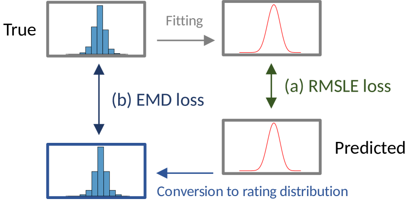
Figure 6: Two ways of measuring the loss of the predicted beta distribution (i.e., $L_{2}$). (a) As in Fig. 5, RMSLE is measured between the predicted shape parameters and the ground truth shape parameters (obtained by fitting to the ground truth rating distribution). (b) The predicted shape parameters are converted to a rating distribution, which is compared to the ground truth rating distribution in terms of EMD.

5.7.1 Impact of simultaneous learning.

In our simultaneous learning method, the neural network models predict both the rating distribution and the shape parameters of the beta distribution. In the conventional approach, only the rating distribution is predicted. We additionally test the case where the models predicts only the shape parameters of the beta distribution. The results are shown in Table III. Predicting only the beta distribution loses details of the original rating distribution, resulting in a lowered EMD in distribution prediction. However, the case of predicting the beta distribution outperforms the case of predicting the rating distribution in subjectivity regression, indicating the usefulness of our subjectivity modeling using beta distributions. Overall, the proposed simultaneous learning shows the best performance among the three cases.

5.7.2 Impact of fitting to beta distribution.

In our loss function, $L_{2}$ is measured between the beta distribution fitted to the ground truth rating distribution and the predicted beta distribution (using their shape parameters). Instead, it can be also measured without fitting, i.e., between the ground truth rating distribution and the rating distribution converted from the predicted beta distribution (Fig. 6). In this case, the weights ($w_{1}$, $w_{2}$, and $w_{3}$) are kept the same, but $w_{b}$ is set to 1 because any scale difference between the losses do not exist. The two cases are compared in Table IV. The performance of subjectivity regression is degraded significantly without fitting, while the performance of the other tasks remains almost the same.

5.8 Application to aesthetic image recommendation

Figure 7: Class boundaries of the ternary classification on the equilateral triangle of $b$, $d$, and $u$. The center point is set to the median value of each component for the training dataset, which is $(b,d,u)=(0.419,0.444,0.137)$.

Finally, we illustrate an application scenario where our subjectivity modeling can be applied.

Consider an image recommender application, where the image aesthetics of the recommended images is considered important. Even if an image is predicted to be aesthetically pleasing in terms of the mean rating, if a nonnegligible proportion of users would disagree on the prediction, then it would be better not to recommend the image to users in order to maximize the users’ satisfaction.

For this, the proposed framework can be used to filter out the images that are predicted to have high subjectivity levels. We perform ternary classification to classify an image as pleasing, unpleasing, or uncertain, based on the three probabilities obtained from our subjectivity modeling framework. The boundaries between the three classes are defined on the equilateral triangle of the three probabilities as shown in Fig. 7. The center point where the boundaries meet is set by the median values of $b$, $d$, and $u$ for the training dataset. Then, the recommendation rule is to recommend only the images classified to be pleasing. For comparison, we also consider the baseline rule to recommend an image if it is predicted to be aesthetically pleasing from binary classification.

We simulate the two rules on the test data of the AVA dataset using the trained ConvNeXT-T model. Their performance is measured by the satisfaction ratio, which is calculated as the average proportion of raters who voted scores higher than the threshold of binary classification over the recommended images. The obtained satisfaction ratios are 58.26% and 61.79% for the baseline rule and our rule, respectively. This improvement demonstrates the effectiveness of our framework in this application.

6 Conclusion

We proposed a unified probabilistic framework for modeling image aesthetics, particularly considering proper quantification of the subjectivity. The framework allowed us to model the rating distribution as a beta distribution and to obtain the probabilities of being definitely pleasing, being definitely unpleasing, and being uncertain simultaneously. The probability of being uncertain was used to define AesU, which is an intuitive subjectivity metric. We also proposed the simultaneous learning method to improve the performance of subjectivity prediction, which was confirmed by the experiments. Finally, we showed that our framework can be effective for aesthetics-based image recommendation.

References

- [1] Naila Murray, Luca Marchesotti and Florent Perronnin “AVA: A large-scale database for aesthetic visual analysis” In Proceedings of the IEEE Conference on Computer Vision and Pattern Recognition (CVPR), 2012, pp. 2408–2415 DOI: 10.1109/CVPR.2012.6247954
- [2] Chen Kang, Giuseppe Valenzise and Frédéric Dufaux “Predicting subjectivity in image aesthetics assessment” In Proceedings of the IEEE 21st International Workshop on Multimedia Signal Processing (MMSP), 2019, pp. 1–6
- [3] Audun Jøsang “Subjective Logic” Springer, 2016
- [4] Congcong Li and Tsuhan Chen “Aesthetic visual quality assessment of paintings” In IEEE Journal of Selected Topics in Signal Processing 3.2, 2009, pp. 236–252 DOI: 10.1109/JSTSP.2009.2015077
- [5] Eftichia Mavridaki and Vasileios Mezaris “A comprehensive aesthetic quality assessment method for natural images using basic rules of photography” In Proceedings of the IEEE International Conference on Image Processing (ICIP), 2015, pp. 887–891 DOI: 10.1109/ICIP.2015.7350927
- [6] Litian Sun, Toshihiko Yamasaki and Kiyoharu Aizawa “Photo aesthetic quality estimation using visual complexity features” In Multimedia Tools and Application 77.5, 2018, pp. 5189–5213
- [7] Xin Lu et al. “RAPID: Rating pictorial aesthetics using deep learning” In Proceedings of the ACM International Conference on Multimedia (MM), 2014, pp. 457–466
- [8] Long Mai, Hailin Jin and Feng Liu “Composition-preserving deep photo aesthetics assessment” In Proceedings of the IEEE Conference on Computer Vision and Pattern Recognition (CVPR), 2016
- [9] Dong Liu, Rohit Puri, Nagendra Kamath and Subhabrata Bhattacharya “Modeling image composition for visual aesthetic assessment” In Proceedings of the IEEE/CVF Conference on Computer Vision and Pattern Recognition (CVPR) Workshops, 2019
- [10] Kekai Sheng et al. “Revisiting image aesthetic assessment via self-supervised feature learning” In Proceedings of the AAAI Conference on Artificial Intelligence, 2020, pp. 5709–5716
- [11] Hui Zeng, Zisheng Cao, Lei Zhang and Alan C Bovik “A unified probabilistic formulation of image aesthetic assessment” In IEEE Transactions on Image Processing 29 IEEE, 2019, pp. 1548–1561
- [12] Jun-Tae Lee and Chang-Su Kim “Image aesthetic assessment based on pairwise comparison a unified approach to score regression, binary classification, and personalization” In Proceedings of the IEEE/CVF International Conference on Computer Vision (ICCV), 2019, pp. 1191–1200
- [13] Junjie Ke et al. “MUSIQ: Multi-scale image quality transformer” In Proceedings of the IEEE/CVF International Conference on Computer Vision (ICCV), 2021, pp. 5148–5157
- [14] Hossein Talebi and Peyman Milanfar “NIMA: Neural image assessment” In IEEE Transactions on Image Processing 27.8, 2018, pp. 3998–4011 DOI: 10.1109/TIP.2018.2831899
- [15] Qiuyu Chen et al. “Adaptive fractional dilated convolution network for image aesthetics assessment” In Proceedings of the IEEE/CVF Conference on Computer Vision and Pattern Recognition (CVPR), 2020
- [16] June Hao Ching, John See and Lai-Kuan Wong “Learning image aesthetics by learning inpainting” In Proceedings of the IEEE International Conference on Image Processing (ICIP), 2020, pp. 2246–2250
- [17] Dongyu She, Yu-Kun Lai, Gaoxiong Yi and Kun Xu “Hierarchical layout-aware graph convolutional network for unified aesthetics assessment” In Proceedings of the IEEE/CVF Conference on Computer Vision and Pattern Recognition (CVPR), 2021, pp. 8475–8484
- [18] Tae-Suh Park and Byoung-Tak Zhang “Consensus analysis and modeling of visual aesthetic perception” In IEEE Transactions on Affective Computing 6.3 IEEE, 2015, pp. 272–285
- [19] Won-Hee Kim, Jun-Ho Choi and Jong-Seok Lee “Objectivity and subjectivity in aesthetic quality assessment of digital photographs” In IEEE Transactions on Affective Computing 11.3 IEEE, 2020, pp. 493–506
- [20] Jian Ren et al. “Personalized image aesthetics” In Proceedings of the IEEE International Conference on Computer Vision (ICCV), 2017, pp. 638–647
- [21] Guolong Wang, Junchi Yan and Zheng Qin “Collaborative and attentive learning for personalized image aesthetic assessment” In Proceedings of the International Joint Conferences on Artificial Intelligence Organization (IJCAI), 2018, pp. 957–963
- [22] Leida Li et al. “Personality driven multi-task learning for image aesthetic assessment” In Proceedings of the IEEE International Conference on Multimedia and Expo (ICME), 2019, pp. 430–435 IEEE
- [23] Hancheng Zhu et al. “Personalized image aesthetics assessment via meta-learning with bilevel gradient optimization” In IEEE Transactions on Cybernetics IEEE, 2020
- [24] Pei Lv et al. “User-guided personalized image aesthetic assessment based on deep reinforcement learning” In IEEE Transactions on Multimedia IEEE, 2021
- [25] Yuzhe Yang et al. “Personalized image aesthetics assessment with rich attributes” In Proceedings of the IEEE/CVF Conference on Computer Vision and Pattern Recognition (CVPR), 2022, pp. 19861–19869
- [26] Hyeongnam Jang and Jong-Seok Lee “Analysis of deep features for image aesthetic assessment” In IEEE Access 9 IEEE, 2021, pp. 29850–29861
- [27] John A Hartigan and Pamela M Hartigan “The dip test of unimodality” In The annals of Statistics JSTOR, 1985, pp. 70–84
- [28] Karen Simonyan and Andrew Zisserman “Very deep convolutional networks for large-scale image recognition” In Proceedings of the International Conference on Learning Representations (ICLR), 2015
- [29] Kaiming He, Xiangyu Zhang, Shaoqing Ren and Jian Sun “Deep residual learning for image recognition” In Proceedings of the IEEE Conference on Computer Vision and Pattern Recognition (CVPR), 2016, pp. 770–778
- [30] Zhuang Liu et al. “A convnet for the 2020s” In Proceedings of the IEEE/CVF Conference on Computer Vision and Pattern Recognition (CVPR), 2022, pp. 11976–11986