Optimal Pre-Analysis Plans:
Statistical Decisions Subject to Implementability
(preliminary draft)

Abstract

What is the purpose of pre-analysis plans, and how should they be designed? We propose a principal–agent model where a decision-maker relies on selective but truthful reports by an analyst. The analyst has data access, and non-aligned objectives. In this model, the implementation of statistical decision rules (tests, estimators) requires an incentive-compatible mechanism. We first characterize which decision rules can be implemented. We then characterize optimal statistical decision rules subject to implementability. We show that implementation requires pre-analysis plans. Focussing specifically on hypothesis tests, we show that optimal rejection rules pre-register a valid test for the case when all data is reported, and make worst-case assumptions about unreported data. Optimal tests can be found as a solution to a linear-programming problem.

Keywords: Pre-analysis plans, Statistical decisions, Implementability
JEL codes: C18, D8, I23

1 Introduction

When writing up their studies, empirical researchers might cherry-pick the findings that they report. Cherry-picking distorts the inferences that we can draw from published findings, cf. Andrews and Kasy, (2019); Andrews et al., (2023). As a potential remedy, pre-analysis plans (PAPs) have become a precondition for the publication of experimental research in economics, for both field experiments and lab experiments. PAPs might enable valid inference by pre-specifying a mapping from the data to testing decisions or estimates, cf. Christensen and Miguel, (2018); Miguel, (2021). This might prevent the cherry-picking of results, and thus provide a remedy for the distortions introduced by unacknowledged multiple hypothesis testing. The widespread adoption of PAPs has not gone uncontested, however, and has been criticized for constraining our ability to learn from experiments.

In this article, we aim to clarify the benefits and optimal design of pre-analysis plans by modeling statistical inference as a mechanism-design problem (Myerson,, 1986; Kamenica,, 2019; Sinander,, 2023). To motivate this approach, note that, in single-agent statistical decision theory, rational decision-makers with preferences that are consistent over time have no need for the commitment device that is provided by a PAP. This holds in particular when a single decision-maker aims to construct tests that control size, or estimators that are unbiased; they have no reason to “cheat themselves.” The situation is different, however, when there are multiple agents with conflicting interests, or when preferences are not consistent over time.

In this article, we provide detailed guidance for practitioners, including both decision-makers (e.g., readers, editors) and data analysts (e.g., study authors). From the decision-makers’ perspective, we describe how tests, estimators, or other decision rules can be implemented by requiring pre-analysis plans. We then focus on hypothesis tests in particular, and show, from the analysts’ perspective, how to derive optimal pre-analysis plans, which maximize power while controlling size and maintaining implementability. We also provide software (an interactive web app) to facilitate the design of optimal pre-analysis plans.

Examples

In our model, we consider the interaction between a decision-maker and an analyst with private information and conflicting interests. One example of such a conflict of interest is between a researcher (analyst) who wants to reject a hypothesis, and a reader of their research (decision-maker) who wants a valid statistical test of that same hypothesis; the relevant decision here is whether to reject the null hypothesis. Another example is the conflict of interest between a researcher (analyst) who wants to get published, and a journal editor (decision-maker) who only wants to publish studies on effects that are large enough to be interesting; the relevant decision here is whether to publish a study. A third example is the conflict of interest between a pharmaceutical company (analyst) who wants to sell drugs, and a medical regulatory agency (decision-maker) who wants to protect patient health; the relevant decision here is whether to approve a drug.

Model and timeline

The mechanism-design approach that we propose takes the perspective of a decision-maker who wants to implement a statistical decision rule. Not all rules are implementable, however, when the analyst has divergent interests and private information. This mechanism-design perspective allows us to stay close to standard statistical theory, while taking into account the constraints that are a consequence of the social nature of research.

The timeline of our model is as follows. Before observing the data, the analyst might send a pre-analysis message $M$ to the decision-maker. This message might be in the form of a pre-analysis plan. The full data which are potentially observed by the analyst are given by a vector $X=(X_{1},\ldots,X_{k})$, and are distributed according to some true, unknown state $\theta$. The components of $X$ might, for instance, correspond to the outcomes of different hypothesis tests, or to estimates for different model specifications. Not all of these components are actually available to the analyst, however. Instead, the analyst only observes $X_{i}$ for $i\in J$, where the set of available components $J\subseteq\{1,\ldots,k\}$ is private information of the analyst. The analyst gets to choose a subset $I\subseteq J$ of observations, and then reports $(X_{I},I)$ to the decision-maker, who takes a decision $A\in\mathcal{A}\subseteq\mathbb{R}$. The analyst always prefers a higher value for $A$. We consider different objectives for the decision-maker, including, in particular, statistical testing subject to size control, in which case $A$ is the probability of rejecting the null hypothesis.

In this model, the analyst might hide information from the decision-maker, but they may not lie about the components they report. Put differently, our model is one of partial verifiability. The potential value of a pre-analysis message in this setting comes from the fact that it allows the analyst to share private information (i.e., expertise) with the decision-maker, in a way that would not be incentive compatible if a message could only be sent after seeing the data. The analyst might have private information regarding the availability of components $J$, and regarding the state of the world $\theta$. Availability of components $X_{i}$ might be restricted for various reasons: Not every estimate or test that is a priori conceivable is actually at the analyst’s disposition. Prior uncertainty about component availability allows for plausible deniability by the analyst. Experiments might not have been run, or data might not have been collected.

Implementable decision rules

We first characterize the set of implementable statistical decision rules, which is independent of decision-maker preferences. We show that implementable decision rules are required to be monotonic in the reported set of components $I$, in terms of set inclusion, given the pre-analysis message, and given $X$. Put differently, reporting more results can never make the analyst worse off. Implementable decision rules furthermore need to be compatible with truthful revelation of analyst private information prior to observing any data (Myerson,, 1986). This condition is equivalent to the conditions satisfied by proper scoring rules (Savage,, 1971; Gneiting and Raftery,, 2007).

Implementable rules can be implemented using different mechanisms. One possible implementation allows the analyst to choose from a restricted set of decision rules, where each of these rules needs to be monotonic in $I$, before seeing the data. This corresponds to the actual practice of pre-analysis plans, where the analyst chooses a decision rule before the data becomes available.

The set of implementable rules can be characterized as a convex polytope. If the decision-maker objective is convex, and in particular if it is linear, then the optimal implementable rule is necessarily an extremal point of this polytope (Vanderbei et al.,, 2020). Pre-analysis messages allow the decision-maker to implement a larger set of decision rules than would be available without such messages.

Optimal implementable hypothesis tests

We next turn to the specific problem of finding optimal implementable hypothesis tests. Such tests are required to satisfy size control conditional on both the state of the world and on analyst private information that is available before observing the data. We show that the optimal implementable test, for the decision-maker, can be implemented by (i) requiring the analyst to choose an arbitrary full-data test, which is a function of all components $X$, where this test controls size, and then (ii) implementing this test, making worst-case assumptions about any unreported components $X_{i}$. The analyst’s problem of finding a full-data test that maximizes expected power for this mechanism can again be cast as a linear programming problem. We provide an interactive app that allows the analyst to solve this problem, based on their prior for both data availability $J$ and for the state of the world $\theta$. The output of this app can then serve as a basis for their pre-analysis plan.

Roadmap

The rest of this article is structured as follows. We conclude this introduction with a review of some related literature. In Section 2, we present a motivating example concerning statistical testing and p-hacking. In Section 3, we introduce the general model. In Section 4, we characterize implementable decision rules. In Section 5, we characterize optimal implementable hypothesis tests. Appendix A contains all proofs. Appendix B discusses some numerical examples of optimal hypothesis tests subject to the constraint of implementability.

1.1 Related literature

Our article speaks, first, to the current debates around pre-registration – and other possible reforms – in empirical economics and other social- and life-sciences; cf. Christensen and Miguel, (2018); Miguel, (2021). In doing so, our article applies some of the insights from mechanism design and information design (Myerson,, 1986; Kamenica,, 2019; Sinander,, 2023) to the settings of statistical decision theory and statistical testing, (Wald,, 1950; Savage,, 1951; Lehmann and Romano,, 2006). More broadly, our article contributes to a literature that spans statistics, econometrics and economic theory, and which models statistical inference in multi-agent settings. We differ from other contributions to this literature, in that we focus on the role of implementability as a constraint on statistical decision rules, which rationalizes pre-analysis plans, and on the derivation of optimal decision rules subject to the constraint of implementability.

Drawing on classic references (Tullock,, 1959; Sterling,, 1959; Leamer,, 1974), Glaeser, (2006) considers the role of incentives in empirical research. A number of recent contributions model estimation and testing within multiple-agent settings, including Glazer and Rubinstein, (2004); Mathis, (2008); Chassang et al., (2012); Tetenov, (2016); Di Tillio et al., (2021, 2017); Spiess, (2018); Henry and Ottaviani, (2019); McCloskey and Michaillat, (2020); Libgober, (2020); Yoder, (2020); Williams, (2021); Abrams et al., (2021); Viviano et al., (2021). In this literature, Banerjee et al., (2020); Frankel and Kasy, (2022); Andrews and Shapiro, (2021); Gao, (2022) consider the communication of scientific results to an audience with priors, information, or objectives that might differ from the sender’s.

The literature on Bayesian persuasion (Kamenica and Gentzkow,, 2011; Kamenica,, 2019; Curello and Sinander,, 2022), like the present article, considers a sender with information unavailable to a receiver, where sender and receiver have divergent objectives. One important way in which our model differs from that of Bayesian persuasion is that in our model the signal space of the analyst is restricted to the truthful but selective reporting of data. This restriction implies that the concavification argument central to Bayesian persuasion does not apply.

2 A motivating example

Before we introduce our general model, consider the following hypothesis-testing problem, where there is a decision-maker and an analyst: The full data consists of two normally distributed components, $X=(X_{1},X_{2})$, with $X_{i}\sim\mathcal{N}(\theta,1)$, independently across components. The $X_{i}$ might for instance correspond to experimental estimates of an average treatment effect, for two different experimental sites. The analyst observes the subvector $X_{J}$. The component $i\in\{1,2\}$ is observed (i.e., $i\in J$) with probability $\eta_{i}$, again independently across components. Put differently, $\eta_{i}$ is the decision-maker’s a-priori probability that the analyst successfully implemented an experiment at site $i$.

The decision-maker is interested in testing the null hypothesis $H_{0}:\theta\leq 0$. The analyst, on the other hand, aims to maximize the probability of rejection. The decision-maker does not know which components are actually available, that is, they do not know $J$. The analyst knows which components are available. Upon learning the data $X_{J}$, the analyst chooses the subset $I\subseteq J$, and reports $(X_{I},I)$ to the decision-maker, who then rejects the null with probability $A=\mathbf{a}(X_{I},I)\in[0,1]$. How should the decision-maker choose the testing rule $\mathbf{a}$ that maps the reported data to a rejection probability?

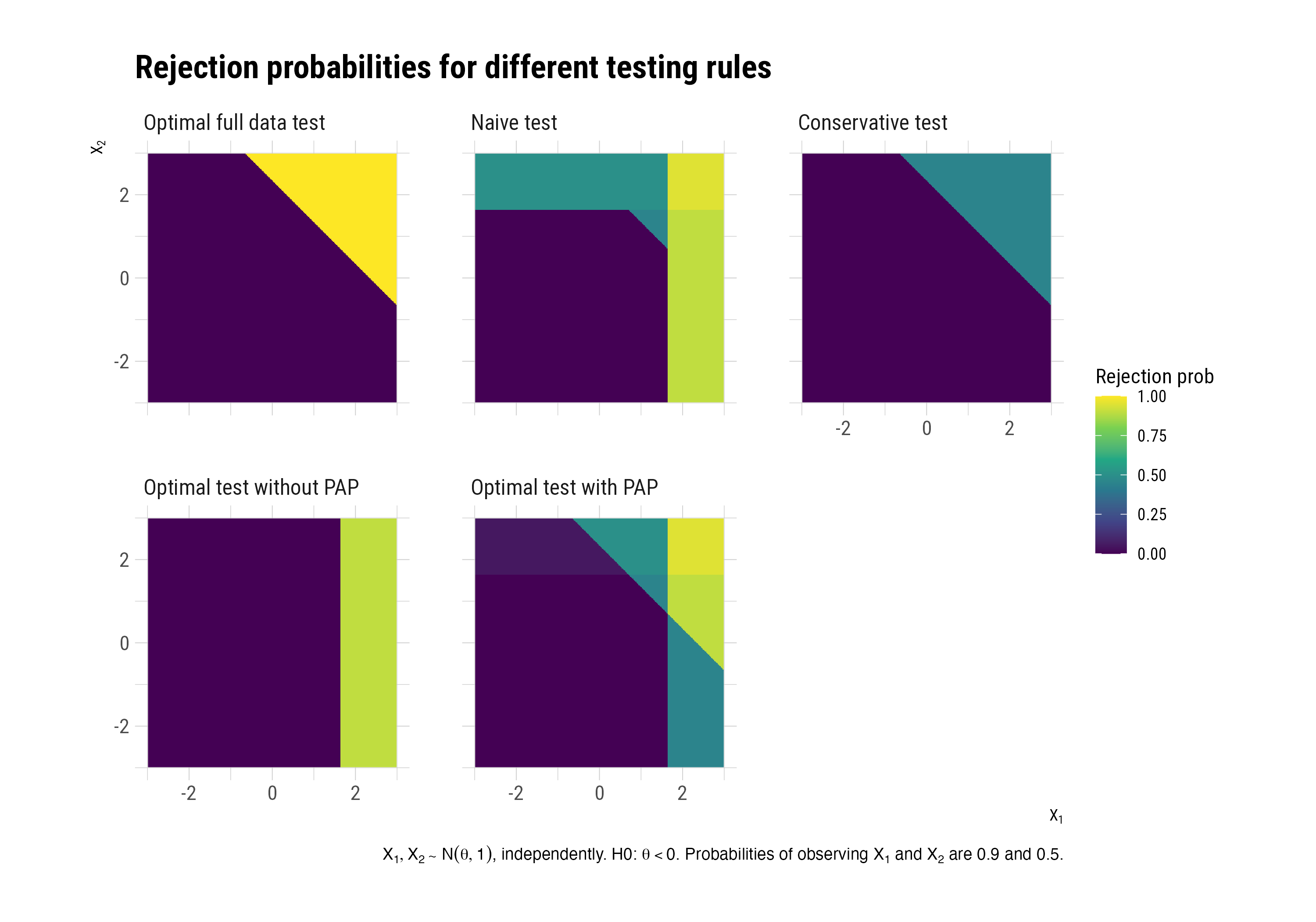
Figure 1: Comparison of testing rules

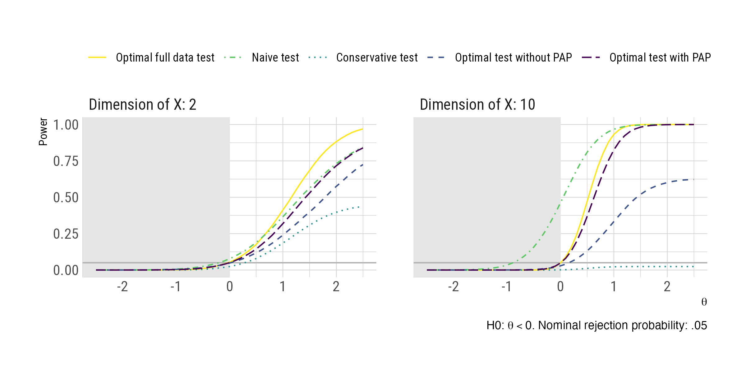
Figure 2: Power curves

Five testing rules

We compare five different testing rules, $\mathbf{a}_{0}$ through $\mathbf{a}_{4}$. For each of these testing rules, Figure 2 shows the rejection probability as a function of $(X_{1},X_{2})$, assuming that $\eta=(0.9,0.5)$. This conditional rejection probability given $X$ averages over the availability of components, $J$. The left panel of Figure 2 shows the corresponding power curves, i.e., the rejection probability as a function of $\theta$, averaging over the distribution of both $X$ and $J$.

Our benchmark is the optimal test using all the data. This test is not, in general, feasible, since not all components are always available. We have that $Z=\tfrac{1}{\sqrt{2}}(X_{1}+X_{2})\sim\mathcal{N}({\sqrt{2}}\cdot\theta,1)$ is a sufficient statistic for $\theta$. Since this statistic satisfies the monotone likelihood ratio property, the Neyman–Pearson Lemma implies that the uniformly most powerful test of level $\alpha$ is given by $\mathbf{a}_{0}(X)=\boldsymbol{1}(Z>z),$ where $z=\Phi^{-1}(1-\alpha)$; cf. Theorem 3.4.1 in Lehmann and Romano, (2006).

Consider next the naive test which ignores potentially selective reporting by the analyst. This test acts as if the reported components $I$ are the full data available to the analyst, and implements the corresponding uniformly most powerful test,

$$\mathbf{a}_{1}(X_{I},I)=\boldsymbol{1}\left(\frac{1}{\sqrt{|I|}}\sum_{i\in I}X_{i}>z\right).$$

The best response of the analyst to this naive testing rule involves selective reporting (“p-hacking”), where $I^{*}\in\operatorname*{argmax\;}_{I\subseteq J}\mathbf{a}(X_{I},I)$. The problem with this naive test is that it does not control size. Selective reporting by the analyst implies that the probability of rejection under the null is not bounded by $\alpha$.

We might correct for such selective reporting by making worst-case assumptions about all unreported components. This results in the conservative test,

$$\mathbf{a}_{2}(X_{I},I)=\boldsymbol{1}\left(\frac{1}{\sqrt{2}}(X_{1}+X_{2})>z\text{ and }I=\{1,2\}\right).$$

If there are components which are not reported, then the null is not rejected. This conservative test implies a probability of rejection given $X$ of $\eta_{1}\cdot\eta_{2}\cdot\boldsymbol{1}\left(\frac{1}{\sqrt{2}}(X_{1}+X_{2})>z\right).$ The conservative test controls size, but does not have good power properties.

As we show more generally in Section 4 and Section 5 below, the optimal test without a pre-analysis plan can be implemented by selecting a full-data test of level $\alpha$. When not all data are reported, the decision-maker needs to assume the worst about the unreported components, and then implements the corresponding full-data test. The decision-maker can choose the full-data test to maximize (ex-ante) expected power, averaging over their prior for $\theta$.

One possible full-data test ignores $X_{2}$, which is less likely to be observed in our numerical example, and rejects based on $X_{1}$ alone. This results in the test

$$\mathbf{a}_{3}(X_{I},I)=\boldsymbol{1}\left(X_{1}>z\text{ and }1\in I\right).$$

This test implies a probability of rejection given $X$ of $\eta_{1}\cdot\boldsymbol{1}\left(X_{1}>z\right).$ This test is optimal for some parameter values, while in general the optimal test depends on the prior over $\theta$.

We lastly get to the optimal test with a PAP. The optimal test with a PAP is of the same form as the optimal test without a PAP, except that the analyst gets to choose the full data test, prior to seeing any data. Recall that in our example the analyst knows the components $J$ that are available before possibly reporting a PAP, but we assume that they have no private information regarding $\theta$. (We relax this assumption in our general setup below.) The optimal implementable solution is of the following form. The analyst communicates which components are available as pre-analysis message $M=J$, and the test is given by

$$\mathbf{a}_{4}(M,X_{I},I)=\boldsymbol{1}\left(\frac{1}{\sqrt{|M|}}\cdot\sum_{i\in M}X_{i}>z\text{ and }M\subseteq I\right).$$

That is, the analyst commits to reporting all components in $J$, and for that set of components, the most powerful test is implemented.

Comparing size and power

The left panel of Figure 2 plots the power curves for the five testing rules, for $n=\dim(X)=2$, which is the case that we have considered thus far. The right panel shows analogous plots for $n=10$, with the components of $\eta$ evenly distributed over a grid from $.5$ to $.9$. The latter case illustrates the contrasts between testing rules more starkly.

A number of observations are worth emphasizing here. First, the naive test does not control size. For $n=10$, the probability of rejection for $\theta=0$ is close to $.5$, instead of the nominal size of $.05$. This is due to selective reporting (“p-hacking”). Second, the conservative test can be very conservative. Since it only rejects when all components of $X$ are reported, the probability of rejection under the alternative can be arbitrarily small, and remains below the nominal size of $.05$ for our example with $n=10$. Third, the optimal test without a PAP does considerably better. It controls size, and is actually strictly conservative under the null. At the same time, it has non-trivial power, which greatly exceeds that of the conservative test. It remains far from optimal, however. The optimal test with a PAP, lastly, controls size exactly under the null. Furthermore, its power under the alternative considerably exceeds that of the optimal test without a PAP.

From our example to the general model

Our motivating example is a special case of the general model that we lay out in Section 3. The general model allows for cases where the researcher also has private information about $\theta$, and where the researcher only has partial information about availability $J$ of the data. The general model also covers decision problems other than testing, including estimation and treatment choice.

3 Setup

We next describe our general setup, which will be discussed for the rest of this paper. This setup consists of a game between a decision-maker and an analyst. This game is summarized in Assumption 1. The corresponding timeline is shown in Figure 3.

Assumption 1 (Setup).

The game between decision-maker and analyst unfolds as follows:

1. The decision-maker selects a message space $\mathcal{M}$ and commits to a decision function $\mathbf{a}:(M,X_{I},I)\mapsto A\in\mathcal{A}$.

2. The analyst observes the private signal $\pi$ and sends a message $M\in\mathcal{M}$ to the decision-maker.

3. The analyst observes the realization $(X_{J},J)$ of available data and selects a subset $I\subseteq J$.

4. The decision-maker observes the message $M$, the subset $I$, and the data $X_{I}$, and implements the decision $A=\mathbf{a}(M,X_{I},I)$.

The analyst and the decision-maker share a common prior $\operatorname{P}$ over the signal $\pi$, the parameter $\theta$, the availability $J$, and the data $X$. This prior satisfies that the conditional distribution of $X$ only depends on $\theta$, i.e., $X|\theta,J,\pi\stackrel{{\scriptstyle d}}{{=}}X|\theta$.

Figure 3: Timeline

Discussion

This is a game of partial verifiability. The report $X_{I}$ is always truthful given $I$, but the non-availability of the components of $\{1,\ldots,k\}\setminus J$ cannot be verified by the decision-maker. Selective reporting, where not all available components are reported ($I\varsubsetneq J$), corresponds to p-hacking, or specification searching. Mis-reporting of $X_{I}$, which corresponds to scientific fraud, is not allowed in our setting.

The private signal $\pi$ corresponds to analyst expertise. The signal $\pi$ might be informative about $\theta$, corresponding to knowledge about which hypotheses are likely to be correct, about the likely magnitude of effect sizes, etc. The signal $\pi$ might also be informative about $J$, corresponding to knowledge about the viability of different identification approaches, the availability of experimental sites, etc.

There is prior uncertainty of the decision-maker regarding the availability of components $J$. Without such uncertainty, the mechanism design problem would be trivial, and the decision-maker would simply require the analyst to report everything. Prior uncertainty allows for “plausible deniability,” because the decision-maker maker does not know the full set of results from which the reported results were selected.

In Assumption 1, we have left the message space $\mathcal{M}$ for the pre-analysis message $M$ unrestricted. We will later encounter different, equivalent choices for $\mathcal{M}$: The message $M$ might directly communicate the analyst signal $\pi$, or their corresponding posterior, in the spirit of the revelation principle in mechanism design. Alternatively, the message $M$ might choose a decision function $\mathbf{a}$ from a restricted set, in the spirit of “aligned delegation” (Frankel,, 2014). This latter formulation corresponds more directly to the practice of pre-analysis plans.

Objectives

We have not yet described the objectives of either the decision-maker or the analyst. We allow for conflicting objectives, which render the mechanism-design problem non-trivial. By contrast, we have imposed common priors, so that there are no agency issues driven by divergent beliefs.

We leave the decision-maker’s objective unspecified at this point. This allows us to first study implementability as a general constraint on the set of decision-functions available to the decision-maker. This constraint does not depend on the decision-maker objective. We also do not impose that the decision-maker is an expected utility maximizer. This allows us to also study frequentist statistical decision-problems subject to the constraint of implementability, including hypothesis testing subject to size control, and unbiased estimation, in addition to Bayesian decision problems.

By contrast, we do assume that the analyst is an expected utility maximizer. We furthermore impose the following restriction on their utility function for most of our discussion.

Assumption 2 (Monotonic analyst utility).

The analyst is an expected utility maximizer with utility $v(A)$, for a strictly monotonically increasing function $v$.

The analyst always prefers a higher outcome $A\in\mathcal{A}$. In the context of testing, the analyst always prefers to reject the null hypothesis. In the context of publication decisions, the analyst always would like their paper to be published. In the context of drug approval, the pharmaceutical company always would like their drug to be approved.

4 Implementability

Conventional statistical decision theory considers decision functions that map the available information into statistical decisions (Wald,, 1950; Savage,, 1951). In our context, such decision functions $\bar{\mathbf{a}}(\pi,X_{J},J)$ map the signal $\pi$, the available data $X_{J}$, and the component set $J$ into decisions $A$. We will call such functions $\bar{\mathbf{a}}$ reduced-form decision functions.

In our setting, not all such decision functions are available to the decision-maker, because of analyst private information and conflicting objectives. In this section, we will characterize the set of implementable reduced form decision functions $\bar{\mathbf{a}}$ which are consistent with analyst utility maximization. This leads to constrained versions of conventional statistical decision problems, including hypothesis testing and point estimation. We will show that implementation, in general, requires the use of pre-analysis messages.

4.1 Which decision functions can be implemented?

The analyst’s optimal message $M^{*}$ and reported set $I^{*}$ maximize analyst expected utility $\operatorname{E}[v(\mathbf{a}(M,X_{I},I))]$, given the decision rule $\mathbf{a}$. Here $M^{*}$ and $I^{*}$ are random elements, where $M^{*}$ is measurable with respect to $\pi$, and $I^{*}$ is measurable with respect to $\pi,X_{J},J$. Analyst expected utility maximization and strict monotonicity of $v$ imply

$$I^{*} \in\operatorname*{argmax\;}_{I\subseteq J}\mathbf{a}(M^{*},X_{I},I),\text{ and}$$

$$M^{*} \in\operatorname*{argmax\;}_{M\in\mathcal{M}}\operatorname{E}[v(\mathbf{a}(M,X_{I^{*}},I^{*}))|\pi].$$ (1)

Consider now reduced-form decision functions $\bar{\mathbf{a}}(\pi,X_{J},J)$ that map the information available to the analyst to a decision-maker action. We say that a function $\bar{\mathbf{a}}$ is implementable if it is consistent with analyst utility maximization.

Definition 1 (Implementable reduced-form decision rules).

A reduced form decision function $\bar{\mathbf{a}}(\pi,X_{J},J)$ is implementable if there exists a decision function $\mathbf{a}$ with best responses $M^{*},I^{*}$ such that

$$\bar{\mathbf{a}}(\pi,X_{J},J)=\mathbf{a}(M^{*},X_{I^{*}},I^{*})$$

almost surely.

The following theorem provides a complete characterization of implementable reduced-form decision rules in our setting. The proof of this theorem, and all subsequent proofs, can be found in Appendix A.

Theorem 1 (Implementability).

Under Assumptions 1 and 2, a reduced-form decision function $\bar{\mathbf{a}}(\pi,X_{J},J)$ is implementable if and only if there is some $\tilde{\mathbf{a}}$ such that $\bar{\mathbf{a}}(\pi,X_{J},J)=\tilde{\mathbf{a}}(\pi,X_{J},J)$ almost surely, and both of the following two conditions hold:

1. Truthful message: For all $\pi,\pi^{\prime}$,

   $$\operatorname{E}[v(\tilde{\mathbf{a}}(\pi^{\prime},X_{J},J))|\pi]\leq\operatorname{E}[v(\tilde{\mathbf{a}}(\pi,X_{J},J))|\pi].$$ (2)

2. Monotonicity: For all $\pi,X,J$ and $I\subseteq J$,

   $$\tilde{\mathbf{a}}(\pi,X_{I},I)\leq\tilde{\mathbf{a}}(\pi,X_{J},J).$$ (3)

Theorem 1 characterizes which reduced-form decision functions $\bar{\mathbf{a}}(\pi,X_{J},J)$ can be implemented, but it does not tell us how to implement them. The following Proposition 1 shows two different, canonical ways of implementing any such function. The first implementation uses truthful revelation of analyst signals. The second implementation uses delegation, where the analyst is effectively allowed to choose the decision function from a pre-specified, restricted set $\mathcal{B}$. This second implementation corresponds closely to the actual practice of pre-analysis plans. Here, the analyst pre-specifies a mapping $b$ from the reported data $(X_{J},J)$ to the decision $A=b(X_{J},J)$. Proposition 1 shows that restricting attention to implementation by such pre-analysis plans is without loss of generality.

Proposition 1 (Implementation).

Under Assumptions 1 and 2, a reduced-form decision rule $\bar{\mathbf{a}}$ can be implemented if and only if either of the following two conditions holds:

1. Implementation by truthful revelation: $\bar{\mathbf{a}}$ can be implemented with a decision rule $\mathbf{a}$ for which

   $$\mathbf{a}(\pi,X_{J},J)=\bar{\mathbf{a}}(\pi,X_{J},J),$$

   where the message space is the set of all possible signals $\pi$.

2. Implementation by delegation (pre-analysis plan): $\bar{\mathbf{a}}$ can be implemented with a decision rule $\mathbf{a}$ for which

   $$\mathbf{a}(b,X_{J},J)=b(X_{J},J),$$

   where $b$ is restricted to lie in some set $\mathcal{B}$ that acts as the message space.

4.2 Alternative characterizations of implementability

Having characterized implementable decision functions in general, we next discuss implementability for the special case of linear analyst utility $v$ and convex action space $\mathcal{A}$. We also discuss the connection of truthful revelation to proper scoring, as well as possible simplicity restrictions on pre-analysis plans.

The set of implementable rules as a convex polytope

In addition to Assumptions 1 and 2, assume for a moment that the action space $\mathcal{A}\subseteq\mathbb{R}$ is convex, and that analyst utility is linear – without additional loss of generality, $v(A)=A$. The leading examples involve binary decisions, where we interpret $A$ as the probability of a positive decision. Binary decisions occur for statistical testing, as discussed in Section 5 below, as well as for publication decisions, drug approval, etc. Linearity is without loss of generality for the case of binary decisions; in this case, it follows from expected utility maximization. Suppose finally that $\pi$ has finite support.

Under these additional assumptions, we get that the set of implementable reduced form decision functions $\bar{\mathbf{a}}$ is given by a convex polytope, characterized by the following constraints.

$$\bar{\mathbf{a}}(\pi,X_{J},J) \in\mathcal{A},$$ (Support)

$$\bar{\mathbf{a}}(\pi,X_{I},{I})-\bar{\mathbf{a}}(\pi,X_{J},{J}) \leq 0 \forall\;\pi,X_{J},J,I\subseteq J,$$ (Monotonicity)

$$\sum_{X_{J},J}\left(\bar{\mathbf{a}}({\pi^{\prime}},X_{J},J){-}\bar{\mathbf{a}}({\pi},X_{J},J)\right)\>\operatorname{P}_{\pi}(X_{J},J) \leq 0 \forall\;\pi^{\prime},\pi.$$ (Truthful message)

In the last inequality, $\operatorname{P}_{\pi}$ is a shorthand for the analyst’s posterior distribution conditional on $\pi$.

If, furthermore, the decision-maker objective is linear in $\bar{\mathbf{a}}$, as is the case for a Bayesian decision-maker and binary actions, or if it is linear with an additional linear constraint, as is the case for expected power maximization subject to size control, then the problem of finding the optimal implementable reduced form decision function becomes a linear programming problem. Efficient algorithms exist for numerically solving such problems, cf. Vanderbei et al., (2020). We will return to this point in Section 5 below. We leverage such linear programming algorithms in our interactive app for finding optimal PAPs.

Truthful revelation of beliefs and proper scoring

Condition (2) in Theorem 1 ensures that the analyst reveals their relevant prior information truthfully. Condition (2) is equivalent to the definition of a proper scoring rule, as introduced by Savage, (1971). The theory of proper scoring rules has regained importance in the more recent statistics and machine learning literature, cf. Gneiting and Raftery, (2007).

Given a reduced form decision rule $\bar{\mathbf{a}}$, define

$$S(\pi^{\prime},\pi)=\operatorname{E}_{\pi}[v(\bar{\mathbf{a}}(\pi^{\prime},X_{J},J))].$$ (4)

The expectation $\operatorname{E}_{\pi}$ is taken over the conditional prior distribution $\operatorname{P}_{\pi}$ of $X_{J},J$ given $\pi$. Denote the Euclidean inner product for functions of $X_{J},J$ (understood here as values, rather than as random variables) by $\langle f(\cdot),g(\cdot)\rangle=\sum_{X_{J},J}f(X_{J},J)\cdot g(X_{J},J)$. Here we assume for simplicity that $X$ has finite support, though the argument generalizes. We obtain the following characterization, which was first stated by Savage, (1971) and is restated as Theorem 2 in Gneiting and Raftery, (2007).

Proposition 2 (Proper scoring rule).

Condition (2), the truthful message condition, holds for all $\pi,\pi^{\prime}$ if and only if there exists a convex function $G$ with sub-gradient $G^{\prime}$, where $G(\operatorname{P}_{\pi})=S(\pi,\pi)$ on the support of $\pi$, such that $S(\pi^{\prime},\pi)=G(\operatorname{P}_{\pi^{\prime}})+\langle G^{\prime}(\operatorname{P}_{\pi^{\prime}},\cdot),\operatorname{P}_{\pi}-\operatorname{P}_{\pi^{\prime}}\rangle.$

Simple pre-analysis plans

Item 2 of Proposition 1 shows that reduced form decision rules can be implemented by delegation: The decision-maker offers a set $\mathcal{B}=\{b:\;(X_{I},I)\mapsto\mathcal{A}\}$ of permissible pre-analysis plans (decision functions). The analyst then commits to one of the decision functions $b\in\mathcal{B}$ before access to the data.

In practice, some pre-analysis plans may be unrealistically complicated, and we may wish to restrict attention to a smaller set $\mathcal{B}_{0}$ of simpler mappings. The decision-maker’s choice would then be restricted to $\mathcal{B}\subseteq\mathcal{B}_{0}$ as a subset of feasible mappings.

4.3 Are pre-analysis messages needed?

Aligned objectives

Why does implementability in our setting appear to require a pre-analysis message, if that is not the case in conventional statistical decision theory? Assume for a moment that analyst and decision-maker share the same objective function. In this case, is there any need for a pre-analysis message? The answer is no.

To see this, consider the following variant of our setup. Suppose everything is as in Assumption 1 (Figure 3), except that the analyst gets to choose the message $M$ after they observe the data $X_{J},J$. Put differently, the analyst cannot provide a verifiable time-stamp for their message $M$ to the decision-maker. The following observation states that in this modified setting, where there is no pre-analysis message, the decision-maker can still implement the first-best reduced-form decision rule, provided that preferences are aligned.

Proposition 3 (First-best decisions for aligned preferences).

Under the modified Assumption 1 where the message $M$ can depend on the realization $(X_{J},J)$, assume that analyst and decision-maker are expected utility maximizers who share the same utility function $u(A,\theta)$. Then the decision-maker’s first-best reduced-form decision rule $\bar{\mathbf{a}}(\pi,X_{J},J)$ is implementable.

As Proposition 3 shows, pre-analysis messages only become potentially useful in the presence of both private information and misaligned preferences.

Implementability without pre-analysis message

We next characterize the set of decision functions $\bar{\mathbf{a}}$ that are implementable without a pre-analysis message, when objectives can be misaligned. In this case, the implementable functions are exactly the functions $\bar{\mathbf{a}}(\pi,X_{J},J)$ that satisfy monotonicity with respect to set inclusion for the index set $J$ given $X$, and that do not depend on $\pi$. Analyst expertise can thus not be used to improve decisions at all, in the absence of a pre-analysis message. The proof of the following proposition parallels the proof of Theorem 1.

Proposition 4 (Implementability without pre-analysis message).

Under Assumptions 1 and 2, with the additional constraint that there is no pre-analysis message, a reduced-form decision function $\bar{\mathbf{a}}$ is implementable if and only if there is a function $\tilde{\mathbf{a}}$ with almost surely $\bar{\mathbf{a}}(\pi,X_{J},J)=\tilde{\mathbf{a}}(X_{J},J)$ and

$$\tilde{\mathbf{a}}(X_{I},I)\leq\tilde{\mathbf{a}}(X_{J},J)$$ (5)

for almost all $X,J$ and all $I\subseteq J$.

5 Frequentist hypothesis testing

We next specialize our general framework to the setting of frequentist hypothesis testing. In this setting, the decision-maker decides whether to reject a null hypothesis. We assume that the decision-maker wants to maximize expected power subject to size control. The analyst, however, always prefers a rejection of the null hypothesis.

Building on our previous results, we characterize the set of implementable testing rules that satisfy size control, in Section 5.2. We provide a simple mechanism that allows the decision-maker to implement the optimal testing rule. This mechanism requires a pre-analysis plan, where the analyst may choose any full-data test that satisfies size control, and the decision-maker then makes worst-case assumptions about any unreported data. This mechanism solves the decision-maker’s problem.

In Section 5.3 we then consider the analyst’s problem of finding an optimal response to this mechanism, and show that they have to solve a linear programming problem to find the optimal pre-analysis plan. We provide software to solve this problem of the analyst. We also characterize the set of possible solutions to the analyst’s problem, by describing the set of extremal points of their feasible set.

Throughout, we focus on the problem of testing a single (joint) hypothesis, and leave an extension to deciding which of multiple hypotheses to reject for future work.

5.1 Decision-maker and analyst objectives

Assume that the decision $A\in[0,1]$ represents the probability, given $(M,X_{J},J)$, of rejecting the null hypothesis $\theta\in\Theta_{0}$. Suppose that the analyst is an expected utility maximizer, who ex-post only cares about the binary testing decision. Ex-ante, the analyst thus wants to maximize expected power. It follows that their utility is linear in $A$. We can then make the following normalizing assumption, without loss of generality.

Assumption 2’ (Power analyst utility).

Analyst utility is

$$v(A)=A.$$

The decision-maker also wants to maximize expected power, but subject to the constraint of size control under the null hypothesis.

Definition 2 (Size control).

We say that a reduced-form decision rule $\bar{\mathbf{a}}$ controls size at level $\alpha\in(0,1)$ if

$$\sup_{\mathclap{\pi,\theta\in\Theta_{0},J\subseteq\{1,\ldots,n\}}}\operatorname{E}[\bar{\mathbf{a}}(\pi,X_{J},J)|\theta,\pi,J] \leq\alpha.$$ (6)

Recall that we imposed, in Assumption 1, that the conditional distribution of $X$ only depends on $\theta$, that is, $X|\theta,J,\pi\stackrel{{\scriptstyle d}}{{=}}X|\theta.$ Under this assumption, the conditional expectation $\operatorname{E}[\bar{\mathbf{a}}(\pi,X_{J},J)|\theta,\pi,J]$ is well-defined even outside the joint support of $\pi,\theta,J$, as long as $\theta$ is within its marginal support.

5.2 Decision-maker solution: Pre-specified full-data tests

The implementability results of Section 4 allow us to characterize optimal pre-analysis plans for hypothesis testing as follows.

Theorem 2 (Optimal pre-analysis plans with size control).

Define $\mathcal{T}$ to be the class of measurable full-data tests $t:\mathcal{X}\rightarrow[0,1]$ satisfying size control, $\sup_{\theta\in\Theta_{0}}\operatorname{E}[t(X)|\theta]\leq\alpha$. Under Assumption 1 and Assumption 2’, the power-maximizing decision rule subject to the constraints of implementability (Definition 1) and size control (Definition 2) can be implemented by requiring the analyst to communicate, as a pre-analysis message, a full-data test $t\in\mathcal{T}$, and then rejecting the null with conditional probability

$$b(X_{I},I)=\inf_{X^{\prime};\;X^{\prime}_{I}=X_{I}}t(X^{\prime}).$$

This result builds on the general characterizations of Theorem 1 and Proposition 1. To get further intuition for Theorem 2 note, first, that it is sufficient to verify size control for the full-data test $t$. The reason is that implementable reduced-form decision rules must fulfill the monotonicity constraint (3). Subject to monotonicity in $I$, size control of $\bar{\mathbf{a}}$ in the sense of Definition 2 is equivalent to size control for the full-data test $\bar{\mathbf{a}}(\pi,X,\{1,\ldots,k\})$.

Note, second, that for optimal reduced-form testing rules the monotonicity constraint is in general binding, since both decision-maker and analyst aim to maximize expected power, subject to the constraints. For optimal rules it is therefore without loss of generality to assume $\bar{\mathbf{a}}(\pi,X_{J},J)=\inf_{X^{\prime};\;X^{\prime}_{J}=X_{J}}t(X^{\prime})$, which can be implemented by $b$ as in the statement of the theorem.

5.3 Analyst solution: Linear programming

Theorem 2 solves the optimal testing problem from the decision-maker’s perspective: Let the analyst pre-specify a valid full-data test, and then make worst-case assumptions about unreported data. We next turn to the analyst’s problem: What full-data test should they specify? This problem can be cast as a linear programming problem. The optimal value for any linear programming problem can be achieved on the set of extremal points of the feasible set. This insight, which is of central importance to mechanism design (Sinander,, 2023), allows us to characterize the set of potential solutions to the optimal testing problem subject to implementability.

Linear objective and linear feasible set

For ease of exposition, we focus on point null hypotheses $\Theta_{0}=\{\theta_{0}\}$ in the following. Our results easily extend to compound hypotheses. Denote $K=\{1,\ldots,k\}$ the index set of all potentially available components. Let $\mathcal{B}$ be the set of measurable functions $b(X_{J},J)$ defined by the following constraints.

$$\int b(X,K)d\operatorname{P}_{\theta_{0}}(X) \leq\alpha,$$ (Size control)

$$b(X_{J},J) \in[0,1] \forall\;J,X,$$ (Support)

$$b(X_{J},J) \leq b(X,K) \forall\;J,X.$$ (Monotonicity)

This is the set of testing rules from which the analyst is effectively allowed to choose, after observing their private signal $\pi$. This characterization applies to both discrete and continuously distributed $X$. The set $\mathcal{B}$ is a convex polytope.

The (interim) analyst objective function is given by expected power, conditional on their private signal $\pi$,

$$\operatorname{E}_{\pi}[b(X_{J},J)] =\int b(X_{J},J)d\operatorname{P}_{\pi}(X,J).$$ (Interim expected power)

We provide code, in the form of an interactive app, which allows the analyst to easily solve the problem of maximizing expected power, subject to $b\in\mathcal{B}$.

Potentially optimal tests: Extremal points of $\mathcal{B}$

Suppose we maintain Assumption 1 and Assumption 2’, but impose no further assumptions on the (interim) prior $\operatorname{P}_{\pi}$ of the analyst. What can we say about the set of potential solutions $b$ to the analyst’s problem, in this case? The following proposition provides a characterization, based on the set of extremal points of the set $\mathcal{B}$, intersected with the set of rules $b$ for which monotonicity is binding.

Proposition 5.

Suppose that Assumption 1 and Assumption 2’ hold, and consider the mechanism specified in Theorem 2. Then there exists a full-data test $t$ which is a best response of the analyst such that $b(X_{J},J)=\inf_{X^{\prime}:\;X^{\prime}_{J}=X_{J}}t(X^{\prime})$ is extremal in $\mathcal{B}$.
Suppose that $t$ takes on a finite number of values. Then a function $b$ of this form is extremal in $\mathcal{B}$ if and only if the following conditions hold:

1. $t(X)\in\{0,q,1\}$ for all $X$, for some $0<q<1$.

2. If there exists $X$ such that $t(X)=q$, then $\operatorname{P}_{\theta_{0}}(t(X)=q)>0$.

3. For any $X\neq X^{\prime}$ such that $t(X)=t(X^{\prime})=q$, there exists a value $J$ such that $X_{J}=X^{\prime}_{J}$ and $b(X_{J},J)=b(X^{\prime}_{J},J)=q$.

In other words, we can restrict our attention to testing rules that partition values of the data $X$ into at most three regions: one where the test always rejects; one where the test never rejects; and one where it rejects with a single, intermediate probability. Furthermore, if there is more than one value for which the test takes this intermediate rejection probability, then the monotonicity constraint in the construction of the tests $b$ is binding for at least some subset $J$.

The result in Proposition 5 characterizes the set of extremal points of $\mathcal{B}$ for which monotonicity is binding. The optimal analyst response is necessarily in this set. Can all of these points be rationalized as optimal for some analyst interim prior? The following proposition provides a partial answer.

Proposition 6.

Suppose that $\operatorname{P}_{\theta_{0}}(b(X,K)\notin\{0,1\})=0$ for $b\in\mathcal{B}$. Then there exists a prior $\operatorname{P}_{\pi}(X_{J},J)$ such that $b$ maximizes the objective $\int b(X_{J},J)d\operatorname{P}_{\pi}(X_{J},J)$ in $\mathcal{B}$.

This result shows that all testing rules that control size without an intermediate probability of rejection can be rationalized.

Appendix A Proofs

Implementability

Proof of Theorem 1.

We first show that existence of such an $\tilde{\mathbf{a}}$, which satisfies conditions (2) and (3), implies implementability. We then show that implementability implies existence of such an $\tilde{\mathbf{a}}$.

Assume first that such an $\tilde{\mathbf{a}}$ exists. Then, letting the message space be the space of signals $\pi$, and choosing $\mathbf{a}(\pi,X_{I},I)=\tilde{\mathbf{a}}(\pi,X_{I},I)$, yields incentive compatibility of $I^{*}=J,M^{*}=\pi$: For any alternative $\pi,X_{J},J$-measurable reporting policy $\tilde{I}\subseteq J$ and message $\tilde{M}=\pi^{\prime}$, we have that

$$v(\mathbf{a}(M^{*},\tilde{I},X_{\tilde{I}})) \leq v(\mathbf{a}(M^{*},I^{*},X_{I^{*}}))$$

$$\operatorname{E}[v(\mathbf{a}(\tilde{M},\tilde{I},X_{\tilde{I}}))|\pi] \leq\operatorname{E}[v(\mathbf{a}(\pi^{\prime},J,X_{J}))|\pi]$$

$$\leq\operatorname{E}[v(\mathbf{a}(\pi,J,X_{J}))|\pi]=\operatorname{E}[v(\mathbf{a}(M^{*},I^{*},X_{I^{*}}))|\pi]$$

The first inequality holds by monotonicity of $\tilde{\mathbf{a}}$. The first inequality in the second line also holds by monotonicity of $\tilde{\mathbf{a}}$. The last inequality holds because of the truthful message condition. For this choice of $I^{*},M^{*}$, we have $\bar{\mathbf{a}}(\pi,X_{J},J)=\tilde{\mathbf{a}}(\pi,X_{J},J)$ almost surely, as desired.

Assume now reversely that the reduced-form decision function $\bar{\mathbf{a}}$ is implementable by a decision rule $\mathbf{a}$, with $\pi,X_{J},J$-measurable analyst choices $I^{*}$ and $\pi$-measurable analyst message $M^{*}=M^{*}(\pi)$. Define

$$\tilde{\mathbf{a}}(\pi,X_{J},J)=\max_{I\subseteq J}\mathbf{a}(M^{*}(\pi),X_{I},I).$$

Note that $\tilde{\mathbf{a}}$ is also well-defined for values of $\pi,X_{J},J$ outside the joint support of these variables. By definition of the reduced form policy, we immediately get

$$\bar{\mathbf{a}}(\pi,X_{J},J)=\tilde{\mathbf{a}}(\pi,X_{J},J)$$

almost surely (i.e., on the joint support of $\pi,X_{J},J$).

To see that $\tilde{\mathbf{a}}(\pi,X_{J},J)$ satisfies monotonicity note that the maximum over $I$ can only increase, when it is taken over a larger set of possible values for the set of components $I$. To see that $\tilde{\mathbf{a}}(\pi,X_{J},J)$ also satisfies the truthful message condition, note that

$$\operatorname{E}[v(\tilde{\mathbf{a}}(\pi,X_{J},J))|\pi] =\operatorname{E}[\max_{I\subseteq J}v(\mathbf{a}(M^{*}(\pi),X_{I},I))|\pi]$$

$$=\max_{M\in\mathcal{M}}\operatorname{E}[\max_{I\subseteq J}v(\mathbf{a}(M,X_{I},I))|\pi]$$

$$\geq\operatorname{E}[\max_{I\subseteq J}v(\mathbf{a}(M^{*}(\pi^{\prime}),X_{I},I))|\pi]$$

$$=\operatorname{E}[v(\tilde{\mathbf{a}}(\pi^{\prime},X_{J},J))|\pi].$$

The first equality holds given the definition of $\tilde{\mathbf{a}}$. The second equality holds given the definition incentive compatibility for $M^{*}(\pi)$. The following inequality holds since the maximum over $M$ is necessarily weakly larger than the value for any given message $M^{*}(\pi^{\prime})$. The last equality, finally, again holds given the definition of $\tilde{\mathbf{a}}$. The claim follows. ∎

Proof of Proposition 1.

The first part follows from the arguments in the proof of Theorem 1, where we set $\mathbf{a}(\pi,X_{I},I)=\tilde{\mathbf{a}}(\pi,X_{I},I)$. Note, in particular, that if a rule is implementable using a $\pi$-measurable message $M^{*}(\pi)$, then it is also implementable with the signal $\pi$ itself as the message, via the decision rule $\mathbf{a}(\pi,X_{I},I)=\mathbf{a}^{\prime}(M^{*}(\pi),X_{I},I)$.

For the second alternative, implementation using delegation, assume first that $\bar{\mathbf{a}}$ is implementable by some decision rule $\mathbf{a}$ with message space $\mathcal{M}$. Then it is implementable by offering the analyst a choice from $\mathcal{B}=\{(X_{I},I)\mapsto\mathbf{a}(M,X_{I},I);M\in\mathcal{M}\}$. Assume reversely that $\bar{\mathbf{a}}$ is implementable by the proposed delegation mechanism. Then it is implementable by the decision rule $\mathbf{a}(b,X_{I},I)=b(I,X_{I})$ with message space $\mathcal{M}=\mathcal{B}$. ∎

Proof of Proposition 2.

The following is based on the proof of Theorem 1 (a generalization of Savage’s theorem) in Gneiting and Raftery, (2007). A scoring rule is called proper if it satisfies Condition (2), the truthful message condition.

We first show that the characterization in the proposition is sufficient for the scoring rule $S$ to be proper. Convexity of $G$ and the definition of $S$ based on $G$ immediately imply that $S$ is proper, i.e., that truthful revelation is incentive compatible, since convexity implies

$$S(\pi,\pi)=G(\operatorname{P}_{\pi})\geq G(\operatorname{P}_{\pi}^{\prime})+\langle G^{\prime}(\operatorname{P}_{\pi^{\prime}},\cdot),\operatorname{P}_{\pi}-\operatorname{P}_{\pi^{\prime}}\rangle=S(\pi^{\prime},\pi),$$

for any subgradient $G^{\prime}$.

Reversely, suppose that $S(\pi^{\prime},\pi)$ is a proper scoring rule. Linearity in $\operatorname{P}_{\pi}$ holds by definition, since $S(\pi^{\prime},\pi)$ is defined, in (4), as an expectation over $\operatorname{P}_{\pi}$. $S(\pi^{\prime},\pi)$ is thus, in particular, a convex function of $\operatorname{P}_{\pi}$. $G(\operatorname{P}_{\pi})=S(\pi,\pi)=\sup_{\pi^{\prime}}S(\pi^{\prime},\pi)$ is an upper envelope of convex functions, and therefore convex itself. Furthermore, $S(\pi^{\prime},\cdot)$ is a subgradient of $G$ at $\pi^{\prime}$ by definition of proper scoring rules. The claim follows. ∎

Proof of Proposition 3.

Denote by

$$\tilde{\mathbf{a}}(\pi,X_{J},J) =\operatorname*{argmax\;}_{A\in\mathcal{A}}\operatorname{E}[u(a,\theta)|\pi,X_{J},J]$$

the first-best reduced-form decision rule of the decision-maker. Let $\mathcal{M}$ be the set of all signals $\pi$, and choose $\mathbf{a}$ such that $\mathbf{a}(\pi,I,X_{I})=\tilde{\mathbf{a}}(\pi,X_{I},I)$. In this case, $M^{*}=\pi$ and $I^{*}=J$ are best responses that implement $\tilde{\mathbf{a}}$. ∎

Proof of Proposition 4.

Suppose first that the monotonicity condition (5) holds. Then $\mathbf{a}(X_{I},I)=\tilde{\mathbf{a}}(X_{I},I)$ yields incentive compatibility of $I^{*}=J$, since for any alternative $\pi,X_{J},J$-measurable reporting policy $\tilde{I}\subseteq J$ we have that

$$v(\mathbf{a}(\tilde{I},X_{\tilde{I}}))\leq v(\mathbf{a}(I^{*},X_{I^{*}})).$$

by monotonicity of $\mathbf{a}$. For this choice of $I^{*}$, $\bar{\mathbf{a}}(\pi,X_{J},J)=\tilde{\mathbf{a}}(X_{J},J)$ almost surely, as desired.

Conversely, consider an arbitrary decision function $\bar{\mathbf{a}}$ that is implementable by a decision rule $\mathbf{a}$ and $\pi,X_{J},J$-measurable analyst choice $I^{*}$. Since $I^{*}$ is an analyst best-response to this decision function $\mathbf{a}$, it follows that the corresponding reduced form decision function satisfies

$$\bar{\mathbf{a}}(\pi,X_{J},J)=\mathbf{a}(X_{I^{*}},I^{*})=\max_{I\subseteq J}\mathbf{a}(X_{I},I)$$

almost surely. The right-hand side does not depend on $\pi$, and the maximum (weakly) increases whenever the maximum is taken over a larger set of possible values for $I$. The monotonicity condition (5) follows for $\tilde{\mathbf{a}}(X_{J},J)=\max_{I\subseteq J}\mathbf{a}(X_{I},I)$, which is defined for arbitrary $J$. ∎

Hypothesis testing

Proof of Theorem 2: .

The mechanism described in Theorem 2 corresponds to the second characterization of implementability in Proposition 1. Define $\tilde{\mathcal{B}}$ as the set of functions $b$ of the form

$$b(X_{J},J)=\inf_{X^{\prime};\;X^{\prime}_{J}=X_{J}}t(X^{\prime}),$$

for some full-data tests $t:\mathcal{X}\rightarrow[0,1]$ satisfying size control, $\sup_{\theta\in\Theta_{0}}\operatorname{E}[t(X)|\theta]\leq\alpha$. This $\tilde{\mathcal{B}}$ is the set of decision functions from which the analyst can effectively choose at the pre-analysis stage.

For any such $b$, monotonicity of $b(X_{J},J)$ is immediate. Monotonicity of $b$ and size control of $t$ implies, together with $X|\theta,\pi,J\stackrel{{\scriptstyle d}}{{=}}X|\theta$ from Assumption 1, that

$$\operatorname{E}[b(X_{J},J)|\theta,\pi,J]\leq\operatorname{E}[t(X)|\theta,\pi,J]=\operatorname{E}[t(X)|\theta]\leq\alpha,$$

for all $\theta\in\Theta_{0}$, so that $b$ satisfies size control.

It remains to show that the $b$ chosen by the analyst has maximal expected power among all decision functions satisfying size control and monotonicity. Since the analyst aims to maximize expected power, it suffices to show that for any $\tilde{b}$ which satisfies size control and monotonicity, the set $\tilde{\mathcal{B}}$ contains a decision function $b$ with power at least as high as that for $\tilde{b}$.

To see that this is the case, take any $\tilde{b}$ satisfying size control and monotonicity. Define $t(X)=\tilde{b}(X,\{1,\ldots,k\})$, and define $b(X_{J},J)=\inf_{X^{\prime};\;X^{\prime}_{J}=X_{J}}t(X^{\prime})$. Then $b(X_{J},J)\geq\tilde{b}(X_{J},J)$ for all $X_{J},J$, and $b\in\tilde{\mathcal{B}}$. In particular, expected power for $b$ is at least as high as for $\tilde{b}$. The claim follows. ∎

To prove Proposition 5, note first that an element of $\mathcal{B}$ is extremal if and only if there exists no function $\Delta=\Delta(X_{J},J)$, where $\Delta\not\equiv 0$, such that both $b+\Delta$ and $b-\Delta$ lies in $\mathcal{B}$.

Lemma 1.

Suppose that $b\in\mathcal{B}$. Then $b+\Delta\in\mathcal{B}$ and $b-\Delta\in\mathcal{B}$ if and only if the following conditions hold:

$$\int\Delta(X,K)d\operatorname{P}_{\theta_{0}}(X) =0$$ (7)

$$|\Delta(X_{J},J)| \leq\min(b(X_{J},J),1-b(X_{J},J)) \forall\;J,X$$ (8)

$$|\Delta(X_{J},J)-\Delta(X,K)| \leq b(X,K)-b(X_{J},J) \forall\;J,X.$$ (9)

Proof of Lemma 1:.

Immediate. Each of the three conditions corresponds to one of the conditions defining $\mathcal{B}$ (size control, support, and monotonicity). ∎

Proof of Proposition 5:.

The first part of the proposition is immediate from our preceding discussion; we prove the characterization of extremal points. We first show that the stated conditions are sufficient for $b$ to be extremal.
Suppose $\Delta$ satisfies the conditions of Lemma 1, and $b$ satisfies the conditions of this proposition. We need to show that $\Delta\equiv 0$.

1. By condition (8), $\Delta(X,K)=0$ for all $X$ such that $b(X,K)\in\{0,1\}$.

2. If there exists no $X$ such that $b(X,K)=q$, it follows that $\Delta(X,K)=0$ for all $X$.

3. If there exists only one $X$ such that $b(X,K)=q$, we denote $\Delta(X,K)=\delta$.

   If there exist two points $X\neq X^{\prime}$ such that $b(X,K)=b(X^{\prime},K)=q$, then by assumption there is also some $J$ such that $b(X,K)=b(X^{\prime},K)=b(X_{J},J)=b(X^{\prime}_{J},J)=q$ and $X_{J}=X^{\prime}_{J}$. Condition (9) then implies $\Delta(X,K)=\Delta(X_{J},J)=\Delta(X^{\prime},K)$. $\Delta(X,K)$ is therefore constant for all $X$ such that $b(X,K)=q$. Write $\Delta(X,K)=\delta$ for such values of $X$.

   It follows that $\int\Delta(X,K)d\operatorname{P}_{\theta_{0}}(X)=\delta\cdot\operatorname{P}_{\theta_{0}}(b(X,K)=q).$

4. Condition (7), in combination with $\operatorname{P}_{\theta_{0}}(b(X,K)=q)>0$ if there exists any $X$ such that $b(X,K)=q$, then implies $\delta=0$.

5. We have thus shown that $\Delta(X,K)=0$ for all $X$. Condition (9), in combination with our assumption that $b(X_{J},J)=\inf_{X^{\prime}:\;X^{\prime}_{J}=X_{J}}b(X^{\prime},K)$, then implies $\Delta(X_{J},J)=0$ for all $X,J$. The claim follows.

We now show the reverse claim, that any extremal point of $\mathcal{B}$ needs to satisfy these conditions. If any of these conditions is violated, we can construct a $\Delta\not\equiv 0$ which satisfies the conditions of Lemma 1.

1. Suppose first that there are two points $X,X^{\prime}$ such that $0<q_{1}=b(X,K)<b(X^{\prime},K)=q_{2}<1$, so that the first condition of the proposition is violated. Let $q_{0}<q_{1}<q_{2}<q_{3}$ be four adjacent points in the range of $b(X,K)$. Denote $p_{1}=\operatorname{P}_{\theta_{0}}(b(X,K)=q_{1})$ and $p_{2}=\operatorname{P}_{\theta_{0}}(b(X,K)=q_{2})$, and set

   $$\epsilon =\min(q_{1}-q_{0},q_{2}-q_{1},q_{3}-q_{2}),$$

   $$\rho_{1} =\begin{cases}1&\text{if }p_{1}=p_{2}=0\\ p_{2}&\text{else}\end{cases}, \rho_{2} =\begin{cases}1&\text{if }p_{1}=p_{2}=0\\ p_{1}&\text{else}\end{cases}.$$

   Define

   $$\Delta(X_{J},J)=\begin{cases}\epsilon\cdot\rho_{1}&\text{if }b(X_{J},J)=q_{1}\\ -\epsilon\cdot\rho_{2}&\text{if }b(X_{J},J)=q_{2}\\ 0&\text{else}.\end{cases}$$

   This $\Delta$ satisfies the conditions of Lemma 1.

2. Suppose next that the first condition of the proposition holds, and there exists $X^{\prime}$ such that $0<b(X^{\prime},K)=q<1$, but $\operatorname{P}_{\theta_{0}}(b(X,K)=q)=0$, so that the second condition of the proposition is violated. Define

   $$\Delta(X_{J},J)=\begin{cases}\min(q,1-q)&\text{if }b(X_{J},J)=q\\ 0&\text{else}.\end{cases}$$

   This $\Delta$ satisfies the conditions of Lemma 1.

3. Suppose lastly that the first two conditions of the proposition hold, but that the third condition of this proposition is violated. In that case there must be two points $X^{\prime}\neq X^{\prime\prime}$ such that $b(X^{\prime},K)=b(X^{\prime\prime},K)=q$, and we have that $b(X^{\prime}_{J},J)=0$ for all $J$ such that $X^{\prime\prime}_{J}=X^{\prime}_{J}$.

   Denote $p_{1}=\operatorname{P}_{\theta_{0}}(X^{\prime})$ and $p_{2}=\operatorname{P}_{\theta_{0}}(X^{\prime\prime})$, and set

   $$\epsilon =\min(q,1-q),$$

   $$\rho_{1} =\begin{cases}1&\text{if }p_{1}=p_{2}=0\\ p_{2}&\text{else}\end{cases}, \rho_{2} =\begin{cases}1&\text{if }p_{1}=p_{2}=0\\ p_{1}&\text{else}\end{cases}.$$

   Define

   $$\Delta(X_{J},J)=\begin{cases}\epsilon\cdot\rho_{1}&\text{if }J=K,X=X^{\prime}\\ -\epsilon\cdot\rho_{2}&\text{if }J=K,X=X^{\prime\prime}\\ 0&\text{if }J=K,X\neq X^{\prime},X^{\prime\prime}\\ \Delta(X,K)&\text{if }J\neq K,b(X_{J},J)=b(X,K)=q\\ 0&\text{else}.\end{cases}$$

   The penultimate line is well-defined since there is at most one such $X$ (among $X^{\prime}$ and $X^{\prime\prime}$) for any given $X_{J}$, $J$, such that $b(X_{J},J)=b(X,K)=q$, given our assumptions. This $\Delta$ once again satisfies the conditions of Lemma 1.

∎

Proof of Proposition 6:.

We construct a prior $\operatorname{P}_{\pi}(X_{J},J)$ such that $\operatorname{P}_{\pi}(J=K)=1$, and such that $b$ is optimal within the set of functions $b$ that satisfy size control and the support condition. It then follows that $b$ is also optimal within the smaller set $\mathcal{B}$.

We can define $\operatorname{P}_{\pi}$ as follows:

$$d\operatorname{P}_{\pi}(X_{J},J) =\begin{cases}0&\text{if }J\neq K\\ d\operatorname{P}_{\theta_{0}}(X,K)\cdot(2-\alpha)&\text{if }b(X,K)=1,J=K\\ d\operatorname{P}_{\theta_{0}}(X,K)\cdot(1-\alpha)&\text{if }b(X,K)=0,J=K\end{cases}$$

By size control, $\operatorname{P}_{\theta_{0}}(b(X,K)=1)=\alpha$. This implies that $d\operatorname{P}_{\pi}(X_{J},J)$ integrates to $1$. Furthermore, a simple Lagrangian calculation shows that $b$ is optimal for the problem of maximizing $\int b(X_{K},J)d\operatorname{P}_{\pi}(X_{J},J)$ subject to the support condition $b\in[0,1]$, and subject to the size constraint. ∎

Appendix B Numerical examples

In this appendix, we discuss some numerical examples of solutions to the analyst’s problem, for the case of optimal testing. These examples are based on the code for our interactive app (https://maxkasy.shinyapps.io/The_PAP_App/), and demonstrate how the app might be used. These examples illustrate that the conclusions of Proposition 5 indeed hold, and that, subject to the characterizations of Proposition 5, a wide range of tests might be optimal, depending on the parameters of the problem. For each example, we report the optimal full data test. The test actually implemented is then based on worst-case assumptions about unreported components of the full data.

Simple tests

In the following, we also report the optimal simple test. The idea here is to restrict the analyst’s choice set at the pre-analysis stage, in the mechanism of Theorem 2, by requiring them to report a test $t\in\mathcal{T}^{\prime}\subseteq\mathcal{T}$, where $\mathcal{T}$ is the set of full-data tests satisfying size control. More specifically, the simple tests $\mathcal{T}^{\prime}$ that we consider are cutoff tests of the form $t(X)=\mathbf{1}(\sum_{i\in M}X_{i}>z)+\kappa\cdot\mathbf{1}(\sum_{i\in M}X_{i}=z)$, where the index set $M$ is chosen by the analyst, and the cutoff $z$ and the rejection probability at the margin $\kappa$ are then pinned down by the requirement of size control.

The rationale for such simple tests is that they might be easier to report and interpret, relative to the fully optimal implementable tests. This might come at a cost in expected power, however, as the following examples demonstrate.

For all of our examples, we assume that the availability of components $X_{i}$ is independent across $i$, conditional on the analyst’s information, and that component $X_{i}$ is available with probability $\eta_{i}$.

B.1 Normal data

Our first set of examples is of the form considered in Section 2, where the components $X_{i}$ are normally distributed. The $X_{i}$ might for instance correspond to the estimated treatment effect for different outcomes of the same treatment, or for different subpopulations. We assume that $X\sim N(\mu_{0},\Sigma_{0})$ under the null hypothesis. We assume furthermore that $X|\pi\sim N(\mu,\Sigma)$ under the analyst (interim) posterior. Throughout the following examples, the null hypothesis is that $\mu_{0}=0$ and $\Sigma_{0}=I$. The required size of the test is $.05$.

To transform the analyst’s problem into a linear programming problem that is numerically tractable, we discretize the support of $X$, based on the marginal quantiles of the components $X_{i}$ under the null hypothesis. We then consider full-data tests that are constant within the cells defined by this discretization.

Example 1

The probability of observing each of the components is (0.9, 0.5).

The interim prior is that X has a mean vector of (1, 1), and a variance of $\bigl{(}\begin{smallmatrix}2&1\\ 1&2\end{smallmatrix}\bigr{)}$.

Optimal test	Optimal simple test
	Parameter Value Components 1 Cutoff for sum 1.645
Expected power: 0.312	Expected power: 0.292

Example 2

The probability of observing each of the components is (0.9, 0.1).

The interim prior is that X has a mean vector of (1, 1), and a variance of $\bigl{(}\begin{smallmatrix}2&1\\ 1&2\end{smallmatrix}\bigr{)}$.

Optimal test	Optimal simple test
	Parameter Value Components 1 Cutoff for sum 1.645
Expected power: 0.292	Expected power: 0.292

Example 3

The probability of observing each of the components is (0.9, 0.9).

The interim prior is that X has a mean vector of (1, 1), and a variance of $\bigl{(}\begin{smallmatrix}3&2\\ 2&3\end{smallmatrix}\bigr{)}$.

Optimal test	Optimal simple test
	Parameter Value Components 1,2 Cutoff for sum 2.326
Expected power: 0.425	Expected power: 0.372

Example 4

The probability of observing each of the components is (0.9, 0.9).

The interim prior is that X has a mean vector of (2, 0.5), and a variance of $\bigl{(}\begin{smallmatrix}2&1\\ 1&2\end{smallmatrix}\bigr{)}$.

Optimal test	Optimal simple test
	Parameter Value Components 1 Cutoff for sum 1.645
Expected power: 0.542	Expected power: 0.539

B.2 Binary data

For our second set of examples, we assume that the components $X_{i}$ are binary, and Bernoulli distributed with expectation $\theta$. The $X_{i}$ might for instance correspond to the outcome of different tests of the same compound null hypothesis. Throughout the following examples, the null hypothesis is that $\theta\leq.1$. The required size of the test is $.05$. The assumed (interim) prior for $\theta$ is the uniform distribution over $[0,1]$.

Example 5

The probability of observing each of the components is (0.9, 0.5).

Optimal test	Optimal simple test
X1 X2 t 1 0 0.44 1 1 1.00	Parameter Value Components 1,2 Cutoff for sum 1 Rejection prob at the margin 0.19
Expected power: 0.283	Expected power: 0.228

Example 6

The probability of observing each of the components is (0.9, 0.5, 0.1).

Optimal test	Optimal simple test
X1 X2 X3 t 1 0 0 0.44 1 0 1 0.44 1 1 0 1.00 1 1 1 1.00	Parameter Value Components 1,2 Cutoff for sum 1 Rejection prob at the margin 0.19
Expected power: 0.283	Expected power: 0.228

Example 7

The probability of observing each of the components is (0.9, 0.8, 0.7, 0.6).

Optimal test	Optimal simple test
X1 X2 X3 X4 t 0 0 1 1 0.72 1 1 0 1 1.00 1 1 0 0 1.00 1 0 1 0 1.00 0 1 1 0 1.00 1 1 1 0 1.00 1 0 0 1 1.00 0 1 0 1 1.00 1 0 1 1 1.00 0 1 1 1 1.00 1 1 1 1 1.00	Parameter Value Components 1,2,3 Cutoff for sum 1 Rejection prob at the margin 0.05
Expected power: 0.467	Expected power: 0.4

References

- Abrams et al., (2021) Abrams, Eliot, Jonathan Libgober, and John A List (2021). Research registries and the credibility crisis: An empirical and theoretical investigation.
- Andrews and Kasy, (2019) Andrews, Isaiah and Maximilian Kasy (2019). Identification of and correction for publication bias. American Economic Review, 109(8):2766–94.
- Andrews et al., (2023) Andrews, Isaiah, Toru Kitagawa, and Adam McCloskey (2023). Inference on Winners. The Quarterly Journal of Economics.
- Andrews and Shapiro, (2021) Andrews, Isaiah and Jesse M Shapiro (2021). A model of scientific communication. Econometrica, 89(5):2117–2142.
- Banerjee et al., (2020) Banerjee, Abhijit V, Sylvain Chassang, Sergio Montero, and Erik Snowberg (2020). A theory of experimenters: Robustness, randomization, and balance. American Economic Review, 110(4):1206–1230.
- Chassang et al., (2012) Chassang, Sylvain, Gerard Padró I Miquel, and Erik Snowberg (2012). Selective Trials: A Principal-Agent Approach to Randomized Controlled Experiments. The American Economic Review, 102(4):1279–1309.
- Christensen and Miguel, (2018) Christensen, Garret and Edward Miguel (2018). Transparency, reproducibility, and the credibility of economics research. Journal of Economic Literature, 56(3):920–80.
- Coffman and Niederle, (2015) Coffman, Lucas C. and Muriel Niederle (2015). Pre-analysis plans have limited upside, especially where replications are feasible. Journal of Economic Perspectives, 29(3):81–98.
- Curello and Sinander, (2022) Curello, Gregorio and Ludvig Sinander (2022). The comparative statics of persuasion. arXiv preprint arXiv:2204.07474.
- Di Tillio et al., (2017) Di Tillio, Alfredo, Marco Ottaviani, and Peter Norman Sørensen (2017). Persuasion bias in science: Can economics help? Economic Journal, 127(605):266–304.
- Di Tillio et al., (2021) Di Tillio, Alfredo, Marco Ottaviani, and Peter Norman Sørensen (2021). Strategic sample selection. Econometrica, 89(2):911–953.
- Duflo et al., (2020) Duflo, Esther, Abhijit V Banerjee, Amy Finkelstein, Lawrence F Katz, Benjamin Olken, and Anja Sautmann (2020). In praise of moderation: Suggestions for the scope and use of pre-analysis plans for RCTs in economics. NBER Working Paper, (w26993).
- Food and Drug Administration, (1998) Food and Drug Administration (1998). Guidance for industry: Statistical principles for clinical trials. US Department of Health and Human Services.
- Frankel, (2014) Frankel, Alexander (2014). Aligned delegation. American Economic Review, 104(1):66–83.
- Frankel and Kasy, (2022) Frankel, Alexander and Maximilian Kasy (2022). Which findings should be published? American Economic Journal: Microeconomics, 14(1):1–38.
- Gao, (2022) Gao, Ying (2022). Inference from selectively disclosed data. arXiv preprint arXiv:2204.07191.
- Glaeser, (2006) Glaeser, Edward L (2006). Researcher Incentives and Empirical Methods. Technical Report t0329, National Bureau of Economic Research.
- Glazer and Rubinstein, (2004) Glazer, Jacob and Ariel Rubinstein (2004). On optimal rules of persuasion. Econometrica, 72(6):1715–1736.
- Gneiting and Raftery, (2007) Gneiting, Tilmann and Adrian E Raftery (2007). Strictly proper scoring rules, prediction, and estimation. Journal of the American Statistical Association, 102(477):359–378.
- Henry and Ottaviani, (2019) Henry, Emeric and Marco Ottaviani (2019). Research and the Approval Process: The Organization of Persuasion. American Economic Review, 109(3):911–955.
- Kamenica, (2019) Kamenica, Emir (2019). Bayesian persuasion and information design. Annual Review of Economics, 11:249–272.
- Kamenica and Gentzkow, (2011) Kamenica, Emir and Matthew Gentzkow (2011). Bayesian persuasion. American Economic Review, 101(6):2590–2615.
- Kephart and Conitzer, (2016) Kephart, Andrew and Vincent Conitzer (2016). The revelation principle for mechanism design with reporting costs. In Proceedings of the 2016 ACM Conference on Economics and Computation, pages 85–102.
- Leamer, (1974) Leamer, Edward E (1974). False Models and Post-Data Model Construction. Journal of the American Statistical Association, 69(345):122–131.
- Lehmann and Romano, (2006) Lehmann, Erich L and Joseph P Romano (2006). Testing statistical hypotheses. Springer Science & Business Media.
- Libgober, (2020) Libgober, Jonathan (2020). False Positives and Transparency.
- Mathis, (2008) Mathis, Jérôme (2008). Full revelation of information in sender–receiver games of persuasion. Journal of Economic Theory, 143(1):571–584.
- McCloskey and Michaillat, (2020) McCloskey, Adam and Pascal Michaillat (2020). Incentive-Compatible Critical Values. Technical Report 2005.04141.
- Miguel, (2021) Miguel, Edward (2021). Evidence on research transparency in economics. Journal of Economic Perspectives, 35(3):193–214.
- Myerson, (1986) Myerson, Roger B (1986). Multistage games with communication. Econometrica: Journal of the Econometric Society, pages 323–358.
- Olken, (2015) Olken, Benjamin A. (2015). Promises and perils of pre-analysis plans. Journal of Economic Perspectives, 29(3):61–80.
- Savage, (1951) Savage, L J (1951). The theory of statistical decision. Journal of the American Statistical Association, 46(253):55–67.
- Savage, (1971) Savage, Leonard J (1971). Elicitation of personal probabilities and expectations. Journal of the American Statistical Association, 66(336):783–801.
- Sinander, (2023) Sinander, Ludvig (2023). Topics in mechanism design. Lecture notes.
- Spiess, (2018) Spiess, Jann (2018). Optimal estimation when researcher and social preferences are misaligned.
- Sterling, (1959) Sterling, Theodore D (1959). Publication Decisions and Their Possible Effects on Inferences Drawn from Tests of Significance–Or Vice Versa. Journal of the American Statistical Association, 54(285):30–34.
- Tetenov, (2016) Tetenov, Aleksey (2016). An economic theory of statistical testing. Technical Report CWP50/16, cemmap working paper.
- Tullock, (1959) Tullock, Gordon (1959). Publication Decisions and Tests of Significance—A Comment. Journal of the American Statistical Association, 54(287):593–593.
- Vanderbei et al., (2020) Vanderbei, Robert J et al. (2020). Linear programming. Springer.
- Viviano et al., (2021) Viviano, Davide, Kaspar Wuthrich, and Paul Niehaus (2021). (When) should you adjust inferences for multiple hypothesis testing?
- Wald, (1950) Wald, Abraham (1950). Statistical decision functions. Wiley New York.
- Williams, (2021) Williams, Cole (2021). Preregistration and Incentives.
- Yoder, (2020) Yoder, Nathan (2020). Designing Incentives for Heterogeneous Researchers.