More than one Author with different Affiliations

Non-chaotic dynamics for Yang-Baxter deformed $\text{AdS}_{4}\times\text{CP}^{3}$ superstrings

Abstract

We explore a novel class of Yang-Baxter deformed AdS₄ $\times$ CP³ backgrounds [Jour. High Ener. Phys. 01 (2021) 056] which exhibit a non-chaotic dynamics for (super)strings those are propagating over it. We exploit the Kovacic’s algorithm to analytically study the (non-)integrability of the string sigma models over these deformed backgrounds. We also study the dynamics of the strings numerically where we probe the classical phase space of these (semi)classical strings and calculate various chaos indicators. These include studying the Poincaré sections and estimating the Lyapunov exponents. We find evidences which confirm an integrable phase space dynamics in the (semi)classical limit. Moreover, our analytical results find perfect matching with the numerical studies.

1 Introduction and summary

Understanding the chaotic behaviour [1]-[18] and the associated non-integrable structure in various examples of gauge/gravity correspondence [19]-[20] has been an outstanding problem for past couple of decades. While in most of these cases one encounters a chaotic motion, there have been some handful of examples that confirm non-chaotic dynamics and hence an associated integrable structure of the phase space dynamics.

Non-chaotic dynamics are therefore always special in holographic dualities. The central idea behind these analyses is to probe the classical phase space configuration of (semi-)classical strings with various chaos indicators. These indicators ensure whether the phase space allows a Kolmogorov–Arnold–Moser (KAM) tori and thereby (quasi-)periodic orbits [1]-[3]. Identification of these orbits in the first place, is the key step towards unveiling an integrable structure associated with the classical phase space.

On the other hand, one can use the notion of Kovacic’s algorithm to analytically check the Liouvillian (non-)integrability criteria for a classical $2d$ sigma model over general backgrounds based on a set of necessary but non sufficient rules [4]-[6]. In this paper, we use both these methods to explore classical (non-)integrability associated with the stringy phase space.

Following the holographic duality [19]-[20], one can argue that these semi-classical strings are dual to a class of single trace operators in the large $N$ limit of the dual QFT. This would therefore enable us to conjecture about the integrability of the dual QFT at strong coupling. It must be stressed that, examples of integrable superstring sigma models within the holographic dualities are scarce. In fact, the absence of any systematic procedure to construct Lax pairs for these two-dimensional field theories makes our tasks even more challenging. However, so far there are some handful of examples starting with AdS${}_{5}\times S^{5}$ and AdS${}_{4}\times$ CP³ where the classical integrability can be established by means of Lax pair [21]-[25]. On the other hand, it is equally interesting to look for integrable models which are deformations of the original sigma models. Along this line, $\beta$-deformations (a marginal deformation) of the $\mathcal{N}=4$ super-Yang-Mills (SYM) theory [26], which is dual to the type IIB super-string theory on AdS${}_{5}\times S^{5}$, was studied in [27]-[28]. The deformed model was found to be integrable [29].

The purpose of the present paper is to apply these concepts to a novel class of Yang-Baxter (YB) deformed [30]-[42] backgrounds those were obtained until recently by the authors in [43]-[46]. These are the deformations of the original AdS₄ $\times$ CP³ background [47] where the deformation is generated through classical $r$-matrices satisfying the YB equation (1). However, unlike the undeformed case [22]-[24], the integrable structures associated with these deformed class of backgrounds are yet to be confirmed through systematic analyses.

Abelian $r$-matrices and their connection with TsT transformations (those preserve classical integrability) have been investigated in a series of papers [48]-[51] which was further extended for non-Abelian $r$-matrices in [52]-[55]. The link between the Abelian $r$-matrices and the TsT transformations was established in [48] which was confirmed later on in [49] where the authors present a general proof of the correspondence between the abelian YB deformations and the TsT transformations. The equivalence between the YB deformations and the solution generating techniques was further clarified in [50]-[51] where the authors discuss a number of examples (including the Lunin-Maldacena background [26]) of classical $r$-matrices to show the equivalence between homogeneous YB deformations and T-duality transformations [51].

YB deformations, which were originally introduced as an integrable deformation of the sigma model [30]-[31], are based on the notion of classical $r$-matrices those satisfy YB equations. These $r$-matrices could be categorized into two classes. One of them satisfies the modified classical Yang-Baxter equation (mCYBE) while the other satisfies the classical Yang-Baxter equation (CYBE), whose forms may be written as [56]

$$\begin{split}\left[R(X),R(Y)\right]-R\quantity(\left[R(X),Y\right]+\left[X,R(Y)\right])=W\left[X,Y\right]\,,\end{split}$$ (1)

where $R$ is the classical $r$-matrix which is a linear map $R:\mathfrak{g}\rightarrow\mathfrak{g}$ and $\mathfrak{g}\in G$, $G$ being the associated Lie group. For the mCYBE, $W=\pm 1$ whereas, for CYBE $W=0$.

Classical $r$-matrices satisfying mCYBE have been applied to symmetric cosets [32] as well as AdS₅ $\times$ $S^{5}$ super-cosets [33]-[35]. For the later case, the type IIB equations were confirmed until recently [38]. On the other hand, Abelian $r$-matrices satisfying CYBE were applied to AdS₅ $\times$ $S^{5}$ sigma models in [39] which were further generalized for the non-Abelian case in [53]. For classical $r$-matrices satisfying CYBE, the resulting background is found to satisfy type IIB supergravity equations of motion [40]-[42].

Motivated by these AdS₅ $\times$ $S^{5}$ examples, abelian $r$-matrices satisfying CYBE have been applied to AdS₄ $\times$ CP³ sigma models until very recently [43]-[46]. In their construction, the authors consider various YB deformations of the AdS₄ subspaces and/or the internal CP³ manifold. These result into a class of deformed ABJM models (as dual descriptions) which we summarise below.

Depending on the type of YB deformations, one eventually generates a class of gravity duals [43]-[46] for (1) $\beta$-deformed ABJM, (2) Noncommutative ABJM, (3) Dipole deformed ABJM and (4) Nonrelativistic ABJM. It is worth mentioning that three parameter $\beta$-deformed backgrounds can also be obtained following a TsT (T-duality–shift–T-duality) transformation of AdS₄ $\times$ CP³ [60]. On a similar note, a three parameter dipole deformation as well as gravity duals for noncommutative ABJM were also obtained by applying TsT transformations on AdS₄ $\times$ CP³ backgrounds [60]. Moreover, the TsT transformation on the AdS₄ $\times$ CP³ background generating the gravity dual of the nonrelativistic ABJM has also been found in [46]. These guarantee that all these YB deformed backgrounds are string backgrounds in the type IIA supergravity.

In the present paper, we consider (semi)classical string dynamics for each of these deformed backgrounds and calculate their respective chaos indicators namely, the Poincaré section and the Lyapunov exponent ($\lambda$) [1]-[3]. For an integrable dynamical system that does not show chaos, the $2N$ dimensional phase space consists of $N$ dimensional hypersurfaces known as KAM tori. In these dynamical systems the equations of motion describe a flow in the phase space which are indeed nicely foliated trajectories. However, in order to make the analysis simpler, a lower dimensional slicing of the KAM tori is chosen. This later hypersurface is known as the Poincaré section. The flow trajectories then continuously cross the Poincaré section. When chaos sets in, the nice shape of the KAM tori is destroyed. On the other hand, the Lyapunov exponent ($\lambda$) is an essential tool to determine the chaotic behaviour of a dynamical system. It is the rate of the exponential separation of initially close trajectories in the phase space of the system with time. When the system is non-chaotic, $\lambda$ decays to zero with time. Whereas for a chaotic system, the initial separation between two nearby trajectories grows exponentially. A non-zero positive value of $\lambda$ is usually an indication of chaos.

In our analyses we find no indications of chaotic dynamics of the string; the shapes of the KAM tori are never distorted and the Lyapunov exponents decay to zero over time. Our numerical analyses are substantiated by analytical computations. The analytical calculations make use of the Kovacic’s algorithm which determines the Liouvillian (non-)integrability of a homogeneous linear second order ordinary differential equation with polynomial coefficients [4, 5, 6, 17]. More details about the analytical and numerical methodologies are provided in Appendices A and B, respectively.

The organization for the rest of the paper is as follows. In Section 2, we present the preliminary requisites to perform our analyses for the rest of the paper. In Section 3, we apply the analytical as well as numerical algorithms to look for indications of (non-)integrability of the string sigma models for each of the four examples listed above. Finally, we conclude in Section 4. The two Appendices A and B describe the analytical and numerical methods that have been used in our analyses. The additional two Appendices C and D collect several mathematical expressions that appear in the main text of the article.

2 Basic set up

The starting point of our analysis will be the classical $2d$ string sigma model which, in the conformal gauge, can be written as [61]

$$S_{P}=-\frac{1}{2}\int\differential\tau\differential\sigma\left(\eta^{ab}G_{MN}+\epsilon^{ab}B_{MN}\right)\partial_{a}X^{M}\partial_{b}X^{N}\;,$$ (2)

where $\displaystyle\eta_{ab}=\text{diag}\left(-1,1\right)$ is the world-sheet metric with world-sheet coordinates $(\tau,\sigma)$. We choose the following convention for the Levi-Civita symbol: $\epsilon^{\tau\sigma}=-1$. Note that, the above action (2) is the Polyakov action in the presence of non-trivial $B$-field.

The conjugate momenta corresponding to the target space coordinates $X^{\mu}$ can be computed from the action (2) as

$$p_{\mu}=\frac{\partial\mathcal{L}_{P}}{\partial\dot{X}^{\mu}}=G_{\mu\nu}\partial_{\tau}X^{\nu}+B_{\mu\nu}\partial_{\sigma}X^{\nu}\,.$$ (3)

The Hamiltonian of the system can be written as

$$\mathcal{H}=p_{\mu}\partial_{\tau}X^{\mu}-\mathcal{L}_{P}=\frac{1}{2}G_{\mu\nu}\quantity(\partial_{\tau}X^{\mu}\partial_{\tau}X^{\nu}+\partial_{\sigma}X^{\mu}\partial_{\sigma}X^{\nu})\,.$$ (4)

Note that, the Hamiltonian (4) is indeed equal to the $(\tau,\tau)$ component $T_{\tau\tau}$ of the energy-momentum tensor $T_{ab}$ whose general expression can be derived from the action (2) as

$$T_{ab}=\frac{1}{2}\quantity(G_{\mu\nu}\partial_{a}X^{\mu}\partial_{b}X^{\nu}-\frac{1}{2}h_{ab}h^{cd}G_{\mu\nu}\partial_{c}X^{\mu}\partial_{d}X^{\nu})\,,$$ (5)

where $h_{ab}=e^{2\omega\quantity(\tau,\sigma)}\eta_{ab}$ in the conformal gauge [14].

The Virasoro constraints imply that

$$\begin{split}T_{\tau\tau}=T_{\sigma\sigma}&=0\,,\\ T_{\tau\sigma}=T_{\sigma\tau}&=0\,.\end{split}$$ (6)

3 Main results: Analytical and numerical

The purpose of this section is to elaborate on the key analytical as well as numerical steps to check integrability of the string $\sigma$-models within Yang-Baxter (YB) deformed ABJM theories those are in accordance to the algorithms described in Appendices A and B, respectively. Below, we describe them in detail taking individual examples of the YB deformed ABJM model.

3.1 $\beta$-deformed ABJM

The Yang-Baxter (YB) deformed background dual to $\beta$-deformed ABJM is obtained by deforming the CP³ subspace using Abelian $r$-matrices[43] which results in the following space-time line element

$$\begin{split}\differential s_{R\times CP^{3}}^{2}&=-\frac{1}{4}\differential t^{2}+\differential\xi^{2}+\frac{1}{4}\cos^{2}\xi\left(\differential\theta_{1}^{2}+\mathcal{M}\sin^{2}\theta_{1}\differential\varphi_{1}^{2}\right)+\frac{1}{4}\sin^{2}\xi\left(\differential\theta_{2}^{2}+\mathcal{M}\sin^{2}\theta_{2}\differential\varphi_{2}^{2}\right)\\ &+\mathcal{M}\cos^{2}\xi\sin^{2}\xi\left(\differential\psi+\frac{1}{2}\cos\theta_{1}\differential\varphi_{1}-\frac{1}{2}\cos\theta_{2}\differential\varphi_{2}\right)^{2}\\ &+\mathcal{M}\sin^{4}\xi\cos^{4}\xi\sin^{2}\theta_{1}\sin^{2}\theta_{2}\left(\hat{\gamma}_{1}\differential\varphi_{1}+\hat{\gamma}_{2}\differential\varphi_{2}+\hat{\gamma}_{3}d\psi\right)^{2}\,.\end{split}$$ (7)

Notice that, in writing the metric (7) we switch off the remaining coordinates of the $AdS_{4}$. Here $\hat{\gamma}_{i}$ ($i=1,2,3$) are the YB deformation parameters.

The corresponding NS-NS 2-form field is given by

$$\begin{split}B&=-\mathcal{M}\sin^{2}\xi\cos^{2}\xi\bigg{[}\frac{1}{2}(2\hat{\gamma}_{2}+\hat{\gamma}_{3}\cos\theta_{2})\cos^{2}\xi\sin^{2}\theta_{1}\differential\psi\wedge\differential\varphi_{1}\\ &+\frac{1}{2}\left(-2\hat{\gamma}_{1}+\hat{\gamma}_{3}\cos\theta_{1}\right)\sin^{2}\xi\sin^{2}\theta_{2}d\psi\wedge d\varphi_{2}+\frac{1}{4}\bigg{(}\hat{\gamma}_{3}\sin^{2}\theta_{1}\sin^{2}\theta_{2}\\ &+(2\hat{\gamma}_{2}+\hat{\gamma}_{3}\cos\theta_{2})\cos^{2}\xi\sin^{2}\theta_{1}\cos\theta_{2}+(-2\hat{\gamma}_{1}+\hat{\gamma}_{3}\cos\theta_{1})\sin^{2}\xi\sin^{2}\theta_{2}\cos\theta_{1}\bigg{)}\differential\varphi_{1}\wedge\differential\varphi_{2}\bigg{]}\,,\end{split}$$ (8)

where

$$\begin{split}\mathcal{M}^{-1}&=\hskip 2.84526pt1+\sin^{2}\xi\cos^{2}\xi\bigg{(}\hat{\gamma}_{3}^{2}\sin^{2}\theta_{1}\sin^{2}\theta_{2}+(2\hat{\gamma}_{2}+\hat{\gamma}_{3}\cos{\theta_{2}})^{2}\cos^{2}\xi\sin^{2}\theta_{1}\\ &+(-2\hat{\gamma}_{1}+\hat{\gamma}_{3}\cos{\theta_{1}})^{2}\sin^{2}{\xi}\sin^{2}{\theta_{2}}\bigg{)}\,.\end{split}$$ (9)

Next we consider the winding string ansatz given by

$$t =t(\tau)\,, \theta_{1} =\theta_{1}(\tau)\,, \theta_{2} =\theta_{2}(\tau)\,, \xi =\xi(\tau)\,,$$ (10)

$$\phi_{1} =\alpha_{1}\tau+\alpha_{2}\sigma\,, \phi_{2} =\alpha_{3}\tau+\alpha_{4}\sigma\,, \psi =\alpha_{5}\tau+\alpha_{6}\sigma\,.$$

In our following analyses – analytical as well as numerical – we make the following choices of the parameters that appear in (10):

$$\alpha_{1} =\alpha_{3}=\alpha_{5}=0\,,$$ (11)

$$\alpha_{2} =\alpha_{4}=\alpha_{6}=1\,.$$

Using the above ansatz (10), (11) the Lagrangian density in the Polyakov action (2) can be written as

$$\begin{split}L_{P}&=-\frac{1}{2}\Bigg{[}\frac{1}{4}\dot{t}^{2}-\dot{\xi}^{2}-\frac{1}{4}\quantity(\dot{\theta}_{1}^{2}\cos^{2}\xi+\dot{\theta}_{2}^{2}\sin^{2}\xi)+\frac{\mathcal{M}\alpha_{2}^{2}}{4}\cos^{2}\xi\Big{(}\sin^{2}\theta_{1}+\sin^{2}\xi\cos^{2}\theta_{1}\\ &+4\hat{\gamma}_{1}^{2}\sin^{2}\theta_{1}\sin^{2}\theta_{2}\sin^{4}\xi\cos^{2}\xi\Big{)}+\frac{\mathcal{M}\alpha_{4}^{2}}{4}\sin^{2}\xi\Big{(}\sin^{2}\theta_{2}+\cos^{2}\xi\cos^{2}\theta_{2}+4\hat{\gamma}_{2}^{2}\sin^{2}\theta_{1}\\ &\times\sin^{2}\theta_{2}\sin^{2}\xi\cos^{4}\xi\Big{)}+\mathcal{M}\alpha_{6}^{2}\sin^{2}\xi\cos^{2}\xi\Big{(}1+\hat{\gamma}_{3}^{2}\sin^{2}\theta_{1}\sin^{2}\theta_{2}\sin^{2}\xi\cos^{2}\xi\Big{)}\\ &+\mathcal{M}\alpha_{2}\alpha_{6}\sin^{2}\xi\cos^{2}\xi\Big{(}\cos\theta_{1}+2\hat{\gamma}_{1}\hat{\gamma}_{3}\sin^{2}\theta_{1}\sin^{2}\theta_{2}\sin^{2}\xi\cos^{2}\xi\Big{)}\\ &-\mathcal{M}\alpha_{4}\alpha_{6}\sin^{2}\xi\cos^{2}\xi\Big{(}\cos\theta_{2}-2\hat{\gamma}_{2}\hat{\gamma}_{3}\sin^{2}\theta_{1}\sin^{2}\theta_{2}\sin^{2}\xi\cos^{2}\xi\Big{)}\\ &-\frac{1}{2}\mathcal{M}\alpha_{2}\alpha_{4}\sin^{2}\xi\cos^{2}\xi\Big{(}\cos\theta_{1}\cos\theta_{2}-4\hat{\gamma}_{1}\hat{\gamma}_{2}\sin^{2}\theta_{1}\sin^{2}\theta_{2}\sin^{2}\xi\cos^{2}\xi\Big{)}\Bigg{]}\,.\end{split}$$ (12)

3.1.1 Analytical results

We begin our analysis by first finding the equations of motion (eom) corresponding to the non-isometry directions $\theta_{1}$, $\theta_{2}$ and $\xi$ from the Lagrangian density (12). The results may formally be written as

$$\begin{split}8\ddot{\theta}_{1}\,\cos^{2}\xi-8\dot{\theta}_{1}\dot{\xi}\,\sin 2\xi-\partial_{\theta_{1}}\mathcal{M}\cdot T^{(1)}_{\theta_{1}}+\mathcal{M}\cdot T^{(2)}_{\theta_{1}}&=0\,,\end{split}$$ (13a)

$$\begin{split}8\ddot{\theta}_{2}\,\sin^{2}\xi+8\dot{\theta}_{2}\dot{\xi}\,\sin 2\xi-\partial_{\theta_{2}}\mathcal{M}\cdot T^{(1)}_{\theta_{2}}-\mathcal{M}\cdot T^{(2)}_{\theta_{2}}&=0\,,\end{split}$$ (13b)

$$\begin{split}32\ddot{\xi}-4\sin 2\xi\quantity(\dot{\theta}_{2}^{2}-\dot{\theta}_{1}^{2})-\partial_{\xi}\mathcal{M}\cdot T^{(1)}_{\xi}-\mathcal{M}\cdot T^{(2)}_{\xi}&=0\,,\end{split}$$ (13c)

where

$$\begin{split}\partial_{\theta_{1}}\mathcal{M}&=-2\mathcal{M}^{2}\sin^{2}\xi\cos^{2}\xi\sin\theta_{1}\Big{(}\cos\theta_{1}\cos^{2}\xi\quantity(4\hat{\gamma}_{2}^{2}+\hat{\gamma}_{3}^{2}+4\hat{\gamma}_{2}\hat{\gamma}_{3}\cos\theta_{2})\\ &\quad+2\hat{\gamma}_{1}\hat{\gamma}_{3}\sin^{2}\theta_{2}\sin^{2}\xi\Big{)}\,,\end{split}$$ (14a)

$$\begin{split}\partial_{\theta_{2}}\mathcal{M}&=-2\mathcal{M}^{2}\sin^{2}\xi\cos^{2}\xi\sin\theta_{2}\Big{(}\cos\theta_{2}\sin^{2}\xi\quantity(4\hat{\gamma}_{1}^{2}+\hat{\gamma}_{3}^{2}-4\hat{\gamma}_{1}\hat{\gamma}_{3}\cos\theta_{1})\\ &\quad-2\hat{\gamma}_{2}\hat{\gamma}_{3}\sin^{2}\theta_{1}\cos^{2}\xi\Big{)}\,,\end{split}$$ (14b)

$$\begin{split}\partial_{\xi}\mathcal{M}&=-\mathcal{M}^{2}\sin 2\xi\Big{[}\quantity(2\hat{\gamma}_{2}+\hat{\gamma}_{3}\cos\theta_{2})\cos^{4}\xi\sin^{2}\theta_{1}+\hat{\gamma}_{3}\cos^{2}\xi\Big{\{}2\quantity(-4\hat{\gamma}_{1}+\hat{\gamma}_{3}\cos\theta_{1})\\ &\quad\times\cos\theta_{1}\sin^{2}\theta_{2}\sin^{2}\xi+\sin^{2}\theta_{1}\quantity(\hat{\gamma}_{3}\sin^{2}\theta_{2}-2\cos\theta_{2}\quantity(4\hat{\gamma}_{2}+\hat{\gamma}_{3}\cos\theta_{2})\sin^{2}\xi)\Big{\}}\\ &\quad-\sin^{2}\theta_{1}\quantity(2\hat{\gamma}_{2}^{2}\sin^{2}2\xi+\hat{\gamma}_{3}^{2}\sin^{2}\xi\sin^{2}\theta_{2})\\ &\quad+\sin^{2}\theta_{2}\quantity(2\hat{\gamma}_{1}^{2}\sin^{2}2\xi-\sin^{4}\xi\quantity(-2\hat{\gamma}_{1}+\hat{\gamma}_{3}\cos\theta_{1})^{2})\Big{]}\,.\end{split}$$ (14c)

The detailed expressions for the coefficients $T^{(j)}_{i}$ ($j=1,2$, $i=\theta_{1},\theta_{2},\xi$) that appear in the above eqs.(13a)-(13c) are provided in the Appendix C.

In the next step, we calculate the conjugate momenta associated with the isometry coordinates as

$$E \equiv\partialderivative{L_{P}}{\dot{t}}=-\frac{\dot{t}}{4}\,, P_{\phi_{1}} \equiv\partialderivative{L_{P}}{\dot{\phi}_{1}}=0$$ (15)

$$P_{\phi_{2}} \equiv\partialderivative{L_{P}}{\dot{\phi}_{1}}=0\,, P_{\psi} \equiv\partialderivative{L_{P}}{\dot{\psi}}=0\,.$$

From (15) it is clear that the requirement of the conservation of the momenta, $J_{i}$, given as

$$\partial_{\tau}J_{i}=0\,,$$ (17)

is trivially satisfied. Moreover, the conservation of energy requires us to set $\displaystyle\ddot{t}=0$.

In addition, using (4), (11) and the eoms (13) it is easy to check that the Hamiltonian of the system is indeed conserved on-shell, namely

$$\partial_{\tau}T_{\tau\tau}=0\,,$$ (18)

which satisfies the consistency requirement of the Virasoro constraints. On the other hand, using (5) and (11) we observe that the non-diagonal component of the energy-momentum tensor ($T_{\tau\sigma}$) is also conserved trivially, namely $\displaystyle\partial_{\tau}T_{\tau\sigma}=0$.

The dynamics of the string is described by the eoms (13a)-(13c). In order to study the string configuration methodically, we first choose the $\theta_{2}$ invariant plane in the phase space given by

$$\theta_{2}\sim 0\,,\qquad\quad\Pi_{\theta_{2}}:=\dot{\theta}_{2}=0\,.$$ (19)

Notice that, the above choice (19) trivially satisfies the $\theta_{2}$ eom (13b). On the other hand, the remaining two eoms (13b) and (13c) become

$$\begin{split}8\ddot{\theta}_{1}\,\cos^{2}\xi-8\dot{\theta}_{1}\dot{\xi}\,\sin 2\xi-\widetilde{\partial_{\theta_{1}}\mathcal{M}}\cdot\widetilde{T^{(1)}_{\theta_{1}}}+\widetilde{\mathcal{M}}\cdot\widetilde{T^{(2)}_{\theta_{1}}}&=0\,,\end{split}$$ (20a)

$$\begin{split}32\ddot{\xi}+4\sin 2\xi\dot{\theta}_{1}^{2}-\widetilde{\partial_{\xi}\mathcal{M}}\cdot\widetilde{T^{(1)}_{\xi}}-\widetilde{\mathcal{M}}\cdot\widetilde{T^{(2)}_{\xi}}&=0\,,\end{split}$$ (20b)

where

$$\begin{split}\widetilde{\mathcal{M}}&=\quantity(1+\quantity(2\hat{\gamma}_{2}+\hat{\gamma}_{3})^{2}\sin^{2}\theta_{1}\sin^{2}\xi\cos^{4}\xi)^{-1}\,,\end{split}$$ (21a)

$$\begin{split}\widetilde{\partial_{\theta_{1}}\mathcal{M}}&=-\frac{\quantity(2\hat{\gamma}_{2}+\hat{\gamma}_{3})^{2}\sin^{2}\xi\cos^{4}\xi\sin 2\theta_{1}}{\quantity(1+\quantity(2\hat{\gamma}_{2}+\hat{\gamma}_{3})^{2}\sin^{2}\theta_{1}\sin^{2}\xi\cos^{4}\xi)^{2}}\,,\end{split}$$ (21b)

$$\begin{split}\widetilde{\partial_{\xi}\mathcal{M}}&=-\frac{\quantity(2\hat{\gamma}_{2}+\hat{\gamma}_{3})^{2}\quantity(-1+3\cos 2\xi)\sin\xi\cos^{3}\xi\sin^{2}\theta_{1}}{\quantity(1+\quantity(2\hat{\gamma}_{2}+\hat{\gamma}_{3})^{2}\sin^{2}\theta_{1}\sin^{2}\xi\cos^{4}\xi)^{2}}\,,\end{split}$$ (21c)

$$\begin{split}\widetilde{T^{(1)}_{\theta_{1}}}&=-4\cos^{2}\xi\Big{[}\alpha_{2}^{2}\sin^{2}\theta_{1}+\alpha_{6}^{2}\sin^{2}\xi+\sin^{2}\xi\Big{(}\quantity(\alpha_{4}-\alpha_{2}\cos\theta_{1})^{2}\\ &\quad+4\alpha_{6}\quantity(\alpha_{2}\cos\theta_{1}-\alpha_{4})\Big{)}\Big{]}\,,\end{split}$$ (21d)

$$\begin{split}\widetilde{T^{(2)}_{\theta_{1}}}&=\alpha_{2}^{2}\sin 2\theta_{1}\quantity(4\cos^{2}\xi-\sin^{2}2\xi)+2\alpha_{2}\sin^{2}2\xi\sin\theta_{1}\quantity(\alpha_{4}-2\alpha_{6})\,,\end{split}$$ (21e)

$$\begin{split}\widetilde{T^{(1)}_{\xi}}&=4\sin^{2}\xi\cos^{2}\xi\quantity(-\alpha_{2}^{2}\cos^{2}\theta_{1}+2\alpha_{2}\alpha_{4}\cos\theta_{1}-\alpha_{4}^{2}-4\alpha_{2}\alpha_{6}\cos\theta_{1}+4\alpha_{4}\alpha_{6})\\ &\quad-4\quantity(\alpha_{2}^{2}\sin^{2}\theta_{1}\cos^{2}\xi+\alpha_{6}^{2}\sin^{2}2\xi)\,,\end{split}$$ (21f)

$$\begin{split}\widetilde{T^{(2)}_{\xi}}&=-2\Big{[}\alpha_{2}^{2}\quantity(\sin 4\xi\cos^{2}\theta_{1}-2\sin^{2}\theta_{1}\sin 2\xi)+\sin 4\xi\Big{(}2\alpha_{2}\cos\theta_{1}\quantity(2\alpha_{6}-\alpha_{4})+\quantity(\alpha_{4}-2\alpha_{6})^{2}\Big{)}\Big{]}\,.\end{split}$$ (21g)

In the next step, in order to utilize the Kovacic’s algorithm to the string configuration in the reduced phase-space described by (20a) and (20b), we make the choice

$$\theta_{1}\sim 0\,,\qquad\Pi_{\theta_{1}}\equiv\dot{\theta}_{1}\sim 0\,.$$ (22)

Eq.(22) indeed satisfies (20a), and the remaining eom (20b) can be recast in the form

$$\ddot{\xi}+\mathcal{A}_{\text{BD}}\sin 4\xi=0\,,$$ (23)

where

$$\mathcal{A}_{\text{BD}}=\frac{1}{16}\quantity[\alpha_{2}^{2}+2\alpha_{2}\quantity(2\alpha_{6}-\alpha_{4})+\quantity(\alpha_{4}-2\alpha_{6})^{2}]\,.$$ (24)

In order to proceed farther, we consider infinitesimal fluctuation ($\eta$) around the $\theta_{1}$ invariant plane in the phase space. Considering terms only upto $\order{\eta}$, we may re-express (20a) as

$$\begin{split}&8\ddot{\eta}\cos^{2}\bar{\xi}-8\dot{\bar{\xi}}\sin 2\bar{\xi}\,\dot{\eta}+\Big{(}8\alpha_{2}\cos^{2}\bar{\xi}\quantity(\alpha_{2}\cos^{2}\bar{\xi}+\alpha_{4}\quantity(\alpha_{4}-2\alpha_{6})\sin^{2}\bar{\xi})\\ &\quad-8\quantity(2\hat{\gamma}_{2}+\hat{\gamma}_{3})^{2}\sin^{4}\bar{\xi}\cos^{6}\bar{\xi}\quantity(4\alpha_{6}^{2}+\quantity(\alpha_{2}-\alpha_{4})^{2}+4\alpha_{6}\quantity(\alpha_{2}-\alpha_{4}))\Big{)}\eta=0\,,\end{split}$$ (25)

where $\bar{\xi}$ is the solution to (23).

In order to study (25), we make the change in variable as

$$\cos\bar{\xi}=z\,.$$ (26)

Using (26) we can convert (25) to a second order linear homogeneous differential equation, known as the Lamé equation [7], as

$$\eta^{\prime\prime}(z)+B(z)\eta^{\prime}(z)+A(z)\eta(z)=0\,,$$ (27)

where

$$\begin{split}B(z)&=\frac{f^{\prime}(z)}{2f(z)}+\frac{2}{z}\,,\end{split}$$ (28a)

$$\begin{split}f(z)&=\dot{\bar{\xi}}^{2}\sin^{2}\bar{\xi}=\quantity(E+\frac{\mathcal{A}_{\text{BD}}}{2}\quantity(8z^{4}-8z^{2}+1))\quantity(1-z^{2})\,,\end{split}$$ (28b)

$$\begin{split}A(z)&=\leavevmode\nobreak\ \Big{(}\alpha_{2}\quantity(\alpha_{2}z^{2}+\quantity(\alpha_{4}-2\alpha_{6})\quantity(1-z^{2}))\\ &\leavevmode\nobreak\ -\quantity(2\gamma_{2}+\gamma_{3})^{2}\quantity(4\alpha_{6}^{2}+\quantity(\alpha_{2}-\alpha_{4})\quantity(\alpha_{2}-\alpha_{4}+4\alpha_{6}))z^{4}\quantity(1-z^{2})^{2}\Big{)}\cdot\frac{1}{f(z)}\,.\end{split}$$ (28c)

In our subsequent analysis we choose the string energy $E=1$ in (28b).

We can farther express (27) in the Schrödinger form (A3) by using the change in variable (A2). The result may formally be written as

$$\omega^{\prime}(z)+\omega^{2}(z)=\frac{2B^{\prime}(z)+B^{2}(z)-4A(z)}{4}\equiv\mathcal{V}_{\text{BD}}(z)\,,$$ (29)

where the potential is given by

$$\begin{split}\mathcal{V}_{\text{BD}}&=\leavevmode\nobreak\ \Bigg{\{}8\alpha_{2}\quantity(z^{2}-1)\Big{(}\alpha_{2}z^{2}-\quantity(z^{2}-1)\quantity(\alpha_{2}-2\alpha_{6})-z^{2}\quantity(z^{2}-1)^{2}\quantity(\alpha_{2}-\alpha_{4}+2\alpha_{6})^{2}\quantity(2\hat{\gamma}_{2}+\hat{\gamma}_{3})^{2}\Big{)}\\ &\leavevmode\nobreak\ \times\Big{(}2+\quantity(1-8z^{2}+8z^{4})\mathcal{A}_{\text{BD}}\Big{)}+z^{-2}\Big{(}-4+6z^{2}+\quantity(-2+27z^{2}-64z^{4}+40z^{6})\mathcal{A}_{\text{BD}}\Big{)}^{2}\\ &\leavevmode\nobreak\ -\Bigg{[}2z^{-2}\Big{\{}4\quantity(2-3z^{2}+3z^{4})+4\quantity(2-15z^{2}+11z^{4}+4z^{6})\mathcal{A}_{\text{BD}}\\ &\leavevmode\nobreak\ +\quantity(2-27z^{2}+211z^{4}-632z^{6}+1024z^{8}-896z^{10}+320z^{12})\mathcal{A}_{\text{BD}}\Big{\}}\Bigg{]}\Bigg{\}}\\ &\leavevmode\nobreak\ \times\frac{1}{4\left(z^{2}-1\right)^{2}\Big{(}\left(8z^{4}-8z^{2}+1\right)\mathcal{A}_{\text{BD}}+2\Big{)}^{2}}\,.\end{split}$$ (30)

In order to find the solution to (29), we first notice that the value of $\xi$ cannot be zero since this implies that one of the two-spheres in the $CP^{3}$ space in (7) vanishes. This restricts our analysis to a particular subspace of the $CP^{3}$ space. However, since we want to take into consideration the entire metric space, we exclude this possibility. Hence, $0\leq|z|<1$. This argument allows us to expand the potential $\mathcal{V}_{\text{BD}}$ in $z$. In the leading order in $z$, (29) is found to have the form

$$\omega^{\prime}(z)+\omega^{2}(z)=\widetilde{C}_{1}\,.$$ (31)

where

$$\widetilde{C}_{1}=\leavevmode\nobreak\ -\frac{4\alpha_{2}\alpha_{4}-8\alpha_{2}\alpha_{6}+27\mathcal{A}_{\text{BD}}+6}{2\mathcal{A}_{\text{BD}}+4}\,.$$ (32)

The solution to (31) is found to be

$$\omega(z)=\sqrt{\widetilde{C}_{1}}\leavevmode\nobreak\ \tanh[\sqrt{\widetilde{C}_{1}}\leavevmode\nobreak\ \quantity(z+\mathsf{C}_{1})\Big{]}\,,$$ (33)

where $\mathsf{C}_{1}$ is an arbitrary integration constant.

Now from (30) we observe that the potential has poles of order $2$ at the following values of $z$:

$$z=\pm 1\,,\quad z=\pm\frac{1}{2}\sqrt{2-\frac{\sqrt{2}\sqrt{\mathcal{A}_{\text{BD}}\quantity(\mathcal{A}_{\text{BD}}-2)}}{\mathcal{A}_{\text{BD}}}}\,,\quad z=\pm\frac{1}{2}\sqrt{2+\frac{\sqrt{2}\sqrt{\mathcal{A}_{\text{BD}}\quantity(\mathcal{A}_{\text{BD}}-2)}}{\mathcal{A}_{\text{BD}}}}\,.$$ (34)

On the other hand, from (30) the order at infinity of $\mathcal{V}_{\text{BD}}$ is found to be $2$. Thus $\mathcal{V}_{\text{BD}}$ satisfies the condition Cd.$(iii)$ of the Kovacic’s classification discussed in Appendix A. On top of that, for small values of $z$ the solution (33) is indeed a polynomial of degree $1$. This matches one of the integrability criteria as put forward by the Kovacic’s algorithm discussed in Appendix A.

In order to support our analytic result, below we numerically check the non-chaotic dynamics of the propagating string.

3.1.2 Numerical results

In our numerical analysis, we use the ansatz (10) together with the choice of parameters (11). The resulting Hamilton’s equations of motion can be written as

$$\begin{split}\dot{\theta}_{1}=&4p_{\theta_{1}}\sec^{2}\xi\,,\end{split}$$ (35a)

$$\begin{split}\dot{\xi}=&p_{\xi}\,,\end{split}$$ (35b)

$$\begin{split}\dot{\theta}_{1}=&\frac{\cos^{2}\xi\sin\theta_{1}\Big{(}-4\cos\theta_{1}\cos^{2}\xi+4\sin^{2}\xi+(2\hat{\gamma}_{2}+\hat{\gamma}_{3})^{2}\cos^{4}{(\theta_{1}/2)}\sin^{4}(2\xi)\Big{)}}{16\Big{(}1+(2\hat{\gamma}_{2}+\hat{\gamma}_{3})^{2}\cos^{4}\xi\sin^{2}\theta_{1}\sin^{2}\xi\Big{)}^{2}}\end{split}$$ (35c)

$$\begin{split}\dot{p_{\xi}}=&\frac{\mathcal{N}_{1}}{128\Big{(}1+(2\hat{\gamma}_{2}+\hat{\gamma}_{3})^{2}\cos^{4}\xi\sin^{2}\theta_{1}\sin^{2}\xi\Big{)}^{2}}\end{split}$$ (35d)

where

$$\mathcal{N}_{1}= \hskip 2.84526pt16(2\hat{\gamma}_{2}+\hat{\gamma}_{3})^{2}\cos^{5}\xi(-1+3\cos(2\xi))\sin^{2}\theta_{1}\sin^{3}\xi+32(2\hat{\gamma}_{2}+\hat{\gamma}_{3})^{2}\cos\theta_{1}\cos^{5}\xi(-1+$$

$$3\cos(2\xi))\sin^{2}\theta_{1}\sin^{3}\xi+(2\hat{\gamma}_{2}+\hat{\gamma}_{3})^{2}\cos^{5}\xi(-6+2\cos(2\theta_{1})+\cos(2\theta_{1}-2\xi)+$$

$$2\cos(2\xi)+\cos(2\theta_{1}+2\xi))\sin^{2}\theta_{1}(5\sin\xi-3\sin(3\xi))-8(1+(2\hat{\gamma}_{2}+\hat{\gamma}_{3})^{2}\cos^{4}\xi\times$$

$$\sin^{2}\theta_{1}\sin^{2}\xi)\sin(4\xi)-16\cos\theta_{1}(1+(2\hat{\gamma}_{2}+\hat{\gamma}_{3})^{2}\cos^{4}\xi\sin^{2}\theta_{1}\sin^{2}\xi)\sin(4\xi)$$

$$+4(1+(2\hat{\gamma}_{2}+\hat{\gamma}_{3})^{2}\cos^{4}\xi\sin^{2}\theta_{1}\sin^{2}\xi)(4\sin^{2}\theta_{1}\sin(2\xi)-2\cos^{2}\theta_{1}\sin(4\xi))$$

$$-512p^{2}_{\theta_{1}}\sec^{2}\xi(1+(2\hat{\gamma}_{2}+\hat{\gamma}_{3})^{2}\cos^{4}\xi\sin^{2}\theta_{1}\sin^{2}\xi)^{2}\tan{\xi}.$$ (36)

It must be stressed that, in writing the Hamilton’s eoms (35) we set $\theta_{2}=p_{\theta_{2}}=0$.

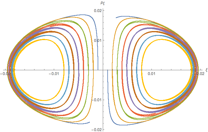
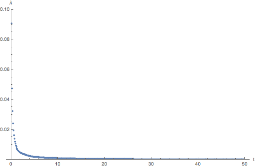
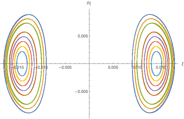
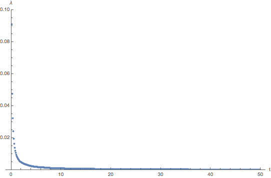
Figure 1: Numerical plots of the Poincaré sections (Left column) and Lyapunov exponents (Right column) for $\beta$-deformed ABJM. Here we set the energy of the string $E_{0}=0.01$. The top plots are for $\hat{\gamma}_{2}=\hat{\gamma}_{3}=0.01$ and the bottom plots are for $\hat{\gamma}_{2}=\hat{\gamma}_{3}=0.8$. The Poincaré sections are nicely foliated KAM tori and the Lyapunov exponent decays to zero for large time $t$, indicating non-chaotic dynamics of the string.

In order to obtain the corresponding Poincaré sections, we solve the Hamiltonian’s eoms (35a)-(35d) subjected to the constraints (4) and (B2). These are plotted in the left column of fig.1. The energy of the string is fixed at some particular value $E=E_{0}=0.01$, whereas the values of the YB deformation parameters are set as $\hat{\gamma}_{2}=\hat{\gamma}_{3}=0.01,\leavevmode\nobreak\ 0.8$. In addition, we choose the initial conditions as $\theta_{1}(0)=0$ and $p_{\xi}(0)=0$. Given this initial set of data, we generate a random data set for an interval $\xi(0)\in[0,1]$ which fixes the corresponding $p_{\theta_{1}}(0)$ in accordance with that of the constraint (4).

It is important to note that the other deformation parameter $\hat{\gamma}_{1}$ disappears from the numerical simulation since we switch off the $\quantity{\theta_{2},p_{\theta_{2}}}$ variables in the phase space. This is also visible form the Hamilton’s eoms (35a)-(35d), which do not depend on the choice of $\hat{\gamma}_{1}$.

We plot all these points on the $\{\xi,p_{\xi}\}$ plane every time the trajectories pass through $\theta_{1}=0$ hyper-plane. For the present example, the phase space under consideration is four dimensional, namely it is characterized by the coordinates $\{\theta_{1},p_{\theta_{1}},\xi,p_{\xi}\}$. Poincare sections in this case show regular patches indicating a foliation in the phase space (cf. left column of fig.1).

In order to calculate the Lyapunonv exponent ($\lambda$), we choose to work with the initial conditions $E=E_{0}=0.01$ together with $\{\theta_{1}(0)=0,\xi(0)=0.008,p_{\theta_{1}}(0)=0.009,p_{\xi}(0)=0\}$ which are consistent with (4). When $\hat{\gamma}_{2}=\hat{\gamma}_{3}=0.8$, the initial conditions are set to be $\{\theta_{1}(0)=0,\xi(0)=0.013,p_{\theta_{1}}(0)=0.007,p_{\xi}(0)=0\}$ while we keep the energy to be fixed at $E=E_{0}=0.01$. With this initial set of data, we study the dynamical evolution of two nearby orbits in the phase space those have an initial separation $\Delta X_{0}=10^{-7}$ (cf. (B1) ). In the process, we generate a zero Lyapunov exponent at large $t$ as shown in the right column of fig.1. This observation indeed exhibits a non-chaotic dynamics for the phase space and ensures the integrability of the system.

3.2 Noncommutative ABJM

Noncommutative ABJM corresponds to a gravity dual that is obtained by applying YB deformation to its AdS₄ subspace. The corresponding Abelian $r$-matrix is constructed using the momenta operators along AdS₄ . The resulting space-time metric is given by [44]

$$\begin{split}\differential s^{2}=&\hskip 2.84526pt\frac{1}{4}\left(r^{2}\left(-dt^{2}+\mathcal{M}\left(dx_{1}^{2}+dx_{2}^{2}\right)\right)+\frac{dr^{2}}{r^{2}}\right)+ds_{CP^{3}}^{2}\,,\\[7.0pt] \differential s^{2}_{CP^{3}}=&\hskip 2.84526pt\mathrm{d}\xi^{2}+\frac{1}{4}\cos^{2}{\xi}(\mathrm{d}\theta_{1}^{2}+\sin^{2}{\theta_{1}}\mathrm{d}\phi_{1}^{2})+\frac{1}{4}\sin^{2}{\xi}(\mathrm{d}\theta_{2}^{2}+\sin^{2}{\theta_{2}}\mathrm{d}\phi_{2}^{2})\\ &+\bigg{(}\frac{1}{2}\cos{\theta_{1}}\mathrm{d}\phi_{1}-\frac{1}{2}\cos{\theta_{2}}\mathrm{d}\phi_{2}+\mathrm{d}\psi\bigg{)}^{2}\sin^{2}{\xi}\cos^{2}{\xi}\,,\end{split}$$ (37)

which is accompanied by a NS-NS two form

$$B=\frac{\mu\mathcal{M}r^{4}}{4}dx^{1}\wedge dx^{2},\hskip 5.69054pt\mathcal{M}^{-1}=1+\frac{\mu^{2}r^{4}}{4}\,,$$ (38)

where $t$, $x_{1}$, $x_{2}$ and $r$ are the coordinates of $AdS_{4}$ background and $\mu$ is the YB deformation parameter. We set $r=1$ for the rest of our analysis.

In the next step, we consider the winding string ansatz of the form

$$t= \hskip 2.84526ptt(\tau),\quad\theta_{1}=\theta_{1}(\tau),\quad\theta_{2}=\theta_{2}(\tau),\quad\xi=\xi(\tau),\quad\phi_{1}=\alpha_{1}\tau+\alpha_{2}\sigma,\quad\phi_{2}=\alpha_{3}\tau+\alpha_{4}\sigma,$$

$$\psi= \hskip 2.84526pt\alpha_{5}\tau+\alpha_{6}\sigma,\quad x_{1}=\alpha_{7}\tau+\alpha_{8}\sigma,\quad x_{2}=\alpha_{9}\tau+\alpha_{10}\sigma\,.$$ (39)

In our analytical as well as numerical analyses we make the following choices of the parameters appearing in (3.2) :

$$\begin{split}\alpha_{2}&=\alpha_{4}=\alpha_{6}=\alpha_{8}=\alpha_{10}=1\,;\\ \alpha_{1}&=\alpha_{3}=\alpha_{5}=\alpha_{7}=\alpha_{9}=0\,.\end{split}$$ (40)

With the above choices of parameters, the contribution of the $B$-field in the Polyakov action (2) vanishes. Using (40) and (37), the string action (2) can be expressed as

$$\begin{split}L_{P}&=-\frac{1}{2}\left[\frac{1}{4}\dot{t}^{2}-\dot{\xi}^{2}-\frac{1}{4}\dot{\theta}_{1}^{2}\,\cos^{2}\xi-\frac{1}{4}\dot{\theta}_{2}^{2}\,\sin^{2}\xi+\frac{\mathcal{M}}{4}\quantity(\alpha_{8}^{2}+\alpha_{10}^{2})\right.\\[5.0pt] &\quad\left.+\frac{\alpha_{2}^{2}}{4}\cos^{2}\xi\quantity(\sin^{2}\theta_{1}+\cos^{2}\theta_{1}\sin^{2}\xi)+\frac{\alpha_{4}^{2}}{4}\sin^{2}\xi\quantity(\sin^{2}\theta_{2}+\cos^{2}\theta_{2}\cos^{2}\xi)\right.\\[5.0pt] &\quad\left.+\sin^{2}\xi\cos^{2}\xi\Big{\{}\alpha_{6}^{2}+\alpha_{2}\alpha_{6}\cos\theta_{1}-\alpha_{4}\alpha_{6}\cos\theta_{2}-\frac{1}{2}\alpha_{2}\alpha_{4}\cos\theta_{1}\cos\theta_{2}\Big{\}}\right]\;.\end{split}$$ (41)

3.2.1 Analytical results

The equations of motion corresponding to the non-isometry coordinates $\theta_{1}$, $\theta_{2}$ and $\xi$ can be computed from (41) as

$$\begin{split}&\ddot{\theta}_{1}-2\tan\xi\,\dot{\xi}\dot{\theta}_{1}+\alpha_{2}\sin\theta_{1}\Big{(}\alpha_{2}\cos^{2}\xi\cos\theta_{1}+\quantity(\alpha_{4}\cos\theta_{2}-2\alpha_{6})\sin^{2}\xi\Big{)}=0\,,\end{split}$$ (42a)

$$\begin{split}&\ddot{\theta}_{2}+2\cot\xi\,\dot{\xi}\dot{\theta}_{2}+\alpha_{4}\sin\theta_{2}\Big{(}\alpha_{4}\sin^{2}\xi\cos\theta_{2}+\quantity(\alpha_{2}\cos\theta_{1}+2\alpha_{6})\cos^{2}\xi\Big{)}=0\,,\end{split}$$ (42b)

$$\begin{split}&8\ddot{\xi}+\sin 2\xi\quantity(\dot{\theta}_{1}^{2}-\dot{\theta}_{2}^{2})+2\alpha_{6}^{2}\sin 4\xi-2\alpha_{4}\alpha_{6}\cos\theta_{2}\sin 4\xi\\ &-\alpha_{2}\cos\theta_{1}\sin 4\xi\quantity(\alpha_{4}\cos\theta_{2}-2\alpha_{6})+\alpha_{2}^{2}\quantity(-\sin^{2}\theta_{1}\sin 2\xi+\frac{1}{2}\cos^{2}\theta_{1}\sin 4\xi)\\ &+\alpha_{4}^{2}\quantity(\sin^{2}\theta_{2}\sin 2\xi+\frac{1}{2}\cos^{2}\theta_{2}\sin 4\xi)=0\,.\end{split}$$ (42c)

Next, following the same line of arguments as in the previous Section 3.1.1 (cf. eq.(18)), we may easily verify that the energy-momentum tensor satisfies the Virasoro consistency conditions

$$\begin{split}\partial_{\tau}T_{\tau\tau}&=\leavevmode\nobreak\ 0\,,\quad\text{on-shell}\,,\\[5.0pt] \partial_{\tau}T_{\tau\sigma}&=\leavevmode\nobreak\ 0\,,\quad\text{trivially}\,.\end{split}$$ (43)

The string configuration is described by the three equations of motion (42a)-(42c). In order to study this configuration systematically, we choose the following invariant plane in the phase space:

$$\theta_{2} \sim 0\,, \Pi_{\theta_{2}} \equiv\dot{\theta}_{2}\sim 0\,.$$ (44)

Notice that, the choice (44) automatically satisfies the $\theta_{2}$ eom (42b). The eoms corresponding to $\theta_{1}$ and $\xi$ then reduce to

$$\begin{split}&\ddot{\theta}_{1}-2\dot{\xi}\dot{\theta}_{1}\tan\xi+\alpha_{2}\sin\theta_{1}\quantity[\alpha_{2}\cos\theta_{1}\cos^{2}\xi+\sin^{2}\xi\quantity(\alpha_{4}-2\alpha_{6})]=0\,,\end{split}$$ (45a)

$$\begin{split}&8\ddot{\xi}+\sin 2\xi\,\dot{\theta}_{1}^{2}+\sin 4\xi\Big{[}2\alpha_{6}^{2}+\frac{\alpha_{4}^{2}}{2}-2\alpha_{4}\alpha_{6}-\alpha_{2}\cos\theta_{1}\quantity(\alpha_{4}-2\alpha_{6})\Big{]}\\ &\qquad\qquad+\alpha_{2}^{2}\Big{[}-\sin^{2}\theta_{1}\sin 2\xi+\frac{1}{2}\sin 4\xi\cos^{2}\theta_{1}\Big{]}=0\,.\end{split}$$ (45b)

In the next step, in order to utilize the Kovacic’s algorithm to the string configuration in the reduced phase-space described by (45a) and (45b), we make the choice

$$\theta_{1} \sim 0\,, \Pi_{\theta_{1}} \equiv\dot{\theta}_{1}\sim 0\,.$$ (46)

This choice satisfies (45a) trivially, and we are left with the following eom:

$$\ddot{\xi}+\mathcal{A}_{\text{NC}}\sin 4\xi=0\,,$$ (47)

where

$$\mathcal{A}_{\text{NC}}=\frac{1}{8}\quantity[2\alpha_{6}\quantity(\alpha_{6}-\alpha_{4})-\alpha_{2}\quantity(\alpha_{4}-2\alpha_{6})+\frac{1}{2}\quantity(\alpha_{2}^{2}+\alpha_{4}^{2})]\,.$$ (48)

We now consider small fluctuations ($\eta$) around the invariant plane $\theta_{1}$. This results the normal variational equation (NVE) of the form

$$\ddot{\eta}-2\dot{\bar{\xi}}\tan\bar{\xi}\;\dot{\eta}+\alpha_{2}\quantity[\alpha_{2}\cos^{2}\bar{\xi}+\quantity(\alpha_{4}-2\alpha_{6})\sin^{2}\bar{\xi}\,]\eta=0\,,$$ (49)

where $\bar{\xi}$ is the solution to (47).

In order to study the NVE (49), we introduce the variable $z$ such that

$$\cos\bar{\xi}=z\,.$$ (50)

With (50) we may recast the NVE (49) as

$$\begin{split}\eta^{\prime\prime}(z)+\quantity(\frac{f^{\prime}(z)}{2f(z)}+\frac{2}{z})\eta^{\prime}(z)+\frac{\alpha_{2}}{f(z)}\Big{(}\alpha_{2}z^{2}+\quantity(\alpha_{4}-2\alpha_{6})\quantity(1-z^{2})\Big{)}\eta(z)=0\,,\end{split}$$ (51)

where

$$f(z)=\dot{\bar{\xi}}^{2}\sin^{2}\bar{\xi}=\quantity(E+\frac{\mathcal{A}_{\text{NC}}}{2}\quantity(8z^{4}-8z^{2}+1))\quantity(1-z^{2})\,,$$ (52)

$E$ being the constant of integration equal to the energy of the string. We set $E=1$ in our analysis.

Next, we convert (51) into the Schrödinger form by using (A2). The resulting equation can be written as

$$\omega^{\prime}(z)+\omega^{2}(z)=\frac{2B^{\prime}(z)+B^{2}(z)-4A(z)}{4}\equiv\mathcal{V}_{\text{NC}}(z)\,,$$ (53)

where $\mathcal{V}_{\text{NC}}(z)$ is the Schrödinger potential and

$$\begin{split}A(z)&=\frac{\alpha_{2}}{f(z)}\Big{(}\alpha_{2}z^{2}+\quantity(\alpha_{4}-2\alpha_{6})\quantity(1-z^{2})\Big{)}\,,\end{split}$$ (54a)

$$\begin{split}B(z)&=\quantity(\frac{f^{\prime}(z)}{2f(z)}+\frac{2}{z})\,.\end{split}$$ (54b)

The Schrödinger potential $\mathcal{V}_{\text{NC}}(z)$ can be written as

$$\mathcal{V}_{\text{NC}}=\frac{\mathcal{N}_{\text{NC}}}{\mathcal{D}_{\text{NC}}}\,,$$ (55)

where

$$\begin{split}\mathcal{N}_{\text{NC}}&=12\quantity(z^{2}-2)+\mathcal{A}^{2}_{\text{NC}}\Big{[}-54+536z^{2}+16z^{4}\quantity(-147+263z^{2}-208z^{4}+60z^{6})\Big{]}\\ &\qquad+4\mathcal{A}_{\text{NC}}\Big{[}-30+187z^{2}-280z^{4}+120z^{6}+2\alpha_{2}\quantity(-1+9z^{2}-16z^{4}+8z^{6})\\ &\qquad\quad\quad\quad+16\alpha_{2}\quantity(z^{2}-1)\quantity(z^{2}\alpha_{2}-\quantity(z^{2}-1)\alpha_{4}-2\alpha_{6})\Big{]}\,,\end{split}$$ (56a)

$$\begin{split}\mathcal{D}_{\text{NC}}&=4\quantity(1-z^{2})^{2}\quantity(2+\quantity(1-8z^{2}+8z^{4})\mathcal{A}_{\text{NC}})^{2}\,.\end{split}$$ (56b)

In order to find the solution to (53), we now expand the potential $\mathcal{V}_{\text{NC}}$ for small values of $z$ following the same argument that was presented in the previous section 3.1. The resulting $\omega(z)$ equation may be written as

$$\begin{split}&\leavevmode\nobreak\ \omega^{\prime}(z)+\omega^{2}(z)\simeq\widetilde{C}_{2}\,,\end{split}$$ (57a)

$$\begin{split}&\leavevmode\nobreak\ \widetilde{C}_{2}=\leavevmode\nobreak\ -\frac{6+27\mathcal{A}_{\text{NC}}+4\alpha_{2}\quantity(\alpha_{4}-2\alpha_{6})}{2\quantity(2+\mathcal{A}_{\text{NC}})}\,.\end{split}$$

whose solution may be expressed as

$$\omega(z)=\sqrt{\widetilde{C}_{2}}\leavevmode\nobreak\ \tanh[\sqrt{\widetilde{C}_{2}}\leavevmode\nobreak\ \quantity(z+\mathsf{C}_{2})\Big{]}\,,$$ (58)

where $\mathsf{C}_{2}$ is an arbitrary constant.

Now the Schrödinger potential $\mathcal{V}_{\text{NC}}$ given by (55) has poles of order $2$ at

$$z=\pm 1\,,\quad z=\pm\frac{1}{2}\sqrt{2-\frac{\sqrt{2}\sqrt{\mathcal{A}_{\text{NC}}\quantity(\mathcal{A}_{\text{NC}}-2)}}{\mathcal{A}_{\text{NC}}}}\,,\quad z=\pm\frac{1}{2}\sqrt{2+\frac{\sqrt{2}\sqrt{\mathcal{A}_{\text{NC}}\quantity(\mathcal{A}_{\text{NC}}-2)}}{\mathcal{A}_{\text{NC}}}}\,.$$ (59)

On the other hand, the order at infinity of $\mathcal{V}_{\text{NC}}$ is determined to be $2$. These satisfy the criterion Cd.$(iii)$ of the Kovacic’s algorithm as discussed in Appendix A. Also, for small $z$ the solution (58) is indeed a polynomial of degree $1$. These information together ensure the analytic integrability of the system.

3.2.2 Numerical results

In order to numerically study the integrability of the string configuration, we use the ansatz (3.2) with the choice of parameters given by (40).

The resulting Hamilton’s equations of motion are obtained as

$$\begin{split}\dot{\theta_{1}}=&\hskip 2.84526pt4p_{\theta_{1}}\sec^{2}\xi\,,\end{split}$$ (60a)

$$\begin{split}\dot{\xi}=&\hskip 2.84526ptp_{\xi}\,,\end{split}$$ (60b)

$$\begin{split}\dot{p_{\theta_{1}}}=&\hskip 2.84526pt\frac{1}{2}\cos^{2}\xi\sin\theta_{1}\quantity(\sin^{2}\xi-\cos\theta_{1}\cos^{2}\xi)\,,\end{split}$$ (60c)

$$\begin{split}\dot{p_{\xi}}=&\hskip 2.84526pt\frac{1}{2}\quantity(\cos\xi\sin^{2}\theta_{1}\sin\xi-\cos^{4}\frac{\theta_{{}_{1}}}{2}\sin 4\xi-8p^{2}_{\theta_{1}}\sec^{2}\xi\tan\xi)\,,\end{split}$$ (60d)

where we set $\theta_{2}=p_{\theta_{2}}=0$ in the rest of our analysis.

For numerical simulation, we set the following values of the Yang-Baxter deformation parameter: $\mu=0.01$, $0.8$.

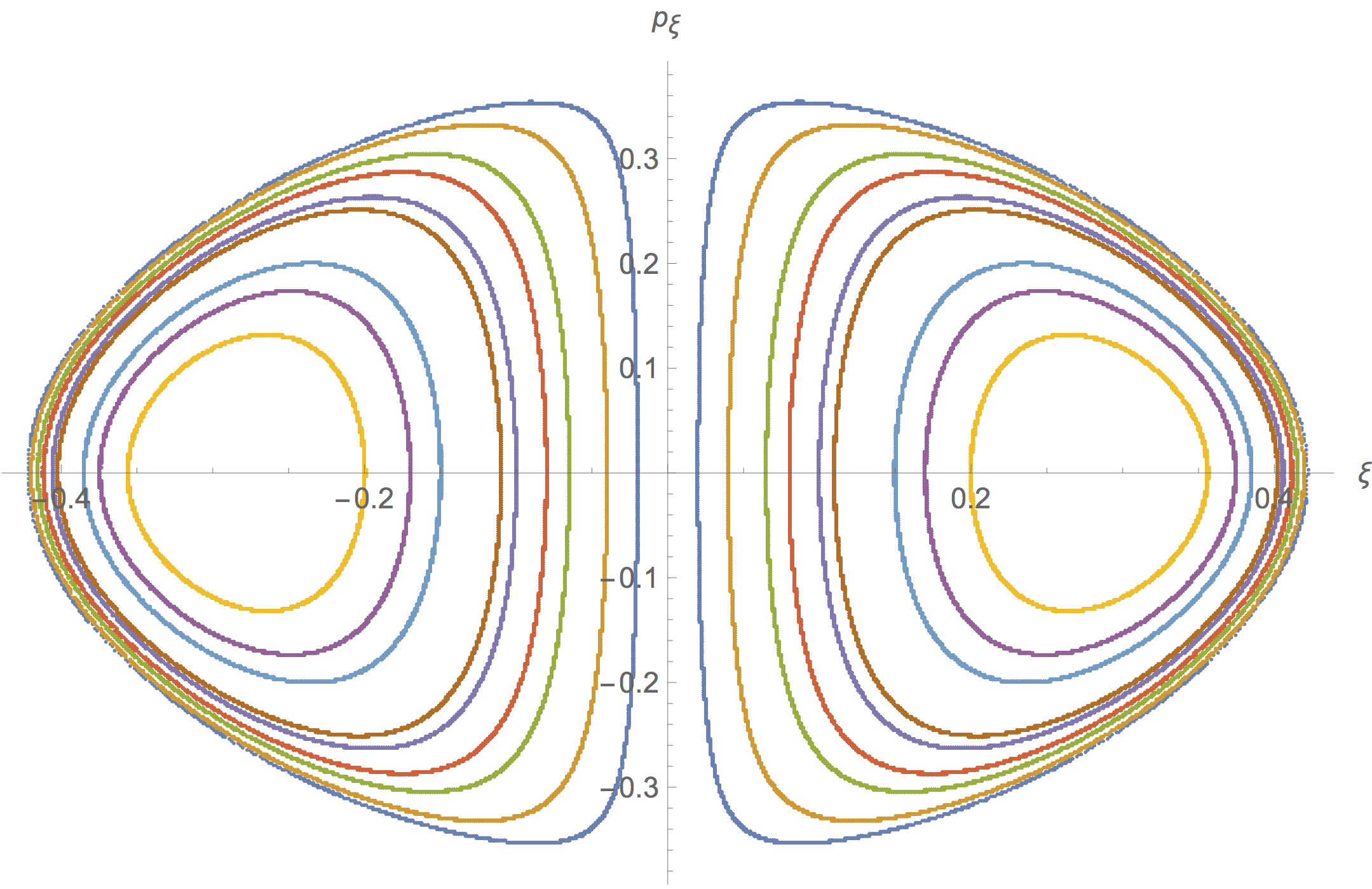
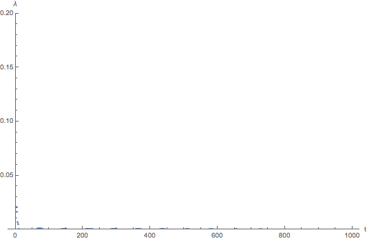
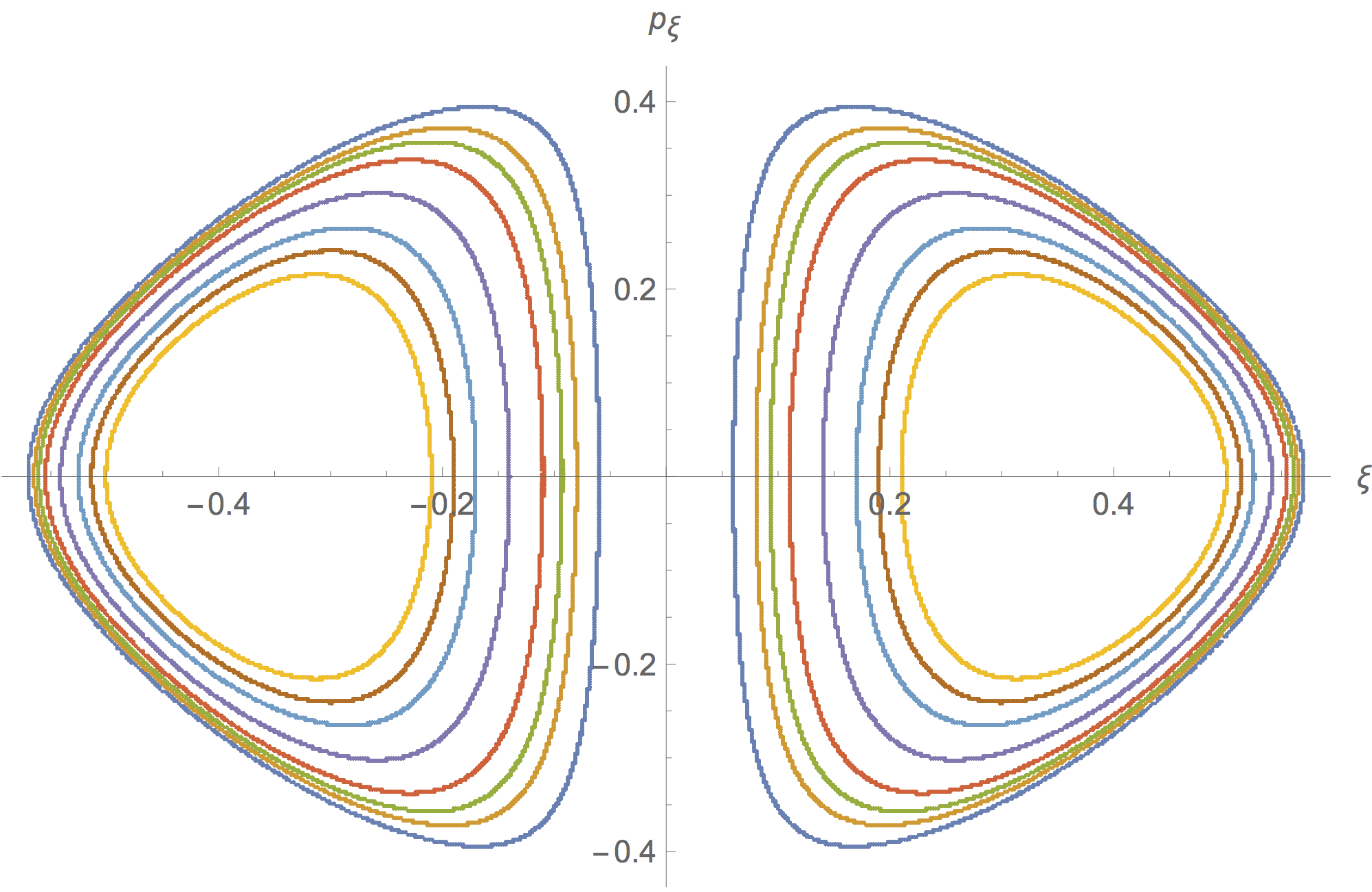
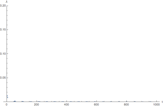
Figure 2: Numerical plots of the Poincaré sections (Left column) and Lyapunov exponents (Right column) for non-commutative ABJM. Here we set the energy of the string $E_{0}=0.4$. The top plots are for $\mu=0.01$ while the bottom plots are for $\mu=0.8$. The Poincaré sections are nicely foliated KAM tori in the phase space and the Lyapunov exponent decays to zero for large time $t$, indicating non-chaotic dynamics of the string.

Fig.2 shows the corresponding Poincaré sections when the energy of the string is $E=E_{0}=0.4$. Note that, we take the initial condition as $\theta_{1}(0)=0$, $p_{\xi}(0)=0$. We generate a random data set by choosing $\xi(0)\in[0,1]$ which fixes the initial momenta $p_{\theta_{1}}(0)$ following the Hamiltonian constraints (4) and (B2). The $\quantity{\xi,p_{\xi}}$ cross-section is obtained by collecting the data every time the trajectory passes through the $\theta_{1}=0$ plane.

In order to plot the Lyapunov exponent ($\lambda$) (fig.2), we set the initial conditions as $\{\theta_{1}(0)=0,\xi(0)=0.11,p_{\theta_{1}}(0)=0.17,p_{\xi}(0)=0\}$ together with $\Delta X_{0}=10^{-7}$ in (B1). For $\mu=0.8$ the initial conditions are changed to $\quantity{\theta_{1}(0)=0,\xi(0)=0.11,p_{\theta_{1}}(0)=0.22,p_{\xi}(0)=0}$. The energy of these orbits are fixed at $E=E_{0}=0.4$ such that, when put together, they satisfy the Hamiltonian constraints (4) and (B2). In the process, we finally generate a vanishing Lyapunov exponent at large time ($t$) exhibiting a non-chaotic motion.

3.3 Dipole deformed ABJM

Gravity dual of dipole deformed ABJM is obtained by considering a three parameter YB deformation of AdS₄ $\times$ CP³. The associated $r$-matrix is constructed combining the generators of both the AdS₄ and CP³ subspaces. The corresponding line element is given by [44]

$$\begin{split}\differential s^{2}=&\leavevmode\nobreak\ \frac{1}{4}\left(r^{2}\left(-\differential x_{0}^{2}+\differential x_{1}^{2}\right)+\frac{r^{2}}{1+f_{3}^{2}}\differential x_{2}^{2}+\frac{\differential r^{2}}{r^{2}}\right)+\differential\xi^{2}\\ &+\frac{1}{4}\cos^{2}\xi\left(\differential\theta_{1}^{2}+\sin^{2}\theta_{1}\differential\varphi_{1}^{2}\right)+\frac{1}{4}\sin^{2}\xi\left(\differential\theta_{2}^{2}+\sin^{2}\theta_{2}\differential\varphi_{2}^{2}\right)\\ &+\frac{1}{1+f_{3}^{2}}\left(\frac{1}{2}\cos\theta_{1}\differential\varphi_{1}-\frac{1}{2}\cos\theta_{2}\differential\varphi_{2}+\differential\psi\right)^{2}\sin^{2}\xi\cos^{2}\xi\,,\end{split}$$ (61)

together with the NS-NS fluxes

$$\begin{split}B=&-\frac{1}{4}\left(\frac{f_{3}}{1+f_{3}^{2}}\right)r\differential x_{2}\wedge\left(\frac{1}{2}\cos\theta_{1}\differential\varphi_{1}-\frac{1}{2}\cos\theta_{2}\differential\varphi_{2}+\differential\psi\right)\sin\xi\cos\xi\,,\\ f_{3}=&\frac{\mu r}{2}\sin(2\xi)\,.\end{split}$$ (62)

We also set the Yang-Baxter deformation parameters as $\mu_{1}=\mu_{2}=0,\mu_{3}=\mu$. Here, $\{r,x_{0},x_{1},x_{2}\}$ are the $AdS_{4}$ coordinates. On the other hand, $\{\xi,\theta_{1},\theta_{2},\varphi_{1},\varphi_{2},\psi\}$ are the coordinates of internal $CP^{3}$ manifold. In the following analysis, we choose $x_{0}=t$,$x_{1}=$ constant and $r=1$.

In our analysis, we choose to work with the winding string ansatz of the form

$$t= t(\tau),\quad\theta_{1}=\theta_{1}(\tau),\quad\theta_{2}=\theta_{2}(\tau),\quad\xi=\xi(\tau),\quad\varphi_{1}=\alpha_{1}\tau+\alpha_{2}\sigma,\quad$$

$$\varphi_{2}= \beta_{1}\tau+\beta_{2}\sigma,\quad\psi=\gamma_{1}\tau+\gamma_{2}\sigma,\quad x_{2}=\eta_{1}\tau+\eta_{2}\sigma\,,$$ (63)

with the following choices of the parameters:

$$\begin{split}\alpha_{1}&=\beta_{1}=\gamma_{1}=\eta_{1}=0\,,\\[5.0pt] \alpha_{2}&=\beta_{2}=\gamma_{2}=\eta_{2}=1\,.\end{split}$$ (64)

Using the above ansatz (3.3) we may write the Lagrangian in the action (2) as

$$\begin{split}L_{P}&=-\frac{1}{2}\Bigg{[}\frac{1}{4}\dot{t}^{2}-\dot{\xi}^{2}-\frac{1}{4}\dot{\theta}_{1}^{2}\cos^{2}\xi-\frac{1}{4}\dot{\theta}_{2}^{2}\sin^{2}\xi+\frac{\eta_{2}^{2}}{4\quantity(1+f_{3}^{2})}+\frac{\alpha_{2}^{2}\cos^{2}\xi}{4}\\ &\quad\times\quantity(\sin^{2}\theta_{1}+\frac{\sin^{2}\xi\cos^{2}\theta_{1}}{1+f_{3}^{2}})+\frac{\beta_{2}^{2}\sin^{2}\xi}{4}\quantity(\sin^{2}\theta_{2}+\frac{\cos^{2}\xi\cos^{2}\theta_{2}}{1+f_{3}^{2}})\\ &\quad+\frac{\sin^{2}\xi\cos^{2}\xi}{1+f_{3}^{2}}\Big{(}\gamma_{2}^{2}-\frac{1}{2}\alpha_{2}\beta_{2}\cos\theta_{1}\cos\theta_{2}+\alpha_{2}\gamma_{2}\cos\theta_{1}-\beta_{2}\gamma_{2}\cos\theta_{2}\Big{)}\Bigg{]}\,.\end{split}$$ (65)

3.3.1 Analytical results

The eoms resulting from the variations of $\theta_{1}$, $\theta_{2}$ and $\xi$ in (65) can be computed as

$$\begin{split}0=&\leavevmode\nobreak\ 4\quantity(1+\frac{\mu^{2}}{4}\sin^{2}2\xi)\quantity(\cos\xi\,\ddot{\theta}_{1}-2\sin\xi\,\dot{\xi}\,\dot{\theta}_{1})-4\alpha_{2}\cos\xi\sin^{2}\xi\quantity(2\gamma_{2}-\beta_{2}\cos\theta_{2})\sin\theta_{1}\\ &\leavevmode\nobreak\ +2\alpha_{2}^{2}\quantity(1+\mu^{2}\sin^{2}\xi)\cos^{3}\xi\sin 2\theta_{1}\,,\end{split}$$ (66a)

$$\begin{split}0=&\leavevmode\nobreak\ 2\quantity(1+\frac{\mu^{2}}{4}\sin^{2}2\xi)\quantity(\sin\xi\,\ddot{\theta}_{2}-2\cos\xi\,\dot{\xi}\,\dot{\theta}_{2})+2\beta_{2}\sin\xi\cos^{2}\xi\big{(}2\gamma_{2}+\alpha_{2}\cos\theta_{1}\\ &\leavevmode\nobreak\ -\beta_{2}\cos\theta_{2}\big{)}\sin\theta_{2}+\beta_{2}^{2}\quantity(1+\frac{\mu^{2}}{4}\sin^{2}2\xi)\sin\xi\sin 2\theta_{2}\,,\end{split}$$ (66b)

$$\begin{split}0=&\leavevmode\nobreak\ \quantity(1+\frac{\mu^{2}}{4}\sin^{2}2\xi)^{2}\quantity(16\ddot{\xi}+2\sin 2\xi\quantity(\dot{\theta}_{1}^{2}-\dot{\theta}_{2}^{2}-\beta_{2}^{2}\sin^{2}\theta_{2}-\alpha_{2}^{2}\sin^{2}\theta_{1}))\\ &\leavevmode\nobreak\ +\frac{\sin 4\xi}{2}\Big{(}4\gamma_{2}^{2}-\mu^{2}\eta_{2}^{2}+\alpha_{2}^{2}\cos^{2}\theta_{1}+\beta_{2}^{2}\cos^{2}\theta_{2}-4\beta_{2}\gamma_{2}\cos\theta_{2}\\ &\leavevmode\nobreak\ +2\alpha_{2}\cos\theta_{1}\quantity(2\gamma_{2}-\beta_{2}\cos\theta_{2})\Big{)}\,.\end{split}$$ (66c)

Now using the definition (5) of the energy-momentum tensor $T_{ab}$, it is easy to check that

$$\begin{split}\partial_{\tau}T_{\tau\tau}&=0\,,\quad\text{on-shell}\,,\\[4.0pt] \partial_{\tau}T_{\tau\sigma}&=0\,,\quad\text{trivially}\,.\end{split}$$ (67)

In the next step, we study the dynamics of the string governed by the eoms (66). In our analysis we first choose the $\theta_{2}$ invariant plane in the phase space defined as

$$\theta_{2}\sim 0\,\qquad\Pi_{\theta_{2}}:=\dot{\theta}_{2}\sim 0\,.$$ (68)

This choice trivially satisfies the $\theta_{2}$ eom (66b), and the remaining two eoms (66a), (66c) reduce to

$$\begin{split}0=&\leavevmode\nobreak\ 4\quantity(1+\frac{\mu^{2}}{4}\sin^{2}2\xi)\quantity(\cos\xi\,\ddot{\theta}_{1}-2\sin\xi\,\dot{\xi}\,\dot{\theta}_{1})-4\alpha_{2}\cos\xi\sin^{2}\xi\quantity(2\gamma_{2}-\beta_{2})\sin\theta_{1}\\ &\leavevmode\nobreak\ +2\alpha_{2}^{2}\quantity(1+\mu^{2}\sin^{2}\xi)\cos^{3}\xi\sin 2\theta_{1}\,,\end{split}$$ (69a)

$$\begin{split}0=&\leavevmode\nobreak\ \quantity(1+\frac{\mu^{2}}{4}\sin^{2}2\xi)^{2}\quantity(16\ddot{\xi}+2\sin 2\xi\quantity(\dot{\theta}_{1}^{2}-\alpha_{2}^{2}\sin^{2}\theta_{1}))\\ &\leavevmode\nobreak\ +\frac{\sin 4\xi}{2}\Big{(}4\gamma_{2}^{2}-\mu^{2}\eta_{2}^{2}+\alpha_{2}^{2}\cos^{2}\theta_{1}+\beta_{2}^{2}-4\beta_{2}\gamma_{2}+2\alpha_{2}\cos\theta_{1}\quantity(2\gamma_{2}-\beta_{2})\Big{)}\,.\end{split}$$ (69b)

The dynamics of the string in the reduced phase space, governed by (69a) and (69b), can be studied by further choosing the $\theta_{1}$ invariant plane defined as

$$\theta_{1}\sim 0\,,\qquad\Pi_{\theta_{1}}\equiv\dot{\theta}_{1}\sim 0\,.$$ (70)

While is choice trivially satisfies (69a), (69b) reduces to the form

$$16\quantity(1+\frac{\mu^{2}}{4}\sin^{2}2\xi)^{2}\ddot{\xi}+\quantity(\mathcal{A}_{\text{DD}}-\mu^{2}\eta_{2}^{2})\sin 4\xi=0\,,$$ (71)

where

$$\mathcal{A}_{\text{DD}}=\frac{1}{2}\Big{(}4\gamma_{2}^{2}+\alpha_{2}^{2}+\beta_{2}^{2}-4\beta_{2}\gamma_{2}+2\alpha_{2}\quantity(2\gamma_{2}-\beta_{2})\Big{)}\,.$$ (72)

Next we consider infinitesimal fluctuation ($\delta\theta_{1}\sim\eta$) around the $\theta_{1}$ invariant plane. This results in the normal variational equation (NVE) equation which can be written as

$$\begin{split}&\quantity(1+\frac{\mu^{2}}{4}\sin^{2}2\xi)\quantity(\cos\xi\,\ddot{\eta}-2\sin\xi\,\dot{\xi}\,\dot{\eta}_{1})\\ &\qquad\qquad+\Big{(}\alpha_{2}^{2}\quantity(1+\mu^{2}\sin^{2}\bar{\xi})\cos^{3}\bar{\xi}-\alpha_{2}\quantity(2\gamma_{2}-\beta_{2})\cos\bar{\xi}\sin^{2}\bar{\xi}\Big{)}\eta=\leavevmode\nobreak\ 0\,.\end{split}$$ (73)

Using the change in variable $\displaystyle\cos\bar{\xi}=z$ we may recast (73) in the form

$$\eta^{\prime\prime}(z)+B(z)\eta^{\prime}(z)+A(z)=0\,,$$ (74)

where

$$\begin{split}B(z)=&\leavevmode\nobreak\ \frac{f^{\prime}(z)}{2f(z)}+\frac{2}{z}\,,\end{split}$$ (75a)

$$\begin{split}A(z)=&\leavevmode\nobreak\ \frac{\alpha_{2}^{2}z^{2}\quantity(1+\mu^{2}\quantity(1-z^{2}))-\alpha_{2}\quantity(2\gamma_{2}-\beta_{2})\quantity(1-z^{2})}{\Big{(}1+\mu^{2}z^{2}\quantity(1-z^{2})\Big{)}f(z)}\,,\end{split}$$ (75b)

$$\begin{split}f(z)=&\leavevmode\nobreak\ \dot{\bar{\xi}}^{2}\sin^{2}\bar{\xi}\\ =&\leavevmode\nobreak\ \Bigg{(}E+\frac{\mathcal{A}_{\text{DD}}-\mu^{2}\eta_{2}^{2}}{32}\quantity(8z^{4}-8z^{2}+1)-\frac{\mu^{2}\mathcal{A}_{\text{DD}}}{128}\quantity(-128z^{8}+256z^{6}-152z^{4}+24z^{2})\Bigg{)}\\ &\leavevmode\nobreak\ \times\quantity(1-z^{2})\,.\end{split}$$ (75c)

In (75c) $E$ is the energy of the propagating string and we choose $E=1$ without any loss of generality. Also notice that, in deriving (75c) we series expand (71) for small values of the YB parameter $\mu$ and keep terms upto $\order{\mu^{2}}$.

We can further recast (74) in the Schrödinger form (A3) using (A2). The resulting equation can then be written as

$$\omega^{\prime}(z)+\omega^{2}(z)=\frac{2B^{\prime}(z)+B^{2}(z)-4A(z)}{4}\equiv\mathcal{V}_{\text{DD}}(z)\,,$$ (76)

where $\mathcal{V}_{\text{DD}}(z)$ is the Schrödinger potential whose exact form is quite complicated and we avoid writing the detailed expression here. However, we can expand this potential $\mathcal{V}_{\text{DD}}(z)$ for small $\mu$ as well as small $z$. The latter expansion is justified whenever we work with the full CP³ metric (61). The final form of (76) can be computed as

$$\omega^{\prime}(z)+\omega^{2}(z)\approx\widetilde{C}_{3}\,,$$ (77)

where

$$\begin{split}\widetilde{C}_{3}=&\leavevmode\nobreak\ -\frac{96+27\mathcal{A}_{\text{DD}}+64\alpha_{2}\beta_{2}-128\alpha_{2}\gamma_{2}}{2\quantity(32+\mathcal{A}_{\text{DD}})}\\ &\leavevmode\nobreak\ +\frac{\quantity(-288\mathcal{A}_{\text{DD}}-9\mathcal{A}_{\text{DD}}^{2}+384\eta_{2}^{2}-32\alpha_{2}\beta_{2}\eta_{2}^{2}+64\alpha_{2}\gamma_{2}\eta_{2}^{2})\mu^{2}}{\quantity(32+\mathcal{A}_{\text{DD}})^{2}}+\order{\mu^{4}}\,.\end{split}$$ (78)

The general solution to (77) may be obtained as

$$\omega(z)=\sqrt{\widetilde{C}_{3}}\leavevmode\nobreak\ \tanh\quantity(\sqrt{\widetilde{C}_{3}}\leavevmode\nobreak\ \quantity(z+\mathsf{C}_{3}))\,,$$ (79)

where $\mathsf{C}_{3}$ is the integration constant. Note that, for small $z$ the solution (79) is indeed a polynomial of degree $1$. Moreover, there are poles of order $2$ of the potential $\mathcal{V}_{\text{DD}}(z)$ at

$$z=\pm 1\,,\qquad z=z_{i}\,\quad i=1,\cdots,4\,,$$ (80)

and the order at infinity of $\mathcal{V}_{\text{DD}}(z)$ is $2$. Thus the criterion Cd(iii) of the Kovacic’s algorithm, discussed in Appendix A, is satisfied. From these results we can infer that the system is indeed integrable.

3.3.2 Numerical results

We now explore the non-chaotic dynamics of the string configuration using numerical methods. In order to do so, we note down the corresponding Hamilton’s equations of motion

$$\begin{split}\dot{\theta_{1}}=&\hskip 2.84526pt4p_{\theta_{1}}\sec^{2}\xi\,,\end{split}$$ (81a)

$$\begin{split}\dot{\xi}=&\hskip 2.84526ptp_{\xi}\,,\end{split}$$ (81b)

$$\begin{split}\dot{p_{\theta_{1}}}=&\hskip 2.84526pt\frac{\cos^{4}\xi(-2-\mu^{2}+\mu^{2}\cos(2\xi))\sin(2\theta_{1})+\sin\theta_{1}\sin^{2}(2\xi)}{8+2\mu^{2}\sin^{2}(2\xi)}\,,\end{split}$$ (81c)

$$\begin{split}\dot{p_{\xi}}=&\hskip 2.84526pt\frac{\mathcal{N}_{2}}{8(4+\mu^{2}\sin^{2}(2\xi))^{2}}\,,\end{split}$$ (81d)

where we denote

$$\mathcal{N}_{2}= \hskip 2.84526pt\bigg{(}-32\big{(}3-2\mu^{2}+4\cos\theta_{1}+\cos{(2\theta_{1})}\big{)}\cos(2\xi)-8\big{(}8+\mu^{2}-\mu^{2}\cos(4\xi)\big{)}^{2}p^{2}_{\theta_{1}}\sec^{4}\xi$$

$$+\big{(}8+\mu^{2}-\mu^{2}\cos(4\xi)\big{)}^{2}\sin^{2}\theta_{1}\bigg{)}\cos\xi\sin\xi.$$ (82)

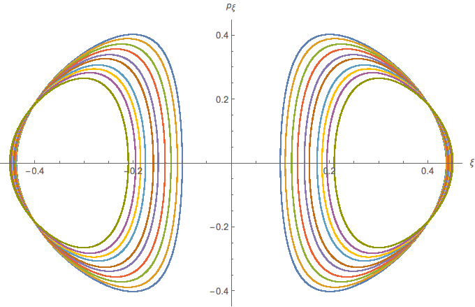
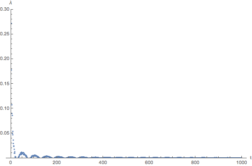
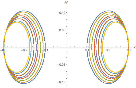
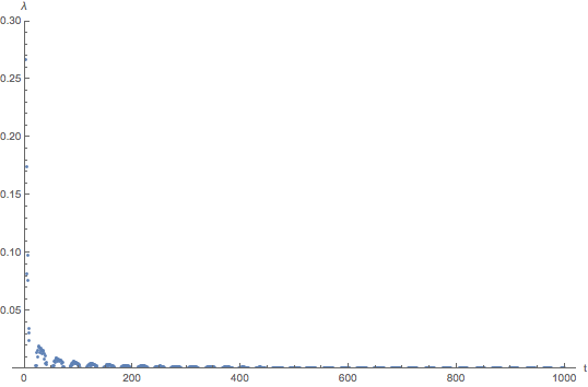
Figure 3: Numerical plots of the Poincaré sections (Left column) and Lyapunov exponents (Right column) for dipole deformed ABJM. Here we set the energy of the string $E_{0}=0.35$. The top plots are for $\mu=0.01$ while the bottom plots are for $\mu=0.8$. The Poincaré sections can be seen to be undistorted foliations of KAM tori in the phase space and for large time $t$ the Lyapunov exponent decays to zero. These are indications of the non-chaotic dynamics of the string configuration.

In order to obtain the Poincaré sections, we set the energy as $E=E_{0}=0.35$ while the rest of the data is chosen as $\theta_{1}(0)=0$ and $p_{\xi}(0)=0$. Given this initial data, we generate a random data set for $p_{\theta_{1}}(0)$ by choosing $\xi(0)\in[0,1]$ such that the constraints (B2) are satisfied. We also set the values of the parameters as in (64).

In our numerical analysis, the YB parameter is set to be, $\mu=0.01$ and $0.8$. As in the previous cases, the Poincaré sections (Fig.3) are obtained by plotting all the points those are on the $\{\xi,p_{\xi}\}$ plane which correspond to trajectories passing through the $\theta_{1}=0$ hyper-plane.

In order to calculate the Lyapunov exponent ($\lambda$), we set the initial conditions as $\theta_{1}(0)=0$, $p_{\xi}(0)=0$, $\xi(0)=0.1$ and $p_{\theta_{1}}(0)=0.23$ those are compatible with the Hamiltonian constraint (B2). The initial separation between the two nearby trajectories is set to be $\Delta X_{0}=10^{-7}$ as before, which eventually results in a zero value for the Lyapunov (Fig.3) for large $t$. For YB parameter value $\mu=0.8$, the initial data are set to be $\theta_{1}(0)=0$, $p_{\xi}(0)=0$, $\xi(0)=0.2$ and $p_{\theta_{1}}(0)=0.22$.

Clearly, the nicely foliated KAM tori trajectories in the phase space along with the vanishing Lyapunov exponent indicate non-chaotic dynamics of the superstring propagating in this deformed background.

3.4 Nonrelativistic ABJM

The gravity dual of nonrelativistic ABJM is obtained by constructing Abelian $r$-matrices using Cartan generators of both AdS₄ as well as CP³ subspaces. The corresponding line element is given by [44]

$$\begin{split}\differential s^{2}=&\frac{1}{4}\left(-2r^{2}dx_{+}dx_{-}+r^{2}dx_{1}^{2}+\frac{dr^{2}}{r^{2}}-\mathcal{M}r^{2}dx_{+}^{2}\right)+\differential s_{CP^{3}}^{2}\,,\\[5.0pt] \mathrm{d}s^{2}_{CP^{3}}=&\hskip 2.84526pt\mathrm{d}\xi^{2}+\frac{1}{4}\cos^{2}{\xi}(\mathrm{d}\theta_{1}^{2}+\sin^{2}{\theta_{1}}\mathrm{d}\phi_{1}^{2})+\frac{1}{4}\sin^{2}{\xi}(\mathrm{d}\theta_{2}^{2}+\sin^{2}{\theta_{2}}\mathrm{d}\phi_{2}^{2})\\ &\quad+\bigg{(}\frac{1}{2}\cos{\theta_{1}}\mathrm{d}\phi_{1}-\frac{1}{2}\cos{\theta_{2}}\mathrm{d}\phi_{2}+\mathrm{d}\psi\bigg{)}^{2}\sin^{2}{\xi}\cos^{2}{\xi}\,,\end{split}$$ (83)

where

$$\begin{split}\mathcal{M}&=f_{1}^{2}+f_{2}^{2}+f_{3}^{2}\,,\\ f_{1}&=\frac{r}{2\sqrt{2}}\mu_{1}\sin\theta_{1}\cos\xi\,,\\ f_{2}&=\frac{r}{2\sqrt{2}}\mu_{2}\sin\theta_{2}\sin\xi\,,\\ f_{3}&=\frac{r}{2\sqrt{2}}\left(2\mu_{3}-\mu_{1}\cos\theta_{1}+\mu_{2}\cos\theta_{2}\right)\sin\xi\cos\xi\,.\end{split}$$ (84)

The corresponding $B$-field may be written as

$$\begin{split}B=&-\frac{1}{\sqrt{2}}r\cos\xi\left(f_{1}\sin\theta_{1}-f_{3}\cos\theta_{1}\sin\xi\right)dx_{+}\wedge d\varphi_{1}\\ &-\frac{1}{\sqrt{2}}r\sin\xi\left(f_{3}\cos\theta_{2}\cos\xi+f_{2}\sin\theta_{2}\right)dx_{+}\wedge d\varphi_{2}\\ &+\frac{1}{\sqrt{2}}r\sin(2\xi)f_{3}dx_{+}\wedge d\psi\,.\end{split}$$ (85)

The light-cone coordinates $x_{\pm}$ appearing in (83) and (85) are given by

$$x_{\pm}=\frac{1}{\sqrt{2}}\left(x^{0}\pm x^{2}\right)\,.$$ (86)

Notice that, in (83) $\mu_{i}$ $(i=1,2,3)$ are the Yang-Baxter (YB) deformation parameters of the theory. Also, the metric (83) corresponds to a Schrödinger space-time with dynamical critical exponent $2$. In the following analytical and numerical analyses, we choose the AdS₄ coordinates as $x_{0}=t$, $r=1$ and $x_{1}=$constant.

We now work with the winding string ansatz of the form

$$x_{+} =\leavevmode\nobreak\ x_{+}(\tau)\,, \theta_{1} =\theta_{1}(\tau)\,, \theta_{2} =\theta_{2}(\tau)\,, \xi =\xi(\tau)\,,$$ (87)

$$\phi_{1} =\alpha_{1}\tau+\alpha_{2}\sigma\,, \phi_{2} =\alpha_{3}\tau+\alpha_{4}\sigma\,, \psi =\alpha_{5}\tau+\alpha_{6}\sigma\,, x_{-} =\eta_{1}\tau+\eta_{2}\sigma\,.$$

However, in order to further simplify our analysis we choose of the parameters $\alpha_{i}$ $(i=1,\cdots,6)$ and $\eta_{j}$ $(j=1,2)$ appearing in (87) as

$$\begin{split}\alpha_{1}&=\alpha_{3}=\alpha_{5}=\eta_{2}=\leavevmode\nobreak\ 0\,,\\ \alpha_{2}&=\alpha_{4}=\alpha_{6}=\eta_{1}=\leavevmode\nobreak\ 1\,.\end{split}$$ (88)

Using (87) and (88), the Lagrangian in the Polyakov action (2) can be written as

$$\begin{split}L_{P}&=-\frac{1}{2}\Bigg{[}\frac{\mathcal{M}}{4}\dot{x}_{+}^{2}-\dot{\xi}^{2}-\frac{1}{4}\quantity(\dot{\theta}_{1}^{2}\cos^{2}\xi+\dot{\theta}_{2}^{2}\sin^{2}\xi)+\frac{\alpha_{2}^{2}}{4}\cos^{2}\xi\quantity(\sin^{2}\theta_{1}+\sin^{2}\xi\cos^{2}\theta_{1})\\ &\quad+\frac{\alpha_{4}^{2}}{4}\sin^{2}\xi\quantity(\sin^{2}\theta_{2}+\cos^{2}\xi\cos^{2}\theta_{2})+\sin^{2}\xi\cos^{2}\xi\Big{(}\alpha_{6}^{2}+\alpha_{2}\alpha_{6}\cos\theta_{1}-\alpha_{4}\alpha_{6}\cos\theta_{2}\\ &\quad-\frac{1}{2}\alpha_{2}\alpha_{4}\cos\theta_{1}\cos\theta_{2}\Big{)}\Bigg{]}-\frac{\alpha_{2}}{\sqrt{2}}\cos\xi\quantity(f_{1}\sin\theta_{1}-f_{3}\sin\xi\cos\theta_{1})\\ &\quad-\frac{\alpha_{4}}{\sqrt{2}}\sin\xi\quantity(f_{2}\sin\theta_{2}+f_{3}\cos\xi\cos\theta_{2})+\frac{\alpha_{6}}{\sqrt{2}}f_{3}\sin 2\xi\,.\end{split}$$ (89)

Notice that, although we choose the parameters $\alpha_{i}$ $(i=1,\cdots,8)$ as given by (88), there exists a non-trivial contribution of the $B$-field in the dynamics of the string unlike the previous cases in Sections 3.1, 3.2 and 3.3, respectively.

3.4.1 Analytical results

We first use (89) to derive the eoms corresponding to the $\theta_{1}$, $\theta_{2}$ and $\xi$ coordinates. The results are written as

$$\begin{split}0=&\leavevmode\nobreak\ 8\cos\xi\leavevmode\nobreak\ \ddot{\theta}_{1}-16\sin\xi\leavevmode\nobreak\ \dot{\xi}\dot{\theta}_{1}-\sin^{2}\xi\cos\xi\sin\theta_{1}\Big{(}16\mu_{1}\alpha_{6}-8\mu_{1}\alpha_{2}\cos\theta_{1}+8\mu_{1}\alpha_{4}\cos\theta_{2}\\ &\leavevmode\nobreak\ -\quantity(\mu_{1}+8\alpha_{2})\quantity(-2\mu_{3}+\mu_{1}\cos\theta_{1}-\mu_{2}\cos\theta_{2})+8\quantity(-2\alpha_{2}\alpha_{6}+\alpha_{2}\alpha_{4}\cos\theta_{2})\Big{)}\\ &\leavevmode\nobreak\ +\cos\xi\sin 2\theta_{1}\quantity(8\mu_{1}\alpha_{2}+4\alpha_{2}^{2}\cos^{2}\xi+\mu_{1}^{2}\big{/}2)\,,\end{split}$$ (90a)

$$\begin{split}0=&\leavevmode\nobreak\ 8\sin\xi\leavevmode\nobreak\ \ddot{\theta}_{2}+16\cos\xi\leavevmode\nobreak\ \dot{\xi}\dot{\theta}_{2}+\sin\xi\cos^{2}\xi\sin\theta_{2}\Big{(}16\mu_{2}\alpha_{6}-8\mu_{2}\alpha_{4}\cos\theta_{2}+8\mu_{2}\alpha_{2}\cos\theta_{1}\\ &\leavevmode\nobreak\ -\quantity(\mu_{2}+8\alpha_{4})\quantity(2\mu_{3}-\mu_{1}\cos\theta_{1}+\mu_{2}\cos\theta_{2})-8\quantity(-2\alpha_{4}\alpha_{6}-\alpha_{2}\alpha_{4}\cos\theta_{1})\Big{)}\\ &\leavevmode\nobreak\ +\sin\xi\sin 2\theta_{2}\quantity(8\mu_{2}\alpha_{4}+4\alpha_{4}^{2}\sin^{2}\xi+\mu_{2}^{2}\big{/}2)\,,\end{split}$$ (90b)

$$\begin{split}0=&\leavevmode\nobreak\ \ddot{\xi}+\sin 2\xi\quantity(\dot{\theta}_{1}^{2}-\dot{\theta}_{2}^{2})+T_{\xi}\,,\end{split}$$ (90c)

where

$$\begin{split}T_{\xi}=&\leavevmode\nobreak\ 2\quantity(2\mu_{3}-\mu_{1}\cos\theta_{1}+\mu_{2}\cos\theta_{2})\Big{(}-1-\frac{\alpha_{6}}{2}-\frac{\alpha_{2}}{2}\cos\theta_{1}+\frac{\alpha_{4}}{2}\cos\theta_{2}\\ &\leavevmode\nobreak\ +\quantity(2\mu_{3}-\mu_{1}\cos\theta_{1}+\mu_{2}\cos\theta_{2})\big{/}32\Big{)}\sin 4\xi+2\sin 4\xi\leavevmode\nobreak\ \Big{(}\alpha_{6}^{2}-\alpha_{4}\alpha_{6}\cos\theta_{2}\\ &\leavevmode\nobreak\ -\frac{1}{2}\cos\theta_{1}\quantity(-2\alpha_{2}\alpha_{6}+\alpha_{2}\alpha_{4}\cos\theta_{2})\Big{)}+\sin 2\xi\leavevmode\nobreak\ \Bigg{\{}\frac{1}{2}\Big{(}\alpha_{2}^{2}\cos^{2}\theta_{1}\cos^{2}\xi-\alpha_{4}^{2}\cos^{2}\theta_{2}\sin^{2}\xi\Big{)}\\ &\leavevmode\nobreak\ -\frac{1}{16}\quantity(\mu_{1}^{2}\sin^{2}\theta_{1}-\mu_{2}^{2}\sin^{2}\theta_{2})-\quantity(\mu_{1}\alpha_{2}\sin^{2}\theta_{1}-\mu_{2}\alpha_{4}\sin^{2}\theta_{2})\\ &\leavevmode\nobreak\ -\frac{\alpha_{2}^{2}}{2}\Big{(}\sin^{2}\theta_{1}+\sin^{2}\xi\cos^{2}\theta_{1}\Big{)}+\frac{\alpha_{4}^{2}}{2}\Big{(}\sin^{2}\theta_{2}+\cos^{2}\xi\cos^{2}\theta_{2}\Big{)}\Bigg{\}}\,.\end{split}$$ (91)

On the other hand, the eom corresponding to the coordinate $x_{+}$ can be written as

$$\mathcal{M}\frac{\differential}{\differential\tau}\dot{x}_{+}+\dot{x}_{+}\frac{\differential}{\differential\tau}\mathcal{M}=\leavevmode\nobreak\ 0\,.$$ (92)

We can get rid of the first term in the LHS of (92) by choosing

$$x_{+}=\mathscr{E}\tau\,.$$ (93)

We can always set $\mathscr{E}=1$ without loss of any generality. Eq.(93) shows that $x_{+}$ is indeed the world-sheet time. However, the vanishing of the second term in the LHS of (92) results in the following constraint equation:

$$\begin{split}&\dot{\xi}\Big{[}\quantity(\mu_{2}^{2}\sin^{2}\theta_{2}-\mu_{1}^{2}\sin^{2}\theta_{1})\sin 2\xi+\quantity(2\mu_{3}-\mu_{1}\cos\theta_{1}+\mu_{2}\cos\theta_{2})^{2}\cos 2\xi\Big{]}\\ &+\dot{\theta}_{1}\Big{[}\mu_{1}^{2}\sin 2\theta_{1}\cos^{2}\xi+\mu_{1}\sin\theta_{1}\quantity(2\mu_{3}-\mu_{1}\cos\theta_{1}+\mu_{2}\cos\theta_{2})\sin 2\xi\Big{]}\\ &+\dot{\theta}_{2}\Big{[}\mu_{2}^{2}\sin 2\theta_{2}\sin^{2}\xi-\mu_{2}\sin\theta_{2}\quantity(2\mu_{3}-\mu_{1}\cos\theta_{1}+\mu_{2}\cos\theta_{2})\sin 2\xi\Big{]}=\leavevmode\nobreak\ 0\,.\end{split}$$ (94)

We may now compute the energy-momentum tensors using the definition (5). It is easy to check that

$$\partial_{\tau}T_{\tau\tau} =\mathcal{R}\,,$$ (95)

$$\partial_{\tau}T_{\tau\sigma} =0\,,$$ (96)

where

$$\begin{split}\mathcal{R}=&\leavevmode\nobreak\ \frac{\mu}{64}\Bigg{[}-\cos^{2}\xi\sin\theta_{1}\leavevmode\nobreak\ \dot{\theta}_{1}\Big{\{}4\mu+2\quantity(\mu-4)\cos\theta_{1}-4\mu\cos 2\xi\\ &\leavevmode\nobreak\ -\quantity(4-\mu)\Big{(}\cos\quantity(\theta_{1}-2\xi)+\cos\quantity(\theta_{1}+2\xi)-\cos\quantity(\theta_{2}-2\xi)-\cos\quantity(\theta_{2}+2\xi)\Big{)}\Big{\}}\\ &\leavevmode\nobreak\ +\sin^{2}\xi\leavevmode\nobreak\ \dot{\theta}_{2}\Big{\{}-4\quantity(-2\mu+\quantity(\mu-4)\cos\theta_{1}+4\cos\theta_{2})\cos^{2}\xi\sin\theta_{2}\\ &\leavevmode\nobreak\ -2\sin 2\theta_{2}\quantity(-4+\mu\sin^{2}\xi)\Big{\}}-\sin\xi\cos\xi\leavevmode\nobreak\ \dot{\xi}\Big{\{}2\quantity(\mu-4)\quantity(\cos 2\theta_{1}-\cos 2\theta_{2})\\ &\leavevmode\nobreak\ +4\quantity(-2+\cos\theta_{1}-\cos\theta_{2})\Big{(}-2\quantity(\mu+4)+\quantity(\mu-4)\quantity(\cos\theta_{1}-\cos\theta_{2})\Big{)}\cos 2\xi\Big{\}}\Bigg{]}\,.\end{split}$$ (97)

However, the Virasoro consistency conditions $\displaystyle\partial_{\tau}T_{ab}=0$ require us to set $\mathcal{R}=0$ in (97). Using this latter requirement and (94) we may now solve for $\dot{\xi}$ algebraically and substitute the resulting solution into the eoms (90a) and (90b) corresponding to $\theta_{1}$ and $\theta_{2}$, respectively. The resulting eoms are obvious and we avoid writing them here. Moreover, if we choose the $\theta_{2}$ invariant plane in the phase space described as

$$\theta_{2}\sim 0\,,\qquad\Pi_{\theta_{2}}:=\dot{\theta}_{2}\sim 0\,,$$ (98)

then we observe that the resulting $\theta_{2}$ eom (90b) (after $\dot{\xi}$ substitution) is satisfied trivially. The other two $\dot{\xi}$ substituted eoms (90a) and (90c) then reduce to

$$\begin{split}0=&\leavevmode\nobreak\ 8\cos\xi\leavevmode\nobreak\ \ddot{\theta}_{1}+8\sin 2\xi\sin\theta_{1}\leavevmode\nobreak\ \dot{\theta_{1}}^{2}\leavevmode\nobreak\ \mathscr{K}_{\theta_{1}}+\cos\xi\sin 2\theta_{1}\quantity(8\mu+4\cos^{2}\xi+\frac{\mu^{2}}{2})\\ &\leavevmode\nobreak\ -\cos\xi\sin^{2}\xi\sin 2\theta_{1}\Big{(}8\mu\quantity(\cos\theta_{1}+2)+8\quantity(1-\mu)+\mu\quantity(-3+\cos\theta_{1})\quantity(\mu+8)\Big{)}\,,\end{split}$$ (99a)

$$\begin{split}0=&\leavevmode\nobreak\ 4\ddot{\xi}+\frac{1}{2}\sin 2\xi\,\dot{\theta}_{1}^{2}+\mathscr{T}_{\xi}\,,\end{split}$$ (99b)

where

$$\begin{split}\mathscr{K}_{\theta_{1}}&=\leavevmode\nobreak\ -\frac{\quantity(16+6\mu)\quantity(1-\cos 2\xi)+2\quantity(\mu+8)\cos\theta_{1}+2\quantity(\mu+8)\cos\theta_{1}\cos 2\xi)}{2\sin\xi\Big{(}\quantity(\mu+8)\quantity(\cos 2\theta_{1}-1)+2\cos 2\xi\quantity(-3+\cos\theta_{1})\quantity(8-3\mu+\quantity(\mu+8)\cos 2\xi)\Big{)}}\\ &\leavevmode\nobreak\ +\frac{\quantity(3+\cos\theta_{1}\cot^{2}\xi)\sin\xi}{\sin^{2}\theta_{1}\quantity(3-\cos\theta_{1})^{2}\cos 2\xi}\,,\end{split}$$ (100)

$$\begin{split}\mathscr{T}_{\xi}=&\leavevmode\nobreak\ \frac{\mu}{2}\quantity(-3+\cos\theta_{1})\sin 4\xi+\cos^{2}\theta_{1}\sin\xi\cos^{3}\xi\\ &\leavevmode\nobreak\ +2\mu\Big{(}2+\quantity(-3+\cos\theta_{1})\Big{)}\cos\theta_{1}\sin\xi\cos^{3}\xi\\ &\leavevmode\nobreak\ +\quantity(\frac{\mu^{2}}{8}\quantity(-3+\cos\theta_{1})^{2}+1)\cos^{3}\xi\sin\xi-\mu\sin^{2}\theta_{1}\sin 2\xi\\ &\leavevmode\nobreak\ -\frac{1}{8}\cos\xi\Big{\{}\quantity(8+\mu^{2})\sin^{2}\theta_{1}\sin\xi+\sin^{3}\xi\Big{(}8+9\mu^{2}-2\quantity(-8+24\mu+3\mu^{2})\cos\theta_{1}\\ &\leavevmode\nobreak\ +\quantity(8+16\mu+\mu^{2})\cos^{2}\theta_{1}\Big{)}\Big{\}}\,.\end{split}$$ (101)

In the next step, we make the following choice of the $\theta_{1}$ invariant plane in the phase space:

$$\theta_{1}\sim 0\,,\qquad\Pi_{\theta_{1}}:=\dot{\theta}_{1}\sim 0\,,$$ (102)

which clearly satisfies (99a). Subsequently, the $\xi$ eom (99b) can be written in the form

$$\ddot{\xi}+\mathcal{A}_{\text{NR}}\sin 4\xi=0\,,$$ (103)

where

$$\begin{split}\mathcal{A}_{\text{NR}}=\frac{8-16\mu+\mu^{2}}{32}\,.\end{split}$$ (104)

Now from (94) and (97) we notice that, for the successive choices of the invariant planes in the phase space, namely (98) and (102), $\dot{\xi}=0$. Moreover, this solution must be consistent with (103). Since $\displaystyle 0\leq\xi<\pi$, the possible solutions of (103) can be expressed as

$$\bar{\xi}=\leavevmode\nobreak\ \frac{n\pi}{4}\,,\quad 0\leq n<4\,,n\in\mathbb{Z}\,.$$ (105)

We now consider infinitesimal fluctuations ($\delta\theta_{1}\sim\eta$) around the $\theta_{1}$ invariant plane. The resulting NVE can then be written as

$$\begin{split}\ddot{\eta}-\frac{1}{8}\Big{(}2\sin^{2}\bar{\xi}\quantity(4-\mu^{2})-8\cos^{2}\bar{\xi}-16\mu-\mu^{2}\Big{)}\eta\approx\leavevmode\nobreak\ 0\,,\end{split}$$ (106)

where $\bar{\xi}$ is given by (105). Also notice that, in writing the above NVE (106), we have neglected the second term in the R.H.S of (99a) since this term is $\order{\eta^{3}}$.

Next, with the given solutions (105), (106) can easily be solved. The solutions can formally be written as

$$\eta(\tau)=\leavevmode\nobreak\ \mathsf{C}_{1}\cos\quantity(\sqrt{\mathsf{C}_{0}}\leavevmode\nobreak\ \tau)+\mathsf{C}_{2}\sin\quantity(\sqrt{\mathsf{C}_{0}}\leavevmode\nobreak\ \tau)\,,$$ (107)

where

$$\mathsf{C}_{0}=\begin{cases}\frac{1}{8}\quantity(\mu^{2}+16\mu+8)\,,&\text{for $n=0$}\\[3.0pt] \frac{1}{4}\quantity(\mu^{2}+8\mu)\,,&\text{for $n=1$}\\[3.0pt] \frac{1}{8}\quantity(3\mu^{2}+16\mu-8)\,,&\text{for $n=2$}\\[3.0pt] \frac{1}{4}\quantity(\mu^{2}+8\mu)\,,&\text{for $n=3$}\,,\end{cases}$$ (108)

and $\mathsf{C}_{1}$ and $\mathsf{C}_{2}$ are constants of integration.

Clearly, these solutions (107) are Liouvillian which reflect the underlying non-chaotic dynamics of the string.

3.4.2 Numerical results

We now check the integrability of the string configuration numerically using the methodology discussed in Appendix B.

Using the embedding (87) together with (88), the resulting Hamilton’s equations can be computed as

$$\begin{split}\dot{\theta_{1}}=&\leavevmode\nobreak\ 4p_{\theta_{1}}\sec^{2}\xi\,,\end{split}$$ (109a)

$$\begin{split}\dot{\xi}=&\leavevmode\nobreak\ p_{\xi}\,,\end{split}$$ (109b)

$$\begin{split}\dot{p_{\theta_{1}}}=&\leavevmode\nobreak\ \frac{1}{128}\bigg{(}-16\cos^{2}\xi\sin(2\theta_{1})+2\mu_{1}\cos^{2}\xi\sin\theta_{1}\big{(}\mu_{1}\cos\theta_{1}\cos^{2}\xi+\big{(}\mu_{2}+2\mu_{3}\big{)}\sin^{2}\xi\big{)}\\ &+4\sin(2\theta_{1})\sin^{2}(2\xi)+\mathcal{N}_{3}\bigg{)}\,,\end{split}$$ (109c)

$$\begin{split}\dot{p_{\xi}}=&\leavevmode\nobreak\ \frac{1}{128}\bigg{(}-32\cos^{3}\xi\sin\xi-32\cos^{2}\theta_{1}\cos^{3}\xi\sin\xi+2(\mu_{2}-\mu_{1}\cos\theta_{1})\big{(}\mu_{2}+4\mu_{3}-\mu_{1}\cos\theta_{1}\big{)}\\ &\times\cos^{3}\xi\sin\xi+32\cos\xi\sin^{3}\xi+32\cos^{2}\theta_{1}\cos\xi\sin^{3}\xi-2\cos\xi\sin\xi\big{(}\mu_{1}^{2}\sin^{2}\theta_{1}\\ &+\big{(}\mu_{2}-\mu_{1}\cos\theta_{1}\big{)}\big{(}\mu_{2}+4\mu_{3}-\mu_{1}\cos\theta_{1}\big{)}\sin^{2}\xi\big{)}+\mathcal{N}_{4}-512p_{\theta_{1}}^{2}\sec^{2}\xi\tan\xi+2\mu_{3}^{2}\sin(4\xi)\bigg{)}\,,\end{split}$$ (109d)

where the detailed expressions for the functions $\mathcal{N}_{3}$ and $\mathcal{N}_{4}$ are given in Appendix D.

As in our previous cases, we set $\theta_{2}=p_{\theta_{2}}=0$ throughout the rest of the analysis. The Poincaré sections, plotted in the left column of Fig.4, are obtained by setting $E=E_{0}=0.3$. We as well set the following values of the YB deformation parameters: $\mu_{1}=\mu_{2}=\mu_{3}=0.01$, $0.8$. Also, the choice of the embedding parameters is given by (88). On top of that, the initial conditions are chosen as $\theta_{1}(0)=0.1$ and $p_{\xi}(0)=0$. The random data set for $p_{\theta_{1}}(0)$ is then generated by choosing $\xi(0)\in[0,1]$. The Poincaré section is obtained by collecting the data set $\{\xi,p_{\xi}\}$ every time the orbits pass through the $\theta_{1}=0$ hyper-plane.

In order to calculate the Lyapunov exponent ($\lambda$), plotted in the right column in Fig.4), the corresponding initial conditions are chosen as $\{\theta_{1}(0)=0.1,\xi(0)=0.1,p_{\xi}(0)=0,p_{\theta_{1}}(0)=0.159\}$ such that the Hamiltonian constraints (4), (B2) are satisfied. The initial separation between the orbits as defined in (B1) is fixed at $\Delta X_{0}=10^{-7}$ as before. This finally yield a zero Lyapunov exponent at large time, like in the previous three examples. This shows a non-chaotic motion for the dynamical phase space under consideration. For YB parameter value $0.8$, the initial conditions are set to be $\{\theta_{1}(0)=0.1,\xi(0)=0.256,p_{\xi}(0)=0,p_{\theta_{1}}(0)=0.093\}$. Thus we find consistency between the analytical and the numerical analyses and the string indeed undergoes non-chaotic dynamics.

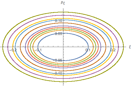
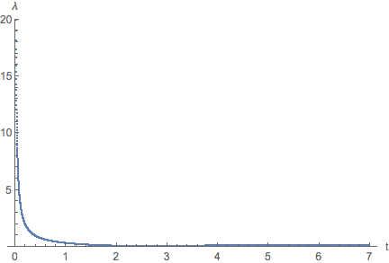
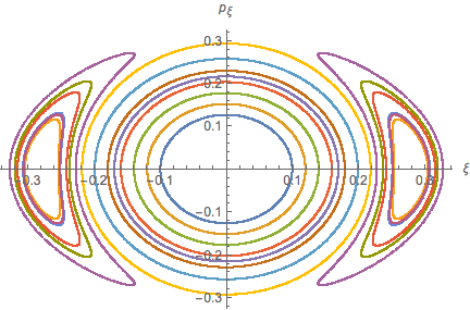
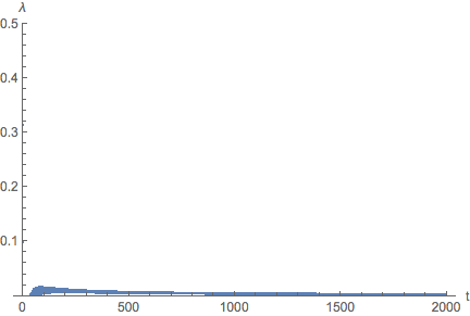
Figure 4: Numerical plots of the Poincaré sections (Left column) and Lyapunov exponents (Right column) for non-relativistic ABJM. Here we set the energy of the string $E_{0}=0.3$. The top plots are for $\mu_{1}=\mu_{2}=\mu_{3}=0.01$ while the bottom plots are for $\mu_{1}=\mu_{2}=\mu_{3}=0.8$. The Poincaré sections are undistorted foliations of KAM tori in the phase space and for large time $t$ the Lyapunov exponent decays to zero. These are indications of the non-chaotic dynamics of the string configuration.

4 Final remarks and future directions

We confirm the non-chaotic dynamics for a class of Yang-Baxter (YB) deformed $\text{AdS}_{4}\times\text{CP}^{3}$ (super) string sigma models. The deformed backgrounds that we considered in our analysis are in fact dual to various deformations of the ABJM model [47] at strong coupling [43]-[46], [60]. These backgrounds are generated through the Yang-Baxter (YB) deformations: there exist classical $r$-matrices that satisfy classical YB equation (1). Interestingly, these deformed backgrounds can be generated by a TsT transformation [60] indicating that they are indeed solutions to the type IIA supergravity.

The primary motivation for our study stemmed from the absence of any systematic analysis of the integrable structures of these class of deformed backgrounds. This is in stark contrast to the undeformed $\text{AdS}_{4}\times\text{CP}^{3}$ case where both analytical and numerical confirmations of the integrability of string sigma models have been established [22]-[24].

In our investigation, we have used both analytical as well as numerical methods. For our analytical computations, we have used the famed Kovacic’s algorithm [4, 5, 6, 17] which checks the Liouvillian (non-)integrability of linear homogeneous second order ordinary differential equations of the form (A1) via a set of necessary but not sufficient criteria. In our analysis, we have been able to recast the dynamical equations of motion of the propagating string in the form of (A1) and checked the fulfilment of the criteria put forward by the algorithm. This established the non-chaotic dynamics of the string in the corresponding deformed backgrounds.

Our analytical results have been substantiated by numerical analysis where we estimated various chaos indicators of the theory namely, the Poincaré section and the Lyapunov exponent. In our computations, using the standard Hamiltonian formulation [1]-[18], we explicitly checked that the shapes of the KAM tori never get distorted as we increase the YB deformation parameters in all the four cases. Also, the Lyapunov exponent decays to zero with time. These two results allow us to conclude that the phase space of the propagating string does not show any chaotic behaviour, thereby establishing consistency with our analytical results. Nevertheless, our analyses do not prove integrability following the traditional Lax pair formulation; rather, it disproves non-integrable structure for certain physical stringy configurations.

The (semi)classical strings, those probe these YB deformed backgrounds, are dual to a class of single trace operators in some sub-sector(s) of these deformed ABJM models. Our analysis, therefore points towards an underlying integrable structure associated with these deformed ABJM models. A systematic analysis of the Lax pairs would further strengthen this claim.

From the perspective of the deformed ABJMs, a similar investigation on the dilatation operators should shed further light on an integrable structure associated with the dual quantum field theory. This would be an interesting future direction to look for which would eventually take us into a new class of Gauge/String dualities those are associated with an underlying integrable structure.

Appendix A The Kovacic’s algorithm

The Kovacic’s algorithm is a systematic method to determine whether a second-order linear homogeneous differential equation of the form

$$\eta^{\prime\prime}(z)+M(z)\eta^{\prime}(z)+N(z)\eta(z)=0\,,$$ (A1)

where $M(z)$, $N(z)$ are polynomial coefficients, are integrable in the Liouvillian sense. This implies the existence of the solutions of (A1) in the form of algebraic functions, trigonometric functions and exponentials.

We here discuss only the necessary details regarding the formalism as the detailed mathematical analysis is rather involved. One wishes to find the relation among $M(z)$, $M^{\prime}(z)$ and $N(z)$ that makes the DE (A1) integrable. In order to achieve this, we start from the change in variable of the form

$$\eta(z)=\exp\quantity[\int\differential z\quantity(w(z)-\frac{M(z)}{2})]\,.$$ (A2)

Eq.(A2) permits us to express (A1) in the following form:

$$w^{\prime}(z)+w^{2}(z)=\mathcal{V}(z)=\frac{2M^{\prime}(z)+M^{2}(z)-4N(z)}{4}\,.$$ (A3)

Now the group of symmetry transformations, $\mathcal{G}$, of the solutions of the DE (A1) is a subgroup of $SL\quantity(2,\mathbb{C})$: $\mathcal{G}\subset SL\quantity(2,\mathbb{C})$. The following four cases are of interest [6, 17]:

1. The subgroup is generated by

   $$\mathcal{G}=\matrixquantity*(a&0\\ b&1/a)\,,\quad a,b\in\mathbb{C}\,.$$

   In this case $w(z)$ is a rational function of degree $1$.

2. The subgroup is generated by

   $$\mathcal{G}=\matrixquantity*(c&0\\ 0&1/c)\,,\quad\mathcal{G}=\matrixquantity*(0&c\\ -1/c&0)\,,\quad c\in\mathbb{C}\,.$$

   In this case $w(z)$ is a rational function of degree $2$.

3. $\mathcal{G}$ is a finite group, excluding the above two possibilities. In this case $w(z)$ is a rational function of degree either $4$, $6$, or $12$.

4. The group $\mathcal{G}$ is $SL(2,\mathbb{C})$. If the solution $w(z)$ at all exists, they non-Liouvillian.

There exists a set of three necessary but not sufficient conditions for the rational polynomial function $\mathcal{V}(z)$ which are compatible with the above group theoretic analysis. These can be enumerated as follows [4, 5]:

1. $\mathcal{V}(z)$ has pole of order $1$, or $2n$ $(n\in\mathbb{Z}^{+})$. Also, the order of $\mathcal{V}(z)$ at infinity is either $2n$ or greater than $2$.

2. $\mathcal{V}(z)$ either has pole of order $2$, or poles of order $2n+1$ greater than $2$.

3. $\mathcal{V}(z)$ has poles not greater than $2$ and the order of $\mathcal{V}(z)$ at infinity is at least $2$.

If any one of these criteria is satisfied, we are eligible to apply the Kovacic’s algorithm to the DE (A1). We then need to determine whether $w(z)$ is a polynomial function of degree $1$, $2$, $4$, $6$, or $12$ in which case (A1) turns out to be integrable. On the contrary, if none of the above criteria is satisfied, the solution to (A1) is non-Liouvillian and ensures the non-integrability of the DE (A1).

Appendix B Numerical Methodology

In the present work, we focus on two chaos indicators namely, the Poincaré section and the Lyapunov exponent [1]-[3]. For the familiarity of the reader, below we briefly elaborate on them and outline basic steps to calculate these entities in a holographic set up.

The signatures of integrability or non-integrability can be differentiated by looking into the phase space dynamics of the system. Integrable systems do not exhibit chaos and the trajectories are (quasi)periodic at equilibrium points. Non-integrable systems, on the other hand, are associated with the phase space that could be mixed showing (quasi)periodic orbits for some initial conditions and chaotic for others.

For a $2N$ dimensional integrable phase space, there are $N$ conserved charges $Q_{i}$, those define an $N$ dimensional hypersurface in the phase space known as the KAM tori. For such systems, the phase space trajectory flows are complete and they appear with a nicely foliated picture of the phase space. Different initial conditions give rise to different sets of trajectories in the phase space those are in the form of the tori. In numerical investigations, Poincaré sections (see left panels of Figs. 1,2, 3,4) are essentially the footprints of such foliations in the phase space [2]. As the strength of the non-integrable deformation increases, most of these tori get destroyed and one essentially runs away from the foliation picture. This results into a chaotic motion and Poincaré sections loose its structure, eventually becoming like a random distribution of points in the phase space.

Lyapunov exponents (see right panels of Figs. 1,2,3, 4), on the other hand, are the signature trademarks of a chaotic motion. They encode the sensitivity of the phase space trajectories on the initial conditions and are defined as[1]-[3]

$$\lambda=\lim_{t\rightarrow\infty}\lim_{\Delta X_{0}\rightarrow 0}\frac{1}{t}\log\frac{\Delta X(X_{0},t)}{\Delta X(X_{0},0)},$$ (B1)

where, $\Delta X$ is the infinitesimal separation between two trajectories in the phase space. For integrable trajectories, those pertaining to a particular KAM tori, the corresponding $\lambda$ approaches zero at late times. On the other hand, it exhibits a nonzero value for chaotic orbits.

To calculate the above entities in a string theory set up, one has to start with the 2D string sigma model description in (2). Given the conjugate momenta (3) and the Hamiltonian (4), we study the corresponding Hamilton’s equations of motion (for a given string embedding) those are subjected to the Virasoro (or the Hamiltonian) constraints of the form [1]

$$\begin{split}\mathcal{H}&=T_{\tau\tau}\approx 0\,,\\ T_{\tau\sigma}&=T_{\sigma\tau}\approx 0\,.\end{split}$$ (B2)

The above constraints (B2) are always satisfied during the time evolution of the system. The initial data that satisfy (B2) are used to find solutions to the Hamilton’s equations of motion corresponding to different backgrounds those are listed above. These solutions are what we call the phase space data those are finally used to explore the chaos indicators mentioned above.

Appendix C Expressions for the coefficients in (13)

$$\begin{split}T^{(1)}_{\theta_{1}}&=-4\alpha_{2}^{2}\quantity(\alpha_{2}^{2}\sin^{2}\theta_{1}\cos^{2}\xi+\cos^{2}\theta_{1}\sin^{2}2\xi\big{/}4)-4\sin^{2}\xi\cos^{2}\xi\Big{(}\alpha_{2}^{2}\cos^{2}\theta_{1}+\alpha_{4}^{2}\cos^{2}\theta_{2}\\ &\quad+4\alpha_{2}\alpha_{6}\cos\theta_{1}-2\alpha_{2}\alpha_{4}\cos\theta_{1}\cos\theta_{2}-4\alpha_{4}\alpha_{6}\cos\theta_{2}\Big{)}-\sin^{2}\theta_{1}\sin^{2}\theta_{2}\sin^{4}2\xi\,\times\\ &\quad\Big{(}\hat{\gamma}_{1}^{2}\alpha_{2}^{2}+2\alpha_{2}\alpha_{4}\hat{\gamma}_{1}\hat{\gamma}_{2}+\hat{\gamma}_{2}^{2}\alpha_{4}^{2}+2\alpha_{2}\alpha_{6}\hat{\gamma}_{1}\hat{\gamma}_{3}+2\alpha_{4}\alpha_{6}\hat{\gamma}_{2}\hat{\gamma}_{3}+\hat{\gamma}_{3}^{2}\alpha_{6}^{2}\Big{)}-4\alpha_{6}^{2}\sin^{2}2\xi\,.\end{split}$$ (C1)

$$\begin{split}T^{(2)}_{\theta_{1}}&=\alpha_{2}^{2}\quantity(4\cos^{2}\xi-\sin^{2}2\xi+\hat{\gamma}_{1}^{2}\sin^{2}\theta_{2}\sin^{4}2\xi)\sin 2\theta_{1}+\quantity(\alpha_{4}\hat{\gamma}_{2}+\alpha_{6}\hat{\gamma}_{3})^{2}\sin 2\theta_{1}\sin^{2}\theta_{2}\times\\ &\quad\sin^{4}2\xi+2\alpha_{2}\Big{[}\alpha_{4}\quantity(\sin\theta_{1}\cos\theta_{2}\sin^{2}2\xi+\hat{\gamma}_{1}\hat{\gamma}_{2}\sin 2\theta_{1}\sin^{2}\theta_{2}\sin^{4}2\xi)+\alpha_{6}\sin^{2}2\xi\,\times\\ &\quad\quantity(-2\sin\theta_{1}+\hat{\gamma}_{1}\hat{\gamma}_{3}\sin 2\theta_{1}\sin^{2}\theta_{2}\sin^{2}2\xi)\Big{]}\,.\end{split}$$ (C2)

$$\begin{split}T^{(1)}_{\theta_{2}}&=-4\alpha_{2}^{2}\cos^{2}\xi\Big{(}\cos^{2}\theta_{1}\sin^{2}\xi+\sin^{2}\theta_{1}\quantity(1+4\hat{\gamma}_{1}^{2}\cos^{2}\xi\sin^{4}\xi\sin^{2}\theta_{2})\Big{)}+8\alpha_{2}\alpha_{4}\\ &\quad\cos^{2}\xi\sin^{2}\xi\quantity(\cos\theta_{1}\cos\theta_{2}-\hat{\gamma}_{1}\hat{\gamma}_{2}\sin^{2}\theta_{1}\sin^{2}\theta_{2}\sin^{2}2\xi)-4\alpha_{4}^{2}\sin^{2}\xi\Big{(}\cos^{2}\theta_{2}\cos^{2}\xi\\ &\quad+\sin^{2}\theta_{2}\quantity(1+4\hat{\gamma}_{2}\sin^{2}\theta_{1}\sin^{2}\xi\cos^{4}\xi)\Big{)}-8\alpha_{2}\alpha_{6}\sin^{2}\xi\cos^{2}\xi\Big{(}2\cos\theta_{1}+\hat{\gamma}_{1}\hat{\gamma}_{3}\sin^{2}\theta_{1}\\ &\quad\sin^{2}\theta_{2}\sin^{2}2\xi\Big{)}+8\alpha_{4}\alpha_{6}\sin^{2}\xi\cos^{2}\xi\quantity(2\cos\theta_{2}-\hat{\gamma}_{2}\hat{\gamma}_{3}\sin^{2}\theta_{1}\sin^{2}\theta_{2}\sin^{2}2\xi)\\ &\quad-\alpha_{6}^{2}\sin^{2}2\xi\quantity(4+\hat{\gamma}_{3}^{2}\sin^{2}\theta_{1}\sin^{2}\theta_{2}\sin^{2}2\xi)\,.\end{split}$$ (C3)

$$\begin{split}T^{(2)}_{\theta_{2}}&=-\quantity(\hat{\gamma}_{1}^{2}\alpha_{2}^{2}+2\hat{\gamma}_{1}\hat{\gamma}_{3}\alpha_{2}\alpha_{6}+\hat{\gamma}_{3}^{2}\alpha_{6}^{2})\,\sin^{2}\theta_{1}\sin 2\theta_{2}\sin^{4}2\xi-2\alpha_{2}\alpha_{4}\sin^{2}2\xi\sin\theta_{2}\\ &\quad\times\quantity(\cos\theta_{1}+2\hat{\gamma}_{1}\hat{\gamma}_{2}\sin^{2}2\xi\sin^{2}\theta_{1}\cos\theta_{2})-4\alpha_{4}^{2}\sin 2\theta_{2}\sin^{4}\xi\quantity(1+4\hat{\gamma}_{2}^{2}\sin^{2}\theta_{1}\cos^{4}\xi)\\ &\quad-2\alpha_{4}\alpha_{6}\sin^{2}2\xi\quantity(2\sin\theta_{2}+\hat{\gamma}_{2}\hat{\gamma}_{3}\sin^{2}\theta_{1}\sin 2\theta_{2}\sin^{2}2\xi)\,.\end{split}$$ (C4)

$$\begin{split}T^{(1)}_{\xi}&=-\quantity(\hat{\gamma}_{1}^{2}\alpha_{2}^{2}+2\hat{\gamma}_{1}\hat{\gamma}_{2}\alpha_{2}\alpha_{4}+\hat{\gamma}_{2}^{2}\alpha_{4}^{2}+\hat{\gamma}_{3}^{2}\alpha_{6}^{2}+2\hat{\gamma}_{1}\hat{\gamma}_{3}\alpha_{2}\alpha_{6}+2\hat{\gamma}_{2}\hat{\gamma}_{3}\alpha_{4}\alpha_{6})\sin^{2}\theta_{1}\sin^{2}\theta_{2}\sin^{4}2\xi\\ &\quad-4\alpha_{2}^{2}\sin^{2}\theta_{1}\cos^{2}\xi-4\alpha_{4}^{2}\sin^{2}\theta_{2}\sin^{2}\xi+\sin^{2}2\xi\Big{(}-4\alpha_{6}^{2}-\alpha_{2}^{2}\cos^{2}\theta_{1}-\alpha_{4}^{2}\cos^{2}\theta_{2}\\ &\quad+2\alpha_{2}\alpha_{4}\cos\theta_{1}\cos\theta_{2}-4\alpha_{2}\alpha_{6}\cos\theta_{1}+4\alpha_{4}\alpha_{6}\cos\theta_{2}\Big{)}\,.\end{split}$$ (C5)

$$\begin{split}T^{(2)}_{\xi}&=-2\Big{(}\alpha_{2}^{2}\quantity(32\hat{\gamma}_{1}^{2}\sin^{3}\xi\cos^{3}\xi\cos 2\xi\sin^{2}\theta_{1}\sin^{2}\theta_{2}-2\sin^{2}\theta_{1}\sin 2\xi+\cos^{2}\theta_{1}\sin 4\xi)\\ &\quad+2\alpha_{2}\sin 4\xi\Big{[}\alpha_{4}\quantity(-\cos\theta_{1}\cos\theta_{2}+2\hat{\gamma}_{1}\hat{\gamma}_{2}\sin^{2}\theta_{1}\sin^{2}\theta_{2}\sin^{2}2\xi)\\ &\quad+2\alpha_{6}\quantity(\cos\theta_{1}+\hat{\gamma}_{1}\hat{\gamma}_{3}\sin^{2}\theta_{1}\sin^{2}\theta_{2}\sin^{2}2\xi)\Big{]}+2\sin 2\xi\Big{[}\alpha_{4}^{2}\Big{(}\cos^{2}\theta_{2}\cos 2\xi+\sin^{2}\theta_{2}\\ &\quad\times\quantity(1+2\hat{\gamma}_{2}^{2}\sin^{2}2\xi\cos 2\xi\sin^{2}\theta_{1})\Big{)}-4\alpha_{4}\alpha_{6}\cos 2\xi\quantity(\cos\theta_{2}-\hat{\gamma}_{2}\hat{\gamma}_{3}\sin^{2}\theta_{1}\sin^{2}\theta_{2}\sin^{2}2\xi)\\ &\quad+2\alpha_{6}^{2}\cos 2\xi\quantity(2+\hat{\gamma}_{3}^{2}\sin^{2}\theta_{1}\sin^{2}\theta_{2}\sin^{2}2\xi)\Big{]}\Big{)}\,.\end{split}$$ (C6)

Appendix D Detailed expressions of $\mathcal{N}_{3}$ and $\mathcal{N}_{4}$ in (109c), (109d)

The expression for $\mathcal{N}_{3}$ in (109c) is given by

$$\mathcal{N}_{3}=-\frac{\mathcal{M}_{1}}{\mathcal{D}_{1}}-\frac{\mathcal{M}_{2}}{64\mathcal{D}_{2}^{2}}+\frac{\mathcal{M}_{3}}{2\mathcal{D}_{1}}-\frac{\mathcal{M}_{4}}{\mathcal{D}_{1}}+\frac{\mathcal{M}_{5}}{\mathcal{D}_{3}^{2}}\,,$$ (D1)

where

$$\mathcal{M}_{1} =\mu_{1}\cos^{4}\xi\sin\theta_{1}\bigg{(}-8\sqrt{2}+2\mu_{2}+4\mu_{3}+2\mu_{1}\cos\theta_{1}+\mu_{1}\cos(\theta_{1}-2\xi)$$

$$+8\sqrt{2}\cos(2\xi)-2\mu_{2}\cos(2\xi)-4\mu_{3}\cos(2\xi)+\mu_{1}\cos(\theta_{1}+2\xi)\bigg{)}$$

$$\times\bigg{(}\mu_{1}^{2}\sin^{2}\theta_{1}+(\mu_{2}+2\mu_{3}-\mu_{1}\cos\theta_{1})^{2}\sin^{2}\xi\bigg{)}\,,$$

$$\mathcal{D}_{1} =16+\cos^{2}\xi\bigg{[}\mu_{1}^{2}\sin^{2}\theta_{1}+\bigg{(}\mu_{2}^{2}-2\mu_{1}(\mu_{2}+2\mu_{3})\cos\theta_{1}+\mu^{2}_{1}\cos^{2}\theta_{1}\bigg{)}\sin^{2}\xi\bigg{]}+\mu_{3}(\mu_{2}$$

$$+\mu_{3})\sin^{2}(2\xi)\,,$$

$$\mathcal{M}_{2} =\mu_{1}\csc^{4}\xi\bigg{(}\big{(}2\big{(}\mu_{2}+2\mu_{3}\big{)}\sin\theta_{1}+\mu_{1}\cot^{2}\xi\sin(2\theta_{1})\big{)}\big{(}256E+4\mu_{1}^{2}\cos^{2}\xi\sin^{2}\theta_{1}$$

$$+\big{(}\mu_{2}+2\mu_{3}-\mu_{1}\cos\theta_{1}\big{)}\big{(}-8\sqrt{2}+\mu_{2}+2\mu_{3}-\mu_{1}\cos\theta_{1}\big{)}\sin^{2}(2\xi)\big{)}^{2}\bigg{)}\,,$$

$$\mathcal{D}_{2}=\big{(}\mu_{2}+2\mu_{3}-\mu_{1}\cos\theta_{1}\big{)}^{2}\cos^{2}\xi+16\csc^{2}\xi+\mu_{1}^{2}\cot^{2}\xi\sin^{2}\theta_{1}\,,$$

$$\mathcal{M}_{3} =\mu_{1}\cos^{2}\xi\bigg{(}-8\sqrt{2}+2\mu_{2}+4\mu_{3}+2\mu_{1}\cos\theta_{1}+\mu_{1}\cos(\theta_{1}-2\xi)+8\sqrt{2}\cos(2\xi)$$

$$-2\mu_{2}\cos(2\xi)-4\mu_{3}\cos(2\xi)+\mu_{1}\cos(\theta_{1}+2\xi)\bigg{)}\sin\theta_{1}\bigg{(}128E$$

$$+2\mu_{1}^{2}\cos^{2}\xi\big{(}\sin^{2}\theta_{1}+\cos^{2}\theta_{1}\sin^{2}\xi\big{)}-\frac{1}{2}\big{(}\big{(}8\sqrt{2}-\mu_{2}-2\mu_{3}\big{)}(\mu_{2}+2\mu_{3})$$

$$+2\mu_{1}\big{(}-4\sqrt{2}+\mu_{2}+2\mu_{3}\big{)}\cos\theta_{1}\big{)}\sin^{2}(2\xi)\bigg{)}\,,$$

$$\mathcal{M}_{4}= \mu_{1}\cos^{2}\xi\bigg{(}\mu_{1}\cos^{2}\xi\sin(2\theta_{1})+2(\mu_{2}+2\mu_{3})\sin\theta_{1}\sin^{2}\xi\bigg{)}\times\bigg{(}128E$$

$$+2\mu_{1}^{2}\cos^{2}\xi\big{(}\sin^{2}\theta_{1}+\cos^{2}\theta_{1}\sin^{2}\xi\big{)}-\frac{1}{2}\big{(}\big{(}8\sqrt{2}-\mu_{2}-2\mu_{3}\big{)}(\mu_{2}+2\mu_{3})$$

$$+2\mu_{1}\big{(}-4\sqrt{2}+\mu_{2}+2\mu_{3}\big{)}\cos\theta_{1}\big{)}\sin^{2}(2\xi)\bigg{)}\,,$$

$$\mathcal{M}_{5} =\mu_{1}\cos^{4}\xi\big{(}\mu_{2}+2\mu_{3}+\mu_{1}\cos\theta_{1}\cot^{2}\xi\big{)}\bigg{(}\mu_{1}^{2}\cot^{2}\xi-2\mu_{1}(\mu_{2}+2\mu_{3})\cot\theta_{1}\csc\theta_{1}$$

$$+\big{(}\mu_{2}+2\mu_{3}\big{)}^{2}\csc^{2}\theta_{1}+\mu_{1}^{2}\csc^{2}\xi\bigg{)}\sin\theta_{1}\bigg{(}4\mu_{1}^{2}\cos^{2}\xi+\mu_{1}^{2}\cot^{2}\theta_{1}\sin^{2}(2\xi)$$

$$+2\mu_{1}\big{(}4\sqrt{2}-\mu_{2}-2\mu_{3}\big{)}\cot\theta_{1}\csc\theta_{1}\sin^{2}(2\xi)+\csc^{2}\theta_{1}\big{(}256E$$

$$-\big{(}8\sqrt{2}-\mu_{2}-2\mu_{3}\big{)}(\mu_{2}+2\mu_{3})\sin^{2}(2\xi)\big{)}\bigg{)}\,,$$

$$\mathcal{D}_{3}=\mu_{1}^{2}\cot^{2}\xi+\big{(}\mu_{2}+2\mu_{3}-\mu_{1}\cos\theta_{1}\big{)}^{2}\cos^{2}\xi\csc^{2}\theta_{1}+16\csc^{2}\theta_{1}\csc^{2}\xi\,.$$

The expression for $\mathcal{N}_{4}$ in (109d) is given by

$$\mathcal{N}_{4}=\frac{\mathcal{M}_{6}}{2\mathcal{D}_{2}}+\frac{\mathcal{M}_{7}}{\mathcal{D}_{1}}+\frac{\mathcal{M}_{8}}{\mathcal{D}_{1}^{2}}-\frac{\mathcal{M}_{9}}{\mathcal{D}_{1}^{2}}-\frac{\mathcal{M}_{10}}{\mathcal{D}_{1}}+\frac{2\mathcal{M}_{11}}{\mathcal{D}_{1}}\,,$$ (D2)

where

$$\mathcal{M}_{6} =16\sin^{2}\theta_{1}\sin(2\xi)\big{(}\mu_{2}+2\mu_{3}-\mu_{1}\cos\theta_{1}\big{)}^{2}\csc^{2}\xi\bigg{(}\big{(}\mu_{2}+2\mu_{3}-\mu_{1}\cos\theta_{1}\big{)}\big{(}-8\sqrt{2}+\mu_{2}$$

$$+2\mu_{3}-\mu_{1}\cos\theta_{1}\big{)}\cos^{2}\xi+64E\csc^{2}\xi+\mu_{1}^{2}\cot^{2}\xi\sin^{2}\theta_{1}\bigg{)}\sin^{3}(2\xi)\,,$$

$$\mathcal{M}_{7} =\bigg{(}\mu_{1}^{2}\sin^{2}\theta_{1}+\big{(}\mu_{2}+2\mu_{3}-\mu_{1}\cos\theta_{1}\big{)}^{2}\sin^{2}\xi\bigg{)}\sin(2\xi)\bigg{(}128E$$

$$+2\mu_{1}^{2}\cos^{2}\xi\big{(}\sin^{2}\theta_{1}+\cos^{2}\theta_{1}\sin^{2}\xi\big{)}-\frac{1}{2}\big{(}\big{(}8\sqrt{2}-\mu_{2}-2\mu_{3}\big{)}(\mu_{2}+2\mu_{3})$$

$$+2\mu_{1}\big{(}-4\sqrt{2}+\mu_{2}+2\mu_{3}\big{)}\cos\theta_{1}\big{)}\sin^{2}(2\xi)\bigg{)}\,,$$

$$\mathcal{M}_{8} =2\mu_{3}^{2}\sin(4\xi)+\bigg{(}2\cos^{2}\xi\big{(}\mu_{1}^{2}\sin^{2}\theta_{1}+\big{(}\mu_{2}+2\mu_{3}-\mu_{1}\cos\theta_{1}\big{)}^{2}\sin^{2}(\xi)\big{)}\bigg{)}$$

$$\times\bigg{(}64E+\cos^{2}\xi\big{(}\mu_{1}^{2}\sin^{2}\theta_{1}+\big{(}\mu_{2}-\mu_{1}\cos\theta_{1}\big{)}\big{(}\mu_{2}+4\mu_{3}-\mu_{1}\cos\theta_{1}\big{)}\sin^{2}\xi\big{)}+\mu_{3}^{2}\sin^{2}(2\xi)$$

$$-2\sqrt{2}\big{(}\mu_{2}+2\mu_{3}-\mu_{1}\cos\theta_{1}\big{)}\sin^{2}(2\xi)\bigg{)}\bigg{(}2\big{(}\mu_{2}-\mu_{1}\cos\theta_{1}\big{)}\big{(}\mu_{2}+4\mu_{3}-\mu_{1}\cos\theta_{1}\big{)}\cos^{3}\xi\sin\xi$$

$$-2\cos\xi\sin\xi\big{(}\mu_{1}^{2}\sin^{2}\theta_{1}+\big{(}\mu_{2}-\mu_{1}\cos\theta_{1}\big{)}\times\big{(}\mu_{2}+4\mu_{3}-\mu_{1}\cos\theta_{1}\big{)}\sin^{2}\xi\big{)}+2\mu_{3}^{2}\sin(4\xi)\bigg{)}\,,$$

$$\mathcal{M}_{9} =\bigg{(}64E+\cos^{2}\xi\big{(}\mu_{1}^{2}\sin^{2}\theta_{1}+\big{(}\mu_{2}-\mu_{1}\cos\theta_{1}\big{)}\big{(}\mu_{2}+4\mu_{3}-\mu_{1}\cos\theta_{1}\big{)}\sin^{2}\xi\big{)}+\mu_{3}^{2}\sin^{2}(2\xi)$$

$$-2\sqrt{2}\big{(}\mu_{2}+2\mu_{3}-\mu_{1}\cos\theta_{1}\big{)}\sin^{2}(2\xi)\bigg{)}^{2}\bigg{(}2\big{(}\mu_{2}-\mu_{1}\cos\theta_{1}\big{)}\big{(}\mu_{2}+4\mu_{3}-\mu_{1}\cos\theta_{1}\big{)}\cos^{3}\xi\sin\xi$$

$$-2\cos\xi\sin\xi\big{(}\mu_{1}^{2}\sin^{2}\theta_{1}+\big{(}\mu_{2}-\mu_{1}\cos\theta_{1}\big{)}\times\big{(}\mu_{2}+4\mu_{3}-\mu_{1}\cos\theta_{1}\big{)}\sin^{2}\xi\big{)}+2\mu_{3}^{2}\sin(4\xi)\bigg{)}\,,$$

$$\mathcal{M}_{10} =\bigg{(}2\cos^{2}\xi\big{(}\mu_{1}^{2}\sin^{2}\theta_{1}+\big{(}\mu_{2}+2\mu_{3}-\mu_{1}\cos\theta_{1}\big{)}^{2}\sin^{2}\xi\big{)}\bigg{)}$$

$$\bigg{(}2\big{(}\mu_{2}-\mu_{1}\cos\theta_{1}\big{)}\big{(}\mu_{2}+4\mu_{3}-\mu_{1}\cos\theta_{1}\big{)}\cos^{3}\xi\sin\xi$$

$$-2\cos\xi\sin\xi\big{(}\mu_{1}^{2}\sin^{2}\theta_{1}+\big{(}\mu_{2}-\mu_{1}\cos\theta_{1}\big{)}\times\big{(}\mu_{2}+4\mu_{3}-\mu_{1}\cos\theta_{1}\big{)}\sin^{2}\xi\big{)}$$

$$+2\mu_{3}^{2}\sin(4\xi)-4\sqrt{2}\big{(}\mu_{2}+2\mu_{3}-\mu_{1}\cos\theta_{1}\big{)}\sin(4\xi)\bigg{)}\,,$$

$$\mathcal{M}_{11} =\bigg{(}64E+\cos^{2}\xi\big{(}\mu_{1}^{2}\sin^{2}\theta_{1}+\big{(}\mu_{2}-\mu_{1}\cos\theta_{1}\big{)}\big{(}\mu_{2}+4\mu_{3}-\mu_{1}\cos\theta_{1}\big{)}\sin^{2}\xi\big{)}+\mu_{3}^{2}\sin^{2}(2\xi)$$

$$-2\sqrt{2}\big{(}\mu_{2}+2\mu_{3}-\mu_{1}\cos\theta_{1}\big{)}\sin^{2}(2\xi)\bigg{)}\bigg{(}2\big{(}\mu_{2}-\mu_{1}\cos\theta_{1}\big{)}\big{(}\mu_{2}+4\mu_{3}-\mu_{1}\cos\theta_{1}\big{)}\cos^{3}\xi\sin\xi$$

$$-2\cos\xi\sin\xi\big{(}\mu_{1}^{2}\sin^{2}\theta_{1}+\big{(}\mu_{2}-\mu_{1}\cos\theta_{1}\big{)}\times\big{(}\mu_{2}+4\mu_{3}-\mu_{1}\cos\theta_{1}\big{)}\sin^{2}\xi\big{)}+2\mu_{3}^{2}\sin(4\xi)$$

$$-4\sqrt{2}\big{(}\mu_{2}+2\mu_{3}-\mu_{1}\cos\theta_{1}\big{)}\sin(4\xi)\bigg{)}\,.$$

References

- [1] L. A. Pando Zayas and C. A. Terrero-Escalante, “Chaos in the Gauge / Gravity Correspondence,” JHEP 1009, 094 (2010) doi:10.1007/JHEP09(2010)094 [arXiv:1007.0277 [hep-th]].
- [2] P. Basu, D. Das and A. Ghosh, “Integrability Lost,” Phys. Lett. B 699, 388 (2011) doi:10.1016/j.physletb.2011.04.027 [arXiv:1103.4101 [hep-th]].
- [3] P. Basu and L. A. Pando Zayas, “Chaos rules out integrability of strings on ” Phys. Lett. B 700, 243 (2011) doi:10.1016/j.physletb.2011.04.063 [arXiv:1103.4107 [hep-th]].
- [4] J. J. Kovacic, “An algorithm for solving second order linear homogeneous differential equations,” J.Symb.Comput. 2 (1986) 3 .
- [5] B. D. Saunders, “An implementation of Kovacic’s algorithm for solving second order linear homogeneous differential equations,” in: The Proceedings of the 4th ACM Symposium on Symbolic and Algebraic Computation, SYMSAC’81, August 5–7, Snowbird, USA, 1981.
- [6] J. Kovacic, “Picard-Vessiot Theory, Algebraic Groups and Group Schemes,” Department of Mathematics, the City College of the City University of New York, 2005, https://ksda.ccny.cuny.edu/PostedPapers/pv093005.pdf
- [7] P. Basu and L. A. Pando Zayas, “Analytic Non-integrability in String Theory,” Phys. Rev. D 84 (2011), 046006 doi:10.1103/PhysRevD.84.046006 [arXiv:1105.2540 [hep-th]].
- [8] P. Basu, D. Das, A. Ghosh and L. A. Pando Zayas, “Chaos around Holographic Regge Trajectories,” JHEP 1205, 077 (2012) doi:10.1007/JHEP05(2012)077 [arXiv:1201.5634 [hep-th]].
- [9] L. A. Pando Zayas and D. Reichmann, “A String Theory Explanation for Quantum Chaos in the Hadronic Spectrum,” JHEP 1304, 083 (2013) doi:10.1007/JHEP04(2013)083 [arXiv:1209.5902 [hep-th]].
- [10] P. Basu and A. Ghosh, “Confining Backgrounds and Quantum Chaos in Holography,” Phys. Lett. B 729, 50 (2014) doi:10.1016/j.physletb.2013.12.052 [arXiv:1304.6348[hep-th]].
- [11] P. Basu, P. Chaturvedi and P. Samantray, “Chaotic dynamics of strings in charged black hole backgrounds,” Phys. Rev. D 95, no.6, 066014 (2017) doi:10.1103/PhysRevD.95.066014 [arXiv:1607.04466 [hep-th]].
- [12] K. L. Panigrahi and M. Samal, “Chaos in classical string dynamics in deformed ,” Phys. Lett. B 761, 475-481 (2016) doi:10.1016/j.physletb.2016.08.021 [arXiv:1605.05638 [hep-th]].
- [13] D. Giataganas, L. A. Pando Zayas and K. Zoubos, “On Marginal Deformations and Non-Integrability,” JHEP 1401, 129 (2014) doi:10.1007/JHEP01(2014)129 [arXiv:1311.3241 [hep-th]].
- [14] T. Ishii, S. Kushiro and K. Yoshida, “Chaotic string dynamics in deformed T1,1,” JHEP 05, 158 (2021) doi:10.1007/JHEP05(2021)158 [arXiv:2103.12416 [hep-th]].
- [15] D. Roychowdhury, “Analytic integrability for strings on and deformed backgrounds,” JHEP 10 (2017), 056 doi:10.1007/JHEP10(2017)056 [arXiv:1707.07172 [hep-th]].
- [16] C. Núñez, J. M. Penín, D. Roychowdhury and J. Van Gorsel, “The non-Integrability of Strings in Massive Type IIA and their Holographic duals,” JHEP 06 (2018), 078 doi:10.1007/JHEP06(2018)078 [arXiv:1802.04269 [hep-th]].
- [17] C. Núñez, D. Roychowdhury and D. C. Thompson, “Integrability and non-integrability in SCFTs and their holographic backgrounds,” JHEP 07 (2018), 044 doi:10.1007/JHEP07(2018)044 [arXiv:1804.08621 [hep-th]].
- [18] A. Banerjee and A. Bhattacharyya, “Probing analytical and numerical integrability: the curious case of (AdS)η,” JHEP 11 (2018), 124 doi:10.1007/JHEP11(2018)124 [arXiv:1806.10924 [hep-th]].
- [19] J. M. Maldacena, “The Large N limit of superconformal field theories and supergravity,” Adv. Theor. Math. Phys. 2 (1998), 231-252 doi:10.1023/A:1026654312961 [arXiv:hep-th/9711200 [hep-th]].
- [20] E. Witten, “Anti-de Sitter space and holography,” Adv. Theor. Math. Phys. 2 (1998), 253-291 doi:10.4310/ATMP.1998.v2.n2.a2 [arXiv:hep-th/9802150 [hep-th]].
- [21] I. Bena, J. Polchinski and R. Roiban, “Hidden symmetries of the superstring,” Phys. Rev. D 69 (2004), 046002 doi:10.1103/PhysRevD.69.046002 [arXiv:hep-th/0305116 [hep-th]].
- [22] G. Arutyunov and S. Frolov, “Superstrings on as a Coset Sigma-model,” JHEP 09, 129 (2008) doi:10.1088/1126-6708/2008/09/129 [arXiv:0806.4940 [hep-th]].
- [23] B. Stefanski, jr, “Green-Schwarz action for Type IIA strings on ,” Nucl. Phys. B 808, 80-87 (2009) doi:10.1016/j.nuclphysb.2008.09.015 [arXiv:0806.4948 [hep-th]].
- [24] D. Sorokin and L. Wulff, “Evidence for the classical integrability of the complete superstring,” JHEP 11 (2010), 143 doi:10.1007/JHEP11(2010)143 [arXiv:1009.3498 [hep-th]].
- [25] K. Zarembo, “Strings on Semisymmetric Superspaces,” JHEP 05 (2010), 002 doi:10.1007/JHEP05(2010)002 [arXiv:1003.0465 [hep-th]].
- [26] O. Lunin and J. M. Maldacena, “Deforming field theories with U(1) x U(1) global symmetry and their gravity duals,” JHEP 05, 033 (2005) doi:10.1088/1126-6708/2005/05/033 [arXiv:hep-th/0502086 [hep-th]].
- [27] S. A. Frolov, R. Roiban and A. A. Tseytlin, “Gauge-string duality for superconformal deformations of N=4 super Yang-Mills theory,” JHEP 07 (2005), 045 doi:10.1088/1126-6708/2005/07/045 [arXiv:hep-th/0503192 [hep-th]].
- [28] S. Frolov, “Lax pair for strings in Lunin-Maldacena background,” JHEP 05 (2005), 069 doi:10.1088/1126-6708/2005/05/069 [arXiv:hep-th/0503201 [hep-th]].
- [29] D. Giataganas, L. A. Pando Zayas and K. Zoubos, “On Marginal Deformations and Non-Integrability,” JHEP 01 (2014), 129 doi:10.1007/JHEP01(2014)129 [arXiv:1311.3241 [hep-th]].
- [30] C. Klimcik, “Yang-Baxter sigma models and dS/AdS T duality,” JHEP 12, 051 (2002) doi:10.1088/1126-6708/2002/12/051 [arXiv:hep-th/0210095 [hep-th]].
- [31] C. Klimcik, “On integrability of the Yang-Baxter sigma-model,” J. Math. Phys. 50, 043508 (2009) doi:10.1063/1.3116242 [arXiv:0802.3518 [hep-th]].
- [32] F. Delduc, M. Magro and B. Vicedo, “On classical -deformations of integrable sigma-models,” JHEP 11, 192 (2013) doi:10.1007/JHEP11(2013)192 [arXiv:1308.3581 [hep-th]].
- [33] F. Delduc, M. Magro and B. Vicedo, “An integrable deformation of the superstring action,” Phys. Rev. Lett. 112, no.5, 051601 (2014) doi:10.1103/PhysRevLett.112.051601 [arXiv:1309.5850 [hep-th]].
- [34] F. Delduc, M. Magro and B. Vicedo, “Derivation of the action and symmetries of the -deformed superstring,” JHEP 10, 132 (2014) doi:10.1007/JHEP10(2014)132 [arXiv:1406.6286 [hep-th]].
- [35] G. Arutyunov, R. Borsato and S. Frolov, “S-matrix for strings on -deformed AdS5 x S5,” JHEP 04, 002 (2014) doi:10.1007/JHEP04(2014)002 [arXiv:1312.3542 [hep-th]].
- [36] G. Arutyunov, R. Borsato and S. Frolov, “Puzzles of -deformed AdS S5,” JHEP 12, 049 (2015) doi:10.1007/JHEP12(2015)049 [arXiv:1507.04239 [hep-th]].
- [37] G. Arutyunov, S. Frolov, B. Hoare, R. Roiban and A. A. Tseytlin, “Scale invariance of the -deformed superstring, T-duality and modified type II equations,” Nucl. Phys. B 903, 262-303 (2016) doi:10.1016/j.nuclphysb.2015.12.012 [arXiv:1511.05795 [hep-th]].
- [38] B. Hoare and F. K. Seibold, “Supergravity backgrounds of the -deformed AdS and AdS superstrings,” JHEP 01, 125 (2019) doi:10.1007/JHEP01(2019)125 [arXiv:1811.07841 [hep-th]].
- [39] I. Kawaguchi, T. Matsumoto and K. Yoshida, “Jordanian deformations of the superstring,” JHEP 04, 153 (2014) doi:10.1007/JHEP04(2014)153 [arXiv:1401.4855 [hep-th]].
- [40] T. Matsumoto and K. Yoshida, “Lunin-Maldacena backgrounds from the classical Yang-Baxter equation - towards the gravity/CYBE correspondence,” JHEP 06, 135 (2014) doi:10.1007/JHEP06(2014)135 [arXiv:1404.1838 [hep-th]].
- [41] G. Linardopoulos, “String integrability of the ABJM defect,” JHEP 06, 033 (2022) doi:10.1007/JHEP06(2022)033 [arXiv:2202.06824 [hep-th]].
- [42] T. Matsumoto and K. Yoshida, “Schrödinger geometries arising from Yang-Baxter deformations,” JHEP 04, 180 (2015) doi:10.1007/JHEP04(2015)180 [arXiv:1502.00740 [hep-th]].
- [43] R. Negrón and V. O. Rivelles, “Yang-Baxter deformations of the superstring sigma model,” JHEP 11, 043 (2018) doi:10.1007/JHEP11(2018)043 [arXiv:1809.01174 [hep-th]].
- [44] L. Rado, V. O. Rivelles and R. Sánchez, “String backgrounds of the Yang-Baxter deformed superstring,” JHEP 01, 056 (2021) doi:10.1007/JHEP01(2021)056 [arXiv:2009.04397 [hep-th]].
- [45] L. Rado, V. O. Rivelles and R. Sánchez, “Bosonic -deformations of non-integrable backgrounds,” JHEP 03, 094 (2022) doi:10.1007/JHEP03(2022)094 [arXiv:2111.13169 [hep-th]].
- [46] L. Rado, V. O. Rivelles and R. Sánchez, “Bosonic -deformed Background,” JHEP 10, 115 (2021) doi:10.1007/JHEP10(2021)115 [arXiv:2105.07545 [hep-th]].
- [47] O. Aharony, O. Bergman, D. L. Jafferis and J. Maldacena, “N=6 superconformal Chern-Simons-matter theories, M2-branes and their gravity duals,” JHEP 10, 091 (2008) doi:10.1088/1126-6708/2008/10/091 [arXiv:0806.1218 [hep-th]].
- [48] S. J. van Tongeren, “On classical Yang-Baxter based deformations of the superstring,” JHEP 06, 048 (2015) doi:10.1007/JHEP06(2015)048 [arXiv:1504.05516 [hep-th]].
- [49] D. Osten and S. J. van Tongeren, “Abelian Yang–Baxter deformations and TsT transformations,” Nucl. Phys. B 915, 184-205 (2017) doi:10.1016/j.nuclphysb.2016.12.007 [arXiv:1608.08504 [hep-th]].
- [50] I. Bakhmatov, Ö. Kelekci, E. Ó Colgáin and M. M. Sheikh-Jabbari, “Classical Yang-Baxter Equation from Supergravity,” Phys. Rev. D 98, no.2, 021901 (2018) doi:10.1103/PhysRevD.98.021901 [arXiv:1710.06784 [hep-th]].
- [51] I. Bakhmatov, E. Ó Colgáin, M. M. Sheikh-Jabbari and H. Yavartanoo, “Yang-Baxter Deformations Beyond Coset Spaces (a slick way to do TsT),” JHEP 06, 161 (2018) doi:10.1007/JHEP06(2018)161 [arXiv:1803.07498 [hep-th]].
- [52] B. Hoare and A. A. Tseytlin, “Homogeneous Yang-Baxter deformations as non-abelian duals of the -model,” J. Phys. A 49, no.49, 494001 (2016) doi:10.1088/1751-8113/49/49/494001 [arXiv:1609.02550 [hep-th]].
- [53] D. Orlando, S. Reffert, J. i. Sakamoto and K. Yoshida, “Generalized type IIB supergravity equations and non-Abelian classical r-matrices,” J. Phys. A 49, no.44, 445403 (2016) doi:10.1088/1751-8113/49/44/445403 [arXiv:1607.00795 [hep-th]].
- [54] R. Borsato and L. Wulff, “Target space supergeometry of and -deformed strings,” JHEP 10, 045 (2016) doi:10.1007/JHEP10(2016)045 [arXiv:1608.03570 [hep-th]].
- [55] S. J. van Tongeren, “Almost abelian twists and AdS/CFT,” Phys. Lett. B 765, 344-351 (2017) doi:10.1016/j.physletb.2016.12.002 [arXiv:1610.05677 [hep-th]].
- [56] T. Matsumoto and K. Yoshida, “Yang–Baxter sigma models based on the CYBE,” Nucl. Phys. B 893 (2015), 287-304 doi:10.1016/j.nuclphysb.2015.02.009 [arXiv:1501.03665 [hep-th]].
- [57] B. Hoare and S. J. van Tongeren, “On jordanian deformations of AdS5 and supergravity,” J. Phys. A 49, no.43, 434006 (2016) doi:10.1088/1751-8113/49/43/434006 [arXiv:1605.03554 [hep-th]].
- [58] T. Matsumoto and K. Yoshida, “Integrability of classical strings dual for noncommutative gauge theories,” JHEP 06, 163 (2014) doi:10.1007/JHEP06(2014)163 [arXiv:1404.3657 [hep-th]].
- [59] T. Matsumoto and K. Yoshida, “Integrable deformations of the AdS superstring and the classical Yang-Baxter equation ,” J. Phys. Conf. Ser. 563, no.1, 012020 (2014) doi:10.1088/1742-6596/563/1/012020 [arXiv:1410.0575 [hep-th]].
- [60] E. Imeroni, “On deformed gauge theories and their string/M-theory duals,” JHEP 10, 026 (2008) doi:10.1088/1126-6708/2008/10/026 [arXiv:0808.1271 [hep-th]].
- [61] J. Polchinski, “String theory. Vol. 1: An introduction to the bosonic string,” Cambridge University Press, 2007, ISBN 978-0-511-25227-3, 978-0-521-67227-6, 978-0-521-63303-1 doi:10.1017/CBO9780511816079