Study of Novel Sparse Array Design Based on the Maximum Inter-Element Spacing Criterion

Abstract

A novel sparse array (SA) structure is proposed based on the maximum inter-element spacing (IES) constraint (MISC) criterion. Compared with the traditional MISC array, the proposed SA configurations, termed as improved MISC (IMISC) has significantly increased uniform degrees of freedom (uDOF) and reduced mutual coupling. In particular, the IMISC arrays are composed of six uniform linear arrays (ULAs), which can be determined by an IES set. The IES set is constrained by two parameters, namely the maximum IES and the number of sensors. The uDOF of the IMISC arrays is derived and the weight function of the IMISC arrays is analyzed as well. The proposed IMISC arrays have a great advantage in terms of uDOF against the existing SAs, while their mutual coupling remains at a low level. Simulations are carried out to demonstrate the advantages of the IMISC arrays.

I Introduction

There is a growing body of literature that emphasizes the vital role of sensor array techniques in diverse applications, such as seismology [1], radar [2], sonar [3], and others. An important problem in sensor array technique is direction finding [4], especially the case when there are more targets than the number of sensors [1, 5]. In this context, the difference coarray (DCA) principle is one of the feasible choices to produce plenty uniform degrees of freedom (uDOF), which makes possible to use fewer sensors estimate more targets [8, 6, 7]. Based on the DCA concept, many classical sparse arrays (SAs) have been introduced, among which the nested arrays (NAs) [9] and coprime arrays (CAs) are very popular [10, 11, 12, 13, 14]. The NAs can achieve $O(N^{2}/2)$ uDOF using $N$ sensors but are sensitive to the mutual coupling (MC) among sensors. Unlike NAs, CAs are robust to MC, but their uDOF are less than those of NAs [10, 11].

Many existing SAs have been developed via the prototype NAs and CAs  [15, 16, 18, 17, 12]. Early SAs have focused on increasing the achievable uDOF. To this end, the improved NA (INA) [15], the CA with displaced subarrays (CADiS) [16] and the two side-extended nested array (TSENA) [17] are proposed. These SAs show considerable improvement on uDOF. However, with the growing of electromagnetic equipments, MC is inevitable and needs to be considered when designing SAs. In this regard, several SAs have been proposed based on NAs and CAs. For example, the super nested arrays (SNAs) [19, 20, 21, 22], the extended padded coprime arrays (ePCAs) [23] and the improved coprime nested arrays (ICNA) [24] are examples of SAs designed based on NAs and CAs. It is worth noting that the ICNA realizes $O(4Q^{2}/7)$ uDOFs with $Q$ sensor elements and MC among sensors is very low. Another general SA design method is the ULA fitting scheme, based on which the ULA fitting with 4 base layer (UF-4BL) has been proposed with low MC [26, 25]. Beyond the aforementioned SA design approaches, the maximum inter-element spacing (IES) constraint (MISC) criterion is also promising [27]. The MISC criterion aims to design SAs with an inter-element spacing set, which is constrained by the maximum element spacing and the number of sensors. The MISC arrays provide a good balance between MC and uDOF.

In this work, we develop an improved MISC (IMISC) array based on the MISC approach with an increased uDOF and reduced MC as compared to the traditional MISC array. In particular, we carry out an analysis that shows that IMISC arrays reach $O(2Q^{2}/3)$ uDOF, which is significantly higher than those uDOF achieved by existing sparse arrays. Moreover, the MC of the proposed IMISC arrays remains at a reduced level. Simulations illustrate the excellent performance of the proposed IMISC arrays.

II Coarray Concept and Mutual Coupling

II-A Difference Coarray Model

Let us assume an $Q$-sensor linear array with location set

$$\mathbb{L}=\left\{{{p_{0}},p_{1},p_{2},\dots,p_{Q-1}}\right\},$$ (1)

then the associated steering vector can be obtained as $\mathbf{v}_{\phi}=\left[e^{j\frac{2\pi}{\lambda}p_{0}/\sin(\phi)},\cdots,e^{j\frac{2\pi}{\lambda}p_{Q-1}/\sin(\phi)}\right]^{T}$, where $\phi$ is the signal impinging direction. Then imagine $R$ uncorrelated far-field narrowband signals impinging from directions $\left\{\phi_{i},i=1,\cdots,R\right\}$ with powers $\left\{\sigma^{2}_{i},i=1,\cdots,R\right\}$. In this regard, the observed signal can be expressed as

$${\mathbf{x}}={\mathbf{V}}{\mathbf{s}}+{\mathbf{n}},$$ (2)

where $\mathbf{V}\triangleq\left[\mathbf{v}_{\phi_{1}},\cdots,\mathbf{v}_{\phi_{R}}\right]$ is the array manifold matrix, $\mathbf{s}\triangleq\left[\mathbf{s}_{1},\cdots,\mathbf{s}_{R}\right]^{T}$ denotes the signal vector, ${\mathbf{n}}$ is the white Gaussian noise with zero mean. Then, the covariance matrix of (2) can be calculated as

$${\mathbf{R}_{\mathbf{x}}}\triangleq E[\mathbf{x}{\mathbf{x}^{H}}]=\mathbf{V}\mathbf{R}_{\mathbf{s}}{\mathbf{V}^{H}}+\sigma_{n}^{2}\mathbf{I},$$ (3)

where $\sigma^{2}_{n}$ is the power of noise and $\mathbf{R}_{\mathbf{s}}$ represents the signal covariance matrix. In this case, the vectorized version of (3) can be obtained as

$${\mathbf{w}}\triangleq{\rm{vec}}({\mathbf{R}_{\mathbf{x}}})=({\mathbf{V}}^{*}\odot{\mathbf{V}}){\mathbf{q}}+\sigma_{n}^{2}{\mathbf{1}}_{n},$$ (4)

where ${\mathbf{1}}_{n}={\rm{vec}}({\mathbf{I}}_{N})$, ${\mathbf{q}}=\left[\sigma^{2}_{1},\cdots,\sigma^{2}_{R}\right]^{T}$, and $\odot$ means the Khatri-Rao product. The DCA concept originates from (4), where ${\mathbf{q}}$ serves as the observed signal of the DCA. Based on (4), the DCA of array $\mathbb{L}$ has the following position set [9]

$$\mathbb{D}=\left\{{{p_{a}-p_{b}},a,b=0,1,\cdots Q-1}\right\}.$$ (5)

II-B Coupling Leakage

In practice, the MC among sensors should be considered. To this end, the MC matrix $\mathbf{A}$ can be interpolated into (2), resulting in

$${\mathbf{x}}={\mathbf{A}}{\mathbf{V}}{\mathbf{s}}+{\mathbf{n}},$$ (6)

Based on [27, 28, 29], the MC matrix for linear arrays can be formulated as a $D$-banded matrix given by

$${\mathbf{A}}_{b,c}=\left\{{\begin{array}[]{*{20}{l}}a_{|p_{b}-p_{c}|},&|p_{b}-p_{c}|\leq D,\\ 0,&{\rm{elsewhere}},\end{array}}\right.$$ (7)

where $p_{b},p_{c}\in\mathbb{L}$ and $a_{d},d\in[0,D]$ represent elements in $\mathbf{A}$ that satisfy

$$\left\{{\begin{array}[]{*{20}{l}}a_{0}=1\textgreater|a_{1}|\textgreater|a_{2}|\textgreater\cdots\textgreater|a_{D}|,\\ |a_{i}/a_{j}|=j/i,\quad i,j\in[{\color[rgb]{1,0,0}1},D].\end{array}}\right.$$ (8)

Coupling leakage is a parameter to evaluate the MC effect, which is expressed as [21, 18, 27]

$$E=\frac{||{\mathbf{A}}-{\rm{diag}}({\mathbf{A}})||_{F}}{||{\mathbf{A}}||_{F}}.$$ (9)

Typically, higher coupling leakage means larger MC. Moreover, equations (7), (8) and (9) reveal the relationship between MC and the weight function $w(n)$. For linear arrays, the weight function $w(n)$ indicates the number of element pairs whose IES is $n$. For SA $\mathbb{L}$, $w(n)$ can be obtained as [27]

$$w(n)=|\{(p_{i},p_{j})|p_{i}-p_{j}=n;p_{i},p_{j}\in\mathbb{L}\}|.$$

Based on the analysis above, it is noted that $w(1)$, $w(2)$ and $w(3)$ dominate the MC.

III Proposed IMISC array

In this section, the IMISC array is developed, which is devised based on the MISC criterion [27]. Compared with the traditional MISC array, the proposed IMISC SA has higher uDOF and lower coupling leakage. The IMISC SA has key merits. First, IMISC has a closed-form expression for sensor location and uDOF. Moreover, compared with the existing SAs, IMISC has higher uDOF and provides better a balance between uDOF and MC.

The IMISC array can be identified using an IES set for a given sensor amount $Q$. Particularly, the IES set is expressed as $\mathbb{S}$ and the maximum IES is denoted as $M$. In this regard, $\mathbb{S}$ for IMISC can be expressed as

$$\mathbb{S}_{\text{IMISC}}=\left\{\begin{array}[]{l}\underbrace{2,...,2}_{\frac{M}{4}-1},1,1,\frac{M}{2}-2,\\ \underbrace{\frac{M}{2}-1,...,\frac{M}{2}-1}_{\frac{M}{4}-2},\underbrace{M,...,M}_{Q-M},\\ \frac{M}{2}+1,\underbrace{\frac{M}{2}+1,...,\frac{M}{2}+1}_{\frac{M}{4}-2},2,\underbrace{2,...,2}_{\frac{M}{4}-1},\end{array}\right\}$$ (10)

where

$$M=4\lfloor\frac{Q+2}{6}\rfloor,Q\geq 10,\\$$ (11)

where $\lfloor\cdot\rfloor$ is the floor operator. The location set associated to (10) is given as

$$\mathbb{L}_{\text{IMISC}}=$$ (12)

$$\left\{\begin{array}[]{l}\underbrace{0,...,\frac{M}{2}-2}_{{\text{ULA 1, IES=2}}},\underbrace{\frac{M}{2}-1,\frac{M}{2}}_{{\text{ULA 2, IES=1}}},\underbrace{M-2,...,\frac{{{M^{2}}}}{8}-\frac{M}{4}}_{{\text{ULA 3, IES=}}\frac{M}{2}-1},\\ \underbrace{\frac{{{M^{2}}}}{8}+\frac{{3M}}{4},...,MQ-\frac{{7{M^{2}}}}{8}-\frac{M}{4}}_{{\text{ULA 4, IES=}}M},\\ \underbrace{MQ-\frac{{7{M^{2}}}}{8}+\frac{M}{4}+1,...,MQ-\frac{{3{M^{2}}}}{4}-\frac{M}{2}-1}_{{\text{ULA 5, IES=}}\frac{M}{2}+1},\\ \underbrace{MQ-\frac{{3{M^{2}}}}{4}-\frac{M}{2}+1,...,MQ-\frac{{3{M^{2}}}}{4}-1}_{{\text{ULA 6, IES=2}}}.\end{array}\right\}$$

One can tell from (12) that IMISC is composed of 6 sub-ULAs and a specific array configuration of IMISC is provided in Fig. 1, where ${\text{s-}}i$, $i=1,...,6$ represent sub-ULA 1,…,sub-ULA 6, respectively.

Figure 1: IMISC array structure with $Q=10$ and $M=8$.

IV Analysis of IMISC

In this section, we carry out an analysis of IMISC arrays to obtain the achievable uDOF and their weight functions.

IV-A Achievable uDOF

Defining $\mathbb{D}_{\text{IMISC}}$ as the DCA of the IMISC, then the consecutive part of $\mathbb{D}_{\text{IMISC}}$ can be expressed as

$$\mathbb{C}_{\text{IMISC}}=[-MQ+\frac{{3{M^{2}}}}{4}+\frac{M}{2}-1,MQ-\frac{{3{M^{2}}}}{4}-\frac{M}{2}+1].$$ (13)

The proof of (13) can be found in the Appendix. Based on (13), the final uDOF of IMISC is

$${\text{uDOF}}_{\text{IMISC}}=2MQ-\frac{{3{M^{2}}}}{2}-M+3.$$ (14)

Substituting (11) to (14) and omitting the floor operator, the uDOF of IMISC can be approximately obtained as

$${\text{uDOF}}_{\text{IMISC}}=\frac{{{\rm{2}}{Q^{2}}}}{3}-\frac{{2Q}}{3}-1.$$ (15)

Considering the fact that $M$ and $Q$ are integers, the accurate expression for ${\text{uDOF}}_{\text{IMISC}}$ is

$${\text{uDOF}}_{\text{IMISC}}=\left\{{\begin{array}[]{*{20}{l}}\frac{{{\rm{2}}{Q^{2}}}}{3}-\frac{{2Q}}{3}-1,&Q\%6=4,3,\\ \frac{{{\rm{2}}{Q^{2}}}}{3}-\frac{{2Q}}{3}+\frac{5}{3},&Q\%6=5,2,\\ \frac{{{\rm{2}}{Q^{2}}}}{3}-\frac{{2Q}}{3}+3,&Q\%6=0,1,\end{array}}\right.$$ (16)

where $\%$ is the remainder operator. Based on (15) and (16), one can find that IMISC can use $O(Q)$ sensors to produce $O(2Q^{2}/3)$ uDOF, which is higher than most existing SAs. For comparison, the uDOF for the traditional MISC array is provided here

$${\text{uDOF}}_{\text{MISC}}=\left\{{\begin{array}[]{*{20}{l}}\frac{{{Q^{2}}}}{2}+3Q-8.5,&Q\%4=1,\\ \frac{{{Q^{2}}}}{2}+3Q-9,&Q\%2=0,\\ \frac{{{Q^{2}}}}{2}+3Q-10.5,&Q\%4=3.\end{array}}\right.$$ (17)

From (16) and (17), the IMISC has a higher uDOF than traditional MISC.

IV-B Weight Function

Based on (10), the first three values in the weight function can be obtained as

$$w(1)=2,\quad w(2)=\left\{{\begin{array}[]{*{20}{l}}2\lfloor\frac{Q+2}{6}\rfloor,&Q\geq 16,\\ 5,&16>Q\geq 10,\end{array}}\right.$$ (18)

$$\quad\quad\quad\quad w(3)=\left\{{\begin{array}[]{*{20}{l}}1,&Q\geq 16,\\ 2,&16>Q\geq 10.\end{array}}\right.$$

For comparison, the first three values in the weight function for MISC are given by

$$w(1)=1,w(2)=2\lfloor\frac{Q}{4}\rfloor-3,w(3)=\left\{{\begin{array}[]{*{20}{l}}1,&Q\neq 9,\\ 2,&Q=9.\end{array}}\right.$$ (19)

Based on (18) and (19), it is obvious that the IMISC has higher $w(1)$ but lower $w(2)$ than MISC. Therefore, when $Q$ is sufficiently large, the coupling leakage of the IMISC will lower than the traditional MISC.

V Numerical Simulations

In this section, the proposed IMISC array is compared with the Co-prime  [12], MISC [27], SNA [21, 22], TSONA [17], ePCA [23], ICNA [24] and UF-4BL [26] arrays. DOA estimations are carried out utilizing the spatial smoothing MUSIC algorithm, and the number of snapshots is set to 1000 [9]. In all examples, coupling parameters are chosen according to $a_{i}=a_{1}e^{-j(i-1)\pi/8}/i,\,i=2,\dots,100$. In this regard, the larger $|a_{1}|$ indicates higher MC effect. Other parameter estimation algorithms that exploit sparsity can also be considered [30, 31, 32, 33].

V-A uDOF and Coupling Leakage

In the first example, the uDOF and coupling leakage versus number of sensors are presented, respectively, where the number of sensors vary from 20 to 100. Fig. 2(a) shows the variation of the uDOF when the number of sensors is altered. It is clear that the proposed IMISC array has the highest uDOF among the relevant SA configurations. Besides, with the increasing of the number of sensors, the advantage of IMISC on uDOF is increased as well. This is due to the fact that the IMISC reaches $O(2Q^{2}/3)$ uDOF, while the maximum uDOF for other SAs is $O(4Q^{2}/7)$.

Fig. 2(b) shows the coupling leakage versus the number of sensors. One can see that the couple leakage for IMISC is lower than that of the traditional MISC array but higher than ICNA and UF-4BL. Therefore, based on the results shown in Fig. 2, we claim that the proposed IMISC array provides better balance between uDOF and coupling leakage than existing SAs.

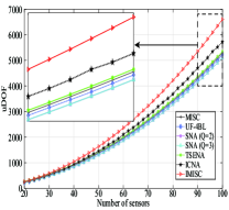
(a) uDOF.

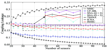
(b) Coupling leakage.

Figure 2: uDOF and coupling leakage versus number of sensors.

V-B Root-Mean-Square Error (RMSE) Performance with various SNR, $|a_{1}|$, and snapshots

In the second example, the RMSE performance in different conditions is considered. All the RMSE results are obtained through 500 trials.

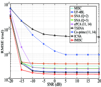
(a) RMSE versus SNR.

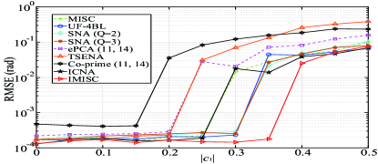
(b) RMSE versus $|a_{1}|$.

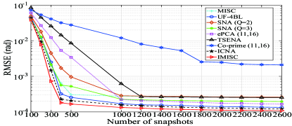
(c) RMSE versus snapshots.

Figure 3: RMSE performance in various conditions.

Firstly, the RMSE performance versus SNR in the presence of coupling is presented. All the SAs have 34 sensors and there are 39 sources in $[-60^{\circ},60^{\circ}]$, and $a_{1}=0.3e^{j\pi/3}$. From Fig. 3(a), it is observed that IMISC has the best performance, due to the longest uDOF and low MC.

Next, the RMSE versus $|a_{1}|$ is investigated. Here, all the SAs consist of $35$ sensors, the number of sources is set to $50$ within azimuth $[-60^{\circ},60^{\circ}]$, SNR= 0 dB, and $|a_{1}|$ varies from 0 to 0.5. As shown in Fig. 3(b), when $|a_{1}|<0.4$, IMISC gives the best performance, while when $|a_{1}|>0.4$, the ICNA and UF-4BL perform better than IMISC.

Finally, the RMSE performance versus the number of snapshots is presented in Fig. 3(c), where all the SAs have 37 sensors, the number of sources is 45 within azimuth $[-60^{\circ},60^{\circ}]$, SNR=0 dB, and $|a_{1}|=0.3$. We can see that the proposed IMISC provides the best performance over snapshots.

VI Conclusion

In this letter, based on the MISC principle, a novel SA structure, termed as IMISC has been proposed. Compared with the MISC array the IMISC array possesses higher uDOF and lower coupling among sensors. The IMISC SA can be uniquely obtained by an inter-element spacing set, which is constrained by the maximum inter-element spacing and the number of sensors. Moreover, the uDOF and the weight function of the IMISC SAs are analyzed in detail. Simulations verify that IMISC can provide a great balance between uDOF and coupling leakage, and hence has better performance in DOA estimation than existing SAs. Future work will focus on how to further reduce the MC among sensors.

Appendix A Consecutive part in the DCA of IMISC

Based on  (13) and due to the symmetric property of DCA, we only need to prove $\mathbb{D}_{\text{IMISC}}^{+}\supset\mathbb{C}_{\text{IMISC}}^{+}$, where $\mathbb{D}_{\text{IMISC}}^{+}$ is the positive set of $\mathbb{D}_{\text{IMISC}}$ and $\mathbb{C}_{\text{IMISC}}^{+}=[1,MQ-\frac{{3{M^{2}}}}{4}-\frac{M}{2}+1]$.

In IMISC, assume that ULA $i$ has the following position set

$$\mathbb{P}_{\text{ULA }i}=\{p_{i}(x),x=1,\dots,Q_{i}\},$$ (20)

where $Q_{i}$ is the number of sensors in ULA $i$. Similarly, setting the position set of ULA $j$ as

$$\mathbb{P}_{\text{ULA }j}=\{p_{j}(y),y=1,\dots,Q_{j}\},$$ (21)

where $Q_{j}$ is the number of sensors in ULA $j$. Then, defining $\mathbb{D}_{i,j}$ as the DCA between ULA $i$ and ULA $j$, which has the following expression

$$\mathbb{D}_{i,j}=\{p_{j}(y)-p_{i}(x),x=1,\dots,Q_{i},y=1,\dots,Q_{j}\}.$$ (22)

In particular, we have

$$\mathbb{D}_{i,i}=\{p_{i}(x),x=1,\dots,Q_{i}\}-p_{i}(1).$$

In IMISC, the number of ULAs is 6, in this regard, $\mathbb{D}_{\text{IMISC}}^{+}$ can be expressed as

$$\mathbb{D}_{\text{IMISC}}^{+}=\bigcup_{i=1}^{5}\mathbb{D}_{i,j},j=i,i+1,\dots,6,$$ (23)

where $\cup$ is the union operator. Based on (12) and (22), some DCA expressions in (23) are provided in (27). The proof of $\mathbb{D}_{\text{IMISC}}^{+}\supset\mathbb{C}_{\text{IMISC}}^{+}$ can be completed by finding consecutive lags within the range $[1,MQ-\frac{{3{M^{2}}}}{4}-\frac{M}{2}+1]$ based (23) and (27) (at the bottom of this page).

Based on (27), one can tell that $\mathbb{D}_{1,2}\cup\mathbb{D}_{1,3}\cup\mathbb{D}_{3,4}\cup\mathbb{D}_{4,5}\cup\mathbb{D}_{5,6}$ can generate consecutive range

$$[1,\frac{M^{2}}{8}-\frac{M}{4}],$$ (24)

and $\mathbb{D}_{1,4}\cup\mathbb{D}_{2,4}\cup\mathbb{D}_{3,4}\cup\mathbb{D}_{4,5}\cup\mathbb{D}_{4,6}\cup\mathbb{D}_{4,4}$ can generate consecutive range

$$[\frac{M^{2}}{8}-\frac{M}{4}+1,MQ-\frac{7M^{2}}{8}-\frac{5M}{4}+3],$$ (25)

and $\mathbb{D}_{1,5}\cup\mathbb{D}_{1,6}\cup\mathbb{D}_{2,5}\cup\mathbb{D}_{2,6}\cup\mathbb{D}_{3,5}\cup\mathbb{D}_{3,6}\cup\mathbb{D}_{1,4}\cup\mathbb{D}_{2,4}\cup\mathbb{D}_{4,6}$ can generate consecutive range

$$[MQ-\frac{7M^{2}}{8}-\frac{5M}{4}+3,MQ-\frac{{3{M^{2}}}}{4}-\frac{M}{2}+1].$$ (26)

Equations (24), (25) and (26) complete the proof.  

$$\mathbb{D}_{\text{1,2}}=\Big{\{}1,2,\dots,\frac{M}{2}\Big{\}},\quad\mathbb{D}_{\text{2,6}}=\Big{\{}MN-\frac{3M^{2}}{4}-M+1+i+j,i=0,1,j=0,2,\dots,\frac{M}{2}-2\Big{\}},$$

$$\mathbb{D}_{\text{1,3}}=\Big{\{}\frac{M}{2}+i+j,i=0,2,\dots,\frac{M}{2}-2,j=(0,1,\dots,\frac{M}{4}-2)(\frac{M}{2}-1)\Big{\}},$$

$$\mathbb{D}_{\text{1,4}}=\Big{\{}\frac{M^{2}}{8}+\frac{M}{4}+2+i+j,i=0,2,\dots,\frac{M}{2}-2,j=(0,1,\dots,N-M-1)(M)\Big{\}},$$

$$\mathbb{D}_{\text{2,4}}=\Big{\{}\frac{M^{2}}{8}+\frac{M}{4}+i+j,i=0,1,j=(0,1,\dots,N-M-1)(M)\Big{\}},$$

$$\mathbb{D}_{\text{3,4}}=\Big{\{}M+i+j,i=(0,1,\dots,\frac{M}{4}-2)(\frac{M}{2}-1),j=(0,1,\dots,N-M-1)(M)\Big{\}},$$

$$\mathbb{D}_{\text{4,5}}=\Big{\{}\frac{M}{2}+1+i+j,i=(0,1,\dots,\frac{M}{4}-2)(\frac{M}{2}+1),j=(0,1,\dots,N-M-1)(M)\Big{\}},$$

$$\mathbb{D}_{\text{4,6}}=\Big{\{}\frac{M^{2}}{8}-\frac{M}{4}+1+i+j,i=0,2,\dots,\frac{M}{2}-2,j=(0,1,\dots,N-M-1)(M)\Big{\}},$$ (27)

$$\mathbb{D}_{\text{5,6}}=\Big{\{}2+i+j,i=0,2,\dots,\frac{M}{2}-2,j=(0,1,\dots,\frac{M}{4}-2)(\frac{M}{2}+1)\Big{\}},$$

$$\mathbb{D}_{\text{1,5}}=\Big{\{}MN-\frac{7M^{2}}{8}-\frac{M}{4}+3+i+j,i=0,2,\dots,\frac{M}{2}-2,j=(0,1,\dots,\frac{M}{4}-2)(\frac{M}{2}+1)\Big{\}},$$

$$\mathbb{D}_{\text{1,6}}=\Big{\{}MN-\frac{3M^{2}}{4}-M+3+i+j,i=0,2,\dots,\frac{M}{2}-2,j=0,2,\dots,\frac{M}{2}-2\Big{\}},$$

$$\mathbb{D}_{\text{2,5}}=\Big{\{}MN-\frac{7M^{2}}{8}-\frac{M}{4}+1+i+j,i=0,1,j=(0,1,\dots,\frac{M}{4}-2)(\frac{M}{2}+1)\Big{\}},$$

$$\mathbb{D}_{\text{3,5}}=\Big{\{}MN-M^{2}+\frac{M}{2}+1+i+j,i=(0,1,\dots,\frac{M}{4}-2)(\frac{M}{2}-1),j=(0,1,\dots,\frac{M}{4}-2)(\frac{M}{2}+1)\Big{\}},$$

$$\mathbb{D}_{\text{3,6}}=\Big{\{}MN-\frac{7M^{2}}{8}-\frac{M}{4}+1+i+j,i=(0,1,\dots,\frac{M}{4}-2)(\frac{M}{2}-1),j=0,2,\dots,\frac{M}{2}-2\Big{\}}.$$

References

• [1] H. L. Van Trees, Optimum Array Processing: Part IV of Detection, Estimation and Modulation Theory. New York: Wiley Interscience, 2002.
• [2] S. H. Talisa, K. W. O’Haver, T. M. Comberiate, M. D. Sharp, and O. F. Somerlock, “Benefits of digital phased array radars,” Proc. IEEE, vol. 104, no. 3, pp. 530–543, Mar. 2016.
• [3] R. O. Nielsen, Sonar Signal Processing. Norwood, MA, USA: Artech House, 1991.
• [4] R. Schmidt, “Multiple emitter location and signal parameter estimation,” IEEE Trans. Antennas Propag., vol. 34, no. 3, pp. 276–280, Mar. 1986.
• [5] P. Chevalier, L. Albera, A. Ferreol, and P. Comon, “On the virtual array concept for higher order array processing,” IEEE Trans. Signal Process., vol. 53, no. 4, pp. 1254–1271, Apr. 2005.
• [6] A. Moffet, “Minimum-redundancy linear arrays,” IEEE Trans. Antennas Propag., vol. AP-16, no. 2, pp. 172–175, Mar. 1968.
• [7] G. S. Bloom and S. W. Golomb, “Applications of numbered undirected graphs,” Proc. IEEE, vol. 65, no. 4, pp. 562–570, Apr. 1977.
• [8] R. T. Hoctor and S. A. Kassam, “The unifying role of the coarray in aperture synthesis for coherent and incoherent imaging,” Proc. IEEE, vol. 78, no. 4, pp. 735–752, Apr. 1990.
• [9] P. Pal and P. P. Vaidyanathan, “Nested arrays: A novel approach to array processing with enhanced degrees of freedom,” IEEE Trans. Signal Process., vol. 58, no. 8, pp. 4167–4181, Aug. 2010.
• [10] P. P. Vaidyanathan and P. Pal, “Sparse sensing with coprime arrays,” in Proc. Asilomar Conf. Signals, Syst., Comput., Pacific Grove, CA, USA, Nov. 2010, pp. 1405–1409.
• [11] P. P. Vaidyanathan and P. Pal, “Sparse sensing with co-prime samplers and arrays,” IEEE Trans. Signal Process., vol. 59, no. 2, pp. 573–586, Feb. 2011.
• [12] P. Pal and P. P. Vaidyanathan, “Coprime sampling and the MUSIC algorithm,” in Proc. Digital Signal Process. Signal Process. Educ. Meeting, Sedona, AZ, USA, Jan. 2011, pp. 289–294.
• [13] X. Wang, Z. Yang, J. Huang and R. C. de Lamare, ”Robust Two-Stage Reduced-Dimension Sparsity-Aware STAP for Airborne Radar With Coprime Arrays,” in IEEE Transactions on Signal Processing, vol. 68, pp. 81-96, 2020.
• [14] W. S. Leite and R. C. d. Lamare, ”List-Based OMP and an Enhanced Model for DOA Estimation With Nonuniform Arrays,” in IEEE Transactions on Aerospace and Electronic Systems, vol. 57, no. 6, pp. 4457-4464, Dec. 2021.
• [15] M. Yang, L. Sun, X. Yuan and B. Chen, “Improved nested array with hole-free DCA and more degrees of freedom,” Electron. Lett., vol. 52, no. 25, pp. 2068–2070, Dec. 2016.
• [16] S. Qin, Y. D. Zhang, and M. G. Amin, “Generalized coprime array configurations for direction-of-arrival estimation,” IEEE Trans. Signal Process., vol. 63, no. 6, pp. 1377–1390, Mar. 2015.
• [17] S. Ren, W. Dong, X. Li, W. Wang, and X. Li, “Extended nested arrays for consecutive virtual aperture enhancement,” IEEE Signal Process. Lett., vol. 27, pp. 575–579, Mar. 2020.
• [18] J. Liu, Y. Zhang, Y. Lu, S. Ren, and S. Cao, “Augmented nested arrays with enhanced DOF and reduced mutual coupling,” IEEE Trans. Signal Process., vol. 65, no. 21, pp. 5549–5563, Nov. 2017.
• [19] C. L. Liu and P. P. Vaidyanathan, “Super nested arrays: Sparse arrays with less mutual coupling than nested arrays,” in Proc. IEEE Int. Conf. Acoust., Speech, Signal Process., Shanghai, China, Mar. 2016, pp. 2976–2980.
• [20] C. L. Liu and P. P. Vaidyanathan, “High order super nested arrays,” in Proc. IEEE Sensor Array Multichannel Signal Process. Workshop, Rio de Janerio, Brazil, Jul. 2016, pp. 1–5.
• [21] C. L. Liu and P. P.Vaidyanathan, “Super nested arrays: Linear sparse arrays with reduced mutual coupling. Part I: Fundamentals,” IEEE Trans. Signal Process., vol. 64, no. 15, pp. 3997-4012, Aug. 2016.
• [22] C. L. Liu and P. P. Vaidyanathan, “Super nested arrays: Linear sparse arrays with reduced mutual coupling. Part II: High-order extensions,” IEEE Trans. Signal Process., vol. 64, no. 16, pp. 4203-4217, Aug. 2016.
• [23] W. Zheng, X. Zhang, Y. Wang, J. Shen, and B. Champagne, “Padded coprime arrays for improved DOA estimation: Exploiting hole representation and filling strategies,” IEEE Trans. Signal Process., vol. 68, pp. 4597–4611, July 2020.
• [24] Z. Peng, Y. Ding, S. Ren, H. Wu, W. Wang, “Coprime nested arrays for DOA estimation: exploiting the nesting property of coprime array,” IEEE Signal Process. Lett., vol. 29, pp. 444–448, Jan. 2022.
• [25] W. Shi, Y. Li, and S. A. Vorobyov, “Low mutual coupling sparse array design using ULA fitting,” in Proc. Int. Conf. Acoust., Speech Signal Process. (ICASSP), Toronto, Canada, Jun. 2021, pp. 2165–2168.
• [26] W. Shi, S. A. Vorobyov and Y. Li “ULA Fitting for Sparse Array Design,” IEEE Trans. Signal Process., vol. 69, no. 21, pp. 6431–6447, Nov. 2021.
• [27] Z. Zheng, W. Q. Wang, Y. Kong, and Y. D. Zhang, “MISC array: A new sparse array design achieving increased degrees of freedom and reduced mutual coupling effect,” IEEE Trans. Signal Process., vol. 67, no. 7, pp. 1728–1741, Apr. 2019.
• [28] B. Friedlander and A. J. Weiss, “Direction finding in the presence of mutual coupling,” IEEE Trans. Antennas Propag., vol. 39, no. 3, pp. 273–284, Mar. 1991.
• [29] Z. Ye, J. Dai, X. Xu, and X. Wu, “DOA estimation for uniform linear array with mutual coupling,” IEEE Trans. Aerosp. Electron. Syst., vol. 45, no. 1, pp. 280–288, Jan. 2009.
• [30] R. C. de Lamare and R. Sampaio-Neto, “Adaptive Reduced-Rank MMSE Filtering with Interpolated FIR Filters and Adaptive Interpolators”, IEEE Signal Processing Letters, vol. 12, no. 3, March, 2005.
• [31] R. C. de Lamare and R. Sampaio-Neto, “Adaptive Reduced-Rank Processing Based on Joint and Iterative Interpolation, Decimation and Filtering”, IEEE Transactions on Signal Processing, vol. 57, no. 7, July 2009, pp. 2503 - 2514.
• [32] R. Fa, R. C. de Lamare, and L. Wang, “Reduced-Rank STAP Schemes for Airborne Radar Based on Switched Joint Interpolation, Decimation and Filtering Algorithm,” IEEE Transactions on Signal Processing, vol.58, no.8, Aug. 2010, pp.4182-4194.
• [33] L. Qiu, Y. Cai, R. C. de Lamare and M. Zhao, “Reduced-Rank DOA Estimation Algorithms Based on Alternating Low-Rank Decomposition,” IEEE Signal Processing Letters, vol. 23, no. 5, pp. 565-569, May 2016.