Improving knockoffs with conditional calibration

Abstract

The knockoff filter of Barber and Candès (2015) is a flexible framework for multiple testing in supervised learning models, based on introducing synthetic predictor variables to control the false discovery rate (FDR). Using the conditional calibration framework of Fithian and Lei (2022), we introduce the calibrated knockoff procedure, a method that uniformly improves the power of any knockoff procedure. We implement our method for fixed-$X$ knockoffs and show theoretically and empirically that the improvement is especially notable in two contexts where knockoff methods can be nearly powerless: when the rejection set is small, and when the structure of the design matrix prevents us from constructing good knockoff variables. In these contexts, calibrated knockoffs even outperform competing FDR-controlling methods like the (dependence-adjusted) Benjamini–Hochberg procedure in many scenarios.

1 Introduction

The Gaussian linear regression model is one of the most versatile and best-studied models in statistics, with myriad applications in experimental analysis, causal inference, and machine learning. In modern applications, there are commonly many explanatory variables, and we suspect that most of them have little to do with the response, i.e. that the true coefficient vector is (approximately) sparse. In such problems, multiple hypothesis testing methods are a natural tool for discovering a small number of variables with nonzero coefficients in the sea of noise variables, while controlling some error measure such as the false discovery rate (FDR), introduced by Benjamini and Hochberg (1995).

At present, however, the multiple testing literature offers practitioners little clarity regarding how they ought to perform the inference. There are at least two well-known methods for multiple testing with FDR control: the (fixed-$X$) knockoff filter of Barber and Candès (2015) and the Benjamini–Hochberg (BH) procedure of Benjamini and Hochberg (1995) (recently modified by Fithian and Lei (2022) to ensure provable FDR control in linear regression among other problems with dependent $p$-values). Knockoffs and BH use radically different approaches and can return very different rejection sets on the same data, and it is not uncommon for one method to dramatically outperform the other, depending on the problem context. For example, Example 1.1 illustrates a simple problem setting where BH has much higher power at FDR level $\alpha=0.05$, but the knockoff filter recovers and outperforms BH at level $\alpha=0.2$. In particular, the knockoff filter suffers from a so-called threshold phenomenon, explained in Section 2.1, that makes it nearly powerless when the number of discernibly non-null variables is smaller than $1/\alpha$, making it a risky choice for an analyst who aims for more stringent FDR control. In problems with enough rejections to avoid this issue, however, the knockoff filter often shines, since it can use efficient estimation methods like the lasso (Tibshirani, 1996) to guide its prioritization of variables.

In this work, we propose a new method, the calibrated Knockoff procedure (cKnockoff), which uniformly improves the knockoff filter’s power while achieving finite-sample FDR control. Our method augments the rejection set of any knockoff procedure using a “fallback test” for each variable that is not selected by knockoffs. To set the power of the fallback tests without violating FDR control, we use the conditional calibration framework proposed in Fithian and Lei (2022). With exactly the same assumption and data, cKnockoff is strictly more powerful than knockoffs in every problem instance, but the power gain is especially large in problems with a small number of non-null variables, resolving the threshold phenomenon while retaining the knockoff filter’s advantages.

Although the majority of this paper is focused on fixed-$X$ knockoffs in the Gaussian linear model, our cKnockoff method applies with only minor modifications to the model-$X$ knockoffs (Candès et al., 2018) (need to mention that it will require different computational tricks). As a variant of the originally proposed fixed-$X$ knockoffs, the model-$X$ knockoffs employs the same core technique but adopts fundamentally different assumptions and language. They require no model assumption on the relationship between the explanatory variables and the outcome but assume the joint distribution of the explanatory variables is known. We describe our cKnockoff method for model-$X$ knockoffs in Section 5.

1.1 Multiple testing in the Gaussian linear model

We consider the linear model relating an observed response vector $\boldsymbol{y}=(y_{1},\ldots,y_{n})^{\mkern-1.5mu\mathsf{T}}$ to fixed explanatory variables $\boldsymbol{X}_{j}=(X_{1j},\ldots,X_{nj})^{T}$, for $j=1,\ldots,m$ via

$$\boldsymbol{y}=\sum_{j=1}^{m}\boldsymbol{X}_{j}\beta_{j}+\boldsymbol{\varepsilon}=\boldsymbol{X}\boldsymbol{\beta}+\boldsymbol{\varepsilon},\quad\boldsymbol{\varepsilon}\sim\mathcal{N}(\boldsymbol{0},\sigma^{2}\boldsymbol{I}_{n}),$$ (1)

where the design matrix $\boldsymbol{X}\in\mathbb{R}^{n\times m}$ has $\boldsymbol{X}_{j}$ as its $j$th column. Both the coefficient vector $\boldsymbol{\beta}=(\beta_{1},\ldots,\beta_{m})^{\mkern-1.5mu\mathsf{T}}$ and the error variance $\sigma^{2}$ are assumed to be unknown. We assume throughout that $m<n$, and that $X$ has full column rank, ensuring that $\boldsymbol{\beta}$ and $\sigma^{2}$ are identifiable.

A central inference question in this model is whether a given variable $\boldsymbol{X}_{j}$ helps to explain the response, after adjusting for the other variables. Formally, we will study the problem of testing the hypothesis $H_{j}:\beta_{j}=0$ for each variable $\boldsymbol{X}_{j}$ simultaneously, while controlling the FDR.

Let $\mathcal{H}_{0}=\{j:H_{j}\mbox{ is true}\}$ be the index set of true null hypotheses and $m_{0}=|\mathcal{H}_{0}|$ be the number of nulls; we say $\boldsymbol{X}_{j}$ is a null variable if $j\in\mathcal{H}_{0}$. For a multiple testing procedure with rejection set $\mathcal{R}\subset\{1,\ldots,m\}$, the false discovery proportion (FDP) and FDR are defined respectively as

$$\textnormal{FDP}(\mathcal{R})=\frac{|\mathcal{R}\cap\mathcal{H}_{0}|}{|\mathcal{R}|\vee 1},\quad\textnormal{FDR}=\mathbb{E}[\textnormal{FDP}].$$

We write $R=|\mathcal{R}|$ and $V=|\mathcal{R}\cap\mathcal{H}_{0}|$ for the number of rejections and false rejections respectively. Our goal is to control FDR at a pre-specified threshold $\alpha$ while achieving a power as high as possible. Throughout this paper we define power in terms of the true positive rate (TPR), defined as the expectation of the true positive proportion (TPP), the fraction of the $m_{1}=m-m_{0}$ non-null hypotheses rejected:

$$\textnormal{TPP}(\mathcal{R})=\frac{|\mathcal{R}\cap\mathcal{H}_{0}^{\mathsf{c}}|}{m_{1}},\quad\textnormal{TPR}=\mathbb{E}[\textnormal{TPP}].$$

1.2 Knockoff methods

A traditional approach to multiple testing would start with the usual two-sided $t$-test statistics $|\hat{\beta}_{j}|/\hat{\sigma}$, which are calculated from the ordinary least squares (OLS) estimator and the unbiased estimator of the error variance

$$\hat{\boldsymbol{\beta}}=(\boldsymbol{X}^{\mkern-1.5mu\mathsf{T}}\boldsymbol{X})^{-1}\boldsymbol{X}^{\mkern-1.5mu\mathsf{T}}\boldsymbol{y},\quad\text{ and }\hat{\sigma}^{2}=\textnormal{RSS}/(n-m),$$

where $\textnormal{RSS}=\|\boldsymbol{y}-\boldsymbol{X}\hat{\boldsymbol{\beta}}\|_{2}^{2}$ is the residual sum of squares. Such $t$-tests are uniformly most powerful unbiased for the individual hypotheses. Then an appropriate multiplicity correction is applied to their corresponding $p$-values. The celebrated Benjamini–Hochberg procedure (BH), the best-known FDR-controlling method, orders the $p$-values from smallest to largest $p_{(1)}\leq\cdots\leq p_{(m)}$, and rejects

$$\mathcal{R}^{{\textnormal{BH}}}=\left\{j:p_{j}\leq\frac{\alpha R^{{\textnormal{BH}}}}{m}\right\},\quad\text{ where }\;\;R^{{\textnormal{BH}}}=\max\left\{r:\;p_{(r)}\leq\frac{\alpha r}{m}\right\}.$$

While BH does not provably control FDR in this context due to the dependence between $p$-values, a corrected version called the dependence-adjusted BH procedure (dBH) does, while achieving nearly identical power (Fithian and Lei, 2022).

The knockoff filter, described below in Section 2.1, is a flexible class of methods that take a radically different approach, completely bypassing the $t$-tests. Instead, these methods introduce a “knockoff” variable $\tilde{\boldsymbol{X}}_{j}$ to serve as a negative control for each real predictor variable $\boldsymbol{X}_{j}$, and then apply a learning algorithm to rank the $2m$ variables according to some importance measure in the model. The knockoffs are constructed to ensure that, under $H_{j}$, $\boldsymbol{X}_{j}$ and $\tilde{\boldsymbol{X}}_{j}$ are indistinguishable in an appropriate sense.

A major advantage of the knockoffs framework is that it requires no additional assumptions beyond the standard Gaussian linear model (1), and controls FDR in finite samples for any parameters $\beta$ and $\sigma^{2}$, and fixed design matrix $X$. This distinguishes knockoffs from many methods for inference in higher-dimensional settings, which typically require stronger assumptions including sparsity of $\beta$ and distribution of $X$, and deliver asymptotic guarantees for inference on single parameters rather than finite-sample simultaneous inference on all variables with FDR control (Zhang and Zhang, 2014; Van de Geer et al., 2014; Javanmard and Montanari, 2014; Ning and Liu, 2017; Shah and Peters, 2020; Shah and Bühlmann, 2023).

Knockoff methods enjoy substantially higher power than BH and dBH in some scenarios while struggling in others, with the relative performance depending on the problem dimensions, the structure of the design matrix, and the true $\beta$ vector, among other considerations, as we see next.

Example 1.1 (MCC-Block).

Consider a drug company doing $k=1,\ldots,K$ independent clinical trials. Each trial targets a disease and there are $G$ different candidate drugs for it. In each trial, we have one common control group receiving no treatment and $G$ treatment groups each receiving a different drug. All groups are assumed to have the same number of patients $r$ for simplicity.

Formally, for patient $i$ in treatment group $g$ in trial $k$, we observe the outcome

$$z_{k,g,i}=\mu_{k}+\delta_{k,g}+\varepsilon_{k,g,i},$$

where $\mu_{k}$ represents the common “baseline” outcome in trial $k$, $\delta_{k,g}$ is the treatment effect of drug $g$ in trial $k$, and $\varepsilon_{k,g,i}\overset{\textnormal{i.i.d.}}{\sim}N(0,\sigma^{2})$ is the independent individual noise from each patient. Likewise, patient $i$ from the control group (group index denoted as $g=0$) has outcome

$$z_{k,0,i}=\mu_{k}+\varepsilon_{k,0,i}.$$

We are interested in if the treatment effect $\delta_{k,g}=0$ for all drugs.

Example 1.1 can be equivalently expressed as a linear model of the form (1) with $m=KG$ variables and $n=K(r(G+1)-1)$ independent observations, where $\beta_{j}=\delta_{k,g}$ for $j=(k-1)G+g$; see Appendix E.1 for details. The OLS estimator for $\delta_{k,g}$ is easily shown to be

$$\hat{\delta}_{k,g}=\overline{z}_{k,g}-\overline{z}_{k,0}=\delta_{k,g}+\overline{\varepsilon}_{k,g}-\overline{\varepsilon}_{k,0}$$ (2)

where $\overline{z}_{k,g}$ and $\overline{z}_{k,0}$ respectively represent the sample means for the $g$th treatment group and the control group in trial $k$, and $\overline{\varepsilon}_{k,g}$ and $\overline{\varepsilon}_{k,0}$ are defined similarly.

To test any individual hypothesis, the two-sided $t$-test using $t$-statistic $\sqrt{r/2\hat{\sigma}^{2}}\cdot\delta_{k,g}$ seems virtually unassailable. As a result, it would be quite natural to apply the BH method, or its close cousin dBH, with the $t$-test $p$-values. However, BH may be sub-optimal compared to knockoffs in this problem. To understand why, we must carefully consider the implications of sparsity: that we may expect $\delta_{k,g}\approx 0$ for the vast majority of drugs. Therefore if in trial $k$ we observe

$$\hat{\delta}_{k,1}\approx 0\quad\text{and}\quad\hat{\delta}_{k,2},\hat{\delta}_{k,3},\ldots,\hat{\delta}_{k,G}\in[-3,-1],$$

it wouldn’t imply that all drugs except $1$ are effective under the sparsity assumption. Instead, this would be a strong hint for $\delta_{k,1}>1$. That is, the nonzero $\hat{\delta}_{k,g}$ are caused by a common positive noise $\overline{\varepsilon}_{k,0}$. While pharmaceutical researchers would be confident in sparsity, the OLS estimator that forms the backbone of the BH method does not utilize the sparsity in any way, since the distributions of the $j$th $t$-statistic, $\sqrt{r/2\hat{\sigma}^{2}}\cdot\hat{\delta}_{k,g}$ and its $p$-value depend only on $\delta_{k,g}/\sigma$.

If $\boldsymbol{\beta}$ is sparse, however, we should be able to exploit the sparsity to improve our estimator of $\boldsymbol{\beta}$, for example by using the lasso estimator of Tibshirani (1996), defined by

$$\hat{\boldsymbol{\beta}}^{\lambda}=\underset{\boldsymbol{\beta}\in\mathbb{R}^{m}}{\text{argmin}}\;\;\frac{1}{2}\left\|\boldsymbol{y}-\boldsymbol{X}\boldsymbol{\beta}\right\|_{2}^{2}+\lambda\cdot\left\|\boldsymbol{\beta}\right\|_{1}.$$ (3)

The power of exploiting sparsity in lasso transfers to knockoffs while the FDR is still controlled. As shown in Figure 1, a version of the knockoff filter based on the lasso can outperform the OLS-based BH method, but its superior performance is only observed in this instance for $\alpha=0.2$. For smaller $\alpha$ values, a specific drawback of knockoffs — ironically, that knockoff methods break down when the coefficient vector is too sparse — prevents the method from realizing its potential. This drawback is resolved by our calibrated knockoff method, the main subject of this work.

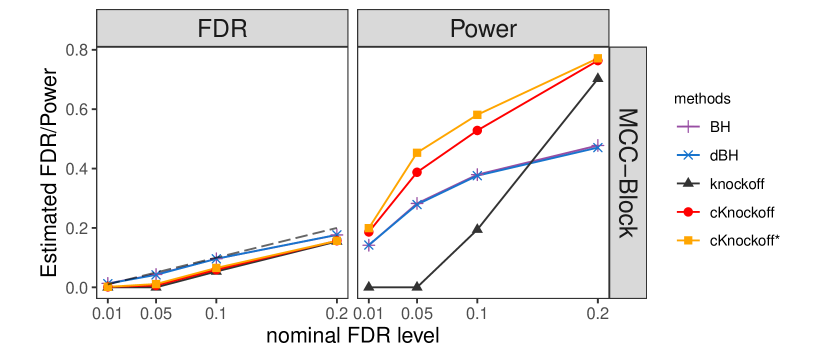
Figure 1: Performance of several multiple testing methods for the MCC-Block problem with $K=200$, $G=5$, $r=3$, and $m_{1}=10$, for varying FDR significance levels, $\alpha=0.01,0.05,0.1,$ and $0.2$. The knockoff method using lasso-based LCD feature statistics outperforms BH by a wide margin when $\alpha=0.2$ by successfully exploiting sparsity, but it fails for smaller values of $\alpha$ due to the threshold phenomenon. The cKnockoff method described in this paper outperforms both BH and knockoffs.

1.3 Outline and contributions

In this work, we propose the calibrated Knockoff procedure (cKnockoff), a method that controls finite-sample FDR under the same assumption as knockoffs. Our method augments the rejection set of any knockoff procedure, uniformly improving its power by means of a fallback test that allows for selection of variables not selected by knockoffs.

Our fallback test takes a very simple form. For any reasonable test statistic $T_{j}(\boldsymbol{y})$ for the significance of $X_{j}$, our framework will compute a data-adaptive threshold $\hat{c}_{j}(\boldsymbol{y})$, and reject $H_{j}$ for any $j$ which has $T_{j}(\boldsymbol{y})\geq\hat{c}_{j}(\boldsymbol{y})$, beside the knockoff rejection set. That is,

$$\mathcal{R}^{{\textnormal{cKn}}}\;=\;\mathcal{R}^{{\textnormal{Kn}}}\,\cup\,\{j:\;T_{j}(\boldsymbol{y})\geq\hat{c}_{j}(\boldsymbol{y})\},$$

where $\mathcal{R}^{{\textnormal{Kn}}}$ and $\mathcal{R}^{{\textnormal{cKn}}}$ are respectively the rejection sets for the baseline and calibrated knockoff methods.

The calculation of $\hat{c}_{j}$ involves a lot of mathematical details though. As a high-level description, we figure out the gap between the FDR “budget” $\alpha$ and the actual FDR of knockoffs. Then the budget gap is distributed to each variable via $\hat{c}_{j}$ through a conditional FDR calibration method of Fithian and Lei (2022), which we review in more detail in Section 2.3. In brief, define $S_{j}=(\boldsymbol{X}_{-j}^{\mkern-1.5mu\mathsf{T}}\boldsymbol{y},\;\|\boldsymbol{y}\|_{2}^{2})$, the complete sufficient statistic for the submodel described by $H_{j}$. Then under $H_{j}$, the distribution of $\boldsymbol{y}$ given $S_{j}$ is known so that, for any fallback test threshold $c_{j}$, we can calculate the resulting conditional FDR contribution of $H_{j}$, defined as

$$\textnormal{FDR}_{j}(\mathcal{R}^{{\textnormal{cKn}}}\mid S_{j})\;\coloneqq\;\mathbb{E}_{H_{j}}\left[\frac{\mathbf{1}\left\{j\in\mathcal{R}^{{\textnormal{cKn}}}\right\}}{\left|\mathcal{R}^{{\textnormal{cKn}}}\right|\vee 1}\;\Big{|}\;S_{j}\right]\;\leq\;\mathbb{E}_{H_{j}}\left[\frac{\mathbf{1}\left\{j\in\mathcal{R}^{\textnormal{Kn}}\right\}\vee\mathbf{1}\left\{T_{j}\geq c_{j}\right\}}{\left|\mathcal{R}^{{\textnormal{Kn}}}\cup\{j\}\right|}\;\Big{|}\;S_{j}\right].$$

We will choose the threshold $\hat{c}_{j}(S_{j}(\boldsymbol{y}))$ to set the last expression equal to the FDR budget that we distribute to variable $j$.

Because the cKnockoff rejection set always includes the knockoff rejection set and sometimes exceeds it, the method is uniformly more powerful than knockoffs. We find in simulations that the power gain is especially large when the true $\boldsymbol{\beta}$ vector is very sparse, in particular when we do not have $m_{1}\gg 1/\alpha$.

The only downside of cKnockoff is the additional computation it requires. To reduce this burden, we only carry out the fallback test on hypotheses that appear promising, and we use a conservative algorithm to speed the fallback test calculation. We prove that these speedup techniques do not inflate the FDR, and we find numerically that the computation time of our implementation is a small multiple of the knockoff computation time, which is further improved when parallel computing is available.

Section 2 reviews the basics of knockoffs and conditional calibration, and Section 3 defines our method in full detail. Section 4 gives more detail about how we implement the fallback test for a given variable, using a single Monte Carlo integral. Section 5 describes the calibrated knockoffs in the model-$X$ setting. Sections 6–8 illustrate our method’s performance on selected simulation scenarios, in addition to the HIV data from the original knockoff paper (Barber and Candès, 2015), and Section 9 concludes.

2 Review: knockoffs and conditional calibration

2.1 Knockoffs: a flexible framework

This section reviews the elements of knockoffs and conditional calibration. Our focus is on fixed-$X$ knockoffs, the original version of the knockoff filter proposed in Barber and Candès (2015) for the Gaussian linear model with fixed design. In this setting, the requisite “indistinguishability” is defined by the pairwise correlations between variables. Specifically, the knockoff design matrix $\tilde{\boldsymbol{X}}=(\tilde{\boldsymbol{X}}_{1},\ldots,\tilde{\boldsymbol{X}}_{m})\in\mathbb{R}^{n\times m}$ must satisfy

$$\tilde{\boldsymbol{X}}^{\mkern-1.5mu\mathsf{T}}\tilde{\boldsymbol{X}}=\boldsymbol{X}^{\mkern-1.5mu\mathsf{T}}\boldsymbol{X},\quad\text{ and }\;\;\boldsymbol{X}^{\mkern-1.5mu\mathsf{T}}\tilde{\boldsymbol{X}}=\boldsymbol{X}^{\mkern-1.5mu\mathsf{T}}\boldsymbol{X}-\boldsymbol{D},$$ (4)

for some diagonal matrix $\boldsymbol{D}$. Following Barber and Candès (2015), we require $n\geq 2m$; in some cases we will require further that $n\geq 2m+1$ so that $\sigma^{2}$ is identifiable in the augmented linear model with design matrix $\boldsymbol{X}_{+}=(\boldsymbol{X},\tilde{\boldsymbol{X}})\in\mathbb{R}^{n\times 2m}$.

There are many ways to implement knockoffs, but every knockoff method yields common intermediate outputs called feature statistics $W_{1},\ldots,W_{m}\in\mathbb{R}$ which are inputs to an ordered multiple testing algorithm called Selective SeqStep, also proposed in Barber and Candès (2015). The absolute value $|W_{j}|$ roughly quantifies how much overall importance the learning algorithm assigns to the pair $\{\boldsymbol{X}_{j},\tilde{\boldsymbol{X}}_{j}\}$, while the sign ${\textnormal{sgn}}(W_{j})$ is positive if the algorithm assigns greater importance to $\boldsymbol{X}_{j}$ than $\tilde{\boldsymbol{X}}_{j}$, and negative otherwise. Formally, each $W_{j}$ must be a function of $\boldsymbol{X}_{+}^{\mkern-1.5mu\mathsf{T}}\boldsymbol{X}_{+}$ and $\boldsymbol{X}_{+}^{\mkern-1.5mu\mathsf{T}}\boldsymbol{y}$ (the sufficiency condition) and $W_{j}$ must have the same absolute value but opposite sign whenever we swap $\boldsymbol{X}_{j}$ with $\tilde{\boldsymbol{X}}_{j}$ (the anti-symmetry condition).

The two most popular feature statistics in practice, proposed by Barber and Candès (2015) and Candès et al. (2018) respectively, are both based on the Lasso estimator for the augmented model:

$$\hat{\boldsymbol{\beta}}^{\lambda}=\underset{\boldsymbol{\beta}\in\mathbb{R}^{2m}}{\text{argmin}}\;\;\frac{1}{2}\left\|\boldsymbol{y}-\boldsymbol{X}_{+}\boldsymbol{\beta}\right\|_{2}^{2}+\lambda\cdot\left\|\boldsymbol{\beta}\right\|_{1}.$$

The lasso signed-max (LSM) statistics are defined by variables’ entry points on the regularization path:

$$W_{j}^{\text{LSM}}=(\lambda_{j}^{*}\vee\lambda_{j+m}^{*})\cdot{\textnormal{sgn}}(\lambda_{j}^{*}-\lambda_{j+m}^{*}),\quad\text{ for }\;\;\lambda_{j}^{*}=\sup\left\{\lambda:\;\hat{\beta}_{j}^{\lambda}\neq 0\right\},$$ (5)

while the lasso coefficient-difference (LCD) statistics are defined by the lasso estimator for a fixed $\lambda$:

$$W_{j}^{\text{LCD}}=|\hat{\beta}_{j}^{\lambda}|-|\hat{\beta}_{j+m}^{\lambda}|.$$ (6)

If $\beta_{j}^{\lambda}=\beta_{j+m}^{\lambda}=0$, then $W_{j}^{\text{LCD}}=0$. For the simulations in this paper, we use a minor modification of $\boldsymbol{W}^{\text{LCD}}$ that breaks ties using the variables’ correlations with the lasso residuals

$$\boldsymbol{r}^{\lambda}=\boldsymbol{y}-\boldsymbol{X}_{+}\hat{\boldsymbol{\beta}}^{\lambda}.$$ (7)

Formally, we define the LCD with tiebreaker (LCD-T) statistics as

$$W_{j}^{\text{LCD-T}}\;=\;\begin{cases}W_{j}^{\text{LCD}}+2\lambda\,\text{sgn}(W_{j}^{\text{LCD}})&\text{if }W_{j}^{\text{LCD}}\neq 0\\[5.0pt] |\boldsymbol{X}_{j}^{\mkern-1.5mu\mathsf{T}}\boldsymbol{r}^{\lambda}|-|\tilde{\boldsymbol{X}}_{j}^{\mkern-1.5mu\mathsf{T}}\boldsymbol{r}^{\lambda}|&\text{otherwise.}\end{cases}$$ (8)

Applying the Karush–Kuhn–Tucker (KKT) condition, it is easy to verify that $|W_{j}^{\text{LCD-T}}|>2\lambda$ if and only if $W_{j}^{\text{LCD}}\neq 0$.

The sufficiency and antisymmetry conditions can be relaxed slightly. If $n\geq 2m+1$, then $W$ can also take as input the unbiased variance estimator $\tilde{\sigma}^{2}=\|\boldsymbol{r}^{0}\|_{2}^{2}/(n-2m)$, which is independent of $\boldsymbol{X}_{+}^{\mkern-1.5mu\mathsf{T}}\boldsymbol{y}$ (Li and Fithian, 2021). This can help us to select $\lambda$ in (6); we find that $\lambda=2\tilde{\sigma}$ is a practical choice , where the predictor variables are standardized to have a unit norm.

Knockoff methods’ FDR control guarantee arises from a crucial stochastic property of the feature statistics: conditional on their absolute values $|\boldsymbol{W}|=(|W_{1}|,\ldots,|W_{m}|)$, the signs for null variables are independent Rademacher random variables:

$${\textnormal{sgn}}(W_{j})\,\mid\,|W_{j}|,\,\boldsymbol{W}_{-j}\;\stackrel{{\scriptstyle H_{j}}}{{\sim}}\;\textnormal{Unif}\{-1,+1\},$$ (9)

where $\boldsymbol{W}_{-j}$ encodes all entries other than $W_{j}$. To avoid trivialities, we assume all $W_{j}\neq 0$ and $W_{i}\neq W_{j}$ for any $i\neq j$.

Once the feature statistics are calculated, Selective SeqStep rejects $H_{j}$ if $W_{j}\geq\widehat{w}$, for an adaptive rejection threshold $\widehat{w}\geq 0$ that is based on a running estimator of FDP:

$$\widehat{w}=\min\left\{w\geq 0:\;\widehat{\textnormal{FDP}}(w)\leq\alpha\right\},\quad\text{for }\;\widehat{\textnormal{FDP}}(w)=\frac{1+|\{j:\;W_{j}\leq-w\}|}{|\{j:\;W_{j}\geq w\}|},$$ (10)

where $\widehat{w}=\infty$ (no rejections) if $\widehat{\textnormal{FDP}}(w)>\alpha$ for all $w$. Let $\mathcal{R}^{{\textnormal{Kn}}}=\{W_{j}\geq\widehat{w}\}$ denote the knockoff rejection set. This rejection rule controls FDR at level $\alpha$ whenever the feature statistics satisfy (9), as Section 3.4 discusses in detail. Appendix A.1 includes a proof of (9) for fixed-$X$ knockoffs.

2.2 Two limitations of knockoffs

Despite its deft exploitation of sparsity, the fixed-$X$ knockoff filter has two major limitations that can inhibit its performance in certain settings. One limitation, reflected in Figure 1, is the so-called threshold phenomenon: because the denominator of $\widehat{\textnormal{FDP}}_{w}$ is the size of the candidate rejection set, we cannot make any rejections at all unless we have $R\geq 1/\alpha$. For example, if $\alpha=0.1$, we must make at least $10$ rejections or none at all, even if several $p$-values lie well below the Bonferroni threshold $\alpha/m$. Even when the number of potential rejections is above the $1/\alpha$ threshold, the FDP estimator can be highly variable and upwardly biased, adversely affecting the method’s power and stability.

Some recent proposals ameliorate this limitation by generating multiple negative controls (Gimenez and Zou, 2019; Emery and Keich, 2019; Nguyen et al., 2020). However, they come at the price of a higher correlation between the original variables and negative controls and a noisier ordering of the variables passed into the Selective Seqstep filter, both of which potentially lead to reduced power (Nguyen et al., 2020). Another proposal by Sarkar and Tang (2021) views fixed-$X$ knockoffs as “splitting” the data into two unbiased estimators of $\beta$, one of which has independent coordinates, and applies a hybrid data-splitting method. This proposal can also mitigate the threshold phenomenon, but is often less powerful than knockoffs. By contrast, our calibrated knockoff method is always more powerful than a baseline knockoff method, and we find in simulations that it usually outperforms both multiple knockoffs and the method of Sarkar and Tang (2021) as well.

A second issue is the whiteout phenomenon discussed by Li and Fithian (2021), who prove finite-sample bounds on the power of any fixed-$X$ knockoff method in terms of the eigenvalues and eigenvectors of $X^{\mkern-1.5mu\mathsf{T}}X$, and the coefficient vector $\beta$. When the eigenstructure is unfavorable, we may be forced to make all but a few knockoff variables very highly correlated with their real variable counterparts, and as a result, ${\textnormal{sgn}}(W_{j})$ can be very noisy even for strong signal variables, severely biasing $\widehat{\textnormal{FDP}}_{w}$ upwards. The MCC problem (Example 1.1 with $K=1$) is a prototypical example exhibiting the whiteout phenomenon, and Li and Fithian (2021) prove that in large MCC problems, even the Bonferroni method is dramatically more powerful than the best possible knockoff method. More prosaically, even when the results of Li and Fithian (2021) do not cause catastrophic failure, the knockoff variables still tend to interfere with one another, degrading each other’s quality. Multiple knockoff methods tend to exacerbate these problems. As we will see, calibrated knockoffs partially address this issue, delivering high power under some circumstances, but giving limited performance gains in other settings.

Note that these limitations do not conflict with recent theoretical analyses establishing positive results in regimes where the design matrix is well-conditioned and the number of non-nulls diverges; see e.g. Weinstein et al. (2017); Fan et al. (2019); Liu and Rigollet (2019); Wang and Janson (2020).

2.3 Conditional calibration and dBH

Fithian and Lei (2022) introduced a novel technique called conditional calibration for proving and achieving FDR control under dependence. They begin by decomposing the FDR into the contributions from each null hypothesis:

$$\textnormal{FDR}(\mathcal{R})\;=\;\sum_{j\in\mathcal{H}_{0}}\textnormal{FDR}_{j}(\mathcal{R}),\quad\text{ where }\;\;\textnormal{FDR}_{j}(\mathcal{R})\;=\;\mathbb{E}_{H_{j}}\left[\frac{\mathbf{1}\{j\in\mathcal{R}\}}{R\vee 1}\right],$$ (11)

and propose controlling each FDR contribution at level $\alpha/m$, so that $\textnormal{FDR}\leq\alpha m_{0}/m\leq\alpha$.

Just as we decomposed the FDR into the contributions from each null hypothesis, we can likewise decompose the FDP as

$$\textnormal{FDP}\;=\;\sum_{j\in\mathcal{H}_{0}}\textnormal{DP}_{j},\quad\text{ where }\;\;\textnormal{DP}_{j}(\mathcal{R})\;=\;\frac{\mathbf{1}\{j\in\mathcal{R}\}}{R\vee 1}\;=\;\frac{\mathbf{1}\{j\in\mathcal{R}\}}{\left|\mathcal{R}\cup\{j\}\right|}.$$ (12)

We will call $\textnormal{DP}_{j}$ the realized discovery proportion for $H_{j}$; then $\textnormal{FDR}_{j}=\mathbb{E}_{H_{j}}[\textnormal{DP}_{j}]$. Note that $\textnormal{DP}_{j}$ only contributes to FDP if $H_{j}$ is true, but it is a well-defined statistic whether $H_{j}$ is true or false.

To control $\textnormal{FDR}_{j}$ at level $\alpha/m$, Fithian and Lei (2022) first condition on a sufficient statistic $S_{j}$ for the submodel described by $H_{j}$. By the sufficiency of $S_{j}$, the conditional expectation $\mathbb{E}_{H_{j}}[\textnormal{DP}_{j}(\mathcal{R})\mid S_{j}]$ can be calculated for any rejection rule $\mathcal{R}$; as a result, a rejection rule with a tuning parameter can also be calibrated to control the conditional expectation at $\alpha/m$.

In particular, the dBH procedure thresholds the BH-adjusted $p$-value for $H_{j}$ at an adaptive rejection cutoff $\hat{c}^{\textnormal{dBH}}_{j}$. When $\hat{c}^{\textnormal{dBH}}_{j}\geq\alpha$, dBH is more liberal than BH (at least concerning $H_{j}$), and when $\hat{c}^{\textnormal{dBH}}_{j}\leq\alpha$ it is more conservative.

3 Our method: calibrated knockoffs

3.1 Conditional calibration for knockoffs

Our method provides an additional rejection set to the knockoff procedure. We reject any hypothesis that is rejected by knockoff or by a fallback test with a data-adaptive threshold. The FDR is guaranteed to be controlled via conditional calibration.

Formally, our calibrated knockoff procedure (cKnockoff) rejects $H_{j}$ if $j$ is in the index set

$$\mathcal{R}^{{\textnormal{cKn}}}\;=\;\mathcal{R}^{{\textnormal{Kn}}}\,\cup\,\{j:\;T_{j}(\boldsymbol{y})\geq\hat{c}_{j}(\boldsymbol{y})\},$$ (13)

where $T_{j}(\boldsymbol{y})$ is any test statistic and $\hat{c}_{j}(\boldsymbol{y})$ is a data-adaptive threshold that is calibrated to achieve FDR control. For notational convenience, we will suppress the dependence on $\boldsymbol{y}$ when no confusion can arise. We describe $T_{j}$ and $\hat{c}_{j}$ in detail next.

Ingredient 1: The fallback test statistics. The test statistic $T_{j}$ can be chosen arbitrarily by the analyst, with larger values representing stronger evidence against the null. To simplify the presentation, we assume that $T_{j}$ is non-negative and continuously distributed. Our implementation of cKnockoff uses a modified version of the usual $t$-statistic that replaces the OLS residuals with residuals from a lasso model (see Section 3.3), but a casual reader can just think of $T_{j}$ as the absolute value of the usual $t$-statistic.

Ingredient 2: The fallback test threshold. The rejection threshold $\hat{c}_{j}$ is calibrated to ensure FDR control. Specifically, if we set the fallback test threshold at $c_{j}$, then

$$\textnormal{DP}_{j}(\mathcal{R}^{\textnormal{cKn}})\;=\;\frac{\mathbf{1}\left\{j\in\mathcal{R}^{\textnormal{Kn}}\right\}\vee\mathbf{1}\left\{T_{j}\geq c_{j}\right\}}{\left|\mathcal{R}^{\textnormal{cKn}}\cup\{j\}\right|}\;\leq\;\frac{\mathbf{1}\left\{j\in\mathcal{R}^{\textnormal{Kn}}\right\}\vee\mathbf{1}\left\{T_{j}\geq c_{j}\right\}}{\left|\mathcal{R}^{\textnormal{Kn}}\cup\{j\}\right|}.$$

We want the conditional expectation of $\textnormal{DP}_{j}$ of our method, namely $\mathbb{E}_{H_{j}}[\textnormal{DP}_{j}\mid S_{j}]$, to be below a data-dependent “budget”:

$$\mathbb{E}_{H_{j}}\left[\frac{\mathbf{1}\left\{j\in\mathcal{R}^{\textnormal{Kn}}\right\}\vee\mathbf{1}\left\{T_{j}\geq c_{j}\right\}}{\left|\mathcal{R}^{\textnormal{Kn}}\cup\{j\}\right|}\;\Big{|}\;S_{j}\right]\;\leq\;\textrm{Budget}_{j}(S_{j}).$$ (14)

Hence we define $\hat{c}_{j}(S_{j})$ as the minimal value $c_{j}\in[0,\infty]$ that satisfies (14).

To construct the budget, we first introduce a random variable $b_{j}$ that satisfies two conditions:

$$(\text{i})\;\;\textnormal{DP}_{j}(\mathcal{R}^{{\textnormal{Kn}}})\leq b_{j}\text{ almost surely, and }(\text{ii})\;\;\sum_{j\in\mathcal{H}_{0}}\mathbb{E}\left[\,b_{j}\,\right]\leq\alpha.$$ (15)

Then, the budget is defined as the conditional expectation of $b_{j}$, calculated under the null $H_{j}$:

$$\textrm{Budget}_{j}=\mathbb{E}_{H_{j}}\left[b_{j}\mid S_{j}\right].$$

The formula for $b_{j}$ requires careful mathematical consideration (Section 3.4) and is given later in (16) and equivalently in (20). But the two conditions (15) are all we need for now: they ensure that (14) is always solvable and the FDR of our method is below $\alpha$ (Theorem 3.1). To see the solvability, note we could trivially satisfy both conditions by choosing $b_{j}=\textnormal{DP}_{j}(\mathcal{R}^{{\textnormal{Kn}}})$. Then $c_{j}=\infty$ always satisfies (14), so the calibration problem is always solvable.

Recall $S_{j}=(\boldsymbol{X}_{-j}^{\mkern-1.5mu\mathsf{T}}\boldsymbol{y},\left\|\boldsymbol{y}\right\|^{2})$ is a complete sufficient statistic for the submodel described by $H_{j}$. Hence the conditional distribution of $y$ given $S_{j}$ is fully known under $H_{j}$ (see Appendix E.2) and the conditional expectations in (14) are computable for any given $c_{j}$.

With these ingredients in place, we are ready to define our procedure:

Definition 3.1 (cKnockoff (fixed-$X$)).

Suppose the knockoff procedure employs the feature statistics $W_{1},\ldots,W_{m}$ and rejects $\mathcal{R}^{\textnormal{Kn}}$ at FDR level $\alpha$.

Let the budget

$$b_{j}=\alpha\,\frac{\mathbf{1}\{j\in\mathcal{C}(w^{*})\}}{1+|\mathcal{A}(w^{*})|},$$ (16)

where $\mathcal{C}(w)=\{j:\;W_{j}\geq w\}$, $\mathcal{A}(w)=\{j:\;W_{j}\leq-w\}$, and

$$w^{*}=\min\left\{w\geq 0:\;\frac{1+|\mathcal{A}(w)|}{|\mathcal{C}(w)|}\leq\alpha\right\}\wedge\min\left\{w:\;|\mathcal{C}(w)|<1/\alpha\right\}.$$

We define the cKnockoff procedure reject set as

$$\mathcal{R}^{{\textnormal{cKn}}}\;=\;\mathcal{R}^{{\textnormal{Kn}}}\,\cup\,\{j:\;T_{j}(\boldsymbol{y})\geq\hat{c}_{j}(\boldsymbol{y})\},$$

where $T_{j}$ is any non-negative test statistic and $\hat{c}_{j}$ is the minimal value $c_{j}\in[0,\infty]$ that satisfies (14) with $S_{j}=(\boldsymbol{X}_{-j}^{\mkern-1.5mu\mathsf{T}}\boldsymbol{y},\left\|\boldsymbol{y}\right\|^{2})$.

To understand the specific formula of $b_{j}$, we need to dive into the mathematical details of the knockoffs FDR proof. But the main idea of cKnockoff is straightforward: we capture the gap between the FDR level “budget” $\alpha$ and the actual FDR of knockoffs and fill the gap with a simple fallback test. Before paying the effort to derive the mathematical formulas, we emphasize that compared to the knockoffs, cKnockoff is more powerful by definition, requires exactly the same assumptions and data, and controls FDR at the same level in finite samples, as we see next.

Theorem 3.1.

cKnockoff controls FDR at level $\alpha$. That is, $\textnormal{FDR}(\mathcal{R}^{{\textnormal{cKn}}})\leq\alpha$.

Proof.

By construction, $\mathcal{R}^{\textnormal{cKn}}\supseteq\mathcal{R}^{\textnormal{Kn}}$, so

$$\mathbb{E}_{H_{j}}[\textnormal{DP}_{j}(\mathcal{R}^{\textnormal{cKn}})\mid S_{j}] \;=\;\mathbb{E}_{H_{j}}\left[\frac{\mathbf{1}\left\{j\in\mathcal{R}^{\textnormal{Kn}}\right\}\vee\mathbf{1}\left\{T_{j}\geq\hat{c}_{j}\right\}}{\left|\mathcal{R}^{\textnormal{cKn}}\cup\{j\}\right|}\;\Big{|}\;S_{j}\right]$$

$$\;\leq\;\mathbb{E}_{H_{j}}\left[\frac{\mathbf{1}\left\{j\in\mathcal{R}^{\textnormal{Kn}}\right\}\vee\mathbf{1}\left\{T_{j}\geq\hat{c}_{j}\right\}}{\left|\mathcal{R}^{\textnormal{Kn}}\cup\{j\}\right|}\;\Big{|}\;S_{j}\right]\;\leq\;\mathbb{E}_{H_{j}}[b_{j}\mid S_{j}].$$

For the last inequality, note that $\hat{c}_{j}$ is degenerate given $S_{j}$. Marginalizing over $S_{j}$ and applying condition (ii) in (15), we have

$$\textnormal{FDR}(\mathcal{R}^{\textnormal{cKn}})\;=\;\sum_{j\in\mathcal{H}_{0}}\mathbb{E}[\,\textnormal{DP}_{j}(\mathcal{R}^{\textnormal{cKn}})\,]\;\leq\;\sum_{j\in\mathcal{H}_{0}}\mathbb{E}\left[\,b_{j}\,\right]\;\leq\;\alpha.$$

∎

The cKnockoff procedure is adaptive to the choice of knockoff matrix $\tilde{\boldsymbol{X}}$ and the choice of feature statistics, and uniformly improves on any implementation of $\mathcal{R}^{\textnormal{Kn}}$ we might choose. As we will see in Section 3.4, the power is strictly larger than the power of knockoffs when $b_{j}$ are defined as in (16).

Remark 3.1.

The same calibration scheme can be applied to any baseline FDR-controlling method $\mathcal{R}$ as long as we can find budgets $b_{1},\ldots,b_{m}$ satisfying (15). While we have assumed $\textnormal{DP}_{j}(\mathcal{R})\leq b_{j}$, it is enough to have $\mathbb{E}_{H_{j}}[\textnormal{DP}_{j}(\mathcal{R})-b_{j}\mid S_{j}]\leq 0$ almost surely.

3.2 Important properties

The minimization problem for $\hat{c}_{j}$ in cKnockoff seems computationally scary. But it is not needed. cKnockoff is implemented in a much more efficient way. Subtracting the right-hand side of (14) yields an equivalent inequality for the excess FDR contribution of variable $j$, given by

$$E_{j}(c\,;S_{j})\;\coloneqq\;\mathbb{E}_{H_{j}}\left[\frac{\mathbf{1}\left\{j\in\mathcal{R}^{\textnormal{Kn}}\right\}\vee\mathbf{1}\left\{T_{j}\geq c\right\}}{\left|\mathcal{R}^{\textnormal{Kn}}\cup\{j\}\right|}\,-\,b_{j}\;\Big{|}\;S_{j}\right]\;\leq\;0.$$ (17)

The function $E_{j}(\cdot\,;S_{j})$ is continuous and non-increasing in $c$, with $E_{j}(\hat{c}_{j};S_{j})=0$ by definition. As a result, we have $T_{j}\geq\hat{c}_{j}$ if and only if $E_{j}(T_{j};S_{j})\leq 0$. We thus obtain an equivalent, but more computationally useful, definition of calibrated knockoffs as

$$\mathcal{R}^{{\textnormal{cKn}}}\,=\,\mathcal{R}^{{\textnormal{Kn}}}\cup\{j:\;E_{j}(T_{j};S_{j})\leq 0\}.$$

Another important property of our method for both implementation and theory is that we can filter the fallback test rejections arbitrarily without damaging the FDR control, as stated formally in Theorem 3.2. This is nontrivial because, in general, the FDR can increase after filtering the rejection set; see e.g. Katsevich et al. (2021).

Theorem 3.2 (Sandwich).

For any rejection rule $\mathcal{R}$ with $\mathcal{R}^{{\textnormal{Kn}}}\subseteq\mathcal{R}\subseteq\mathcal{R}^{{\textnormal{cKn}}}$ almost surely, we have $\textnormal{FDR}(\mathcal{R})\leq\alpha$.

Proof.

Recall $\mathcal{R}^{{\textnormal{cKn}}}\,=\,\mathcal{R}^{{\textnormal{Kn}}}\cup\{j:\;T_{j}\geq\hat{c}_{j}\}.$ Hence $\mathcal{R}^{{\textnormal{Kn}}}\subseteq\mathcal{R}\subseteq\mathcal{R}^{{\textnormal{cKn}}}$ implies

$$\mathbb{E}_{H_{j}}[\textnormal{DP}_{j}(\mathcal{R})\mid S_{j}]\;\leq\;\mathbb{E}_{H_{j}}\left[\frac{\mathbf{1}\left\{j\in\mathcal{R}^{\textnormal{Kn}}\right\}\vee\mathbf{1}\left\{T_{j}\geq\hat{c}_{j}\right\}}{\left|\mathcal{R}^{\textnormal{Kn}}\cup\{j\}\right|}\;\Big{|}\;S_{j}\right]\\ \;\leq\;\mathbb{E}_{H_{j}}[b_{j}\mid S_{j}],$$

so that $\textnormal{FDR}(\mathcal{R})\leq\sum_{j\in\mathcal{H}_{0}}\mathbb{E}[b_{j}]\leq\alpha$. ∎

The Sandwich property allows us to implement fallback tests only to variables that seem promising (but not selected by knockoffs), hence largely improving the efficiency. For example, we need not invest computational resources in calculating $E_{j}$ if the t-test p-value $p_{j}\approx 1$. A researcher can also employ fallback tests only for a small subset of variables that she is interested in but unfortunately not selected by knockoffs. Details on the fast and reliable implementation of cKnockoffs can be found in Section 4, Appendix B, C, and D.

3.3 Test statistic in cKnockoff

Our implementation of cKnockoff uses the test statistic

$$T_{j}=\left|\boldsymbol{X}_{j}^{\mkern-1.5mu\mathsf{T}}\left(\boldsymbol{y}-\hat{\boldsymbol{y}}^{(j)}\right)\right|,$$ (18)

where $\hat{\boldsymbol{y}}^{(j)}$ is a vector of fitted values from lasso regression of $\boldsymbol{y}$ on $\boldsymbol{X}_{-j}$ with regularization parameter $\lambda^{(j)}$. Note that if we set $\lambda^{(j)}=0$, then $\boldsymbol{y}-\hat{\boldsymbol{y}}^{(j)}$ is the vector of OLS residuals under $H_{j}$ and, holding $S_{j}$ fixed, $T_{j}$ is an increasing function of the OLS $t$-statistic’s absolute value. In this sense, (18) generalizes the usual two-tailed $t$-statistic. Our reason for using $\lambda^{(j)}>0$ is that, in the sparse setting, the lasso-fitted values will likely yield a more accurate adjustment for the effects of the other predictor variables.

As we see in Section 4, it is computationally convenient for $\hat{\boldsymbol{y}}^{(j)}$ to be a function of $S_{j}$ only. For this reason, we take $\lambda^{(j)}=2\hat{\sigma}^{(j)}$, using the unbiased estimate of $\sigma^{2}$ under $H_{j}$:

$$(\hat{\sigma}^{(j)})^{2}=\frac{\left\|\boldsymbol{y}-\boldsymbol{\Pi}_{-j}\boldsymbol{y}\right\|^{2}}{n-m+1},\quad\text{ where }\;\;\boldsymbol{\Pi}_{-j}=\boldsymbol{X}_{-j}(\boldsymbol{X}_{-j}^{{\mkern-1.5mu\mathsf{T}}}\boldsymbol{X}_{-j})^{-1}\boldsymbol{X}_{-j}^{\mkern-1.5mu\mathsf{T}}.$$

3.4 Finding budgets

In this section, we rigorously justify that the budget $b_{j}$ satisfies the two conditions in (15). For a high-level description, we take a close look at the situation where knockoffs makes no rejection, namely the threshold $\hat{w}=\infty$. Using an optional stopping argument, we find a smaller threshold, denoted as $w_{\tau_{1}}<\infty$, that yields a valid budget allowing for additional rejections. Applying threshold $w_{\tau_{1}}$ naively in knockoffs will break its FDR control, but we use it in the conditional calibration framework so as to exploit the unseen potency of the knockoffs safely. Readers without a strong interest in the mathematical details of cKnockoff may choose to skip this section.

We start by reviewing the proof that knockoff methods control FDR, with a view toward finding slack in the proof for a good budget. Recall that in knockoffs, we calculate the feature statistic $W_{j}$ and reject $H_{j}$ if $W_{j}$ is above a certain cutoff. Define the candidate set for rejection cutoff $w$ as $\mathcal{C}(w)=\{j:\;W_{j}\geq w\}$, and let $\mathcal{A}(w)=\{j:\;W_{j}\leq-w\}$, so that

$$\widehat{\textnormal{FDP}}(w)\,=\,\frac{1+|\mathcal{A}(w)|}{|\mathcal{C}(w)|}.$$

Let $w_{1}<\cdots<w_{m}$ denote the order statistics of $|W_{1}|,\ldots,|W_{m}|$. It suffices to restrict our attention to these order statistics because they are the only values of $w$ where $\mathcal{C}(w)$ or $\widehat{\textnormal{FDP}}(w)$ change. Then we can equivalently write the knockoff rejecting threshold

$$\widehat{w}=w_{\tau},\quad\text{ where }\;\;\tau=\min\left\{t\in\{1,\ldots,m+1\}:\;\widehat{\textnormal{FDP}}(w_{t})\leq\alpha\right\},$$

where we set $w_{m+1}=\infty$ and $\widehat{\textnormal{FDP}}(\infty)=0$ to cover the case where no rejections are made. In these terms, we can consider knockoffs as a stepwise algorithm with discrete “time” index $t$, which calculates $\widehat{\textnormal{FDP}}(w_{t})$ for each $t=1,2,\ldots$, and stops and rejects $\mathcal{C}(w_{t})$ the first time $\widehat{\textnormal{FDP}}(w_{t})\leq\alpha$.

The FDR control proof for the knockoff filter is based on an optional stopping argument. Define

$$M_{t}\;\coloneqq\;\frac{|\mathcal{C}(w_{t})\cap\mathcal{H}_{0}|}{1+|\mathcal{A}(w_{t})\cap\mathcal{H}_{0}|}\;\geq\;\frac{|\mathcal{C}(w_{t})\cap\mathcal{H}_{0}|}{1+|\mathcal{A}(w_{t})|}\;=\;\frac{\textnormal{FDP}(\mathcal{C}(w_{t}))}{\widehat{\textnormal{FDP}}(w_{t})},$$

where we take the last expression to be zero by convention if $\mathcal{C}(w_{t})=\emptyset$. Barber and Candès (2015) show that $M_{t}$ is a super-martingale with respect to the discrete-time filtration given by

$$\mathcal{F}_{t}=\sigma\Big{(}\,|\boldsymbol{W}|,\;\left(W_{j}:j\in\mathcal{H}_{0}^{\mathsf{c}}\text{ or }|W_{j}|<w_{t}\right),\;|\mathcal{C}(w_{t})|\,\Big{)},\quad\text{ for }t=1,\ldots,m+1,$$

and they also show that $\mathbb{E}[M_{1}]\leq 1$. We include proofs of both facts in Appendix A.1 for completeness. Because $\tau$ is also a stopping time with respect to the same filtration, we have a chain of inequalities

$$\textnormal{FDR}(\mathcal{R}^{\textnormal{Kn}})\;=\;\mathbb{E}[\textnormal{FDP}(\mathcal{C}(w_{\tau}))]\;\leq\;\alpha\,\mathbb{E}\left[\frac{\textnormal{FDP}(\mathcal{C}(w_{\tau}))}{\widehat{\textnormal{FDP}}(w_{\tau})}\right]\;\leq\;\alpha\,\mathbb{E}\left[M_{\tau}\right]\;\leq\;\alpha\,\mathbb{E}\left[M_{1}\right]\;\leq\;\alpha.$$ (19)

Because our goal is to find large budgets whose sum is controlled at $\alpha$ in expectation, the intermediate expressions in (19) are natural places to look. Although we cannot calculate $\alpha M_{\tau}$ or $\alpha M_{1}$ without knowing $\mathcal{H}_{0}$, we can decompose the next largest expression to obtain the budgets

$$b_{j}^{0}\;=\;\alpha\,\frac{\textnormal{DP}_{j}(\mathcal{C}(w_{\tau}))}{\widehat{\textnormal{FDP}}(w_{\tau})}\;=\;\alpha\,\frac{\mathbf{1}\{j\in\mathcal{C}(w_{\tau})\}}{1+|\mathcal{A}(w_{\tau})|},\quad\text{ since }\;\;\sum_{j\in\mathcal{H}_{0}}b_{j}^{0}\;=\;\alpha\,\frac{\textnormal{FDP}(\mathcal{C}(w_{\tau}))}{\widehat{\textnormal{FDP}}(w_{\tau})}.$$

These budgets satisfy (i) in (15) because $\widehat{\textnormal{FDP}}(w_{\tau})\leq\alpha$ almost surely, and (ii) in (15) by the inequalities in (19).

The budgets $b_{j}^{0}$ do yield a small improvement over baseline knockoffs by taking up the slack in the first inequality of (19), but they do not resolve the main failure modes we discussed in Section 2.2, where knockoffs usually makes no rejections. In that case, most of the slack is in the second-to-last inequality, since $\mathbb{E}[M_{\tau}]\approx 0$ while $\mathbb{E}[M_{1}]$ may be close to $1$.

To understand how we might find better budgets, consider the method’s behavior, checking if $\widehat{\textnormal{FDP}}(w_{t})\leq\alpha$ for each $t=1,2,\ldots$, in realizations where no rejections are made. Then, as soon as $|\mathcal{C}(w_{t})|$ falls below $1/\alpha$, it becomes a foregone conclusion that $\tau=m+1$ and $M_{\tau}=0$, even while the current value of $M_{t}$ may still be fairly large. In that case, we should stop the algorithm early and harvest as much of $M_{t}$ as we can. That is, we can obtain larger budgets by replacing $\tau$ with another stopping time $\tau_{1}$ that halts early in hopeless cases:

$$b_{j}\;=\;\alpha\,\frac{\textnormal{DP}_{j}(\mathcal{C}(w_{\tau_{1}}))}{\widehat{\textnormal{FDP}}(w_{\tau_{1}})}\;=\;\alpha\,\frac{\mathbf{1}\{j\in\mathcal{C}(w_{\tau_{1}})\}}{1+|\mathcal{A}(w_{\tau_{1}})|},\quad\text{ for }\;\;\tau_{1}=\tau\wedge\min\left\{t:\;|\mathcal{C}(w_{t})|<1/\alpha\right\}.$$ (20)

We have $b_{j}\geq b_{j}^{0}\geq\textnormal{DP}_{j}(\mathcal{R}^{{\textnormal{Kn}}})$ almost surely because $\tau_{1}=\tau$ unless $\mathcal{R}^{{\textnormal{Kn}}}=\emptyset$. Further, we have

$$\sum_{j\in\mathcal{H}_{0}}b_{j}=\alpha\frac{\textnormal{FDP}(\mathcal{C}(w_{\tau_{1}}))}{\widehat{\textnormal{FDP}}(w_{\tau_{1}})}\leq\alpha M_{\tau_{1}},$$

whose expectation is below $\alpha$ by optional stopping. As a result, we have

Lemma 3.1.

The budgets defined in (20) satisfy

$$(\text{i})\;\;\textnormal{DP}_{j}(\mathcal{R}^{{\textnormal{Kn}}})\leq b_{j}\text{ almost surely,}\quad\text{and }(\text{ii})\;\;\sum_{j\in\mathcal{H}_{0}}\mathbb{E}\left[\,b_{j}\,\right]\leq\alpha.$$

Note the definition here is equivalent to (16) since $w_{\tau_{1}}=w^{*}$.

To illustrate the improvement of $b_{j}$ over $b_{j}^{0}$, consider the problem setting in Figure 1. Averaging over $100$ simulations with $\alpha=0.05$, we estimate $\sum_{j\in\mathcal{H}_{0}}\mathbb{E}[b_{j}]\approx 0.99\alpha$, while $\sum_{j\in\mathcal{H}_{0}}\mathbb{E}[b^{0}_{j}]\approx 0$. While the increase is not always so dramatic, $b_{j}$ always yields a uniform power improvement, as we see next.

Theorem 3.3 (strict improvement over knockoffs).

Assume $\mathcal{H}_{0}^{\mathsf{c}}\neq\emptyset$. Let $T_{j}$ be (18) and the budget be defined as in (20) and the nominal FDR level $\alpha\in(0,0.5]$. Then

$$\textnormal{TPR}(\mathcal{R}^{\textnormal{cKn}})>\textnormal{TPR}(\mathcal{R}^{\textnormal{Kn}}).$$

In short, the theorem follows from the fact that our fallback test always makes each hypothesis strictly more likely to be rejected than the knockoffs, due to the construction of $b_{j}$ in (20). We defer the detailed proof to Appendix E.3. It’s worth noticing that although theoretically, the null hypotheses are also more likely to be rejected, the realized FDR is almost the same as knockoffs in our simulation studies in Section 6, even when the power gain is significant. This is because most hypotheses rejected by the fallback test are non-null.

3.5 Refined cKnockoff procedure

Here we briefly discuss how to extend the analysis above to further improve cKnockoffs with additional computational effort, if desired. The proof of Theorem 3.1 indicates that $\mathcal{R}^{\textnormal{Kn}}$ in the denominator in (14) can be replaced by any $\mathcal{R}^{*}$ satisfying $\mathcal{R}^{\textnormal{Kn}}\subseteq\mathcal{R}^{*}\subseteq\mathcal{R}^{\textnormal{cKn}}$ to obtain an even more powerful procedure. In particular, we could use $\mathcal{R}^{*}=\mathcal{R}^{\textnormal{cKn}}$ and apply the calibration scheme recursively; this would be an example of recursive refinement as proposed in Fithian and Lei (2022). However, the computational cost of recursive refinement may be prohibitive since $\mathcal{R}^{{\textnormal{cKn}}}$, which is already a computationally intensive method, becomes part of the integrand.

A computationally feasible alternative is for $\mathcal{R}^{*}$ to augment $\mathcal{R}^{{\textnormal{Kn}}}$ only with a set of very promising variables whose inclusion in $\mathcal{R}^{{\textnormal{cKn}}}$ can be quickly verified. Informally, we use

$$\mathcal{R}^{*}\;=\;\mathcal{R}^{\textnormal{Kn}}\cup\left\{j:\;E_{j}(T_{j};S_{j})\leq 0,\text{ and }p_{j}\text{ is tiny}\right\}\;\subseteq\;\mathcal{R}^{{\textnormal{cKn}}},$$

where $p_{j}$ is the $p$-value from the standard two-sided $t$-test, a computationally cheap substitute for $T_{j}$. We defer our exact formulation of $\mathcal{R}^{*}$ and implementation to Appendix D. Using $\mathcal{R}^{*}$ leads to the refined calibrated knockoff (cKnockoff^∗) procedure rejecting

$$\mathcal{R}^{{\textnormal{cKn}}^{*}}\;=\;\mathcal{R}^{\textnormal{Kn}}\cup\left\{j:\;T_{j}\geq\hat{c}_{j}^{*}\right\}\;=\;\mathcal{R}^{\textnormal{Kn}}\cup\left\{j:\;E_{j}^{*}(T_{j};S_{j})\leq 0\right\},$$ (21)

where

$$E_{j}^{*}(c\,;S_{j})\;=\;\mathbb{E}_{H_{j}}\left[\frac{\mathbf{1}\left\{j\in\mathcal{R}^{\textnormal{Kn}}\right\}\vee\mathbf{1}\left\{T_{j}\geq c\right\}}{\left|\mathcal{R}^{*}\cup\{j\}\right|}-b_{j}\;\Big{|}\;S_{j}\right]\;\leq\;E_{j}(c\,;S_{j}),$$ (22)

and $\hat{c}_{j}^{*}=\min\left\{c:\;E_{j}^{*}(c\,;S_{j})\leq 0\right\}\leq\hat{c}_{j}$.

cKnockoff^∗ controls FDR and is uniformly more powerful than cKnockoff, as we show in Appendix D. However, as a price of handling its additional computational complexity, we will lose the theoretical upper bound of the numerical error in our implementation of cKnockoff^∗, although simulation studies show the calculation is precise and reliable.

4 Implementation

4.1 Overview

From the description of our method in the previous sections alone, it would be possible to implement our method using brute-force Monte Carlo to calculate $E_{j}$ to high precision for every hypothesis that is not initially rejected. To avoid paying the full computational cost of that approach, we instead employ a more efficient implementation that first filters the non-rejected hypotheses to a more promising subset and then evaluates an easier-to-compute upper bound $\widetilde{E}_{j}\geq E_{j}$ in lieu of $E_{j}$. Neither the filtering step nor the upper-bounding step threatens our theoretical FDR control guarantee, and we find in practice that they have little impact on the power.

Figure 2 demonstrates the steps of our implementation for cKnockoffs. We start by running the baseline knockoffs on the problem. A filtering process then follows, finding out a set of hypotheses not rejected by the knockoffs but showing somewhat strong evidence to be non-null. When knockoffs is powerful, such a set is expected to be small since knockoffs is unlikely to leave a lot many strong non-null hypotheses unrejected. For each hypothesis $H_{j}$ that survives the filtering, we compute an upper-bound $\widetilde{E}_{j}$ for the excess FDR contribution $E_{j}$ and check if $\widetilde{E}_{j}\leq 0$. The set of hypotheses rejected by cKnockoff is then all $H_{j}$ that are either rejected by the knockoffs or have $\widetilde{E}_{j}\leq 0$.

Figure 2: Steps in implementing cKnockoffs.

Step 1. filtering. The filtering process controls a trade-off between the computational resources and the potential power gain over knockoffs. If additional rejections are extremely desired and the computational resources are abundant, researchers could decide to have a relaxed filtering process. We emphasize that Theorem 3.2 ensures any filtering process would not inflate the FDR even if it depends on the intermediate results of knockoffs. For example, a researcher can order the hypotheses by the absolute value of their knockoff feature importance statistics $|W_{j}|$. Starting from the most promising one to the least promising, she applies the fallback test one by one. She could stop at any point. This adaptive filtering would not inflate the FDR. We describe our implementation for the filtering process in Appendix C, which combines the knockoff feature importance statistics $|W_{j}|$ and the $t$-test p-value to decide if a hypothesis is likely to be rejected by cKnockoff.

Step 2. fallback test: finding upper-bound for $E_{j}$. For the calculation for the fallback test, note what we care about is not the precise value of $E_{j}$, but to decide if $E_{j}\leq 0$. Suppose we construct some $\widetilde{E}_{j}\geq E_{j}$ and reject $H_{j}$ in the fallback test when $\widetilde{E}_{j}$, instead of $E_{j}$, is below $0$. Then by Theorem 3.2, such process would not inflate the FDR since the resulting rejection set is in between $\mathcal{R}^{\textnormal{Kn}}$ and $\mathcal{R}^{\textnormal{cKn}}$ by construction. Our main idea for an efficient implementation of the fallback test is to construct such $\widetilde{E}_{j}$ that is easier to calculate. Theoretically, it sacrifices some power of cKnockoff but the resulting process is still uniformly more powerful than the knockoffs with finite sample FDR control. Specifically, we write

$$E_{j}=\int f_{j}^{+}(z)\,dz-\int f_{j}^{-}(z)\,dz$$

for some non-negative function $f_{j}^{+},\,f_{j}^{-}\geq 0$. Analysis finds the exact support of $f_{j}^{+}$, denoted as $\Omega_{j}^{+}$. We pick a set $\widetilde{\Omega}_{j}^{-}$ that is close to the support of $f_{j}^{-}$. Then $\widetilde{E}_{j}$ is defined as

$$\widetilde{E}_{j}=\int_{\Omega_{j}^{+}}f_{j}^{+}(z)\,dz-\int_{\widetilde{\Omega}_{j}^{-}}f_{j}^{-}(z)\,dz.$$

$\widetilde{E}_{j}$ is no less than $E_{j}$ because the positive part $\int f_{j}^{+}(z)$ is the same as in $E_{j}$, due to the exact support $\Omega_{j}^{+}$, while the negative part $\int_{\widetilde{\Omega}_{j}^{-}}f_{j}^{-}(z)$ is no larger than its counterpart since $f_{j}^{-}\geq 0$. To echo the idea described at the beginning, using $\widetilde{E}_{j}$ instead of $E_{j}$ in the fallback test would leave the FDR control intact. We formalized this result as Proposition 4.1.

Step 3. fallback test: safe early stopping Monte-Carlo. We employ Monte-Carlo in computing $\widetilde{E}_{j}$ and formalize checking $\widetilde{E}_{j}\leq 0$ as an online testing problem. Specifically, we generate a (possibly infinite) sequence of $z$ and obtain a sequence of increasingly accurate Monte-Carlo calculations of $\widetilde{E}_{j}$. Waudby-Smith and Ramdas (2020) allow us to construct a sequence of shrinking confidence intervals for $\widetilde{E}_{j}$. We decide if $\widetilde{E}_{j}\leq 0$ once the confidence interval excludes $0$ and then stop the calculation. The process is summarized in Figure 3. The reason why $\widetilde{E}_{j}$ is computationally more efficient is that the integral domain of $\widetilde{E}_{j}$, $\Omega^{+}_{j}\cup\widetilde{\Omega}^{-}_{j}$, is usually a small subset of the domain of $E_{j}$. Therefore, we get much less non-zero $f_{j}^{+}(z)-f_{j}^{-}(z)$ from the sequence of $z$ if $z$ is sampled from $\Omega^{+}_{j}\cup\widetilde{\Omega}^{-}_{j}$. And hence the confidence interval would exclude $0$ much earlier.

Figure 3: Illustration of the implementation of the fallback test for $H_{j}$.

The rest of this section describes the construction of $\widetilde{E}_{j}$ and the test for $\widetilde{E}_{j}\leq 0$ in more detail. Section 4.2 describes $f_{j}^{+}$ and $f_{j}^{-}$ in the integral of $E_{j}$. Section 4.3 describes $\Omega^{+}_{j}$ and $\widetilde{\Omega}^{-}_{j}$. Section 4.4 formalizes checking $\widetilde{E}_{j}\leq 0$ as an online testing problem.

4.2 Rewrite the excess FDR

In this section, we write $E_{j}$ as integrating two non-negative functions $f_{j}^{+}$ and $f_{j}^{-}$. Let $Q_{j}(\cdot\mid S_{j})$ denote the conditional distribution of the response vector $\boldsymbol{y}$ under $H_{j}$ given $S_{j}(\boldsymbol{y})=(\boldsymbol{X}_{-j}^{{\mkern-1.5mu\mathsf{T}}}\boldsymbol{y},\,\|\boldsymbol{y}\|_{2}^{2})$. Throughout the section, we are only concerned with $E_{j}(c;S_{j}(\boldsymbol{y}))$ once the response $\boldsymbol{y}$ has already been observed. As such, we regard $S_{j}(\boldsymbol{y})$, $c=T_{j}(\boldsymbol{y})$, and $Q_{j}(\cdot\mid S_{j}(\boldsymbol{y}))$ as fixed inputs to the integral $E_{j}(c\,;S_{j}(\boldsymbol{y}))$, and suppress their dependence on $\boldsymbol{y}$. To avoid confusion, we use $\boldsymbol{z}$ to denote a generic response vector drawn from the conditional null distribution $Q_{j}$.

The support of $Q_{j}$ is the preimage of $S_{j}(\boldsymbol{y})$, a sphere of dimension $n-m$ embedded in $\mathbb{R}^{n}$, on which $\boldsymbol{y}$ is conditionally uniform under $H_{j}$; see Appendix B. We can write the conditional expectation as

$$E_{j}(c\,;S_{j})\;=\;\mathbb{E}_{H_{j}}\left[f_{j}(\boldsymbol{y};c)\mid S_{j}\right]\;=\;\int f_{j}(\boldsymbol{z};c)\,dQ_{j}(\boldsymbol{z}\mid S_{j}),$$ (23)

where the integrand is given by

$$f_{j}(\boldsymbol{z};c)\;=\;\frac{\mathbf{1}\left\{j\in\mathcal{R}^{\textnormal{Kn}}(\boldsymbol{z})\right\}\,\vee\,\mathbf{1}\left\{T_{j}(\boldsymbol{z})\geq c\right\}}{\left|\mathcal{R}^{\textnormal{Kn}}(\boldsymbol{z})\cup\{j\}\right|}\,-\,b_{j}(\boldsymbol{z}),$$ (24)

with $b_{j}(\boldsymbol{z})\;=\;\alpha\,{\textnormal{DP}_{j}(\mathcal{C}(w_{\tau_{1}}))}/{\widehat{\textnormal{FDP}}(w_{\tau_{1}})}$ as defined in (20).

As discussed in the overview section, we write $f_{j}=f_{j}^{+}-f_{j}^{-}$, where

$$f_{j}^{+}=\frac{\mathbf{1}\left\{T_{j}\geq c\right\}}{\left|\mathcal{R}^{\textnormal{Kn}}\cup\{j\}\right|},\quad f_{j}^{-}=\textnormal{DP}_{j}(\mathcal{C}(w_{\tau_{1}}))\cdot\frac{\alpha}{\widehat{\textnormal{FDP}}(w_{\tau_{1}})}-\textnormal{DP}_{j}(\mathcal{R}^{\textnormal{Kn}})\cdot\mathbf{1}\left\{T_{j}<c\right\}.$$ (25)

$f_{j}^{+}$ is non-negative by definition. And we have

Lemma 4.1.

$f_{j}^{-}(\boldsymbol{z})\geq 0$ for all $\boldsymbol{z}$.

Proof.

It suffices to show the statement when $\textnormal{DP}_{j}(\mathcal{R}^{\textnormal{Kn}})\neq 0$. In this case, $j\in\mathcal{R}^{\textnormal{Kn}}$ and thus $\mathcal{R}^{{\textnormal{Kn}}}\neq\emptyset$. By definition (20), $\tau_{1}=\tau$ if $\mathcal{R}^{{\textnormal{Kn}}}$ is non-empty. Therefore, we have

$$\mathcal{C}(w_{\tau_{1}})=\mathcal{C}(w_{\tau})=\mathcal{R}^{\textnormal{Kn}},\quad\widehat{\textnormal{FDP}}(w_{\tau_{1}})=\widehat{\textnormal{FDP}}(w_{\tau})\leq\alpha.$$

This implies $f_{j}^{-}\;\geq\;\textnormal{DP}_{j}(\mathcal{R}^{\textnormal{Kn}})-\textnormal{DP}_{j}(\mathcal{R}^{\textnormal{Kn}})\cdot\mathbf{1}\left\{T_{j}<c\right\}\;\geq\;0$. ∎

4.3 Conservative fallback test

Ideally, we would like to integrate $f_{j}^{+}-f_{j}^{-}$ on its support

$$\Omega_{j}(\boldsymbol{y})\;=\;\{\boldsymbol{z}\in\text{Supp}(Q_{j}):\;f_{j}(\boldsymbol{z};c)\neq 0\}.$$ (26)

Again, we will suppress the dependence on $\boldsymbol{y}$ when no confusion can arise. We can write $\Omega_{j}\,=\,\Omega_{j}^{+}\,\cup\,\Omega_{j}^{-}$ with

$$\Omega_{j}^{+}\;=\;\{\boldsymbol{z}\in\textnormal{Supp}(Q_{j}):\;T_{j}(\boldsymbol{z})\geq c\},\quad\text{ and }\;\;\Omega_{j}^{-}\;=\;\{\boldsymbol{z}\in\textnormal{Supp}(Q_{j}):\;j\in\mathcal{C}(w_{\tau_{1}})\}$$ (27)

are supports of $f_{j}^{+}$ and $f_{j}^{-}$ respectively.

For our fallback test statistic defined in (18), $\Omega_{j}^{+}$ amounts to a simple constraint on $\boldsymbol{X}_{j}^{\mkern-1.5mu\mathsf{T}}\boldsymbol{z}$:

$$T_{j}(\boldsymbol{z})\geq c\quad\Longleftrightarrow\quad\left|\boldsymbol{X}_{j}^{\mkern-1.5mu\mathsf{T}}\left(\boldsymbol{z}-\hat{\boldsymbol{y}}^{(j)}(S_{j})\right)\right|\geq c\quad\Longleftrightarrow\quad\boldsymbol{X}_{j}^{\mkern-1.5mu\mathsf{T}}\boldsymbol{z}\;\notin\;\left(a_{j}^{(1)},\,a_{j}^{(2)}\right).$$ (28)

where the bounds of the interval depend only on $\boldsymbol{y}$. Unfortunately, however, $\Omega_{j}^{-}$ admits no such simple description since it is defined implicitly in terms of the feature statistics. Instead, we construct another set $\widetilde{\Omega}_{j}^{-}$ and define

$$\widetilde{E}_{j}(c\,;S_{j})\;=\;\int_{\widetilde{\Omega}_{j}}f_{j}(\boldsymbol{z};c)\,dQ_{j}(\boldsymbol{z}\mid S_{j}),\quad\text{ for }\widetilde{\Omega}_{j}\;=\;\Omega_{j}^{+}\cup\widetilde{\Omega}_{j}^{-}.$$ (29)

Proposition 4.1 shows that if we implement the fallback test by checking if $\widetilde{E}_{j}\leq 0$, the FDR control is intact.

Proposition 4.1 (Conservative fallback testing).

Assume that, for each $j=1,\ldots,m$, we calculate $\widetilde{E}_{j}$ defined in (29) with any $\widetilde{\Omega}_{j}^{-}$. Define the conservative rejection set

$$\widetilde{\mathcal{R}}\;=\;\mathcal{R}^{{\textnormal{Kn}}}\,\cup\,\left\{j:\;\widetilde{E}_{j}(T_{j}(\boldsymbol{y});S_{j}(\boldsymbol{y}))\leq 0\right\}.$$

Then $\textnormal{FDR}(\widetilde{\mathcal{R}})\leq\alpha$, and $\mathcal{R}^{{\textnormal{Kn}}}\subseteq\widetilde{\mathcal{R}}\subseteq\mathcal{R}^{{\textnormal{cKn}}}$.

Proof.

Fix some $j$ and let $c=T_{j}(\boldsymbol{y})$. We have

$$E_{j}(c)=\int_{\Omega_{j}}f_{j}^{+}-f_{j}^{-}\,dQ_{j}=\int_{\Omega_{j}^{+}}f_{j}^{+}\,dQ_{j}-\int_{\Omega_{j}^{-}}f_{j}^{-}\,dQ_{j}\leq\int_{\Omega_{j}^{+}}f_{j}^{+}\,dQ_{j}-\int_{\widetilde{\Omega}_{j}^{-}}f_{j}^{-}\,dQ_{j}=\widetilde{E}_{j},$$

where the inequality is because that $f_{j}^{-}\geq 0$, hence

$$\int_{\Omega_{j}^{-}}f_{j}^{-}\,dQ_{j}-\int_{\widetilde{\Omega}_{j}^{-}}f_{j}^{-}\,dQ_{j}=\int_{\Omega_{j}^{-}\setminus\widetilde{\Omega}_{j}^{-}}f_{j}^{-}\,dQ_{j}\geq 0.$$

Since $j$ is arbitrary and we reject $H_{j}$ when $E_{j}\leq 0$, this establishes that $\mathcal{R}^{{\textnormal{Kn}}}\subseteq\widetilde{\mathcal{R}}\subseteq\mathcal{R}^{{\textnormal{cKn}}}$, hence $\textnormal{FDR}(\widetilde{\mathcal{R}})\leq\alpha$ by Theorem 3.2. ∎

Any choice of $\widetilde{\Omega}_{j}^{-}$ would not inflate the FDR while ideally, we like $\widetilde{\Omega}_{j}^{-}$ to approximate $\Omega_{j}^{-}$. In our implementation, we construct $\widetilde{\Omega}_{j}^{-}$ as another constraint on $\boldsymbol{X}_{j}^{{\mkern-1.5mu\mathsf{T}}}\boldsymbol{z}$:

$$\widetilde{\Omega}_{j}^{-}\;=\;\{\boldsymbol{z}\in\textnormal{Supp}(Q_{j}):\;\boldsymbol{X}_{j}^{\mkern-1.5mu\mathsf{T}}\boldsymbol{z}\in A_{j}^{-}\}$$

for some $A_{j}^{-}$ specified in Appendix B. At a high level, our idea is to over estimate how likely $j\in\mathcal{C}_{\tau_{1}}$ based on the value of $\boldsymbol{X}_{j}^{\mkern-1.5mu\mathsf{T}}\boldsymbol{z}$ and then set the region of $\boldsymbol{X}_{j}^{\mkern-1.5mu\mathsf{T}}\boldsymbol{z}$ that implies high likelihood as $A_{j}^{-}$.

4.4 Online fallback testing

A naive idea to implement the conservative fallback test is to compute $\widetilde{E}_{j}$ using the Monte-Carlo algorithm and decide if it is below zero. Here we describe a better way that allows us to control the effect of the Monte-Carlo error. The integral domain in $\widetilde{E}_{j}$ is

$$\widetilde{\Omega}_{j}\;=\;\{\boldsymbol{z}\in\textnormal{Supp}(Q_{j}):\;\boldsymbol{X}_{j}^{\mkern-1.5mu\mathsf{T}}\boldsymbol{z}\in A_{j}\},\quad\text{ for }A_{j}=A_{j}^{-}\cup(a_{j}^{(1)},a_{j}^{(2)})^{\mathsf{c}}.$$

As long as $A_{j}$ is simple enough to quickly evaluate whether $\boldsymbol{X}_{j}^{{\mkern-1.5mu\mathsf{T}}}\boldsymbol{z}\in A_{j}$, we can use rejection sampling to rapidly generate a stream of independent samples $\boldsymbol{z}_{1},\boldsymbol{z}_{2},\ldots$ from $Q_{j}$ conditional on $\boldsymbol{X}_{j}^{{\mkern-1.5mu\mathsf{T}}}\boldsymbol{z}_{k}\in A_{j}$.

After evaluating (24) on each $\boldsymbol{z}_{k}$, we obtain an independent stream of values

$$f_{j}(\boldsymbol{z}_{1};c),f_{j}(\boldsymbol{z}_{2};c),f_{j}(\boldsymbol{z}_{3};c),\ldots$$

from the conditional distribution of $f_{j}(\boldsymbol{z}_{k};c)$ given $\boldsymbol{X}_{j}^{{\mkern-1.5mu\mathsf{T}}}\boldsymbol{z}_{k}\in A_{j}$. As a result, $\mathbb{E}[f_{j}(z_{k};c)]=\widetilde{E}_{j}/Q_{j}(\widetilde{\Omega}_{j})$. We can average them to obtain a Monte Carlo estimate of $\widetilde{E}_{j}$ for deciding if $\widetilde{E}_{j}\leq 0$.

The naive Monte Carlo estimation requires a sufficiently large sample size to achieve the desired accuracy. In the case where most $f_{j}(z_{k};c)$s are positive with large magnitude, one should be able to declare $\widetilde{E}_{j}>0$ with high confidence even with a handful of samples. To be more prudent in sampling, we formulate the problem as a one-sided hypothesis test $H_{0}:\,\widetilde{E}_{j}\leq 0$ and apply a sequential testing method proposed by Waudby-Smith and Ramdas (2020). We observe empirically that it reduces the Monte-Carlo samples substantially for variables with a sizable $\widetilde{E}_{j}$.

Appendix B gives further details on the Monte-Carlo sampler for $z_{k}$, the sequential testing method, and theoretical analysis of the FDR accounting for the Monte-Carlo uncertainty.

5 Calibrated model-$X$ knockoffs

5.1 Review: model-$X$ knockoffs

Candès et al. (2018) introduced a different version of knockoffs called model-$X$ knockoffs. Under the model-$X$ setting, the covariates and outcome are considered i.i.d random variables $\left(X_{i1},\ldots,X_{ip},Y_{i}\right)\overset{\textnormal{i.i.d.}}{\sim}F_{XY}$ for $i=1,\ldots,n$. Here $F_{XY}$ can be any distribution. No model assumption is made on the covariates-outcome relationship $Y\mid X_{1},\ldots,X_{m}$. But they do assume the joint distribution of the covariates, denoted as $F_{X}$, is known. Likewise, the hypotheses of interest take a nonparametric form. model-$X$ knockoffs test the null hypothesis $H_{j}$ that $X_{j}$ and $y$ are conditionally independent given the other covariates, i.e. $H_{j}:\,Y\mathchoice{\mathrel{\hbox to0.0pt{$\displaystyle\perp$\hss}\mkern 2.0mu{\displaystyle\perp}}}{\mathrel{\hbox to0.0pt{$\textstyle\perp$\hss}\mkern 2.0mu{\textstyle\perp}}}{\mathrel{\hbox to0.0pt{$\scriptstyle\perp$\hss}\mkern 2.0mu{\scriptstyle\perp}}}{\mathrel{\hbox to0.0pt{$\scriptscriptstyle\perp$\hss}\mkern 2.0mu{\scriptscriptstyle\perp}}}X_{j}\mid X_{-j}$.

The model-$X$ knockoffs differs from the fixed-$X$ version only before constructing the feature statistics $W_{1},\ldots,W_{m}$. By merely looking at the joint distribution $F_{X}$, the model-$X$ knockoff variables $\tilde{\boldsymbol{X}}=(\tilde{\boldsymbol{X}}_{1},\ldots,\tilde{\boldsymbol{X}}_{p})$ are constructed as a new family of random variables such that for any subset $\mathcal{S}\subseteq[m]$,

$$(\boldsymbol{X},\tilde{\boldsymbol{X}})_{\operatorname{swap}(\mathcal{S})}\stackrel{{\scriptstyle d}}{{=}}(\boldsymbol{X},\tilde{\boldsymbol{X}}),$$

where the vector $(\boldsymbol{X},\tilde{\boldsymbol{X}})_{\text{swap }(\mathcal{S})}$ is obtained from $(\boldsymbol{X},\tilde{\boldsymbol{X}})$ by swapping the entries $\boldsymbol{X}_{j}$ and $\tilde{\boldsymbol{X}}_{j}$ for each $j\in\mathcal{S}$. Then similar to the fixed-$X$ knockoffs, the feature statistics can be any function of the form $W_{j}=W_{j}([\boldsymbol{X},\boldsymbol{\tilde{\boldsymbol{X}}}],\boldsymbol{y})$ that satisfies the flip-sign property

$$W_{j}([\boldsymbol{X},\boldsymbol{\tilde{\boldsymbol{X}}}]_{\operatorname{swap}(S)},y)=\begin{cases}W_{j}([\boldsymbol{X},\boldsymbol{\tilde{\boldsymbol{X}}}],\boldsymbol{y}),&j\notin S\\ -W_{j}([\boldsymbol{X},\boldsymbol{\tilde{\boldsymbol{X}}}],\boldsymbol{y}),&j\in S\end{cases}.$$

Such $W_{1},\ldots,W_{m}$ are everything the Selective SeqStep procedure requires for the FDR control and the rest parts of model-$X$ knockoffs are the same as in the fixed-$X$ version. Specifically, the model-$X$ knockoffs rejects $\mathcal{R}^{\textnormal{Kn}}=\left\{W_{j}\geq\hat{w}\right\}$, where

$$\widehat{w}=\min\left\{w\geq 0:\;\widehat{\textnormal{FDP}}(w)\leq\alpha\right\},\quad\text{for }\;\widehat{\textnormal{FDP}}(w)=\frac{1+|\{j:\;W_{j}\leq-w\}|}{|\{j:\;W_{j}\geq w\}|}.$$

The model-$X$ knockoffs is appreciated for making no model assumption. A complicated machine learning algorithm can also be employed to construct the feature statistics (Romano et al., 2020). Although $F_{X}$ being known is a very strong assumption and $F_{X}$ is usually hard to estimate.

5.2 Calibrated model-$X$ knockoffs

The calibrated knockoffs is related to the knockoff procedure only through $W_{1},\ldots,W_{m}$. Therefore, theoretically, nothing has to change for the calibrated model-$X$ knockoffs except for the conditioning statistics $S_{j}$, since the data distribution assumption is changed in the model-$X$ setting. It’s not hard to see $S_{j}=(\boldsymbol{X}_{-j},\boldsymbol{y})$ is a desired sufficient statistic under the null model: given $S_{j}$ and under $H_{j}:\,Y\mathchoice{\mathrel{\hbox to0.0pt{$\displaystyle\perp$\hss}\mkern 2.0mu{\displaystyle\perp}}}{\mathrel{\hbox to0.0pt{$\textstyle\perp$\hss}\mkern 2.0mu{\textstyle\perp}}}{\mathrel{\hbox to0.0pt{$\scriptstyle\perp$\hss}\mkern 2.0mu{\scriptstyle\perp}}}{\mathrel{\hbox to0.0pt{$\scriptscriptstyle\perp$\hss}\mkern 2.0mu{\scriptscriptstyle\perp}}}X_{j}\mid X_{-j}$, the conditional distribution of $(\boldsymbol{X},\boldsymbol{y})$ can be derived merely from the joint distribution $F_{X}$, which is assumed known.

We formally state the calibrated model-$X$ knockoffs next, which is analogous to the fixed-$X$ version.

Definition 5.1 (cKnockoff (model-$X$)).

Suppose the knockoff procedure employs the feature statistics $W_{1},\ldots,W_{m}$ and rejects $\mathcal{R}^{\textnormal{Kn}}$ at FDR level $\alpha$.

Let the budget

$$b_{j}=\alpha\,\frac{\mathbf{1}\{j\in\mathcal{C}(w^{*})\}}{1+|\mathcal{A}(w^{*})|},$$

where $\mathcal{C}(w)=\{j:\;W_{j}\geq w\}$, $\mathcal{A}(w)=\{j:\;W_{j}\leq-w\}$, and

$$w^{*}=\min\left\{w\geq 0:\;\frac{1+|\mathcal{A}(w)|}{|\mathcal{C}(w)|}\leq\alpha\right\}\wedge\min\left\{w:\;|\mathcal{C}(w)|<1/\alpha\right\}.$$

We define the cKnockoff procedure reject set as

$$\mathcal{R}^{{\textnormal{cKn}}}\;=\;\mathcal{R}^{{\textnormal{Kn}}}\,\cup\,\{j:\;T_{j}(\boldsymbol{y})\geq\hat{c}_{j}(\boldsymbol{y})\},$$

where $T_{j}$ is any non-negative test statistic and $\hat{c}_{j}$ is the minimal value $c_{j}\in[0,\infty]$ that satisfies (14) with $S_{j}=(\boldsymbol{X}_{-j},\boldsymbol{y})$.

Likewise, we can equivalently write $\mathcal{R}^{{\textnormal{cKn}}}\;=\;\mathcal{R}^{{\textnormal{Kn}}}\,\cup\,\{j:\;E_{j}(T_{j};S_{j})\leq 0\}$.

Theorem 3.1 (FDR control) and Theorem 3.2 (sandwich) still hold, since they are built merely upon the conditional calibration and the valid feature statistics $W_{1},\ldots,W_{m}$. Therefore, the cKnockoff procedure uniformly improves the model-$X$ knockoffs and controls FDR in finite sample with the same assumptions and data. Filtering the variable set before applying the fallback test is still valid in the model-X setting. Theorem 3.3 (strict improvement over knockoffs) relies on the particular choice of $T_{j}$ and data distribution $F_{XY}$. Hence it should be analyzed in a case-by-case manner.

5.3 Choice of the fallback test statistics

A reasonable model assumption between $X$ and $y$ would imply a powerful choice of the fallback test statistics. Since the model-$X$ knockoffs are very flexible in the model assumption, the choice of $T_{j}$ should be considered in a case-by-case manner. For example, if the researcher believes that $y$ and $X$ follow a Gaussian linear model, then we could construct $T_{j}$ based on some debiased Lasso p-values. In the case without any knowledge about the data-generating process, the absolute value of the Pearson correlation coefficient between $X_{j}$ and $y$ can always be employed as the fallback test statistics $T_{j}$. We emphasize that the model-$X$ cKnockoff doesn’t rely on any model assumption just like the model-$X$ knockoffs. Using a $T_{j}$ implied by a misspecified model may hurt the power of cKnockoff, but it still controls FDR and is uniformly more powerful than the model-$X$ knockoffs.

5.4 Implementation of model-$X$ cKnockoff

An important reason that people like model-$X$ knockoffs is its flexibility on the choice of the feature importance statistics $W_{j}$. For example, complicated machine learning methods like random forest could be employed in constructing $W_{j}$. However, the computational tricks described for the fixed-$X$ cKnockoffs don’t apply universally to an arbitrary choice of $W_{j}$. These tricks are based on the fact that there is a simple low dimensional sufficient statistics $[\boldsymbol{X}\,\tilde{\boldsymbol{X}}]^{\mkern-1.5mu\mathsf{T}}\boldsymbol{y}$ for computing the lasso-based $W_{j}$. Therefore, if the researcher adopts the lasso-based feature statistics in the model-X setting, the computational tricks for the fixed-$X$ cKnockoff still apply. While for other ways to construct the feature statistics, new tricks should be developed accordingly. The framework of importance sampling and looking for the support of the integrand, as described in Section 4, could serve as general guidance for fast and reliable implementation in this case.

6 Numerical studies on fixed-X settings

In this section, we provide selected experiments that compare fixed-X cKnockoff with competing procedures. Extensions of these simulations under other settings can be found in Appendix F.

6.1 FDR and TPR

We show simulations on the following design matrices $\boldsymbol{X}\in\mathbb{R}^{n\times m}$ with $m=1000$ and $n=3000$.

1. IID normal: $X_{ij}\overset{\textnormal{i.i.d.}}{\sim}\mathcal{N}(0,1)$.

2. MCC: the setting in Example 1.1 with $G=1000$ and $K=1$.

3. MCC-Block: the setting in Example 1.1 with $G=5$ and $K=200$.

The response vector is generated by

$$\boldsymbol{y}=\boldsymbol{X}\boldsymbol{\beta}+\boldsymbol{\varepsilon},\quad\boldsymbol{\varepsilon}\sim\mathcal{N}(\boldsymbol{0},\boldsymbol{I}_{1000}),$$

where $\boldsymbol{\beta}$ has $\beta_{j}=\beta^{*}$ for all $j\in\mathcal{H}_{0}^{\mathsf{c}}$. The signal strength $\beta^{*}$ is calibrated such that the BH procedure $\mathcal{R}^{{\textnormal{BH}}}$ with nominal FDR level $\alpha=0.2$ will have power $\textnormal{TPR}=0.5$ under the particular design matrix setting, hence gives a moderate signal strength. And the alternative hypotheses set $\mathcal{H}_{0}^{\mathsf{c}}$ is a random subset of $[m]$ that has cardinality $m_{1}=10$, uniformly distributed among all such subsets.

The following procedures will be compared in our experiments:

1. BH: The Benjamini-Hochberg procedure (Benjamini and Hochberg, 1995). It has no provable FDR control for all these design matrix settings we consider.

2. dBH: The dependence-adjusted Benjamini-Hochberg procedure introduced by Fithian and Lei (2022). We set $\gamma=0.9$ in the method and do no recursive refinement. It performs similarly to BH but has provable FDR control in this context.

3. knockoff: The fixed-$X$ Knockoff method (Barber and Candès, 2015).

4. BonBH: The adaptive Bonferroni-BH method (Sarkar and Tang, 2021).

5. cKnockoff: Our method as defined in Section 3.1.

6. cKnockoff*: Our refined method using $\mathcal{R}^{*}$ as defined in Section 3.5.

For knockoff, cKnockoff, and cKnockoff*, we construct the knockoff matrix via the default semidefinite programming procedure and employ the LCD-T feature statistics (8).

For each trial, we generate $\boldsymbol{X}$ (a realization if it is random), $\boldsymbol{\beta}$, and $\boldsymbol{y}$, and then apply all procedures above. We estimate the FDR and TPR of the results from each procedure by averaging over $400$ independent trials. The results are shown in Figure 4.

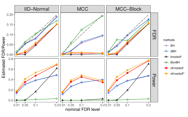
Figure 4: Estimated FDR and TPR under different design matrix settings. cKnockoff/cKnockoff^∗ outperform the other procedures in general.

We observe that cKnockoff controls FDR and dominates knockoff as indicated by our theory. In particular, when knockoff suffers from the threshold phenomenon (small $\alpha$) or the whiteout phenomenon (MCC problem), cKnockoff and cKnockoff^∗ are able to make as many as or even more correct rejections than BH/dBH in average; when knockoff performs well, cKnockoff/cKnockoff^∗ is even better.

The readers might be puzzled by the non-monotone power curve for cKnockoff in the MCC case. This is mainly driven by the shrinking advantage of cKnockoff over knockoffs as $\alpha$ increases. The power gain of cKnockoff over knockoffs is mostly given by the realizations for which $\tau_{1}<\tau$ (i.e., $\mathcal{R}^{\textnormal{Kn}}=\emptyset$) and hence $b_{j}$ is substantially larger than $b_{j}^{0}$. This event happens less likely with a larger $\alpha$. Furthermore, when the signal-to-noise ratio is large to the extent that the ordering of knockoff statistics is relatively stable, only the top $O(1/\alpha)$ variables could gain an extra budget, thus limiting the power boost. This heuristic analysis also suggests that cKnockoff/cKnockoff^∗ only alleviates the whiteout phenomenon to a limited extent because knockoffs, the baseline procedure that cKnockoff wraps around, suffers even when $m_{1}\gg 1/\alpha$. See Appendix F.1.2 for a numerical study. We briefly discuss alternative strategies to handle whiteout in Section 9.

We do not include multiple knockoffs in the comparison here since it requires a larger aspect ratio than $3$. We show the comparison with multiple knockoffs under a different problem setting in Appendix F.1.3. To summarize the results, when $m_{1}<1/\alpha$, multiple knockoffs relieves the threshold phenomenon but underperforms cKnockoff/cKnockoff^∗; when $m_{1}\gg 1/\alpha$, multiple knockoffs is even less powerful than the vanilla knockoffs. Therefore, multiple knockoffs is not as competent as our method in spite of its stronger condition on the sample size.

To see the power improvement of our method over the knockoffs, Figure 5 shows the difference in the TPR of cKnockoff and knockoff at nominal FDR level $\alpha=0.05$ in various design matrices, sparsity, and signal strength settings. The simulation settings are the same as in Section 6.1, with only the number of nonnull variables $m_{1}$ and the signal strength $\beta^{*}$ varying. The superiority of our method is most conspicuous when the problem is sparse and the signal strength is strong. And the power gain is still significant in less preferable settings. Moreover, Theorem 3.3 guarantees that such power gain is always strictly positive, no matter if the problem is sparse, what the design matrix looks like, and how significant the nonnull variables are.

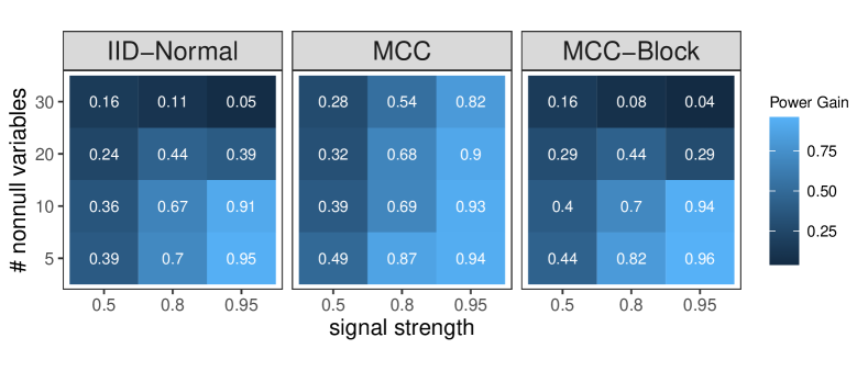
Figure 5: The TPR of cKnockoff minus the TPR of knockoffs in various design matrices, sparsity, and signal strength settings. The three columns each represent a type of design matrix $\boldsymbol{X}$ as described in Section 6.1. The $y$ axis is the number of non-null variables, with a larger value representing a less sparse problem. The $x$ axis represents the TPR of the BH procedure if we run it with nominal FDR level $\alpha=0.2$. A larger value indicates the nonnull variables are more significant.

6.2 Robustness to non-Gaussian noise

In a practical problem, the outcome $\boldsymbol{y}$ may not follow a Gaussian distribution. Here we examine the robustness of our methods to heavy-tailed distributed outcomes. Specifically, the outcome $\boldsymbol{y}$ is generated from $\boldsymbol{y}=\boldsymbol{X}\boldsymbol{\beta}+\boldsymbol{\varepsilon}$, where $\varepsilon_{i}\overset{\textnormal{i.i.d.}}{\sim}t_{k}$ follows the $t$-distribution with degree of freedom $k$. As $k$ decreases, the $t$-distribution gets more heavy-tailed. We set $\alpha=0.2$ and the other simulation settings are the same as in Section 6.1.

Figure 6 shows the FDR of multiple procedures as the noise distribution deviates farther from Gaussian. For all the cases we consider, our methods are robust in the sense that their FDR is still below $\alpha$.

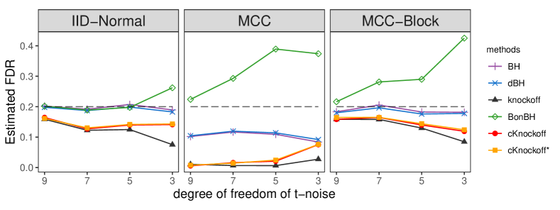
Figure 6: Estimated FDR and TPR when the noise is generated from a heavy-tailed $t$-distribution.

6.3 Scalability

The computation complexity of our methods is instance-specific and the worst-case complexity is uninformative. Nevertheless, we provide a rough analysis of the instance-specific complexity. For every variable that is being examined after the filtering step described in Appendix D, the amount of computation is roughly the same as running a bounded number of rounds of knockoffs with a given knockoff matrix; see Appendix B-D for detail. As a result, if we let $A$ denote the number of variables after filtering, $C_{{\textnormal{Kn}},\mathrm{f}}$ denote the complexity of knockoffs with a given knockoff matrix, and $C_{{\textnormal{Kn}},\mathrm{m}}$ denote the complexity of generating a knockoff matrix, the complexity of our methods is

$$O(A\cdot C_{{\textnormal{Kn}},\mathrm{f}})+C_{{\textnormal{Kn}},\mathrm{m}},$$

because the knockoff matrix is only computed once. By contrast, the complexity of knockoffs is $O(C_{{\textnormal{Kn}},\mathrm{f}})+C_{{\textnormal{Kn}},\mathrm{m}}$. Note that when $A=O(1)$, our method has the same complexity as knockoffs up to a multiplicative constant. In many cases, $A$ is small because our method would only examine a handful of promising variables not rejected by knockoffs. Furthermore, we can force $A$ to be small by exploiting a more stringent filtering step.

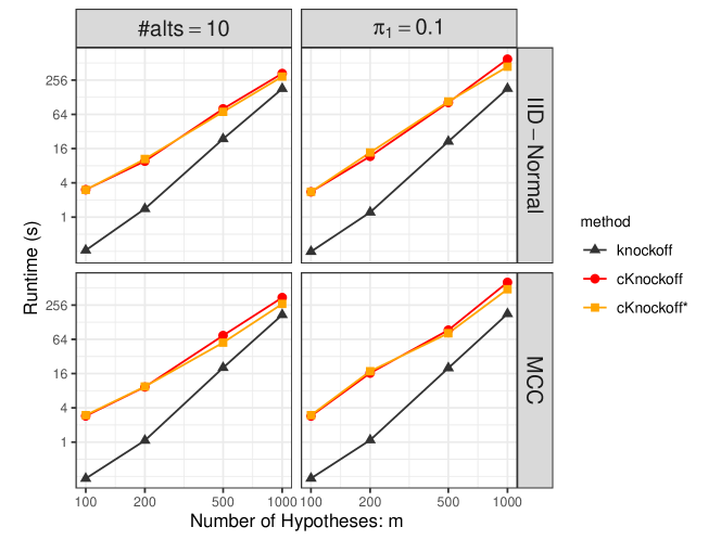
Figure 7: Averaged running time of knockoff, cKnockoff, and cKnockoff^∗ as the problem size increases. The left panel has a fixed number of true alternatives $=10$ as $m$ increases; the right panel has a fixed proportion of true alternatives $=0.1$. All three methods show a roughly $O(m^{3})$ time complexity in the figure.

Figure 7 shows the averaged running time of knockoffs and cKnockoff on a single-core 3.6GHz CPU. In these experiments, we set the signal strength, construct the knockoff matrix, and produce the feature statistics in the same way as in Section 6.1. We set $\alpha=0.05$ and $n=3m$ where $m$ varies from $100$ to $1000$. The left panel of the figure has a fixed number of true alternatives $=10$ as $m$ increases; while the right panel has a fixed proportion of true alternatives $\pi_{1}\coloneqq m_{1}/m=0.1$. As suggested by the heuristic complexity analysis above, the computation time of cKnockoff/cKnockoff^∗ is a small multiple of that of knockoffs in all settings, even with a single core. When multiple cores are available, we can easily parallelize the computation to decide $E_{j}\leq 0$ for different variables or the computation to calculate each $E_{j}$; see our R package for detail.

7 Numerical demonstration of Model-X cKnockoffs

In this section, we demonstrate the model-X cKnockoff procedure on two simple problems, where we set the fallback test statistics naively as $T_{j}=|\boldsymbol{X}_{j}^{\mkern-1.5mu\mathsf{T}}\boldsymbol{y}|$ for illustration purposes. Such $T_{j}$ is usually a poor indicator for whether $H_{j}$ is null or not. A powerful fallback test statistics requires careful considerations based on the specific problem and assumptions, as discussed in Section 5. Therefore, the results in this section are not show-off of the power improvement of the model-X cKnockoff. Instead, they serve as a demonstration of the feasibility and value of our method.

In our simulation setting, the distribution of the covariates $F_{X}$ is mean zero multivariate Gaussian with different types of covariance matrices. Like in Section 6.1, we consider three types of the distribution of the covariates: IID normal, MCC, and MCC-Block, where the covariance matrices are the same as its fixed-X counterpart. For example, the “IID normal” covariates distribution has $F_{X}\sim\mathcal{N}(\boldsymbol{0},\boldsymbol{I}_{p})$ and the “MCC” covariates has $F_{X}\sim\mathcal{N}(\boldsymbol{0},\boldsymbol{\Sigma})$ with

$$\boldsymbol{\Sigma}=\begin{bmatrix}1&-\frac{1}{m}&\ldots&-\frac{1}{m}\\ -\frac{1}{m}&1&\ldots&-\frac{1}{m}\\ \vdots&\vdots&\ddots&\vdots\\ -\frac{1}{m}&-\frac{1}{m}&\ldots&1\\ \end{bmatrix}\in\mathbb{R}^{m\times m}.$$

The other simulation settings are the same as in Section 6.1 if not specified.

7.1 high-dimensional linear regression

In this simulation, we generate the response $y$ via the Gaussian linear model

$$y=\sum_{j=1}^{m}X_{j}\beta_{j}+\varepsilon,\quad\varepsilon\sim\mathcal{N}(0,1)$$

with the number of covariates $m=100$ larger than the number of observations $n=80$. The LCD statistics with $\lambda$ determined by cross-validation are employed as the feature importance statistics.

Figure 8 shows a mild power improvement even when we use the naive fallback test statistics $T_{j}=|\boldsymbol{X}_{j}^{\mkern-1.5mu\mathsf{T}}\boldsymbol{y}|$.

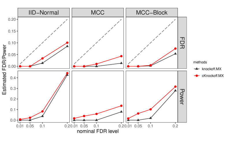
Figure 8: Estimated FDR and TPR under different design matrix settings for model-X knockoffs and cKnockoff in high dimensional linear regression.

7.2 logistic regression

Consider the usual logistic regression setting where we generate $y\in\left\{0,1\right\}$ with

$$\ln\left(\frac{\mathbb{P}(y=1)}{1-\mathbb{P}(y=1)}\right)=\sum_{j=1}^{m}X_{j}\beta_{j}.$$

We have $m=100$ covariates and $n=300$ observations. The feature importance statistics we use is the logistic regression version of the LCD statistics. That is,

$$W_{j}=|\hat{\beta}_{j}|-|\hat{\beta}_{j+m}|,$$

where

$$\hat{\boldsymbol{\beta}}^{\lambda}=\underset{\boldsymbol{\beta}\in\mathbb{R}^{2m}}{\text{argmin}}\;\;\sum_{i=1}^{n}y_{i}\cdot\theta_{i}-\ln\left(e^{\theta_{i}}+1\right)+\lambda\cdot\left\|\boldsymbol{\beta}\right\|_{1},\text{ with }\theta_{i}=\sum_{j=1}^{m}\boldsymbol{X}_{ij}\beta_{j}+\tilde{\boldsymbol{X}}_{ij}\beta_{j+m}$$

is the $L_{1}$ penalized logistic regression coefficients on the augmented covariates $\boldsymbol{X}$ and $\tilde{\boldsymbol{X}}$. The regularity parameter $\lambda$ is determined by cross-validation.

Figure 9 shows, again, a mild power improvement even with the naive fallback test statistics $T_{j}=|\boldsymbol{X}_{j}^{\mkern-1.5mu\mathsf{T}}\boldsymbol{y}|$.

Figure 9: Estimated FDR and TPR under different design matrix settings for model-X knockoffs and cKnockoff in logistic regression.

8 HIV drug resistance data

In this section, we apply the fixed-X cKnockoff and cKnockoff^∗ to detect the mutations in the Human Immunodeficiency Virus (HIV) associated with drug resistance (Rhee et al., 2006), following the analysis in Barber and Candès (2015) and Fithian and Lei (2022).

The dataset includes experimental results on 16 different drugs, each falling into one of three different categories: protease inhibitors (PIs), nucleoside reverse transcriptase inhibitors (NRTIs), and nonnucleoside reverse transcriptase inhibitors (NNRTIs). In each experiment, we have access to a set of genetic mutations and a measure of resistance to each drug for a sample of HIV patients. Following Barber and Candès (2015), we construct a design matrix, without an intercept term, by one-hot encoding the mutation so that $X_{ij}=1$ iff the $j$th mutation is present in the $i$th sample and preprocess the data by discarding mutations that occur fewer than three times and removing duplicated columns. The $16$ drug experiments are of different sizes. Overall, most of them have sample size $n$ between $600$ to $800$ and number of genetic mutations $m$ between $200$ to $300$. Since the ground truth is not available, we evaluate replicability in the same way as Barber and Candès (2015) by comparing the selected mutations to those identified in an independent treatment-selected mutation (TSM) panel of Rhee et al. (2006); see Section 4 of Barber and Candès (2015) for further detail. For each dataset, we will compare BH, knockoffs, cKnockoff, and cKnockoff^∗ described in Section 6.1.

Figure 10 presents the results where we set $\alpha=0.05$. The horizontal dashed line indicates the total number of mutations appearing in the TSM list. So these experiments cover the cases where the number of non-null variables is above, about, or below $1/\alpha$. We see knockoffs suffers in all cases and almost reject nothing. Our cKnockoff and cKnockoff^∗ procedures save knockoffs and make a decent number of discoveries. As a comparison, the BH procedure may not be suitable for these problems since in most experiments the BH discoveries contain more than $\alpha=5\%$ mutations not in the TSM list.

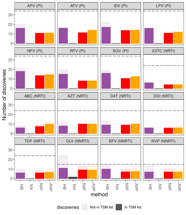
Figure 10: Results on the HIV drug resistance data with $\alpha=0.05$. The darker segments represent the number of discoveries that were replicated in the TSM panel, while the lighter segments represent the number that was not. The horizontal dashed line indicates the total number of mutations appearing in the TSM list. Results are shown for the BH, fixed-$X$ knockoffs, cKnockoff and cKnockoff^∗.

Additional results for $\alpha=0.2$ is included in Appendix G, where knockoffs is not powerless in most problems and our methods are able to make more discoveries.

9 Discussion

9.1 Summary

We have presented a new approach, the calibrated knockoff procedure, for simultaneously testing if the explanatory variables are relevant to the outcome. Our cKnockoff procedure controls FDR and is uniformly more powerful than the knockoff procedure. And the power gain is especially large when the unknown $\boldsymbol{\beta}$ vector is very sparse, in particular when the number of nonzeros in $\boldsymbol{\beta}$ is not much larger than $1/\alpha$. While our new approach is more computationally intensive in principle, we introduce computational tricks that accelerate the method substantially without sacrificing FDR control in theory. Our implementation of cKnockoff turns out to be quite efficient in our numerical experiments in the sense that the computation time is only a small multiple of that of knockoffs, and it can be further accelerated by parallelization.

9.2 Remedies for whiteout

As discussed earlier, cKnockoff only alleviates the whiteout issue (Li and Fithian, 2021) to a limited extent because the signs of knockoff feature statistics are too noisy to be useful for the Selective-Seqstep filter even though the ordering of variables is satisfactory. Meanwhile, BH and dBH are not ideal either because they have bimodal FDP distributions with large masses at around $0$ and $1$. On the other hand, Example 1.1 indicates that the high correlation could help, instead of hurt, inference largely in the presence of sparsity. It would be interesting to investigate the possibility to take advantage of the sparsity which can help inform the ordering of variables without relying on making the sparsity assumption explicitly and resorting to asymptotics.

Reproducibility

Calibrated knockoffs are implemented in an R package available online at the Github repository https://github.com/yixiangLuo/cknockoff. And the R code to reproduce all simulations and figures in this paper can be found at https://github.com/yixiangLuo/cknockoff_expr.

Appendix A Further details on knockoffs

A.1 Deferred proofs

Here, for the sake of completeness, we prove several results that appeared first in Barber and Candès (2015) and other works.

Theorem A.1.

Suppose the feature statistics $\boldsymbol{W}=(W_{1},W_{2},\ldots,W_{m})$ satisfy the sufficiency condition and the anti-symmetry condition. Then

$${\textnormal{sgn}}(W_{j})\,\mid\,|W_{j}|,\,\boldsymbol{W}_{-j}\;\stackrel{{\scriptstyle H_{j}}}{{\sim}}\;\textnormal{Unif}\{-1,+1\}$$

for any $j\in\mathcal{H}_{0}$.

Proof.

It suffices to show for a given arbitrary $j\in[m]$,

$$\boldsymbol{W}\overset{d}{=}(W_{1},\ldots,W_{j-1},-W_{j},W_{j+1},\ldots,W_{m})\triangleq\boldsymbol{W}_{j}^{-}.$$

The sufficiency condition allows us to write

$$\boldsymbol{W}=g(\boldsymbol{X}_{+}^{\mkern-1.5mu\mathsf{T}}\boldsymbol{X}_{+},\boldsymbol{X}_{+}^{\mkern-1.5mu\mathsf{T}}\boldsymbol{y})$$

for some function $g$, where $\boldsymbol{X}_{+}$ is the augmented matrix defined in Section 2.1. The anti-symmetry condition implies

$$\boldsymbol{W}^{-}=g((\boldsymbol{X}^{\text{swap}}_{+})^{\mkern-1.5mu\mathsf{T}}\boldsymbol{X}^{\text{swap}}_{+},(\boldsymbol{X}^{\text{swap}}_{+})^{\mkern-1.5mu\mathsf{T}}\boldsymbol{y}),$$

where $\boldsymbol{X}_{+}^{\text{swap}}$ is obtained by swapping $\boldsymbol{X}_{j}$ and $\tilde{\boldsymbol{X}}_{j}$ in $\boldsymbol{X}_{+}$, i.e.

$$(\boldsymbol{X}^{\text{swap}}_{+})_{j}=(\boldsymbol{X}_{+})_{j+m},\quad(\boldsymbol{X}^{\text{swap}}_{+})_{j+m}=(\boldsymbol{X}_{+})_{j},\quad(\boldsymbol{X}^{\text{swap}}_{+})_{i}=(\boldsymbol{X}_{+})_{i}\;\text{ for }i\neq j,\,j+m.$$

$\boldsymbol{X}_{j}^{\mkern-1.5mu\mathsf{T}}\boldsymbol{X}_{i}=\tilde{\boldsymbol{X}}_{j}^{\mkern-1.5mu\mathsf{T}}\boldsymbol{X}_{i}$ for all $i\neq j$ and $\beta_{j}=0$,

$$(\boldsymbol{X}^{\text{swap}}_{+})^{\mkern-1.5mu\mathsf{T}}\boldsymbol{X}^{\text{swap}}_{+}=\boldsymbol{X}_{+}^{\mkern-1.5mu\mathsf{T}}\boldsymbol{X}_{+},\quad(\boldsymbol{X}^{\text{swap}}_{+})^{\mkern-1.5mu\mathsf{T}}\boldsymbol{X}\beta=\boldsymbol{X}_{+}^{\mkern-1.5mu\mathsf{T}}\boldsymbol{X}\boldsymbol{\beta}$$

Furthermore,

$$(\boldsymbol{X}^{\text{swap}}_{+})^{\mkern-1.5mu\mathsf{T}}\boldsymbol{y}\;\overset{d}{=}\;\mathcal{N}((\boldsymbol{X}^{\text{swap}}_{+})^{\mkern-1.5mu\mathsf{T}}\boldsymbol{X}\boldsymbol{\beta},(\boldsymbol{X}^{\text{swap}}_{+})^{\mkern-1.5mu\mathsf{T}}\boldsymbol{X}^{\text{swap}}_{+})\;\overset{d}{=}\;\mathcal{N}(\boldsymbol{X}_{+}^{\mkern-1.5mu\mathsf{T}}\boldsymbol{X}\boldsymbol{\beta},\boldsymbol{X}_{+}^{\mkern-1.5mu\mathsf{T}}\boldsymbol{X}_{+})\;\overset{d}{=}\;\boldsymbol{X}_{+}^{\mkern-1.5mu\mathsf{T}}\boldsymbol{y}.$$

Therefore,

$$\boldsymbol{W}_{j}^{-}=g((\boldsymbol{X}^{\text{swap}}_{+})^{\mkern-1.5mu\mathsf{T}}\boldsymbol{X}^{\text{swap}}_{+},(\boldsymbol{X}^{\text{swap}}_{+})^{\mkern-1.5mu\mathsf{T}}\boldsymbol{y})\;\overset{d}{=}\;g(\boldsymbol{X}_{+}^{\mkern-1.5mu\mathsf{T}}\boldsymbol{X}_{+},\boldsymbol{X}_{+}^{\mkern-1.5mu\mathsf{T}}\boldsymbol{y})=\boldsymbol{W}.$$

∎

Theorem A.2.

Suppose the feature statistics satisfy the sufficiency condition and the anti-symmetry condition. Then

$$M_{t}\;=\;\frac{|\mathcal{C}(w_{t})\cap\mathcal{H}_{0}|}{1+|\mathcal{A}(w_{t})\cap\mathcal{H}_{0}|}$$

is a supermartingale with respect to the filtration

$$\mathcal{F}_{t}=\sigma\Big{(}\,|W|,\;\left(W_{j}:j\in\mathcal{H}_{0}^{\mathsf{c}}\text{ or }|W_{j}|<w_{t}\right),\;|\mathcal{C}(w_{t})|\,\Big{)}.$$

Moreover, we have $\mathbb{E}[M_{1}]\leq 1$.

Proof.

Without loss of generality, assume $|W_{1}|<\cdots<|W_{m}|$. Then $w_{t}=W_{t}$ and $|W_{j}|<w_{t}$ is equivalent to $j<t$. Let $V^{+}_{t}\coloneqq|\mathcal{C}(w_{t})\cap\mathcal{H}_{0}|$ and $V^{-}_{t}\coloneqq|\mathcal{A}(w_{t})\cap\mathcal{H}_{0}|$ for short. Since the non-null feature statistics are known given $\mathcal{F}_{t}$, it’s easy to see $V^{+}_{t}$ and $V^{-}_{t}$ are measurable with respect to $\mathcal{F}_{t}$. Hence $M_{t}\in\mathcal{F}_{t}$.

To see $\mathcal{F}_{t}$ is indeed a filtration, note $\left\{W_{j}:j\in\mathcal{H}_{0}^{\mathsf{c}}\text{ or }|W_{j}|<w_{t}\right\}$ is monotone in $t$. Given this set and $|\mathcal{C}(w_{t})|$, we are able to compute $|\mathcal{C}(w_{s})|$ for all $s\leq t$. Therefore, $\mathcal{F}_{t}$ is also monotone in $t$, namely, $\mathcal{F}_{t}\subseteq\mathcal{F}_{t+1}$ for all $t$.

It remains to show $\mathbb{E}[M_{t+1}\mid\mathcal{F}_{t}]\leq M_{t}$. By construction, $M_{t+1}=M_{t}$ if $t\in\mathcal{H}_{0}^{\mathsf{c}}$. Otherwise

$$M_{t+1}=\frac{V^{+}_{t}-\mathbf{1}\left\{W_{t}>0\right\}}{1+V^{-}_{t}-(1-\mathbf{1}\left\{W_{t}>0\right\})}=\frac{V^{+}_{t}-\mathbf{1}\left\{W_{t}>0\right\}}{(V^{-}_{t}+\mathbf{1}\left\{W_{t}>0\right\})\vee 1}.$$

Theorem A.1 implies that

$${\textnormal{sgn}}(W_{j})\,\mid\,|\boldsymbol{W}|,\,\left(W_{i}:i\in\mathcal{H}_{0}^{\mathsf{c}}\text{ or }i<t\right)\overset{\textnormal{i.i.d.}}{\sim}\textnormal{Unif}\{-1,+1\},\quad\text{for }j\in\mathcal{H}_{0}\text{ and }j\geq t.$$

Hence

$$\mathbb{P}(W_{t}>0\mid\mathcal{F}_{t})=\frac{V^{+}_{t}}{V^{+}_{t}+V^{-}_{t}}.$$

Therefore

$$\mathbb{E}[M_{t+1}\mid\mathcal{F}_{t}]\;=\;\frac{1}{V^{+}_{t}+V^{-}_{t}}\left[V^{+}_{t}\frac{V^{+}_{t}-1}{V^{-}_{t}+1}+V^{-}_{t}\frac{V^{+}_{t}}{V^{-}_{t}\vee 1}\right]\;=\;\begin{cases}\frac{V^{+}_{t}}{1+V^{-}_{t}}=M_{t},&V^{-}_{t}>0\\ V^{+}_{t}-1=M_{t}-1,&V^{-}_{t}=0\end{cases}.$$

So $M_{t}$ is s supermartingale with respect to the filtration $\mathcal{F}_{t}$.

To show $\mathbb{E}[M_{1}]\leq 1$, note that $V^{+}_{1}\mid|\boldsymbol{W}|\sim\text{Binomial}(m_{0},1/2)$. We have

$$\mathbb{E}\left[M_{1}\mid|\boldsymbol{W}|\right] \;=\;\mathbb{E}\left[\frac{V^{+}_{1}}{1+m_{0}-V^{+}_{1}}\mid|\boldsymbol{W}|\right]\;=\;\sum_{i=1}^{m_{0}}\mathbb{P}(V^{+}_{1}=i)\cdot\frac{i}{1+m_{0}-i}$$

$$\;=\;\sum_{i=1}^{m_{0}}\frac{1}{2^{m_{0}}}\frac{m_{0}!}{i!(m_{0}-i)!}\cdot\frac{i}{1+m_{0}-i}\;=\;\sum_{i=1}^{m_{0}}\frac{1}{2^{m_{0}}}\frac{m_{0}!}{(i-1)!(m_{0}-i+1)!}$$

$$\;=\;\sum_{i=1}^{m_{0}}\mathbb{P}(V^{+}_{1}=i-1)\leq 1.$$

Then $\mathbb{E}[M_{1}]=\mathbb{E}\left[\mathbb{E}\left[M_{1}\mid|\boldsymbol{W}|\right]\right]\leq 1$. ∎

A.2 A faster version of the LSM statistic

The LSM statistic defined in (5) is computationally burdensome because it requires calculating the entire lasso path. Even if the great majority of variables are null, they will eventually enter and leave the model in a chaotic process once $\lambda$ becomes small enough. If we stop too early, most variables will never enter, so their feature statistics will be zero and there will be no chance to discover them, but if we stop too late, we will consume most of our computational resources fitting null variables at the end of the path. In practice, the path is also calculated only for a fine grid of $\lambda$ values, which has the added undesirable effect of introducing artificial ties between variables.

This section introduces a more computationally efficient alternative that uses a coarser grid of $\lambda$ values and also stops the path early, but breaks ties by using variables’ correlations using the residuals at each stage. Assume we calculate the lasso fit $\hat{\boldsymbol{\beta}}^{\lambda(\ell)}$ for $\ell=0,\ldots,L$ on a coarse grid defined by:

$$\max_{1\leq j\leq 2m}\lambda_{j}^{*}=\lambda_{\text{max}}=\lambda(0)>\lambda(1)>\cdots>\lambda(L)=\lambda_{\text{min}}=2\tilde{\sigma}\wedge\frac{\lambda_{\text{max}}}{2}.$$

We stop the path at $2\tilde{\sigma}$ because we find it tends to set most null variables’ coefficients to zero, we take $\lambda(0),\ldots,\lambda(L)$ to be a decreasing geometric sequence:

$$\lambda(\ell)=\lambda(0)\cdot\zeta^{\ell},\quad\text{ for }\zeta=\left(\frac{\lambda(L)}{\lambda(0)}\right)^{1/L}.$$

Then for variable $j=1,\ldots,2m$, define its (discrete) time of entry as

$$\ell_{j}^{*}=\min\left\{\ell\in\{1,\ldots,L\}:\;\hat{\beta}_{j}^{\lambda(\ell)}\neq 0\right\},$$

with $\ell_{j}^{*}=L+1$ if the set is empty. To break ties between these discrete values, we use each variable’s correlation with the lasso residuals at $\lambda_{j}^{+}=\lambda(\ell_{j}^{*}-1)$, the last fit in the discrete path before variable $j$ enters:

$$\rho_{j}=\left|(\boldsymbol{X}_{+})_{j}^{\mkern-1.5mu\mathsf{T}}\boldsymbol{r}^{\lambda_{j}^{+}}\right|\leq\lambda_{j}^{+},\quad\text{ where }\boldsymbol{r}^{\lambda}=\boldsymbol{y}-\boldsymbol{X}_{+}\hat{\boldsymbol{\beta}}^{\lambda}.$$

$\rho_{j}$ can be considered an estimate of $\lambda_{j}^{*}$, since we have

$$\lambda_{j}^{*}=\left|(\boldsymbol{X}_{+})_{j}^{\mkern-1.5mu\mathsf{T}}r^{\lambda_{j}^{*}}\right|\approx\left|(\boldsymbol{X}_{+})_{j}^{\mkern-1.5mu\mathsf{T}}r^{\lambda_{j}^{+}}\right|.$$

To combine these, we can use any transform that orders variables first by $\lambda_{j}^{+}$ and then by $\rho_{j}$. We use a transform that also aids the accuracy of the local linear regression approximation of $W_{j}(\boldsymbol{z})$ on $\boldsymbol{X}_{j}^{\mkern-1.5mu\mathsf{T}}\boldsymbol{z}$. Let $\iota$ denote a small positive quantity and $\lambda(L+1)=0$, and define

$$\hat{\lambda}_{j}\;=\;\max\{\rho_{j}-\iota,\;\lambda(\ell_{j}^{*})\}+\iota\rho_{j}/\lambda_{j}^{+}\;\approx\;\max\{\rho_{j},\,\lambda(\ell_{j}^{*})\}.$$

Finally, we define the coarse LSM (C-LSM) feature statistics by substituting $\hat{\lambda}_{j}$ for $\lambda_{j}^{*}$ in (5):

$$W_{j}^{\text{C-LSM}}=(\hat{\lambda}_{j}\vee\hat{\lambda}_{j+m})\cdot{\textnormal{sgn}}(\hat{\lambda}_{j}-\hat{\lambda}_{j+m}).$$

A.3 numerical comparisons

Here we compare the performance of the vanilla LSM feature statistics with our LCD-T and C-LSM. Figure 11 has settings the same as in Section 6.1 and Figure 12 is less sparse with $m_{1}=50$ while using a different $\lambda=\tilde{\sigma}$. We see the performance of C-LSM is roughly the same as the original LSM in all cases we consider and LCD-T is sometimes even better, as suggested in Weinstein et al. (2020).

Figure 11: Estimated FDR and TPR of knockoffs employing LSM, LCD-T or C-LSM as feature statistics, where $m_{1}=10$ and $\lambda=2\tilde{\sigma}$ in LCD-T.

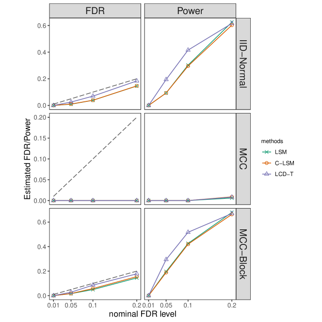
Figure 12: Estimated FDR and TPR of knockoffs employing LSM, LCD-T or C-LSM as feature statistics, where $m_{1}=50$ and $\lambda=\tilde{\sigma}$ in LCD-T.

Appendix B Implementation: calculations to check if $\tilde{E}_{j}\leq 0$

In this section we continue Section 4, regarding $S_{j}(\boldsymbol{y})$, $c=T_{j}(\boldsymbol{y})$, and $Q_{j}(\cdot\mid S_{j}(\boldsymbol{y}))$ as fixed and use $\boldsymbol{z}$ to denote a generic response vector drawn from the conditional null distribution $Q_{j}$. We will explain the sampling scheme, the construction of $\widetilde{\Omega}_{j}$, and the way to control numerical error when checking if $\tilde{E}_{j}\leq 0$.

B.1 Sampling $\boldsymbol{y}$ conditional on $S_{j}(\boldsymbol{y})$ under $H_{j}$

We first fix a basis to make our calculations convenient. Let $\boldsymbol{V}_{-j}\in\mathbb{R}^{n\times(m-1)}$ denote an orthonormal basis for the column span of $\boldsymbol{X}_{-j}$, so that $\boldsymbol{\Pi}_{-j}=\boldsymbol{V}_{-j}\boldsymbol{V}_{-j}^{\mkern-1.5mu\mathsf{T}}$. Next, for the projection of $\boldsymbol{X}_{j}$ orthogonal to the span of $\boldsymbol{X}_{-j}$, define the unit vector in that direction:

$$\boldsymbol{v}_{j}=\frac{\boldsymbol{\Pi}_{-j}^{\perp}\boldsymbol{X}_{j}}{\|\boldsymbol{\Pi}_{-j}^{\perp}\boldsymbol{X}_{j}\|},\quad\text{ where }\boldsymbol{\Pi}_{-j}^{\perp}=\boldsymbol{I}-\boldsymbol{\Pi}_{-j}$$

Finally, let $\boldsymbol{V}_{\text{res}}\in\mathbb{R}^{n\times(n-m)}$ denote an orthonormal basis for the subspace orthogonal to the span of $\boldsymbol{X}$. Then we can decompose $\boldsymbol{z}$ as

$$\boldsymbol{z}=\boldsymbol{V}_{-j}\boldsymbol{V}_{-j}^{\mkern-1.5mu\mathsf{T}}\boldsymbol{z}+\boldsymbol{v}_{j}\cdot\eta+\boldsymbol{V}_{\text{res}}\cdot\boldsymbol{r},$$

where $\eta=\boldsymbol{v}_{j}^{\mkern-1.5mu\mathsf{T}}\boldsymbol{z}\in\mathbb{R}$ is the component of $\boldsymbol{z}$ in the direction $\boldsymbol{v}_{j}$, and $\boldsymbol{r}=\boldsymbol{V}_{\text{res}}^{\mkern-1.5mu\mathsf{T}}\boldsymbol{z}\in\mathbb{R}^{n-m}$ is the residual component.

Recall that $Q_{j}$ is uniform on its support $\{\boldsymbol{z}:\;S_{j}(\boldsymbol{z})=S_{j}(\boldsymbol{y})\}$ (see Appendix E.2). Fixing $S_{j}(\boldsymbol{z})=S_{j}(\boldsymbol{y})$ is equivalent to constraining

$$\boldsymbol{V}_{-j}^{\mkern-1.5mu\mathsf{T}}\boldsymbol{z}=\boldsymbol{V}_{-j}^{\mkern-1.5mu\mathsf{T}}\boldsymbol{y},\quad\text{ and }\;\eta^{2}+\|\boldsymbol{r}\|^{2}=\|\boldsymbol{\Pi}_{-j}^{\perp}\boldsymbol{z}\|^{2}=\|\boldsymbol{\Pi}_{-j}^{\perp}\boldsymbol{y}\|^{2}.$$

Let $\rho^{2}=\|\boldsymbol{\Pi}_{-j}^{\perp}\boldsymbol{y}\|^{2}$, which depends only on $S_{j}(\boldsymbol{y})$. We can sample $\boldsymbol{z}\sim Q_{j}$ by first sampling

$$(\eta,\boldsymbol{r})\sim\text{Unif}\left(\rho\cdot\mathbb{S}^{n-m}\right),$$

where $\mathbb{S}^{n-m}\subseteq\mathbb{R}^{n-m+1}$ is the unit sphere of dimension $n-m$, and then reconstructing $\boldsymbol{z}$ using equation (31).

To sample from $\widetilde{\Omega}_{j}$, we add a further constraint on $\eta$, that it lies in some union of intervals $U_{j}\subseteq[-\rho,\rho]$. See Appendix B.2 for details. In order to sample $\boldsymbol{z}$ satisfying this constraint efficiently, we first sample $\eta$ marginally obeying the constraint and then $\boldsymbol{r}$ conditional on $\eta$. Standard calculations show the cumulative distribution function (CDF) of $\eta$ is

$$F_{\eta}(x;S_{j})\coloneqq\mathbb{P}(\eta\leq x)=F_{t_{n-m}}\left(\frac{x\sqrt{n-m}}{\sqrt{(\rho^{2}-x^{2})}}\right)\;\;\text{for }|x|<\rho,$$ (30)

where $F_{t_{n-m}}$ is the CDF of the t-distribution with degree of freedom $n-m$. Now write $\boldsymbol{r}=\|\boldsymbol{r}\|\cdot\boldsymbol{u}$ with $\boldsymbol{u}$ being the direction of $\boldsymbol{r}$. Given $\eta$, we have $\|\boldsymbol{r}\|=\sqrt{\rho^{2}-\eta^{2}}$ and $\boldsymbol{u}\sim\text{Unif}(\mathbb{S}^{n-m-1})$ is independent of $\eta$.

To conclude, we sample $\eta\sim F_{\eta}$ in the desired union of intervals and $\boldsymbol{u}\sim\text{Unif}(\mathbb{S}^{n-m-1})$ independently. The $\boldsymbol{z}$ is given by

$$\boldsymbol{z}(\eta,\boldsymbol{u})=\boldsymbol{V}_{-j}\boldsymbol{V}_{-j}^{\mkern-1.5mu\mathsf{T}}\boldsymbol{y}+\boldsymbol{v}_{j}\cdot\eta+\sqrt{\rho^{2}-\eta^{2}}\cdot\boldsymbol{V}_{\text{res}}\boldsymbol{u}.$$ (31)

B.2 The construction of $\widetilde{\Omega}_{j}$

Section 4 describes $\widetilde{\Omega}_{j}$ in terms of $\boldsymbol{X}_{j}^{\mkern-1.5mu\mathsf{T}}\boldsymbol{z}$. To be consistent with the sampling scheme, we first rephrase $\widetilde{\Omega}_{j}$ in terms of $\eta$ as used in (31).

We decompose

$$\boldsymbol{X}_{j}^{T}\boldsymbol{z}=\boldsymbol{X}_{j}^{T}\boldsymbol{\Pi}_{-j}\boldsymbol{z}+(\boldsymbol{v}_{j}^{\mkern-1.5mu\mathsf{T}}\boldsymbol{X}_{j})\cdot\eta,$$ (32)

which establishes a linear relationship between $\boldsymbol{X}_{j}^{\mkern-1.5mu\mathsf{T}}\boldsymbol{z}$ and $\eta$ (recall $\boldsymbol{\Pi}_{-j}\boldsymbol{z}=\boldsymbol{\Pi}_{-j}\boldsymbol{y}$ is fixed). Thus we can write

$$\widetilde{\Omega}_{j}\;=\;\{\boldsymbol{z}(\eta,\boldsymbol{u})\in\textnormal{Supp}(Q_{j}):\;\eta\in A_{j}\},\quad\text{ for }A_{j}=A_{j}^{-}\cup(a_{j}^{(1)},a_{j}^{(2)})^{\mathsf{c}},$$

where $a_{j}^{(1)}$ and $a_{j}^{(2)}$ are solved from

$$\{\boldsymbol{z}(\eta,\boldsymbol{u})\in\textnormal{Supp}(Q_{j}):\;\eta\in(a_{j}^{(1)},a_{j}^{(2)})^{\mathsf{c}}\}\;=\;\Omega_{j}^{+}(\boldsymbol{y})\;=\;\{\boldsymbol{z}\in\textnormal{Supp}(Q_{j}):\;T_{j}(\boldsymbol{z})\geq c\}$$ (33)

and $A_{j}^{-}$ is a union of intervals in order to have

$$\{\boldsymbol{z}(\eta,\boldsymbol{u})\in\textnormal{Supp}(Q_{j}):\;\eta\in A_{j}^{-}\}\approx\Omega_{j}^{-}(\boldsymbol{y}).$$

Note we reuse the notation $A_{j}$, $A_{j}^{-}$, $a_{j}^{(1)}$, and $a_{j}^{(2)}$ as the constraint sets or boundaries for $\eta$ and they should not be confused with those in Section 4.

In the rest of this section, we give explicit ways to obtain $a_{j}^{(1)}$, $a_{j}^{(2)}$, and $A_{j}^{-}$.

For $a_{j}^{(1)}$ and $a_{j}^{(2)}$, note

$$\Omega_{j}^{+}(\boldsymbol{y})\;=\;\left\{\boldsymbol{z}\in\textnormal{Supp}(Q_{j}):\;\left|\boldsymbol{X}_{j}^{\mkern-1.5mu\mathsf{T}}\left(\boldsymbol{z}-\hat{\boldsymbol{y}}^{(j)}(S_{j})\right)\right|\geq c\right\}.$$

Using (32), direct calculation shows

$$a_{j}^{(1)}=\frac{\hat{\boldsymbol{y}}^{(j)}(S_{j})-\boldsymbol{X}_{j}^{\mkern-1.5mu\mathsf{T}}\boldsymbol{\Pi}_{-j}\boldsymbol{y}-c}{\boldsymbol{v}_{j}^{\mkern-1.5mu\mathsf{T}}\boldsymbol{X}_{j}},\quad a_{j}^{(2)}=\frac{\hat{\boldsymbol{y}}^{(j)}(S_{j})-\boldsymbol{X}_{j}^{\mkern-1.5mu\mathsf{T}}\boldsymbol{\Pi}_{-j}\boldsymbol{y}+c}{\boldsymbol{v}_{j}^{\mkern-1.5mu\mathsf{T}}\boldsymbol{X}_{j}}.$$

For $A_{j}^{-}$, note

$$\Omega_{j}^{-}=\left\{\boldsymbol{z}\in\textnormal{Supp}(Q_{j}):\;j\in\mathcal{C}(w_{\tau_{1}})\right\}\;\subseteq\;\left\{\boldsymbol{z}\in\textnormal{Supp}(Q_{j}):\;|W_{j}|\geq w_{\tau_{1}}\right\}.$$

Hence we want to set $\widetilde{\Omega}_{j}$ as $\left\{\boldsymbol{z}\in\textnormal{Supp}(Q_{j}):\;|W_{j}|\geq w_{\tau_{1}}\right\}$, which is approximately identified by local linear regression.

Specifically, we treat $\boldsymbol{z}=\boldsymbol{z}(\eta,\boldsymbol{u})$ as a one-dimensional random function of $\eta$ with $\boldsymbol{u}$ being an independent random noise. Our local linear regression scheme then regresses $|W_{j}|$ and $w_{\tau_{1}}$ on $\eta$, and solve for the region where $|W_{j}|\geq w_{\tau_{1}}$ numerically.

Our method is motivated by the following observations in simulation studies.

1. Given a fixed $\boldsymbol{u}$, for the lasso-based LSM (C-LSM) and LCD (LCD-T) feature statistics we consider, $|W_{j}(\boldsymbol{z})|$ is roughly a piecewise linear function of $\eta$;

2. $|W_{j}|\approx\mathbb{E}\left[|W_{j}|\mid\eta\right]$, or say, the noise caused by $\boldsymbol{u}$ is small, if $\mathbb{E}\left[|W_{j}|\mid\eta\right]$ is large. Specifically, we observe that the standard deviation of $|W_{j}|$ conditional on $\eta$ is typically a small fraction of the conditional mean when $\mathbb{E}\left[|W_{j}|\mid\eta\right]\geq\mathbb{E}\left[w_{\tau_{1}}\mid\eta\right]$.

Heuristically, the first observation is because that the KKT conditions of Lasso is a piecewise linear system. And the second is that the randomness in $\boldsymbol{u}$ contributes to the correlation between $\boldsymbol{y}$ and the knockoff variables, which is considered noise. When $|W_{j}|$ is large, such a noise is expected to be dominated by the signal from the original variable. $w_{\tau_{1}}$ shares a similar behavior, though its value is determined by a more complicated mechanism.

We then approximate

$$\left\{\boldsymbol{z}\in\textnormal{Supp}(Q_{j}):\;|W_{j}|\geq w_{\tau_{1}}\right\}\approx\left\{\boldsymbol{z}\in\textnormal{Supp}(Q_{j}):\,\mathbb{E}\left[|W_{j}|\mid\eta\right]\geq\mathbb{E}\left[w_{\tau_{1}}\mid\eta\right]\right\},$$

with the conditional expectation estimated by the local linear regression.

To be specific, the construction of $\widetilde{\Omega}_{j}^{-}$ is done as follows.

1. sample $\boldsymbol{z}_{1}(\eta_{1},u_{1}),\ldots,\boldsymbol{z}_{k}(\eta_{k},u_{k})$ such that $\eta_{1},\ldots,\eta_{k}$ are equi-spaced nodes in $[-\rho,\rho]$ and $u_{1},\ldots,u_{k}$ are independent drawn from $\text{Unif}(\mathbb{S}^{n-m-1})$.

2. compute $|W_{j}(\boldsymbol{z}_{i})|$ and $w_{\tau_{1}}(\boldsymbol{z}_{i})$ for each $i$.

3. estimate $\mathbb{E}[|W_{j}(\boldsymbol{z})|\mid\eta]$, denoted as $\widehat{W}_{j}(\eta)$, by a local linear regression on $|W_{j}(\boldsymbol{z}_{i})|$ for $i=1,\ldots,k$. We use the Gaussian kernel and set the bandwidth as the distance between consecutive nodes $\eta_{i}-\eta_{i-1}$. Similarly, estimate $\mathbb{E}[w_{\tau_{1}}(\boldsymbol{z})\mid\eta]$ as $\widehat{w}(\eta)$.

4. $\widetilde{\Omega}_{j}^{-}$ is then

   $$\widetilde{\Omega}_{j}^{-}\;=\;\{\boldsymbol{z}\in\textnormal{Supp}(Q_{j}):\;\eta\in A_{j}^{-}\},\quad A_{j}^{-}\coloneqq\left\{\eta:\widehat{W}_{j}(\eta)\geq\widehat{w}(\eta)\right\},$$

   where the inequality $\widehat{W}_{j}(\eta)\geq\widehat{w}(\eta)$ is solved numerically.

B.3 Numerical error control

With enough computational budget, we can compute $\widetilde{E}_{j}$ at arbitrary precision. While in practice, we should tolerate some level of numerical error introduced by Monte-Carlo. The key idea for such error control is to upper bound the probability of mistakenly claiming the sign of $\widetilde{E}_{j}$ at some $\alpha_{c}$.

Our process of deciding ${\textnormal{sgn}}(\widetilde{E}_{j})$ can be formalized as constructing a confidence interval for $\widetilde{E}_{j}$ from a sequence of i.i.d. samples $f_{j}(\boldsymbol{z}_{1}),\,f_{j}(\boldsymbol{z}_{2}),\,\ldots,f_{j}(\boldsymbol{z}_{k})$, with a common mean $\widetilde{E}_{j}/Q_{j}(\widetilde{\Omega}_{j})$. For each $k=1,\,2,\,\ldots$, such a confidence interval at level $\alpha_{c}$, $C_{k}(f_{j}(\boldsymbol{z}_{1}),\,\ldots,f_{j}(\boldsymbol{z}_{k});\,\alpha_{c})$, is computed and once we see it excludes $0$, we stop the calculation and decide if $\widetilde{E}_{j}\leq 0$ accordingly.

To control the sign error for $\widetilde{E}_{j}$, it suffices to have the sequence of confidence intervals $C_{k}$ hold for all (infinite many) $k$ simultaneously,

$$\mathbb{P}(\exists k:\,\widetilde{E}_{j}\not\in C_{k}(f_{j}(\boldsymbol{z}_{1}),\,\ldots,f_{j}(\boldsymbol{z}_{k}))\leq\alpha_{c}.$$

We can further control the inflation of the FDR due to the Monte-Carlo error, as shown next.

Proposition B.1.

Let $\alpha_{c}(\boldsymbol{y})=\mathcal{R}^{{\textnormal{Kn}}(\alpha)}(\boldsymbol{y})\cdot\alpha_{0}/m$ for some constant $\alpha_{0}$ and reject

$$\mathcal{R}=\mathcal{R}^{{\textnormal{Kn}}(\alpha)}\cup\left\{j:\;\exists k,\;\text{s.t. }x\leq 0\text{ for all }x\in C_{k}(f_{j}(\boldsymbol{z}_{1}),\,\ldots,f_{j}(\boldsymbol{z}_{k});\,\alpha_{c})\right\}.$$

Note $\mathcal{R}$ is the cKnockoff rejection set if we compute $E_{j}$ and claim its sign with confidence as described above. Then

$$\textnormal{FDR}(\mathcal{R})\leq\alpha+\alpha_{0}.$$

Proof.

Denote event $D_{j}\coloneqq\left\{\exists k,\;\text{s.t. }x\leq 0\text{ for all }x\in C_{k}(f_{j}(\boldsymbol{z}_{1}),\,\ldots,f_{j}(\boldsymbol{z}_{k});\,\alpha_{c})\right\}$ and

$$D_{j}^{\text{in}}\coloneqq D\cap\left\{\forall k,\;\widetilde{E}_{j}\in C_{k}\right\},\quad D_{j}^{\text{out}}\coloneqq D\cap\left\{\exists k,\;\widetilde{E}_{j}\not\in C_{k}\right\}.$$

Recall $D_{j}^{\text{in}}$ implies $T_{j}\geq\hat{c}_{j}$. And we have $\mathbb{P}(D_{j}^{\text{out}}\mid\boldsymbol{y})\leq\alpha_{c}$ by the construction of $C_{k}$. Therefore, we have

$$\mathbb{E}_{H_{j}}[\textnormal{DP}_{j}(\mathcal{R})\mid S_{j}] \;=\;\mathbb{E}_{H_{j}}\left[\frac{\mathbf{1}\left\{j\in\mathcal{R}^{\textnormal{Kn}}\right\}\vee\mathbf{1}\left\{D_{j}\right\}}{\left|\mathcal{R}\cup\{j\}\right|}\;\Big{|}\;S_{j}\right]$$

$$\;\leq\;\mathbb{E}_{H_{j}}\left[\frac{\mathbf{1}\left\{j\in\mathcal{R}^{\textnormal{Kn}}\right\}\vee\mathbf{1}\left\{T_{j}\geq\hat{c}_{j}\right\}\vee\mathbf{1}\left\{D_{j}^{\text{out}}\right\}}{\left|\mathcal{R}^{\textnormal{Kn}}\cup\{j\}\right|}\;\Big{|}\;S_{j}\right]$$

$$\;\leq\;\mathbb{E}_{H_{j}}[b_{j}\mid S_{j}]+\mathbb{E}_{H_{j}}\left[\frac{\mathbf{1}\left\{D_{j}^{\text{out}}\right\}}{\left|\mathcal{R}^{\textnormal{Kn}}\cup\{j\}\right|}\;\Big{|}\;S_{j}\right].$$

Marginalizing over $S_{j}$, we have

$$\textnormal{FDR}(\mathcal{R})=\sum_{j\in\mathcal{H}_{0}}\mathbb{E}[\,\textnormal{DP}_{j}(\mathcal{R})\,]\leq\sum_{j\in\mathcal{H}_{0}}\mathbb{E}[b_{j}]+\sum_{j\in\mathcal{H}_{0}}\mathbb{E}\left[\mathbb{E}\left[\frac{\mathbf{1}\left\{D_{j}^{\text{out}}\right\}}{\left|\mathcal{R}^{\textnormal{Kn}}(\boldsymbol{y})\cup\{j\}\right|}\;\Big{|}\;\boldsymbol{y}\right]\right]\leq\alpha+\alpha_{0}.$$

∎

Remark B.1.

The denominator $m$ in our choice of $\alpha_{c}$ can be replaced by the number of hypotheses that survived after filtering (see Appendix C), which would increase $\alpha_{c}$ and save some computation time while keeping the same FDR control.

Remark B.2.

In practice, the above bound is rather loose and we found the FDR inflation is ignorable in most cases. In our implementation, we truncate the Monte-Carlo sample sequence and use their sample mean to decide if $\widetilde{E}_{j}\leq 0$ once we already have $500$ samples but still $0\in C_{k}$ for all $k=1,\ldots,500$.

In particular, since the values of $f_{j}(z_{k})$ are bounded, we apply Theorem 3 in Waudby-Smith and Ramdas (2020) to construct such a confidence sequence $C_{k}$, which is adaptive to the sample variance and achieves state-of-the-art performance for bounded random variables.

Appendix C Implementation: filtering the rejection set beforehand

As suggested by Theorem 3.2, we reject the filtered cKnockoff rejection set

$$\mathcal{R}=\mathcal{R}^{{\textnormal{Kn}}}\cup\{j\in\mathcal{S}:\;E_{j}(T_{j};S_{j})\leq 0\}\;\subseteq\;\mathcal{R}^{\textnormal{cKn}}$$

for some set $\mathcal{S}$ that only contains the hypotheses likely to be rejected by cKnockoff. In practice, we find it is a good choice to set

$$\mathcal{S}(s;\boldsymbol{y})=(\mathcal{S}^{\textnormal{BH}}(s;\boldsymbol{y})\cap\mathcal{S}^{\text{p}}(s;\boldsymbol{y}))\cup\mathcal{S}^{{\textnormal{Kn}}}(s;\boldsymbol{y})\setminus\mathcal{R}^{\textnormal{Kn}}(\boldsymbol{y}),$$ (34)

where

$$\mathcal{S}^{\textnormal{BH}}=\mathcal{R}^{{\textnormal{BH}}(s\cdot 4\alpha)},\quad\mathcal{S}^{\text{p}}=\left\{j:\;p_{j}\leq s\cdot\alpha/2\right\},\quad\mathcal{S}^{{\textnormal{Kn}}}=\left\{j:\;|W_{j}|\geq w_{m-|\mathcal{S}^{\textnormal{BH}}\cap\mathcal{S}^{\text{p}}|}\wedge w_{\tau}\right\}$$

with $s=1$. In words, $\mathcal{S}^{\textnormal{BH}}\cap\mathcal{S}^{\text{p}}$ requires that any $j\in\mathcal{S}$ to have a relatively small $p$-value and $\mathcal{S}^{{\textnormal{Kn}}}$ requires $|W_{j}|$ to be relatively large. By the construction of the fallback test, $H_{j}$ is very unlikely to be rejected by cKnockoff if it has a large $p$-value and a small $|W_{j}|$. Among our simulations, this choice almost does not exclude any rejections in the vanilla cKnockoff and achieves $|S|\ll m$. That is to say, it preserves the power of cKnockoff when accelerating it a lot by filtering out many non-promising hypotheses.

Moreover, such filtering can be done in an online manner. Let

$$s^{+}_{j}(\boldsymbol{y})=\min\left\{s:\;j\in\mathcal{S}(s;\boldsymbol{y})\right\}.$$ (35)

Then $s^{+}_{j}$, which we call promising score, roughly measures how likely $H_{j}$ will be rejected by cKnockoff. Then we can check $E_{j}(T_{j};S_{j})\leq 0$ sequentially on the hypotheses ranked by their promising scores. Theorem 3.2 allows us to stop at any time we like and report the rejection set with a valid FDR control. This feature is available in our R package but not employed in the numerical experiments shown in this paper.

To apply filtering to cKnockoff^∗, we reject the filtered cKnockoff^∗ rejection set

$$\mathcal{R}=\mathcal{R}^{{\textnormal{Kn}}}\cup\{j\in\mathcal{S}:\;E^{*}_{j}(T_{j};S_{j})\leq 0\}\;\subseteq\;\mathcal{R}^{{\textnormal{cKn}}^{*}}$$

where $\mathcal{S}$ is further required to satisfy $\mathcal{R}^{\textnormal{Kn}}\cup\mathcal{S}\supseteq\mathcal{R}^{*}$. Like in cKnockoff, Theorem C.1 shows such filtering does not hurt the FDR control.

Theorem C.1.

For any rejection rule $\mathcal{R}$ with $\mathcal{R}^{*}\subseteq\mathcal{R}\subseteq\mathcal{R}^{{\textnormal{cKn}}^{*}}$ almost surely, we have $\textnormal{FDR}(\mathcal{R})\leq\alpha$.

Proof.

Recall

$$\mathcal{R}^{{\textnormal{cKn}}^{*}}\,=\,\mathcal{R}^{{\textnormal{Kn}}}\cup\{j:\;T_{j}\geq\hat{c}_{j}^{*}\}.$$

Hence $\mathcal{R}^{*}\subseteq\mathcal{R}\subseteq\mathcal{R}^{{\textnormal{cKn}}^{*}}$ implies

$$\mathbb{E}_{H_{j}}[\textnormal{DP}_{j}(\mathcal{R})\mid S_{j}]\;\leq\;\mathbb{E}_{H_{j}}\left[\frac{\mathbf{1}\left\{j\in\mathcal{R}^{\textnormal{Kn}}\right\}\vee\mathbf{1}\left\{T_{j}\geq\hat{c}_{j}^{*}\right\}}{\left|\mathcal{R}^{*}\cup\{j\}\right|}\;\Big{|}\;S_{j}\right]\\ \;\leq\;\mathbb{E}_{H_{j}}[b_{j}\mid S_{j}],$$

so that $\textnormal{FDR}(\mathcal{R})\leq\sum_{j\in\mathcal{H}_{0}}\mathbb{E}[b_{j}]\leq\alpha$. ∎

For cKnockoff^∗, $\mathcal{S}$ is set again by (34). The condition $\mathcal{R}^{\textnormal{Kn}}\cup\mathcal{S}\supseteq\mathcal{R}^{*}$ is made true by the construction of $\mathcal{R}^{*}$ in Appendix D.

Appendix D Refined cKnockoff procedure

D.1 Refined cKnockoff procedure

Recall in the refined calibrated knockoff (cKnockoff^∗) procedure, we find certain $\mathcal{R}^{*}$ satisfying $\mathcal{R}^{\textnormal{Kn}}\subseteq\mathcal{R}^{*}\subseteq\mathcal{R}^{\textnormal{cKn}}$. Then cKnockoff^∗ rejects

$$\mathcal{R}^{{\textnormal{cKn}}^{*}}\;=\;\mathcal{R}^{\textnormal{Kn}}\cup\left\{j:\;T_{j}\geq\hat{c}_{j}^{*}\right\}\;=\;\mathcal{R}^{\textnormal{Kn}}\cup\left\{j:\;E_{j}^{*}(T_{j};S_{j})\leq 0\right\},$$

where

$$E_{j}^{*}(c\,;S_{j})\;=\;\mathbb{E}_{H_{j}}\left[\frac{\mathbf{1}\left\{j\in\mathcal{R}^{\textnormal{Kn}}\right\}\vee\mathbf{1}\left\{T_{j}\geq c\right\}}{\left|\mathcal{R}^{*}\cup\{j\}\right|}-b_{j}\;\Big{|}\;S_{j}\right]\;\leq\;E_{j}(c\,;S_{j}),$$

and $\hat{c}_{j}^{*}=\min\left\{c:\;E_{j}^{*}(c\,;S_{j})\leq 0\right\}\leq\hat{c}_{j}$.

Before explicitly defining $\mathcal{R}^{*}$ in the next section, we first show cKnockoff^∗ controls FDR and is uniformly more powerful than cKnockoff.

Theorem D.1.

Assume $\mathcal{R}^{\textnormal{Kn}}\subseteq\mathcal{R}^{*}\subseteq\mathcal{R}^{\textnormal{cKn}}$, and the budgets $b_{1},\ldots,b_{m}$ satisfy the two conditions in (15). Then $\mathcal{R}^{{\textnormal{cKn}}^{*}}\supseteq\mathcal{R}^{\textnormal{cKn}}$, and $\mathcal{R}^{{\textnormal{cKn}}^{*}}$ controls FDR at level $\alpha$.

Proof.

Because $E_{j}^{*}(c\,;S_{j})\leq E_{j}(c\,;S_{j})$, we have

$$\mathcal{R}^{{\textnormal{cKn}}^{*}}\supseteq\mathcal{R}^{{\textnormal{cKn}}}\supseteq\mathcal{R}^{*}.$$

Recall $\hat{c}_{j}^{*}=\min\left\{c:\;E_{j}^{*}(c\,;S_{j})\leq 0\right\}$, so that $E_{j}^{*}\leq 0$ if and only if $T_{j}\geq\hat{c}_{j}^{*}$. Then we have

$$\mathbb{E}_{H_{j}}[\textnormal{DP}_{j}(\mathcal{R}^{{\textnormal{cKn}}^{*}})\mid S_{j}] \;\leq\;\mathbb{E}_{H_{j}}\left[\frac{\mathbf{1}\left\{j\in\mathcal{R}^{{\textnormal{cKn}}^{*}}\right\}}{\left|\mathcal{R}^{*}\cup\{j\}\right|}\;\Big{|}\;S_{j}\right]$$

$$\;=\;\mathbb{E}_{H_{j}}\left[\frac{\mathbf{1}\left\{j\in\mathcal{R}^{\textnormal{Kn}}\right\}\vee\mathbf{1}\left\{T_{j}\geq\hat{c}_{j}^{*}\right\}}{\left|\mathcal{R}^{*}\cup\{j\}\right|}\;\Big{|}\;S_{j}\right]$$

$$\;\leq\;\mathbb{E}_{H_{j}}[b_{j}\mid S_{j}],$$

so that $\textnormal{FDR}(\mathcal{R}^{{\textnormal{cKn}}^{*}})\leq\sum_{j\in\mathcal{H}_{0}}\mathbb{E}[b_{j}]\leq\alpha$.

∎

D.2 Constructing $\mathcal{R}^{*}$

To make $\mathcal{R}^{*}$ easy to compute while bringing in additional power, we need a delicate construction. Let

$$\mathcal{R}^{*}=\mathcal{R}^{\textnormal{Kn}}\cup\left\{j\in\mathcal{S}^{*}:\;E_{j}(T_{j};S_{j})\leq 0\right\},$$

with

$$\mathcal{S}^{*}=\left\{j\in\mathcal{S}:\;p_{j}\leq\frac{\alpha}{m}\wedge\frac{0.01\alpha}{\lceil 1/\alpha-1\rceil},\,s_{j}^{+}\text{ has rank no larger than }K^{\text{cand}}\right\},$$

where $\mathcal{S}$ is the filtering set in (34), $s_{j}^{+}$ is the promising score in (35), and $K^{\text{cand}}$ is a pre-specified constant to restrict the size of $\mathcal{S}^{*}$. In words, we construct $\mathcal{S}^{*}$ by picking the $K^{\text{cand}}$-most promising hypotheses in $\mathcal{S}$ who have $p$-values below a certain threshold. We will explain the rationale behind this $p$-value cutoff in the next two sections. By construction, we have $\mathcal{R}^{\textnormal{Kn}}\subseteq\mathcal{R}^{*}\subseteq\mathcal{R}^{\textnormal{cKn}}$ and $\mathcal{R}^{\textnormal{Kn}}\cup\mathcal{S}\supseteq\mathcal{R}^{*}$.

D.3 Computing $\mathcal{R}^{*}$

Computing $\mathcal{R}^{*}$ shares the same goal as computing $\mathcal{R}^{\textnormal{cKn}}$. That is, we want to calculate

$$E_{j}(c;S_{j})\;=\;\int f_{j}(\boldsymbol{z};c)\,dQ_{j}(\boldsymbol{z})$$

with $c=T_{j}(\boldsymbol{y})$. Let’s adopt the same narrative as in Section 4, regarding $S_{j}(\boldsymbol{y})$, $c=T_{j}(\boldsymbol{y})$, and $Q_{j}(\cdot\mid S_{j}(\boldsymbol{y}))$ as fixed and use $\boldsymbol{z}$ to denote a generic response vector drawn from the conditional null distribution $Q_{j}$. But this time, we will use numerical integration instead of Monte-Carlo to compute $E_{j}$ approximately.

D.3.1 Approximating $E_{j}$ by an integral

To formulate the calculation as a numerical integration, recall (31) that $\boldsymbol{z}$ can be written as

$$\boldsymbol{z}=\boldsymbol{z}(\eta,\boldsymbol{u})=\boldsymbol{V}_{-j}\boldsymbol{V}_{-j}^{\mkern-1.5mu\mathsf{T}}\boldsymbol{y}+\boldsymbol{v}_{j}\cdot\eta+\sqrt{\rho^{2}-\eta^{2}}\cdot\boldsymbol{V}_{\text{res}}\boldsymbol{u}.$$

given $S_{j}$, where the two random variables $\eta=\boldsymbol{v}_{j}^{\mkern-1.5mu\mathsf{T}}\boldsymbol{z}$ and $\boldsymbol{u}=\boldsymbol{V}_{\text{res}}^{\mkern-1.5mu\mathsf{T}}\boldsymbol{z}/\left\|\boldsymbol{V}_{\text{res}}^{\mkern-1.5mu\mathsf{T}}\boldsymbol{z}\right\|$ are independent.

Following the idea in Appendix B.2, we treat $f_{j}(\boldsymbol{z}(\eta,\boldsymbol{u}))$ as a random function of $\eta$ with an independent random noise $\boldsymbol{u}$. Then

$$E_{j}\;=\;\int\mathbb{E}_{\boldsymbol{u}\sim\text{Unif}(\mathbb{S}^{n-m-1})}\left[f_{j}(\boldsymbol{z}(\eta,\boldsymbol{u}))\right]\,d\,F_{\eta}(\eta),$$

where $F_{\eta}(\cdot;S_{j})$ is the CDF of $\eta$ given in (30).

This motivates computing $E_{j}$ approximately by

$$E_{j}\approx\sum_{i=1}^{1/h}f_{j}(\boldsymbol{z}(\eta_{i},\boldsymbol{u}_{i}))\cdot h,$$

where

$$\eta_{i}=F_{\eta}^{-1}(ih),\quad\boldsymbol{u}_{i}\overset{\textnormal{i.i.d.}}{\sim}\text{Unif}(\mathbb{S}^{n-m-1})$$

In words, we numerically integrate over the variable $\eta$ and use Monte-Carlo for the leftover noise variable $\boldsymbol{u}$. When $h$ is tiny, we have a fine grid for the numerical integration and many samples for Monte-Carlo, and hence the calculation would be accurate.

D.3.2 Checking if $E_{j}\leq 0$

Since $f_{j}\leq 1$, we have

$$\int_{\Omega_{j}^{+}}f_{j}\,dQ_{j}\;\leq\;Q_{j}(\Omega_{j}^{+})\coloneqq B_{j}^{+}.$$

The bound $B_{j}^{+}$ is easy to compute, referring to Appendix B.2. Therefore, to conclude $E_{j}\leq 0$, it suffices to show

$$B_{j}^{+}+\int_{\left(\Omega_{j}^{+}\right)^{\mathsf{c}}}f_{j}\,dQ_{j}\leq 0.$$

We use our numerical scheme derived in the previous section to compute the integral. Recall (33),

$$\left(\Omega_{j}^{+}\right)^{\mathsf{c}}=\left\{\boldsymbol{z}(\eta,\boldsymbol{u}):\eta\in\left(a_{j}^{(1)},a_{j}^{(2)}\right)\right\}.$$

It’s easy to see that $\boldsymbol{v}_{j}^{\mkern-1.5mu\mathsf{T}}\boldsymbol{y}$ is equal to either $a_{j}^{(1)}$ or $a_{j}^{(2)}$ since we have $T(\boldsymbol{z})=T(\boldsymbol{y})$ on the boundary of $\Omega_{j}^{+}$. Assuming $\boldsymbol{v}_{j}^{\mkern-1.5mu\mathsf{T}}\boldsymbol{y}=a_{j}^{(1)}$ without loss of generality, we have

$$\int_{\left(\Omega_{j}^{+}\right)^{\mathsf{c}}}f_{j}\,dQ_{j}\approx\sum_{i=1}^{(1-B_{j}^{+})/h}f_{j}(\boldsymbol{z}(\eta_{i},\boldsymbol{u}_{i}))\cdot h,$$

where

$$\eta_{i}=F_{\eta}^{-1}(F_{\eta}(\boldsymbol{v}_{j}^{\mkern-1.5mu\mathsf{T}}\boldsymbol{y})+ih),\quad\boldsymbol{u}_{i}\overset{\textnormal{i.i.d.}}{\sim}\text{Unif}(\mathbb{S}^{n-m-1}).$$ (36)

The key of our fast algorithm is to recall that $f_{j}(\boldsymbol{z}(\eta,\boldsymbol{u}))\leq 0$ on $\left(\Omega_{j}^{+}\right)^{\mathsf{c}}$. That is to say, $f_{j}(\boldsymbol{z}(\eta_{i},\boldsymbol{u}_{i}))\leq 0$ for all $\eta_{i}$ and $\boldsymbol{u}_{i}$ considered in (36). Therefore, once we see

$$\sum_{i=1}^{k}f_{j}(\boldsymbol{z}(\eta_{i},\boldsymbol{u}_{i}))\cdot h\leq-B_{j}^{+}$$

for some $k\leq(1-B_{j}^{+})/h$, we can claim $E_{j}\leq 0$ without further calculation. Setting the starting point of the numerical integration nodes as $\eta_{0}=\boldsymbol{v}_{j}^{\mkern-1.5mu\mathsf{T}}\boldsymbol{y}$ rather than the other endpoint $a_{j}^{(2)}$ makes $f_{j}$ at $\boldsymbol{z}(\eta_{1},\boldsymbol{u}_{1}),\,\boldsymbol{z}(\eta_{2},\boldsymbol{u}_{2}),\ldots$ more likely to be nonzero, hence earlier to conclude $E_{j}\leq 0$, when $H_{j}$ is nonnull.

In particular, we try $k=1,2,\ldots,K^{\text{step}}$ sequentially, once we see $\sum_{i=1}^{k}f_{j}(\boldsymbol{z}(\eta_{i},u_{i}))\cdot h\leq-B_{j}^{+}$, we add $j$ into $\mathcal{R}^{*}$ and stop the calculation; otherwise we still stop but do not include $j$.

The overall running time of $\mathcal{R}^{*}$ is upper bounded by $K^{\text{cand}}\cdot K^{\text{step}}$ times the time of evaluating the knockoff feature statistics. In our implementation, we set $K^{\text{cand}}=K^{\text{step}}=3.$

D.3.3 Choosing a proper $h$

Now the only question that remains is how to choose a proper $h$. The choice of $h$ is driven by a tradeoff — a smaller $h$ yields a more accurate estimate of $E_{j}$ and a larger $h$ allows us to determine if $E_{j}\leq 0$ within a few steps.

There are only two cases for $\boldsymbol{z}\in\left(\Omega_{j}^{+}\right)^{\mathsf{c}}$ where $f_{j}(\boldsymbol{z})\neq 0$: when $j\in\mathcal{R}^{\textnormal{Kn}}(\boldsymbol{z})$ or $j\in\mathcal{C}(w_{\tau_{1}})$. As we will see, the computational tricks introduced in Appendix D.4 imply the first case is uncommon when we need to compute $\mathcal{R}^{*}$. So considering $j\in\mathcal{C}(w_{\tau_{1}})$ but $j\not\in\mathcal{R}^{\textnormal{Kn}}(\boldsymbol{z})$, we have

$$f_{j}=-b_{j}(\alpha;\boldsymbol{z})\approx-\frac{\alpha}{\lceil 1/\alpha-1\rceil}$$

since $|\mathcal{C}(w_{\tau_{1}})|=\lceil 1/\alpha-1\rceil$ and $\widehat{\textnormal{FDP}}(w_{\tau_{1}})\lessapprox 1$. Therefore, if we set

$$h=B_{j}^{+}/\frac{\alpha}{\lceil 1/\alpha-1\rceil},$$

we expect to see $\sum_{i=1}^{k}f_{j}(\boldsymbol{z}(\eta_{i},\boldsymbol{u}_{i}))\cdot h\leq-B_{j}^{+}$ with $k=1$ or $2$, if $j$ is to be rejected.

Moreover, by noticing a monotone bijection between $\eta=\boldsymbol{v}_{j}^{\mkern-1.5mu\mathsf{T}}\boldsymbol{z}$ and the $t$-statistic $t_{j}$,

$$t_{j}=\frac{\boldsymbol{v}_{j}^{\mkern-1.5mu\mathsf{T}}\boldsymbol{z}}{\sqrt{(\|\boldsymbol{y}\|^{2}-\|\boldsymbol{\Pi}_{-j}\boldsymbol{y}\|^{2}-(\boldsymbol{v}_{j}^{\mkern-1.5mu\mathsf{T}}\boldsymbol{z})^{2})/(n-m)}},\quad\boldsymbol{v}_{j}^{\mkern-1.5mu\mathsf{T}}\boldsymbol{z}=t_{j}\cdot\sqrt{\frac{\|\boldsymbol{y}\|^{2}-\|\boldsymbol{\Pi}_{-j}\boldsymbol{y}\|^{2}}{t_{j}^{2}+n-m}},$$

simple calculation shows

$$Q_{j}\left(\left\{\boldsymbol{v}_{j}^{\mkern-1.5mu\mathsf{T}}\boldsymbol{z}\not\in\left(a_{j}^{(1)},a_{j}^{(2)}\right)\right\}\right)=B_{j}^{+}\;\leq\;p_{j}=2F_{t_{n-m}}(-|t_{j}|).$$

Recall we have

$$p_{j}\leq\frac{\alpha}{m}\wedge\frac{0.01\alpha}{\lceil 1/\alpha-1\rceil},\quad\forall j\in\mathcal{S}^{*}.$$

This guarantees

$$h=B_{j}^{+}/\frac{\alpha}{\lceil 1/\alpha-1\rceil}\leq 0.01,$$

which is reasonably small.

It is worth pointing out here that with calculating $\mathcal{R}^{*}$ in this way, we do not have an estimation of the error in computing $E_{j}$, unlike in cKnockoff where we have a confidence sequence for this purpose. Although our current implementation of cKnockoff^∗ works very well in simulations, analysts can choose a smaller $h$ or just stick to cKnockoff if they do not want to rely on a numerical integration without an error estimation.

D.4 Computational tricks in applying $\mathcal{R}^{*}$

Now we have an algorithm to compute $\mathcal{R}^{*}$ efficiently. When computing $\mathcal{R}^{{\textnormal{cKn}}^{*}}$, we need to calculate $E_{j}^{*}(T_{j};S_{j})$. This is done in the same way as calculating $E_{j}(T_{j};S_{j})$ in cKnockoff, but replacing

$$f_{j}(\boldsymbol{z}_{i})\;\coloneqq\;\frac{\mathbf{1}\left\{j\in\mathcal{R}^{\textnormal{Kn}}(\boldsymbol{z}_{i})\right\}\,\vee\,\mathbf{1}\left\{T_{j}(\boldsymbol{z}_{i})\geq T_{j}(\boldsymbol{y})\right\}}{\left|\mathcal{R}^{\textnormal{Kn}}(\boldsymbol{z}_{i})\cup\{j\}\right|}\,-\,b_{j}(\boldsymbol{z}_{i})$$

by a smaller value

$$f_{j}^{*}(\boldsymbol{z}_{i})\;\coloneqq\;\frac{\mathbf{1}\left\{j\in\mathcal{R}^{\textnormal{Kn}}(\boldsymbol{z}_{i})\right\}\,\vee\,\mathbf{1}\left\{T_{j}(\boldsymbol{z}_{i})\geq T_{j}(\boldsymbol{y})\right\}}{\left|\mathcal{R}^{*}(\boldsymbol{z}_{i})\cup\{j\}\right|}\,-\,b_{j}(\boldsymbol{z}_{i})$$

for all Monte-Carlo samples $\boldsymbol{z}_{1},\boldsymbol{z}_{2},\cdots$.

Although computing $\mathcal{R}^{*}$ is now affordable, it’s still heavier compared to $\mathcal{R}^{\textnormal{Kn}}$. Hence we want to spend our computational budget where such a replacement is most likely to give us additional rejections. In particular, suppose

$$\boldsymbol{z}_{1},\,\boldsymbol{z}_{2},\ldots,\boldsymbol{z}_{k}\in\widetilde{\Omega}_{j}$$

is the sequence of Monte-Carlo samples we use to compute $\widetilde{E}_{j}^{*}$, where $\widetilde{E}_{j}^{*}$ is the conservative approximation of $E_{j}^{*}$, defined in the same way as in (29). Our computational trick is to replace $f_{j}(\boldsymbol{z}_{i})$ by $f_{j}^{*}(\boldsymbol{z}_{i})$ only for those $i\in I$, where $I\subseteq[k]$ is a subset of the index set of all the Monte-Carlo samples. So if $|I|$ is small, we only need to compute $\mathcal{R}^{*}$ for a few Monte-Carlo samples. Formally, let

$$\widehat{E}_{j}(I)\coloneqq\frac{1}{k}\left(\sum_{i\in I}f_{j}^{*}(\boldsymbol{z}_{i})+\sum_{i\not\in I}f_{j}(\boldsymbol{z}_{i})\right).$$

Then $\widehat{E}_{j}(I)$ for $I=\emptyset$ is our Monte-Carlo calculation of $\widetilde{E}_{j}$ and $\widehat{E}_{j}(I)$ for $I=[k]$ is the Monte-Carlo calculation of $\widetilde{E}_{j}^{*}$. The trick is to use $\widehat{E}_{j}(I)$ for some $I\subseteq[k]$, instead of $\widehat{E}_{j}([k])$, as the computed approximation of $\widetilde{E}_{j}^{*}$.

In principle, we want a small set $I$ that makes $\widehat{E}_{j}(\emptyset)-\widehat{E}_{j}(I)$ large. Then $\mathcal{R}^{*}$ needs to be evaluated only on a small set of Monte-Carlo samples but still, it is very likely $\widehat{E}_{j}(I)\leq 0$ even if $\widehat{E}_{j}(\emptyset)>0$. Specifically, the choice of set $I$ follows the steps below.

1. Note if we want to compute $\widehat{E}_{j}(I)$, the value of $\widehat{E}_{j}(\emptyset)$ is an inevitable by-product. Hence it does not hurt to compute $\widehat{E}_{j}(\emptyset)$ before we decide $I$. Therefore, we set $I=\emptyset$ if $\widehat{E}_{j}(\emptyset)\leq 0$, since it already implies $\widehat{E}_{j}(I)\leq 0$.

2. If the previous step does not set $I=\emptyset$, we propose to set $I=\bar{I}$ and trim it in the next step, where

   $$\bar{I}\coloneqq\left\{i:\;\frac{\mathbf{1}\left\{j\in\mathcal{R}^{\textnormal{Kn}}(\boldsymbol{z}_{i})\right\}\,\vee\,\mathbf{1}\left\{T_{j}(\boldsymbol{z}_{i})\geq c\right\}}{\left|\mathcal{R}^{\textnormal{Kn}}(\boldsymbol{z}_{i})\cup\{j\}\right|}=1\right\}.$$

   In words, we include $i$ in $I$ only if $\mathcal{R}^{\textnormal{Kn}}(\boldsymbol{z}_{i})=\emptyset$ and $T_{j}(\boldsymbol{z}_{i})\geq c$ for $c=T_{j}(\boldsymbol{y})$. The idea behinds is that, in this case, including $i$ in $I$ may introduce the largest decline in the value of $\widehat{E}_{j}(I)$.

   Since $\mathcal{R}^{\textnormal{Kn}}(\boldsymbol{z}_{i})=\emptyset$ implies that Knockoff is having a hard time making any rejections, it’s uncommon to see $j\in\mathcal{R}^{\textnormal{Kn}}$ in computing $\mathcal{R}^{*}$, as mentioned in Appendix D.3.3.

3. Following step 2, if the denominators $|\mathcal{R}^{*}(\boldsymbol{z}_{i})\cup\left\{j\right\}|$ take the same value for all $i$, then we can easily solve for the desired smallest value of them, denoted as $R^{*}$, so as to make $\widehat{E}_{j}(\bar{I})$ below zero given $\widehat{E}_{j}(\emptyset)>0$. We set $R^{*}=\infty$ if we cannot have $\widehat{E}_{j}(\bar{I})\leq 0$.

   If $R^{*}>K^{\text{cand}}+1$, it’s impossible that the computed $\mathcal{R}^{*}$ can be large enough to make $H_{j}$ rejected, since the computed $|\mathcal{R}^{*}(\boldsymbol{z}_{i})\cup\left\{j\right\}|\leq K^{\text{cand}}+1$ by construction. If this is the case, we trim all elements in the proposed $I=\bar{I}$. That is, we set $I=\emptyset$.

   If $R^{*}\leq K^{\text{cand}}+1$, we trim $I$ in an online manner. That is, we compute $\mathcal{R}^{*}(\boldsymbol{z}_{i})$ one by one for $i\in I$. Once we see most $\mathcal{R}^{*}(\boldsymbol{z}_{i})$ computed so far have $|\mathcal{R}^{*}(\boldsymbol{z}_{i})\cup\left\{j\right\}|<R^{*}$, we trim the rest elements in $I$.

Details of the implementation are available at github.com/yixiangLuo/cknockoff.

Note this computational trick does not hurt the FDR control of cKnockoff^∗ no matter how we choose set $I$. Since $\widehat{E}_{j}(I)$ is in between the Monte-Carlo calculation of $\widetilde{E}_{j}$ and $\widetilde{E}_{j}^{*}$, the resulting rejection set is in between $\mathcal{R}^{\textnormal{cKn}}$ and the vanilla $\mathcal{R}^{{\textnormal{cKn}}^{*}}$ without this trick. Theorem C.1 then ensures its FDR control.

Appendix E Deferred proofs

E.1 Formulating MCC as a linear model

In this section, we formulate Example 1.1 as a linear model. Since all blocks in the experiment are mutually independent, it suffices to show this formulation under $K=1$, the classical MCC problem. Hence we suppress the subscript $k$ for simplicity of notation. For example, we denote $z_{k,g,i}$ as $z_{g,i}$ in this section.

Denote $\boldsymbol{z}_{i}=(z_{0,i},z_{1,i},\ldots,z_{G,i})^{\mkern-1.5mu\mathsf{T}}\in\mathbb{R}^{G+1}$ as the vector of observed outcome in the $i$th replicate from the control and treatment groups and denote $\boldsymbol{\varepsilon}_{i}=(\varepsilon_{0,i},\varepsilon_{1,i},\ldots,\varepsilon_{G,i})^{\mkern-1.5mu\mathsf{T}}\in\mathbb{R}^{G+1}$ as the corresponding noise vector. Define

$$\check{\boldsymbol{I}}_{G}=\begin{pmatrix}\boldsymbol{0}^{\mkern-1.5mu\mathsf{T}}\\ \boldsymbol{I}_{G}\end{pmatrix}=\begin{pmatrix}0&\ldots&0\\ 1&&\\ &\ddots&\\ &&1\\ \end{pmatrix}\in\mathbb{R}^{(G+1)\times G}$$

as the matrix obtained by padding the identity matrix of dimension $G$ on top with a row vector of all zeros. Then let

$$\boldsymbol{z}=\begin{pmatrix}\boldsymbol{z}_{1}\\ \boldsymbol{z}_{2}\\ \vdots\\ \boldsymbol{z}_{r}\\ \end{pmatrix}\in\mathbb{R}^{r(G+1)},\quad\check{\boldsymbol{X}}=\begin{pmatrix}\check{\boldsymbol{I}}_{G}\\ \check{\boldsymbol{I}}_{G}\\ \vdots\\ \check{\boldsymbol{I}}_{G}\\ \end{pmatrix}\in\mathbb{R}^{r(G+1)\times G},$$

$$\boldsymbol{\beta}=\begin{pmatrix}\delta_{1}\\ \vdots\\ \delta_{G}\\ \end{pmatrix}\in\mathbb{R}^{G},\quad\check{\boldsymbol{\varepsilon}}=\begin{pmatrix}\boldsymbol{\varepsilon}_{1}\\ \boldsymbol{\varepsilon}_{2}\\ \vdots\\ \boldsymbol{\varepsilon}_{r}\\ \end{pmatrix}\in\mathbb{R}^{r(G+1)}.$$

We have

$$\boldsymbol{z}=\check{\boldsymbol{X}}\boldsymbol{\beta}+\boldsymbol{1}\mu+\check{\boldsymbol{\varepsilon}},$$

where $\boldsymbol{1}=(1,1,\ldots,1)^{\mkern-1.5mu\mathsf{T}}\in\mathbb{R}^{r(G+1)}$ is a vector of all ones. This is a linear model with an intercept term. So we can project everything onto the subspace orthogonal to $\boldsymbol{1}$ to get rid of the intercept. Specifically, let $\boldsymbol{V}_{1,\text{res}}\in\mathbb{R}^{r(G+1)\times(r(G+1)-1)}$ be an orthonormal basis for the subspace orthogonal to $\boldsymbol{1}$. Define

$$\boldsymbol{y}\coloneqq\boldsymbol{V}_{1,\text{res}}^{\mkern-1.5mu\mathsf{T}}\boldsymbol{z},\quad\boldsymbol{X}\coloneqq\boldsymbol{V}_{1,\text{res}}^{\mkern-1.5mu\mathsf{T}}\check{\boldsymbol{X}},\quad\boldsymbol{\varepsilon}\coloneqq\boldsymbol{V}_{1,\text{res}}^{\mkern-1.5mu\mathsf{T}}\check{\boldsymbol{\varepsilon}}.$$

We have

$$\boldsymbol{y}=\boldsymbol{X}\boldsymbol{\beta}+\boldsymbol{\varepsilon}$$

follows the Gaussian linear model (1) with $m=G$ and $n=r(G+1)-1$.

More generally, if $K>1$, we do the same thing for each experiment block and concatenate the linear models derived from them. Specifically, the resulting $\boldsymbol{X}\in\mathbb{R}^{K(r(G+1)-1)\times KG}$ for $K>1$ is block-diagonal with $K$ blocks of dimension $(r(G+1)-1)$-by-$G$. Each block of $\boldsymbol{X}$ comes from the same procedure as above applying to each block of the experiments.

In our simulations of Section 6.1, to maintain consistent dimensions $n=3000,m=1000$ as we used for the i.i.d. Gaussian case, we slightly modify the linear model construction by removing a few extra residual degrees of freedom, while maintaining the same correlation structure $\boldsymbol{X}^{\mkern-1.5mu\mathsf{T}}\boldsymbol{X}$ for the explanatory variables. For example, in the MCC problem with $m=G=1000$, $K=1$, and $r=3$, the canonical construction above would give $n=r(G+1)-1=3002$. In our simulation, we remove the extra $2$ residual degrees of freedom, while maintaining the correlation structure of $\boldsymbol{X}^{\mkern-1.5mu\mathsf{T}}\boldsymbol{X}$, thus ensuring that $\hat{\boldsymbol{\beta}}$ has the same positively equicorrelated covariance structure, and $[\boldsymbol{X}\boldsymbol{\tilde{\boldsymbol{X}}}]^{\mkern-1.5mu\mathsf{T}}\boldsymbol{y}$ has the same distribution when we make an equivalent choice of $\boldsymbol{\tilde{\boldsymbol{X}}}$. However, the distribution of the residual variance estimators $\hat{\sigma}^{2}$ and $\tilde{\sigma}^{2}$ both change slightly because they are based on $2002$ and $1002$ residual degrees of freedom, respectively, instead of $2000$ and $1000$ residual degrees of freedom. A direct comparison confirms the results have no observable difference. For consistency, we also use the construction with $n=3000$ for the simulation in Figure 1.

E.2 Null distribution of $\boldsymbol{y}$ conditional on $S_{j}$

Recall we define

$$\boldsymbol{\Pi}_{-j}=\boldsymbol{X}_{-j}(\boldsymbol{X}_{-j}^{{\mkern-1.5mu\mathsf{T}}}\boldsymbol{X}_{-j})^{-1}\boldsymbol{X}_{-j}^{\mkern-1.5mu\mathsf{T}},\quad\boldsymbol{\Pi}_{-j}^{\perp}=\boldsymbol{I}-\boldsymbol{\Pi}_{-j}$$

as the projection onto the column span of $\boldsymbol{X}_{-j}$ and its orthogonal projection, respectively. The bijection between $S_{j}=(\boldsymbol{X}_{-j}^{\mkern-1.5mu\mathsf{T}}\boldsymbol{y},\,\left\|\boldsymbol{y}\right\|^{2})$ and $(\boldsymbol{\Pi}_{-j}\boldsymbol{y},\,\left\|\boldsymbol{\Pi}_{-j}^{\perp}\boldsymbol{y}\right\|^{2})$

$$\boldsymbol{\Pi}_{-j}\boldsymbol{y}\;=\;(\boldsymbol{X}_{-j}(\boldsymbol{X}_{-j}^{{\mkern-1.5mu\mathsf{T}}}\boldsymbol{X}_{-j})^{-1})\cdot(\boldsymbol{X}_{-j}^{\mkern-1.5mu\mathsf{T}}\boldsymbol{y}),\quad\left\|\boldsymbol{\Pi}_{-j}^{\perp}\boldsymbol{y}\right\|^{2}\;=\;\left\|\boldsymbol{y}\right\|^{2}-\left\|\boldsymbol{\Pi}_{-j}\boldsymbol{y}\right\|^{2}$$

$$\boldsymbol{X}_{-j}^{\mkern-1.5mu\mathsf{T}}\boldsymbol{y}\;=\;\boldsymbol{X}_{-j}^{{\mkern-1.5mu\mathsf{T}}}(\boldsymbol{\Pi}_{-j}\boldsymbol{y}),\quad\left\|\boldsymbol{y}\right\|^{2}\;=\;\left\|\boldsymbol{\Pi}_{-j}^{\perp}\boldsymbol{y}\right\|^{2}+\left\|\boldsymbol{\Pi}_{-j}\boldsymbol{y}\right\|^{2}$$

shows that conditioning on $S_{j}$ is equivalent to conditioning on $(\boldsymbol{\Pi}_{-j}\boldsymbol{y},\,\left\|\boldsymbol{\Pi}_{-j}^{\perp}\boldsymbol{y}\right\|^{2})$. Then we have the following null conditional distribution.

Proposition E.1.

Assume the linear model (1) and that $H_{j}$ is true. Then

$$\boldsymbol{y}\mid\boldsymbol{\Pi}_{-j}\boldsymbol{y},\,\left\|\boldsymbol{\Pi}_{-j}^{\perp}\boldsymbol{y}\right\|^{2}\;\overset{d}{=}\;\boldsymbol{\Pi}_{-j}\boldsymbol{y}+\left\|\boldsymbol{\Pi}_{-j}^{\perp}\boldsymbol{y}\right\|\cdot\boldsymbol{V}_{-j,\text{res}}\boldsymbol{u},$$

where $\boldsymbol{V}_{-j,\text{res}}\in\mathbb{R}^{n\times(n-m+1)}$ is an orthonormal basis for the subspace orthogonal to the span of $\boldsymbol{X}_{-j}$, and $\boldsymbol{u}\sim\text{Unif}(\mathbb{S}^{n-m})$ is a vector uniformly distributed on the unit sphere of dimension $n-m$.

Proof.

Since $\boldsymbol{y}\sim\mathcal{N}(\boldsymbol{X}\boldsymbol{\beta},\sigma^{2}\boldsymbol{I}_{n})$ is isotropic Gaussian, $\boldsymbol{\Pi}_{-j}\boldsymbol{y}$ and $\boldsymbol{\Pi}_{-j}^{\perp}\boldsymbol{y}$ are independent. So it suffices to show

$$\boldsymbol{V}_{-j,\text{res}}^{\mkern-1.5mu\mathsf{T}}\cdot\boldsymbol{\Pi}_{-j}^{\perp}\boldsymbol{y}\mid\left\|\boldsymbol{\Pi}_{-j}^{\perp}\boldsymbol{y}\right\|^{2}\;\overset{d}{=}\;\left\|\boldsymbol{\Pi}_{-j}^{\perp}\boldsymbol{y}\right\|\cdot\text{Unif}(\mathbb{S}^{n-m}).$$

This is true since

$$\left\|\boldsymbol{V}_{-j,\text{res}}^{\mkern-1.5mu\mathsf{T}}\cdot\boldsymbol{\Pi}_{-j}^{\perp}\boldsymbol{y}\right\|=\left\|\boldsymbol{\Pi}_{-j}^{\perp}\boldsymbol{y}\right\|$$

and

$$\boldsymbol{V}_{-j,\text{res}}^{\mkern-1.5mu\mathsf{T}}\cdot\boldsymbol{\Pi}_{-j}^{\perp}\boldsymbol{y}\;\sim\;\mathcal{N}(\boldsymbol{0},\;\sigma^{2}\boldsymbol{I}_{n-m+1}).$$

The second claim is by

$$\boldsymbol{\Pi}_{-j}^{\perp}\boldsymbol{y}\;\sim\;\mathcal{N}(\boldsymbol{\Pi}_{-j}^{\perp}X\beta,\;\sigma^{2}\boldsymbol{\Pi}_{-j}^{\perp}\boldsymbol{I}_{n})\;\overset{H_{j}}{\sim}\;\mathcal{N}(\boldsymbol{0},\;\sigma^{2}\boldsymbol{\Pi}_{-j}^{\perp})$$

and noticing

$$\boldsymbol{\Pi}_{-j}^{\perp}=\boldsymbol{V}_{-j,\text{res}}\boldsymbol{V}_{-j,\text{res}}^{\mkern-1.5mu\mathsf{T}}.$$

∎

E.3 Proof of Theorem 3.3

The proof of Theorem 3.3 first needs a technical lemma.

Lemma E.1.

Let the budget be defined as in (20). Suppose $\mathbb{P}_{H_{j}}(b_{j}>\textnormal{DP}_{j}(\mathcal{R}^{\textnormal{Kn}})\mid S_{j})>0$ and $\mathbb{P}_{H_{j}}(j\not\in\mathcal{R}^{\textnormal{Kn}}\mid S_{j})>0$, then

$$\mathbb{E}_{H_{j}}\left[\mathbf{1}\left\{j\in\mathcal{R}^{\textnormal{Kn}}\right\}\;\Big{|}\;S_{j}\right]\;<\;\mathbb{E}_{H_{j}}\left[\mathbf{1}\left\{j\in\mathcal{R}^{\textnormal{Kn}}\right\}\vee\mathbf{1}\left\{T_{j}\geq\hat{c}_{j}\right\}\;\Big{|}\;S_{j}\right].$$

Proof.

Recall

$$E_{j}(c\,;S_{j})\;\coloneqq\;\mathbb{E}_{H_{j}}\left[\frac{\mathbf{1}\left\{j\in\mathcal{R}^{\textnormal{Kn}}\right\}\vee\mathbf{1}\left\{T_{j}\geq c\right\}}{\left|\mathcal{R}^{\textnormal{Kn}}\cup\{j\}\right|}\,-\,b_{j}\;\Big{|}\;S_{j}\right].$$

Since $b_{j}\geq\textnormal{DP}_{j}(\mathcal{R}^{\textnormal{Kn}})$ almost surely and $\mathbb{P}_{H_{j}}(b_{j}>\textnormal{DP}_{j}(\mathcal{R}^{\textnormal{Kn}})\mid S_{j})>0$, we have

$$E_{j}(\infty\,;S_{j})<0.$$

Moreover, $\mathbb{P}_{H_{j}}(j\not\in\mathcal{R}^{\textnormal{Kn}}\mid S_{j})>0$ gives

$$E_{j}(\infty\,;S_{j})<E_{j}(0\,;S_{j}).$$

Recall $E_{j}(c\,;S_{j})$ is a continuous, non-increasing function of $c$ and

$$\hat{c}_{j}=\min_{c\geq 0}\left\{E_{j}(c\,;S_{j})\leq 0\right\}.$$

We have

$$E_{j}(\infty\,;S_{j})<E_{j}(\hat{c}_{j}\,;S_{j}).$$

That is

$$\mathbb{E}_{H_{j}}\left[\frac{\mathbf{1}\left\{j\in\mathcal{R}^{\textnormal{Kn}}\right\}}{\left|\mathcal{R}^{\textnormal{Kn}}\cup\{j\}\right|}\;\Big{|}\;S_{j}\right]\;<\;\mathbb{E}_{H_{j}}\left[\frac{\mathbf{1}\left\{j\in\mathcal{R}^{\textnormal{Kn}}\right\}\vee\mathbf{1}\left\{T_{j}\geq\hat{c}_{j}\right\}}{\left|\mathcal{R}^{\textnormal{Kn}}\cup\{j\}\right|}\;\Big{|}\;S_{j}\right].$$

Now we prove our claim by contradiction. Note

$$\mathbf{1}\left\{j\in\mathcal{R}^{\textnormal{Kn}}\right\}\leq\mathbf{1}\left\{j\in\mathcal{R}^{\textnormal{Kn}}\right\}\vee\mathbf{1}\left\{T_{j}\geq\hat{c}_{j}\right\},\quad\text{almost surely.}$$

So the opposite of our proposition implies

$$\mathbb{P}_{H_{j}}\left[\mathbf{1}\left\{j\in\mathcal{R}^{\textnormal{Kn}}\right\}=\mathbf{1}\left\{j\in\mathcal{R}^{\textnormal{Kn}}\right\}\vee\mathbf{1}\left\{T_{j}\geq\hat{c}_{j}\right\}\;\Big{|}\;S_{j}\right]=1,$$

which further yields

$$\mathbb{E}_{H_{j}}\left[\frac{\mathbf{1}\left\{j\in\mathcal{R}^{\textnormal{Kn}}\right\}}{\left|\mathcal{R}^{\textnormal{Kn}}\cup\{j\}\right|}\;\Big{|}\;S_{j}\right]\;=\;\mathbb{E}_{H_{j}}\left[\frac{\mathbf{1}\left\{j\in\mathcal{R}^{\textnormal{Kn}}\right\}\vee\mathbf{1}\left\{T_{j}\geq\hat{c}_{j}\right\}}{\left|\mathcal{R}^{\textnormal{Kn}}\cup\{j\}\right|}\;\Big{|}\;S_{j}\right]$$

since the denominators of both sides are the same. This contradicts what we have derived. ∎

Then we can prove Theorem 3.3.

Proof of Theorem 3.3.

For a general testing procedure that produces rejection set $\mathcal{R}(\boldsymbol{y})$, define its $H_{j}$-rejection region as

$$\mathcal{G}_{j}=\left\{\boldsymbol{y}:\;j\in\mathcal{R}(\boldsymbol{y})\right\}.$$

In words, $\mathcal{G}_{j}$ is the set of observed data $\boldsymbol{y}$ such that $H_{j}$ is rejected. Note $G_{j}$ is determined by the testing procedure $\mathcal{R}$ itself and is not affected by the unknown value of $\boldsymbol{\beta}$ or $\sigma$.

By construction, the cKnockoff rejection region is always no smaller than the knockoffs, i.e. $\mathcal{G}^{\textnormal{cKn}}_{j}\supseteq\mathcal{G}^{\textnormal{Kn}}_{j}$ for all $j$. So

$$\textnormal{TPR}(\mathcal{R}^{\textnormal{cKn}})\;=\;\frac{1}{m_{1}}\sum_{j\in\mathcal{H}_{0}^{\mathsf{c}}}\mathbb{P}(j\in\mathcal{G}^{\textnormal{cKn}}_{j})\;\geq\;\frac{1}{m_{1}}\sum_{j\in\mathcal{H}_{0}^{\mathsf{c}}}\mathbb{P}(j\in\mathcal{G}^{\textnormal{Kn}}_{j})\;=\;\textnormal{TPR}(\mathcal{R}^{\textnormal{Kn}}).$$

To show that inequality is strict, it suffices to prove

$$\mathcal{G}^{\textnormal{Kn}}_{j}\subsetneq\mathcal{G}^{\textnormal{cKn}}_{j}$$

for some $j\in\mathcal{H}_{0}^{\mathsf{c}}$, because the support of the density of $\boldsymbol{y}$ is the whole $\mathbb{R}^{n}$ space no matter what $\beta$ is. For the same reason, this is equivalent to show

$$\mathbb{P}_{0}(j\in\mathcal{R}^{\textnormal{Kn}})=\mathbb{P}_{0}(\mathcal{G}^{\textnormal{Kn}}_{j})\;<\;\mathbb{P}_{0}(\mathcal{G}^{\textnormal{cKn}}_{j})=\mathbb{P}_{0}(j\in\mathcal{R}^{\textnormal{cKn}}),$$

where $\mathbb{P}_{0}$ is the probability measure under the global null model $\mathcal{H}_{0}=[m]$.

Recall that under the global null and conditional on $|\boldsymbol{W}|$, ${\textnormal{sgn}}(W_{i})$ are independent Bernoulli for all $i$. Hence $\mathbb{P}_{0}(A\mid|\boldsymbol{W}|)>0$, where

$$A=\left\{W_{j}>0\text{ and }|\left\{i:\;W_{i}>0\right\}|=(\left\lceil 1/\alpha\right\rceil-1)\wedge m\right\}.$$

Note $A$ implies $\mathcal{R}^{\textnormal{Kn}}=\emptyset$ (hence $\textnormal{DP}_{j}(\mathcal{R}^{\textnormal{Kn}})=0$) and $b_{j}>0$. We have

$$\mathbb{P}_{0}\left(\left\{b_{j}>\textnormal{DP}_{j}(\mathcal{R}^{\textnormal{Kn}})\right\}\cap\left\{j\not\in\mathcal{R}^{\textnormal{Kn}}\right\}\right)>0$$

by the tower property.

As a consequence, there exist a set $\mathcal{C}\subseteq\mathbb{R}^{m-1}\times\mathbb{R}$ such that $\mathbb{P}_{0}(S_{j}(\boldsymbol{y})\in\mathcal{C})>0$ and

$$\mathbb{P}_{0}\left(\left\{b_{j}>\textnormal{DP}_{j}(\mathcal{R}^{\textnormal{Kn}})\right\}\cap\left\{j\not\in\mathcal{R}^{\textnormal{Kn}}\right\}\mid S_{j}\right)>0$$

for all $S_{j}\in\mathcal{C}$. Then by Lemma E.1, for any $S_{j}\in\mathcal{C}$,

$$\mathbb{E}_{0}\left[\mathbf{1}\left\{j\in\mathcal{R}^{\textnormal{Kn}}\right\}\;\Big{|}\;S_{j}\right]\;<\;\mathbb{E}_{0}\left[\mathbf{1}\left\{j\in\mathcal{R}^{\textnormal{Kn}}\right\}\vee\mathbf{1}\left\{T_{j}\geq\hat{c}_{j}\right\}\;\Big{|}\;S_{j}\right],$$

where $\mathbb{E}_{0}$ is taking an expectation over the global null distribution. So

$$\mathbb{E}_{0}\left[\mathbf{1}\left\{j\in\mathcal{R}^{\textnormal{Kn}}\right\}\;\Big{|}\;S_{j}\in\mathcal{C}\right]\;<\;\mathbb{E}_{0}\left[\mathbf{1}\left\{j\in\mathcal{R}^{\textnormal{Kn}}\right\}\vee\mathbf{1}\left\{T_{j}\geq\hat{c}_{j}\right\}\;\Big{|}\;S_{j}\in\mathcal{C}\right].$$

Note

$$\mathbf{1}\left\{j\in\mathcal{R}^{\textnormal{Kn}}\right\}\leq\mathbf{1}\left\{j\in\mathcal{R}^{\textnormal{Kn}}\right\}\vee\mathbf{1}\left\{T_{j}\geq\hat{c}_{j}\right\}$$

and $\mathbb{P}_{0}(S_{j}\in\mathcal{C})>0$. We have

$$\mathbb{E}_{0}\left[\mathbf{1}\left\{j\in\mathcal{R}^{\textnormal{Kn}}\right\}\right]\;<\;\mathbb{E}_{0}\left[\mathbf{1}\left\{j\in\mathcal{R}^{\textnormal{Kn}}\right\}\vee\mathbf{1}\left\{T_{j}\geq\hat{c}_{j}\right\}\right].$$

That is

$$\mathbb{P}_{0}(j\in\mathcal{R}^{\textnormal{Kn}})<\mathbb{P}_{0}(j\in\mathcal{R}^{\textnormal{cKn}}).$$

∎

Appendix F Numerical simulations

The simulation settings in this section are the same as in Section 6.1 if not specified.

F.1 Extensions of simulations in Section 6.1

F.1.1 Additional design matrix settings

Consider the following two design matrix settings.

1. OLS $\hat{\beta}_{j}$ positively auto-regression (Coef-AR): Set $\boldsymbol{X}$ such that the OLS fitted $\hat{\beta}_{j}$ is AR(1) with $\text{cov}(\hat{\beta}_{j},\hat{\beta}_{j+1})=0.5$.

2. $\boldsymbol{X}_{j}$ positively auto-regression (X-AR): Set $\boldsymbol{X}$ such that $\boldsymbol{X}_{j}$ ($j=1,\ldots,m)$ is a AR(1) random process with $\text{cov}(\boldsymbol{X}_{j},\boldsymbol{X}_{j+1})=0.5$.

Figure 13 shows the results. They are similar to the ones from the MCC-Block problem.

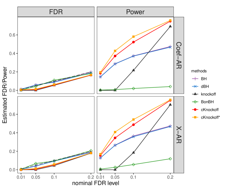
Figure 13: Estimated FDR and TPR for additional design matrix settings.

F.1.2 Cases where $m_{1}\gg 1/\alpha$

We show the performance of the procedures in the case where $\boldsymbol{\beta}$ is not too sparse. Figure 13 shows the results with $m_{1}=30$ non-null hypotheses, instead of $m_{1}=10$ in Section 6.1. The general behavior of the procedures remains the same, but

1. the power improvement of cKnockoff over knockoffs is smaller;

2. the knockoff-like methods are less powerful compared to the BH-like methods. This is because the extra power of knockoff-like methods comes from sparsity (when lasso-based feature statistics are used).

Figure 14: Estimated FDR and TPR with $30$ non-null hypotheses.

F.1.3 Comparison with multiple knockoffs

Multiple knockoffs has more implementation choices than the vanilla knockoffs, e.g. the number of knockoff variables to employ and the threshold for deciding whether the original variable “wins” the competition with its knockoffs. There is no known best choice for them, but we implement multiple knockoffs as follows:

1. We employ $5$-multiple knockoffs. That is, we generate $5$ knockoff matrices $\boldsymbol{\tilde{\boldsymbol{X}}}_{(i)}$ for $i=1,\ldots,5$ such that $\boldsymbol{X}^{\mkern-1.5mu\mathsf{T}}\boldsymbol{X}=\boldsymbol{\tilde{\boldsymbol{X}}}_{(i)}^{\mkern-1.5mu\mathsf{T}}\boldsymbol{\tilde{\boldsymbol{X}}}_{(i)}$ for all $i$ and $\boldsymbol{X}^{\mkern-1.5mu\mathsf{T}}\boldsymbol{X}-\boldsymbol{\tilde{\boldsymbol{X}}}^{\mkern-1.5mu\mathsf{T}}\boldsymbol{\tilde{\boldsymbol{X}}}_{(j)}=\boldsymbol{X}^{\mkern-1.5mu\mathsf{T}}\boldsymbol{X}-\boldsymbol{\tilde{\boldsymbol{X}}}_{(i)}^{\mkern-1.5mu\mathsf{T}}\boldsymbol{\tilde{\boldsymbol{X}}}_{(j)}$ is certain diagonal matrix for all $i\neq j$.

2. For the feature statistics, we run lasso on the augmented model

   $$\boldsymbol{y}=[\boldsymbol{X},\boldsymbol{\tilde{\boldsymbol{X}}}_{(1)},\ldots,\boldsymbol{\tilde{\boldsymbol{X}}}_{(5)}]\boldsymbol{\beta}+\boldsymbol{\varepsilon}$$

   with regularity parameter $\lambda$ determined in the same way as in LCD-T. And let

   $${\textnormal{sgn}}(W_{j})\coloneqq\begin{cases}1&\text{ if }|\hat{\beta}_{j,(0)}|>|\hat{\beta}_{j,(i)}|\text{ for all }i\in[5]\\ -1&\text{ otherwise }\end{cases},\quad\quad|W_{j}|\coloneqq\max_{i=0,\ldots,5}\left\{|\hat{\beta}_{j,(i)}|\right\},$$

   where $\hat{\beta}_{j,(i)}$ is the fitted lasso coefficient of the $i$th knockoffs of the variable $\boldsymbol{X}_{j}$ and $\hat{\beta}_{j,(0)}$ is the fitted lasso coefficient of the original variable $\boldsymbol{X}_{j}$.

To make multiple knockoffs applicable, we set $n=7m$ with $m=300$. The number of hypotheses is smaller than our usual setting, so as to save memory space in our laptop. The number of non-null hypotheses is set to be $m_{1}=30$ so as to show the performance of multiple knockoffs in the region where $m\gg 1/\alpha$.

Figure 15 shows the results. When $m_{1}<1/\alpha$, multiple knockoffs relieves the threshold phenomenon but performs worse than cKnockoff/cKnockoff^∗; when $m_{1}\gg 1/\alpha$, multiple knockoffs is even worse than the vanilla knockoffs. Moreover, multiple knockoffs does not help the whiteout phenomenon.

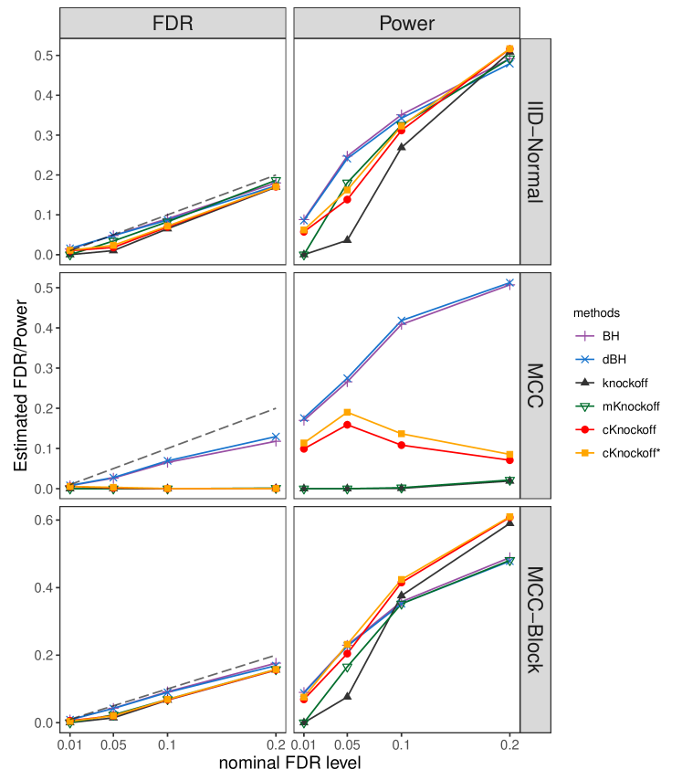
Figure 15: Estimated FDR and TPR with multiple knockoffs included.

In addition, we see the knockoff-like methods are even less powerful, compared to the BH-like methods, in Figure 15 than in Figure 14. This is because $\pi_{1}=m_{1}/m=0.1$ in this setting. That is, $\boldsymbol{\beta}$ is less sparse.

F.2 Variations of cKnockoff

Figure 16 shows the estimated FDR and power when we use C-LSM rather than LCD-T as the feature statistics. The behavior of our methods is almost the same as in Figure 4.

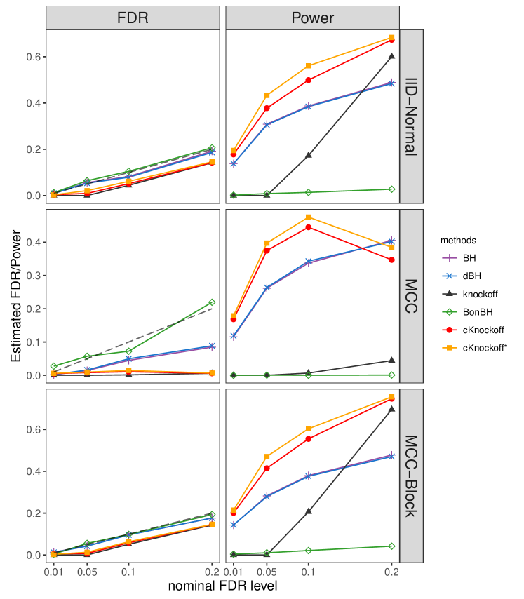
Figure 16: Estimated FDR and TPR under settings using C-LSM as the feature statistics.

F.3 Distributions of FDP and TPP

Figure 17 and 18 show the empirical cumulative distribution functions (ECDF) of the FDP and TPP, respectively, of selected procedures, under the same setting as the experiments in Section 6.1.

For FDP, we see that knockoffs, cKnockoff, and cKnockoff^∗ all work well, in the sense that the FDP is smaller than $\alpha$ with high probability in most cases. By contrast, BH and dBH both have stochastically larger FDP in all these cases even when their power is lower. In particular, in the MCC problem, the FDP distribution of BH/dBH puts large mass at both $0$ and $1$, rendering the rejection sets less reliable.

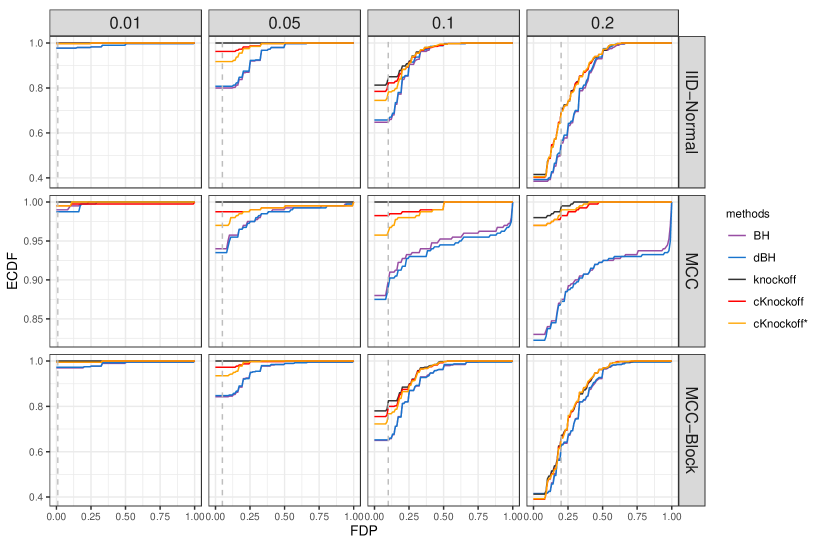
Figure 17: Empirical CDF of FDP from different procedures. Different columns represent different nominal FDR level $\alpha$, whose value is also indicated by a vertical dashed line.

For TPP, all procedures perform similarly and the TPP is not concentrated at the TPR. Moreover, when knockoffs make some rejections, cKnockoff/cKnockoff^∗ makes a bit more; and when knockoffs fails to reject anything (a flat TPP CDF towards $\text{TPP}=0$), the CDF of cKnockoff/cKnockoff^∗ keeps its trend. This indicates that our methods fully unleash the potential power of the knockoffs when it suffers.

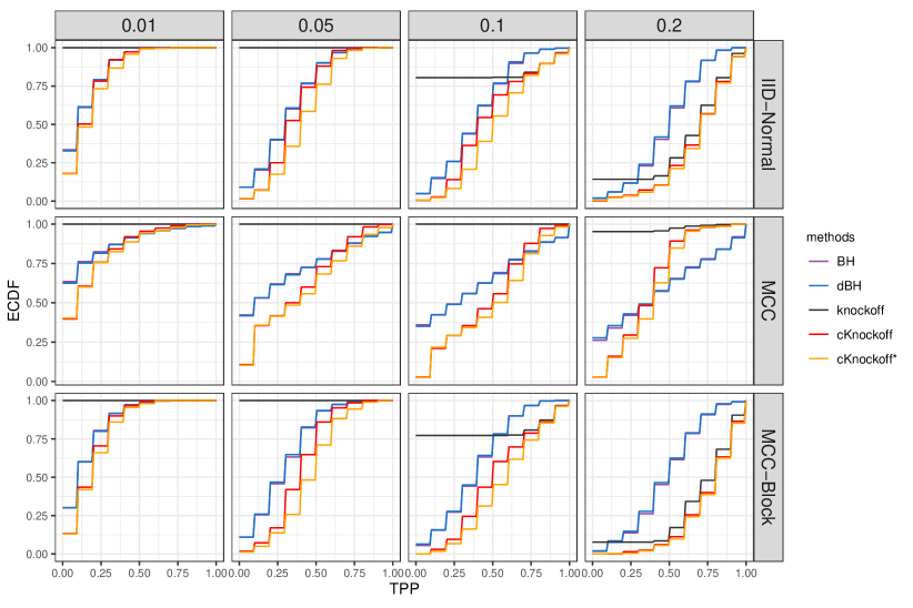
Figure 18: Empirical CDF of TPP from different procedures. Different columns represent different nominal FDR level $\alpha$.

Appendix G HIV drug resistance data

Continuing the discussion in Section 8, Figure 19 presents the results where we set $\alpha=0.2$. The knockoffs suffers in experiments like the drug AZT and D4T. Our cKnockoff and cKnockoff^∗ procedures save knockoffs in these cases and make strictly more discoveries than knockoffs in almost all cases.

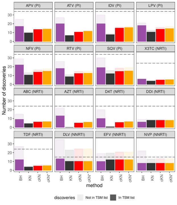
Figure 19: Results on the HIV drug resistance data with $\alpha=0.2$. The darker segments represent the number of discoveries that were replicated in the TSM panel, while the lighter segments represent the number that was not. The horizontal dashed line indicates the total number of mutations appearing in the TSM list. Results are shown for the BH, fixed-$X$ knockoffs, cKnockoff and cKnockoff^∗.

References

- Barber and Candès (2015) Rina Foygel Barber and Emmanuel J Candès. Controlling the false discovery rate via knockoffs. The Annals of Statistics, 43(5):2055–2085, 2015.
- Benjamini and Hochberg (1995) Yoav Benjamini and Yosef Hochberg. Controlling the false discovery rate: a practical and powerful approach to multiple testing. Journal of the Royal statistical society: series B (Methodological), 57(1):289–300, 1995.
- Candès et al. (2018) Emmanuel Candès, Yingying Fan, Lucas Janson, and Jinchi Lv. Panning for gold: ‘model-X’ knockoffs for high dimensional controlled variable selection. Journal of the Royal Statistical Society: Series B (Statistical Methodology), 80(3):551–577, 2018.
- Emery and Keich (2019) Kristen Emery and Uri Keich. Controlling the fdr in variable selection via multiple knockoffs. arXiv preprint arXiv:1911.09442, 2019.
- Fan et al. (2019) Yingying Fan, Emre Demirkaya, Gaorong Li, and Jinchi Lv. Rank: large-scale inference with graphical nonlinear knockoffs. Journal of the American Statistical Association, 2019.
- Fithian and Lei (2022) William Fithian and Lihua Lei. Conditional calibration for false discovery rate control under dependence. The Annals of Statistics, 50(6):3091–3118, 2022.
- Gimenez and Zou (2019) Jaime Roquero Gimenez and James Zou. Improving the stability of the knockoff procedure: Multiple simultaneous knockoffs and entropy maximization. In The 22nd International Conference on Artificial Intelligence and Statistics, pages 2184–2192. PMLR, 2019.
- Javanmard and Montanari (2014) Adel Javanmard and Andrea Montanari. Confidence intervals and hypothesis testing for high-dimensional regression. The Journal of Machine Learning Research, 15(1):2869–2909, 2014.
- Katsevich et al. (2021) Eugene Katsevich, Chiara Sabatti, and Marina Bogomolov. Filtering the rejection set while preserving false discovery rate control. Journal of the American Statistical Association, pages 1–12, 2021.
- Li and Fithian (2021) Xiao Li and William Fithian. Whiteout: when do fixed-x knockoffs fail? arXiv preprint arXiv:2107.06388, 2021.
- Liu and Rigollet (2019) Jingbo Liu and Philippe Rigollet. Power analysis of knockoff filters for correlated designs. arXiv preprint arXiv:1910.12428, 2019.
- Nguyen et al. (2020) Tuan-Binh Nguyen, Jérôme-Alexis Chevalier, Bertrand Thirion, and Sylvain Arlot. Aggregation of multiple knockoffs. In International Conference on Machine Learning, pages 7283–7293. PMLR, 2020.
- Ning and Liu (2017) Yang Ning and Han Liu. A general theory of hypothesis tests and confidence regions for sparse high dimensional models. 2017.
- Rhee et al. (2006) Soo-Yon Rhee, Jonathan Taylor, Gauhar Wadhera, Asa Ben-Hur, Douglas L Brutlag, and Robert W Shafer. Genotypic predictors of human immunodeficiency virus type 1 drug resistance. Proceedings of the National Academy of Sciences, 103(46):17355–17360, 2006.
- Romano et al. (2020) Yaniv Romano, Matteo Sesia, and Emmanuel Candès. Deep knockoffs. Journal of the American Statistical Association, 115(532):1861–1872, 2020.
- Sarkar and Tang (2021) Sanat K Sarkar and Cheng Yong Tang. Adjusting the benjamini-hochberg method for controlling the false discovery rate in knockoff assisted variable selection. arXiv preprint arXiv:2102.09080, 2021.
- Shah and Bühlmann (2023) Rajen D Shah and Peter Bühlmann. Double-estimation-friendly inference for high-dimensional misspecified models. Statistical Science, 38(1):68–91, 2023.
- Shah and Peters (2020) Rajen D Shah and Jonas Peters. The hardness of conditional independence testing and the generalised covariance measure. 2020.
- Tibshirani (1996) Robert Tibshirani. Regression shrinkage and selection via the lasso. Journal of the Royal Statistical Society: Series B (Methodological), 58(1):267–288, 1996.
- Van de Geer et al. (2014) Sara Van de Geer, Peter Bühlmann, Ya’acov Ritov, and Ruben Dezeure. On asymptotically optimal confidence regions and tests for high-dimensional models. 2014.
- Wang and Janson (2020) Wenshuo Wang and Lucas Janson. A power analysis of the conditional randomization test and knockoffs. arXiv preprint arXiv:2010.02304, 2020.
- Waudby-Smith and Ramdas (2020) Ian Waudby-Smith and Aaditya Ramdas. Estimating means of bounded random variables by betting. arXiv preprint arXiv:2010.09686, 2020.
- Weinstein et al. (2017) Asaf Weinstein, Rina Barber, and Emmanuel Candès. A power and prediction analysis for knockoffs with lasso statistics. arXiv preprint arXiv:1712.06465, 2017.
- Weinstein et al. (2020) Asaf Weinstein, Weijie J Su, Małgorzata Bogdan, Rina F Barber, and Emmanuel J Candes. A power analysis for knockoffs with the lasso coefficient-difference statistic. arXiv preprint arXiv:2007.15346, 2(7), 2020.
- Zhang and Zhang (2014) Cun-Hui Zhang and Stephanie S Zhang. Confidence intervals for low dimensional parameters in high dimensional linear models. Journal of the Royal Statistical Society Series B: Statistical Methodology, 76(1):217–242, 2014.