On computing Discretized Ricci curvatures of graphs: local algorithms and (localized) fine-grained reductions

Abstract

Characterizing shapes of high-dimensional objects via Ricci curvatures plays a critical role in many research areas in mathematics and physics. However, even though several discretizations of Ricci curvatures for discrete combinatorial objects such as networks have been proposed and studied by mathematicians, the computational complexity aspects of these discretizations have escaped the attention of theoretical computer scientists to a large extent. In this paper, we study one such discretization, namely the Ollivier-Ricci curvature, from the perspective of efficient computation by fine-grained reductions and local query-based algorithms. Our main contributions are the following.

1. We relate our curvature computation problem to minimum weight perfect matching problem on complete bipartite graphs via fine-grained reduction.

2. We formalize the computational aspects of the curvature computation problems in suitable frameworks so that they can be studied by researchers in local algorithms.

3. We provide the first known lower and upper bounds on queries for query-based algorithms for the curvature computation problems in our local algorithms framework. En route, we also illustrate a localized version of our fine-grained reduction.

We believe that our results bring forth an intriguing set of research questions, motivated both in theory and practice, regarding designing efficient algorithms for curvatures of geometrical objects.

[1]organization=Department of Computer Science, University of Illinois Chicago, city=Chicago, postcode=60607, state=IL, country=USA

[2]organization=Department of Computer Science, Purdue University, city=West Lafayette, postcode=47907, state=IN, country=USA

We relate our curvature computation problem to minimum weight perfect matching problem on complete bipartite graphs via fine-grained reduction.

We formalize the computational aspects of the curvature computation problems in suitable frameworks so that they can be studied by researchers in local algorithms.

We provide the first known lower and upper bounds on queries for query-based algorithms for the curvature computation problems in our local algorithms framework. En route, we also illustrate a localized version of our fine-grained reduction.

1 Introduction

A suitable notion of “shape” plays a critical role in investigating objects in mathematics, mathematical physics and other research areas. Various kinds of curvatures are very natural measures of shapes of higher dimensional objects in mainstream physics and mathematics [1, 2]. To quantify the shape of a higher-dimensional geometric object, one often fixes shapes of objects with specific properties as the “baseline shape” and then quantifies the shape of a given object with respect to these baseline shapes. For example, consider the case of the two-dimensional metric space. For this space, a baseline could be selected as the standard Euclidean plane in which the three angles of a triangle sum up to exactly $180^{\circ}$, and then one can quantify the shape of the given two-dimensional space by the deviations of the sum of the three angles of triangles in this space from the baseline of $180^{\circ}$. An alternative approach is to avoid selecting baseline shapes explicitly and instead directly quantify the shape of a given geometric object. Quantification of shape is often referred to as the curvature of the corresponding object. Quantification of shapes can be either local or global. A local shape of the object is usually computed for a specific local neighborhood of the object (e.g., the Ricci curvature). In contrast, a global shape of the object is usually computed over the entire object (e.g., the Gromov-hyperbolicity measure). Any attempt to extend notions of curvature measures from non-network domains to networks (and other discrete combinatorial structures) need to overcome at least three key challenges, namely that (a) networks are discrete (non-continuous) combinatorial objects, (b) networks may not necessarily have an associated natural geometric embedding, and (c) the extension need to be useful and non-trivial, i.e., a network curvature measure should saliently encode non-trivial higher-order correlations among nodes and edges that cannot be obtained by other popular network measures.

1.1 Motivations behind studying shapes of networks

Although studying measures of shapes of networks (and hypergraphs) is mathematically intriguing, it is natural to ask if there are other valid reasons for such studies. Network shape measures can encode non-trivial topological properties that are not expressed by more established network-theoretic measures such as degree distributions, clustering coefficients or betweenness centralities (e.g., see [3, 4]). Moreover, these shape measures can explain many phenomena one frequently encounters in real network-theoretic applications, such as (i) paths mediating up- or down-regulation of a target node starting from the same regulator node in biological regulatory networks often have many small crosstalk paths [3] and (ii) existence of congestions in a node that is not a hub in traffic networks [3, 5], that are not easily explained by other non-shape measures. Recently, shape measures have also found applications in traditional social networks applications such as community finding [6], and in neuroscience applications such as comparing brain networks to study slowly progressing brain diseases such as attention deficit hyperactivity disorder [4] and autism spectrum disorder [7, 8].

1.2 Brief history of existing notions of shapes for networks

There are several ways previous researchers have attempted to formulate notions of shapes of networks. Below we discuss three major directions in this regard. For further details and other approaches, the reader is referred to papers and books such as [9, 1, 10, 11, 12, 13, 14, 15, 16, 3, 17, 18, 19, 20, 21, 22, 23, 4].

One notion of network shapes, first suggested by Gromov in a non-network group theoretic context [24], is via the Gromov-hyperbolicity of networks. First defined for infinite continuous metric space [1], the measure was later adopted for finite graphs. Usually this measure is defined via properties of geodesic triangles or equivalently via $4$-node conditions, though Gromov originally defined the measure using Gromov-product nodes in [24]. Informally, any infinite metric space has a finite Gromov-hyperbolicity measure if it behaves metrically in the large scale as a negatively curved Riemannian manifold, and thus the value of this measure can be correlated to the standard scalar curvature of a hyperbolic manifold. For a finite network the measure is related to the properties of the set of exact and approximate geodesics of the network. There is a large body of research works dealing with theoretical and empirical aspects of this measure, e.g., see [14, 15, 17, 16, 18, 25] for theoretical aspects, and see [3, 5, 26] for applications to real-world networks (such as traffic congestions in a road network). Gromov-hyperbolicity is a global measure in the sense that it assigns one scalar value to the entire network.

A second notion of shape of a network can be obtained by extending Forman’s discretization of Ricci curvature for (polyhedral or CW) complexes (the “Forman-Ricci curvature”) [19] to networks. Informally, the Forman-Ricci curvature is applied to networks by topologically associating components (sub-networks) of a given network with higher-dimensional objects. The topological association itself can be carried out several ways. Although formulated relatively recently, there are already a number of papers investigating properties of these measures [20, 21, 22, 14, 23, 4].

In contrast to both of the above approaches, the network curvature considered in this paper is obtained via a discretization of curvatures from Riemannian manifolds to the network domain to capture metric properties of the manifold that are different from those captured by the Forman-Ricci curvature. More concretely, the network curvature studied in this paper is Ollivier’s earth-mover’s distances based discretization of Ricci curvature (the “Ollivier-Ricci curvature”) [10, 11, 12, 13]. For some theoretical comparison between Ollivier-Ricci curvature and Forman-Ricci curvature over graphs, see [4].

1.3 Basic definitions and notations

Let $G=(V,E)$ be a given undirected unweighted graph. The following notations related to a graph $G$ will be used subsequently:

1. $\mathsf{Nbr}_{G}(x)=\{\,y\,|\,\{x,y\}\in E\}$ and $\deg_{G}(x)=|\,\mathsf{Nbr}_{G}(x)\,|$ are the set of neighbors and the degree, respectively, of a node $x$.

2. $\mathrm{dist}_{G}(x,y)$ is the distance (i.e., number of edges in a shortest path) between the nodes $x$ and $y$ in $G$.

The following standard notations and terminologies from the field of approximation algorithms are used to facilitate further discussions:

1. ${\mathsf{OPT}}$ is the value of the objective of an optimal solution of the problem under discussion.

2. A $(\alpha,\varepsilon)$-estimate for a minimization problem under discussion is a polynomial-time algorithm that produces a solution whose objective value $\beta$ satisfies ${\mathsf{OPT}}\leq\beta\leq\alpha\,{\mathsf{OPT}}+\varepsilon$. A $(1,\varepsilon)$-estimate is also called an additive $\varepsilon$-approximation.

2 Ollivier-Ricci curvatures: intuition, definitions and simple bounds

To define the Ollivier-Ricci curvatures for the components of a graph, we first need to use the following standard definition of the earth mover’s distance (also called the $L_{1}$ Wasserstein distance) in the specific context of a edge-weighted complete bipartite graph.

Definition 1 (Earth mover’s distance (Emd) over a edge-weighted complete bipartite graph).

Let $H=(V_{L},V_{R},w)$ be an edge-weighted complete bipartite graph with $w:V_{L}\times V_{R}\mapsto{\mathbb{R}}^{+}\cup\{0\}$ being the edge-weight function, and let ${\mathbb{P}}_{L}:V_{L}\mapsto{\mathbb{R}}^{+}$ and ${\mathbb{P}}_{R}:V_{R}\mapsto{\mathbb{R}}^{+}$ be two arbitrary distributions over the nodes in $V_{L}$ and $V_{R}$, respectively. The earth mover’s distance corresponding to the distributions ${\mathbb{P}}_{L}$ and ${\mathbb{P}}_{R}$, denoted by Emd${}_{H}({\mathbb{P}}_{L},{\mathbb{P}}_{R})$ $($or simply Emd$)$, is the value of the objective function of an optimal solution of the following linear program that has a variable $z_{x,y}$ for every pair of nodes $x\in V_{L}$ and $y\in V_{R}$:

$$\boxed{\text{ \begin{tabular}[]{ r l }\emph{minimize}&$\sum_{x\in V_{L}}\sum_{y\in V_{R}}w(x,y)\,z_{x,y}$\\[5.0pt] \emph{subject to}&$\sum_{y\in V_{R}}z_{x,y}={\mathbb{P}}_{L}(x),\,\,$ for all $x\in V_{L}$\\[5.0pt] &$\sum_{x\in V_{L}}z_{x,y}={\mathbb{P}}_{R}(y),\,\,$ for all $y\in V_{R}$\\[5.0pt] &$z_{x,y}\geq 0,\,\,$ for all $x\in V_{L}$ and $y\in V_{R}$\end{tabular} }}$$ (5)

Let $G=(V,E)$ be an undirected unweighted graph. Consider an edge $e=\{u,v\}\in E$. Define the edge-weighted complete bipartite graph $G_{u,v}=(L_{u,v}^{G},R_{u,v}^{G},w_{u,v}^{G})$ as follows:

1. $L_{u,v}^{G}=\{u\}\cup\mathsf{Nbr}_{G}(u)$,

2. $R_{u,v}^{G}=\{v\}\cup\mathsf{Nbr}_{G}(v)$, and

3. the edge-weight function $w_{u,v}^{G}$ is given by $w_{u,v}^{G}(u^{\prime},v^{\prime})=\mathrm{dist}_{G}(u^{\prime},v^{\prime})$ for all $u^{\prime}\in L_{u,v}^{G},v^{\prime}\in R_{u,v}^{G}$.

Let ${\mathbb{P}}_{u}^{G}$ and ${\mathbb{P}}_{v}^{G}$ denote the two uniform distributions over the nodes in $L_{u,v}^{G}$ and $R_{u,v}^{G}$, respectively, i.e.,

$$\forall\,x\in L_{u,v}^{G}:\,{\mathbb{P}}_{u}^{G}(x)=\frac{1}{1+\deg_{G}(u)}$$

$$\forall\,x\in R_{u,v}^{G}:\,{\mathbb{P}}_{v}^{G}(x)=\frac{1}{1+\deg_{G}(v)}$$

We can now state the precise definitions of the curvatures used in this paper.

1. The Ollivier-Ricci curvature of the edge $\boldsymbol{e=\{u,v\}}$ of $G$ is defined as [10]

   $$\boxed{\mathfrak{C}_{G}(e)\stackrel{{\scriptstyle\mathrm{def}}}{{=}}\mathfrak{C}_{G}(u,v)=1-\text{{\sc Emd}}_{\!\!\!G_{u,v}}({\mathbb{P}}_{u}^{G},{\mathbb{P}}_{v}^{G})}$$ (6)

2. The Ollivier-Ricci curvature of a node $\boldsymbol{v}$ is calculated by taking the average of the Ollivier-Ricci curvatures of all the edges incident on $v$, i.e.,

   $$\boxed{\mathfrak{C}_{G}(v)=\frac{1}{\deg_{G}(v)}\sum_{e=\{u,v\}\in E}\mathfrak{C}_{G}(e)}$$ (7)

3. Finally, the average Ollivier-Ricci curvature of a graph $\boldsymbol{G}$ is calculated by taking the average of the Ollivier-Ricci curvatures of all the edges in $G$, i.e.,

   $$\boxed{\mathfrak{C}_{\mathrm{avg}}(G)=\frac{1}{|E|}\sum_{e\in E}\mathfrak{C}_{G}(e)}$$ (8)

For easy quick reference, we explicitly write below the version of the linear program in (5) as used in the calculation of $\mathfrak{C}_{G}(u,v)$:

minimize $$\sum_{x\in\{u\}\cup\mathsf{Nbr}_{G}(u)}\sum_{y\in\{v\}\cup\mathsf{Nbr}_{G}(v)}\mathrm{dist}_{G}(x,y)\,z_{x,y} \sum_{y\in\{v\}\cup\mathsf{Nbr}_{G}(v)}z_{x,y}=\frac{1}{1+\deg_{G}(u)},\,\, x\in\{u\}\cup\mathsf{Nbr}_{G}(u) \sum_{x\in\{u\}\cup\mathsf{Nbr}_{G}(u)}z_{x,y}=\frac{1}{1+\deg_{G}(u)},\,\, y\in\{v\}\cup\mathsf{Nbr}_{G}(v) z_{x,y}\geq 0,\,\, x\in\{v\}\cup\mathsf{Nbr}_{G}(v) y\in\{u\}\cup\mathsf{Nbr}_{G}(u) \mathsf{LP} \mathfrak{C}_{G}$$ subject to         for all         for all         for all and (-)

Assuming $\deg_{G}(u)\leq\deg_{G}(v)$, the linear program in ($\mathsf{LP}$-$\mathfrak{C}_{G}$) has $\deg_{G}(u)\allowbreak\times\allowbreak\deg_{G}(v)\allowbreak=\allowbreak O((\deg_{G}(v))^{2})$ variables and $\deg_{G}(u)+\deg_{G}(v)\leq 2\,\deg_{G}(v)$ constraints. The best time-complexity for solving the linear program in ($\mathsf{LP}$-$\mathfrak{C}_{G}$) can be estimated as follows:

1. Based on the state-of-the-art algorithms for solving linear program for this situation [28], an exact solution of ($\mathsf{LP}$-$\mathfrak{C}_{G}$) can be found in $O((\deg_{G}(v))^{5/2})$ time.

2. Based on the results in publications such as [29, 30], an additive $\varepsilon$-approximation of ($\mathsf{LP}$-$\mathfrak{C}_{G}$) can be obtained in $\tilde{O}\big{(}\frac{1}{\varepsilon^{2}}\deg_{G}(u)\deg_{G}(v)\big{)}=\tilde{O}\big{(}\frac{1}{\varepsilon^{2}}(\deg_{G}(v))^{2}\,\big{)}$ time.

The following observation is crucial for this paper.

Observation 1.

The values $\mathrm{dist}_{G}(x,y)$ in the linear program in ($\mathsf{LP}$-$\mathfrak{C}_{G}$) satisfy the property that $\mathrm{dist}_{G}(x,y)\in\{0,1,2,3\}$.

It is not difficult to see that Observation 1 implies $0\leq\text{{\sc Emd}}_{\!\!\!G_{u,v}}({\mathbb{P}}_{u}^{G},{\mathbb{P}}_{v}^{G})\leq 3$ and therefore $-2\leq\mathfrak{C}_{G}(e)\leq 1$. For computing $\mathfrak{C}_{G}(u,v)$ and related quantities, we assume that $\boldsymbol{\deg_{G}(u)\leq\deg_{G}(v)}$ without any loss of generality throughout the rest of the paper. Moreover, we also assume without loss of generality that $\boldsymbol{\deg_{G}(v)=\omega(1)}$ since otherwise $\boldsymbol{\text{{\sc Emd}}_{\!\!\!G_{u,v}}({\mathbb{P}}_{u}^{G},{\mathbb{P}}_{v}^{G})}$ can be computed in $\boldsymbol{O(1)}$ time.

2.1 Intuition behind the discretization resulting in definition of $\mathfrak{C}_{G}(e)$

For an intuitive understanding of the definition of $\mathfrak{C}_{G}(e)$, we recall the notion of Ricci curvature for a smooth Riemannian manifold. The Ricci curvature at a point $x$ in the manifold along a direction can be thought of transporting a small ball centered at $x$ along that direction and measuring the “distortion” of that ball due to the shape of the surface by comparing the distance between the two small balls with the distance between their centers. In the definition of $\mathfrak{C}_{G}(e)$, the role of the direction is captured by the edge $e=\{u,v\}$, the roles of the balls at the two points are played by the two closed neighborhoods $L_{u,v}^{G}$ and $R_{u,v}^{G}$, and the role of the distance between the two balls is captured by the earth mover’s distance between the two distributions ${\mathbb{P}}_{u}^{G}$ and ${\mathbb{P}}_{v}^{G}$ over the nodes in $L_{u,v}^{G}$ and $R_{u,v}^{G}$ on the metric space of shortest paths in $G$. For further intuition, see publications such as [10]. The Forman-Ricci curvature also assigns a number to each edge of the given graph, but the numbers are calculated in quite a different way from that in the Ollivier-Ricci curvature to capture different metric properties of the manifold.

2.2 Equivalent reformulation of linear program ($\mathsf{LP}$-$\mathfrak{C}_{G}$) when $\deg_{G}(u)=\deg_{G}(v)$

The following claim holds based on results in prior publications such as [31, 32]. For the convenience of the reader, we provide a self-contained proof in the appendix.

Fact 1.

[31, 32] If $\deg_{G}(u)=\deg_{G}(v)$ then the following claims are true regarding some optimal solution of the linear program ($\mathsf{LP}$-$\mathfrak{C}_{G}$):

1. The values of the variables $z_{u^{\prime},v^{\prime}}$ are either $0$ or $\frac{1}{\deg_{G}(v)}$.

2. The edges in $\left\{\,\{u^{\prime},v^{\prime}\}\,|\,z_{u^{\prime},v^{\prime}}=\frac{1}{\deg_{G}(v)}\,\right\}$ form a minimum-weight perfect matching in $G_{u,v}$ that uses the zero-weight edges $\{u^{\prime},u^{\prime}\}$ for all $u^{\prime}\in\{u,v\}\cup\big{(}\,\mathsf{Nbr}_{G}(u)\cap\mathsf{Nbr}_{G}(v)\,\big{)}$.

Based on Fact 1, for the case when when $\deg_{G}(u)=\deg_{G}(v)$ an optimal solution of the linear program ($\mathsf{LP}$-$\mathfrak{C}_{G}$) can be obtained by finding a minimum-weight perfect matching for a complete edge-weighted bipartite graph $H=(L,R,w)$ where

1. $L=\mathsf{Nbr}_{G}(u)\setminus\big{(}\mathsf{Nbr}_{G}(v)\cup\{v\}\big{)}$,

2. $R=\mathsf{Nbr}_{G}(v)\setminus\big{(}\mathsf{Nbr}_{G}(u)\cup\{u\}\big{)}$, and

3. the edge-weight function $w:L\times R\mapsto\{1,2,3\}$ is given by $w(x,y)=\mathrm{dist}_{G}(x,y)$.

Note that $|L|=|R|=\deg_{G}(v)-1-|\mathsf{Nbr}_{G}(u)\cap\mathsf{Nbr}_{G}(v)|$. Letting $\mathcal{M}(H)\in\{|R|,|R|+1,\dots,3\,|R|\}$ denote the total weight of a minimum-weight perfect matching of $H$, we have

$$\mathfrak{C}_{G}(e)=1-\frac{\mathcal{M}(H)}{1+\deg_{G}(v)}$$

Proposition 1.

An additive $\varepsilon|R|$-approximation of $\mathcal{M}(H)$ implies an additive $\varepsilon$-approximation of $\mathfrak{C}_{G}(e)$, and vice versa.

Proof.

This follows from the facts that $|R|\leq\mathcal{M}(H)\leq 3\,|R|$ and $\deg_{G}(v)>|R|$. ∎

2.3 Some simple bounds for $\text{{\sc Emd}}_{\!\!\!G_{u,v}}({\mathbb{P}}_{u},{\mathbb{P}}_{v})$ and $\mathfrak{C}_{G}(e)$

We use a calculation similar to the one used in [31]. Extend the distributions ${\mathbb{P}}_{u}^{G}$ and ${\mathbb{P}}_{v}^{G}$ to ${\mathbb{P}}_{u}^{G^{\prime}}$ and ${\mathbb{P}}_{v}^{G^{\prime}}$ over $L_{u,v}^{G}\cup R_{u,v}^{G}$ by letting ${\mathbb{P}}_{u}^{G^{\prime}}(x)=0$ for $x\in R_{u,v}\setminus L_{u,v}$ and ${\mathbb{P}}_{v}^{G^{\prime}}(x)=0$ for $x\in L_{u,v}\setminus R_{u,v}$. For notational simplicity, let $k=\mathsf{Nbr}_{G}(u)\setminus\mathsf{Nbr}_{G}(v)$, $\ell=\mathsf{Nbr}_{G}(u)\cap\mathsf{Nbr}_{G}(v)$, and $m=\mathsf{Nbr}_{G}(v)\setminus\mathsf{Nbr}_{G}(u)$, thus $\deg_{G}(u)=k+\ell$ and $\deg_{G}(v)=m+\ell$. By straightforward calculation, the total variation distance (TVD) between ${\mathbb{P}}_{u}^{\prime}$ and ${\mathbb{P}}_{v}^{\prime}$ is

$$\textstyle||\,{\mathbb{P}}_{u}^{\prime}-{\mathbb{P}}_{v}^{\prime}\,||_{\mathrm{TVD}}=\frac{1}{2}\times\left(\frac{k-1}{k+\ell+1}+\frac{m-1}{m+\ell+1}+(\ell+2)\times\left(\frac{1}{k+\ell+1}-\frac{1}{m+\ell+1}\right)\right)\\ \textstyle=1-\frac{\ell+2}{\deg(v)+1}$$

Since $1\leq\mathrm{dist}_{G}(u^{\prime},v^{\prime})\leq 3$ for all $u^{\prime},v^{\prime}\in L_{u,v}^{G}\cup R_{u,v}^{G},u^{\prime}\neq v^{\prime}$, by standard relationships between Emd and TVD (e.g., see [33]) it follows that $||\,{\mathbb{P}}_{u}^{\prime}-{\mathbb{P}}_{v}^{\prime}\,||_{\mathrm{TVD}}\leq\text{{\sc Emd}}_{\!\!\!G_{u,v}}({\mathbb{P}}_{u},{\mathbb{P}}_{v})\leq 3\times||\,{\mathbb{P}}_{u}^{\prime}-{\mathbb{P}}_{v}^{\prime}\,||_{\mathrm{TVD}}$, thereby giving

$$-2+\frac{3\ell+6}{\deg_{G}(v)+1}\leq\mathfrak{C}_{G}(e)\leq\frac{\ell+2}{\deg_{G}(v)+1}$$

Furthermore, if $G$ has no cycles of length $5$ or less containing $e$ then $\mathrm{dist}_{G}(u^{\prime},v^{\prime})=3$ for all $u^{\prime},v^{\prime}\in L_{u,v}^{G}\cup R_{u,v}^{G}$ and $\ell=0$ giving $\mathfrak{C}_{G}(e)=\frac{2}{\deg_{G}(v)+1}$.

3 Synopsis of our results

The main goal of this paper is to study algorithmic complexities of efficient computation of our network curvature measures. To this effect, our main contributions are threefold:

1. We relate various cases of our curvature computation problems via fine-grained reduction.

2. We formalize the computational aspects of the curvature computation problems in suitable frameworks so that they can be studied by researchers in local algorithms.

3. We provide the first known lower and upper bounds on queries for query-based algorithms for the curvature computation problems in our local algorithms framework. En route, we also illustrate a localized version of our fine-grained reduction.

A summary of our contribution in the rest of this paper is the following.

1. In Section 4 we relate via Theorem 3 the minimum weight perfect matching problem on complete bipartite graphs with ternary weights to computing $\mathfrak{C}_{G}(e)$ via fine-grained reduction.

2. In Section 5 we present our results for computing $\mathfrak{C}_{G}(e)$ in the framework of local algorithms.

   1. In Sections 5.1 – 5.2 we provide details of the query models relevant to our case and prior related works on these query models.

   2. In Sections 5.4 – 5.6 Theorem 4, Theorem 5 and Theorem 6 provide query bounds for exact or approximate calculations of the curvature using the query models. The bounds are succinctly summarized in Section 5.3 via Table 1.

3. In Section 6 Lemma 8 provides our results for computing the Ollivier-Ricci curvature $\mathfrak{C}_{G}(v)$ for nodes and for computing the average Ollivier-Ricci curvature $\mathfrak{C}_{\mathrm{avg}}(G)$ for graphs using “black box” additive approximation algorithms for $\mathfrak{C}_{G}(e)$ and neighbor queries.

4. We conclude in Section 7 with some possible future research problems.

4 Fine-grained reduction: relating minimum weight perfect matching on complete bipartite graphs to computing $\mathfrak{C}_{G}(e)$

Frameworks for characterizing polynomial-time solvable problems via fine-grained reduction have garnered considerable attention in recent years (e.g., see [34] for a survey and [35, 36, 37] for a few well-known results in this direction). Essentially these fine-grained reductions are used to show that, given two problems $\mathcal{A}$ and $\mathcal{B}$ and two constants $a,b>0$, if an instance $\mathcal{I}_{\mathcal{B}}$ of size $|\mathcal{I}_{\mathcal{B}}|$ of problem $\mathcal{B}$ can be solved in $O(|\mathcal{I}_{\mathcal{B}}|^{b})$ time then an instance $\mathcal{I}_{\mathcal{A}}$ of size $|\mathcal{I}_{\mathcal{A}}|$ of problem $\mathcal{A}$ can be solved in $O(|\mathcal{I}_{\mathcal{A}}|^{a})$ time.

To begin, we first formally state the minimum weight perfect matching problem on complete bipartite graphs with ternary edge weights.

Definition 2 (minimum weight perfect matching on complete bipartite graphs with ternary weights (Mpmct)).

Given a complete edge-weighted bipartite graph $H=(A,B,w)$ where $|A|=|B|$ and $w:A\times B\mapsto\{1,2,3\}$ is the edge-weight function, find the value of $\frac{|\mathcal{M}|}{|A|}$ where $|\mathcal{M}|$ is the value $($sum of weights of edges$)$ in a minimum-weight perfect matching $\mathcal{M}$ of $H$.

For Mpmct, exact solution takes $O(|A|^{5/2})$ time [28], and an $\varepsilon$-additive approximation takes $\tilde{O}\big{(}\frac{1}{\varepsilon^{2}}|A|^{2}\,\big{)}$ time. The following theorem related Mpmct to the problem of computing a solution of the linear program in ($\mathsf{LP}$-$\mathfrak{C}_{G}$) via a fine-grained reduction.

Theorem 3.

Suppose that we have an algorithm $\mathfrak{A}$ that provides $(\alpha,\varepsilon)$-estimate for Mpmct in $O(|A|^{2+\mu})$ time for some $\mu\geq 0$ for a given input instance $H=(A,B,w)$.

Then, there exists an algorithm $\mathfrak{A}_{<}$ that provides the following estimates for the linear program in ($\mathsf{LP}$-$\mathfrak{C}_{G}$) in $O(\deg_{G}(v)^{2+\mu})$ time:

1. $(\alpha,\varepsilon)$-estimate if $\deg_{G}(v)+1$ is an integral multiple of $\deg_{G}(u)+1$, and

2. $(\alpha,\varepsilon+\delta)$-estimate $($for $\delta>0)$ provided $\delta$ satisfies at least one of the following conditions:

   1. $\deg_{G}(u)\leq(\delta/3)\times\deg_{G}(v)$, or

   2. $\deg_{G}(u)\geq(1-(\delta/3)\,)\times\deg_{G}(v)$.

Remark 1.

An illustration of the result in Theorem 3 is as follows. Suppose that we can solve Mpmct exactly in $O(|A|^{2.4})$ time $($implying $\alpha=1$ and $\varepsilon=0)$. Then, such an algorithm can be used to obtain a ${\deg_{G}(v)}^{-1/2}$-additive approximation of ($\mathsf{LP}$-$\mathfrak{C}_{G}$) (i.e., $\delta={\deg_{G}(v)}^{-1/2})$ in $O((\deg_{G}(v))^{2.4})$ time provided at least one of the following conditions hold: (a) $\deg_{G}(u)\leq\frac{\sqrt{\deg_{G}(v)}}{3}$, (b) $\deg_{G}(u)\geq\deg_{G}(v)-\frac{\sqrt{\deg_{G}(v)}}{3}$, or (c) $\deg_{G}(v)+1$is an integral multiple of $\deg_{G}(u)+1$. Such a result will improve the best possible running time for a ${\deg_{G}(v)}^{-1/2}$-additive approximation of ($\mathsf{LP}$-$\mathfrak{C}_{G}$).

Proof.

Let $\mathsf{Nbr}_{G}(u)\cup\{u\}=\{x_{1},\dots,x_{\deg(u)+1}\}$, and $\mathsf{Nbr}_{G}(v)\cup\{v\}=\{y_{1},\dots,y_{\deg(v)+1}\}$, where $x_{\deg_{G}(u)}=y_{\deg_{G}(v)}=u$ and $x_{\deg_{G}(u)+1}=y_{\deg_{G}(v)+1}=v$. Let $\deg_{G}(v)+1=a\,(\deg_{G}(u)+1)+b$ for two integers $a\geq 1$ and $0\leq b<\deg_{G}(u)+1$. We construct a new graph $G_{u,v}^{\prime}=(L_{u,v}^{G^{\prime}},R_{u,v}^{G^{\prime}},w_{u,v}^{G^{\prime}})$ from $G_{u,v}$ in the following manner:

1. We set $R_{u,v}^{G^{\prime}}=R_{u,v}^{G}$.

2. Every node $x_{i}$ is replaced by $a$ nodes $x_{i}^{1},\dots,x_{i}^{a}$ in $L_{u,v}^{G^{\prime}}$. Moreover, we have $b$ additional “special” nodes $r_{1},\dots,r_{b}$ in $L_{u,v}^{G^{\prime}}$. Note that after these modifications $|L_{u,v}^{G^{\prime}}|=|R_{u,v}^{G^{\prime}}|=1+\deg_{G}(v)$.

3. We set the new weights $w_{u,v}^{G^{\prime}}$ as follows:

   $$w_{u,v}^{G^{\prime}}(x_{i}^{j},y_{\ell}) = \mathrm{dist}_{G}(x_{i},y_{\ell})\text{ for $i\in\{1,\dots,\deg_{G}(u)+1\}$,}$$

   $$j\in\{1,\dots,a\} \ell\in\{1,\dots,\deg_{G}(v)+1\}$$, and

   $$w_{u,v}^{G^{\prime}}(r_{i},y_{\ell}) = 3\text{ for $i\in\{1,\dots,b\}$, and $\ell\in\{1,\dots,\deg_{G}(v)+1\}$}$$

4. The two new probability distributions ${{\mathbb{P}}_{u}}^{\!\!\!\!G_{u,v}^{\prime}}$ and ${{\mathbb{P}}_{v}}^{\!\!\!\!G_{u,v}^{\prime}}$ over the nodes in $L_{u,v}^{G^{\prime}}$ and $R_{u,v}^{G^{\prime}}$ are as follows: ${{\mathbb{P}}_{v}}^{\!\!\!\!G_{u,v}^{\prime}}(x)={\mathbb{P}}_{v}^{G}(x)$ for all $x\in\{y_{1},\dots,y_{\deg_{G}(v)+1}\}$, and ${{\mathbb{P}}_{u}}^{\!\!\!\!G_{u,v}^{\prime}}(x)=\frac{1}{1+\deg_{G}(v)}$ for all $x\in\bigcup_{i,j}\{x_{i}^{j}\}\,\cup\{r_{1},\dots,r_{b}\}$.

Since $|L_{u,v}^{G^{\prime}}|=|R_{u,v}^{G^{\prime}}|=1+\deg_{G}(v)$, using the reformulations as discussed in Section 2.2 it follows that $G_{u,v}^{\prime}$ is a valid instance $H=(A,B,w)$ of Mpmct with $|A|=\deg_{G}(v)+1$ and $w(p,q)=w_{u,v}^{G^{\prime}}(p,q)$. Note that building the graph $G_{u,v}^{\prime}$ takes $O((\deg_{G}(v))^{2})$ time, and algorithm $\mathfrak{A}$ provides a $(\alpha,\varepsilon)$-estimate for $\text{{\sc Emd}}_{\!\!G_{u,v}^{\prime}}({{\mathbb{P}}_{u}}^{\!\!\!\!G_{u,v}^{\prime}},{{\mathbb{P}}_{v}}^{\!\!\!\!G_{u,v}^{\prime}})$ in $O((\deg_{G}(v))^{2+\mu})$ time. Thus, to complete the proof it suffices to show that

$$\text{{\sc Emd}}_{\!\!\!G_{u,v}}({\mathbb{P}}_{u}^{G},{\mathbb{P}}_{v}^{G})\leq\text{{\sc Emd}}_{\!\!G_{u,v}^{\prime}}({{\mathbb{P}}_{u}}^{\!\!\!\!G_{u,v}^{\prime}},{{\mathbb{P}}_{v}}^{\!\!\!\!G_{u,v}^{\prime}})\leq\text{{\sc Emd}}_{\!\!\!G_{u,v}}({\mathbb{P}}_{u}^{G},{\mathbb{P}}_{v}^{G})+\delta$$

The linear program for $\text{{\sc Emd}}_{\!\!G_{u,v}^{\prime}}({{\mathbb{P}}_{u}}^{\!\!\!\!G_{u,v}^{\prime}},{{\mathbb{P}}_{v}}^{\!\!\!\!G_{u,v}^{\prime}})$ is a straightforward modified version of ($\mathsf{LP}$-$\mathfrak{C}_{G}$) with appropriate change of subscripts of the variables. We will refer to this modified version by ($\mathsf{LP}$-$\mathfrak{C}_{G}$)^′.

We can show $\text{{\sc Emd}}_{\!\!\!G_{u,v}^{\prime}}({{\mathbb{P}}_{u}}^{\!\!\!\!G_{u,v}^{\prime}},{{\mathbb{P}}_{v}}^{\!\!\!\!G_{u,v}^{\prime}})\leq\text{{\sc Emd}}_{\!\!\!G_{u,v}}({\mathbb{P}}_{u}^{G},{\mathbb{P}}_{v}^{G})+\delta$ as follows. Consider an optimal solution of the linear program ($\mathsf{LP}$-$\mathfrak{C}_{G}$) of value $\text{{\sc Emd}}_{\!\!\!G_{u,v}}({\mathbb{P}}_{u}^{G},{\mathbb{P}}_{v}^{G})$. From this solution we can create a feasible solution of the linear program ($\mathsf{LP}$-$\mathfrak{C}_{G}$)^′ in the following manner.

1. For $i=1,\dots,\deg_{G}(u)+1$ and $j=1,\dots,\deg_{G}(v)+1$, if $z_{x_{i},y_{j}}>0$ then distribute the value of $z_{x_{i},y_{j}}$ among the corresponding variables of ($\mathsf{LP}$-$\mathfrak{C}_{G}$)^′ as follows:

   • Repeatedly select a variable from $\{x_{i}^{1},\dots,x_{i}^{a}\}$, say $x_{i}^{\ell}$, such that $x_{i}^{\ell}<\frac{1}{1+\deg_{G}(v)}$. Increase $x_{i}^{\ell}$ to $\min\left\{\frac{1}{(1+\deg_{G}(v))},\,z_{x_{i},y_{j}}\right\}$, and decrease $z_{x_{i},y_{j}}$ by the amount by which $x_{i}^{\ell}$ was increased. Note that $w_{u,v}^{G^{\prime}}(x_{i},y_{j})=\mathrm{dist}_{G}(x_{i},y_{j})$. Repeat this step until $z_{x_{i},y_{j}}$ becomes zero or no such variable $x_{i}^{\ell}$ exists.

   • If $z_{x_{i},y_{j}}>0$ after the previous step ends then execute the following steps. Repeatedly select a variable from $\{r_{1},\dots,r_{b}\}$, say $r_{\ell}$, such that $r_{\ell}<\frac{1}{1+\deg_{G}(v)}$. Increase $r_{\ell}$ to $\min\left\{\frac{1}{(1+\deg_{G}(v))},\,z_{x_{i},y_{j}}\right\}$, and decrease $z_{x_{i},y_{j}}$ by the amount by which $r_{\ell}$ was increased. Note that $w_{u,v}^{G^{\prime}}(x_{i},y_{j})\leq\mathrm{dist}_{G}(x_{i},y_{j})+3$. Repeat this step until $z_{x_{i},y_{j}}$ becomes zero.

A straightforward calculation show that $\text{{\sc Emd}}_{\!\!\!G_{u,v}^{\prime}}({{\mathbb{P}}_{u}}^{\!\!\!\!G_{u,v}^{\prime}},{{\mathbb{P}}_{v}}^{\!\!\!\!G_{u,v}^{\prime}})\leq\text{{\sc Emd}}_{\!\!\!G_{u,v}}({\mathbb{P}}_{u}^{G},{\mathbb{P}}_{v}^{G})+\frac{3b}{\deg_{G}(v)+1}$. Therefore it suffices if we have $\frac{3b}{\deg(v)+1}\leq\delta$. If $\deg_{G}(u)+1$ is an integral multiple of $\deg_{G}(v)+1$ then $b=0$ and this proves the claim in (i). Otherwise, since $b<\deg_{G}(u)+1\leq\deg_{G}(v)+1$ and $b\leq(\deg_{G}(v)+1)-(\deg_{G}(u)+1)=\deg_{G}(v)-\deg_{G}(u)$ we get

$$\textstyle\deg_{G}(u)\leq(\delta/3)\times\deg_{G}(v)\,\Rightarrow\,b<\deg_{G}(u)+1\leq(\delta/3)\times\deg_{G}(v)+1\\ \textstyle\Rightarrow\,\frac{3b}{\deg(v)+1}<\frac{\delta\times\deg_{G}(v)+1}{\deg(v)+1}\leq\delta$$

$$\textstyle\deg_{G}(u)\geq(1-(\delta/3)\,)\times\deg_{G}(v)\,\Rightarrow\,\deg_{G}(v)-\deg_{G}(u)\leq(\delta/3)\times\deg_{G}(v)\\ \textstyle\Rightarrow\,\frac{3b}{\deg(v)+1}\leq\frac{\delta\times\deg_{G}(v)}{\deg(v)+1}<\delta$$

The proof of $\text{{\sc Emd}}_{\!\!\!G_{u,v}}({\mathbb{P}}_{u}^{G},{\mathbb{P}}_{v}^{G})\leq\text{{\sc Emd}}_{\!\!G_{u,v}^{\prime}}({{\mathbb{P}}_{u}}^{\!\!\!\!G_{u,v}^{\prime}},{{\mathbb{P}}_{v}}^{\!\!\!\!G_{u,v}^{\prime}})$ is similar. ∎

5 Computing $\mathfrak{C}_{G}(e)$ in the framework of local algorithms

By now designing local algorithms for efficient solution of graph-theoretic problems has become a well-established research area in theoretical computer science and data mining with a large body of publications (e.g., see [38, 27, 39]). A basic idea behind many of these algorithms is to suitably sample a small “local” neighborhood of the graph to infer the value of some non-local property of a graph. Frameworks for graph-theoretic applications of local algorithms hinges on the following two premises:

1. We assume that our algorithm has a list of all nodes in the graph in a suitable format that allows for sampling a node based on some distribution.

2. The edges and their weights are not known to our algorithm a priori. Instead, the algorithm uses a “query” on a node or a pair of nodes to discover an edge and its weight. Different query models for local algorithms arise based on what kind of queries are allowed. Later in Section 5.2 we will provide details of query models that are applicable to our problems.

3. The performance of the algorithm is measured by the number of queries used.

Additional notations and conventions

For the case when $\deg_{G}(u)=\deg_{G}(v)$, we will use the reformulations of the linear program ($\mathsf{LP}$-$\mathfrak{C}_{G}$) as discussed in Section 2.2 and the associated notations contained therein. We will use the following additional notations and conventions related to the graph $H=(L,R,w)$ mentioned in Section 2.2:

1. $|L|=|R|=n$, $L=\{u_{1},\dots,u_{n}\}$ and $R=\{v_{1},\dots,v_{n}\}$.

2. For $j\in\{1,2\}$ $\deg_{H,j}(x)$ denotes the number of edges of weight $j$ incident on node $x$ in a graph $H$.

Note that $\boldsymbol{H}$ has $\boldsymbol{2n}$ nodes. Moreover, for any edge-weighted graph $F=(V,E,w)$ with $w:E\mapsto{\mathbb{R}}$, $\mbox{wt-}\deg_{F}(u)=\sum_{v:\{u,v\}\in E}w(u,v)$ denotes the weighted degree of node $u$ in $F$, and $\mathcal{M}(F)$ denotes the total weight of a minimum-weight perfect matching of $F$.

5.1 Prior related works

Designing sublinear time and sketching algorithms for the general earth mover’s distance on the shortest path metric for arbitrary graphs have been investigated in prior research papers such as [40, 41]. In particular, for an edge-weighted tree with $W$ being the maximum weight of any edge and for any two unknown probability distributions on the nodes, the authors in [40] show that an estimate of the Emd with $\varepsilon$-additive error can be achieved by using $\tilde{O}(\frac{W^{2}n^{2}}{\varepsilon^{2}})$ samples from the two distributions and observes that their algorithm is optimal up to polylog factors. To the best of our knowledge, local algorithms for computing the Ollivier-Ricci curvatures of a graph have not been investigated explicitly before.

5.2 Query models for edge-weighted complete bipartite graphs

Two standard query models that appear in the local algorithms literature for unweighted graphs (e.g., see [38]) are as follows: the node-pair query model (the query is a pair of nodes and the answer is whether an edge between them exists or not), and the neighbor query model (the query is a node and the answer is a random not-yet-explored adjacent node if it exists). Since our given graph is an edge-weighted complete bipartite graph $H=(L,R,w)$ via the reformulation described in Section 2.2, natural extensions lead to the following query models for our case:

1. weighted node-pair query model: the query is a pair of nodes $x,y$ and the answer is the weight $w(x,y)$.

2. neighbor query model: the query is a node $x$ and the answer is a random “not-yet-explored” node adjacent to $x$ (if no such node exists then the query returns a special symbol to indicate that). Note that such a query does not give any useful information $($beyond simply picking a node uniformly at random$)$ for the graph $H$ since it is a complete graph. We will only use this type of query for the entire given graph $G$ for computing $\mathfrak{C}_{G}(v)$ and $\mathfrak{C}_{\mathrm{avg}}(G)$ in Section 6.

3. weighted neighbor query model: the query is $(x,y)$ where $x$ is a node and $y$ is a number, and the answer is a random “not-yet-explored” node $z$ such that $w(x,z)=y$ (if no such node exists then the query returns a special symbol to indicate that).

4. weighted selective degree query model: the query is $(x,y)$ where $x$ is a node and $y$ is a number, and the answer is the number of edges of weight $y$ that are incident on $x$.

5.3 Summary of our query bounds on computing $\mathfrak{C}_{G}(e)$

For the convenience of the reader, we summarize our query bounds for computing $\mathfrak{C}_{G}(e)$ in Table 1. Subsequent sub-sections in this section provide proofs of these bounds.

	query	additive	expected	result(s)	additional
	types	approx.	# of queries		remark(s)
lower bounds {5*	weighted node-pair	exact computation	$>\frac{(\deg_{G}(v)-1)^{2}}{6}$	Theorem 4(a)-(i)	]5*[①]
	weighted neighbor	exact computation	$>\frac{\deg_{G}(v)-1}{2}$	Theorem 4(a)-(ii)
	weighted node-pair	$2-\varepsilon_{1}$	$>\frac{\deg_{G}(v)-1}{6}$	Theorem 4(b)
upper bounds {7*	weighted neighbor	$1+\varepsilon_{2}$	$O(1)$	Theorem 5(a)	②
	weighted neighbor	$\frac{1}{2}+\varepsilon_{2}$	$O(1)$	Theorem 5(b)	③
	weighted neighbor	$1+\varepsilon_{2}+\delta$	$O(1)$	Corollary 7(i)	④
	weighted neighbor	$\frac{1}{2}+\varepsilon_{2}+\delta$	$O(1)$	Corollary 7(ii)	⑤
① even if $\deg_{H,1}(x)\leq 1$, $\deg_{H,2}(x)=0$ for every node $x$, and any number of weighted selective degree queries are allowed.
② if $\deg_{H,1}(x)=O(1)$ for every node $x$, and $\deg_{G}(u)=\deg_{G}(v)$.
③ if both $\deg_{H,1}(x)=O(1)$ and $\deg_{H,2}(x)=O(1)$ for every node $x$, and $\deg_{G}(u)=\deg_{G}(v)$.
④ if $\deg_{H,1}(x)=O(1)$ for every node $x$, and $\deg_{G}(u)\geq(1-(\delta/3)\,)\times\deg_{G}(v)$.
⑤ if both $\deg_{H,1}(x)=O(1)$ and $\deg_{H,2}(x)=O(1)$ for every node $x$, and $\deg_{G}(u)\geq(1-(\delta/3)\,)\times\deg_{G}(v)$.

Table 1: A summary of query bounds for computing $\mathfrak{C}_{G}(e)$; $\varepsilon_{1},\varepsilon_{2},\delta$ are arbitrary constants satisfying $0<\varepsilon_{1}\leq 2$ and $\varepsilon_{2},\delta>0$.

5.4 Lower bounds on number of queries for computing $\mathfrak{C}_{G}(e)$

Note that for query lower bounds it suffices to prove the lower bound for complete edge-weighted bipartite graph reformulations of the problem as discussed in Section 2.2. Any complete bipartite graph $H=(L,R,w)$ used in our lower bound proofs will satisfy $L\cap R=\emptyset$, thereby implying $\boldsymbol{n=\deg_{G}(v)-1}$. Since we provide our inputs in the form of such graphs $H$, we first need to show that there exists a graph $G$ with the edge $\{u,v\}$ such that $G_{u,v}=H$ in the notations used in Section 2.2.

Proposition 2.

Given any complete edge-weighted bipartite graph $H=(L,R,w)$ where $w:L\times R\mapsto\{1,2,3\}$ there exists a graph $G=(V,E)$ such that $G_{u,v}=H$.

Proof.

Start with the edge $\{u,v\}$ in $G$, connect the nodes $u_{1},\dots,u_{n}$ to $u$, and connect the nodes $v_{1},\dots,v_{n}$ to $v$. For every pair of nodes $(u_{i},v_{j})\in L\times R$, if $w(u_{j},v_{j})=1$ then add the edge $\{u_{i},v_{j}\}$ to $G$. Otherwise if $w(u_{j},v_{j})=2$ then add a new node $x_{i,j}$ to $G$ and add the two edges $\{u_{i},x_{i,j}\}$ and $\{x_{i,j},v_{j}\}$ to $G$. ∎

A common thread in our lower bound proofs is the following easy but crucial observation.

Observation 2.

Suppose that we have two separate classes of $($complete edge-weighted bipartite, as described in Section 2.2$)$ graphs $\mathcal{G}_{1}$ and $\mathcal{G}_{2}$, two numbers $1\leq\alpha<\beta\leq 3$, and an algorithm $\mathcal{A}$ such that the following holds:

1. Every graph $H\in\mathcal{G}_{1}$ satisfies $n\leq\mathcal{M}(H)\leq\alpha\,n$.

2. Every graph $H\in\mathcal{G}_{2}$ satisfies $\beta\,n\leq\mathcal{M}(H)\leq 3n$.

3. Given a graph from $\mathcal{G}_{1}\cup G_{2}$, algorithm $\mathcal{A}$ cannot determine in which class the given graph belongs.

Then, using Proposition 1, it follows that algorithm $\mathcal{A}$ cannot provide an additive $(\beta-\alpha-\varepsilon)$-approximation of $\mathfrak{C}_{G}(e)$ for any constant $\varepsilon>0$.

Our proofs in Theorem 4 for lower bounds on the number of queries will use the well-known Yao’s minimax principle for randomized algorithms [42]. Namely, we will construct two separate classes $\mathcal{G}_{1}$ and $\mathcal{G}_{2}$ of graphs and show that any deterministic algorithm that picks graphs uniformly at random from these two classes will need at least a certain number of queries, say $q$, to be able to decide from which class the graph was selected with at least a certain probability, say $p$. Then, the expected number of queries performed by any deterministic algorithms on inputs drawn from the aforementioned distribution is at least $pq$, and thus by the minimax principle the expected number of queries for any randomized algorithm over all possible inputs is also at least $pq$. Note that since our input instances are complete bipartite graphs, two graphs are differentiated based on the assignments of weights to all possible edges (see [38] for further elaborations on this point).

Theorem 4.

Consider any local algorithm that is allowed to make an unlimited number of weighted selective degree queries. Let $Q$ be the expected number of queries, excluding all weighted selective degree queries, performed by the algorithm for computing $\mathfrak{C}_{G}(e)$. Then the following claims hold.

(a)

Suppose that we want to compute $\mathfrak{C}_{G}(e)$ exactly. Then the following bounds hold.

(i)

$Q>\nicefrac{{n^{2}}}{{6}}$ if the queries used are weighted node-pair queries.

(ii)

$Q>\nicefrac{{n}}{{6}}$ if the queries used are weighted neighbor queries.

(b)

For every $0<\varepsilon<2$, any randomized algorithm computing an additive $(2-\varepsilon)$-approximation of $\mathfrak{C}_{G}(e)$ requires $Q>\nicefrac{{n}}{{6}}$ weighted node-pair queries.

Proof.

All the bipartite graphs $H=(L,R,w)$ in our proofs will satisfy that $\deg_{H,1}(x)=1$ and $\deg_{H,2}(x)=0$ for every node $x\in L\cup R$, and therefore any number of weighted selective degree queries will provide no information about the value of $\mathfrak{C}_{G}(e)$.

Proof of (a)

Corresponding to every node pair $(u_{i},v_{j})$ with $u_{i}\in L$ and $v_{j}\in R$, the class $\mathcal{G}_{1}$ contains a graph in which $w(u_{i},v_{j})=1$ and all other edges have weight $3$. The class $\mathcal{G}_{2}$ contains just one graph in which all edge weights are set to $3$. Note that the minimum weight of a perfect matching for each graph in $\mathcal{G}_{1}$ is $3n-2$, whereas the minimum weight of a perfect matching for the graph in $\mathcal{G}_{2}$ is $3n$.

Proof of (a)-(i)

Suppose that our algorithm has already made $t$ queries (edges) $e_{1},\dots,e_{t}$ for $t<n^{2}-1$ with $w(e_{1})=\dots=w(e_{t})=3$ and let $e_{t+1}$ be the next query. Consider a graph $G_{1}\in\mathcal{G}_{1}$ that is consistent with the first $t$ queries with $w(e_{t+1})=1$. Note that there is exactly one such graph in $\mathcal{G}_{1}$. Since there are at least $n^{2}-(t+1)$ node pairs (edges) that have not been queried after the $(t+1)^{\rm th}$ query, we have at least $n^{2}-(t+1)$ distinct graphs in $\mathcal{G}_{1}$ with $w(e_{t+1})=3$ that is consistent with the first $t$ queries (set the weight of exactly one of the $n^{2}-(t+1)$ edges to $1$ and the weight of the remaining edges to $3$). Since graphs are selected uniformly at random from $\mathcal{G}_{1}$ it follows that $\Pr[w(e_{t+1})=1\,|\,w(e_{1})=\dots=w(e_{t})=3]\leq\frac{1}{n^{2}-(t+1)}$. Summing over all $t$, we get

$$\Pr[\text{number of queries needed is at least $t+1$}]\\ =1-\Pr[\text{one of the $t$ queries contain an edge of weight $1$}]\\ \geq 1-{\textstyle\frac{t}{n^{2}-(t+1)}}$$

Putting $t=\nicefrac{{n^{2}}}{{3}}$, the probability that “the number of queries is at least $1+\nicefrac{{n^{2}}}{{3}}$” is at least $\nicefrac{{1}}{{2}}$.

Proof of (a)-(ii)

Suppose that our algorithm has already made $t$ queries (nodes, weights) $(x_{1},y_{1}),\dots,(x_{t},y_{t})\in(L\cup R)\times\{1,2,3\}$ for $t<n-1$. Let $e_{1}=\{x_{1},x_{1}^{\prime}\},\dots,e_{t}=\{x_{t},x_{t}^{\prime}\}$ be the answers (edges) to these queries with $w(e_{1})=\dots=w(e_{t})=3$ and let $(x_{t+1},y_{t+1})$ be the next query that reveals the weight of an edge $e_{t+1}=\{x_{t+1},x_{t+1}^{\prime}\}$. Consider a graph $G_{1}\in\mathcal{G}_{1}$ that is consistent with the first $t$ queries with $w(e_{t+1})=y_{t+1}=1$. Note that there is exactly one such graph in $\mathcal{G}_{1}$. Since there are at least $n-(t+1)$ nodes in each of $L$ and $R$ that have not been queried after the $(t+1)^{\rm th}$ query, we have at least $(n-(t+1))^{2}$ distinct graphs in $\mathcal{G}_{1}$ with $w(e_{t+1})=3$ that is consistent with the first $t$ queries (set the weight of exactly one edge among these nodes to $1$ and the weights of all remaining edges to $3$). Since graphs are selected uniformly at random from $\mathcal{G}_{1}$ it follows that $\Pr[w(e_{t+1})=1\,|\,w(e_{1})=\dots=w(e_{t})=3]\leq\frac{1}{(n-(t+1))^{2}}$. Summing over all $t$, we get

$$\Pr[\text{number of queries needed is at least $t+1$}]\\ =1-\Pr[\text{one of the $t$ queries contain an edge of weight $1$}]\\ \geq 1-{\textstyle\frac{t}{(n-(t+1))^{2}}}$$

Putting $t=\nicefrac{{n}}{{2}}$, the probability that “the number of queries is at least $1+\nicefrac{{n}}{{2}}$” is at least $1-\frac{2}{n}$.

Proof of (b)

Corresponding to each of the possible $n!$ perfect matchings, the class $\mathcal{G}_{1}$ contains a graph in which the edges in the matching have weight $1$ and all other non-matching edges have weight $3$. The class $\mathcal{G}_{2}$ contains just one graph in which all edge weights are set to $3$. Note that the minimum weight of a perfect matching for each graph in $\mathcal{G}_{1}$ is $n$, whereas the minimum weight of a perfect matching for the graph in $\mathcal{G}_{2}$ is $3n$. Suppose that our algorithm has already made $t$ (edge) queries $e_{1},\dots,e_{t})$ for $t<n-1$ with $w(e_{1})=\dots=w(e_{t})=3$ and let $e_{t+1}$ be the next (edge) query.

We first show that as long as $t<n$ there exists at least one graph in $\mathcal{G}_{1}$ that is consistent with the weight assignments of the first $t$ queries. Consider a random perfect matching $M=\{\,\{u_{1},v_{\pi(1)}\},\dots,\{u_{n},v_{\pi(n)}\}\,\}$ given by a random permutation $\pi$ of $1,\dots,n$. The probability of the event $\mathcal{E}_{j}$ that the $j^{\rm th}$ query $e_{j}$ is in $M$ is $\frac{(n-1)!}{n!}=\nicefrac{{1}}{{n}}$. It follows that $\Pr[\wedge_{j=1}^{t}\overline{\mathcal{E}_{j}}]=1-\Pr[\vee_{j=1}^{t}\mathcal{E}_{j}]\geq 1-\sum_{j=1}^{t}\Pr[\mathcal{E}_{j}]\geq 1-\frac{t}{n}>0$ and therefore $\mathcal{G}_{1}$ contains at least one such graph.

Assume without loss of generality that $e_{t+1}=(u_{n},v_{n})$ and let $M$ be a perfect matching of the nodes in $L$ and $R$, say $M=\{\,\{u_{1},v_{1}\},\dots,\{u_{n},v_{n}\}\,\}$, that is consistent with the first $t$ queries, and includes $e_{t+1}$ as a matched edges (note that $w(u_{1},v_{1})=\dots=w(u_{n},v_{n})=1$). If such a matching $M$ does not exist then $\Pr[w(u_{n},v_{n})=1\,|\,w(e_{1})=\dots=w(e_{t})=3]=0$. Otherwise, note that there are at least $n-t$ nodes in each of $L$ and $R$, say $u_{1},\dots,u_{n-t}\in L$ and $v_{1},\dots,v_{n-t}\in R$, such that the edges $(u_{n},v_{j})$ and $(u_{j},v_{n})$ for $j=1,\dots,n-t$ have not been queried yet. For every such perfect matching $M$, we can then construct a set $S_{M}$ of at least $n-t$ distinct perfect matchings with $w(e_{t+1})=3$ that is consistent with the first $t$ queries as follows: in the $\ell^{\rm th}$ perfect matching set $w(u_{\ell},v_{\ell})=w(u_{n},v_{n})=3$ and set $w(u_{n},v_{\ell})=w(u_{\ell},v_{n})=1$. It is also easy to see that any two matchings from two different sets $S_{M}$ and $S_{M^{\prime}}$ differ in at least one edge. Since graphs are selected uniformly at random from $\mathcal{G}_{1}$ it follows that $\Pr[w(u_{n},v_{n})=1\,|\,w(e_{1})=\dots=w(e_{t})=3]\leq\frac{1}{n-t}$. Summing over all $t$, we get

$$\Pr[\text{number of queries needed is at least $t+1$}]\\ =1-\Pr[\text{any of the $t$ queries contain an edge of weight $1$}]\\ >1-{\textstyle\frac{t}{n-(t-1)}}$$

Putting $t=\nicefrac{{n}}{{3}}$, the probability that “the number of queries is at least $1+\nicefrac{{n}}{{3}}$” is at least $\nicefrac{{1}}{{2}}$. ∎

5.5 Upper bounds on number of queries for computing $\mathfrak{C}_{G}(e)$ when $\deg(u)=\deg(v)$

The proofs in Theorem 4 do not use any edge of weight $2$ and have at most one edge of weight $1$ incident on any node with the additional restriction that these edges of weight $1$ provide a unique matching for the nodes that are end-points of these edges. In this section we show that if weighted neighbor queries are allowed then $O(1)$ expected number of queries will suffice for a non-trivial additive approximation for a class of weighted complete bipartite graphs that properly includes the instances generated by the proofs in Theorem 4 (note that for the instances (graphs) generated by the proofs in Theorem 4 we have $\deg_{H,1}(x)\leq 1$ and $\deg_{H,2}(x)=0$ for every node $x$).

Theorem 5.

Assume that $\deg_{G}(u)=\deg_{G}(v)$, and let $d,\varepsilon>0$ be two fixed constants. Then, using $O(1)$ expected number of weighted neighbor queries we can obtain the following type of approximations for $\mathfrak{C}_{G}(e)$:

(a)

an additive $\left(1+\varepsilon\right)$-approximation when $\max_{x}\{\deg_{H,1}(x)\}\leq d$, and

(b)

an additive $\left(\frac{1}{2}+\varepsilon\right)$-approximation when $\max_{x}\{\deg_{H,1}(x)\}\leq d$ and
$\max_{x}\{\deg_{H,2}(x)\}\leq d$.

Remark 2.

Let $m_{1}$, $m_{2}$ and $m_{12}$ be as defined in the proof of this theorem. The bounds in Theorem 5 are tight in the sense that no algorithm that knows only estimates of $m_{1}$ $($resp. estimates of $m_{1},m_{2},m_{12})$ can provide better additive ratios for parts $($a$)$ $($resp. $($b$))$; see Fig. 1 (a)–(b). The example in Fig. 1 (c) shows that no algorithm can provide better than additive $\frac{2}{3}$-approximation for the case in Theorem 5(b) if the estimate for $m_{12}$ is not used.

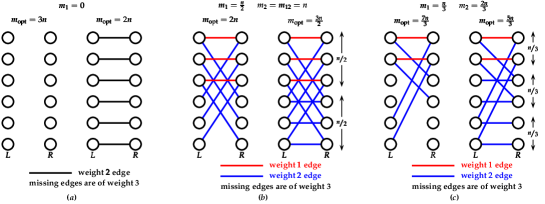
Figure 1: (a) Example showing tightness of bounds in Theorem 5 when only estimate for $m_{1}$ is known. (b) Example showing tightness of bounds in Theorem 5 when estimates for $m_{1},m_{2},m_{12}$ are known; (c) Example showing that better than additive $\frac{2}{3}$-approximation is not possible if only estimates for $m_{1}$ and $m_{2}$ are used for the case in Theorem 5(b).

Proof.

Since $\deg_{G}(u)=\deg_{G}(v)$ we can use the reformulations of the linear program ($\mathsf{LP}$-$\mathfrak{C}_{G}$) outlined in Section 2.2. Let $\delta>0$ be a constant to be fixed later. Let $H_{1}$, $H_{2}$ and $H_{12}$ be the subgraphs of $H$ induced by the edges in $H$ of weight $1$, edges in $H$ of weight $2$, and edges in $H$ of weights $1$ and $2$, respectively. Fix maximum-cardinality matchings $\mathcal{M}_{1}$, $\mathcal{M}_{2}$ and $\mathcal{M}_{12}$ of $H_{1}$, $H_{2}$ and $H_{12}$ having $m_{1}\,n$, $m_{2}\,n$ and $m_{12}\,n$ edges, respectively. Also, fix a minimum-weight perfect matching ${M}_{\mathrm{opt}}$ of $H$ of total weight ${m}_{\mathrm{opt}}\,n$, and let $m_{\mathrm{opt},\ell}\,n$ be the number of edges of weight $\ell\in\{1,2,3\}$ in ${M}_{\mathrm{opt}}$. The following inequalities will be useful during the rest of the proof:

$$m_{\mathrm{opt},1}\leq m_{1},\,\,\,\,m_{\mathrm{opt},2}\leq m_{2},\,\,\,\,m_{\mathrm{opt},3}\geq 1-m_{12},\,\,\,\,m_{12}\geq\max\{m_{1},m_{2}\},$$

$${m}_{\mathrm{opt}}=m_{\mathrm{opt},1}+2\,m_{\mathrm{opt},2}+3(1-m_{\mathrm{opt},1}-m_{\mathrm{opt},2})=3-2\,m_{\mathrm{opt},1}-m_{\mathrm{opt},2}\\ \geq 2-2\,m_{\mathrm{opt},1}\geq 2-2\,m_{1}$$

Let $\mathcal{M}_{s}$ be a perfect matching of $H$ generated by taking all the edges (of weight $1$) in $\mathcal{M}_{1}$ and pairing the remaining nodes from $L$ and $R$ arbitrarily. Note that the total weight $m_{s}\,n$ of the edges in $\mathcal{M}_{s}$ satisfies ${m}_{\mathrm{opt}}\leq m_{s}$ and $m_{s}\leq m_{1}+3(1-m_{1})=3-2\,m_{1}$; thus it follows that $3-2\,m_{1}\geq{m}_{\mathrm{opt}}$. Similarly, taking $\mathcal{M}_{s}$ to be a perfect matching of $H$ of total weight $m_{s}\,n$ generated by taking all the edges (of weight $2$) in $\mathcal{M}_{2}$ and pairing the remaining nodes from $L$ and $R$ arbitrarily we get ${m}_{\mathrm{opt}}\leq m_{s}$ and $m_{s}\leq 2\,m_{2}+3(1-m_{2})=3-m_{2}$; thus it follows that $3-m_{2}\geq{m}_{\mathrm{opt}}$.

Our algorithm proceeds in two main steps. The first common step in our algorithm for both (a) and (b) is to determine the set of nodes in $L$ and $R$ from $\mathsf{Nbr}_{G}(u)$ and $\mathsf{Nbr}_{G}(v)$. This can be done by comparing the list of nodes in $\mathsf{Nbr}_{G}(u)$ and $\mathsf{Nbr}_{G}(v)$ to identify all nodes in $\mathsf{Nbr}_{G}(u)\cap\mathsf{Nbr}_{G}(v)$ and setting $L=\mathsf{Nbr}_{G}(u)\setminus\big{(}\mathsf{Nbr}_{G}(u)\cap\mathsf{Nbr}_{G}(v)\big{)},R=\mathsf{Nbr}_{G}(v)\setminus\big{(}\mathsf{Nbr}_{G}(u)\cap\mathsf{Nbr}_{G}(v)\big{)}$. Note that this step does not use any query at all. The remaining parts of our algorithms will only use weighted neighbor queries $(x,s)$ for $x\in L\cup R$ and $s\in\{1,2\}$.

Proof of (a)

Since $\max_{v\in L\cup R}\{\deg_{H_{1}}(v)\}\leq d$, then using the results of Yoshida et al. [27] we can compute a number $\widetilde{m}_{1}$ using $d^{O(1/\delta^{2})}{(\nicefrac{{1}}{{\delta}})}^{O(1/\delta)}=O(1)$ expected number of queries such that $m_{1}\,n-\delta\,n\leq\widetilde{m}_{1}\,n\leq m_{1}\,n$. It is straightforward to see that each query in Yoshida et al. [27] can be implemented by a weighted neighbor query $(x,1)$ for some appropriate $x\in L\cup R$. After using $O(1)$ expected number of weighted neighbor queries to compute $\widetilde{m}_{1}\,n$ we output the number $\Delta=(3-2\,\widetilde{m}_{1})$ as our estimate for ${m}_{\mathrm{opt}}$. Note that $\Delta\geq(3-2\,{m}_{1})\geq{m}_{\mathrm{opt}}$, and $\Delta-{m}_{\mathrm{opt}}=(3-2\,\widetilde{m}_{1})-{m}_{\mathrm{opt}}\leq(3-2\,{m}_{1})+2\,\delta-{m}_{\mathrm{opt}}\leq 1+2\,\delta$. Our proof is completed by taking $\delta=\nicefrac{{\varepsilon}}{{2}}$.

Proof of (b)

Since $\max_{v\in L\cup R}\{\deg_{H_{1}}(v)\}\leq d$ and $\max_{v\in L\cup R}\{\deg_{H_{2}}(v)\}\leq d$, using the results of Yoshida et al. [27] we can compute numbers $\widetilde{m}_{1}$, $\widetilde{m}_{2}$, and $\widetilde{m}_{12}$ using $(2d)^{O(1/\delta^{2})}{(\nicefrac{{1}}{{\delta}})}^{O(1/\delta)}=O(1)$ expected number of queries such that $m_{\ell}\,n-\delta\,n\leq\widetilde{m}_{\ell}\,n\leq m_{\ell}\,n$ for $\ell\in\{1,2,12\}$. It is straightforward to see that each query in Yoshida et al. [27] can be implemented by a weighted neighbor query $(x,s)$ for some appropriate $x\in L\cup R$ and $s\in\{1,2\}$. We perform the following case analysis to provide our estimate $\Delta$ of ${m}_{\mathrm{opt}}$.

Case 1: $\widetilde{m}_{1}\leq\nicefrac{{1}}{{4}}$.

Our estimate for ${m}_{\mathrm{opt}}$ is $\Delta=3-\widetilde{m}_{2}$. Note that $\Delta\geq 3-m_{2}\geq{m}_{\mathrm{opt}}$. For the additive error estimation, we have

$$\Delta-{m}_{\mathrm{opt}}=3-\widetilde{m}_{2}-{m}_{\mathrm{opt}}\leq(3-{m}_{2}-2m_{1})+2m_{1}+\delta-{m}_{\mathrm{opt}}\\ \leq(3-m_{\mathrm{opt},2}-2\,m_{\mathrm{opt},1})+2\big{(}{\textstyle\frac{1}{4}}+\delta\big{)}+\delta-{m}_{\mathrm{opt}}={\textstyle\frac{1}{2}}+3\,\delta$$

Case 2: $\widetilde{m}_{2}\leq\nicefrac{{1}}{{2}}$ or $\widetilde{m}_{1}\geq\nicefrac{{1}}{{2}}$ or $\widetilde{m}_{12}\leq\nicefrac{{3}}{{4}}$.

Our estimate for ${m}_{\mathrm{opt}}$ is $\Delta=3-2\,\widetilde{m}_{1}$. Note that $\Delta\geq 3-2\,m_{1}\geq{m}_{\mathrm{opt}}$. For the additive error bounds, we have the following:

1. If $\widetilde{m}_{2}\leq\nicefrac{{1}}{{2}}$ then $\Delta-{m}_{\mathrm{opt}}=3-2\,\widetilde{m}_{1}-{m}_{\mathrm{opt}}=(3-m_{2}-2\,m_{1})+m_{2}+2\,\delta-{m}_{\mathrm{opt}}\leq(3-m_{\mathrm{opt},2}-2\,m_{\mathrm{opt},1})+\nicefrac{{1}}{{2}}+3\,\delta-{m}_{\mathrm{opt}}\leq{\textstyle\frac{1}{2}}+3\,\delta$.

2. If $\widetilde{m}_{1}\geq\nicefrac{{1}}{{2}}$ then since the smallest possible total weight that any perfect matching of $H$ could have is achieved by taking all the $m_{1}\,n$ edges of weight $1$ and the remaining $(1-m_{1})\,n$ edges of weight $2$ we get ${m}_{\mathrm{opt}}\geq m_{1}+2(1-m_{1})=2-m_{1}$. Consequently,

   $$\Delta-{m}_{\mathrm{opt}}\leq(3-2\,\widetilde{m}_{1})-(2-m_{1})\leq 1-m_{1}+2\,\delta\leq{\textstyle\frac{1}{2}}+2\,\delta$$

3. If $\widetilde{m}_{12}\leq\nicefrac{{3}}{{4}}$ then since $m_{\mathrm{opt},3}\geq 1-m_{12}$ the smallest possible total weight that any perfect matching of $H$ could achieve is by taking $m_{1}\,n$ edges of weight $1$, $(1-m_{12})n$ edges of weight $3$, and the remaining $(m_{12}-m_{1})n$ edges of weight $2$ we get ${m}_{\mathrm{opt}}\geq m_{1}+2(m_{12}-m_{1})+3(1-m_{12})=3-m_{1}-m_{12}$. Consequently,

   $$\Delta-{m}_{\mathrm{opt}}\leq(3-2\,\widetilde{m}_{1})-(3-m_{1}-m_{12})\leq(m_{12}-m_{1})+2\,\delta\\ \leq({\textstyle\frac{3}{4}}+\delta-{\textstyle\frac{1}{4}})+2\,\delta={\textstyle\frac{1}{2}}+3\,\delta$$

Case 3: when Cases $1$ and Case $2$ do not apply.

For this case the following inequalities hold:

$$<\widetilde{m}_{1}<\nicefrac{{1}}{{2}}\,\Rightarrow\,\nicefrac{{1}}{{4}}<{m}_{1}<\nicefrac{{1}}{{2}}+\delta,\,\,\,\widetilde{m}_{2}>\nicefrac{{1}}{{2}}\,\Rightarrow\,{m}_{2}>\nicefrac{{1}}{{2}}+\delta$$

$$\widetilde{m}_{12}>\nicefrac{{3}}{{4}}\,\Rightarrow\,{m}_{12}>\nicefrac{{3}}{{4}}$$

For this case, we use the following lower bound for ${m}_{\mathrm{opt}}$. Since $m_{\mathrm{opt},3}\geq 1-m_{12}$ the smallest possible total weight that any perfect matching of $H$ could have is achieved by taking $m_{1}\,n$ edges of weight $1$, $(1-m_{12})n$ edges of weight $3$, and the remaining $(m_{12}-m_{1})n$ edges of weight $2$. This implies ${m}_{\mathrm{opt}}\geq m_{1}+2(m_{12}-m_{1})+3(1-m_{12})=3-m_{1}-m_{12}$.

Let $\alpha=\max\{{m}_{12}-2\,{m}_{1},\,0\}$. Suppose that $\mathcal{M}_{12}$ contains $m_{1}^{\prime}\leq m_{1}$ edges of weight $1$. Consider the following process: we start with the edges in $\mathcal{M}_{12}$, remove $m_{1}^{\prime}$ edges of weight $1$ from it, add $m_{1}$ edges of weight $1$ from $\mathcal{M}_{1}$ to it and finally remove (“knock out”) the edges of weight $2$ that share an end-point with the edges of $\mathcal{M}_{1}$ added to our collection. Since $m_{1}$ edges of weight $1$ can knock out at most $2\,m_{1}$ edges of weight $2$, it follows that there are at least $\alpha$ “surviving” edges of weight $2$ that do not share any end-point with the edges in $\mathcal{M}_{1}$. We now have the following two sub-cases.

Case 3.1: $\widetilde{m}_{1,2}\leq 2\,\widetilde{m}_{1}+\delta$.

Note that $\widetilde{m}_{1,2}\leq 2\,\widetilde{m}_{1}+\delta$ implies ${m}_{1,2}\leq 2\,{m}_{1}+2\,\delta$. Our estimate for ${m}_{\mathrm{opt}}$ is $\Delta=3-2\,\widetilde{m}_{1}$. Note that $\Delta\geq 3-2\,m_{1}\geq{m}_{\mathrm{opt}}$. For the additive error estimation, note that

$$\Delta-{m}_{\mathrm{opt}}\leq(3-2\,\widetilde{m}_{1})-(3-m_{1}-m_{12})\leq m_{12}-m_{1}+2\,\delta\\ \leq m_{1}+4\,\delta<{\textstyle\frac{1}{2}}+5\,\delta$$

Case 3.2: $\widetilde{m}_{1,2}>2\,\widetilde{m}_{1}+\delta$.

Our estimate for ${m}_{\mathrm{opt}}$ is $\Delta=3-\widetilde{m}_{1,2}$. Note that $\widetilde{m}_{1,2}>2\,\widetilde{m}_{1}+\delta$ implies ${m}_{1,2}>2\,{m}_{1}+\delta$. Thus, for this case, $\alpha=m_{12}-2\,m_{1}>\delta>0$. Let $\mathcal{M}^{\prime}$ be a perfect matching of $H$ generated by taking all the edges (of weight $1$) in $\mathcal{M}_{1}$, the $\alpha$ surviving edges of weight $2$, and pairing the remaining nodes from $L$ and $R$ arbitrarily. Then, the total weight $m^{\prime}\,n$ of the edges in $\mathcal{M}^{\prime}$ satisfies $m_{1}+2(m_{12}-2\,m_{1})+3(1-(m_{1}+(m_{12}-2\,m_{1})))=3-m_{12}\geq m^{\prime}\geq{m}_{\mathrm{opt}}$, and it follows that $\Delta\geq 3-m_{1,2}\geq{m}_{\mathrm{opt}}$. For the additive error estimation, note that

$$\Delta-{m}_{\mathrm{opt}}\leq(3-\widetilde{m}_{1,2})-(3-m_{1}-m_{12})\leq m_{1}+\delta<{\textstyle\frac{1}{2}}+2\,\delta$$

In all cases, setting $\delta=\nicefrac{{\varepsilon}}{{5}}$ provides an additive $\left(\frac{1}{2}+\varepsilon\right)$-approximation. ∎

5.6 Upper bounds on number of queries for computing $\mathfrak{C}_{G}(e)$ when $\deg(u)\neq\deg(v)$ using “localized” fine-grained reduction

Theorem 5 provides non-trivial approximation of $\mathfrak{C}_{G}(e)$ when $\deg_{G}(u)=\deg_{G}(v)$. In this section, we show that a “localized” version of the fine-grained reduction used in Theorem 3 can be applied to extend these local approximation algorithms to some cases when $\deg_{G}(u)$ and $\deg_{G}(v)$ are not necessarily equal. Such a localized version of the fine-grained reduction is not allowed to construct the reduction explicitly, but instead the details of the reduction need to be revealed incrementally to the local algorithm on a “need-to-know” basis to simulate the queries of the local algorithm on the graph constructed by the fine-grained reduction. The overall simulation is summarized in Theorem 6.

Theorem 6 (Computing $\boldsymbol{\mathfrak{C}_{G}(e)}$ via localized fine-grained reduction).

Suppose that we have an algorithm $\mathfrak{B}_{=}$ that provides an $(\alpha,\varepsilon)$-estimate for $\mathfrak{C}_{G}(e)$ when $\deg_{G}(u)=\deg_{G}(v)$ using $t$ queries $q_{1}^{\prime},\dots,q_{t}^{\prime}$ when each query $q_{i}^{\prime}$ is either a weighted node-pair query, a weighted neighbor query or a weighted selective degree query.

Then, letting $\delta>0$ denote any constant, we can design an algorithm $\mathfrak{B}_{<}$ for the case when $\deg_{G}(u)\neq\deg_{G}(v)$ using $\mathfrak{B}_{=}$ with the following properties:

1. Corresponding to each query $q_{i}^{\prime}$, $\mathfrak{B}_{<}$ performs at most one weighted selective degree query and at most one additional query of the same type as $q_{i}^{\prime}$ on $G_{u,v}$.

2. $\mathfrak{B}_{<}$ provides an $(\alpha,\varepsilon)$-estimate for $\mathfrak{C}_{G}(e)$ if $\deg_{G}(u)+1$ is an integral multiple of $\deg_{G}(v)+1$.

3. $\mathfrak{B}_{<}$ provides an $(\alpha,\varepsilon+\delta)$-estimate for $\mathfrak{C}_{G}(e)$ if either $\deg_{G}(u)\leq(\delta/3)\times\deg_{G}(v)$ or $\deg_{G}(u)\geq(1-(\delta/3)\,)\times\deg_{G}(v)$.

Corollary 7.

If $\deg_{G}(u)\geq(1-(\delta/3)\,)\times\deg_{G}(v)$ for some constant $\delta>0$ then $\max_{x}\{\deg_{G_{u,v},1}(x)\}=O(1)$ $($respectively, $\max_{x}\{\deg_{G_{u,v},2}(x)\}=O(1))$ implies $\max_{x}\{\deg_{G_{u,v}^{\prime},1}(x)\}=O(1)$ $($respectively, $\max_{x}\{\deg_{G_{u,v}^{\prime},2}(x)\}=O(1))$, and thus each weighted selective degree query for the weight $1$ $($respectively, for the weight $2)$ can be trivially simulated by $O(1)$ weighted neighbor queries for the weight $1$ $($respectively, for the weight $2)$ on $G_{u,v}^{\prime}$. Thus, combining Theorem 6 with the approximations in Theorem 5 gives us algorithms of the following types for the case when $\deg_{G}(u)\neq\deg_{G}(v)$:

1. additive $\left(1+\varepsilon+\delta\right)$-approximation using $O(1)$ weighted neighbor queries if $\max_{x}\{\deg_{H,1}(x)\}=O(1)$ and $\deg_{G}(u)\geq(1-(\delta/3)\,)\times\deg_{G}(v)$,

2. additive $\left(\frac{1}{2}+\varepsilon+\delta\right)$-approximation using $O(1)$ weighted neighbor queries if $\max_{x}\{\deg_{H,1}(x)\}=O(1)$, $\max_{x}\{\deg_{H,2}(x)\}=O(1)$, and $\deg_{G}(u)\geq(1-(\delta/3)\,)\times\deg_{G}(v)$.

Proof.

We will reuse the notations and the reduction used in the proof of Theorem 3; in particular in those notations the graph $H$ is also the graph $G_{u,v}$. Our algorithm $\mathfrak{B}_{<}$ has a list of nodes in the graph $G_{u,v}^{\prime}$ and also the numbers $a$ and $b$. We show next how the value of a query $q_{i}^{\prime}$ on $G_{u,v}^{\prime}$ can be obtained from the values of a collection $\mathcal{Q}_{i}$ of (at most two) queries on $G_{u,v}$ by $\mathfrak{B}_{<}$.

1. Case 1: $\boldsymbol{q_{i}^{\prime}}$ is a weighted node-pair query. If $q_{i}^{\prime}$ is of the form $(x_{i}^{j},y_{\ell})$ then $\mathcal{Q}_{i}=\{(x_{i},y_{\ell})\}$ and $\mathfrak{B}_{<}$ returns the value of the query $(x_{i},y_{\ell})$ on $G_{u,v}$ as the value of $q_{i}^{\prime}$. If $q_{i}^{\prime}$ is of the form $(r_{i},y_{\ell})$ then $\mathcal{Q}_{i}=\emptyset$ and $\mathfrak{B}_{<}$ returns $3$ as the value of $q_{i}^{\prime}$.

2. Case 2: $\boldsymbol{q_{i}^{\prime}}$ is a weighted selective degree query. Let $s$ be a number from the set $\{1,2,3\}$.

   • If $q_{i}^{\prime}$ is of the form $(x_{i}^{j},s)$ then $\mathcal{Q}_{i}=\{(x_{i},s)\}$ and $\mathfrak{B}_{<}$ returns the value of the weighted selective degree query $(x_{i},s)$ on $G_{u,v}$ as the value of $q_{i}^{\prime}$.

   • If $q_{i}^{\prime}$ is of the form $(r_{i},s)$ then $\mathcal{Q}_{i}=\emptyset$ and $\mathfrak{B}_{<}$ returns $3\deg_{G}(v)+3$ if $s=3$ and $0$ otherwise as the value of $q_{i}^{\prime}$.

   • If $q_{i}^{\prime}$ is of the form $(y_{\ell},s)$ then $\mathcal{Q}_{i}=\{(y_{\ell},s)\}$, and $\mathfrak{B}_{<}$ returns the following as the value of $q_{i}^{\prime}$:

     • the value of the weighted selective degree query $(y_{\ell},s)$ on $G_{u,v}$ times $a$ if $s\in\{1,2\}$, and

     • the value of the weighted selective degree query $(y_{\ell},s)$ on $G_{u,v}$ times $a$ plus $b$ otherwise.

3. Case 3: $\boldsymbol{q_{i}^{\prime}}$ is a weighted neighbor query. Let $s$ be a number from the set $\{1,2,3\}$.

   1. Case 3.1: $\boldsymbol{q_{i}^{\prime}}$ is of the form $\boldsymbol{(x_{i}^{j},s)}$. The following example illustrates the subtlety of this case. Suppose that $x_{1}$ is connected to four nodes $y_{1},y_{2},y_{3},y_{4}$ via edges of weight $s$ in $G_{u,v}$. Then each of the nodes $x_{1}^{1},\dots,x_{1}^{a}$ is connected to $y_{1},y_{2},y_{3},y_{4}$ via edges of weight $s$ in $G_{u,v}^{\prime}$.

      • As a first attempt, one may simulate the answer to the query $(x_{1}^{j},s)$ by performing a query $(x_{1},s)$ on $G_{u,v}$. However, this will not provide new nodes with the correct probabilities required for random uniform selection among not-yet-explored nodes. For example, suppose that $\mathfrak{B}_{<}$ already made the query $(x_{1}^{1},s)$ giving the node $y_{1}$. If now $\mathfrak{B}_{<}$ makes another query $(x_{1}^{2},s)$ then such a simulation will return a node uniformly randomly from the set of nodes $\{y_{2},y_{3},y_{4}\}$ but the correct simulation would have been to select a node uniformly randomly from the set of nodes $\{y_{1},y_{2},y_{3},y_{4}\}$. Moreover, if $\mathfrak{B}_{<}$ has already made the queries $(x_{1}^{1},s),(x_{1}^{2},s),(x_{1}^{3},s),(x_{1}^{4},s)$ using such a simulation then this simulation of a new query $(x_{1}^{5},s)$ will simply return the special symbol.

      • As a second attempt, to simulate the answer to a query $(x_{1}^{j},s)$ one may first check if the answer to a query $(x_{1}^{j^{\prime}},s)$ for some $j^{\prime}\neq j$ is already available, and if so simply return that answer. But, in this case, the answers to the queries $(x_{1}^{j},s)$ and $(x_{1}^{j^{\prime}},s)$ will not be statistically independent.

      To address these and other subtleties we design Algorithm $\mathfrak{B}_{<}$ to handle all queries of the form $(x_{i}^{j},s)$ for each specific $i$ and $s$ in the following manner. Let $\mathcal{S}_{x_{i},s}$ be the set of (not initially known to $\mathfrak{B}_{<}$) $\sigma_{i,s}=|\mathcal{S}_{x_{i},s}|$ nodes connected to $x_{i}$ in $G_{u,v}$ via edges of weight $s$.

      (i)

      If not already done before, we make one new weighted selective degree query $(x_{i},s)$ on $G_{u,v}$ giving us the value of $\sigma_{i,s}$ (if the value of $\sigma_{i,s}$ is already available we simply use it without making a query).

      (ii)

      For each $x_{i}^{j}$, we keep a count $\kappa_{x_{i}^{j},s}$ of how many times the query $(x_{i}^{j},s)$ has been asked involving the node $x_{i}^{j}$ before the current query and store the answers to these queries in a set $\mathcal{T}_{x_{i}^{j},s}$. We also maintain $\mathcal{T}_{i,s}=\cup_{j=1}^{a}\mathcal{T}_{x_{i}^{j},s}$ and $\kappa_{i,s}=|\mathcal{T}_{i,s}|$. Note the following:

      • If ${\kappa_{x_{i}^{j},s}<\sigma_{i,s}}$ then performing a new weighted neighbor query $\boldsymbol{(x_{i}^{j},s)}$ on $\boldsymbol{G_{u,v}^{\prime}}$ must return a node uniformly at random from the set of nodes ${\Lambda_{x_{i}^{j},s}=\mathcal{S}_{x_{i},s}\setminus\mathcal{T}_{x_{i}^{j},s}}$ with probability ${\nicefrac{{1}}{{\lambda_{x_{i}^{j},s}}}}$ where $\lambda_{x_{i}^{j},s}=|\Lambda_{x_{i}^{j},s}|=\sigma_{i,s}-\kappa_{x_{i}^{j},s}$.

      • If ${\kappa_{i,s}<\sigma_{i,s}}$ then performing a new weighted neighbor query ${(x_{i},s)}$ on $\boldsymbol{G_{u,v}}$ returns a node uniformly at random from the set of nodes ${\Lambda_{i,s}=\mathcal{S}_{x_{i},s}\setminus\mathcal{T}_{i,s}}$ with probability $\nicefrac{{1}}{{\lambda_{i,s}}}$ where $\lambda_{i,s}=|\Lambda_{i,s}|=\sigma_{i,s}-\kappa_{i,s}$.

      • Note that we know all the elements of $\mathcal{T}_{i,s}$; in particular, this means that we can sample a node from a subset of $\boldsymbol{\mathcal{T}_{i,s}}$ uniformly at random.

      (iii)

      For a query $(x_{i}^{j},s)$, we have the following cases.

      1. Case I: $\boldsymbol{\kappa_{i,s}=\sigma_{i,s}}$. In this case $\mathcal{T}_{i,s}=\mathcal{S}_{x_{i},s}$.

         1. Case I-a: $\boldsymbol{\kappa_{x_{i}^{j},s}<\kappa_{i,s}}$. We select a node uniformly at random from the set $\mathcal{T}_{i,s}\setminus\mathcal{T}_{x_{i}^{j},s}=\mathcal{S}_{x_{i},s}\setminus\mathcal{T}_{x_{i}^{j},s}$ and return it as the answer to the query.

         2. Case I-b: $\boldsymbol{\kappa_{x_{i}^{j},s}=\kappa_{i,s}}$. We return an invalid entry as the answer to the query.

      2. Case II: $\boldsymbol{\kappa_{i,s}<\sigma_{i,s}}$. We make a new query $(x_{i},s)$ on $G_{u,v}$ giving us a node $y_{p}\in\Lambda_{i,s}=\mathcal{S}_{x_{i},s}\setminus\mathcal{T}_{i,s}$ with the property that $\Pr[y_{p}\in\Lambda_{i,s}\text{ is returned}\!]=\frac{1}{\lambda_{i,s}}$.

         1. Case II-a: $\boldsymbol{\kappa_{x_{i}^{j},s}=\kappa_{i,s}}$. For this case, $\mathcal{T}_{i,s}=\mathcal{T}_{x_{i}^{j},s}$ and $\lambda_{i,s}=\Lambda_{x_{i}^{j},s}$. We return the node $y_{p}$ as the answer to the query and update all relevant sets and counters appropriately.

         2. Case II-b: $\boldsymbol{\kappa_{x_{i}^{j},s}<\kappa_{i,s}}$. For this case $\mathcal{T}_{x_{i}^{j},s}\subset\mathcal{T}_{i,s}\subset\mathcal{S}_{x_{i},s}$, $\lambda_{i,s}=|\mathcal{S}_{x_{i},s}\setminus\mathcal{T}_{i,s}|>0$, and $\lambda_{x_{i}^{j},s}=|\mathcal{S}_{x_{i},s}\setminus\mathcal{T}_{x_{i}^{j},s}|>\lambda_{i,s}$. We sample the nodes in $\{y_{p}\}\bigcup\big{(}\mathcal{T}_{i,s}\setminus\mathcal{T}_{x_{i}^{j},s}\big{)}$ based on the following probability distribution and update all relevant sets and counters appropriately:

            $$\textstyle\Pr[y_{p}\text{ is selected}\!]=\frac{\lambda_{i,s}}{\lambda_{x_{i}^{j},s}}$$

            $$\textstyle\forall\,y_{\ell}\in\mathcal{T}_{i,s}\setminus\mathcal{T}_{x_{i}^{j},s}\,:\,\Pr[y_{\ell}\text{ is selected}\!]=\frac{1}{\lambda_{x_{i}^{j},s}}$$

            Thus, the answer to the query $(x_{i}^{j},s)$ is selected uniformly at random from the set $\Lambda_{x_{i}^{j},s}=\mathcal{S}_{x_{i},s}\setminus\mathcal{T}_{x_{i}^{j},s}$ since

            $$\begin{array}[]{r l}\textstyle\forall\,y_{\ell}\in\mathcal{S}_{x_{i},s}\setminus\mathcal{T}_{i,s}\,:&\textstyle\Pr[y_{\ell}\text{ is selected}\!]=\frac{1}{\lambda_{i,s}}\times\frac{\lambda_{i,s}}{\lambda_{x_{i}^{j},s}}==\frac{1}{\lambda_{x_{i}^{j},s}}\\ \textstyle\forall\,y_{\ell}\in\mathcal{T}_{i,s}\setminus\mathcal{T}_{x_{i}^{j},s}\,:&\textstyle\Pr[y_{\ell}\text{ is selected}\!]=\frac{1}{\lambda_{x_{i}^{j},s}}\end{array}$$

   2. Case 3.2: $\boldsymbol{q_{i}^{\prime}}$ is of the form $\boldsymbol{(r_{i},s)}$. We keep a count $\nu(r_{i})$ of how many times the query $(r_{i},3)$ has been asked involving the node $r_{i}$ before the current query, and store the answers to these queries in the set $\mathcal{S}_{r_{i}}$. If $s\neq 3$ or $\nu(r_{i})=\deg_{G}(v)+1$ we return the special symbol. Otherwise, we return a node selected uniformly at random from the set of nodes $\{y_{1},\dots,y_{\deg_{G}(v)+1}\}\setminus\mathcal{S}_{r_{i}}$ as the answer and update all relevant sets and counters appropriately.

   3. Case 3.3: $\boldsymbol{q_{i}^{\prime}}$ is of the form $\boldsymbol{(y_{\ell},s)}$. This case is similar in spirit to Case 3.1. We show how to handle all queries of the form $(y_{\ell},s)$ for each specific $\ell$ and $s$.

      (i)

      Assume without loss of generality that $y_{\ell}$ is connected, via edges of weight $s$, to (not initially known to $\mathfrak{B}_{<}$) a set $\mathcal{S}_{\nu_{1}}=\{x_{1},\dots,x_{\nu_{1}}\}\subseteq\{x_{1},\dots,x_{\deg_{G}(u)+1}\}$ of $\nu_{1}=|\mathcal{S}_{\nu_{1}}|$ nodes. If not already done before, we make one new weighted selective degree query $(y_{\ell},s)$ on $G_{u,v}$ giving us the value of $\nu_{1}$ (if $\nu_{1}$ is already known we simply use it without making a query).

      (ii)

      Define the set $\mathcal{S}_{\nu_{2}}$ of $\nu_{2}=|\mathcal{S}_{\nu_{2}}|\in\{0,b\}$ nodes as $\mathcal{S}_{\nu_{2}}=\{r_{1},\dots,r_{b}\}$ if $s=3$ and $\mathcal{S}_{\nu_{2}}=\emptyset$ otherwise. Note that we know the value of $\nu_{2}$ since we know the value of $s$.

      (iii)

      We keep a count $\kappa$ of how many times the query $(y_{\ell},s)$ has been asked involving the node $y_{\ell}$ before the current query, and let $\mathcal{T}_{\kappa}$ be the set of those $\kappa=|\mathcal{T}_{\kappa}|$ nodes of $\boldsymbol{G_{u,v}^{\prime}}$ that have been returned because of these prior queries. Note that if $\boldsymbol{\kappa<a\,\nu_{1}+\nu_{2}}$ then performing a new weighted neighbor query $\boldsymbol{(y_{\ell},s)}$ on $\boldsymbol{G_{u,v}^{\prime}}$ must return a node uniformly at random from the set of nodes $\boldsymbol{\Lambda_{\kappa}=\big{(}\cup_{i=1}^{\nu_{1}}\cup_{j=1}^{a}\{x_{i}^{j}\}\cup\mathcal{S}_{\nu_{2}}\big{)}\setminus\mathcal{T}_{\kappa}}$ with probability $\boldsymbol{\nicefrac{{1}}{{\lambda_{\kappa}}}}$ where $\boldsymbol{\lambda_{\kappa}=|\Lambda_{\kappa}|=(a\,\nu_{1}+\nu_{2})-\kappa}$.

      (iv)

      Assume without loss of generality that $\mathcal{S}_{\nu_{1}}^{\prime}=\{x_{1},x_{2},\dots,x_{\nu_{1}^{\prime}}\}\subseteq\mathcal{S}_{\nu_{1}}$ be the set of $\nu_{1}^{\prime}=|\mathcal{S}_{\nu_{1}}^{\prime}|\leq\min\{\kappa,\nu_{1}\}\}$ nodes in $\boldsymbol{G_{u,v}}$ that have been returned as a result of the queries on $G_{u,v}$ due to the simulation of prior $\kappa$ queries on $G_{u,v}^{\prime}$. Note that if $\boldsymbol{\nu_{1}^{\prime}<\nu_{1}}$ then performing a new weighted neighbor query $\boldsymbol{(y_{\ell},s)}$ on $\boldsymbol{G_{u,v}}$ returns a new node uniformly at random from the set of nodes $\boldsymbol{\Phi=\mathcal{S}_{\nu_{1}}\setminus\mathcal{S}_{\nu_{1}}^{\prime}}$ with probability $\boldsymbol{\nicefrac{{1}}{{\varphi}}}$ where $\boldsymbol{\varphi=|\Phi|=\nu_{1}-\nu_{1}^{\prime}}$.

      (v)

      Define the subset $\Lambda_{\kappa}^{\prime}\subseteq\Lambda_{\kappa}$ of nodes of $G_{u,v}^{\prime}$ as $\Lambda_{\kappa}^{\prime}=\big{(}\cup_{i=1}^{\nu_{1}^{\prime}}\cup_{j=1}^{a}\{x_{i}^{j}\}\cup\mathcal{S}_{\nu_{2}}\big{)}\setminus\mathcal{T}_{\kappa}$. Note that we know all the elements of $\Lambda_{\kappa}^{\prime}$ and $\lambda_{\kappa}^{\prime}=|\Lambda_{\kappa}^{\prime}|=(a\nu_{1}^{\prime}+\nu_{2})-\kappa$. In particular, this means that we can sample a node from $\boldsymbol{\Lambda_{\kappa}^{\prime}}$ uniformly at random.

      (vi)

      For a new query $(y_{\ell},s)$, we have the following cases.

      1. Case I: $\boldsymbol{\kappa\geq\nu_{1}}$. In this case, $\nu_{1}^{\prime}=\nu_{1}$, $\Lambda_{\kappa}^{\prime}=\Lambda_{\kappa}$ and $\lambda_{\kappa}^{\prime}=\lambda_{\kappa}$. We select as our answer to the query a node uniformly at random from $\Lambda_{\kappa}^{\prime}$, and update all relevant sets and counters appropriately.

      2. Case II: $\boldsymbol{\kappa<\nu_{1}}$. In this case, $\nu_{1}^{\prime}<\nu_{1}$, and $\varphi>0$. We simulate the query as follows.

         • We make a new query $(y_{\ell},s)$ on $G_{u,v}$ giving us a node $x_{p}\in\Phi$ for $p\in\{\nu_{1}^{\prime}+1,\dots,\nu_{1}\}$ with probability $\nicefrac{{1}}{{\varphi}}$. We select $j\in\{1,\dots,a\}$ uniformly at random giving us a node $x_{p}^{j}$.

         • We sample a node from $\{x_{p}^{j}\}\cup\Lambda_{\kappa}^{\prime}$ based on the following probability distribution and update all relevant sets and counters appropriately:

           $$\textstyle\Pr[x_{p}^{j}\text{ is selected }\!]=\frac{a\varphi}{\lambda_{\kappa}}$$

           $$\textstyle\forall\,x_{i}^{j}\in\Lambda_{\kappa}^{\prime}\,:\,\Pr[x_{i}^{j}\text{ is selected }\!]=\frac{1}{\lambda_{\kappa}}$$

           Note that $\Pr[x_{i}^{j}\in\Lambda_{\kappa}\setminus\Lambda_{\kappa}^{\prime}\text{ is selected }\!]=\frac{1}{a\varphi}\times\frac{a\varphi}{\lambda_{\kappa}}=\frac{1}{\lambda_{\kappa}}$, as desired. To verify that all the probabilities add up to $1$, note that $\Pr[x_{p}^{j}\text{ is selected }\!]+\sum_{x_{i}^{j}\in\Lambda_{\kappa}^{\prime}}\Pr[x_{i}^{j}\in\Lambda_{\kappa}^{\prime}\text{ is selected }\!]=\frac{a(\nu_{1}-\nu_{1}^{\prime})}{a\nu_{1}+\nu_{2}-\kappa}+(a\nu_{1}^{\prime}+\nu_{2}-\kappa)\times\frac{1}{a\nu_{1}+\nu_{2}-\kappa}=1$.

∎

6 Computing $\mathfrak{C}_{G}(v)$ and $\mathfrak{C}_{\mathrm{avg}}(G)$ using “black box” additive approximation algorithms for $\mathfrak{C}_{G}(e)$

In this section we provide efficient local algorithms to compute $\mathfrak{C}_{G}(v)$ and $\mathfrak{C}_{\mathrm{avg}}(G)$. The following assumptions are used by our algorithms:

1. For a fixed $\mathfrak{r}$, we have an efficient local algorithm $\mathfrak{B}$ for an additive $\mathfrak{r}$-approximation, say $\mathfrak{C}_{G}^{\,\mathfrak{r}}(e)$, of $\mathfrak{C}_{G}(e)$ for an edge $e$.

2. We have access to the neighbor query model mentioned in Section 5.2.

Lemma 8.

With probability at least $\nicefrac{{2}}{{3}}$ the following two claims hold.

1. We can compute an additive $2\mathfrak{r}$-approximation of $\mathfrak{C}_{G}(v)$ using $O(1/\mathfrak{r}^{2})$ neighbor queries and $O(1/\mathfrak{r}^{2})$ invocations of algorithm $\mathfrak{B}$ on the edges incident on $v$, and

2. If the degrees of all the nodes of $G$ are know then we can compute an additive $2\mathfrak{r}$-approximation of $\mathfrak{C}_{\mathrm{avg}}(G)$ using $O(1/\mathfrak{r}^{2})$ neighbor queries and $O(1/\mathfrak{r}^{2})$ invocations of algorithm $\mathfrak{B}$ over all edges in $G$.

Proof.

(a) Let $k$ be a parameter to be specified later. We use $k^{\prime}=\min\{k,\deg_{G}(v)\}$ neighbor queries to get $k^{\prime}$ nodes adjacent to $v$, say $u_{1},\dots,u_{k^{\prime}}$, compute $\mathfrak{C}_{G}^{\,\mathfrak{r}}(v,u_{1}),\dots,\mathfrak{C}_{G}^{\,\mathfrak{r}}(v,u_{k^{\prime}})$ using algorithm $\mathfrak{B}$, and return $\widetilde{\mathfrak{C}_{G}}(v)=\frac{1}{k^{\prime}}\sum_{j=1}^{k^{\prime}}\mathfrak{C}_{G}^{\,\mathfrak{r}}(v,u_{j})$ as our answer.

If $k>\deg_{G}(v)$ then $\mathfrak{C}_{G}(v)=\frac{1}{k^{\prime}}\sum_{j=1}^{k^{\prime}}\mathfrak{C}_{G}(v,u_{j})$ and thus $\widetilde{\mathfrak{C}_{G}}(v)$ is in fact an additive $\mathfrak{r}$-approximation of $\mathfrak{C}_{G}(v)$. Otherwise, assume that $k\leq\deg_{G}(v)$ and therefore $k^{\prime}=k$. For any number $x$, we use the notation $x\boxplus\rho$ to indicate a number $y$ that satisfies $x\leq y\leq x+\rho$. Observe that

$$\mathbb{E}\left[\widetilde{\mathfrak{C}_{G}}(v)\right]=\frac{1}{k}\sum_{j=1}^{k}\mathbb{E}\left[\mathfrak{C}_{G}^{\,\mathfrak{r}}(v,u_{j})\right]=\frac{1}{k}\sum_{j=1}^{k}\sum_{u\in\mathsf{Nbr}_{G}(u)}(\mathfrak{C}_{G}((u,v))\boxplus\mathfrak{r})\times\frac{1}{\deg_{G}(v)}\\ =\frac{1}{k}\sum_{j=1}^{k}(\mathfrak{C}_{G}(v)\boxplus\mathfrak{r})=\mathfrak{C}_{G}(v)\boxplus\mathfrak{r}$$

Since the $\frac{1}{k}\mathfrak{C}_{G}^{\,\mathfrak{r}}(v,u_{j})$’s are mutually independent for $j=1,\dots,k$, and each $\frac{1}{k}\mathfrak{C}_{G}^{\,\mathfrak{r}}(v,u_{j})$ lies in the interval $[-2/k,1/k]$ (cf. see Section 2.3), applying Hoeffding’s inequality [43, Theorem 2] we get

$$\Pr[\widetilde{\mathfrak{C}_{G}}(v)>\mathfrak{C}_{G}(v)+2\mathfrak{r}]\leq\Pr[\widetilde{\mathfrak{C}_{G}}(v)>{\mathbb{E}}[\widetilde{\mathfrak{C}_{G}}(v)]+\mathfrak{r}]$$

$$\textstyle<\exp\left(-\frac{2\mathfrak{r}^{2}}{\sum^{k}_{i=1}(2/k-(-1/k))^{2}}\right)=\exp\left(-\frac{2}{9}k^{2}\mathfrak{r}^{2}\right)$$

Setting $k=\Theta(\mathfrak{r}^{-2})$ we get $\Pr[\widetilde{\mathfrak{C}_{G}}(v)>\mathfrak{C}_{G}(v)+2\mathfrak{r}]<\nicefrac{{1}}{{3}}$.

(b) The algorithm and its proof is very similar to those in (a). For this case, we need to randomly sample $k^{\prime}=\min\{O(1/\mathfrak{r}^{2}),,|E|\}$ edges $e_{1},\dots,e_{k^{\prime}}$ from $E$, compute $\mathfrak{C}_{G}^{\,\mathfrak{r}}(e_{1}),\dots,\mathfrak{C}_{G}^{\,\mathfrak{r}}(e_{k^{\prime}})$ using algorithm $\mathfrak{B}$, and return $\frac{1}{k^{\prime}}\sum_{j=1}^{k^{\prime}}\mathfrak{C}_{G}^{\,\mathfrak{r}}(e_{j})$ as our answer. The only remaining part of the proof is to show how to sample an edge uniformly at random from the set of edges $E$ of $G$. Since the degrees of all nodes are known, the following procedure can be used. We first select a node $x\in V$ with probability $\frac{\deg_{G}(x)}{\sum_{z\in V}\deg_{G}(z)}$, then we select a random neighbor of $x$, say $y$, using one neighbor query, and finally we select the edge $\{x,y\}$. The proof is completed by observing that

$$\textstyle\Pr[\{u,v\}\in E\text{ is selected}]\\ \textstyle=\Pr[x\in V\text{ is selected}]\times\Pr[y\in\mathsf{Nbr}_{G}(x)\text{ is selected}]\\ \textstyle\hskip 21.68121pt+\Pr[y\in V\text{ is selected}]\times\Pr[x\in\mathsf{Nbr}_{G}(y)\text{ is selected}]\\ \textstyle=\frac{\deg_{G}(x)}{\sum_{z\in V}\deg_{G}(z)}\times\frac{1}{\deg_{G}(x)}+\frac{\deg_{G}(y)}{\sum_{z\in V}\deg_{G}(z)}\times\frac{1}{\deg_{G}(y)}=\frac{1}{|E|}$$

∎

7 Concluding remarks

We hope that this paper will stimulate further attention from computer scientists concerning the exciting interplay between notions of curvatures from network and non-network domains. An obvious candidate for future research is improvement of the query complexities for local algorithms for computing the Ollivier-Ricci curvature for networks. Another possible future research direction is to investigate computational complexity issues of other discretizations of Ricci curvatures. For example, another discretization of Ricci curvature for networks proposed by Ollivier and Villani [44] is guided by the observation that the infinite-dimensional version of the well-known Brunn-Minkowski inequality over ${\mathbb{R}}^{n}$ [45] can be tightened in the presence of a positive curvature for a smooth Riemannian manifold [46, 47]. To our knowledge, these discretizations have largely escaped computational complexity considerations.

Appendix A A self-contained proof of Fact 1

Let $\deg_{G}(u)=\deg_{G}(v)=\alpha$. Build a directed single-source single-sink flow network [48] $G_{u,v}^{f}$ from $G_{u,v}$ in the following manner: add a new source node $s$ and a new sink node $t$, add an arc (directed edge) from $s$ to every node of $L_{u,v}^{G}$ of weight zero and capacity $1$, add an arc from every node of $R_{u,v}^{G}$ to $t$ of weight zero and capacity $1$, orient every edge $\{{u^{\prime}},{v^{\prime}}\}$ of $G_{u,v}$ from ${u^{\prime}}$ to ${v^{\prime}}$ and set its capacity to $1$. Since $|L_{u,v}^{G}|=|R_{u,v}^{G}|=\alpha+1$, we have ${\mathbb{P}}_{u}^{G}(u^{\prime})={\mathbb{P}}_{v}^{G}(v^{\prime})=\frac{1}{\alpha+1}$ for all $u^{\prime}\in\mathsf{Nbr}^{G}(u)\cup\{u\}$ and $v^{\prime}\in\mathsf{Nbr}^{G}(v)\cup\{v\}$. Thus, since $G_{u,v}$ is a complete bipartite graph, by a simple scaling it follows that $\text{{\sc Emd}}_{\!\!\!G_{u,v}}({\mathbb{P}}_{u}^{G},{\mathbb{P}}_{v}^{G})=\frac{\mathcal{M}}{\alpha+1}$ where $\mathcal{M}$ is the total weight of a minimum-weight maximum $s$-$t$ flow on $G_{u,v}^{f}$. Since the node-arc incidence matrix of a directed graph is totally unimodular, the flow value of every arc of any extreme-point optimal solution of the minimum-weight maximum $s$-$t$ flow on $G_{u,v}^{f}$ is integral and therefore $0$ or $1$ (see Theorem $13.3$ and its corollary in [48]). This integrality of flow values and the fact that $G_{u,v}$ is a complete bipartite graph imply $\mathcal{M}$ is also the total weight of a minimum-weight perfect matching of $G_{u,v}$.

We now show that there is such a minimum-weight perfect matching that uses all the zero-weight edges $\{{u^{\prime}},{u^{\prime}}\}$ for all $u^{\prime}\in\{u,v\}\cup\big{(}\,\mathsf{Nbr}_{G}(u)\cap\mathsf{Nbr}_{G}(v)\,\big{)}$. For a contradiction, suppose that the edge $\{{u^{\prime}},{u^{\prime}}\}$ is not used for some $u^{\prime}\in\{u,v\}\cup(\mathsf{Nbr}_{G}(u)\cap\mathsf{Nbr}_{G}(v))\}$. Since our solution is a perfect matching, the nodes ${u^{\prime}}\in L_{u,v}^{G}$ and ${u^{\prime}}\in R_{u,v}^{G}$ must be matched to some other nodes, say to nodes ${v^{\prime\prime}}\in R_{u,v}^{G}$ and $u^{\prime\prime}\in L_{u,v}^{G}$, respectively. Then, if we instead use the edges $\{{u^{\prime}},{u^{\prime}}\}$ and $\{{u^{\prime\prime}},{v^{\prime\prime}}\}$ then using the triangle inequality it follows that the total weight of this modified perfect matching is no more than that of the original perfect matching since:

$$w_{u,v}^{G}({u^{\prime}},{u^{\prime}})+w_{u,v}^{G}({u^{\prime\prime}},{v^{\prime\prime}})=w_{u,v}^{G}({u^{\prime\prime}},{v^{\prime\prime}})\leq w_{u,v}^{G}({u^{\prime\prime}},{u^{\prime}})+w_{u,v}^{G}({u^{\prime}},{u^{\prime}})+w_{u,v}^{G}({u^{\prime}},{v^{\prime\prime}})\\ =w_{u,v}^{G}({u^{\prime\prime}},{u^{\prime}})+w_{u,v}^{G}({u^{\prime}},{v^{\prime\prime}})$$

References

- [1] M. R. Bridson, A. Häfliger, Metric Spaces of Non-Positive Curvature, 1st Edition, Springer-Verlag Berlin Heidelberg, 1999. doi:10.1007/978-3-662-12494-9.
- [2] M. Berger, A Panoramic View of Riemannian Geometry, 1st Edition, Springer-Verlag Berlin Heidelberg, 2003. doi:10.1007/978-3-642-18245-7.
-
[3]
R. Albert, B. DasGupta, N. Mobasheri,
Topological
implications of negative curvature for biological and social networks,
Physical Review E 89 (2014) 032811.
doi:10.1103/PhysRevE.89.032811.
URL https://link.aps.org/doi/10.1103/PhysRevE.89.032811 - [4] T. Chatterjee, R. Albert, S. Thapliyal, N. Azarhooshang, B. DasGupta, Detecting network anomalies using forman-ricci curvature and a case study for human brain networks, Scientific Reports 11 (2021). doi:10.1038/s41598-021-87587-z.
-
[5]
E. Jonckheere, M. Lou, F. Bonahon, Y. Baryshnikov,
Euclidean versus
hyperbolic congestion in idealized versus experimental networks, Internet
Mathematics 71 (2011) 1–27.
doi:10.1080/15427951.2010.554320.
URL https://doi.org/10.1080/15427951.2010.554320 - [6] J. Sia, E. Jonckheere, P. Bogdan, Ollivier-ricci curvature-based method to community detection in complex networks, Scientific Reports 9 (2019) 9800. doi:10.1038/s41598-019-46079-x.
- [7] A. K. Simhal, K. L. H. Carpenter, S. Nadeem, J. Kurtzberg, A. Song, A. Tannenbaum, G. Sapiro, G. Dawson, Measuring robustness of brain networks in autism spectrum disorder with Ricci curvature, Scientific Reports 10 (2020) 10819. doi:10.1038/s41598-020-67474-9.
-
[8]
P. Elumalai, Y. Yadav, N. Williams, E. Saucan, J. Jost, A. Samal,
Graph
ricci curvatures reveal atypical functional connectivity in autism spectrum
disorder, bioRxiv (2021).
doi:10.1101/2021.11.28.470231.
URL https://www.biorxiv.org/content/early/2021/12/21/2021.11.28.470231 - [9] B. Chow, F. Luo, Combinatorial ricci flows on surfaces, Journal of Differential Geometry 63 (1) (2003) 97–129. doi:10.4310/jdg/1080835659.
-
[10]
Y. Ollivier, A visual
introduction to Riemannian curvatures and some discrete
generalizations, in: G. Dafni, R. J. McCann, A. Stancu (Eds.), Analysis and
Geometry of Metric Measure Spaces: Lecture Notes of the 50th Séminaire de
Mathématiques Supérieures (SMS), Montréal, 2011, Vol. 56,
American Mathematical Society, Providence, RI, USA, 2013, pp. 197–219.
doi:10.1090/crmp/056/08.
URL https://hal.archives-ouvertes.fr/hal-00858008 - [11] Y. Ollivier, Ricci curvature of markov chains on metric spaces, Journal of Functional Analysis 256 (2009) 810–864. doi:10.1016/j.jfa.2008.11.001.
- [12] Y. Ollivier, A survey of ricci curvature for metric spaces and markov chains, in: M. Kotani, M. Hino, T. Kumagai (Eds.), Advanced Studies in Pure Mathematics, Vol. 57, Mathematical Society of Japan, 2010, pp. 343–381. doi:10.2969/aspm/05710343.
-
[13]
Y. Ollivier,
Ricci
curvature of metric spaces, Comptes Rendus Mathematique 345 (11) (2007)
643–646.
doi:10.1016/j.crma.2007.10.041.
URL https://www.sciencedirect.com/science/article/pii/S1631073X07004414 - [14] B. DasGupta, M. V. Janardhanan, F. Yahyanejad, Why did the shape of your network change? (on detecting network anomalies via non-local curvatures), Algorithmica 82 (7) (2020) 1741–1783. doi:10.1007/s00453-019-00665-7.
- [15] B. DasGupta, M. Karpinski, N. Mobasheri, F. Yahyanejad, Effect of gromov-hyperbolicity parameter on cuts and expansions in graphs and some algorithmic implications, Algorithmica 80 (2) (2018) 772–800. doi:10.1007/s00453-017-0291-7.
- [16] I. Benjamini, Expanders are not hyperbolic, Israel Journal of Mathematics 108 (1998) 33–36. doi:10.1007/BF02783040.
- [17] J. Chalopin, V. Chepoi, F. F. Dragan, G. Ducoffe, A. M. A., Y. Vaxès, Fast approximation and exact computation of negative curvature parameters of graphs., Discrete and Computational Geometry 65 (2021) 856–892. doi:10.1007/s00454-019-00107-9.
-
[18]
H. Fournier, A. Ismail, A. Vigneron,
Computing the gromov
hyperbolicity of a discrete metric space, Information Processing Letters
115 (6) (2015) 576–579.
doi:10.1016/j.ipl.2015.02.002.
URL https://doi.org/10.1016/j.ipl.2015.02.002 - [19] R. Forman, Bochner’s method for cell complexes and combinatorial ricci curvature, Discrete and Computational Geometry 29 (3) (2003) 323–374. doi:10.1007/s00454-002-0743-x.
- [20] R. P. Sreejith, K. Mohanraj, J. Jost, E. Saucan, A. Samal, Forman curvature for complex networks, Journal of Statistical Mechanics: Theory and Experiment 2016 (6) (2016) 063206. doi:10.1088/1742-5468/2016/06/063206.
-
[21]
R. P. Sreejith, J. Jost, E. Saucan, A. Samal,
Systematic
evaluation of a new combinatorial curvature for complex networks, Chaos,
Solitons and Fractals 101 (2017) 50–67.
doi:10.1016/j.chaos.2017.05.021.
URL https://www.sciencedirect.com/science/article/pii/S0960077917302102 - [22] M. Weber, E. Saucan, J. Jost, Characterizing complex networks with forman-ricci curvature and associated geometric flows, Journal of Complex Networks 5 (4) (2017) 527–550. doi:10.1093/comnet/cnw030.
- [23] A. Samal, R. P. Sreejith, J. Gu, S. Liu, E. Saucan, J. Jost, Comparative analysis of two discretizations of ricci curvature for complex networks, Scientific Reports 8 (2018) 8650. doi:10.1038/s41598-018-27001-3.
- [24] M. Gromov, Hyperbolic groups, in: S. M. Gersten (Ed.), Essays in Group Theory, Vol. 8, Springer, New York, NY, 1987, pp. 75–263. doi:10.1007/978-1-4613-9586-7\_3.
-
[25]
V. Chepoi, F. Dragan, B. Estellon, M. Habib, Y. Vaxès,
Diameters, centers, and
approximating trees of delta-hyperbolicgeodesic spaces and graphs, in:
Proceedings of the Twenty-Fourth Annual Symposium on Computational Geometry,
SCG ’08, Association for Computing Machinery, New York, NY, USA, 2008, pp.
59–68.
doi:10.1145/1377676.1377687.
URL https://doi.org/10.1145/1377676.1377687 - [26] F. Papadopoulos, D. Krioukov, M. Boguna, A. Vahdat, Greedy forwarding in dynamic scale-free networks embedded in hyperbolic metric spaces, in: 2010 Proceedings IEEE INFOCOM, 2010, pp. 1–9. doi:10.1109/INFCOM.2010.5462131.
- [27] Y. Yoshida, M. Yamamoto, H. Ito, Improved Constant-Time Approximation Algorithms for Maximum Matchings and Other Optimization Problems, SIAM Journal on Computing 41 (4) (2012) 1074–1093. doi:10.1137/110828691.
- [28] Y. T. Lee, A. Sidford, Efficient inverse maintenance and faster algorithms for linear programming, in: 2015 IEEE 56th Annual Symposium on Foundations of Computer Science, 2015, pp. 230–249. doi:10.1109/FOCS.2015.23.
-
[29]
K. Quanrud,
Approximating
Optimal Transport With Linear Programs, in: J. T. Fineman, M. Mitzenmacher
(Eds.), 2nd Symposium on Simplicity in Algorithms (SOSA 2019), Vol. 69 of
OpenAccess Series in Informatics (OASIcs), Schloss Dagstuhl–Leibniz-Zentrum
fuer Informatik, Dagstuhl, Germany, 2018, pp. 6:1—6:9.
doi:10.4230/OASIcs.SOSA.2019.6.
URL http://drops.dagstuhl.de/opus/volltexte/2018/10032 -
[30]
P. Dvurechensky, A. Gasnikov, A. Kroshnin,
Computational
optimal transport: Complexity by accelerated gradient descent is better than
by sinkhorn’s algorithm, in: J. Dy, A. Kraus (Eds.), Proceedings of the 35th
International Conference on Machine Learning, Vol. 80 of Proceedings of
Machine Learning Research, PMLR, 2018, pp. 1367—1376.
URL https://proceedings.mlr.press/v80/dvurechensky18a.html - [31] N. Azarhooshang, P. Sengupta, B. DasGupta, A review of and some results for ollivier-ricci network curvature, Mathematics 8 (1416) (2020). doi:10.3390/math8091416.
-
[32]
G. Peyré, M. Cuturi,
Computational optimal transport:
With applications to data science, Foundations and Trends in Machine
Learning 11 (5–6) (2019) 355–607.
doi:10.1561/2200000073.
URL http://dx.doi.org/10.1561/2200000073 -
[33]
A. L. Gibbs, F. E. Su, On choosing
and bounding probability metrics, International Statistical Review / Revue
Internationale de Statistique 70 (3) (2002) 419–435.
doi:10.2307/1403865.
URL http://www.jstor.org/stable/1403865 - [34] V. V. Williams, On some fine-grained questions in algorithms and complexity, in: Proceedings of the International Congress of Mathematicians (ICM 2018), 2019, pp. 3447–3487. doi:10.1142/9789813272880\_0188.
- [35] A. Abboud, F. Grandoni, V. V. Williams, Subcubic equivalences between graph centrality problems, apsp and diameter, in: Proceedings of the Twenty-Sixth Annual ACM-SIAM Symposium on Discrete Algorithms, SODA ’15, Society for Industrial and Applied Mathematics, USA, 2015, pp. 1681–1697.
-
[36]
M. Patrascu, Towards polynomial
lower bounds for dynamic problems, in: Proceedings of the Forty-Second ACM
Symposium on Theory of Computing, STOC ’10, Association for Computing
Machinery, New York, NY, USA, 2010, pp. 603–610.
doi:10.1145/1806689.1806772.
URL https://doi.org/10.1145/1806689.1806772 -
[37]
L. Lee, Fast context-free grammar
parsing requires fast boolean matrix multiplication, Journal of the ACM
49 (1) (2002) 1–15.
doi:10.1145/505241.505242.
URL https://doi.org/10.1145/505241.505242 -
[38]
M. Parnas, D. Ron,
Approximating
the minimum vertex cover in sublinear time and a connection to distributed
algorithms, Theoretical Computer Science 381 (1) (2007) 183–196.
doi:https://doi.org/10.1016/j.tcs.2007.04.040.
URL https://www.sciencedirect.com/science/article/pii/S0304397507003696 - [39] K. Onak, D. Ron, M. Rosen, R. Rubinfeld, A near-optimal sublinear-time algorithm for approximating the minimum vertex cover size, in: Proceedings of the twenty-third annual ACM-SIAM symposium on Discrete Algorithms, SIAM, 2012, pp. 1123–1131.
- [40] K. D. Ba, H. L. Nguyen, H. N. Nguyen, R. Rubinfeld, Sublinear time algorithms for earth mover’s distance, Theory of Computing Systems 48 (2) (2011) 428–442. doi:10.1007/s00224-010-9265-8.
- [41] A. McGregor, D. Stubbs, Sketching earth-mover distance on graph metrics, in: P. Raghavendra, S. Raskhodnikova, K. Jansen, J. D. P. Rolim (Eds.), Approximation, Randomization, and Combinatorial Optimization. Algorithms and Techniques, Lecture Notes in Computer Science, Vol. 8096, Springer, Berlin, Heidelberg, 2013, pp. 274–286. doi:10.1007/978-3-642-40328-6\_20.
- [42] A. C.-C. Yao, Probabilistic computations: Toward a unified measure of complexity, in: 18th Annual Symposium on Foundations of Computer Science, 1977, pp. 222–227. doi:10.1109/SFCS.1977.24.
-
[43]
W. Hoeffding, Probability
inequalities for sums of bounded random variables, Journal of the American
Statistical Association 58 (301) (1963) 13–30.
URL http://www.jstor.org/stable/2282952 -
[44]
Y. Ollivier, C. Villani, A curved
brunn–minkowski inequality on the discrete hypercube, or: What is the ricci
curvature of the discrete hypercube?, SIAM Journal on Discrete Mathematics
26 (3) (2012) 983–996.
arXiv:https://doi.org/10.1137/11085966X, doi:10.1137/11085966X.
URL https://doi.org/10.1137/11085966X - [45] R. J. Gardner, The Brunn-Minkowski inequality, Bulletin of American Mathematical Society 39 (3) (2002) 355–405. doi:10.1090/S0273-0979-02-00941-2.
- [46] D. Cordero-Erausquin, R. J. McCann, M. Schmuckenschläger, A riemannian interpolation inequality à la borell, brascamp and lieb, Inventiones Mathematicae 146 (2001) 219–257. doi:10.1007/s002220100160.
-
[47]
D. Cordero-Erausquin, R. J. McCann, M. Schmuckenschläger,
Prékopa–leindler
type inequalities on Riemannian manifolds, Jacobi fields, and optimal
transport, Annales de la Faculté des sciences de Toulouse :
Mathématiques Ser. 6, 15 (4) (2006) 613–635.
doi:10.5802/afst.1132.
URL https://afst.centre-mersenne.org/articles/10.5802/afst.1132/ - [48] C. H. Papadimitriou, K. Steiglitz, Combinatorial optimization: algorithms and complexity, Prentice-Hall, Inc., NJ, USA, 1982.